do regional climate models reproduces the spatial ... · driving gcm institute model acronym...
TRANSCRIPT
Do regional climate models reproducesthe spatial distribution of monthlyprecipitation in the Mediterraneanregion better than global models?
P. Lionello, L.CongediUniversity of Salento, <[email protected]>

Aim:To analyze the monthly precipitation (and temperature) fields of Regionalclimate models (RCMs) that cover the whole Mediterranean region in the ENSEMBLES and PRUDENCE projects and compare them with the global climate models (GCMs) providing the initial and boundary conditions.
Motivation:RCMs are expected to produce more accurate results than GCMs, because of their higher resolution, which plays an important role in general, and particularly over regions with complex morphology such as the Mediterranean region.

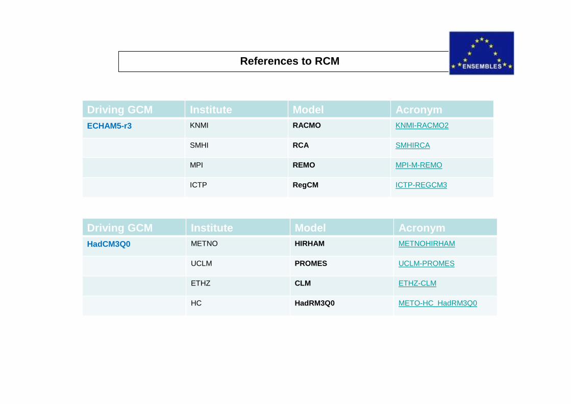
ENSEMBLES project
Considering recent results of the ENSEMBLES project(available at http://ensembles-eu.metoffice.com/ ), two global AOGCM simulations have been used:
�Echam5_r3 (dx*dy= 1.875 x 1.875) (E. Roeckner et. all, 2003:The atmospheric general circulation model ECHAM5Report No. 349OM: Marsland et. all, 2003:The Max-Planck-Institute global ocean/sea ice modelwith orthogonal curvelinearcoordinatesOcean Model., 5, 91-127.OM: Haak, H. et. all, 2003:Formation and propagation of great
salinity anomalies,Geophys. Res. Lett., 30 , 1473,10.1029/2003GL17065)
�HadCM3Q0 (dx*dy= 3.75 x 2.5)(Collins et al, 2006, Clim. Dyn., DOI 10.1007/s00382-006-0121-0)
They have been used for generating a set of RCM (only Atmospheric models).simulations. Some of them covering the whole LMR (Large Mediterranean Region).
This analysis was conducted in the domain following : longitude � from 10 W to 45 Elatitude � from 25 N to 50 N
References to RCM
Driving GCM Institute Model AcronymECHAM5-r3 KNMI RACMO KNMI-RACMO2
SMHI RCA SMHIRCA
MPI REMO MPI-M-REMO
ICTP RegCM ICTP-REGCM3
Driving GCM Institute Model AcronymHadCM3Q0 METNO HIRHAM METNOHIRHAM
UCLM PROMES UCLM-PROMES
ETHZ CLM ETHZ-CLM
HC HadRM3Q0 METO-HC_HadRM3Q0
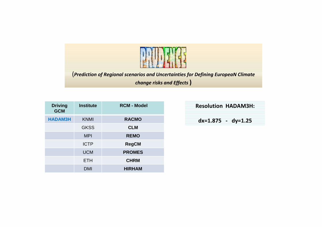
(Prediction of Regional scenarios and Uncertainties for Defining EuropeaN Climate
change risks and Effects )
DrivingGCM
Institute RCM - Model
HADAM3H KNMI RACMO
GKSS CLM
MPI REMO
ICTP RegCM
UCM PROMES
ETH CHRM
DMI HIRHAM
Resolution HADAM3H:
dx=1.875 - dy=1.25

As a Validation we use :
CRU dataset
ERSST dataset
NOCS dataset
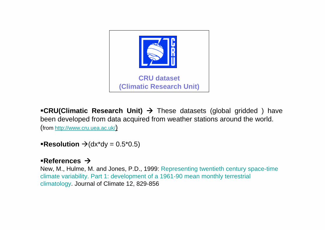
�CRU(Climatic Research Unit) ���� These datasets (global gridded ) have been developed from data acquired from weather stations around the world.(from http://www.cru.uea.ac.uk/)
�Resolution �(dx*dy = 0.5*0.5)
�References ����
New, M., Hulme, M. and Jones, P.D., 1999: Representing twentieth century space-timeclimate variability. Part 1: development of a 1961-90 mean monthly terrestrialclimatology. Journal of Climate 12, 829-856
CRU dataset(Climatic Research Unit)
ERSST dataset( Extended Reconstruction Sea Surface Temperature - version v3b)
�ERSST.v3b is generated using in situ SST data and improved statistical methods that allow stable reconstruction using sparse data.(from http://lwf.ncdc.noaa.gov/oa/climate/research/sst/ersstv3.php )
�Resolution � 2 degree
�References �
Smith, T.M., and R.W. Reynolds, 2003: Extended Reconstruction of Global Sea SurfaceTemperatures Based on COADS Data (1854-1997). Journal of Climate, 16, 1495-1510.ERSST.v2Smith, T.M., and R.W. Reynolds, 2004: Improved Extended Reconstruction of SST (1854-1997). Journal of Climate, 17, 2466-2477.ERSST.v3Smith, T.M., R.W. Reynolds, Thomas C. Peterson, and Jay Lawrimore, 2008: Improvements toNOAA's Historical Merged Land-Ocean Surface Temperature Analysis (1880-2006). Journal ofClimate,21, 2283-2296.Xue, Y., T. M. Smith, and R. W. Reynolds, 2003: Interdecadal changes of 30-yr SST normals during1871-2000. J. Climate, 16, 1601-1612.

NOCS dataset( National Oceanography Centre Southampton)
�NOC1.1 climatology corresponds to the earlier Original SOC flux climatology. The quality of the fields has a strong spatial dependence which reflects the global distribution of ship observations, The fields have been derived from the COADS1a (1980-93) dataset enhanced with additional metadata from the WMO47 list of ships. (from http://www.noc.soton.ac.uk/JRD/MET/fluxclimatology.html )
�Resolution � 1 degree
�References �
Josey, S. A., E. C. Kent and P. K. Taylor, 1998, The Southampton OceanographyCentre (SOC) Ocean-Atmosphere Heat, Momentum and Freshwater Flux Atlas.Southampton Oceanography Centre Rep. 6, Southampton, UK, 30pp .Josey, S. A., E. C. Kent and P. K. Taylor, 1999 , New insights into the ocean heat budget closure problem from analysis of the SOC air-sea flux climatology.Journal of Climate, 12, 2856-2880.
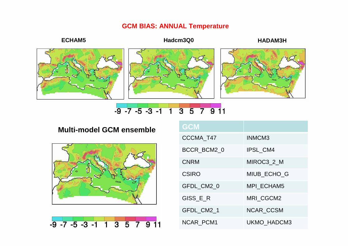
GCM BIAS: ANNUAL Temperature
ECHAM5 Hadcm3Q0 HADAM3H
GCMCCCMA_T47 INMCM3
BCCR_BCM2_0 IPSL_CM4
CNRM MIROC3_2_M
CSIRO MIUB_ECHO_G
GFDL_CM2_0 MPI_ECHAM5
GISS_E_R MRI_CGCM2
GFDL_CM2_1 NCAR_CCSM
NCAR_PCM1 UKMO_HADCM3
Multi-model GCM ensemble

GCM BIAS : ANNUAL PrecipitationECHAM5 Hadcm3Q0 HADAM3H
GCMCCCMA_T47 INMCM3
BCCR_BCM2_0 IPSL_CM4
CNRM MIROC3_2_M
CSIRO MIUB_ECHO_G
GFDL_CM2_0 MPI_ECHAM5
GISS_E_R MRI_CGCM2
GFDL_CM2_1 NCAR_CCSM
NCAR_PCM1 UKMO_HADCM3
Multi-model GCM ensemble
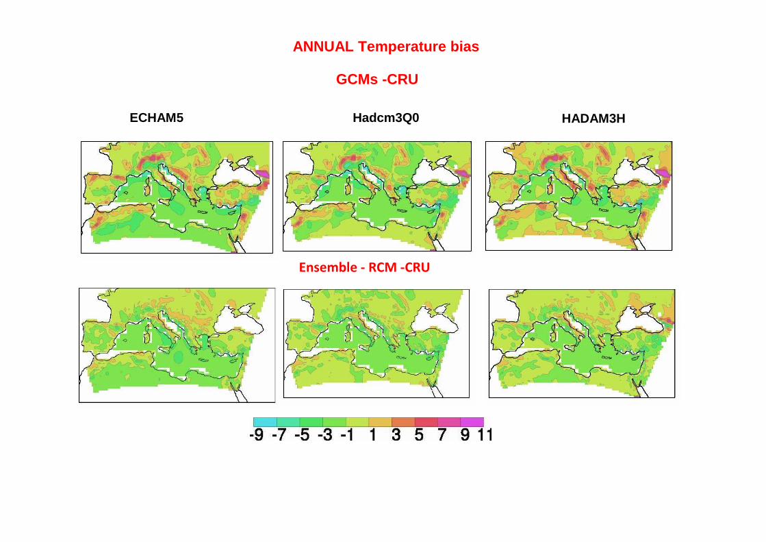
GCMs -CRU
ECHAM5 Hadcm3Q0 HADAM3H
Ensemble - RCM -CRU
ANNUAL Temperature bias
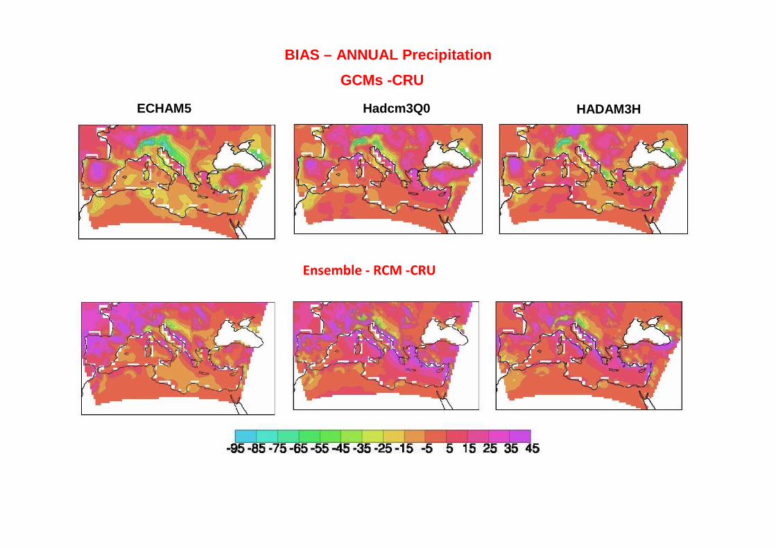
BIAS – ANNUAL Precipitation
ECHAM5 Hadcm3Q0 HADAM3H
GCMs -CRU
Ensemble - RCM -CRU
Echam5 –cru
Ensemble Echam5- CRU
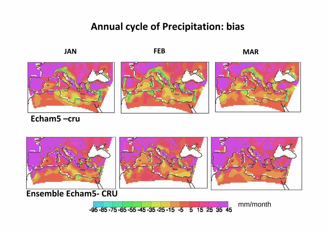
Annual cycle of Precipitation: bias
mm/month
JAN FEB MAR
Echam5 –cru
Ensemble Echam5- CRU
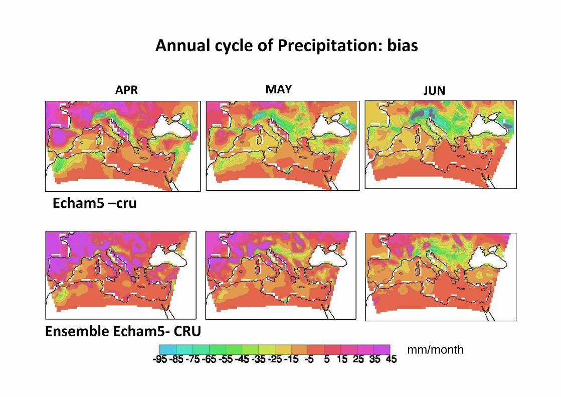
Annual cycle of Precipitation: bias
mm/month
APR MAY JUN

Echam5 –cru
Ensemble Echam5- CRU
Annual cycle of Precipitation: bias
mm/month
JUL AUG SEP
Echam5 –cru
Ensemble Echam5- CRU
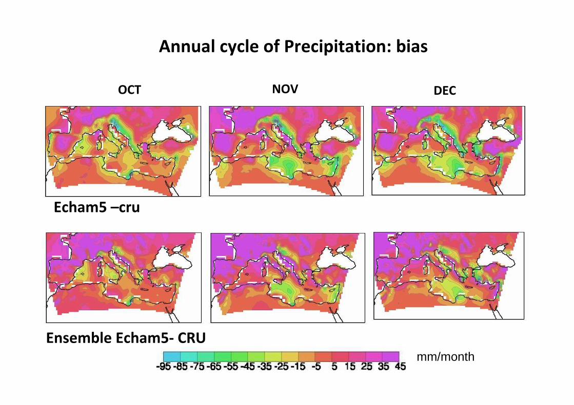
Annual cycle of Precipitation: bias
mm/month
OCT NOV DEC

Sea
b. Land
Land
Hadcm3Q0 Echam5 HADAM3H
GCM
RCM
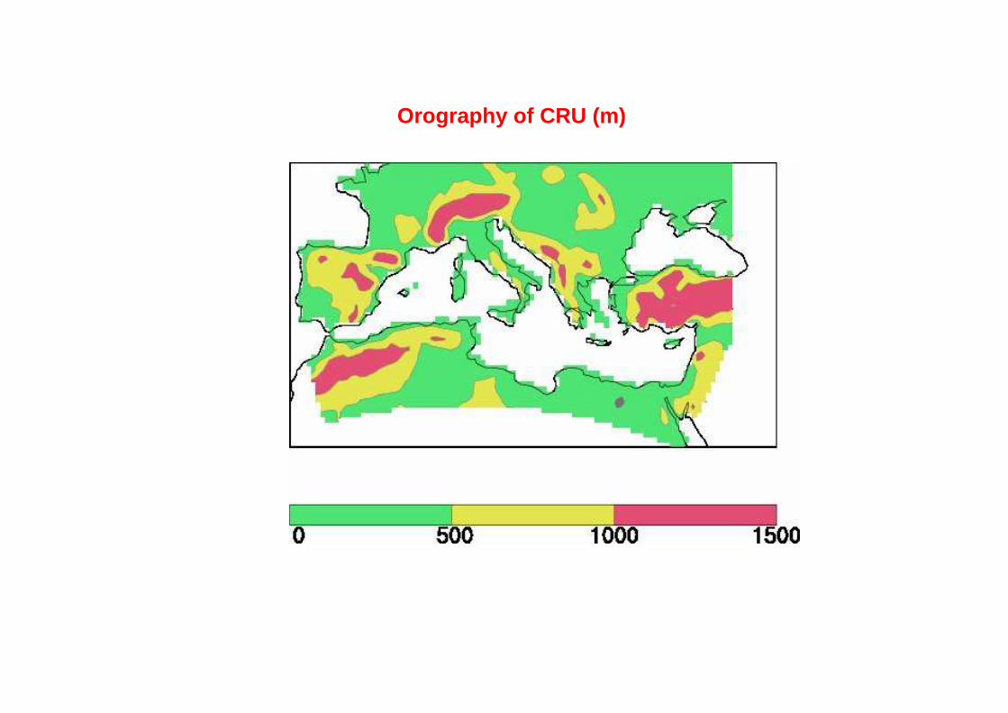
Orography of CRU (m)

Areas at Elevation > 1200(no Turkey)
Coastal LAND areas
Hadcm3Q0 Echam5 HADAM3H
GCM
RCM
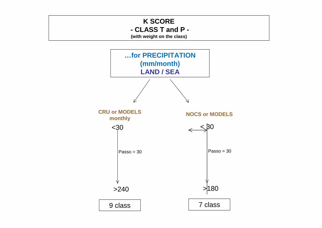
K SCORE- CLASS T and P -(with weight on the class)
…for PRECIPITATION (mm/month)LAND / SEA
CRU or MODELSmonthly
<30
>240
Passo = 30
9 class
NOCS or MODELS
< 30
>180
Passo = 30
7 class
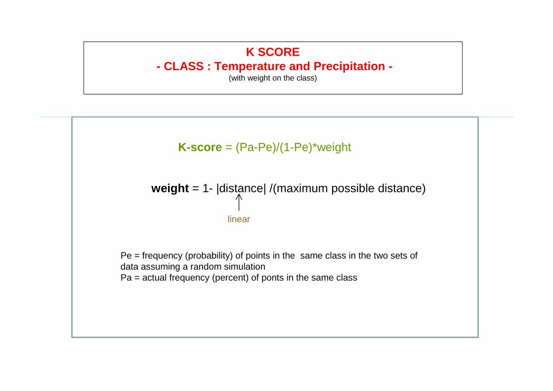
K SCORE- CLASS : Temperature and Precipitation -
(with weight on the class)
Pe = frequency (probability) of points in the same class in the two sets ofdata assuming a random simulationPa = actual frequency (percent) of ponts in the same class
K-score = (Pa-Pe)/(1-Pe)*weight
weight = 1- |distance| /(maximum possible distance)
linear

Annual cycle of K SCORE CRU versus RCM ensembles and /GCMs
Echam5HadCM3Q0
HADAM3H
Ens-Echam5
Ens-HadCM3Q0
Ens- HADAM3H
LAND
SEA

CRU or MODELS(annual)
<300
>750
Passo = 50
11 class
0.430.430.360.490.450.41
HADAM3HHadCM3Q0ECHAM5Ensemble HADAM3H
Ensemble HadCM3Q0
Ensemble ECHAM5
0.270.290.300.270.200.34
HADAM3HHadCM3Q0ECHAM5Ensemble HADAM3H
Ensemble HadCM3Q0
Ensemble ECHAM5
K SCORE ANNUAL– PRECIPITATION: CRU versus models
LAND
SEA

Comparing precipitation fields against CRU 1961-1990 climatology, RCMs score better than GCMs
Improvements are clear in the coastal zone and at high levels
However, these improvements are partially compensated by positive biases introduced in other areas, especially in the period from nov to jan and in the North western corner of the LMR
Therefore the overall score of RCMs is not as higher as one might expect with respect to that of GCMs
All conclusions above hold over land. At the moment, very uncertain conclusions over sea
Conclusions:Conclusions: