do schools in rural and nonrural districts allocate
TRANSCRIPT

I S S U E S & A N S W E R S R E L 2 0 1 1 – N o . 0 9 9
At WestEd
Do schools in rural and nonrural districts allocate resources differently? An analysis of spending and staffing patterns in the West Region states
I S S U E S&ANSWERS R E L 2 0 11 – N o . 0 9 9
At WestEd
Do schools in rural and nonrural districts allocate resources differently? An analysis of spending and staffing patterns in the West Region states
January 2011
Prepared by
Jesse Levin American Institutes for Research
Karen Manship American Institutes for Research
Jay Chambers American Institutes for Research
Jerry Johnson Ohio University
Charles Blankenship American Institutes for Research

WA
OR
ID
MT
NV
CA
UT
AZ
WY
ND
SD
NE
KSCO
NM
TX
OK
CO
AR
LA
MS AL GA
SC
NC
VAWV
KY
TN
PA
NY
FL
AK
MN
WI
IA
IL IN
MI
OH
VT
NH
ME
MO
At WestEd
Issues & Answers is an ongoing series of reports from short-term Fast Response Projects conducted by the regional educa-tional laboratories on current education issues of importance at local, state, and regional levels. Fast Response Project topics change to reflect new issues, as identified through lab outreach and requests for assistance from policymakers and educa-tors at state and local levels and from communities, businesses, parents, families, and youth. All Issues & Answers reports meet Institute of Education Sciences standards for scientifically valid research.
January 2011
This report was prepared for the Institute of Education Sciences (IES) under Contract ED-06-CO-0014 by Regional Edu-cational Laboratory West administered by WestEd. The content of the publication does not necessarily reflect the views or policies of IES or the U.S. Department of Education nor does mention of trade names, commercial products, or organiza-tions imply endorsement by the U.S. Government.
This report is in the public domain. While permission to reprint this publication is not necessary, it should be cited as:
Levin, J., Manship, K., Chambers, J., Johnson, J., and Blankenship, C. (2011). Do schools in rural and nonrural districts allocate resources differently? An analysis of spending and staffing patterns in the West Region states. (Issues & Answers Report, REL 2011–No. 099). Washington, DC: U.S. Department of Education, Institute of Education Sciences, National Center for Education Evaluation and Regional Assistance, Regional Educational Laboratory West. Retrieved from http://ies.ed.gov/ncee/edlabs.
This report is available on the regional educational laboratory web site at http://ies.ed.gov/ncee/edlabs.

Summary
Do schools in rural and nonrural districts allocate resources differently? An analysis of spending and staffing patterns in the West Region states
REL 2011–No. 099
This study of differences in resource allocation between rural and nonrural districts finds that rural districts in the West Region spent more per student, hired more staff per 100 students, and had higher overhead ratios of district- to school-level resources than did city and suburban districts. Regional charac-teristics were more strongly related to resource allocation than were other cost factors studied.
Much of the education finance literature suggests that rural districts face specific challenges—not necessarily faced by their nonrural counterparts—that are thought to affect expenditures. Referred to as cost fac-tors, these challenges include higher costs per student due to the comparatively small scale of operation, higher levels of student need, and difficulty hiring qualified and specialized staff (Duncombe and Yinger 2008). In 2005/06, rural school districts accounted for 43 percent of all districts and served 6 percent of the stu-dent population in the West Region (Arizona, California, Nevada, and Utah).
This report presents the first detailed compari-son of resource allocation between rural and nonrural districts in the West Region. Three regional characteristics often associated with
rural districts were chosen for the analysis: district enrollment, student population density within a district (students per square mile), and drive time from the center of a district to the nearest urban area/cluster. Two other types of factors thought to be associated with resource allocation were also investigated: stu-dent need (incidence of poverty, English lan-guage learner students, and students receiving special education services) and geographic differences in labor costs.
The report first examines how average regional characteristics, student needs, and labor costs differed across rural and nonrural district locale categories in 2005/06. Next it analyzes how average measures of resource alloca-tion (per student expenditures on instruc-tion, administration and student support, and transportation; ratios of administrative, instructional, and student support staff to students; and ratios of district central admin-istration and maintenance and operations spending to school-level spending) varied across district locale categories. Using regres-sion analysis, the study then models how these measures of resource allocation varied with the three regional characteristics and whether the relationship between resource allocation and regional characteristics differed across the study states.
ii Summary
Specifically, the study attempts to answer the following research questions:
• How do factors thought to be related to education costs—such as regional charac-teristics (district enrollment, student pop-ulation density, and proximity to urban areas); student needs (incidence of poverty, English language learner students, and special education enrollment); and labor costs—differ between school districts in rural and nonrural locale categories?
• How do measures of K–12 education resource allocation—including total per student expenditures, staffing ratios, and overhead ratios of district- to school-level spending —differ between school districts in rural and nonrural locale categories?
• How do regional characteristics, student needs, and geographic differences in labor costs relate to patterns of K–12 education spending and staffing in school districts?
The following are key findings of the study:
• Statistically significant differences in en-rollment, student population density, and average drive time to the nearest urban area/cluster were evident in rural and non-rural locales in the West Region. Districts in rural-remote and rural-distant locales (the two most rural district locale sub-categories defined by the National Center for Education Statistics) had substantially lower enrollments and student population densities than did districts in other locale subcategories (ranging on average from fewer than 4 students per square mile
for districts in the two most rural locale categories to more than 400 students per square mile in urban locales).
• Compared with districts in nonrural lo-cales, districts in rural locales spent more per student, hired more staff (especially teachers) per 100 students, and had higher overhead ratios of district- to school-level spending. Of the three regional charac-teristics studied, district enrollment was most strongly related to higher resource utilization.
• Regional characteristics (district enroll-ment, student population density, and drive time) were more strongly related to resource allocation than were other cost factors studied (student needs and geographic differences in labor costs). Longer drive times to urban areas were associated with higher overall per student expenditure; per student expenditures on instruction, administration and student support, and transportation; teacher and administrative staffing ratios; and over-head ratios. Low student population den-sity was significantly related to overall per student expenditure, per student expen-diture on transportation, administrative staffing ratios, and overhead ratios. The magnitude of the differences in resource utilization associated with drive time and student population density was small com-pared with that associated with district enrollment.
Policymakers may want to consider these findings in developing resource distribution formulas and policies.

Requests for this study stemmed from a range of stakeholders, including legislators, educators, and school board members. In California, staff from the State Board of Edu-cation asked for this analysis to better un-derstand how state funding policies play out in rural communities. California legislators requested this analysis to inform resource al-location decisions. Leaders in Nevada’s higher education system requested this analysis to help them understand the resource and cost issues rural communities face. The Direc-tor of the Southwest Comprehensive Center, funded by the U.S. Department of Education,
confirmed that this study would inform mul-tiple ongoing conversations in Arizona and Utah on the unique needs of the many rural districts in those states and that it would be particularly valuable given tight state and local budgets. A 2008 needs survey by the Regional Educational Laboratory West (also funded by the U.S. Department of Educa-tion) indicated that 46 percent of school- and district-level respondents in rural locales reported that “finance” was critical to im-proving their schools.
January 2011
Summary iii
iv Table of conTenTS
TAble of conTenTs
Why this study? 1Regional need 1What the literature shows 2
Current study 4Research questions 4Study conceptual framework 5
Study findings 7How do regional characteristics, student needs, and labor costs differ between school districts in rural and
nonrural locale categories? 9How do measures of education resource allocation differ between school districts in rural and nonrural locale
categories? 11How do regional characteristics, student needs, and geographical differences in labor costs relate to patterns
of education spending and staffing in school districts? 13
Study limitations 22
Policy considerations and direction for future research 23
Appendix A Distribution of school districts and students in West Region states by locale category, 2005/06 24
Appendix B Data sources and variable construction 26
Appendix C Modifications made to raw Common Core of Data and School District Finance Survey data files 31
Appendix D Results of pair-wise comparisons for district locales 32
Appendix E Missing and recoded records and variables 48
Appendix F Regression analysis methodology and models 50
Appendix G Regression model results 53
Notes 61
References 62
Boxes
1 Data sources and analysis 6
B1 Creation of the drive time metric 29
Figures
1 Simple framework for district resource allocation 5
2 Average district enrollment, student population density, drive time to nearest urban area/cluster, and labor costs in districts in West Region states by locale category, 2005/06 10
3 Average student need levels of districts in West Region states by locale category, 2005/06 10

Table of conTenTS v
4 Average per student expenditures by districts in West Region states by locale category, 2005/06 11
5 Average per student expenditures on instruction, administration and student support, and transportation by districts in West Region states by locale category, 2005/06 12
6 Average staffing ratios for districts in West Region states by locale category, 2005/06 13
7 Average overhead ratios for districts in West Region states by locale category, 2005/06 14
8 Estimated relationship between overall per student expenditures and enrollment in Arizona and California, 2005/06 16
9 Estimated relationship between per student instruction expenditures and enrollment in Arizona, California, and Utah, 2005/06 16
10 Estimated relationship between per student administration and student support expenditure and enrollment in Arizona, California, and Utah, 2005/06 16
11 Estimated relationship between per student transportation expenditures and enrollment in California, 2005/06 16
12 Estimated relationship between overall per student expenditures and student population density in California, 2005/06 17
13 Estimated relationship between per student transportation expenditures and student population density in California, 2005/06 17
14 Estimated relationship between overall per student expenditure and drive time to nearest urban area/cluster in California, 2005/06 18
15 Estimated relationship between per student instruction expenditures and drive time to nearest urban area/cluster in California, 2005/06 18
16 Estimated relationship between per student administration and student support expenditure and drive time to nearest urban area/cluster in California, 2005/06 18
17 Estimated relationship between teacher staffing ratio and enrollment in Arizona, California, and Utah, 2005/06 19
18 Estimated relationship between administrator staffing ratio and enrollment in Arizona, California, and Utah, 2005/06 19
19 Estimated relationship between administrator staffing ratio and student population density in California, 2005/06 20
20 Estimated relationship between teacher staffing ratio and drive time to nearest urban area/cluster in California, 2005/06 20
21 Estimated relationship between administrator staffing ratio and drive time to nearest urban area/cluster in California, 2005/06 20
22 Estimated relationship between overall overhead ratio and enrollment in California, 2005/06 21
23 Estimated relationship between overall overhead ratio and student population density in California, 2005/06 22
vi Table of conTenTS
24 Estimated relationship between overall overhead ratio and drive time to nearest urban area/cluster in California, 2005/06 22
Tables
1 Distribution of school districts and students in West Region states by four National Center for Education Statistics locale categories, 2005/06 2
2 Distribution of school districts and students in West Region states by seven National Center for Education Statistics locale categories, 2005/06 9
3 Regression results: statistically significant relationships between regional characteristics and per student expenditures in California, Arizona, and Utah, 2005/06 15
4 Regression results: statistically significant relationships between regional characteristics and staffing ratios in California, Arizona, and Utah, 2005/06 19
5 Regression results: statistically significant relationships between regional characteristics and overhead ratios in California, Arizona, and Utah, 2005/06 21
A1 Distribution of school districts in West Region states by locale category, 2005/06 24
A2 Distribution of students in West Region states by locale category, 2005/06 25
B1 Sources of study data 26
B2 Aggregation of National Center for Education Statistics locale codes for use in this study 28
C1 West Region districts listed as unified in the School District Finance Survey but separate in the Common Core of Data 31
D1 Means, standard deviations, and significant indicators for t-tests comparing contextual variables in nonrural and rural school district locales in all districts in study, 2005/06 32
D2 Means, standard deviations, and significant indicators for t-tests comparing expenditure categories in nonrural and rural school district locales in all districts in study, 2005/06 33
D3 Means, standard deviations, and significant indicators for t-tests comparing contextual variables in nonrural and rural school district locales in Arizona, 2005/06 35
D4 Means, standard deviations, and significant indicators for t-tests comparing expenditure categories in nonrural and rural school district locales in Arizona, 2005/06 36
D5 Means, standard deviations, and significant indicators for t-tests comparing contextual variables in nonrural and rural school district locales in California, 2005/06 38
D6 Means, standard deviations, and significant indicators for t-tests comparing expenditure categories in nonrural and rural school district locales in California, 2005/06 39
D7 Means, standard deviations, and significant indicators for t-tests comparing contextual variables in nonrural and rural school district locales in Nevada, 2005/06 41
D8 Means, standard deviations, and significant indicators for t-tests comparing expenditure categories in nonrural and rural school district locales in Nevada, 2005/06 42

Table of conTenTS vii
D9 Means, standard deviations, and significant indicators for t-tests comparing contextual variables in nonrural and rural school district locales in Utah, 2005/06 44
D10 Means, standard deviations, and significant indicators for t-tests comparing expenditure categories in nonrural and rural school district locales in Utah, 2005/06 45
D11 p-values for nonrural to rural t-test results for all resource measures for all significant differences 46
D12 Locale means standardized relative to overall means and standard deviations for each resource measure 47
E1 Districts and students dropped from analysis of per student transportation expenditures in Arizona and California, 2005/06 48
E2 Districts and students dropped from analysis of teacher staffing ratio in Arizona and California, 2005/06 48
E3 Districts and students dropped from analysis of student support staffing ratio in Arizona and California, 2005/06 49
E4 Districts and students dropped from analysis of administrator staffing ratio in Arizona and California, 2005/06 49
E5 Districts and students dropped from analysis of central administration overhead ratio in Arizona and California, 2005/06 49
F1 Example of predicted differentials in overall per student expenditures associated with district enrollment, 2005/06 51
G1 Development of final regression model using overall per student expenditures in 2005/06 as dependent variable 53
G2 Regressions of per student expenditures in West Region school districts, 2005/06 55
G3 Regressions of staffing ratios in West Region, 2005/06 57
G4 Regressions of overhead ratios in West Region, 2005/06 59

Why ThiS STudy? 1
This study of differences in resource allocation between rural and nonrural districts finds that rural districts in the West Region spent more per student, hired more staff per 100 students, and had higher overhead ratios of district- to school-level resources than did city and suburban districts. Regional characteristics were more strongly related to resource allocation than were other cost factors studied.
Why This sTuDy?
Rural communities face a number of challenges in providing education services that suburban and urban areas do not. The geographic isolation that often defines rural communities forces them to operate schools on a substantially smaller scale than is generally considered fiscally optimal. In addition, because distances between student homes and between student homes and schools are longer, transportation costs in rural districts are often higher. Isolated rural districts also often find it difficult to recruit and retain teachers (Col-lins 1999). This report explores the implications of these challenges.
Regional need
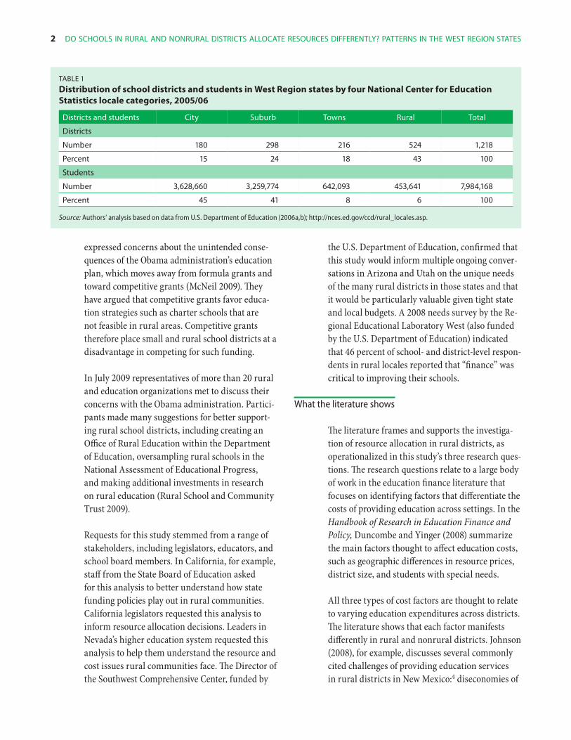
In the 2005/06 school year, 43 percent of districts in the West Region states (Arizona, California, Nevada, and Utah) were classified as rural based on the National Center for Education Statistics (NCES) definitions of locale category (table 1).1 These districts served 453,641 students, 6 percent of the total student population in the region. (Ap-pendix A provides a detailed breakout of both the counts and percentages of districts and students by state and district locale category.)2
Limited research has been conducted on rural education in general; even less has been done on finance and access to education resources in rural areas. To inventory topics covered in the rural education research literature and assess the qual-ity of this research, Arnold et al. (2005) carried out a comprehensive search of the literature on education research referenced in the ERIC and PsycINFO databases from 1991 to 2003. Of 498 articles found, only 9 focused on school finance.3 The study placed education finance among the high-priority topics for the rural education re-search agenda.
Given the recent fiscal crisis facing virtually all states, research on rural education finance is timely. In recent articles in the popular press, policymakers and advocates for rural schools have
2 do SchoolS in rural and nonrural diSTricTS allocaTe reSourceS differenTly? paTTernS in The WeST region STaTeS
Table 1
Distribution of school districts and studestatistics locale categories, 2005/06
nts in West Region states by four national center for education
districts and students city Suburb Towns rural Total
districts
number 180 298 216 524 1,218
percent 15 24 18 43 100
Students
number 3,628,660 3,259,774 642,093 453,641 7,984,168
percent 45 41 8 6 100
Source: Authors’ analysis based on data from U.S. Department of Education (2006a,b); http://nces.ed.gov/ccd/rural_locales.asp.
expressed concerns about the unintended conse-quences of the Obama administration’s education plan, which moves away from formula grants and toward competitive grants (McNeil 2009). They have argued that competitive grants favor educa-tion strategies such as charter schools that are not feasible in rural areas. Competitive grants therefore place small and rural school districts at a disadvantage in competing for such funding.
In July 2009 representatives of more than 20 rural and education organizations met to discuss their concerns with the Obama administration. Partici-pants made many suggestions for better support-ing rural school districts, including creating an Office of Rural Education within the Department of Education, oversampling rural schools in the National Assessment of Educational Progress, and making additional investments in research on rural education (Rural School and Community Trust 2009).
Requests for this study stemmed from a range of stakeholders, including legislators, educators, and school board members. In California, for example, staff from the State Board of Education asked for this analysis to better understand how state funding policies play out in rural communities. California legislators requested this analysis to inform resource allocation decisions. Leaders in Nevada’s higher education system requested this analysis to help them understand the resource and cost issues rural communities face. The Director of the Southwest Comprehensive Center, funded by
the U.S. Department of Education, confirmed that this study would inform multiple ongoing conver-sations in Arizona and Utah on the unique needs of the many rural districts in those states and that it would be particularly valuable given tight state and local budgets. A 2008 needs survey by the Re-gional Educational Laboratory West (also funded by the U.S. Department of Education) indicated that 46 percent of school- and district-level respon-dents in rural locales reported that “finance” was critical to improving their schools.
What the literature shows
The literature frames and supports the investiga-tion of resource allocation in rural districts, as operationalized in this study’s three research ques-tions. The research questions relate to a large body of work in the education finance literature that focuses on identifying factors that differentiate the costs of providing education across settings. In the Handbook of Research in Education Finance and Policy, Duncombe and Yinger (2008) summarize the main factors thought to affect education costs, such as geographic differences in resource prices, district size, and students with special needs.
All three types of cost factors are thought to relate to varying education expenditures across districts. The literature shows that each factor manifests differently in rural and nonrural districts. Johnson (2008), for example, discusses several commonly cited challenges of providing education services in rural districts in New Mexico:4 diseconomies of

Why ThiS STudy? 3
scale because of the small numbers of students and the large areas covered; greater difficulty employ-ing staff, because job markets are more isolated; and disproportionately high rates of students with special needs.
School and district size. Because of the small scale of school and district operations, rural com-munities face challenges in providing the level of education services common in more populated areas. Low enrollments do not permit rural school districts to take full advantage of the economies of scale enjoyed by larger districts. Fixed costs, which vary disproportionately with student enrollment, make it difficult to use resources efficiently, partly explaining the higher cost of education in rural districts.
The need to transport students over long distances is an example of the extraordinary financial pres-sure of low student population density on rural school districts. Killeen and Sipple (2000) show that per student transportation expenditures are about twice as high in rural districts as in urban districts and 50 percent higher than in suburban districts. Longer distances could affect costs both because of the greater number of miles driven and because a higher proportion of children in these communities likely rely on school buses to get to school.
Recruiting and retaining qualified staff. The chal-lenge of operating at a small scale is compounded by the difficulty of attracting qualified staff to remote rural districts. A literature review by Hammer et al. (2005) reveals several contributing factors, including social and geographic isolation, difficult working conditions, and the need to teach multiple subjects. These findings are supported by previous research on geographic variation in the cost of education that shows the cost of obtain-ing comparable teaching staff to be significantly higher in geographically isolated labor markets (Chambers 1995).
Levels of need among rural students. Rural dis-tricts often have disproportionately high levels of students with special needs related to poverty,
mobility, English lan-guage learner status, and special education (John-son and Strange 2009). A regression-based cost function analysis of rural and nonrural districts in Texas and Wisconsin (Imazeki and Rechovsky 2003) provides additional empirical support to the notion that appropriate instruction and related services for students with such special needs require additional and special-ized resources.
National and state studies. Also informing the study is research that considers differences in rural and nonrural spending patterns at the national and state levels. This literature is marked by methodological limitations that the current study attempts to address by accounting for rural-nonrural differences across states and by modeling key characteristics of rurality rather than simply treating it as a categorical variable.
Few studies examine differences between rural and nonrural education finance at the national level. Three national-level government reports on staffing and expenditures across district locales corroborate the finding that rural districts spend more per student than their nonrural counter-parts. Stern (1994), which lists the nationwide average per student expenditure in 1982 for met-ropolitan and nonmetropolitan counties, shows that these expenditures were indeed higher in nonmetropolitan areas. Parrish, Matsumoto, and Fowler (1995) and Provasnik et al. (2007) provide more sophisticated analyses of these differences by controlling for both student needs and regional cost variations in hiring and retaining staff. Both studies report higher average per student expendi-tures in rural districts than in nonrural districts.
The two latter studies thus provide improved measures of the differences in expenditures across rural and nonrural districts. However, because the studies report averages across all rural and
because of the small
scale of school and
district operations,
rural communities face
challenges in providing
the level of education
services common in
more populated areas
4 do SchoolS in rural and nonrural diSTricTS allocaTe reSourceS differenTly? paTTernS in The WeST region STaTeS
nonrural districts in the country, they do not provide insight into whether differences between rural and nonrural expenditures vary by state. Differences between rural and nonrural expenditures and resource allocation would be expected to be at least partially driven by state funding mecha-nisms. Investigating expendi-tures and resource allocation within states is thus a worthwhile endeavor.
State-level studies of rural education finance are limited, and most are descriptive. Maiden and Stearns (2007) identify greater inequity in Okla-homa among rural school districts than among nonrural districts, in both total current expendi-tures and capital expenditures. They also find that rural school districts were more affected by varia-tions in local property wealth than were nonrural districts, possibly because the tax base of many rural school districts depends heavily on agricul-tural land, whose value fluctuates in response to commodity prices (Ward 2003). McLean and Ross (1994) examine education resources and school conditions in Alabama’s highest and lowest funded school districts. They find notable rural-urban dis-parities, which contributed to inadequate facilities, resources, and staffing in rural schools. Using a similar approach, Walters (1996) finds significant rural-urban differences in spending patterns over a 10-year period among Pennsylvania’s 25 highest spending and 25 lowest spending districts.
In most of these studies, rural status serves as a category for comparing average resource alloca-tion. Relationships between resource allocation and continuous measures of rurality such as the regional characteristics used in this study (enroll-ment, student population density, and drive time to nearest urban area) have rarely been examined, especially while controlling for other factors thought to be related to resource use (such as student needs and geographic differences in labor costs). Moreover, few studies have performed a
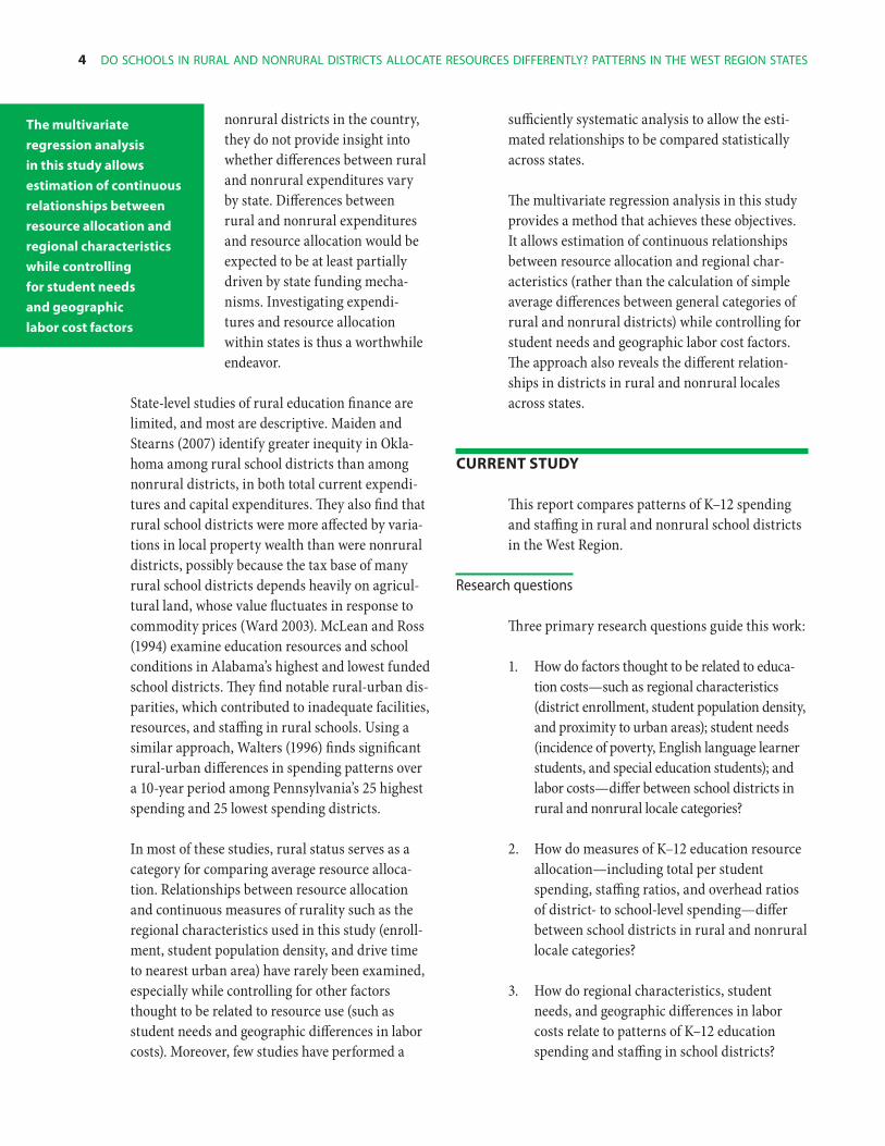
sufficiently systematic analysis to allow the esti-mated relationships to be compared statistically across states.
The multivariate regression analysis in this study provides a method that achieves these objectives. It allows estimation of continuous relationships between resource allocation and regional char-acteristics (rather than the calculation of simple average differences between general categories of rural and nonrural districts) while controlling for student needs and geographic labor cost factors. The approach also reveals the different relation-ships in districts in rural and nonrural locales across states.
cuRRenT sTuDy
This report compares patterns of K–12 spending and staffing in rural and nonrural school districts in the West Region.
Research questions
Three primary research questions guide this work:
1. How do factors thought to be related to educa-tion costs —s uch as regional characteristics (district enrollment, student population density, and proximity to urban areas); student needs (incidence of poverty, English language learner students, and special education students); and labor costs— differ between school districts in rural and nonrural locale categories?
2. How do measures of K–12 education resource allocation—i ncluding total per student spending, staffing ratios, and overhead ratios of district- to school-level spending— differ between school districts in rural and nonrural locale categories?
3. How do regional characteristics, student needs, and geographic differences in labor costs relate to patterns of K–12 education spending and staffing in school districts?
The multivariate
regression analysis
in this study allows
estimation of continuous
relationships between
resource allocation and
regional characteristics
while controlling
for student needs
and geographic
labor cost factors

currenT STudy 5
Resource allocationdecisions
Local fiscal capacity
Local education taxes andrevenues from state
or federal sources
District outcome goals Cost factors
• Regional characteristics(district size andremoteness)
• Student needs
• Geographic differencesin labor costs
figure 1
simple framework for district resource allocation
Source: Authors’ analysis.
Study conceptual framework
The simple conceptual framework shown in figure 1 is useful for understanding resource al-location decisions in rural school districts as they apply to this study. Under this model, after setting goals for student outcomes, districts consider the various cost factors—regional characteristics, student needs, and geographic differences in labor costs:
• Regional characteristics. Geographic and pop-ulation features of a school district, including enrollment (number of students served by a district), student population density (district enrollment divided by the area of the district in square miles), and drive time to the center of the nearest urban area/cluster.
• Student needs. Student characteristics that necessitate additional or specialized services, including poverty, English language learner status, and special education status.
• Geographic differences in labor costs. Differ-ences in the cost of hiring similarly qualified staff across regional labor markets.
These cost factors, combined with local fiscal capacity, local education taxes, and revenues from state and federal sources, determine how much
districts spend and how they allocate spending across resource categories.
Cost factors may affect a district’s outcome goals as well as its fiscal capacity to reach them. With this in mind, the goal of this study is to focus on the relationship between cost factors and patterns of resource utilization (see box 1 on data sources and analysis) rather than to develop a compre-hensive model of this framework that includes all three determinants of resource allocation.
Implicit in resource allocation is the potential impact of cost factors on local fiscal capacity and district outcome goals. There is both theoretical and empirical support for the possibility that these relationships differ across states. Each state has its own tax structure, which affects the composition of state and local tax revenues made available to school districts, and states compensate for these cost factors through different mechanisms in their school fund-ing formulas (Verstegen, Jordan, and Amador 2007). In addition, states have different accommodations in their school funding formulas to compensate for variations in the measures of the regional character-istics, student needs, and geographic differences in labor costs included in this study (see U.S. Depart-ment of Education 2001; Verstegen and Jordan 2009). Such differences, combined with differences in the provisions for compensating for the cost factors in each state, are likely to affect the responsiveness of
6 do SchoolS in rural and nonrural diSTricTS allocaTe reSourceS differenTly? paTTernS in The WeST region STaTeS
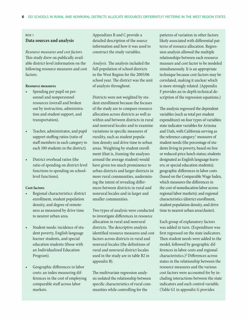
box 1
Data sources and analysis
Resource measures and cost factors. This study drew on publically avail-able district-level information on the following resource measures and cost factors.
Resource measures• Spending per pupil on per-
sonnel and nonpersonnel resources (overall and broken out by instruction, administra-tion and student support, and transportation).
• Teacher, administrator, and pupil support staffing ratios (ratio of staff members in each category to each 100 students in the district).
• District overhead ratios (the ratio of spending on district-level functions to spending on school-level functions).
Cost factors• Regional characteristics: district
enrollment, student population density, and degree of remote-ness as measured by drive time to nearest urban area.
• Student needs: incidence of stu-dent poverty, English language learner students, and special education students (those with an Individualized Education Program).
• Geographic differences in labor costs: an index measuring dif-ferences in the cost of employing comparable staff across labor markets.
Appendixes B and C provide a detailed description of the source information and how it was used to construct the study variables.
Analysis. The analysis included the full population of school districts in the West Region for the 2005/06 school year. The district was the unit of analysis throughout.
Districts were not weighted by stu-dent enrollment because the focuses of the study are to compare resource allocation across districts as well as within and between districts in rural and nonrural locales and to examine variations in specific measures of rurality, such as student popula-tion density and drive time to urban areas. Weighting by student enroll-ment (that is, framing the analyses around the average student) would have given too much prominence to urban districts and larger districts in more rural communities, undermin-ing the intent of revealing differ-ences between districts in rural and nonrural locales and in larger and smaller communities.
Two types of analysis were conducted to investigate differences in resource allocation in rural and nonrural districts. The descriptive analysis identified resource measures and cost factors across districts in rural and nonrural locales (the definitions of rural and nonrural district locales used in the study are in table B2 in appendix B).
The multivariate regression analy-sis isolated the relationship between specific characteristics of rural com-munities while controlling for the
patterns of variation in other factors likely associated with differential pat-terns of resource allocation. Regres-sion analysis allowed the multiple relationships between each resource measure and cost factor to be modeled simultaneously. It is an appropriate technique because cost factors may be correlated, making it unclear which is more strongly related. (Appendix F provides an in-depth technical de-scription of the regression equations.)
The analysis regressed the dependent variables (such as total per student expenditure) on four types of variables: state indicator variables for Arizona and Utah, with California serving as the reference category;1 measures of student needs (the percentage of stu-dents living in poverty, based on free or reduced-price lunch status; students designated as English language learn-ers; or special education students); geographic differences in labor costs (based on the Comparable Wage Index, which measures the differences in the cost of noneducation labor across regional labor markets); and regional characteristics (district enrollment, student population density, and drive time to nearest urban area/cluster).
Each group of explanatory factors was added in turn. (Expenditure was first regressed on the state indicators. Then student needs were added to the model, followed by geographic dif-ferences in labor costs and regional characteristics.)2 Differences across states in the relationship between the resource measures and the various cost factors were accounted for by in-cluding interactions between the state indicators and each control variable. (Table G1 in appendix G provides
(conTinued)
study Findings 7
Box 1 (Continued)
Data sources and analysis
the detailed results of the regressions leading to the final model.)
The estimated models were then used to simulate patterns of variation in the resource measures associated with each regional characteristic while holding all other cost factors constant at their sample means. In this way, it was possible to isolate the relation-ship between resource allocation and regional characteristics (for example,
the relationship between per student expenditure and enrollment).
Note1. Nevada was excluded from these multi-
variate analyses because the small num-ber of school districts (17) in the state made it impossible to reliably estimate model parameters.
2. A log-linear functional form was adopted in which logarithmic transformations of the resource measures (dependent variables) and cost factors (independent variables) related to student needs (district
percentages of students in poverty, Eng-lish language learner students, and special education students) and selected regional characteristics (district enrollment and student population density) were used. Logarithmic transformations were in-cluded to provide estimated proportional (nonlinear) relationships between the cost factors and the resource measures. These types of estimated relationships are regularly measured by economists, who refer to them as elasticities. For a detailed technical description of the final regres-sion model, see appendix F.
patterns of resource allocation to these cost factors, through the mechanisms that influence the way local boards and school decisionmakers set local tax rates and determine how best to allocate revenues to various school inputs (see Chambers 1979).
Study findingS
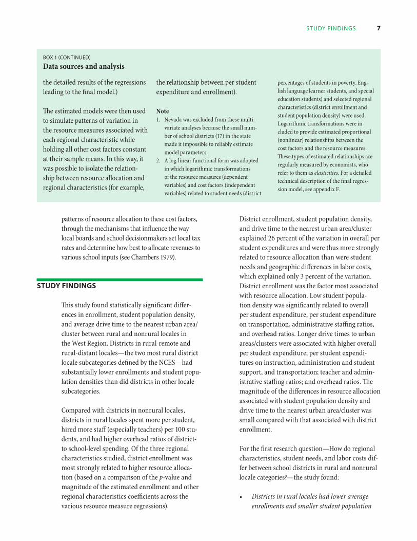
This study found statistically significant differ-ences in enrollment, student population density, and average drive time to the nearest urban area/cluster between rural and nonrural locales in the West Region. Districts in rural-remote and rural-distant locales —t he two most rural district locale subcategories defined by the NCES — had substantially lower enrollments and student popu-lation densities than did districts in other locale subcategories.
Compared with districts in nonrural locales, districts in rural locales spent more per student, hired more staff (especially teachers) per 100 stu-dents, and had higher overhead ratios of district- to school-level spending. Of the three regional characteristics studied, district enrollment was most strongly related to higher resource alloca-tion (based on a comparison of the p-value and magnitude of the estimated enrollment and other regional characteristics coefficients across the various resource measure regressions).
District enrollment, student population density, and drive time to the nearest urban area/cluster explained 26 percent of the variation in overall per student expenditures and were thus more strongly related to resource allocation than were student needs and geographic differences in labor costs, which explained only 3 percent of the variation. District enrollment was the factor most associated with resource allocation. Low student popula-tion density was significantly related to overall per student expenditure, per student expenditure on transportation, administrative staffing ratios, and overhead ratios. Longer drive times to urban areas/clusters were associated with higher overall per student expenditure; per student expendi-tures on instruction, administration and student support, and transportation; teacher and admin-istrative staffing ratios; and overhead ratios. The magnitude of the differences in resource allocation associated with student population density and drive time to the nearest urban area/cluster was small compared with that associated with district enrollment.
For the first research question — How do regional characteristics, student needs, and labor costs dif-fer between school districts in rural and nonrural locale categories?— the study found:
• Districts in rural locales had lower average enrollments and smaller student population

8 do sChools in rural and nonrural distriCts alloCate resourCes diFFerently? patterns in the West region states
densities than did districts in more urban locales in the West Region states.5 Districts in the four most rural district locale subcategories (rural-remote, rural-distant, rural-fringe, and town-remote) had lower average enrollments than did districts in other locale cat-egories (city, suburb, town-fringe, and town-distant). Rural-remote and rural-distant districts had sig-nificantly smaller student popula-
tion densities than did districts in all other locale categories, ranging from fewer than 4 students per square mile for rural-remote and rural-distant districts to more than 400 per square mile for city districts.
• The drive from the center of the district to the nearest urban area/cluster was longer on aver-age in rural-remote and rural-distant locales than in districts in other locales (city, suburb, town-fringe, and town-distant). Rural-remote districts had the longest drive time to the nearest urban area, but because of how locale subcategories are defined (by distance to Census-defined urban areas/clusters), average drive time is lower for rural-fringe and town-remote districts than for suburban districts.
• Poverty was highest in rural-remote districts, but nonrural locale categories had the highest average levels of other student needs such as proportions of English language learner students and students who qualify for special education services. City districts had the larg-est average proportion of English language learner students, but such students were enrolled in smaller proportions in districts in all rural locale categories. The largest aver-age proportion of special education students was in town-remote districts, followed by rural-remote locales. Poverty was highest in rural-remote districts, followed by town-remote and town-not remote districts. In contrast to findings of nationwide studies, the results here show that student needs in the
West Region were not consistently higher in rural districts.
For the second research question — How does edu-cation resource allocation differ between school districts in rural and nonrural locale categories? — the study found:
• Rural districts used more resources per student and had higher overhead than did nonrural districts in the West Region. Compared with nonrural school districts, rural school districts spent more per student (on instruction, admin-istration and student support, transportation, and overall); hired more staff (especially teach-ers) per 100 students; and had higher overhead ratios of district- to school-level resources.
For the third research question — How do regional characteristics, student needs, and geographic dif-ferences in labor costs relate to patterns of educa-tion spending and staffing in school districts? — the study found:
• Districts with lower enrollments, lower student population densities, and longer drive times to urban areas/clusters spent more per student, hired more staff per 100 students, and had higher overhead ratios. The estimated rela-tionships between enrollment and education resource allocation (spending and staffing pat-terns) were statistically significant: districts with lower enrollments spent more per stu-dent and hired more staff per 100 students. In general, lower student population density in a district appeared to be associated with higher resource allocation per student (higher per student expenditures overall, as well as higher per student expenditures on transportation, administrator staffing ratios, and overhead ratios). Longer drive time to an urban area/cluster was associated with higher per student expenditures overall, as well as higher per stu-dent expenditures on instruction, administra-tion and student support, and transportation; higher teacher and administrative staffing ratios; and higher overhead ratios.
districts with lower
enrollments, lower
student population
densities, and longer
drive times to urban
areas/clusters spent
more per student,
hired more staff per
100 students, and had
higher overhead ratios

STudy findingS 9
• Among regional characteristics, district enroll-ment was most strongly related to resource allocation. Differences in spending associated with student population density and drive time to the nearest urban area/cluster were much smaller than those associated with district enrollment.
The following sections describe the findings for the three research questions in greater detail.
How do regional characteristics, student needs, and labor costs differ between school districts in rural and nonrural locale categories?
Districts were classified into the four most rural (rural-remote, rural-distant, rural-fringe, and town-remote) and three nonrural NCES locale categories and subcategories (see appendix B). The four most rural district locale categories accounted for 49 percent of the districts and 8 percent of students in the West Region (table 2). Districts in the two most rural locale categories (rural-distant and rural-remote) accounted for 29 percent of the districts in the region and 2 percent of all students.
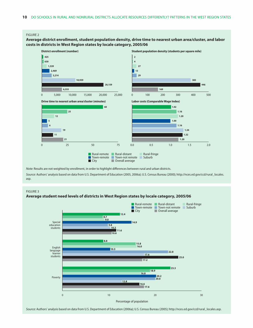
Differences in regional characteristics. As expected, enrollment and student population density were higher in city and suburban districts than in rural districts (figure 2).6 Not surprisingly, average drive time to the nearest urban area/cluster was longest in rural-remote and rural-distant districts. The
next longest drive time to urban areas/clusters was in suburban districts, however.
This counterintuitive result is an artifact of the method used to define locale categories. Towns exist in urban clusters, which are typically smaller than urban areas; as drive times were calculated to the nearest urban area/cluster, the shortest times were seen in town-remote and town-not remote districts. In contrast, suburban districts, which are often on the outskirts of larger urban areas, had longer drive times than all but the two most re-mote locale categories. It could be argued that this finding, which seems to call into question the use of drive time as an explanatory variable, actually provides information lacking in the NCES locale typology (http://nces.ed.gov/ccd/rural_locales.asp). Drive time to the closest urban area/cluster provides a continuous measure of remoteness that is more meaningful than straight-line distance. Knowing, for instance, that driving to an urban area/cluster from a rural-remote district takes twice as long as from a rural-distant district is valuable when examining cost patterns associated with rural education.
Differences in student needs. The relationship between student needs and district locale in the West Region states was less clearly defined than the literature suggests. In the districts included in the analysis, there was no obvious relationship be-tween district locale and the percentage of special
Table 2
Distribution of school districts and students in West Region states by seven national center for edstatistics locale categories, 2005/06
ucation
districts and Town- Town- rural- rural- rural-students city Suburb not remote remote fringe distant remote Total
districts
number 180 298 146 70 173 186 165 1,218
percent 15 24 12 6 14 15 14 100
Students
number 3,628,660 3,259,774 469,242 172,851 266,303 117,209 70,129 7,984,168
percent 45 41 6 2 3 1 1 100
Note: Percentages are rounded to whole numbers, so rural locale subcategories may not sum to the rural locale category totals in table 1.
Source: Authors’ analysis based on data from U.S. Department of Education (2006a); http://nces.ed.gov/ccd/rural_locales.asp.
10 do SchoolS in rural and nonrural diSTricTS allocaTe reSourceS differenTly? paTTernS in The WeST region STaTeS
Rural-remote Rural-distant Rural-fringeTown-remote Town-not remote SuburbCity Overall average
0 5,000 10,000 15,000 20,000 25,000
District enrollment (number)
Drive time to nearest urban area/cluster (minutes)
0 100 200 300 400 500
Student population density (students per square mile)
Labor costs (Comparable Wage Index)
0 25 50 75 0.0 0.5 1.0 1.5 2.0
425
630
1,539
2,469
3,214
20,159
10,939
6,555
60
25
12
5
6
11
19
21
2
4
27
13
29
446
383
169
1.02
1.16
1.20
1.00
1.16
1.32
1.34
1.20
figure 2
Average district enrollment, student population density, drive time to nearest urban area/cluster, and labor costs in districts in West Region states by locale category, 2005/06
Note: Results are not weighted by enrollment, in order to highlight differences between rural and urban districts.
Source: Authors’ analysis based on data from U.S. Department of Education (2005, 2006a); U.S. Census Bureau (2000); http://nces.ed.gov/ccd/rural_locales.asp.
0 10 20 30
Percentage of population
Rural-remote Rural-distant Rural-fringeTown-remote Town-not remote SuburbCity Overall average
Poverty
Englishlanguage
learnerstudents
Specialeducation
students
12.48.7
9.014.9
9.810.3
11.610.6
25.017.6
22.810.3
16.015.8
8.8
17.2
16.612.8
20.020.2
16.818.9
23.3
17.6
figure 3
Average student need levels of districts in West Region states by locale category, 2005/06
Source: Authors’ analysis based on data from U.S. Department of Education (2006a); U.S. Census Bureau (2005); http://nces.ed.gov/ccd/rural_locales.asp.
STudy findingS 11
education students (that is, students with an Individualized Education Program). Rural-remote, town-remote, and city districts served higher than average proportions of special education students, but rural-distant districts had the smallest per-centage of such students (figure 3).
The percentage of English language learner stu-dents varied by district locale. In the four rural locale categories, their proportion was below the regional average of 17 percent; districts in rural-remote locales had the smallest proportion, at 9 percent. The proportions of English language learner students in the three nonrural locale categories were above the regional average, with city districts having the highest concentrations, at 25 percent.
The percentage of students living in poverty also varied by locale category. The highest proportion was in rural-remote locales (23 percent); the lowest was in suburban locales (13 percent). However, districts in town locales had higher percentages of students living in poverty (20 percent in town-remote and 20 percent in town-not remote) than did all locale categories except rural-remote.
Differences in labor costs. Labor costs, as measured by the Comparable Wage Index, varied widely by locale category. In rural and town locales, the index rose as remoteness fell. The highest values were observed in suburb and city districts (see figure 2).
How do measures of education resource allocation differ between school districts in rural and nonrural locale categories?
Districts in rural and nonrural locales used re-sources in different ways, as evident in per student expenditures, staffing ratios, and overhead ratios.
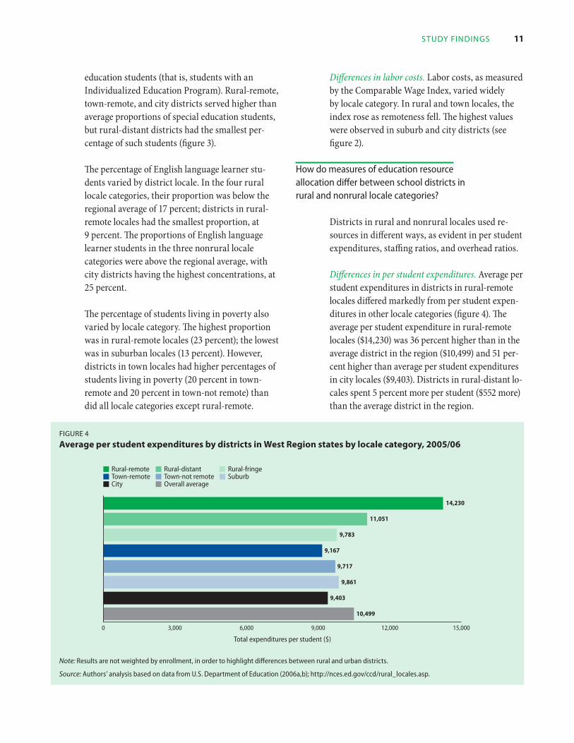
Differences in per student expenditures. Average per student expenditures in districts in rural-remote locales differed markedly from per student expen-ditures in other locale categories (figure 4). The average per student expenditure in rural-remote locales ($14,230) was 36 percent higher than in the average district in the region ($10,499) and 51 per-cent higher than average per student expenditures in city locales ($9,403). Districts in rural-distant lo-cales spent 5 percent more per student ($552 more) than the average district in the region.
0 3,000 6,000 9,000 12,000 15,000
Total expenditures per student ($)
Rural-remote Rural-distant Rural-fringeTown-remote Town-not remote SuburbCity Overall average
14,230
11,051
9,783
9,167
9,717
9,861
9,403
10,499
figure 4
Average per student expenditures by districts in West Region states by locale category, 2005/06
Note: Results are not weighted by enrollment, in order to highlight differences between rural and urban districts.
Source: Authors’ analysis based on data from U.S. Department of Education (2006a,b); http://nces.ed.gov/ccd/rural_locales.asp.

12 do SchoolS in rural and nonrural diSTricTS allocaTe reSourceS differenTly? paTTernS in The WeST region STaTeS
Districts in city, suburb, towns (not remote and remote), and rural-fringe locales all spent less than the regional average of $5,202 on instruction; per student instructional spending was above average in rural-remote ($6,704) and rural-distant ($5,582) districts (figure 5). Spending on administration and student support followed a similar pattern. Relative differences in transportation expenditures were much larger, with districts in rural-remote locales spending almost 4.5 times as much as districts in city locales.
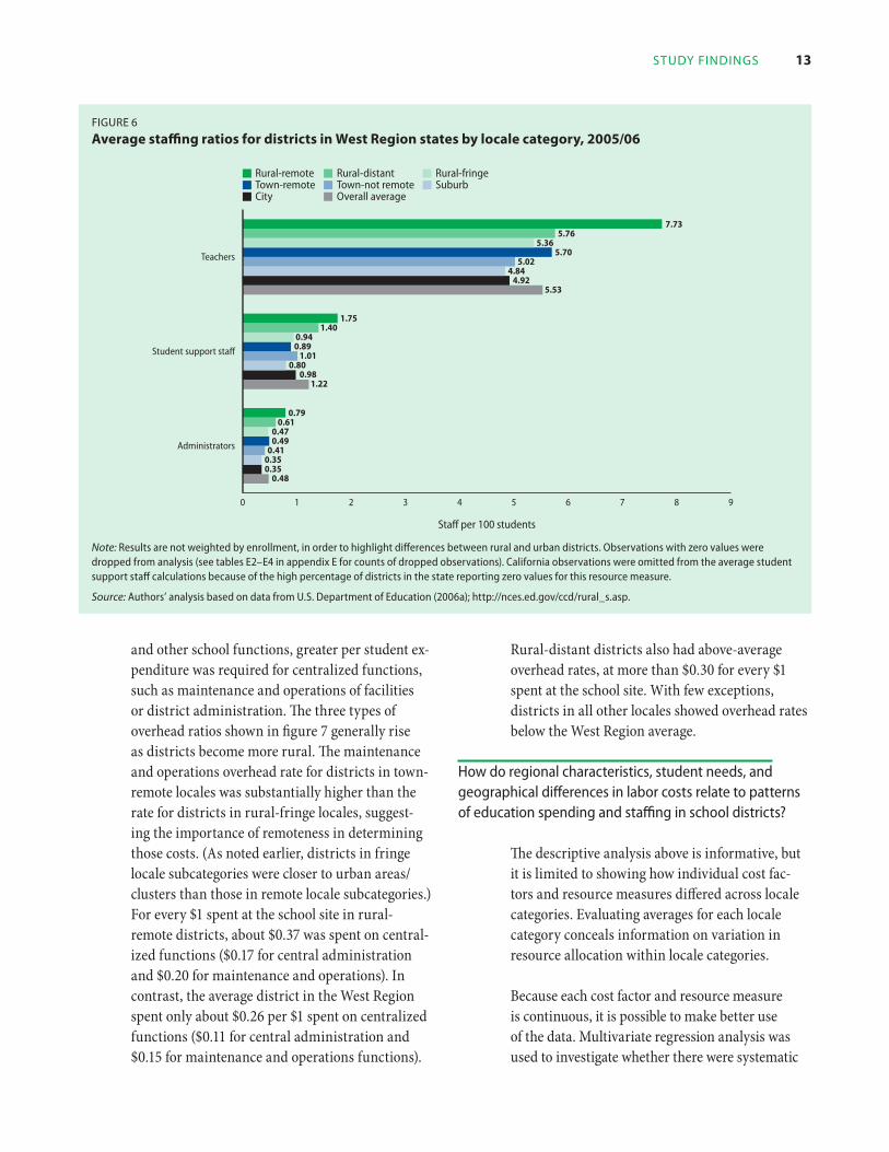
Differences in staffing ratios. Rural-remote dis-tricts employed the highest number of full-time equivalent teachers per 100 students (7.73, or about 13 students per teacher), 40 percent more than the regional average (5.53, or about 18 students per teacher; figure 6). Teacher staffing ratios in rural-distant (5.76) and rural-fringe (5.36) districts were much closer to the regional average.
Patterns for student support staff and administra-tors followed the patterns for expenditures more closely than did teacher ratios. However, for all three staff types, staffing ratios were above the overall district average in the average rural-remote and rural-distant district. Student support staff ratios were 1.75 per 100 students in rural-remote districts and 1.40 per 100 students in rural-distant districts, much higher than the West Region average of 1.22. Districts in all other locales had no more than 1.01 student support staff per 100 students. The ratio of administrators to 100 stu-dents was 0.79 in rural-remote districts and 0.61 in rural-distant districts. Ratios in all other locales except town-remote were below the West Region average of 0.48 administrators per 100 students.
Differences in overhead ratios. Diseconomies of scale in districts with low student population den-sity meant that, relative to expenditures in higher density districts, for every $1 spent on instruction
0 2,000 4,000 6,000 8,000
Total expenditures per student ($)
Rural-remote Rural-distant Rural-fringeTown-remote Town-not remote SuburbCity Overall average
Transportation
Administrationand student
support
Instruction
6,7045,582
4,9874,7244,763
4,8714,728
5,202
4,3633,189
2,5332,4732,4752,492
2,4362,846
893564
340320
263179200
378
figure 5
Average per student expenditures on instruction, administration and student support, and transportation by districts in West Region states by locale category, 2005/06
Note: Results are not weighted by enrollment, in order to highlight differences between rural and urban districts. Observations with zero values reported for transportation were dropped from analysis (see table E1 in appendix E for counts of dropped observations).
Source: Authors’ analysis based on data from U.S. Department of Education (2006a,b); http://nces.ed.gov/ccd/rural_locales.asp.
STudy findingS 13
0 1 2 3 4 5 6 7 8 9
Staff per 100 students
Rural-remote Rural-distant Rural-fringeTown-remote Town-not remote SuburbCity Overall average
Administrators
Student support staff
Teachers
7.735.76
5.365.70
5.024.84
4.925.53
1.751.40
0.940.89
1.010.80
0.981.22
0.790.61
0.470.49
0.410.350.35
0.48
figure 6
Average staffing ratios for districts in West Region states by locale category, 2005/06
Note: Results are not weighted by enrollment, in order to highlight differences between rural and urban districts. Observations with zero values were dropped from analysis (see tables E2–E4 in appendix E for counts of dropped observations). California observations were omitted from the average student support staff calculations because of the high percentage of districts in the state reporting zero values for this resource measure.
Source: Authors’ analysis based on data from U.S. Department of Education (2006a); http://nces.ed.gov/ccd/rural_s.asp.
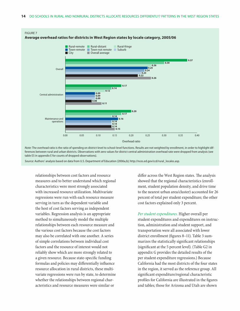
and other school functions, greater per student ex-penditure was required for centralized functions, such as maintenance and operations of facilities or district administration. The three types of overhead ratios shown in figure 7 generally rise as districts become more rural. The maintenance and operations overhead rate for districts in town-remote locales was substantially higher than the rate for districts in rural-fringe locales, suggest-ing the importance of remoteness in determining those costs. (As noted earlier, districts in fringe locale subcategories were closer to urban areas/clusters than those in remote locale subcategories.) For every $1 spent at the school site in rural-remote districts, about $0.37 was spent on central-ized functions ($0.17 for central administration and $0.20 for maintenance and operations). In contrast, the average district in the West Region spent only about $0.26 per $1 spent on centralized functions ($0.11 for central administration and $0.15 for maintenance and operations functions).
Rural-distant districts also had above-average overhead rates, at more than $0.30 for every $1 spent at the school site. With few exceptions, districts in all other locales showed overhead rates below the West Region average.
How do regional characteristics, student needs, and geographical differences in labor costs relate to patterns of education spending and staffing in school districts?
The descriptive analysis above is informative, but it is limited to showing how individual cost fac-tors and resource measures differed across locale categories. Evaluating averages for each locale category conceals information on variation in resource allocation within locale categories.
Because each cost factor and resource measure is continuous, it is possible to make better use of the data. Multivariate regression analysis was used to investigate whether there were systematic
14 Do schools in rural anD nonrural Districts allocate resources Differently? patterns in the West region states
0.00 0.05 0.10 0.15 0.20 0.25 0.30 0.35 0.40
Overhead ratio
Rural-remote Rural-distant Rural-fringeTown-remote Town-not remote SuburbCity Overall average
Maintenance andoperations
Central administration
Overall
0.370.30
0.260.25
0.240.23
0.220.26
0.170.14
0.120.090.090.09
0.080.11
0.200.17
0.140.16
0.140.140.14
0.15
figure 7
Average overhead ratios for districts in West Region states by locale category, 2005/06
Note: The overhead ratio is the ratio of spending on district-level to school-level functions. Results are not weighted by enrollment, in order to highlight dif-ferences between rural and urban districts. Observations with zero values for district central administration overhead rate were dropped from analysis (see table E5 in appendix E for counts of dropped observations).
Source: Authors’ analysis based on data from U.S. Department of Education (2006a,b); http://nces.ed.gov/ccd/rural_locales.asp.
relationships between cost factors and resource measures and to better understand which regional characteristics were most strongly associated with increased resource utilization. Multivariate regressions were run with each resource measure serving in turn as the dependent variable and the host of cost factors serving as independent variables. Regression analysis is an appropriate method to simultaneously model the multiple relationships between each resource measure and the various cost factors because the cost factors may also be correlated with one another. A series of simple correlations between individual cost factors and the resource of interest would not reliably show which are more strongly related to a given resource. Because state-specific funding formulas and policies may differentially influence resource allocation in rural districts, these multi-variate regressions were run by state, to determine whether the relationships between regional char-acteristics and resource measures were similar or
differ across the West Region states. The analysis showed that the regional characteristics (enroll-ment, student population density, and drive time to the nearest urban area/cluster) accounted for 26 percent of total per student expenditure; the other cost factors explained only 3 percent.
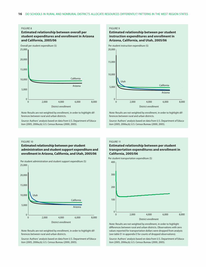
Per student expenditures. Higher overall per student expenditures and expenditures on instruc-tion, administration and student support, and transportation were all associated with lower district enrollment (figures 8–11). Table 3 sum-marizes the statistically significant relationships (significant at the 5 percent level). (Table G2 in appendix G provides the detailed results of the per student expenditure regressions.) Because California had the most districts of the four states in the region, it served as the reference group. All significant expenditure/regional characteristic profiles for California are illustrated in the figures and tables; those for Arizona and Utah are shown

STudy findingS 15
Table 3
Regression results: statistically significant relationships between regional characteristicexpenditures in california, Arizona, and utah, 2005/06
s and per student
administration and State/variable overall instruction student support Transportation
number of significant relationships
california (different from zero at the 5 percent significance level?)
enrollment yes yes yes yes 4
Student population density yes no no yes 2
drive time yes yes yes no 3
arizona (different from california at the 5 percent significance level?)
enrollment yes yes yes no 3
Student population density no no no no 0
drive time no no no no 0
utah (different from california at the 5 percent significance level?)
enrollment no yes yes no 2
Student population density no no no no 0
drive time no no no no 0
Note: Nevada was excluded from these multivariate analyses because the small number of school districts (17) in the state madestimate model parameters.
e it impossible to reliably
Source: Authors’ analysis based on data from U.S. Department of Education (2005, 2006a,b); U.S. Census Bureau (2000, 2005).
only if they differed significantly from those for California.7
The average rural-remote district in California had 296 students — less than 5 percent of the average district enrollment for the state (6,427 students). Overall per student expenditure in such a dis-trict was 8 percent higher than in a district with average enrollment for the state ($9,918 versus $9,204); expenditure on instruction was 17 percent higher ($5,563 versus $4,738); and expenditure on administration and student support was 18 per-cent higher ($8,750 versus $7,416), holding the other cost factors constant. (Appendix F details how the differential in overall per student expen-diture in this example was calculated. The other differentials were calculated in a similar fashion.) In Arizona and California, as district enrollment fell below about 1,000 students, districts began to show pronounced increases in overall per student expenditure as well as in expenditures on all spe-cific categories examined (see figures 8–11).
Per student transportation expenditures by enroll-ment in California districts showed a somewhat different pattern from that of overall, instructional, and administration and student support spend-ing per student by enrollment (see figure 11).8 Per student transportation expenditures were much higher in low-enrollment school districts than in districts with larger enrollments. However, above a threshold of 750 students, transportation expenditures rose with increasing enrollments. For example, according to the regression analysis, an average very small California school district of 50 students spent an estimated $163 per student on transportation, an average rural-remote school district of 296 students spent $127 per student, and an average-size West Region district of 6,427 students spent $147 per student. Higher per student expenditures on transportation in rural districts could reflect the fact that the students lived farther from one another and from their school or that the district provided transportation to a higher propor-tion of its students — or both.
16 do SchoolS in rural and nonrural diSTricTS allocaTe reSourceS differenTly? paTTernS in The WeST region STaTeS
0 2,000 4,000 6,000 8,0000
5,000
10,000
15,000
20,000
25,000Overall per student expenditure ($)
California
District enrollment
Arizona
figure 8
estimated relationship between overall per student expenditures and enrollment in Arizona and california, 2005/06
Note: Results are not weighted by enrollment, in order to highlight dif-ferences between rural and urban districts.
Source: Authors’ analysis based on data from U.S. Department of Educa-tion (2005, 2006a,b); U.S. Census Bureau (2000, 2005).
0 2,000 4,000 6,000 8,0000
5,000
10,000
15,000
20,000Per student instruction expenditure ($)
Utah
District enrollment
Arizona
California
figure 9
estimated relationship between per student instruction expenditures and enrollment in Arizona, california, and utah, 2005/06
Note: Results are not weighted by enrollment, in order to highlight dif-ferences between rural and urban districts.
Source: Authors’ analysis based on data from U.S. Department of Educa-tion (2005, 2006a,b); U.S. Census Bureau (2000, 2005).
0 2,000 4,000 6,000 8,0000
5,000
10,000
15,000
20,000
25,000Per student administration and student support expenditure ($)
Utah
District enrollment
Arizona
California
figure 10
estimated relationship between per student administration and student support expenditure and enrollment in Arizona, california, and utah, 2005/06
Note: Results are not weighted by enrollment, in order to highlight dif-ferences between rural and urban districts.
Source: Authors’ analysis based on data from U.S. Department of Educa-tion (2005, 2006a,b); U.S. Census Bureau (2000, 2005).
0
100
200
300
400Per student transportation expenditure ($)
District enrollment
0 2,000 4,000 6,000 8,000
figure 11
estimated relationship between per student transportation expenditures and enrollment in california, 2005/06
Note: Results are not weighted by enrollment, in order to highlight differences between rural and urban districts. Observations with zero values reported for transportation dollars were dropped from analysis (see table E1 in appendix E for counts of dropped observations).
Source: Authors’ analysis based on data from U.S. Department of Educa-tion (2005, 2006a,b); U.S. Census Bureau (2000, 2005).
STudy findingS 17
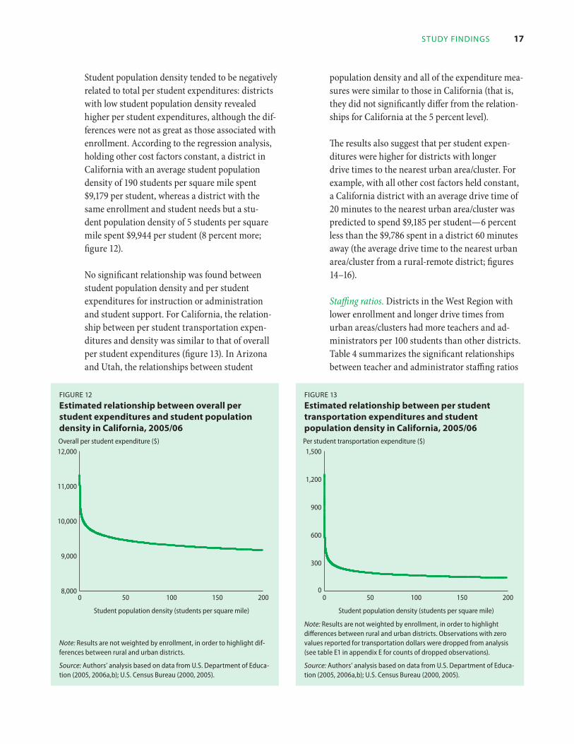
Student population density tended to be negatively related to total per student expenditures: districts with low student population density revealed higher per student expenditures, although the dif-ferences were not as great as those associated with enrollment. According to the regression analysis, holding other cost factors constant, a district in California with an average student population density of 190 students per square mile spent $9,179 per student, whereas a district with the same enrollment and student needs but a stu-dent population density of 5 students per square mile spent $9,944 per student (8 percent more; figure 12).
No significant relationship was found between student population density and per student expenditures for instruction or administration and student support. For California, the relation-ship between per student transportation expen-ditures and density was similar to that of overall per student expenditures (figure 13). In Arizona and Utah, the relationships between student
population density and all of the expenditure mea-sures were similar to those in California (that is, they did not significantly differ from the relation-ships for California at the 5 percent level).
The results also suggest that per student expen-ditures were higher for districts with longer drive times to the nearest urban area/cluster. For example, with all other cost factors held constant, a California district with an average drive time of 20 minutes to the nearest urban area/cluster was predicted to spend $9,185 per student —6 p ercent less than the $9,786 spent in a district 60 minutes away (the average drive time to the nearest urban area/cluster from a rural-remote district; figures 14–16).
Staffing ratios. Districts in the West Region with lower enrollment and longer drive times from urban areas/clusters had more teachers and ad-ministrators per 100 students than other districts. Table 4 summarizes the significant relationships between teacher and administrator staffing ratios
0 50 100 150 2008,000
9,000
10,000
11,000
12,000Overall per student expenditure ($)
Student population density (students per square mile)
figure 12
estimated relationship between overall per student expenditures and student population density in california, 2005/06
Note: Results are not weighted by enrollment, in order to highlight dif-ferences between rural and urban districts.
Source: Authors’ analysis based on data from U.S. Department of Educa-tion (2005, 2006a,b); U.S. Census Bureau (2000, 2005).
0 50 100 150 2000
300
600
900
1,200
1,500Per student transportation expenditure ($)
Student population density (students per square mile)
figure 13
estimated relationship between per student transportation expenditures and student population density in california, 2005/06
Note: Results are not weighted by enrollment, in order to highlight differences between rural and urban districts. Observations with zero values reported for transportation dollars were dropped from analysis (see table E1 in appendix E for counts of dropped observations).
Source: Authors’ analysis based on data from U.S. Department of Educa-tion (2005, 2006a,b); U.S. Census Bureau (2000, 2005).

18 do SchoolS in rural and nonrural diSTricTS allocaTe reSourceS differenTly? paTTernS in The WeST region STaTeS
0 15 30 45 60 758,750
9,000
9,250
9,500
9,750
10,000Overall per student expenditure ($)
Drive time to nearest urban area/cluster (minutes)
figure 14
estimated relationship between overall per student expenditure and drive time to nearest urban area/cluster in california, 2005/06
Note: Results are not weighted by enrollment, in order to highlight dif-ferences between rural and urban districts.
Source: Authors’ analysis based on data from U.S. Department of Educa-tion (2005, 2006a,b); U.S. Census Bureau (2000, 2005).
0 15 30 45 60 754,600
4,700
4,800
4,900
5,000Per student instruction expenditure ($)
Drive time to nearest urban area/cluster (minutes)
figure 15
estimated relationship between per student instruction expenditures and drive time to nearest urban area/cluster in california, 2005/06
Note: Results are not weighted by enrollment, in order to highlight dif-ferences between rural and urban districts.
Source: Authors’ analysis based on data from U.S. Department of Educa-tion (2005, 2006a,b); U.S. Census Bureau (2000, 2005).
0 15 30 45 60 757,000
7,250
7,500
7,750
8,000Per student administration and student support expenditure ($)
Drive time to nearest urban area/cluster (minutes)
figure 16
estimated relationship between per student administration and student support expenditure and drive time to nearest urban area/cluster in california, 2005/06
Note: Results are not weighted by enrollment, in order to highlight dif-ferences between rural and urban districts.
Source: Authors’ analysis based on data from U.S. Department of Educa-tion (2005, 2006a,b); U.S. Census Bureau (2000, 2005).
and regional characteristics in each state. (De-tailed results of the regressions of the staffing ratio resource measures can be found in table G3 in appendix G.)
Like per student expenditures, teacher and ad-ministrator staffing ratios varied significantly with enrollment (figures 17 and 18). In Arizona, Cali-fornia, and Utah, the number of teachers per 100 students was substantially higher for districts with fewer than about 400 students. For example, an Arizona district of 200 students was expected to employ 6.3 teachers per 100 students, whereas an average-size district (of 4,560 students) in the state was predicted to have a teacher staffing ratio of 4.9 teachers per 100 students. (Appendix F details how this differential was calculated.)
Administrator staffing ratios in California and Arizona showed similar patterns (see figure 18). In Arizona, the average-size district of 4,560 students was predicted to have 0.28 administrators per 100 students, whereas a district of 200 students was predicted to have 0.73. This relationship in

STudy findingS 19
Table 4
Regression results: statistically significant relationships between regional characteristics and staffing ratios in california, Arizona, and utah, 2005/06
Teachers administrators number of significant State/variable per 100 students per 100 students relationships
california (different from zero at the 5 percent significance level?)
enrollment yes yes 2
Student population density no yes 1
drive time yes yes 2
arizona (different from california at the 5 percent significance level?)
enrollment yes yes 2
Student population density no no 0
drive time no no 0
utah (different from california at the 5 percent significance level?)
enrollment yes yes 2
Student population density no no 0
drive time no no 0
Note: Nevada was excluded from these multivariate analyses because the small number of school districts (17) in the state made it impossible to reliably estimate model parameters.
Source: Authors’ analysis based on data from U.S. Department of Education (2005, 2006a,b); U.S. Census Bureau (2000, 2005).
0 2,000 4,000 6,000 8,0000
2
4
6
8
10Teachers per 100 students (full-time equivalent)
Utah
District enrollment
Arizona
California
figure 17
estimated relationship between teacher staffing ratio and enrollment in Arizona, california, and utah, 2005/06
Note: Results are not weighted by enrollment, in order to highlight differences between rural and urban districts. Observations with zero values reported for teacher staffing ratio were dropped from analysis (see table E2 in appendix E for counts of dropped observations).
Source: Authors’ analysis based on data from U.S. Department of Educa-tion (2005, 2006a,b); U.S. Census Bureau (2000, 2005).
0 2,000 4,000 6,000 8,0000.0
0.5
1.0
1.5
2.0Administrators per 100 students (full-time equivalent)
Utah
District enrollment
Arizona
California
figure 18
estimated relationship between administrator staffing ratio and enrollment in Arizona, california, and utah, 2005/06
Note: Results are not weighted by enrollment, in order to highlight dif-ferences between rural and urban districts. Observations with zero val-ues reported for administrator staffing ratio were dropped from analysis (see table E4 in appendix E for counts of dropped observations).
Source: Authors’ analysis based on data from U.S. Department of Educa-tion (2005, 2006a,b); U.S. Census Bureau (2000, 2005).

20 do SchoolS in rural and nonrural diSTricTS allocaTe reSourceS differenTly? paTTernS in The WeST region STaTeS
Arizona and Utah was statistically significantly different from that in California. Utah in particu-lar showed a more gradual increase in administra-tor staffing levels with decreasing enrollments.
Analysis of administrator staffing ratios found this resource measure to be significantly related to stu-dent population density in California (figure 19). Teacher and administrator staffing ratios were also related to drive time to the nearest urban area/cluster (figures 20 and 21); statistically significant differences were not evident across states.
District overhead. The overhead ratio of district- to school-level expenditures was higher in smaller districts with less dense student populations and located farther from urban areas/clusters. (Table G3 in appendix G provides the detailed results of the overhead ratio regressions.) As the estimated relationships between the regional characteris-tics and each of the three overhead rates (overall, central administration, and maintenance and operations) showed similar patterns, presentation
0 50 100 150 2000.30
0.35
0.40
0.45Administrators per 100 students (full-time equivalent)
Student population density (students per square mile)
figure 19
estimated relationship between administrator staffing ratio and student population density in california, 2005/06
Note: Results are not weighted by enrollment, in order to highlight dif-ferences between rural and urban districts. Observations with zero val-ues reported for administrator staffing ratio were dropped from analysis (see table E4 in appendix E for counts of dropped observations).
Source: Authors’ analysis based on data from U.S. Department of Educa-tion (2005, 2006a,b); U.S. Census Bureau (2000, 2005).
0 15 30 45 60 754.6
4.7
4.8
4.9
5.0Teachers per 100 students (full-time equivalent)
Drive time to nearest urban area/cluster (minutes)
figure 20
estimated relationship between teacher staffing ratio and drive time to nearest urban area/cluster in california, 2005/06
Note: Results are not weighted by enrollment, in order to highlight differences between rural and urban districts. Observations with zero values reported for teacher staffing ratio were dropped from the analy-sis (see table E2 in appendix E for counts of dropped observations).
Source: Authors’ analysis based on data from U.S. Department of Educa-tion (2005, 2006a,b); U.S. Census Bureau (2000, 2005).
0 15 30 45 60 750.30
0.32
0.34
0.36Administrators per 100 students (full-time equivalent)
Drive time to nearest urban area/cluster (minutes)
figure 21
estimated relationship between administrator staffing ratio and drive time to nearest urban area/cluster in california, 2005/06
Note: Results are not weighted by enrollment, in order to highlight differences between rural and urban districts. Observations with zero values reported for administrator staffing ratio were dropped from the analysis (see table E4 in appendix E for counts of dropped observations).
Source: Authors’ analysis based on data from U.S. Department of Educa-tion (2005, 2006a,b); U.S. Census Bureau (2000, 2005).
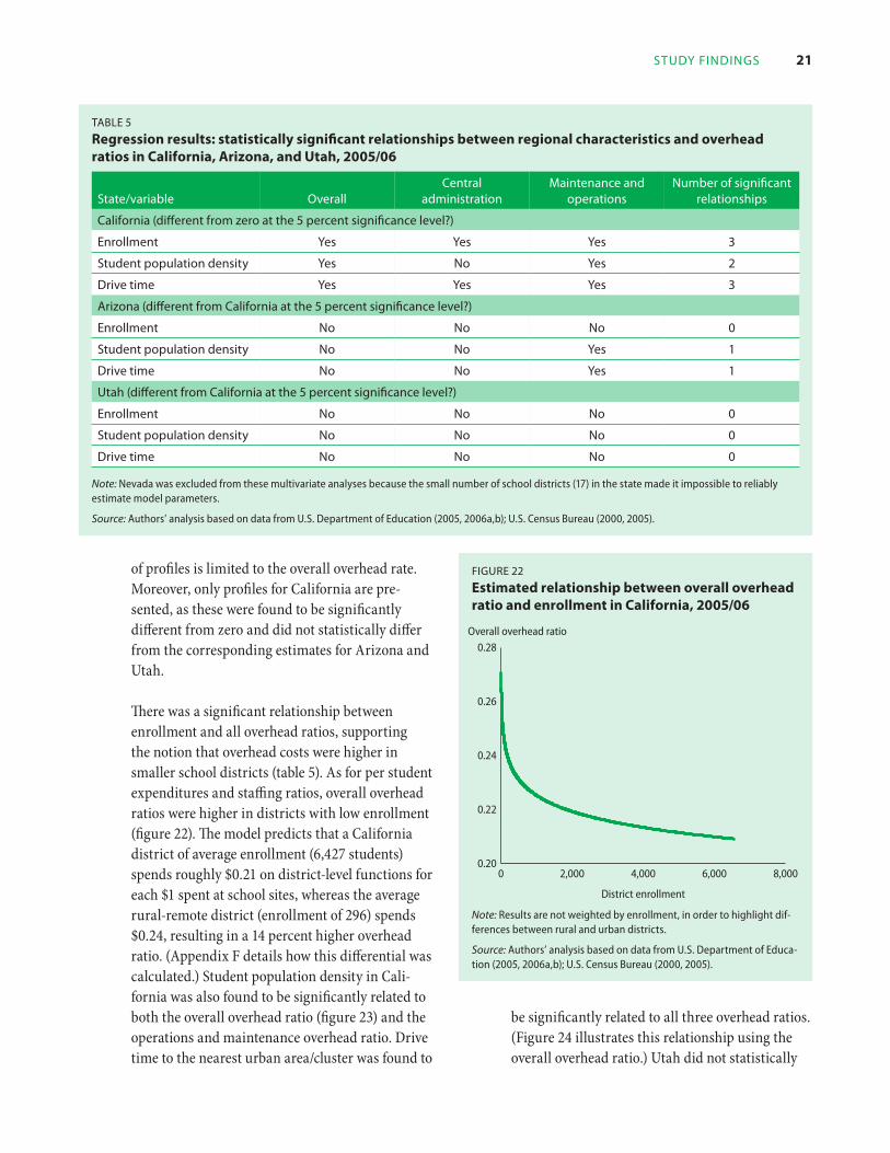
STudy findingS 21
Table 5
Regression results: statistically significant relationships between regional characteristicratios in california, Arizona, and utah, 2005/06
s and overhead
central maintenance and State/variable overall administration operations
number of significant relationships
california (different from zero at the 5 percent significance level?)
enrollment yes yes yes 3
Student population density yes no yes 2
drive time yes yes yes 3
arizona (different from california at the 5 percent significance level?)
enrollment no no no 0
Student population density no no yes 1
drive time no no yes 1
utah (different from california at the 5 percent significance level?)
enrollment no no no 0
Student population density no no no 0
drive time no no no 0
Note: Nevada was excluded from these multivariate analyses because the small number of school districts (17) in the state madestimate model parameters.
e it impossible to reliably
Source: Authors’ analysis based on data from U.S. Department of Education (2005, 2006a,b); U.S. Census Bureau (2000, 2005).
0 2,000 4,000 6,000 8,0000.20
0.22
0.24
0.26
0.28Overall overhead ratio
District enrollment
figure 22
estimated relationship between overall overhead ratio and enrollment in california, 2005/06
Note: Results are not weighted by enrollment, in order to highlight dif-ferences between rural and urban districts.
Source: Authors’ analysis based on data from U.S. Department of Educa-tion (2005, 2006a,b); U.S. Census Bureau (2000, 2005).
of profiles is limited to the overall overhead rate. Moreover, only profiles for California are pre-sented, as these were found to be significantly different from zero and did not statistically differ from the corresponding estimates for Arizona and Utah.
There was a significant relationship between enrollment and all overhead ratios, supporting the notion that overhead costs were higher in smaller school districts (table 5). As for per student expenditures and staffing ratios, overall overhead ratios were higher in districts with low enrollment (figure 22). The model predicts that a California district of average enrollment (6,427 students) spends roughly $0.21 on district-level functions for each $1 spent at school sites, whereas the average rural-remote district (enrollment of 296) spends $0.24, resulting in a 14 percent higher overhead ratio. (Appendix F details how this differential was calculated.) Student population density in Cali-fornia was also found to be significantly related to both the overall overhead ratio (figure 23) and the operations and maintenance overhead ratio. Drive time to the nearest urban area/cluster was found to
be significantly related to all three overhead ratios. (Figure 24 illustrates this relationship using the overall overhead ratio.) Utah did not statistically

22 do SchoolS in rural and nonrural diSTricTS allocaTe reSourceS differenTly? paTTernS in The WeST region STaTeS
0 50 100 150 2000.20
0.22
0.24
0.26
0.28
0.30Overall overhead ratio
Student population density (students per square mile)
figure 23
estimated relationship between overall overhead ratio and student population density in california, 2005/06
Note: Results are not weighted by enrollment, in order to highlight dif-ferences between rural and urban districts.
Source: Authors’ analysis based on data from U.S. Department of Educa-tion (2005, 2006a,b); U.S. Census Bureau (2000, 2005).
0 15 30 45 60 750.20
0.21
0.22
0.23Overall overhead ratio
Drive time to nearest urban area/cluster (minutes)
figure 24
estimated relationship between overall overhead ratio and drive time to nearest urban area/cluster in california, 2005/06
Note: Results are not weighted by enrollment, in order to highlight dif-ferences between rural and urban districts.
Source: Authors’ analysis based on data from U.S. Department of Educa-tion (2005, 2006a,b); U.S. Census Bureau (2000, 2005).
differ from California in the relationship between any of the overhead ratios and regional charac-teristics. Only in Arizona was the relationship between student population density and the main-tenance and operations overhead ratio statistically different from that in California.
sTuDy limiTATions
There are several limitations to the analysis in this report. First, the results are descriptive; they show how per student expenditures, staffing ratios, and overhead ratios vary across regional characteris-tics, student needs, and geographic differences in labor costs. Because student achievement, gradua-tion rates, and other outcomes were not considered, nothing can be said about the cost of achieving a particular level of student outcome or how such outcomes may differ in rural and nonrural dis-tricts. As such, the findings cannot be interpreted as illustrating the differential costs of producing a given set of education outcomes between or within groups of rural and nonrural school districts.
Second, this analysis did not model the mecha-nisms that underlie all the resource allocation decisions made by districts. Doing so would require a system that incorporates not only the relationships between cost factors and resource measures but also the availability of funding through various revenue streams and community demand for education quality (levels of education outcome). The estimated relationships should not be interpreted as causal. The analysis here was exploratory and correlational — it simply observed districts’ resource allocation decisions in order to understand how the decisions varied with regional characteristics, student needs, and geographic dif-ferences in labor costs.
Third, districts that reported implausible zero values for various resource measures were omitted from both the descriptive and regression analyses, possibly introducing some upward bias in the calculation of average resource utilization. How-ever, in only two cases did the number of dropped records exceed 5 percent of the sample of districts within a state (for California transportation
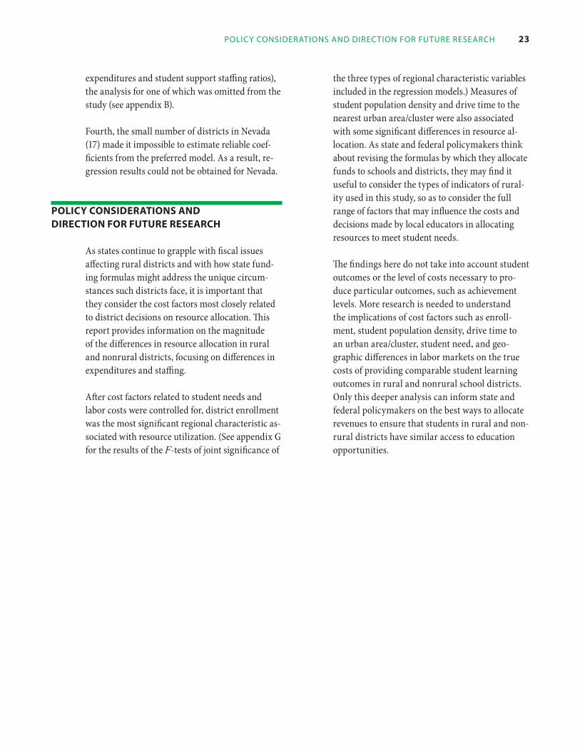
policy conSideraTionS and direcTion for fuTure reSearch 23
expenditures and student support staffing ratios), the analysis for one of which was omitted from the study (see appendix B).
Fourth, the small number of districts in Nevada (17) made it impossible to estimate reliable coef-ficients from the preferred model. As a result, re-gression results could not be obtained for Nevada.
Policy consiDeRATions AnD DiRecTion foR fuTuRe ReseARch
As states continue to grapple with fiscal issues affecting rural districts and with how state fund-ing formulas might address the unique circum-stances such districts face, it is important that they consider the cost factors most closely related to district decisions on resource allocation. This report provides information on the magnitude of the differences in resource allocation in rural and nonrural districts, focusing on differences in expenditures and staffing.
After cost factors related to student needs and labor costs were controlled for, district enrollment was the most significant regional characteristic as-sociated with resource utilization. (See appendix G for the results of the F-tests of joint significance of
the three types of regional characteristic variables included in the regression models.) Measures of student population density and drive time to the nearest urban area/cluster were also associated with some significant differences in resource al-location. As state and federal policymakers think about revising the formulas by which they allocate funds to schools and districts, they may find it useful to consider the types of indicators of rural-ity used in this study, so as to consider the full range of factors that may influence the costs and decisions made by local educators in allocating resources to meet student needs.
The findings here do not take into account student outcomes or the level of costs necessary to pro-duce particular outcomes, such as achievement levels. More research is needed to understand the implications of cost factors such as enroll-ment, student population density, drive time to an urban area/cluster, student need, and geo-graphic differences in labor markets on the true costs of providing comparable student learning outcomes in rural and nonrural school districts. Only this deeper analysis can inform state and federal policymakers on the best ways to allocate revenues to ensure that students in rural and non-rural districts have similar access to education opportunities.

24 do SchoolS in rural and nonrural diSTricTS allocaTe reSourceS differenTly? paTTernS in The WeST region STaTeS
APPenDix A DisTRibuTion of school DisTRicTs AnD sTuDenTs in WesT Region sTATes by locAle cATegoRy, 2005/06
Table A1 shows the count of districts in each locale, along with the percentage of districts in
each state that are classified in each locale category and the percentages of districts in each locale that are located in each of the four states in the West Region. Table A2 shows the same information for counts and percentages of students in each locale category. Table A2 is thus a student-weighted ver-sion of table A1.
Table a1
Distribution of school districts in West Region states by locale category, 2005/06
State/distribution Town- Town- rural- rural-measure city Suburb not remote remote fringe distant
rural-remote
Total count
arizona
count 32 17 13 23 26 34
row (percent) 15 8 6 11 13 16
column (percent) 18 6 9 33 15 18
62
30
38
207
california
count 141 273 126 34 144 150
row (percent) 15 29 13 4 15 16
column (percent) 78 92 86 49 83 81
86
9
52
954
nevada
count 2 1 2 5 2 1
row (percent) 12 6 12 29 12 6
column (percent) 1 0 1 7 1 1
4
24
2
17
utah
count 5 7 5 8 1 1
row (percent) 13 18 13 20 3 3
column (percent) 3 2 3 11 1 1
Total count 180 298 146 70 173 186
Note: Percentages may not sum to 100 because of rounding.
13
33
8
165
40
1,218
Source: Authors’ analysis based on data from U.S. Department of Education (2006a); http://nces.ed.gov/ccd/rural_locales.asp.
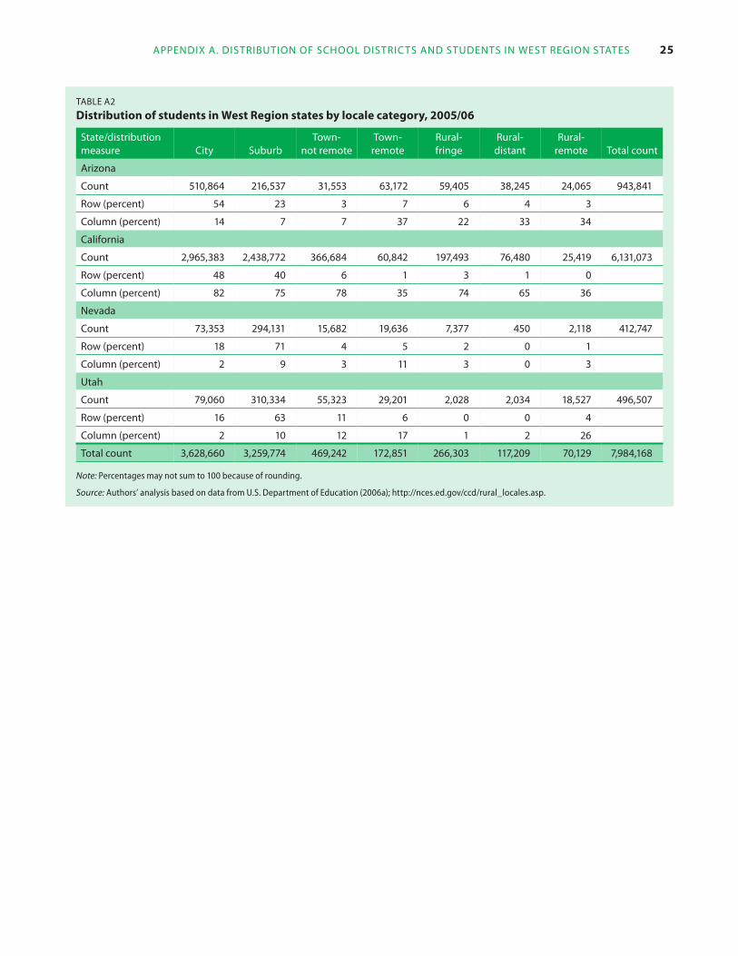
appendix a. diSTribuTion of School diSTricTS and STudenTS in WeST region STaTeS 25
Table a2
Distribution of students in West Region states by locale category, 2005/06
State/distribution Town- Town- rural- rural-measure city Suburb not remote remote fringe distant
rural-remote Total count
arizona
count 510,864 216,537 31,553 63,172 59,405 38,245
row (percent) 54 23 3 7 6 4
column (percent) 14 7 7 37 22 33
24,065
3
34
943,841
california
count 2,965,383 2,438,772 366,684 60,842 197,493 76,480
row (percent) 48 40 6 1 3 1
column (percent) 82 75 78 35 74 65
25,419
0
36
6,131,073
nevada
count 73,353 294,131 15,682 19,636 7,377 450
row (percent) 18 71 4 5 2 0
column (percent) 2 9 3 11 3 0
2,118
1
3
412,747
utah
count 79,060 310,334 55,323 29,201 2,028 2,034
row (percent) 16 63 11 6 0 0
column (percent) 2 10 12 17 1 2
Total count 3,628,660 3,259,774 469,242 172,851 266,303 117,209
Note: Percentages may not sum to 100 because of rounding.
18,527
4
26
70,129
496,507
7,984,168
Source: Authors’ analysis based on data from U.S. Department of Education (2006a); http://nces.ed.gov/ccd/rural_locales.asp.
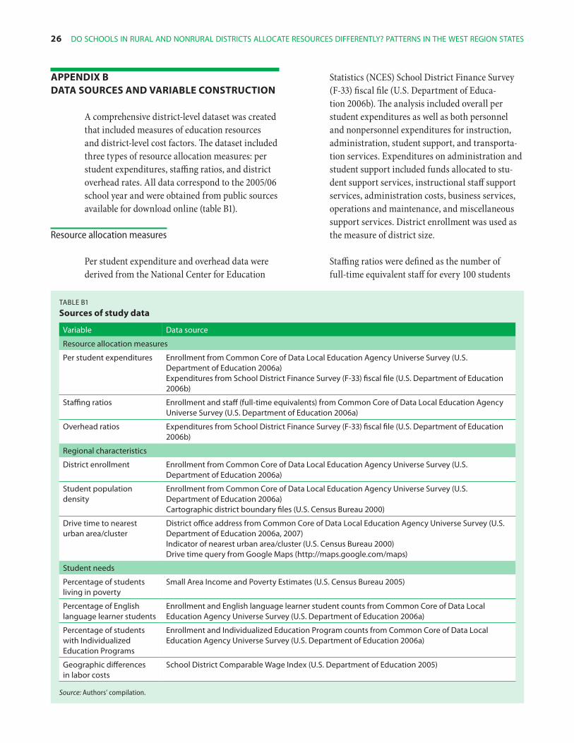
26 do SchoolS in rural and nonrural diSTricTS allocaTe reSourceS differenTly? paTTernS in The WeST region STaTeS
APPenDix b DATA souRces AnD vARiAble consTRucTion
A comprehensive district-level dataset was created that included measures of education resources and district-level cost factors. The dataset included three types of resource allocation measures: per student expenditures, staffing ratios, and district overhead rates. All data correspond to the 2005/06 school year and were obtained from public sources available for download online (table B1).
Resource allocation measures
Per student expenditure and overhead data were derived from the National Center for Education
Statistics (NCES) School District Finance Survey (F-33) fiscal file (U.S. Department of Educa-tion 2006b). The analysis included overall per student expenditures as well as both personnel and nonpersonnel expenditures for instruction, administration, student support, and transporta-tion services. Expenditures on administration and student support included funds allocated to stu-dent support services, instructional staff support services, administration costs, business services, operations and maintenance, and miscellaneous support services. District enrollment was used as the measure of district size.
Staffing ratios were defined as the number of full-time equivalent staff for every 100 students
Table b1
sources of study data
Variable data source
resource allocation measures
per student expenditures enrollment from common core of data local education agency universe Survey (u.S. department of education 2006a)expenditures from School district finance Survey (f-33) fiscal file (u.S. department of education 2006b)
Staffing ratios enrollment and staff (full-time equivalents) from common core of data local education agency universe Survey (u.S. department of education 2006a)
overhead ratios expenditures from School district finance Survey (f-33) fiscal file (u.S. department of education 2006b)
regional characteristics
district enrollment enrollment from common core of data local education agency universe Survey (u.S. department of education 2006a)
Student population enrollment from common core of data local education agency universe Survey (u.S. density department of education 2006a)
cartographic district boundary files (u.S. census bureau 2000)
drive time to nearest district office address from common core of data local education agency universe Survey (u.S. urban area/cluster department of education 2006a, 2007)
indicator of nearest urban area/cluster (u.S. census bureau 2000)drive time query from google maps (http://maps.google.com/maps)
Student needs
percentage of students Small area income and poverty estimates (u.S. census bureau 2005)living in poverty
percentage of english enrollment and english language learner student counts from common core of data local language learner students education agency universe Survey (u.S. department of education 2006a)
percentage of students enrollment and individualized education program counts from common core of data local with individualized education agency universe Survey (u.S. department of education 2006a)education programs
geographic differences School district comparable Wage index (u.S. department of education 2005)in labor costs
Source: Authors’ compilation.
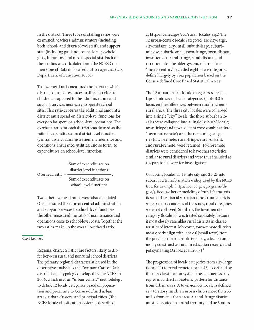
appendix b. daTa SourceS and Variable conSTrucTion 27
in the district. Three types of staffing ratios were examined: teachers, administrators (including both school- and district-level staff), and support staff (including guidance counselors, psycholo-gists, librarians, and media specialists). Each of these ratios was calculated from the NCES Com-mon Core of Data on local education agencies (U.S. Department of Education 2006a).
The overhead ratio measured the extent to which districts devoted resources to direct services to children as opposed to the administration and support services necessary to operate school sites. This ratio captures the additional amount a district must spend on district-level functions for every dollar spent on school-level operations. The overhead ratio for each district was defined as the ratio of expenditures on district-level functions (central district administration, maintenance and operations, insurance, utilities, and so forth) to expenditures on school-level functions:
Sum of expenditures on district-level functionsOverhead ratio = . Sum of expenditures on school-level functions
Two other overhead ratios were also calculated. One measured the ratio of central administration and support services to school-level functions; the other measured the ratio of maintenance and operations costs to school-level costs. Together the two ratios make up the overall overhead ratio.
Cost factors
Regional characteristics are factors likely to dif-fer between rural and nonrural school districts. The primary regional characteristic used in the descriptive analysis is the Common Core of Data district locale typology developed by the NCES in 2006, which uses an “urban-centric” methodology to define 12 locale categories based on popula-tion and proximity to Census-defined urban areas, urban clusters, and principal cities. (The NCES locale classification system is described
at http://nces.ed.gov/ccd/rural_locales.asp.) The 12 urban-centric locale categories are city-large, city-midsize, city-small, suburb-large, suburb-midsize, suburb-small, town-fringe, town-distant, town-remote, rural-fringe, rural-distant, and rural-remote. The older system, referred to as “metro-centric,” included eight locale categories defined largely by area population based on the Census-defined Core Based Statistical Areas.
The 12 urban-centric locale categories were col-lapsed into seven locale categories (table B2) to focus on the differences between rural and non-rural areas. The three city locales were collapsed into a single “city” locale; the three suburban lo-cales were collapsed into a single “suburb” locale; town-fringe and town-distant were combined into “town-not remote”; and the remaining catego-ries (town-remote, rural-fringe, rural-distant, and rural- remote) were retained. Town-remote districts were considered to have characteristics similar to rural districts and were thus included as a separate category for investigation.
Collapsing locales 11–13 into city and 21–23 into suburb is a transformation widely used by the NCES (see, for example, http://nces.ed.gov/programs/di-gest/). Because better modeling of rural characteris-tics and detection of variation across rural districts were primary concerns of the study, rural categories were not collapsed. Similarly, the town-remote category (locale 33) was treated separately, because it most closely resembles rural districts in charac-teristics of interest. Moreover, town-remote districts most closely align with locale 6 (small town) from the previous metro-centric typology, a locale com-monly construed as rural in education research and policymaking (Arnold et al. 2007).9
The progression of locale categories from city-large (locale 11) to rural-remote (locale 43) as defined by the new classification system does not necessarily represent a strict monotonic pattern for distance from urban areas. A town-remote locale is defined as a territory inside an urban cluster more than 35 miles from an urban area. A rural-fringe district must be located in a rural territory and be 5 miles
28 do SchoolS in rural and nonrural diSTricTS allocaTe reSourceS differenTly? paTTernS in The WeST region STaTeS
or less from an urbanized area or 2.5 miles or less from an urbanized cluster.
Study datasets contained zero values for several resource measures (per student transporta-tion expenditures; teacher, student support, and administrator staff ratios; and central administra-tion overhead expenditures). These zero values were set to missing to avoid biasing the results downward. Dropping these observations had the potential to bias the calculated resource use aver-ages and results of the regression analysis. The numbers of districts omitted from the analyses were small. In only two cases (both for Califor-nia) did the percentage of districts in a state that reported zero values for a given resource measure exceed 5 percent. In the first case, 6 percent of the districts in California reported zero transportation expenditures. The second case was much higher: 24 percent of the California districts reported zero student support staff, which called into question the validity of this measure for the state. (The ta-bles in appendix E contain the counts and percent-ages of districts— and their corresponding student populations —d ropped because of reported zero values.) Hence, all California records were omitted from the descriptive analysis of student support
staff. After the reported zero values were cleaned from the data, averages of each cost factor and resource measure for districts in each of the ag-gregated locale categories were calculated.10
Locale category was a simple way to group districts. Other characteristics more precisely described specific dimensions of rurality and remoteness. Enrollment, student population density, and average drive time to the nearest urban area/cluster provided important contex-tual information on resource allocation in rural and nonrural districts. These cost factors convey information about economies of scale, may affect the location and size of schools, are likely to play a role in decisions on student transportation, and may be associated with the availability of services for students with special needs. Regional char-acteristics therefore were variables of primary importance.
The regional characteristics variables were obtained directly or constructed from other data sources. Calculating student density required both enrollment data (U.S. Department of Education 2006a) and the area of the school district. Car-tographic files from the U.S. Census Bureau that
Table b2
Aggregation of national center for education statistics locale codes for use in this study
This study
nceS locale category aggregated locale category rural/nonrural distinction
city-large (locale 11)
city
nonrural
city-midsize (locale 12)
city-small (locale 13)
Suburb-large (locale 21)
Suburb-midsize (locale 22) Suburb
Suburb-small (locale 23)
Town-fringe (locale 31)Town-not remote
Town-distant (locale 32)
Town-remote (locale 33) Town-remote
ruralrural-fringe (locale 41) rural-fringe
rural-distant (locale 42) rural-distant
rural-remote (locale 43) rural-remote
Source: Authors’ analysis based on http://nces.ed.gov/ccd/rural_locales.asp.
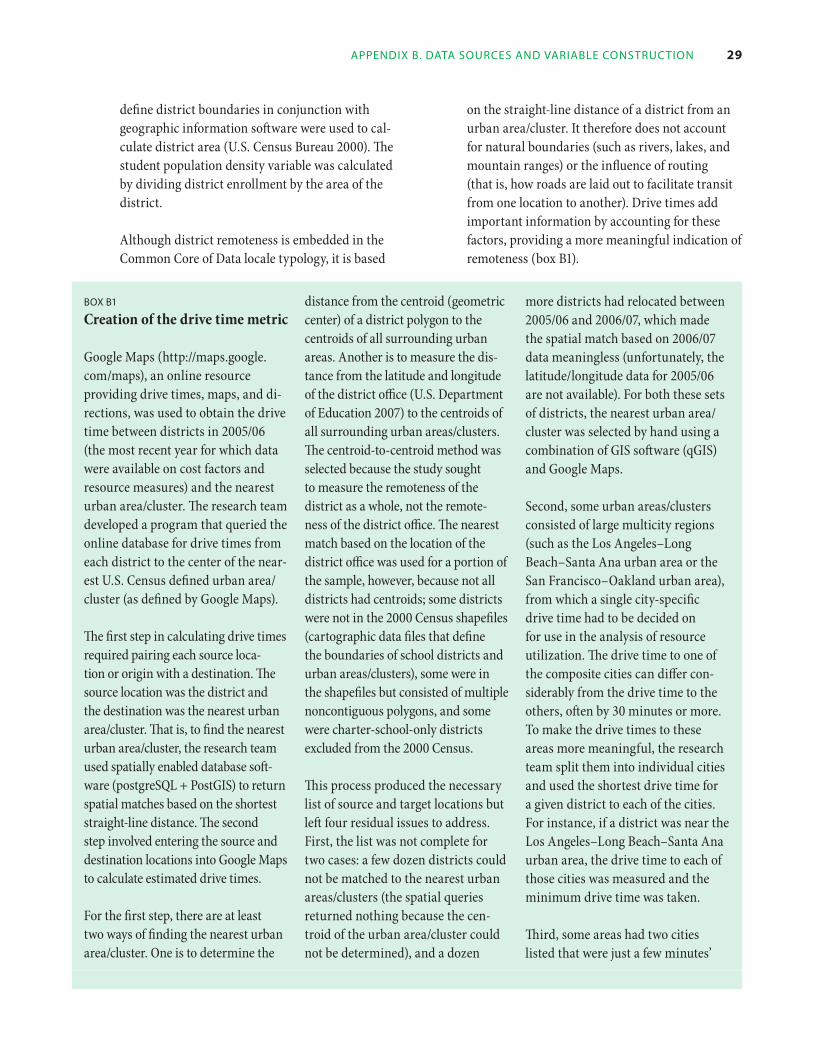
appendix b. daTa SourceS and Variable conSTrucTion 29
define district boundaries in conjunction with geographic information software were used to cal-culate district area (U.S. Census Bureau 2000). The student population density variable was calculated by dividing district enrollment by the area of the district.
Although district remoteness is embedded in the Common Core of Data locale typology, it is based
on the straight-line distance of a district from an urban area/cluster. It therefore does not account for natural boundaries (such as rivers, lakes, and mountain ranges) or the influence of routing (that is, how roads are laid out to facilitate transit from one location to another). Drive times add important information by accounting for these factors, providing a more meaningful indication of remoteness (box B1).
box b1
Creation of the drive time metric
Google Maps (http://maps.google.com/maps), an online resource providing drive times, maps, and di-rections, was used to obtain the drive time between districts in 2005/06 (the most recent year for which data were available on cost factors and resource measures) and the nearest urban area/cluster. The research team developed a program that queried the online database for drive times from each district to the center of the near-est U.S. Census defined urban area/cluster (as defined by Google Maps).
The first step in calculating drive times required pairing each source loca-tion or origin with a destination. The source location was the district and the destination was the nearest urban area/cluster. That is, to find the nearest urban area/cluster, the research team used spatially enabled database soft-ware (postgreSQL + PostGIS) to return spatial matches based on the shortest straight-line distance. The second step involved entering the source and destination locations into Google Maps to calculate estimated drive times.
For the first step, there are at least two ways of finding the nearest urban area/cluster. One is to determine the
distance from the centroid (geometric center) of a district polygon to the centroids of all surrounding urban areas. Another is to measure the dis-tance from the latitude and longitude of the district office (U.S. Department of Education 2007) to the centroids of all surrounding urban areas/clusters. The centroid-to-centroid method was selected because the study sought to measure the remoteness of the district as a whole, not the remote-ness of the district office. The nearest match based on the location of the district office was used for a portion of the sample, however, because not all districts had centroids; some districts were not in the 2000 Census shapefiles (cartographic data files that define the boundaries of school districts and urban areas/clusters), some were in the shapefiles but consisted of multiple noncontiguous polygons, and some were charter-school-only districts excluded from the 2000 Census.
This process produced the necessary list of source and target locations but left four residual issues to address. First, the list was not complete for two cases: a few dozen districts could not be matched to the nearest urban areas/clusters (the spatial queries returned nothing because the cen-troid of the urban area/cluster could not be determined), and a dozen
more districts had relocated between 2005/06 and 2006/07, which made the spatial match based on 2006/07 data meaningless (unfortunately, the latitude/longitude data for 2005/06 are not available). For both these sets of districts, the nearest urban area/cluster was selected by hand using a combination of GIS software (qGIS) and Google Maps.
Second, some urban areas/clusters consisted of large multicity regions (such as the Los Angeles–Long Beach–Santa Ana urban area or the San Francisco–Oakland urban area), from which a single city-specific drive time had to be decided on for use in the analysis of resource utilization. The drive time to one of the composite cities can differ con-siderably from the drive time to the others, often by 30 minutes or more. To make the drive times to these areas more meaningful, the research team split them into individual cities and used the shortest drive time for a given district to each of the cities. For instance, if a district was near the Los Angeles–Long Beach–Santa Ana urban area, the drive time to each of those cities was measured and the minimum drive time was taken.
Third, some areas had two cities listed that were just a few minutes’
(conTinued)

30 do SchoolS in rural and nonrural diSTricTS allocaTe reSourceS differenTly? paTTernS in The WeST region STaTeS
box b1 (conTinued)
Creation of the drive time metric
drive from each other or were a single city referred to by the Census with multiple names (for example, the Census name “Bonadelle Ranchos–Madera Ranchos” in California is a single location but appears under just one name in Google Maps). In these cases, a single city was selected by hand to feed into Google Maps.
Fourth, a few dozen cases had names that could not be found easily on a map because they were prisons, were military bases, or had two states listed in their names (for example, border towns such as South Lake Tahoe, CA–NV). For these cases, a single city was selected by hand.
A complete list of district to urban area/cluster matches was compiled of city names that could be found by Google Maps. One minor obstacle remained to producing a set of drive time estimates that provided a true
sense of remoteness. Imagine a district within the Los Angeles city boundar-ies. Measuring the drive time from the center of that district to the center of Los Angeles might yield a very large estimate (say, 30 minutes), even though the district is within the city boundary. The inability to request a drive time mapped to the nearest point on the perimeter of a city is a limitation of the Google Maps interface.
Using the minimum of three estimates — based on the full street address of the district office, the zip code of the district, and the city name — circumvented this limitation. This step eliminated the possibility that, for example, districts in Los Angeles might be given estimated drive times of up to 30 minutes to Los Angeles. Using this method, the drive time for a district in Los Angeles would be zero, the minimum of the three esti-mates. Another benefit of taking the
minimum of the three estimates is that it reduced the number of missing data generated when Google Maps was unable to map a particular street address.
This process was conducted for both the nearest urban area/cluster and the nearest urban area only. Drive times to the nearest urban area (not cluster) were measured to avoid another limitation of the drive time metric: the fact that, by definition, towns are within urban clusters. Ideally, a measure of remoteness that might affect the cost of labor, available services, and so forth would correspond roughly to the rurality and population density of an area. Yet because towns are located in urban clusters and urban clusters tend to be smaller than urban areas, town drive times are the shortest of the four main categories of localities (city, suburb, town, rural).
Student needs, as measured by various demo-graphic measures, may also be critical in deter-mining the cost of providing education services. Therefore, data from the U.S. Census Bureau Small Area Income and Poverty Estimates were used to calculate the percentage of school-age children liv-ing in poverty in each district (U.S. Census Bureau 2005). Data from the Common Core of Data were used to determine the percentage of district enroll-ment accounted for by English language learner stu-dents and students with Individualized Education Programs (U.S. Department of Education 2006a).
The Comparable Wage Index, which measures the differences in the cost of noneducation labor across regional labor markets, was used to control for differences in wage levels across school dis-tricts (U.S. Department of Education 2005). Use of the index is based on the notion that the same factors that affect the wages of noneducation labor (nurses, accountants, bankers, lawyers) are likely to affect the wages necessary to recruit comparable teachers in different jurisdictions.

appendix c. modificaTionS made To raW ccd and School diSTricT finance SurVey daTa fileS 31
APPenDix c moDificATions mADe To RAW common coRe of DATA AnD school DisTRicT finAnce suRvey DATA files
Analyses linking the National Center for Educa-tion Statistics (NCES) Common Core of Data (CCD) and its School District Finance Survey (F-33) data generally begin by removing school districts not found in both data sources (U.S. De-partment of Education 2006a,b). This was gener-ally the approach adopted in this study. However, several districts listed as unified in F-33 were listed as pairs of nonunified school districts in the
CCD. From the enrollment figures in each data source, it became clear that F-33 considered them as single districts whereas the CCD did not. (The enrollments for the nonunified versions found in the CCD summed exactly to the enrollment for the unified version found in F-33.) For the analy-sis, all variables in the CCD containing counts or percentages for the separate nonunified districts were aggregated and given a single local education agency ID matching the F-33 (these ID codes are shown in bold in table C1). These districts, along with the enrollments found in each data source (variables v33 in F-33 and member05 in CCD), are displayed in table C1.
Table c1
West Region districts listed as unified in the school District finance survey but sepof Data
arate in the common core
local district nameeducation agency id School district finance Survey (f-33) common core of data (ccd)
enrollment
f-33 ccd
635810 Santa rosa city Schools Santa rosa elementary 17,020 4,596
635830 Santa rosa high 12,424
635590 Santa cruz city School district Santa cruz city elementary 7,228 2,102
635600 Santa cruz city high 5,126
635360 Santa barbara city Schools Santa barbara elementary 16,410 5,808
635370 Santa barbara high 10,602
625130 modesto city School district modesto city elementary 33,312 17,345
625150 modesto city high 15,967
630230 petaluma city Schools petaluma city elementary 8,061 2,144
630250 petaluma Joint union high 5,917
603090 arena union elementary arena union elementary 470 298
631230 point arena Joint union high 172
Note: ID codes in bold are the local education agency ID codes matching the F-33. These were used in cases where thefor separate nonunified districts that were aggregated in the analysis.
CCD contains counts or percentages
Source: Authors’ analysis based on data from U.S. Department of Education (2006a,b).

32 do SchoolS in rural and nonrural diSTricTS allocaTe reSourceS differenTly? paTTernS in The WeST region STaTeS
APPenDix D ResulTs of PAiR-Wise comPARisons foR DisTRicT locAles
Tables D1–D10 display the results of the pair-wise comparisons referenced in the descriptive results section of this report. For the city, suburb, and town-remote columns, significant indicators list the locale codes with statistically significant
differences in the cell mean from that of the column-specific locale at the 5 percent level. For instance, in the city column, in row 1 the numbers 33, 42, and 43 indicate a statistically significant difference between the city school districts and locales 33 (town-remote), 42 (rural-distant), and 43 (rural-remote). For these results, the Welch-Satterthwaite equation for unequal variances was used.
Table d1
means, standard deviations, and significant indicators for t-tests comparing contextual variables in nonrural and rural school district locales in all districts in study, 2005/06
Town- rural- rural- rural-Town- remote fringe distant remote overall
Variable city Suburb not remote (33) (41) (42) (43) average
district enrollment
mean 20,159 10,939 3,214 2,469 1,539 630 425 6,555
Standard deviation 55,881 20,513 3,081 2,086 2,840 1,099 672
Significant indicators 33, 41, 42, 43 33, 41, 42, 43 33, 41, 42, 43
Student population density within district
mean 446.46 383.44 29.43 13.05 26.72 4.48 1.53 168.81
Standard deviation 485.45 559.53 51.72 29.93 51.72 6.05 11.53
Significant indicators 33, 41, 42, 43 33, 41, 42, 43 33, 42, 43
drive time from district to nearest urban area/cluster (minutes)
mean 11 19 6 5 12 25 60 21
Standard deviation 14 13 13 15 26 29 43
Significant indicators 33, 42, 43 33, 41, 42, 43 41, 42, 43
percentage of students living in poverty
mean 16.58 12.79 19.98 20.18 16.77 18.93 23.30 17.57
Standard deviation 9.15 7.59 9.58 7.93 10.96 10.08 11.32
Significant indicators 33, 42, 43 33, 41, 42, 43 41, 43
percentage of students identified as english language learner students
mean 24.98 17.61 22.79 10.26 15.98 15.78 8.83 17.2
Standard deviation 17.19 14.83 20.87 14.15 17.87 19.52 15.82
Significant indicators 33, 41, 42, 43 33, 43 33, 41, 42, 43
percentage of students identified as having individualized education program
mean 11.59 10.29 9.84 14.94 9.00 8.73 12.38 10.56
Standard deviation 4.06 3.49 4.81 6.33 7.17 8.81 9.81
Significant indicators 33, 41, 42 33, 41, 42, 43 33, 43
comparable Wage index
mean 1.319 1.337 1.161 0.996 1.201 1.164 1.020 1.205
Standard deviation 0.172 0.129 0.173 0.105 0.191 0.189 0.152
Significant indicators 33, 41, 42, 43 33, 41, 42, 43 33, 41, 43
Note: Significant indicators list the locale codes with statistically significant differences in the cell mean from that of the column-specific locale at the 5 percent level.
Source: Authors’ analysis based on data from U.S. Department of Education (2005, 2006a); U.S. Census Bureau (2000, 2005); http://nces.ed.gov/ccd/rural_locales.asp.

appendix d. reSulTS of pair-WiSe compariSonS for diSTricT localeS 33
Table d2
means, standard deviations, and significant indicators for t-tnonrural and rural school district locales in all districts in stu
ests compdy, 2005/
aring exp06
enditure categories in
Town-Variable city Suburb not remote
Town-remote
(33)
rural-fringe
(41)
rural-distant
(42)
rural-remote
(43)overall average
per student expenditures
Total
mean 9,403 9,861 9,717 9,167 9,783 11,051 14,230 10,499
Standard deviation 2,153 2,833 2,832 2,484 3,286 5,108 6,122
Significant indicators 42, 43 33, 42, 43 42, 43
instruction
mean 4,728 4,871 4,763 4,724 4,987 5,582 6,704 5,202
Standard deviation 834 1,061 881 1,025 1,436 2,098 2,333
Significant indicators 41, 42, 43 42, 43 42, 43
administration and student support
mean 2,436 2,492 2,475 2,473 2,533 3,189 4,363 2,846
Standard deviation 588 788 708 764 891 2,502 2,212
Significant indicators 42, 43 42, 43 42, 43
Transportation
mean 200 179 263 320 340 564 893 378
Standard deviation 163 114 131 163 229 514 717
Significant indicators 33, 41, 42, 43 33, 41, 42, 43 33, 41, 42, 43
Staff per 100 students
Teachers
mean 4.920 4.843 5.021 5.704 5.365 5.756 7.731 5.526
Standard deviation 0.626 0.630 0.559 1.116 1.032 1.328 2.688
Significant indicators 33, 41, 42, 43 33, 41, 42, 43 33, 41, 42, 43
Student support staff
mean 0.978 0.796 1.005 0.893 0.935 1.402 1.745 1.221
Standard deviation 0.488 0.328 0.617 0.671 0.413 0.719 1.211
Significant indicators
administrators
mean 0.354 0.351 0.406 0.486 0.470 0.613 0.794 0.477
Standard deviation 0.113 0.108 0.125 0.247 0.203 0.326 0.338
Significant indicators 33, 41, 42, 43 33, 41, 42, 43 33, 41, 42, 43
per student overhead
overall
mean 0.216 0.226 0.235 0.254 0.260 0.303 0.369 0.263
Standard deviation 0.067 0.075 0.071 0.078 0.083 0.122 0.164
Significant indicators 33, 41, 42, 43 33, 41, 42, 43 41, 42, 43
central administration
mean 0.081 0.088 0.094 0.093 0.116 0.137 0.167 0.11
Standard deviation 0.041 0.043 0.043 0.044 0.056 0.062 0.098
Significant indicators 33, 41, 42, 43 41, 42, 43 41, 42, 43
(conTinued)

34 do SchoolS in rural and nonrural diSTricTS allocaTe reSourceS differenTly? paTTernS in The WeST region STaTeS
Table d2 (conTinued)
means, standard deviations, and significant indicators for t-tests comparing expenditure categorienonrural and rural school district locales in all districts in study, 2005/06
s in
Town- rural- rural- rural-Town- remote fringe distant remote
Variable city Suburb not remote (33) (41) (42) (43)overall average
operations and maintenance
mean 0.135 0.138 0.141 0.161 0.144 0.166 0.204 0.153
Standard deviation 0.036 0.057 0.040 0.045 0.047 0.084 0.102
Significant indicators 33, 41, 42, 43 33, 42, 43 33, 42, 43
Note: Significant indicators list the locale codes with statistically significant differences in the cell mean from that of the column-specific locale percent level.
at the 5
Source: Authors’ analysis based on data from U.S. Department of Education (2006a,b); http://nces.ed.gov/ccd/rural_locales.asp.

appendix d. reSulTS of pair-WiSe compariSonS for diSTricT localeS 35
Table d3
means, standard deviations, and significant indicators for t-tests comparing contextual variables in nonrural and rural school district locales in Arizona, 2005/06
Town- rural- rural- rural-Town- remote fringe distant remote overall
Variable city Suburb not remote (33) (41) (42) (43) average
district enrollment
mean 15,965 12,737 2,427 2,747 2,285 1,125 388 4,560
Standard deviation 16,374 12,089 1,827 2,036 1,969 1,587 469
Significant indicators 33, 41, 42, 43 33, 41, 42, 43 42, 43
Student population density within district
mean 365.29 246.10 29.62 10.20 43.01 4.57 0.55 86.85
Standard deviation 384.13 241.47 51.17 15.30 91.02 6.65 0.56
Significant indicators 33, 41, 42, 43 33, 41, 42, 43
drive time from district to nearest urban area/cluster (minutes)
mean 6 12 13 3 7 29 54 25
Standard deviation 12 9 21 6 10 29 34
Significant indicators 42, 43 33, 42, 43 42, 43
percentage of students living in poverty
mean 21.43 13.41 20.35 24.69 22.21 20.39 29.56 23.43
Standard deviation 11.33 5.51 7.53 10.47 16.05 12.54 12.10
Significant indicators 43 33, 41, 42, 43 43
percentage of students identified as english language learner students
mean 27.49 11.52 17.64 11.55 16.59 12.13 10.31 14.75
Standard deviation 20.94 10.08 25.45 14.76 14.87 14.51 13.61
Significant indicators 33, 41, 42, 43
percentage of students identified as having individualized education program
mean 18.62 18.84 17.92 20.65 19.56 21.34 19.94 19.78
Standard deviation 3.26 3.59 3.98 5.33 6.22 8.88 9.02
Significant indicators
comparable Wage index
mean 1.168 1.156 1.102 1.029 1.092 1.102 1.049 1.091
Standard deviation 0.069 0.074 0.108 0.019 0.087 0.103 0.063
Significant indicators 33, 41, 42, 43 33, 41, 42, 43 33
Note: Significant indicators list the locale codes with statistically significant differences in the cell mean from that of the column-specific locale at the 5 percent level.
Source: Authors’ analysis based on data from U.S. Department of Education (2005, 2006a); U.S. Census Bureau (2000, 2005); http://nces.ed.gov/ccd/rural_locales.asp.
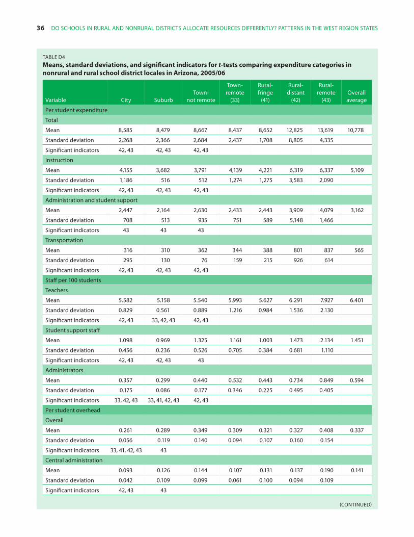
36 do SchoolS in rural and nonrural diSTricTS allocaTe reSourceS differenTly? paTTernS in The WeST region STaTeS
Table d4
means, standard deviations, and significant indicators for t-nonrural and rural school district locales in Arizona, 2005/06
tests comparing expenditure categories in
Town-Variable city Suburb not remote
Town-remote
(33)
rural-fringe
(41)
rural-distant
(42)
rural-remote
(43)overall average
per student expenditure
Total
mean 8,585 8,479 8,667 8,437 8,652 12,825 13,619 10,778
Standard deviation 2,268 2,366 2,684 2,437 1,708 8,805 4,335
Significant indicators 42, 43 42, 43 42, 43
instruction
mean 4,155 3,682 3,791 4,139 4,221 6,319 6,337 5,109
Standard deviation 1,186 516 512 1,274 1,275 3,583 2,090
Significant indicators 42, 43 42, 43 42, 43
administration and student support
mean 2,447 2,164 2,630 2,433 2,443 3,909 4,079 3,162
Standard deviation 708 513 935 751 589 5,148 1,466
Significant indicators 43 43 43
Transportation
mean 316 310 362 344 388 801 837 565
Standard deviation 295 130 76 159 215 926 614
Significant indicators 42, 43 42, 43 42, 43
Staff per 100 students
Teachers
mean 5.582 5.158 5.540 5.993 5.627 6.291 7.927 6.401
Standard deviation 0.829 0.561 0.889 1.216 0.984 1.536 2.130
Significant indicators 42, 43 33, 42, 43 42, 43
Student support staff
mean 1.098 0.969 1.325 1.161 1.003 1.473 2.134 1.451
Standard deviation 0.456 0.236 0.526 0.705 0.384 0.681 1.110
Significant indicators 42, 43 42, 43 43
administrators
mean 0.357 0.299 0.440 0.532 0.443 0.734 0.849 0.594
Standard deviation 0.175 0.086 0.177 0.346 0.225 0.495 0.405
Significant indicators 33, 42, 43 33, 41, 42, 43 42, 43
per student overhead
overall
mean 0.261 0.289 0.349 0.309 0.321 0.327 0.408 0.337
Standard deviation 0.056 0.119 0.140 0.094 0.107 0.160 0.154
Significant indicators 33, 41, 42, 43 43
central administration
mean 0.093 0.126 0.144 0.107 0.131 0.137 0.190 0.141
Standard deviation 0.042 0.109 0.099 0.061 0.100 0.094 0.109
Significant indicators 42, 43 43
(conTinued)

appendix d. reSulTS of pair-WiSe compariSonS for diSTricT localeS 37
Table d4 (conTinued)
means, standard deviations, and significant indicators for t-tests comparing expenditure categorienonrural and rural school district locales in Arizona, 2005/06
s in
Town- rural- rural- rural-Town- remote fringe distant remote
Variable city Suburb not remote (33) (41) (42) (43)overall average
operations and maintenance
mean 0.169 0.164 0.205 0.202 0.190 0.190 0.224 0.197
Standard deviation 0.027 0.029 0.051 0.041 0.049 0.079 0.070
Significant indicators 33, 43 33, 41, 43
Note: Significant indicators list the locale codes with statistically significant differences in the cell mean from that of the column-specific locale percent level.
at the 5
Source: Authors’ analysis based on data from U.S. Department of Education (2006a,b); http://nces.ed.gov/ccd/rural_locales.asp.

38 do SchoolS in rural and nonrural diSTricTS allocaTe reSourceS differenTly? paTTernS in The WeST region STaTeS
Table d5
means, standard deviations, and significant indicators for t-tests comparing contextual variables in nonrural and rural school district locales in california, 2005/06
Town- rural- rural- rural-Town-not remote fringe distant remote overall
Variable city Suburb remote (33) (41) (42) (43) average
district enrollment
mean 21,031 8,933 2,910 1,789 1,371 510 296 6,427
Standard deviation 62,540 10,293 2,374 1,655 2,957 926 569
Significant indicators 33, 41, 42, 43 33, 41, 42, 43 33, 41, 42, 43
Student population density within district
mean 453.70 398.51 30.36 19.47 24.43 4.49 2.40 190.09
Standard deviation 442.06 578.42 53.10 39.91 41.74 5.97 15.96
Significant indicators 33, 41, 42, 43 33, 41, 42, 43 42, 43
drive time from district to nearest urban area/cluster (minutes)
mean 11 19 5 5 11 24 60 19
Standard deviation 14 13 10 14 16 29 45
Significant indicators 33, 42, 43 33, 41, 43 41, 42, 43
percentage of students living in poverty
mean 15.54 12.88 20.61 18.78 15.84 18.78 20.84 16.6
Standard deviation 8.45 7.76 9.61 4.83 9.63 9.39 9.10
Significant indicators 33, 42, 43 33, 41, 42, 43 41 16.6
percentage of students identified as english language learner students
mean 24.71 18.25 24.22 11.61 16.15 16.82 8.74 18.36
Standard deviation 16.56 15.09 20.57 15.75 18.48 20.48 18.49
Significant indicators 33, 41, 42, 43 33, 43 33, 41, 42, 43
percentage of students identified as having individualized education program
mean 9.92 9.69 8.83 11.43 7.05 5.79 6.65 8.39
Standard deviation 2.12 2.72 4.08 4.66 5.55 5.72 6.99
Significant indicators 41, 42, 43 33, 41, 42, 43 33, 41, 42, 43
comparable Wage index
mean 1.362 1.353 1.168 0.948 1.223 1.178 0.988 1.235
Standard deviation 0.167 0.122 0.182 0.133 0.199 0.202 0.197
Significant indicators 33, 41, 42, 43 33, 41, 42, 43 33, 41, 43
Note: Significant indicators list the locale codes with statistically significant differences in the cell mean from that of the column-specific locale at the 5 percent level.
Source: Authors’ analysis based on data from U.S. Department of Education (2005, 2006a); U.S. Census Bureau (2000, 2005); http://nces.ed.gov/ccd/rural_locales.asp.
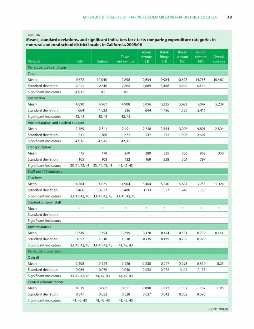
appendix d. reSulTS of pair-WiSe compariSonS for diSTricT localeS 39
Table d6
means, standard deviations, and significant indicators for t-tnonrural and rural school district locales in california, 2005/
ests com06
paring expenditure categories in
Town-Variable city Suburb not remote
Town-remote
(33)
rural-fringe
(41)
rural-distant
(42)
rural-remote
(43)overall average
per student expenditure
Total
mean 9,672 10,040 9,898 9,634 9,984 10,628 14,765 10,462
Standard deviation 2,091 2,819 2,865 2,689 3,468 3,699 6,468
Significant indicators 42, 43 43 43
instruction
mean 4,890 4,987 4,908 5,056 5,125 5,421 7,047 5,239
Standard deviation 664 1,023 826 644 1,426 1,556 2,416
Significant indicators 42, 43 42, 43 42, 43
administration and student support
mean 2,469 2,541 2,491 2,518 2,544 3,026 4,801 2,804
Standard deviation 541 788 672 717 932 1,306 2,607
Significant indicators 42, 43 42, 43 42, 43
Transportation
mean 175 170 250 289 325 506 962 330
Standard deviation 105 108 132 169 228 324 797
Significant indicators 33, 41, 42, 43 33, 41, 42, 43 41, 42, 43
Staff per 100 students
Teachers
mean 4.764 4.835 4.964 5.464 5.310 5.631 7.755 5.324
Standard deviation 0.466 0.633 0.480 1.113 1.037 1.248 3.153
Significant indicators 33, 41, 42, 43 33, 41, 42, 43 33, 41, 42, 43
Student support staffa a amean a a a a a
Standard deviation
Significant indicators
administrators
mean 0.349 0.354 0.399 0.420 0.474 0.581 0.739 0.444
Standard deviation 0.092 0.110 0.118 0.135 0.199 0.259 0.270
Significant indicators 33, 41, 42, 43 33, 41, 42, 43 41, 42, 43
per student overhead
overall
mean 0.208 0.224 0.226 0.230 0.247 0.298 0.360 0.25
Standard deviation 0.065 0.070 0.050 0.053 0.072 0.112 0.173
Significant indicators 33, 41, 42, 43 41, 42, 43 41, 42, 43
central administration
mean 0.079 0.087 0.091 0.090 0.112 0.137 0.162 0.105
Standard deviation 0.041 0.033 0.028 0.027 0.042 0.052 0.090
Significant indicators 41, 42, 43 41, 42, 43 41, 42, 43
(conTinued)
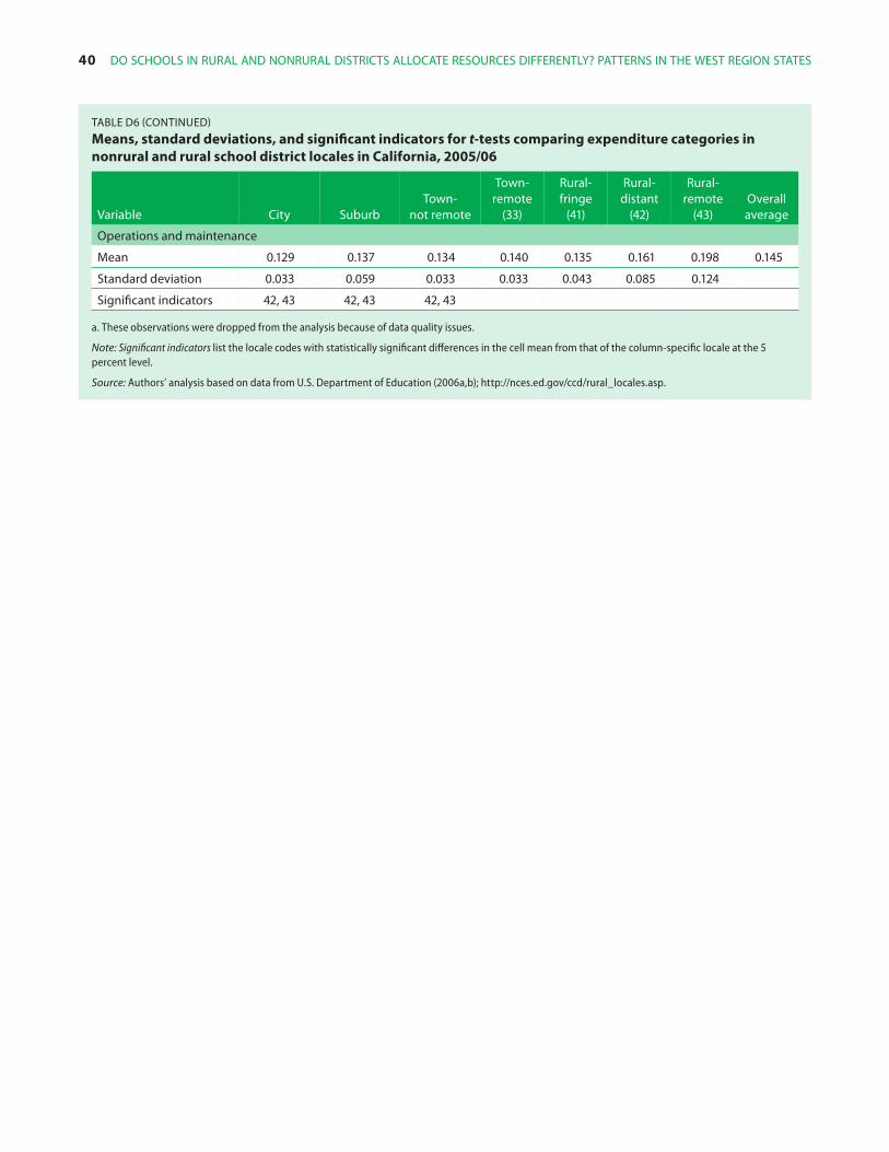
40 do SchoolS in rural and nonrural diSTricTS allocaTe reSourceS differenTly? paTTernS in The WeST region STaTeS
Table d6 (conTinued)
means, standard deviations, and significant indicators for t-tests comparing expenditure categorienonrural and rural school district locales in california, 2005/06
s in
Town- rural- rural- rural-Town- remote fringe distant remote
Variable city Suburb not remote (33) (41) (42) (43)overall average
operations and maintenance
mean 0.129 0.137 0.134 0.140 0.135 0.161 0.198 0.145
Standard deviation 0.033 0.059 0.033 0.033 0.043 0.085 0.124
Significant indicators 42, 43 42, 43 42, 43
a. These observations were dropped from the analysis because of data quality issues.
Note: Significant indicators list the locale codes with statistically significant differences in the cell mean from that of the column-specific locale percent level.
at the 5
Source: Authors’ analysis based on data from U.S. Department of Education (2006a,b); http://nces.ed.gov/ccd/rural_locales.asp.

appendix d. reSulTS of pair-WiSe compariSonS for diSTricT localeS 41
Table d7
means, standard deviations, and significant indicators for and rural school district locales in nevada, 2005/06
t-tests comparing contextual variables in nonrural
Town-Variable city Suburb not remote
Town- rural- rural- rural-remote fringe distant remote overall
(33) (41) (42) (43) average
district enrollment
mean 36,677 294,131 7,841 3,927 3,689 450 530 24,279
Standard deviation 38,989 a 1,226 3,580 3,446 a 441
Significant indicators 42 33, 41, 42, 43 42
Student population density within district
mean 34.18 36.35 6.89 0.45 0.24 1.71 0.08 7.25
Standard deviation 34.47 a 3.63 0.30 0.14 a 0.05
Significant indicators 42 33, 41, 42, 43 42
drive time from district to nearest urban area/cluster (minutes)
mean 31 31 47 18 144 22 146 69
Standard deviation 11 a 37 40 201 a 55
Significant indicators 42, 43 33, 41, 42, 43 42
percentage of students living in poverty
mean 11.86 14.10 9.89 13.90 15.17 5.74 12.85 12.62
Standard deviation 0.75 a 2.08 4.89 3.58 a 2.58
Significant indicators 42 33, 41, 42, 43 42
percentage of students identified as english language learner students
mean 15.64 17.26 5.18 3.18 4.09 0.00 4.02 5.83
Standard deviation 1.91 a 0.28 3.25 4.65 a 3.86
Significant indicators 33, 42, 43 33, 41, 42, 43 42
percentage of students identified as having individualized education program
mean 12.06 10.78 10.84 10.09 9.59 21.78 9.63 10.97
Standard deviation 1.53 a 0.22 3.60 0.13 a 5.34
Significant indicators 42 33, 41, 42, 43 41, 42
comparable Wage index
mean 1.186 1.306 1.151 1.095 1.095 1.221 1.095 1.132
Standard deviation 0.049 a 0.000 0.000 0.000 a 0.000
Significant indicators 42 33, 41, 42, 43 33, 41, 42, 43
a. Standard deviation is not defined because cell represents a single district.
Note: Significant indicators list the locale codes with statistically significant differences in the cell mean from that of the column-specific locale at the 5 percent level.
Source: Authors’ analysis based on data from U.S. Department of Education (2005, 2006a); U.S. Census Bureau (2000, 2005); http://nces.ed.gov/ccd/rural_locales.asp.
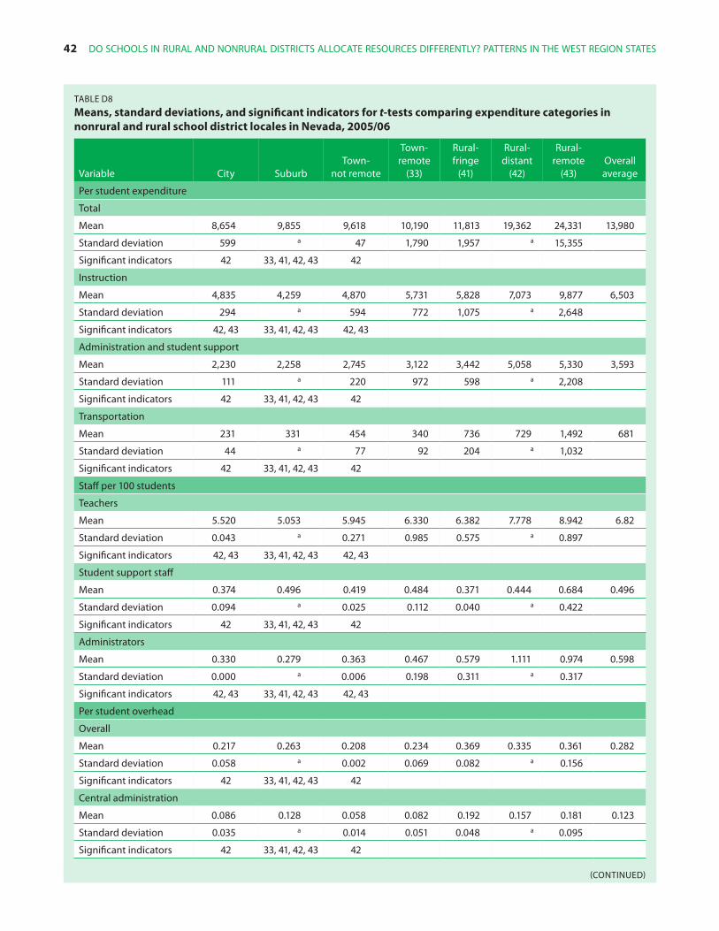
42 do SchoolS in rural and nonrural diSTricTS allocaTe reSourceS differenTly? paTTernS in The WeST region STaTeS
Table d8
means, standard deviations, and snonrural and rural school district
ignificant indicators for t-tlocales in nevada, 2005/06
ests comparing expenditure categories in
Variable cityTown-
Suburb not remote
Town-remote
(33)
rural-fringe
(41)
rural-distant
(42)
rural-remote
(43)overall average
per student expenditure
Total
mean 8,654 9,855 9,618 10,190 11,813 19,362 24,331 13,980
Standard deviation 599 a 47 1,790 1,957 a 15,355
Significant indicators 42 33, 41, 42, 43 42
instruction
mean 4,835 4,259 4,870 5,731 5,828 7,073 9,877 6,503
Standard deviation 294 a 594 772 1,075 a 2,648
Significant indicators 42, 43 33, 41, 42, 43 42, 43
administration and student support
mean 2,230 2,258 2,745 3,122 3,442 5,058 5,330 3,593
Standard deviation 111 a 220 972 598 a 2,208
Significant indicators 42 33, 41, 42, 43 42
Transportation
mean 231 331 454 340 736 729 1,492 681
Standard deviation 44 a 77 92 204 a 1,032
Significant indicators 42 33, 41, 42, 43 42
Staff per 100 students
Teachers
mean 5.520 5.053 5.945 6.330 6.382 7.778 8.942 6.82
Standard deviation 0.043 a 0.271 0.985 0.575 a 0.897
Significant indicators 42, 43 33, 41, 42, 43 42, 43
Student support staff
mean 0.374 0.496 0.419 0.484 0.371 0.444 0.684 0.496
Standard deviation 0.094 a 0.025 0.112 0.040 a 0.422
Significant indicators 42 33, 41, 42, 43 42
administrators
mean 0.330 0.279 0.363 0.467 0.579 1.111 0.974 0.598
Standard deviation 0.000 a 0.006 0.198 0.311 a 0.317
Significant indicators 42, 43 33, 41, 42, 43 42, 43
per student overhead
overall
mean 0.217 0.263 0.208 0.234 0.369 0.335 0.361 0.282
Standard deviation 0.058 a 0.002 0.069 0.082 a 0.156
Significant indicators 42 33, 41, 42, 43 42
central administration
mean 0.086 0.128 0.058 0.082 0.192 0.157 0.181 0.123
Standard deviation 0.035 a 0.014 0.051 0.048 a 0.095
Significant indicators 42 33, 41, 42, 43 42
(conTinued)

appendix d. reSulTS of pair-WiSe compariSonS for diSTricT localeS 43
Table d8 (conTinued)
means, standard deviations, and significant indicators for t-tests comparing expenditure categorienonrural and rural school district locales in nevada, 2005/06
s in
Town- rural- rural- rural-Town- remote fringe distant remote
Variable city Suburb not remote (33) (41) (42) (43)overall average
operations and maintenance
mean 0.131 0.136 0.150 0.152 0.177 0.178 0.180 0.159a aStandard deviation 0.023 0.015 0.029 0.035 0.064
Significant indicators 42 33, 41, 42, 43 42
a. Standard deviation is not defined because cell represents a single district.
Note: Significant indicators list the locale codes with statistically significant differences in the cell mean from that of the column-specific locale percent level.
at the 5
Source: Authors’ analysis based on data from U.S. Department of Education (2006a,b); http://nces.ed.gov/ccd/rural_locales.asp.

44 do SchoolS in rural and nonrural diSTricTS allocaTe reSourceS differenTly? paTTernS in The WeST region STaTeS
Table d9
means, standard deviations, and significant indicators for t-tests comparing contextual variables in nonrural and rural school district locales in utah, 2005/06
Town- rural- rural- rural-Town- remote fringe distant remote overall
Variable city Suburb not remote (33) (41) (42) (43) average
district enrollment
mean 15,812 44,333 11,065 3,650 2,028 2,034 1,425 12,413a aStandard deviation 7,917 27,868 8,057 2,007 1,225
Significant indicators 33, 41, 42, 43 33, 41, 42, 43 41, 42
Student population density within district
mean 928.05 183.03 14.66 1.49 1.71 3.33 0.91 150.59a aStandard deviation 1,457.00 226.12 20.42 1.03 1.14
Significant indicators 41, 42 41, 42 41, 42
drive time from district to nearest urban area/cluster (minutes)
mean 17 15 8 2 0 40 64 28a aStandard deviation 25 7 11 6 43
Significant indicators 41, 42, 43 33, 41, 42, 43 41, 42, 43
percentage of students living in poverty
mean 16.48 7.51 7.13 17.07 10.90 4.79 12.93 12.27a aStandard deviation 3.98 1.65 1.16 6.06 4.37
Significant indicators 41, 42 33, 41, 42, 43 33, 41, 42, 43
percentage of students identified as english language learner students
mean 20.39 7.55 6.98 5.26 0.00 0.39 3.91 7.07a aStandard deviation 10.38 7.39 3.07 6.03 2.97
Significant indicators 33, 41, 42, 43 41, 42 41, 42
percentage of students identified as having individualized education program
mean 13.49 12.72 14.00 16.46 14.50 7.72 15.18 14.44a aStandard deviation 0.70 1.72 1.70 3.07 2.71
Significant indicators 33, 41, 42 33, 41, 42, 43 41, 42
comparable Wage index
mean 1.134 1.172 1.155 1.041 1.179 1.155 1.075 1.107a aStandard deviation 0.074 0.024 0.052 0.035 0.076
Significant indicators 33, 41, 42 33, 41, 42, 43 33, 41, 42, 43
a. Standard deviation is not defined because cell represents a single district.
Note: Significant indicators list the locale codes with statistically significant differences in the cell mean from that of the column-specific locale at the 5 percent level.
Source: Authors’ analysis based on data from U.S. Department of Education (2005, 2006a); U.S. Census Bureau (2000, 2005); http://nces.ed.gov/ccd/rural_locales.asp.
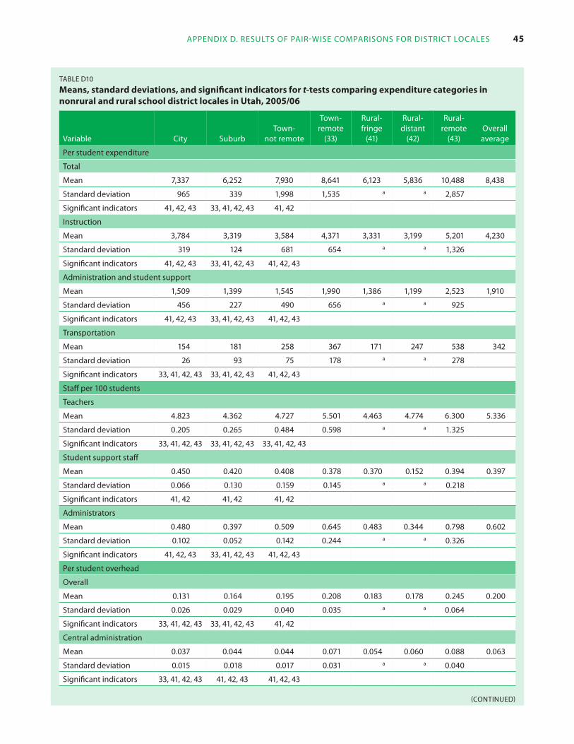
appendix d. reSulTS of pair-WiSe compariSonS for diSTricT localeS 45
Table d10
means, standard deviations, and significant indicators for t-tnonrural and rural school district locales in utah, 2005/06
ests comparing expenditure categories in
Town-Variable city Suburb not remote
Town-remote
(33)
rural-fringe
(41)
rural-distant
(42)
rural-remote
(43)overall average
per student expenditure
Total
mean 7,337 6,252 7,930 8,641 6,123 5,836 10,488 8,438
Standard deviation 965 339 1,998 1,535 a a 2,857
Significant indicators 41, 42, 43 33, 41, 42, 43 41, 42
instruction
mean 3,784 3,319 3,584 4,371 3,331 3,199 5,201 4,230
Standard deviation 319 124 681 654 a a 1,326
Significant indicators 41, 42, 43 33, 41, 42, 43 41, 42, 43
administration and student support
mean 1,509 1,399 1,545 1,990 1,386 1,199 2,523 1,910
Standard deviation 456 227 490 656 a a 925
Significant indicators 41, 42, 43 33, 41, 42, 43 41, 42, 43
Transportation
mean 154 181 258 367 171 247 538 342
Standard deviation 26 93 75 178 a a 278
Significant indicators 33, 41, 42, 43 33, 41, 42, 43 41, 42, 43
Staff per 100 students
Teachers
mean 4.823 4.362 4.727 5.501 4.463 4.774 6.300 5.336
Standard deviation 0.205 0.265 0.484 0.598 a a 1.325
Significant indicators 33, 41, 42, 43 33, 41, 42, 43 33, 41, 42, 43
Student support staff
mean 0.450 0.420 0.408 0.378 0.370 0.152 0.394 0.397
Standard deviation 0.066 0.130 0.159 0.145 a a 0.218
Significant indicators 41, 42 41, 42 41, 42
administrators
mean 0.480 0.397 0.509 0.645 0.483 0.344 0.798 0.602
Standard deviation 0.102 0.052 0.142 0.244 a a 0.326
Significant indicators 41, 42, 43 33, 41, 42, 43 41, 42, 43
per student overhead
overall
mean 0.131 0.164 0.195 0.208 0.183 0.178 0.245 0.200
Standard deviation 0.026 0.029 0.040 0.035 a a 0.064
Significant indicators 33, 41, 42, 43 33, 41, 42, 43 41, 42
central administration
mean 0.037 0.044 0.044 0.071 0.054 0.060 0.088 0.063
Standard deviation 0.015 0.018 0.017 0.031 a a 0.040
Significant indicators 33, 41, 42, 43 41, 42, 43 41, 42, 43
(conTinued)

46 do SchoolS in rural and nonrural diSTricTS allocaTe reSourceS differenTly? paTTernS in The WeST region STaTeS
Table d10 (conTinued)
means, standard deviations, and significant indicators for t-tests comparing expenditure nonrural and rural school district locales in utah, 2005/06
categories in
Town- rural- rural-Town- remote fringe distant
Variable city Suburb not remote (33) (41) (42)
rural-remote
(43)overall average
operations and maintenance
mean 0.093 0.121 0.152 0.137 0.129 0.117 0.157 0.136a aStandard deviation 0.036 0.015 0.028 0.028 0.039
Significant indicators 41, 42, 43 41, 42, 43 41, 42
a. Standard deviation is not defined because cell represents a single district.
Note: Significant indicators list the locale codes with statistically significant differences in the cell mean from that of the column-spercent level.
pecific locale at the 5
Source: Authors’ analysis based on data from U.S. Department of Education (2006a,b); http://nces.ed.gov/ccd/rural_locales.asp.
Table D11 summarizes the t-test results for the 10 resource measures investigated. All but one compar-ison for staffing ratios was highly significant. (The exception is student support staff, which does not include California school districts, which represent more than two-thirds of the sample.) The most sig-nificant differences are in teacher staffing ratios and
transportation expenditures. Significant differences are found between rural-distant and rural-remote school districts, suggesting that the locale taxonomy applied to the West Region does not align perfectly with the gradations seen in resource allocation pat-terns of school districts. In other words, the majority of the categories look more alike than different.
Table d11
p-values for nonrural to rural t-test results for all resource measures for all significant differences
per student expenditures Staff per 100 students per student overhead
Admini-stration
and Student Instruc- student Transpor- support Admini-
locale Total tion support tation Teachers staff strators Overall
Central adminis-tration
Opera-tions and mainte-nance
urban compared with
Town-remote <.001 <.001 <.001
rural-fringe <.05 <.001 <.001 <.001
rural-distant <.001 <.001 <.001 <.001 <.001 <.01 <.001
rural-remote <.001 <.001 <.001 <.001 <.001 <.001 <.001
<.001
<.001
<.001
<.001
<.05
<.001
<.001
<.001
<.001
<.05
<.001
<.001
Suburb compared with
Town-remote <.05 <.001 <.001 <.001
rural-fringe <.001 <.001 <.001
rural-distant <.01 <.001 <.001 <.001 <.001 <.001 <.001
rural-remote <.001 <.001 <.001 <.001 <.001 <.001 <.001
<.01
<.001
<.001
<.001
<.001
<.001
<.001
<.001
<.001
<.001
Town-not remote compared with
Town-remote <.05 <.001 <.05
rural-fringe <.001 <.001 <.001
rural-distant <.01 <.001 <.001 <.001 <.001 <.05 <.001
rural-remote <.001 <.001 <.001 <.001 <.001 <.001 <.001
number significant 7 7 6 12 12 6 12
Source: Authors’ analysis based on data from U.S. Department of Education (2006a,b); http://nces.ed.gov/ccd/rural_l
<.01
<.001
<.001
11
ocales.asp.
<.001
<.001
<.001
10
<.01
<.001
<.001
10
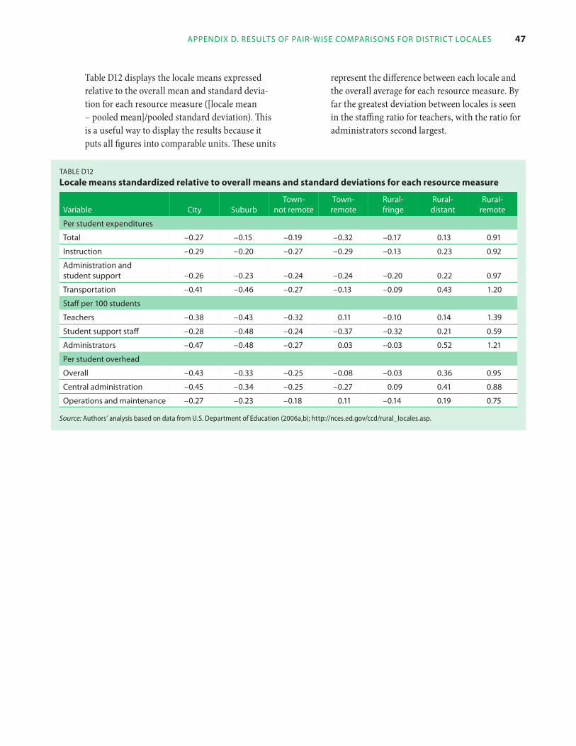
appendix d. reSulTS of pair-WiSe compariSonS for diSTricT localeS 47
Table D12 displays the locale means expressed relative to the overall mean and standard devia-tion for each resource measure ([locale mean – pooled mean]/pooled standard deviation). This is a useful way to display the results because it puts all figures into comparable units. These units
represent the difference between each locale and the overall average for each resource measure. By far the greatest deviation between locales is seen in the staffing ratio for teachers, with the ratio for administrators second largest.
Table d12
locale means standardized relative to overall means and standard deviations for each resource measure
Variable city SuburbTown-
not remoteTown-
remoterural- fringe
rural-distant
rural-remote
per student expenditures
Total –0.27 –0.15 –0.19 –0.32 –0.17 0.13 0.91
instruction –0.29 –0.20 –0.27 –0.29 –0.13 0.23 0.92
administration and student support –0.26 –0.23 –0.24 –0.24 –0.20 0.22 0.97
Transportation –0.41 –0.46 –0.27 –0.13 –0.09 0.43 1.20
Staff per 100 students
Teachers –0.38 –0.43 –0.32 0.11 –0.10 0.14 1.39
Student support staff –0.28 –0.48 –0.24 –0.37 –0.32 0.21 0.59
administrators –0.47 –0.48 –0.27 0.03 –0.03 0.52 1.21
per student overhead
overall –0.43 –0.33 –0.25 –0.08 –0.03 0.36 0.95
central administration –0.45 –0.34 –0.25 –0.27 0.09 0.41 0.88
operations and maintenance –0.27 –0.23 –0.18 0.11 –0.14 0.19 0.75
Source: Authors’ analysis based on data from U.S. Department of Education (2006a,b); http://nces.ed.gov/ccd/rural_locales.asp.

48 do SchoolS in rural and nonrural diSTricTS allocaTe reSourceS differenTly? paTTernS in The WeST region STaTeS
APPenDix e missing AnD RecoDeD RecoRDs AnD vARiAbles
Several variables from both the National Center for Education Statistics Common Core of Data and its School District Finance Survey (F-33) were found to contain implausible zero values (U.S. Department of Education 2006a,b). These values were set to “missing” in order to omit them from analyses.
Tables E1–E5 show the counts and percentages of districts (and corresponding student populations) dropped because of reported zero values, by locale category. In all cases except student support staff (table E3), the number of cases dropped from both the descriptive and the regression analyses is equal to the number of records containing zero values. For California, all records were omitted from the descriptive analysis of student support staff because 24 percent of the districts in the state reported zero student support staff. Regression analysis for student support staff across all districts was not performed.
Table e1
Districts and students dropped from analysis of per student trancalifornia, 2005/06
sportation expenditures in Arizona and
districts Students
dropped retainedState and locale dropped retained
category number percent number percent number percent number percent
arizona
rural-remote 1 1.6 61 98.4 78 0.3 23,987 99.7
california
city 1 0.7 140 99.3 300 0.0 2,965,837 100.0
rural-distant 15 10.0 135 90.0 1,134 1.5 75,430 98.5
rural-fringe 19 13.2 125 86.8 4,213 2.1 195,652 97.9
rural-remote 5 5.8 81 94.2 200 0.8 25,930 99.2
Suburb 17 6.2 256 93.8 22,322 0.9 2,420,385 99.1
Town-not remote 1 0.8 125 99.2 124 0.0 368,080 100.0
Source: Authors’ analysis based on data from U.S. Department of Education (2006a,b); http://nces.ed.gov/ccd/rural_locales.asp.
Table e2
Districts and students dropped from analysis of teacher staffing ratio in Arizona and california, 2005/06
districts Students
State and locale dropped retained dropped retained
category number percent number percent number percent number percent
arizona
rural-remote 1 1.6 61 98.4 78 0.3 23,987 99.7
california
Town-not remote 1 0.8 125 99.2 124 0.0 368,080 100.0
Source: Authors’ analysis based on data from U.S. Department of Education (2006a); http://nces.ed.gov/ccd/rural_locales.asp.

appendix e. miSSing and recoded recordS and VariableS 49
Table e3
Districts and stud2005/06
ents dropped from analysis of student support staffing ratio in Arizona and california,
districts Students
State and locale dropped retained dropped retained
category number percent number percent number percent number percent
arizona
rural-distant 3 8.8 31 91.2 31 0.1 38,214 99.9
rural-fringe 1 3.8 25 96.2 145 0.2 59,260 99.8
rural-remote 6 9.7 56 90.3 274 1.1 23,791 98.9
california
city 4 2.8 137 97.2 1,868 0.1 2,964,269 99.9
rural-distant 85 56.7 65 43.3 15,870 20.7 60,694 79.3
rural-fringe 62 43.1 82 56.9 18,655 9.3 181,210 90.7
rural-remote 54 62.8 32 37.2 5,116 19.6 21,014 80.4
Suburb 11 4.0 262 96.0 5,508 0.2 2,437,199 99.8
Town-not remote 8 6.3 118 93.7 5,036 1.4 363,168 98.6
Town-remote 4 11.8 30 88.2 1,434 2.4 59,408 97.6
Source: Authors’ analysis based on data from U.S. Department of Education (2006a); http://nces.ed.gov/ccd/rural_locales.asp.
Table e4
Districts and students dropped from analysis of administrator staffing ratio in Arizona and california, 2005/06
districts Students
State and locale dropped retained dropped retained
category number percent number percent number percent number percent
arizona
rural-remote 2 3.2 60 96.8 201 0.8 23,864 99.2
california
rural-distant 16 10.7 134 89.3 1,369 1.8 75,195 98.2
rural-fringe 9 6.3 135 93.8 539 0.3 199,326 99.7
rural-remote 13 15.1 73 84.9 504 1.9 25,626 98.1
Suburb 1 0.4 272 99.6 587 0.0 2,442,120 100.0
Source: Authors’ analysis based on data from U.S. Department of Education (2006a); http://nces.ed.gov/ccd/rural_locales.asp.
Table e5
Districts and students dropped from analysis of central adminicalifornia, 2005/06
stration overhead ratio in Arizona and
districts Students
dropped retainedState and locale dropped retained
category number percent number percent number percent number percent
arizona
rural-remote 2 3.2 60 96.8 174 0.7 23,891 99.3
Source: Authors’ analysis based on data from U.S. Department of Education (2006a,b); http://nces.ed.gov/ccd/rural_locales.asp.

50 do SchoolS in rural and nonrural diSTricTS allocaTe reSourceS differenTly? paTTernS in The WeST region STaTeS
APPenDix f RegRession AnAlysis meThoDology AnD moDels
The analysis focused on the variations in the resource measures associated with three re-gional characteristics — district enrollment (size), student population density in the district, and average drive time from the school district’s central office to the nearest urban area/cluster — while controlling for variations in student needs and regional variations in the cost of labor. Specifically, using ordinary least squares regres-sion models, the study explored the relationship between these characteristics of districts and three resource measures: per student expendi-tures (overall, instructional, and student support services); staff per 100 students (for teachers and administrators); and overhead ratios in different configurations.
The final regression model was obtained by re-gressing total per student expenditure on student needs (percentage of students eligible for free or reduced-price lunch, percentage of English language learner students, and percentage of stu-dents with Individualized Education Programs); staffing cost levels (Comparable Wage Index); and regional characteristics (district size, student population density, and drive time to nearest urban area/cluster) in turn. Differences across states in the relationship between the resource measures and the cost factors were accounted for by including interactions between the state indicators and each control variable (see detailed specification below).
Although the study data included the full popu-lation of school districts in the West Region in 2005/06, this finite population represents a single snapshot (sample) of the superpopulation of all combinations of observed districts in the region over time. Estimation methods that take into account sampling error are appropriate in this context (see Deming and Stephan 1941).
Regression model specification
The regression specification used in the analysis took the following form:
3 3ln(Yd) = α + Σ βjln(1 + Xj,d) + Σ βkln(Xk,d) +
j=1 k=13 3 3
βlDd + Σ δsSs,d + Σ Σ φj,s[ln(1 + Xj,d)Ss,d] + s=2 j=1s=2
3 3 3Σ Σ φk,s[ln(Xk,d)Ss,d] + Σ φl,sDdSs,d + εdk=1s=2 s=2
where Y is a resource allocation measure (expen-diture, staffing ratio, overhead ratio); S represents dichotomous dummy indicator variables denot-ing state s (2 = Arizona, 3 = Utah, and California serves as the omitted reference group); Xj is a matrix of j independent variables denoting student needs, including the district percentage of the school-age population in poverty according to U.S. Census Bureau Small Area Income Population Estimates (SAIPE), the district-level percentage of students designated as English language learner students, and the district-level percentage of special education students, or students with Individual-ized Education Programs (adding 1 to the student needs cost factors was necessary because some districts could have a zero value, which would be undefined in log form); Xk is a matrix of K inde-pendent variables denoting district enrollment, student population density, and the Comparable Wage Index; D is drive time to nearest urban area/cluster; α, β, δ, and φ are regression coefficients; ε is a random error term assumed to be independently and identically distributed across districts; and d is a subscript denoting district-specific observations.
Example of calculating differentials in resource utilization
The estimated regression models were used to ana-lyze how predicted resource utilization varied for each regional characteristic while holding all other cost factors constant at their sample means. In this way it was possible to calculate expected differ-ences in resource allocation associated with a given characteristic for the “average” (in the sense that all other cost factors were set at their average across all districts in the sample) district in the region.

appendix f. regreSSion analySiS meThodology and modelS 51
Consider a modified version of the model in which one of the three regional characteristics (Xl,d) of interest, such as district enrollment, is identified. The corresponding estimated model to predict val-ues of overall per student expenditure for different levels of district enrollment while setting all other covariates to their sample means is as follows:
3ln(̂
2Yd) = α̂ + Σ β̂jln(1 + Xj,d) + Σ β̂kln(Xk,d) +
j=1 k=1ˆ ˆ 3 ˆ 3 3βlln(Xl,d) + βmDd + Σ δsSs,d + Σ Σ φj,s[ln(1 + Xj,d)Ss,d] +
s=2 j=1s=22 3 3 3Σ Σ φ̂k,s[ln(Xk,d)Ss,d] + Σ φ̂l,s [ln(Xl,d)Ss,d] + Σ φ̂m,sDdSs,d.k=1s=2 s=2 s=2
Table F1 shows how the example of differential overall per student expenditure between two
Table f1
example of predicted differentials in overall per student expenditures as2005/06
sociated with district enrollment,
(3)(2) Transformations
(1) Sample means to variable values raw cost model with enrollment used in model factors coefficients set to 296 predictions
(4)Transformed
raw cost factor values for model
predictions
(5)coefficients times
transformed values
enrollment = 296
california indicator 10.021 1.000 none 1.000 10.021
poverty 0.102 0.1757 ln(1+poverty) 0.162 0.017
english language learner student (ell) 0.08 0.172 ln(1+ell) 0.159 0.013
Special education ln(1+Special student 0.983 0.1056 education) 0.100 0.099
comparable Wage index (cWi) 0.211 1.20 ln(cWi) 0.182 0.038
–0.246 ln(enrollment)enrollment 296
0.015 ln(enrollment)2
5.690 –1.400
32.380 0.486
Student density –0.022 168.81 ln(Student density) 5.129 –0.113
drive time 0.002 20.79 none 20.790 0.042
prediction = sum of coefficients times transformed values 9.202
prediction in dollars = exp(sum of coefficients times transformed values) $9,917
enrollment = 6,257
california indicator 10.021 1.000 none 1.000 10.021
poverty 0.102 0.1757 ln(1+poverty) 0.162 0.017
english language learner student (ell) 0.08 0.172 ln(1+ell) 0.159 0.013
Special education ln(1+Special 0.983 0.1056 education) 0.100 0.099
comparable Wage index (cWi) 0.211 1.20 ln(cWi) 0.182 0.038
–0.246 ln(enrollment)enrollment 6,427
0.015 ln(enrollment)2
8.768 –2.157
76.882 1.153
Student density –0.022 168.81 ln(Student density) 5.129 –0.113
drive time 0.002 20.79 none 20.790 0.042
prediction = sum of coefficients times transformed values 9.112
prediction in dollar terms = exp(sum of coefficients times transformed values) $9,067
Source: Authors’ analysis based on data from U.S. Department of Education (2005, 2006a,b); U.S. Census Bureau (2000, 2005).

52 do SchoolS in rural and nonrural diSTricTS allocaTe reSourceS differenTly? paTTernS in The WeST region STaTeS
California districts with varying enrollment levels presented in the main text was calculated. The first column displays an abridged set of regres-sion coefficients from the estimated overall per student expenditure model (taken from table G1 in appendix G). In the second column, all raw cost factors in the model except enrollment were set equal to their sample means across all districts in the West Region. In the first panel, enrollment was set to 296; in the second panel enrollment was set to 6,257. Using the transformations defined in the third column, the figures from column 2 were changed into the variable values used in the model (column 4). They were multiplied by the estimated model coefficients to provide the numbers in column 5.
In each panel the multiplied figures were summed to provide the model predictions for the expected overall per student expenditure associated with the two enrollment levels. Because the model uses the natural logarithm of overall per student expenditure as the dependent variable, antilogs of the model predictions must be taken to come up with the dollar values for the overall per student expenditures stemming from each scenario. Doing so yields predicted overall per student expenditure of $9,917 (equal to exp[9.202]) for a district with enrollment of 296 and $9,067 (equal to exp[9.112]) for a district with enrollment of 6,257. Predictions for the other states are made in a similar fashion, but they are slightly more involved because the coefficients associated with the appropriate state interaction terms must also be considered.

appendix g. regreSSion model reSulTS 53
APPenDix g RegRession moDel ResulTs
Table g1
Development of final regression model using overall per student expenditures in 2005/06 as dependent variable
Variable model 1 model 2 model 3 model 4 model 5 model 6model 7
(final)
model intercept (reference group is california) 9.210*** 9.127*** 10.175*** 10.065*** 10.132*** 9.959*** 10.021***
arizona 0.000 –0.057 –0.049* –0.147*** –0.153* 0.546** 0.466*
utah –0.207*** –0.215*** –0.212*** –0.225*** –0.707* 1.886 1.468
ln(1+poverty) 0.731*** 0.365** 0.081 0.333** 0.102
ln(1+ell) –0.382*** 0.025 0.118 0.032 0.080
ln(1+Special education) 0.168 0.974*** 1.142*** 0.821*** 0.983***
ln(cWi) 0.098 0.296*** 0.229*** 0.264*** 0.211***
ln(enrollment) –0.255*** –0.264*** –0.276*** –0.237*** –0.246***
ln(enrollment)2 0.016*** 0.016*** 0.017*** 0.015*** 0.015***
ln(Student density) –0.014** –0.022*** –0.021*** –0.022*** –0.022***
drive time 0.002*** 0.002*** 0.002*** 0.002*** 0.002***
ln(1+poverty)
arizona 1.049*** 0.004 0.908***
utah 1.475 0.025 –0.134
ln(1+ell)
arizona –0.413* –0.188
utah –0.103 1.257
ln(1+Special education)
arizona –1.061** –0.800*
utah 2.006 1.278
ln(cWi)
arizona 0.339 0.558*
utah 0.359 0.240
ln(enrollment)
arizona –0.161** –0.164**
utah –0.360 –0.333
ln(enrollment)2
arizona 0.008 0.009*
utah 0.013 0.012
ln(Student density)
arizona 0.000 0.000
utah –0.002 –0.002
drive time
arizona 0.000
utah 0.004
(conTinued)
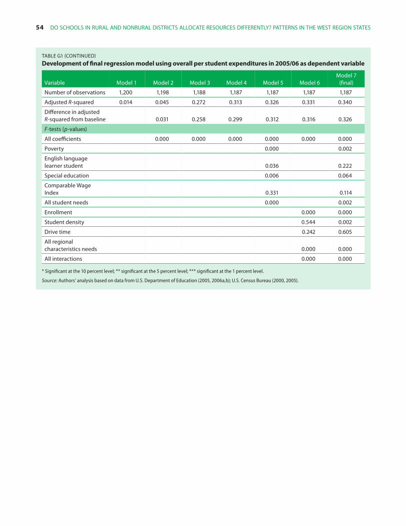
54 do SchoolS in rural and nonrural diSTricTS allocaTe reSourceS differenTly? paTTernS in The WeST region STaTeS
Table g1 (conTinued)
Development of final regression model using overall per student expenditures in 2005/06 as dependent variable
Variable model 1 model 2 model 3 model 4 model 5 model 6model 7
(final)
number of observations 1,200 1,198 1,188 1,187 1,187 1,187 1,187
adjusted R-squared 0.014 0.045 0.272 0.313 0.326 0.331 0.340
difference in adjusted R-squared from baseline 0.031 0.258 0.299 0.312 0.316 0.326
F-tests (p-values)
all coefficients 0.000 0.000 0.000 0.000 0.000 0.000
poverty 0.000 0.002
english language learner student 0.036 0.222
Special education 0.006 0.064
comparable Wage index 0.331 0.114
all student needs 0.000 0.002
enrollment 0.000 0.000
Student density 0.544 0.002
drive time 0.242 0.605
all regional characteristics needs 0.000 0.000
all interactions 0.000 0.000
* Significant at the 10 percent level; ** significant at the 5 percent level; *** significant at the 1 percent level.
Source: Authors’ analysis based on data from U.S. Department of Education (2005, 2006a,b); U.S. Census Bureau (2000, 2005).

appendix g. regreSSion model reSulTS 55
Table g2
Regressions of per student expenditures in West Region school districts, 2005/06
administration and student
Variable overall instruction support Transportation
model intercept (reference group is california) 10.0210*** 9.2640*** 9.8281*** 7.3135***
State-specific controls
arizona 0.4655* 1.0766*** 0.7374*** –0.5355
utah 1.4682 2.2583* 2.2740* 3.898
Student needs
ln(1+poverty)
main effect (california) 0.1021 0.0606 0.2178* 1.8761***
interactions
arizona 0.9083*** 0.5802*** 0.7280*** –1.9341**
utah –0.1344 0.4866 0.6598 –1.8067
ln(1+ell)
main effect (california) 0.0801 0.1373** 0.1293** –0.0895
interactions
arizona –0.1881 –0.236 –0.1407 0.1324
utah 1.257 0.6752 0.6364 1.3047
ln(1+Special education)
main effect (california) 0.9827*** 1.2006*** 1.1136*** 0.6592
interactions
arizona –0.7999* –0.8190*** –0.6011* –0.5405
utah 1.2783 –0.3796 –0.5064 –4.0894
Staffing cost
ln(cWi)
main effect (california) 0.2111*** 0.0961* 0.0825* –0.0733
interactions
arizona 0.5575* 0.0282 0.3255 1.2247
utah 0.2399 –0.2227 –0.114 –0.4979
regional characteristics
ln(enrollment)
main effect (california) –0.2464*** –0.2068*** –0.2418*** –0.5200***
interactions
arizona –0.1643** –0.3033*** –0.2192*** 0.2866
utah –0.3331 –0.4899* –0.4908* –0.4978
ln(enrollment)2
main effect (california) 0.0154*** 0.0107*** 0.0135*** 0.0393***
interactions
arizona 0.0090* 0.0172*** 0.0116*** –0.0203
utah 0.0118 0.0230* 0.0221 0.0113
(conTinued)
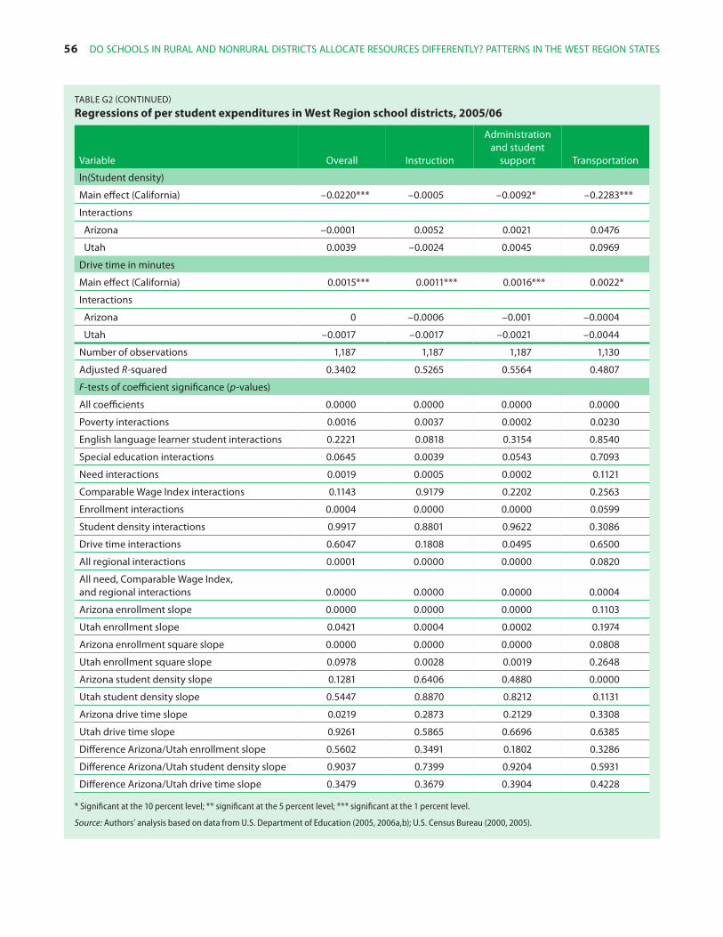
56 do SchoolS in rural and nonrural diSTricTS allocaTe reSourceS differenTly? paTTernS in The WeST region STaTeS
Table g2 (conTinued)
Regressions of per student expenditures in West Region school districts, 2005/06
administration and student
Variable overall instruction support Transportation
ln(Student density)
main effect (california) –0.0220*** –0.0005 –0.0092* –0.2283***
interactions
arizona –0.0001 0.0052 0.0021 0.0476
utah 0.0039 –0.0024 0.0045 0.0969
drive time in minutes
main effect (california) 0.0015*** 0.0011*** 0.0016*** 0.0022*
interactions
arizona 0 –0.0006 –0.001 –0.0004
utah –0.0017 –0.0017 –0.0021 –0.0044
number of observations 1,187 1,187 1,187 1,130
adjusted R-squared 0.3402 0.5265 0.5564 0.4807
F-tests of coefficient significance (p-values)
all coefficients 0.0000 0.0000 0.0000 0.0000
poverty interactions 0.0016 0.0037 0.0002 0.0230
english language learner student interactions 0.2221 0.0818 0.3154 0.8540
Special education interactions 0.0645 0.0039 0.0543 0.7093
need interactions 0.0019 0.0005 0.0002 0.1121
comparable Wage index interactions 0.1143 0.9179 0.2202 0.2563
enrollment interactions 0.0004 0.0000 0.0000 0.0599
Student density interactions 0.9917 0.8801 0.9622 0.3086
drive time interactions 0.6047 0.1808 0.0495 0.6500
all regional interactions 0.0001 0.0000 0.0000 0.0820
all need, comparable Wage index, and regional interactions 0.0000 0.0000 0.0000 0.0004
arizona enrollment slope 0.0000 0.0000 0.0000 0.1103
utah enrollment slope 0.0421 0.0004 0.0002 0.1974
arizona enrollment square slope 0.0000 0.0000 0.0000 0.0808
utah enrollment square slope 0.0978 0.0028 0.0019 0.2648
arizona student density slope 0.1281 0.6406 0.4880 0.0000
utah student density slope 0.5447 0.8870 0.8212 0.1131
arizona drive time slope 0.0219 0.2873 0.2129 0.3308
utah drive time slope 0.9261 0.5865 0.6696 0.6385
difference arizona/utah enrollment slope 0.5602 0.3491 0.1802 0.3286
difference arizona/utah student density slope 0.9037 0.7399 0.9204 0.5931
difference arizona/utah drive time slope 0.3479 0.3679 0.3904 0.4228
* Significant at the 10 percent level; ** significant at the 5 percent level; *** significant at the 1 percent level.
Source: Authors’ analysis based on data from U.S. Department of Education (2005, 2006a,b); U.S. Census Bureau (2000, 2005).

appendix g. regreSSion model reSulTS 57
Table g3
Regressions of staffing ratios in West Region, 2005/06
Variable Teachers administrators
model intercept (reference group is california) 9.1147*** 1.6446***
State-specific controls
arizona 4.7807*** 1.0176***
utah 10.9678* 2.1206*
Student needs
ln(1+poverty)
main effect (california) 0.3216 –0.0272
interactions
arizona 2.1830* 0.2088
utah 7.2037 1.2882
ln(1+ell)
main effect (california) 0.4934* 0.1462**
interactions
arizona –1.5631** –0.0508
utah –0.15 0.582
ln(1+Special education)
main effect (california) 4.9850*** 0.3209*
interactions
arizona –0.8542 0.0766
utah –6.2151 0.1691
Staffing cost
ln(cWi)
main effect (california) –0.3083 0.0247
interactions
arizona –0.9015 –0.2146
utah 1.0537 0.1482
regional characteristics
ln(enrollment)
main effect (california) –0.9718*** –0.2840***
interactions
arizona –1.1550*** –0.2358***
utah –2.2955* –0.4685*
ln(enrollment)2
main effect (california) 0.0479*** 0.0150***
interactions
arizona 0.0728*** 0.0125***
utah 0.1165* 0.0247*
ln(Student density)
main effect (california) –0.0334 –0.0117**
interactions
arizona 0.0006 0.0106
utah –0.0026 –0.0121
(conTinued)
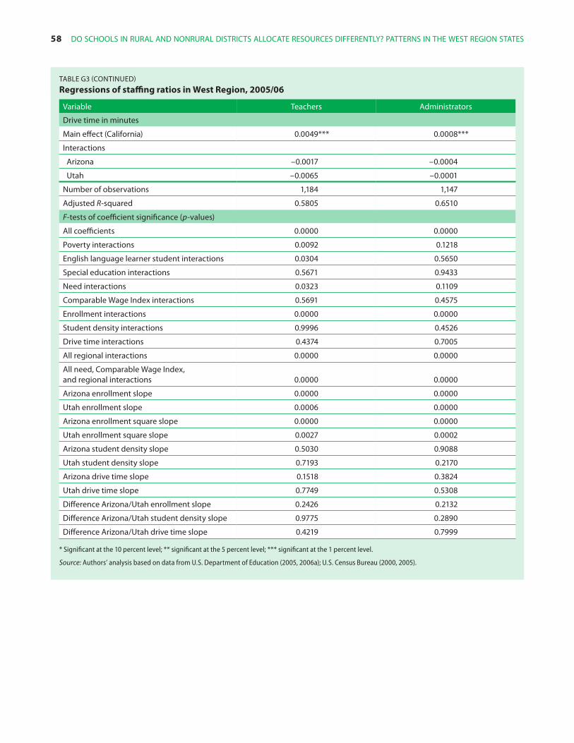
58 do SchoolS in rural and nonrural diSTricTS allocaTe reSourceS differenTly? paTTernS in The WeST region STaTeS
Table g3 (conTinued)
Regressions of staffing ratios in West Region, 2005/06
Variable Teachers administrators
drive time in minutes
main effect (california) 0.0049*** 0.0008***
interactions
arizona –0.0017 –0.0004
utah –0.0065 –0.0001
number of observations 1,184 1,147
adjusted R-squared 0.5805 0.6510
F-tests of coefficient significance (p-values)
all coefficients 0.0000 0.0000
poverty interactions 0.0092 0.1218
english language learner student interactions 0.0304 0.5650
Special education interactions 0.5671 0.9433
need interactions 0.0323 0.1109
comparable Wage index interactions 0.5691 0.4575
enrollment interactions 0.0000 0.0000
Student density interactions 0.9996 0.4526
drive time interactions 0.4374 0.7005
all regional interactions 0.0000 0.0000
all need, comparable Wage index, and regional interactions 0.0000 0.0000
arizona enrollment slope 0.0000 0.0000
utah enrollment slope 0.0006 0.0000
arizona enrollment square slope 0.0000 0.0000
utah enrollment square slope 0.0027 0.0002
arizona student density slope 0.5030 0.9088
utah student density slope 0.7193 0.2170
arizona drive time slope 0.1518 0.3824
utah drive time slope 0.7749 0.5308
difference arizona/utah enrollment slope 0.2426 0.2132
difference arizona/utah student density slope 0.9775 0.2890
difference arizona/utah drive time slope 0.4219 0.7999
* Significant at the 10 percent level; ** significant at the 5 percent level; *** significant at the 1 percent level.
Source: Authors’ analysis based on data from U.S. Department of Education (2005, 2006a); U.S. Census Bureau (2000, 2005).

appendix g. regreSSion model reSulTS 59
Table g4
Regressions of overhead ratios in West Region, 2005/06
Variable Totalcentral
administrationoperations and
maintenance
model intercept (reference group is california) 0.3304*** 0.1955*** 0.1321***
State-specific controls
arizona –0.0585 0.0063 –0.0419
utah 0.0263 –0.0207 0.0503
Student needs
ln(1+poverty)
main effect (california) 0.0231 –0.0156 0.0443*
interactions
arizona 0.2357** 0.0935* 0.1536***
utah –0.198 0.0026 -0.2078
ln(1+ell)
main effect (california) –0.0136 0.0085 –0.0221
interactions
arizona 0.1152* 0.0450 0.043
utah 0.0429 –0.0811 0.1246
ln(1+Special education)
main effect (california) –0.1638** –0.0667 –0.0944**
interactions
arizona 0.3004** 0.1646* 0.0973
utah 0.4173 0.3397 0.0759
Staffing cost
ln(cWi)
main effect (california) 0.0384* 0.0054 0.0337***
interactions
arizona 0.2493** 0.1471** 0.1152**
utah –0.0576 0.0465 –0.1049
regional characteristics
ln(enrollment)
main effect (california) –0.0085*** –0.0116*** 0.0033**
interactions
arizona 0.0042 –0.0053 0.0070*
utah –0.0122 –0.0074 –0.0051
ln(Student density)
main effect (california) –0.0094*** –0.0020* –0.0075***
interactions
arizona –0.0099* –0.0011 –0.0076**
utah 0.0067 0.0061 0.0007
drive time in minutes
main effect (california) 0.0005*** 0.0002** 0.0003***
interactions
arizona –0.0003 –0.0001 –0.0003*
utah –0.0002 0.0000 –0.0003
(conTinued)

60 do SchoolS in rural and nonrural diSTricTS allocaTe reSourceS differenTly? paTTernS in The WeST region STaTeS
Table g4 (conTinued)
Regressions of overhead ratios in West Region, 2005/06
central Variable Total administration
operations and maintenance
number of observations 1,187 1,185 1,187
adjusted R-squared 0.4121 0.3745 0.3651
F-tests of coefficient significance (p-values)
all coefficients 0.0000 0.0000 0.0000
poverty interactions 0.0050 0.1248 0.0005
english language learner student interactions 0.0815 0.3229 0.2478
Special education interactions 0.0146 0.0305 0.2539
need interactions 0.0000 0.0030 0.0000
comparable Wage index interactions 0.0068 0.0107 0.0247
enrollment interactions 0.4459 0.1991 0.0452
Student density interactions 0.0596 0.4903 0.0098
drive time interactions 0.2635 0.8504 0.0497
all regional interactions 0.2393 0.1444 0.0337
all need, comparable Wage index, and regional interactions 0.0000 0.0055 0.0000
arizona enrollment slope 0.3703 0.0000 0.0002
utah enrollment slope 0.1017 0.0153 0.7994
arizona student density slope 0.0000 0.2384 0.0000
utah student density slope 0.7605 0.4512 0.1712
arizona drive time slope 0.4735 0.4580 0.7605
utah drive time slope 0.5681 0.4639 0.8305
difference arizona/utah enrollment slope 0.2287 0.7999 0.1139
difference arizona/utah student density slope 0.0888 0.2345 0.1263
difference arizona/utah drive time slope 0.8265 0.7225 0.9465
* Significant at the 10 percent level; ** significant at the 5 percent level; *** significant at the 1 percent level.
Source: Authors’ analysis based on data from U.S. Department of Education (2005, 2006a,b); U.S. Census Bureau (2000, 2005).
noTeS 61
noTes
1. This study classifies districts into one of seven locale categories: city, suburb, town-not remote, town-remote, rural-fringe, rural-distant, and rural-remote (see explanation of classifications in appendix B). These catego-ries were consolidated into four categories in table 1; greater disaggregation of these data is shown in table 2. See appendix A for counts and percentages of school districts and students for each state broken out by National Center for Education Statistics locale category.
2. Rural districts served 121,715 students in Ari-zona, 299,392 in California, 9,945 in Nevada, and 22,589 in Utah. The tables in appendix A break out the counts and percentages of both districts and students by state and district locale category.
3. Even this figure is an overestimate, as in two of the nine studies “there was no apparent intent to investigate a rural education issue or explain how rurality influences some aspect of schooling” (pp. 2–3).
4. These challenges have been reiterated in the literature for decades. See, for example, Monk, Strike, and Stutz (1981); Walberg and Fowler (1987); Honeyman, Thompson, and Wood (1989); Green and Schneider (1990); Reeves (2003); and Sipple and Brent (2008).
5. The National Center for Education Statistics distinguishes rural from urban locales based on population or proximity to an urban area/
cluster. It defines urbanized areas and clusters as “densely settled cores of census blocks with adjacent densely settled surrounding areas.” When the core contains a population of 50,000 or more it is designated as an urban-ized area. Core areas with populations of 25,000–49,999 are classified as urban clusters (http://nces.ed.gov/ccd/rural_locales.aps).
6. All figures with data on enrollment are limited to districts with a maximum of 6,560 students. All figures with data on student population density are limited to districts with a maximum of 200 students per square mile. All figures with data on drive time to nearest urban area/cluster are limited to dis-tricts that are a maximum of 65 minutes from the nearest urban area/cluster.
7. Nevada was excluded from these multivariate analyses because the small number of school districts (17) in the state made it impossible to reliably estimate model parameters.
8. The transportation expenditure/enrollment patterns for Arizona and Utah were not statis-tically different from those of California.
9. Locale 6 districts are eligible for federal Rural and Low Income Schools grants administered as part of the Rural Education Achievement Program, for example.
10. The descriptive analysis was supplemented with the results of statistical tests (t-tests) of differences in these average measures between nonrural and rural districts (see appendix D).
62 do SchoolS in rural and nonrural diSTricTS allocaTe reSourceS differenTly? paTTernS in The WeST region STaTeS
RefeRences
Arnold, M. L., Biscoe, B., Farmer, T. W., Robertson, D. L., and Shapley, K. L. (2007). How the government defines rural has implications for education policy and practice (Issues & Answers Report, REL 2007-010). Washing-ton, DC: U.S. Department of Education, Institute of Education Sciences, National Center for Education Evaluation and Regional Assistance, Regional Educa-tional Laboratory Southwest.
Arnold, M. L., Newman, J. H., Gaddy, B. B., and Dean, C. B. (2005). A look at the condition of rural educa-tion research: setting a difference for future research. Journal of Research in Rural Education, 20(6). Re-trieved February 20, 2009, from http://jrre.psu.edu/articles/20-6.pdf.
Chambers, J. (1979). School district behavior, markets for educational resources, and the implications for public policy: a survey. In D. Windham (Ed.), Economic dimensions of education. Washington, DC: National Academy of Education.
Chambers, J. (1995). Public school teacher cost differences across the United States: introduction to a Teacher Cost Index (TCI) (NCES 95-758). Washington, DC: U.S. Department of Education, National Center for Educa-tion Statistics.
Collins, T. (1999). Attracting and retaining teachers in rural areas. Charleston, WV: ERIC Clearinghouse on Rural Education and Small Schools. (ERIC ED346082).
Deming, W. E., and Stephan, F. (1941). On the interpreta-tion of censuses as samples. Journal of the American Statistical Association, 36, 45–49.
Duncombe, W., and Yinger, J. (2008). Measurement of cost differentials. In E. Fiske and H.F. Ladd (Eds.), Hand-book of research in education finance and policy. New York: Routledge.
Green, B., and Schneider, M. (1990). Threats to funding for rural schools. Journal of Education Finance, 15(3), 302–318.
Hammer, P., Hughes, G., McClure, C., Reeves, C., and Salgado, D. (2005). Rural teacher recruitment and retention practices: a review of the research literature, national survey of rural superintendents, and case stud-ies of programs in Virginia. Charleston, WV: Appala-chia Educational Laboratory, Inc.
Honeyman, D., Thompson, D., and Wood, C. (1989). Fi-nancing rural and small schools: issues of adequacy and equity. Charleston, WV: ERIC Clearinghouse on Rural Education and Small Schools. (ERIC ED314225).
Imazeki, J., and Rechovsky, A. (2003). Financing adequate education in rural settings. Journal of Education Fi-nance, 29(2), 137–156.
Johnson, J. (2008). New Mexico rural research. In J. Cham-bers (Ed.), An independent comprehensive study of the New Mexico public school funding formula: volume II – technical report. Report prepared for New Mexico State Legislature Funding Formula Study Task Force. Palo Alto, CA: American Institutes for Research.
Johnson, J., and Strange, M. (2009). Why rural matters 2009: state and regional challenges and opportunities. Arling-ton, VA: The Rural School and Community Trust.
Killeen, K., and Sipple, J. (2000). School consolidation and transportation policy: an empirical and institutional analysis. Arlington, VA: Rural School and Community Trust.
Maiden, J., and Stearns, R. (2007). Fiscal equity comparisons between current and capital education expenditures and between rural and nonrural schools in Oklahoma. Journal of Education Finance, 33(2), 147–169.
McLean, J. E., and Ross, S. M. (1994). The urban-rural dis-parity. Charleston, WV: ERIC Clearinghouse on Rural Education and Small Schools. (ERIC ED374957).
McNeil, M. (2009, September 2). Rural areas receive policy tilt. EdWeek, p. 8.
Monk, D., Strike, K., and Stutz, F. (1981). Potential effects of the overburden argument on the funding of rural schools. Report to the New York State Special Task

referenceS 63
Force on Equity and Excellence in Education. Albany, NY: New York State Executive Office.
Parrish, T. B., Matsumoto, C. S., and Fowler, W. Jr. (1995). Disparities in public school district spending, 1989–90 (NCES 95-300). Washington, DC: U.S. Department of Education, National Center for Education Statistics.
Provasnik, S., Kewal-Ramani, A., Coleman, M. M., Gilbert-son, L., Herring, W., and Xie, Q. (2007). Status of edu-cation in rural America (NCES 2007-040). Washington, DC: U.S. Department of Education, National Center for Education Statistics.
Reeves, C. (2003). Implementing the No Child Left Behind Act: implications for rural schools and districts. North Central Regional Educational Lab Report. Retrieved February 20, 2009, from http://www.ncrel.org/policy/pubs/html/implicate/NCLB_PolicyBrief.pdf.
Rural School and Community Trust. (2009). White House rural education meeting identifies key topics. Rural Policy Matters, 11(7), 2.
Sipple, J., and Brent, B. (2008). Challenges and strategies associated with rural school settings. In E. Fiske and H. F. Ladd (Eds.), Handbook of research in education finance and policy. New York: Routledge.
Stern, J. (1994). The condition of education in rural schools. Washington, DC: Office of Educational Research and Im-provement, Programs for the Improvement of Practice.
U.S. Census Bureau. (2000). Cartographic boundary files: 2000 school districts. Washington, DC: U.S. Census Bureau, Geography Division, Cartographic Products Management Branch.
U.S. Census Bureau. (2005). Small Area Income and Poverty Estimates (SAIPE), school district estimates for 2005. Washington, DC: U.S. Census Bureau.
U.S. Department of Education. (2001). Public school finance programs of the United States and Canada: 1998–99 (NCES 2001-309). Washington, DC: U.S. Department of Education, National Center for Education Statistics.
U.S. Department of Education. (2005). 2005 School District Comparable Wage Index (CWI), Version 1a. Wash-ington, DC: U.S. Department of Education, National Center for Education Statistics, Education Finance Statistics Center.
U.S. Department of Education, National Center for Educa-tion Statistics. (2006a). Common Core of Data. Local Education Agency Universe Survey, 2005–06, Version 1a. Retrieved April 27, 2009, from http://nces.ed.gov/ccd/pubagency.asp.
U.S. Department of Education, National Center for Educa-tion Statistics. (2006b). School District Finance Survey (F-33), 2005/06, Version 1a. Retrieved April 27, 2009, from http://nces.ed.gov/ccd/f33agency.asp.
U.S. Department of Education, National Center for Educa-tion Statistics. (2007). Common Core of Data. Local Education Agency Universe Survey, 2005–06, Version 1a. Retrieved April 27, 2009, from http://nces.ed.gov/ccd/pubagency.asp.
Verstegen, D., and Jordan, T. (2009). A fifty-state survey of school finance policies and programs: an overview. Journal of Education Finance, 34, 213–230.
Verstegen, D., Jordan, T., and Amador, P. (2007). A quick glance at school finance: a 50 state survey of school finance policies. Reno, NV: University of Nevada, De-partment of Educational Leadership. Retrieved Febru-ary 20, 2009, from http://wolfweb.unr.edu/homepage/dav3e/SchoolFinanceSurvey2006-07.htm.
Walberg, H., and Fowler, W. (1987). Expenditures and size efficiencies of public school districts. Educational Researcher, 16(7), 5–13.
Walters, D. (1996, March). Rural schools: resource inequali-ties persist. Paper presented at the National Conference on Creating the Quality School, Oklahoma City.
Ward, J. (2003). A case analysis of selected Illinois rural school districts: implications for state rural school finance policy. Journal of Education Finance, 28(4), 599–606.