University of ConnecticutOpenCommons@UConn

Economics Working Papers Department of Economics

July 2008

Do Structural Oil-Market Shocks Affect StockPrices?Nicholas ApergisUniversity of Piraeus

Stephen M. MillerUniversity of Nevada, Las Vegas, and University of Connecticut

Follow this and additional works at: https://opencommons.uconn.edu/econ_wpapers

Recommended CitationApergis, Nicholas and Miller, Stephen M., "Do Structural Oil-Market Shocks Affect Stock Prices?" (2008). Economics Working Papers.200851.https://opencommons.uconn.edu/econ_wpapers/200851

Department of Economics Working Paper Series

Do Structural Oil-Market Shocks Affect Stock Prices?

Nicholas ApergisUniversity of Piraeus

Stephen M. MillerUniversity of Connecticut and University of Nevada, Las Vegas

Working Paper 2008-51R

July 2008

341 Mansfield Road, Unit 1063Storrs, CT 06269–1063Phone: (860) 486–3022Fax: (860) 486–4463http://www.econ.uconn.edu/

This working paper is indexed on RePEc, http://repec.org/

AbstractThis paper investigates how explicit structural shocks that characterize the en-

dogenous character of oil price changes affect stock-market returns in a sample ofeight countries — Australia, Canada, France, Germany, Italy, Japan, the UnitedKingdom, and the United States. For each country, the analysis proceeds in twosteps. First, modifying the procedure of Kilian (2008a), weemploy a vector error-correction or vector autoregressive model to decompose oil-price changes intothree components oil-supply shocks, global aggregate-demand shocks, and globaloil-demand shocks. The last component relates to specific idiosyncratic featuresof the oil market, such as changes in the precautionary demand concerning the un-certainty about the availability of future oil supplies. Second, recovering the oil-supply shocks, global aggregate-demand shocks, and globaloil-demand shocksfrom the first analysis, we then employ a vector autoregressive model to determinethe effects of these structural shocks on the stock market returns in our sample ofeight countries. We find that international stock market returns do not respond ina large way to oil market shocks. That is, the significant effects that exist provesmall in magnitude.

Journal of Economic Literature Classification: G12, Q43

Keywords: real stock returns; structural oil-price shocks; variancedecompo-sition

Do Structural Oil-Price Shocks Affect Stock Prices?

1. Introduction

The existing literature contains several attempts to identify the effects of changes in

international oil prices on certain macroeconomic variables, such as, real GDP growth rates,

inflation, employment, and exchange rates (Hamilton, 1983; Gisser and Goodwin, 1986;

Mork, 1989; Hooker, 1996; Davis and Haltiwanger, 2001, Hamilton and Herrera, 2002, Lee

and Ni, 2002; Hooker, 2002, among others). Their studies differ from each other with respect

to the power of their empirical findings without providing a general consensus.

Fewer research attempts investigate the effects of oil-price changes on asset prices,

such as stock prices or stock returns. Market participants want a framework that identifies

how oil-price changes affect stock prices or stock market returns. On theoretical grounds, oil-

price shocks affect stock market returns or prices through their effect on expected earnings

(Jones et al., 2004). The relevant literature includes the following studies. Kaul and Seyhun

(1990) and Sadorsky (1999) report a negative effect of oil-price volatility on stock prices.

Jones and Kaul (1996) show that international stock prices do react to oil price shocks. Huang

et al. (1999) provide evidence in favor of causality effects from oil futures prices to stock

prices. More recently, Faff and Brailsford (2000) report that oil-price risk proved equally

important to market risk, in the Australian stock market. Hong et al. (2002) also identify a

negative association between oil-price returns and stock-market returns. Pollet (2002) and

Dreisprong et al. (2003) find that oil-price changes predict stock market returns on a global

basis, while Hammoudeh and Li (2004) and Hammoudeh and Eleisa (2004) also discover the

importance of the oil factor for stock prices in certain oil-exporting economies. Bittlingmayer

(2005) documents that oil-price changes associate with war risk and those associated with

other causes exhibit an asymmetric effect on the behavior of stock prices. Sawyer and

2

Nandha (2006), however, using a hierarchical model of stock returns, report results against

the importance of oil prices on aggregate stock returns, while they retain their explanatory

power only on an industrial (sectoral) level. Finally, Gogineni (2007) also provides statistical

support for a number of hypotheses, such as oil prices positively associate with stock prices,

if oil price shocks reflect changes in aggregate demand, but negatively associate with stock

prices, if they reflect changes in supply. Moreover, stock prices respond asymmetrically to

changes in oil prices.

Recently, however, researchers began asking whether changes in macroeconomic

variables cause oil price changes, leading to the decomposition of those oil price changes into

the structural shocks hidden behind such changes (Kilian, 2008a; Kilian and Park, 2007).

That is, different sources of oil price changes may imply non-uniform effects on certain

macroeconomic variables. More specifically, the relevant literature generates mixed views

regarding the effect of such oil-price shocks on asset prices, such as stock prices. Chen et al.

(1986) argue that oil prices do not affect the trend of stock prices, while Jones and Kaul

(1996) present evidence that favors a negative association. This negative relationship,

however, does not receive support by Huang et al. (1996) and Wei (2003).

Kilian (2008a) criticizes all these analyses, because researchers treat oil-price shocks

as exogenous. Certain work, however, argues that oil prices respond to factors that also affect

stock prices (Barsky and Kilian 2002, 2004; Hamilton 2005; Kilian 2008b). Thus, researchers

must decompose aggregate oil price shocks into the structural factors that reflect the

endogenous character of such shocks.

Thus, this paper investigates how the explicit structural shocks characterizing the

endogenous character of oil-price changes affect stock prices across a sample of eight

countries – Australia, Canada, France, Germany, Italy, Japan, the United Kingdom, and the

United States. For each country, the analysis proceeds in two steps. First, modifying the

3

procedure of Kilian (2008a), we employ a vector error-correction or a vector autoregressive

model to decompose oil-price changes into three components: oil-supply shocks, global

aggregate-demand shocks, and global oil-demand shocks. The last component relates to

specific idiosyncratic features of the oil market, such as changes in the precautionary demand

concerning the uncertainty about the availability of future oil supplies. Second, recovering the

oil-supply shocks, global aggregate-demand shocks, and global oil-demand shocks from the

first analysis, we then employ a vector autoregressive model to determine the effects of these

structural shocks on the stock market returns in our sample of eight countries. For

completeness and comparison to Kilian and Park (2007), we also estimate vector

autoregressive models where the changes in the level variables from the oil market replace

the oil-market shocks. The rest of the paper is organized as follows. Section 2 presents the

empirical methodology. Section 3 reports and discusses the empirical results. Finally Section

4 concludes and provides implications of the results as well as suggestions for further

research.

2. Methodology

The proposed methodology considers oil prices as potentially endogenous in an economic

framework. This will enable researchers as well as policy makers to identify explicitly the

exact effects of oil prices changes on certain substantial macroeconomic variables and/or

asset prices, such as stock prices. The methodology uses the vector error-correction (VEC) or

vector autoregressive (VAR) model as appropriate, where we decompose the unpredictable

changes in real oil prices into mutually orthogonal components. Such decompositions carry a

significant economic interpretation and reveal certain implications for both researchers and

policy makers. In particular, the VEC or VAR model contains three variables, global oil

production (OY), global real economic activity (YY), and real oil prices (oil prices deflated by

the CPI index), (ROP). In the VEC model, we also include the error-correction term that

4

emerges because of a long-term cointegrated relationship between these three variables. The

VEC form is given as follows:

- 11

α β δ −=

Δ = + Δ +∑p

t i t i ti

+ tX X EC e

i t

(1)

where X is a 3x1 vector of the variables entering the VER model -- global oil production,

global real economic activity, and real oil prices, Δ is the first-difference operator, EC is the

error-correction term that comes from the cointegrating relationship between the three

variables, and e is a 3x1 vector of residuals from the VEC model. Setting the coefficient of

the error-correction term to zero produces the VAR model as follows:

-1

+α β=

Δ = + Δ∑p

t i ti

X X e

.⎤⎥⎥⎥⎦

(2)

Next, we define ε as the vector of serially and mutually uncorrelated structural

innovations obeying a specific structural pattern, such as:

21

31 32

1 0 01 0

1

OY oil supply shock

YY global demand shock

ROP idiosyncratic demand shock

ee ae a a

εε

ε

−

−

⎡ ⎤ ⎡⎡ ⎤⎢ ⎥ ⎢⎢ ⎥=⎢ ⎥ ⎢⎢ ⎥⎢ ⎥ ⎢⎢ ⎥⎣ ⎦⎣ ⎦ ⎣

(3)

The assumptions that characterize the behavior of the error structure come from Kilian

(2008a) and include the following. First, we assume that global oil production shocks (a

proxy for oil-supply shocks, OSS) do not respond to the other two shocks – global-demand

and idiosyncratic shocks. Second, we assume that global real-activity shocks (a proxy for

global aggregate-demand shocks, GDS) respond to oil-supply shocks, suggesting a sluggish

response of global real economic activity to changes in oil prices. Finally, we assume that

real oil-price shocks (a proxy for idiosyncratic demand shocks, IDS) respond to both oil-

supply and global aggregate-demand shocks, reflecting the importance of fluctuations in

precautionary demand for oil driven by fears concerning the availability of future oil supplies

as well as the importance of certain oil sector-specific policies, such as inventory policies.

5

The exogeneity of the oil-supply shock rests on the grounds that oil production reacts slowly

to changes in demand shocks, a fact mainly attributable to the high costs of oil-production

adjustment and/or to the high uncertainty in the oil market.

Kilian and Park (2007) provide the basic framework for our analysis with some

notable adjustments to their original methodology. To wit, they estimate a structural VAR

model for the four variables as follows: the percentage change in world crude oil production,

global real economic activity, the real oil price, and return on U.S. stocks. As we show below,

the percentage change in world crude oil production and the return on U.S. stocks are

stationary variables (i.e., I(0) variables) whereas global real economic activity and the real

price of oil are non-stationary variables (i.e., I(1) variables). Thus, we argue that Kilian and

Park (2007) estimate a structural VAR model that incorporates variables with inconsistent

time-series properties.

Thus, we modify Kilian’s (2008a) procedure for recovering oil market shocks by

estimating a three variable structural VEC or VAR model, using global oil production (and

not its percentage change), global real economic activity, and the real price of oil. As such,

our three variables prove consistent in a time-series sense, since they all are I(1). Next, we

recover the structural shocks from the three-variable structural VEC or VAR to combine with

the stock market return in a four-variables structural VEC or VAR model. Note that the stock

market return is I(0) as are the three structural shocks. That is, we achieve consistency in the

time-series properties of the variables in our four-variable structural VEC or VAR.

For comparison purposes, we also estimate a four-variable structural VEC or VAR

that comes closer to the specification of Kilian and Park (2007). Here, we use global oil

production (and not its percentage change), global real economic activity, the real price of oil,

and the stock market price (and not its rate of return). Thus, each of the four variables is I(1),

6

once again achieving consistency in the time-series properties of the variables included in the

four-variable VEC or VAR.

3. Empirical Analysis

3.1 Data

We collect monthly data on goods prices (P) proxied by the consumer price index (CPI),

global real economic activity proxied by a global index of dry cargo single voyage freight

rates,1 the international oil price (OP) proxied by the US price per barrel of crude oil, oil

production proxied by the US price per barrel of crude oil, and stock market price (SP) in

each country. Kilian (2008a) argues for the validity of the dry-cargo single-voyage freight

rates as a proxy for global economic activity on the grounds that these rates rise and fall with

rises and falls in global demand. That is, rising global demand leads to rising trade and rising

demand for shipping services. Consequently, rising global demand should associate with

rising freight rates. The proxy for world demand sidesteps a sticky issue with individual

country data. To wit, researchers typically approximate global demand with some weighted

average of the larger individual country demands. The index of freight weights potentially

captures changes in total world demand, including the smaller countries omitted by those

indexes that use aggregates of individual country data.

The monthly sample for the eight countries -- Australia, Canada, France, Germany,

Italy, Japan, the United Kingdom, and the United States – spans 1981 to 2007 inclusive for a

total of 324 observations for each country. Data on consumer price indices and oil prices

come from the International Financial Statistics (IFS) database, while stock market prices

come from Datastream.2

1 Kilian provides his proxy for global real economic activity on his website at http://www-personal.umich.edu/~lkilian/paperlinks.html. 2 Stock market prices reflect the following markets: Australia by the Australian General Market Index, Canada by the C.L. Toronto Index, Germany by the DAX index, France by the CAC Industrial Index, Italy by the Milan

7

For our empirical analysis, we deflate oil prices as well as stock prices by goods

prices (i.e., the respective CPI). Next, we compute stock returns as differences in the natural

logarithm of real stock market prices. We employ RATS software (version 7.0) in the

empirical analysis.

3.2 Unit Root Tests

We test for unit roots in the natural logarithms of our variables for each country. We test the

null hypothesis of non-stationary variables versus the alternative hypothesis of stationary

variables using the Augmented Dickey-Fuller (ADF) statistic (Dickey and Fuller, 1981). We

employ the Akaike information criteria (AIC) to select the lag length from the ADF test.

Table 1 reports the results with and without a trend. With one exception, we cannot reject the

null hypothesis that all variables contain a unit root at the 5-percent significant level,

suggesting that the natural logarithm of all variables in our study are I(1). For the exception,

global oil production, we cannot reject the null hypothesis of a unit root at the 1-percent level.

3.3 Cointegration Tests

We employ cointegration tests, based on the methodology of Johansen and Juselius (1990),

for the variables that characterize the global oil market -- global oil production, global real

economic activity, and real oil prices. Table 2 reports the tests for cointegration. As a pre-test,

we estimate VAR models with varying lag lengths and perform F-tests to select the

appropriate lag length. In all cases, we choose seven lags.3 Both the eigenvalue and the trace

test statistics recommend that a long-run relationship does not exist among the three jointly

determined variables in either case.4

IB 30 index, Japan by the Nikkei Stock Index, the United Kingdom by the Financial Times 30 index, and the United States by the NYSE index. 3 Since two variables are identical across the countries and the third variable is the real oil price in each country, we do not anticipate that the results will differ dramatically across countries. Thus, finding the same lag length in each country does not raise concerns. 4 Thus, since we do not employ cointegration, our finding that the log-level of oil supply does not contain a unit root does not create any problems.

8

Thus, we proceed to estimate VAR models for all eight countries. Since two of the

variables – global oil production and global real economic activity – do not change across the

eight different specifications, we do not expect dramatic differences in results. That is, only

the real oil price differs across countries due to different CPI deflators used to generate the

real oil price in each country.

3.4 Variance Decomposition Tests

Table 3 reports the variance decompositions results for the effects of various oil-price shocks

involved in the VAR model only on the real price of oil (ROP) to conserve space. All VAR

models include seven lags. The numbers reported indicate the percentage of the forecast error

in each variable that we can attribute to each of the structural innovations at different

horizons (from 1 month to 60 months). We report the percentages for selected forecast

horizons (1, 6, 12, 36, 60 months).

The decomposition results show that even in the long-run (i.e., the 60-month forecast

horizon), global aggregate-demand shocks contribute a relatively small share to the variation

in real oil prices. In the short run (i.e., 1-month forecast horizon), oil-supply and global-

demand shocks produce slightly less than 3-percent of the variation in the real price of oil

across all eight countries in our sample. Extending the focus to the long-run (i.e., 60-month

forecast horizon, the oil-supply and global-demand shocks only generate between 7- and 8-

percent of the variation of real oil price variation. In addition, the speed with which the

variance decomposition reaches its long-run equilibrium occurs rather quickly, falling within

the range of 22 to 32 months for all countries.

In sum, while the variance decompositions show that oil-supply and global-demand

shocks frequently exhibit significant effects on the real oil-price shock, these effects proves

small in magnitude. Moreover, the long-run equilibrium decomposition occurs within a short

time horizon of between 22 to 32 months.

9

3.5 Structural Oil Price Shocks and Stock Returns

This section investigates how the structural oil price innovations relate to asset prices, such as

stock returns (r), where stock-market return equals the difference in natural logarithms of the

stock-market index. That is, we recover the structural shocks from the three-variable VAR

model and combine them with the stock-market return to produce a 4-varaible model.

We, once again, test the null hypothesis of non-stationary variables versus the

alternative hypothesis of stationary variables using the Augmented Dickey-Fuller (ADF)

statistic (Dickey and Fuller, 1981). Table 1 reports the unit-root tests for the three structural

shocks and the stock-market returns, indicating that we can reject the null hypothesis of a unit

root in each case. As before, the AIC statistic determines the lag length on the ADF test. That

is, these four variables prove stationary. Thus, we employ a four-variable VAR model,

involving the stock-market returns and the three structural shocks. We do not need to

consider cointegration, in this case. In addition, each VAR model incorporates seven lags.

Table 4 reports the variance decompositions results for the effects of each of the three

structural oil shocks plus the stock-market returns shocks only on stock-market returns (to

conserve space). The numbers reported, again, indicate the percentage of the forecast error in

each variable that we can attribute to each of the innovations at different horizons (from 1

month to 60 months). We report the percentages for selected forecast horizons (1, 6, 12, 36,

60 months). Moreover, we also observe, once again, that the decompositions reach a long-run

equilibrium rapidly, ranging from 15 to 22 months.

The decomposition results uncover a pattern for the three structural oil shocks. All

three oil-market shocks contribute little to the variation in the stock market returns in each

country. Italy provides the case where oil-market shocks generate the largest effect on the

variation of the stock market return – less than 17-percent. For the remaining seven countries,

the total effect of the oil-market shocks on explaining the variation of stock-market returns

10

range from a low of 7.78 percent to a high of 12.12 percent. Although oil-market shocks

frequently exhibit significant effects on the variation in the stock-market return, these effects

prove, once again, small in magnitude. The results suggest that oil-market shocks exert a

minor influence on stock market returns.

For comparison purposes, we also performed tests on a 4-variable VAR system –

global oil production, global real economic activity, the real oil price, and the real stock

market price. These VAR models capture the spirit of Kilian and Park (2007), but ensure that

the variables employed exhibit the same time series properties (i.e., each variable proves

integrated of order one).5 As noted in the text, Kilian and Park (2007) use the percentage

change in global oil production and the real stock return, both of which prove stationary in

our analysis, along with global real economic activity and the real oil price. In other words,

Kilian and Park (2007) appear to use two I(1) and two I(0) variables in their VAR system.

The results of our 4-variabeles VAR model produces findings consistent to those reported in

the text. Results of these alternative 4-variabel VAR models are available on request.

Kilian and Park (2007) report results form the United States with, as just described, a

slightly different specification. Our findings do not differ dramatically from theirs. They find

a slightly smaller effect of oil market shocks on the stock market return in the short run and a

significantly higher effect in the longer run, where the three shocks explain around 11 percent

at 12 months and just over 22 percent at infinity. We explain just over 12 percent after 12

months, and this does not change through 60 months. In addition, they report results that

continue to increase the percentage of the stock-market return explained over time, although

not by much. Our findings reach long-run equilibrium after 22 months.

Finally, we consider the potential temporal causality of our three oil-market shocks on

the stock market returns in the eight countries in our sample. Table 5 reports the results of

5 We impose the assumption that the log level of oil supply does contain a unit root.

11

Granger temporal causality tests. We find a consistent pattern for four countries – Germany,

Italy, the United Kingdom, and the United States. To wit, the real oil price shock temporally

causes the stock market return at the 5-percent level or better. In Australia’s case, only oil

supply shocks temporally cause the stock market return, whereas in France’s case, only

global aggregate demand shocks temporarily lead the stock-market return. For Canada and

Japan, we uncover no causality effects. Finally, we find no temporal causality of the oil-

market shocks on the stock-market return.

4. Conclusions, Implications, and Suggestions for Further Research

Our paper provides the first multi-country examination of the effects of oil-market shocks on

stock markets. This study includes a sample of eight countries, – Australia, Canada, France,

Germany, Italy, Japan, the United Kingdom, and the United States. Using the methodology of

Kilian (2008a), we compute three different structural shocks for the oil market that captures

oil supply shocks, global aggregate-demand shocks, and idiosyncratic demand shocks.

Recovering the three structural shocks from the first-stage calculation, we combine those

shocks with the stock-market returns to consider how the oil market structural shocks affect

the evolution of the stock market returns.

The results show that different oil-market structural shocks play a significant role in

explaining the adjustments in stock-market returns. But, the magnitude of such effects proves

small. More specifically, oil-supply shocks, aggregate global-demand shocks, and oil-market

idiosyncratic demand shocks all contribute significantly to explaining stock-market returns in

most countries from the variance decompositions. The oil-supply and global aggregate-

demand shocks do not significantly explain the stock return in Australia, whereas the

idiosyncratic demand shocks affect the stock return in Canada at a weaker level of

significance. Further, the Granger temporal causality tests suggest a strong role for

12

idiosyncratic demand shocks leading the stock market returns, whereas the oil-supply and

global aggregate-demand shocks do not as a rule temporally lead the stock-market return.

Future research efforts could also investigate the effect of such structural oil-market

shocks on real stock returns across manufacturing industries for a panel of countries. The

empirical findings will prove extremely useful to investors who need to understand the exact

effect of international oil price changes on certain stocks across industries.

13

References

Barsky, R. B. and Kilian, L. (2004) “Oil and the Macroeconomy since the 1970s., Journal of

Economic Perspectives 18, 115-134.

Barsky, R. B. and Kilian, L. (2002) “Do we Really Know that Oil Caused the Great

Stagflation? A Monetary Alternative.” NBER Macroeconomics Annual 2001, 137-

183.

Bittlingmayer, G. (2005) “Oil and Stocks: Is it War Risk?” Working Paper Series, University

of Kansas.

Chen, N. F., Roll, R. and Ross, S. A. (1986) “Economic Forces and the Stock Market.”

Journal of Business 59, 383-403.

Davis, J. S. and Haltiwanger, J. (2001) “Sectoral Job Creation and Destruction Responses to

Oil Price Changes.” Journal of Monetary Economics 48, 465-512.

Dickey, D.A. and Fuller, W.A. (1981) “Likelihood Ratio Statistics for Autoregressive Time

Series With a Unit Root.” Econometrica 49, 1057-1072.

Driesprong, G., Jacobsen, B. and Benjiman, M. (2003) “Striking Oil: Another Puzzle?”

Working Paper, Erasmus University Rotterdam.

Faff, R. W. and Brailsford, T. J. (2000) “A Test of a Two-Factor ‘Market and Oil’ Pricing

Model.” Pacific Accounting Review 12, 61-77.

Gisser, M. and Goodwin, T. H. (1986) “Crude Oil and the Macroeconomy: Tests of Some

Popular Notions: Note.” Journal of Money, Credit and Banking 18, 95-103.

Gogineni, S. (2007) “The Stock Market Reaction to Oil Price Changes.” Working Paper,

University of Oklahoma.

Hamilton, J. D. (2005) “Oil and the Macroeconomy.” in S. Durlauf and L. Blume (eds.), The

New Palgrave Dictionary of Economics, 2nd Edition, London: Macmillan.

Hamilton, J. D. (2003) “What is an Oil Shock?” Journal of Econometrics 113, 363-398.

14

Hamilton, J. D. (1983) “Oil and the Macroeconomy since World War II.” The Journal of

Political Economy 9, 228-248.

Hamilton, J. D. and Herrera, M. A. (2002) “Oil Shocks and Aggregate Macroeconomic

Behavior.” Journal of Money, Credit and Banking 36, 265-286.

Hammoudeh, S. and Li, H. (2004) “Risk-Return Relationships in Oil-Sensitive Stock

Markets.” Finance Letters 2, 10-15.

Hammoudeh, S. and Eleisa, E. (2004) “Dynamic Relationships among the GCC Stock

Markets and the NYMEX Oil Prices.” Contemporary Economic Policies 22, 250-269.

Hong, H., Torous, W. and Valkanov, R. (2002) “Do Industries lead the Stock Market?

Gradual Diffusion of Information and Cross-Asset Return Predictability.” Working

Paper, Stanford University and UCLA.

Hooker, M. A. (2002) “Are Oil Shocks Inflationary? Asymmetric and Nonlinear

Specifications versus Changes in Regime.” Journal of Money, Credit and Banking 34,

540-561.

Hooker, M. A. (1996) “What Happened to the Oil-Price Macroeconomy Relationship?”

Journal of Monetary Economics 38, 195-213.

Huang, R., Masulis, R. and Stoll, H. (1996) “Energy Shocks and Financial Markets.” Journal

of Futures Markets 16, 1-17.

Im, K. S., Pesaran, M. H., and Shin Y. (1995) “Testing for Unit Roots in Heterogeneous

Panels.” Working Paper 9526, Department of Applied Economics, Cambridge

University.

Jones, D. W., Lelby, P. N. and Paik, I. K. (2004) “Oil Price Shocks and the Macroeconomy:

What Has Been Learned Since 1996?” Energy Journal 25, 1-32.

Jones, C. and Kaul, G. (1996) “Oil and the Stock Markets.” Journal of Finance 51, 463-491.

15

Kaul, G. and Seyhun, N. (1990) “Relative Price Variability, Real Shocks, and the Stock

Market.” The Journal of Finance 45, 479-496.

Kilian, L. (2008a) “Not All Oil Price Shocks are Alike: Disentangling Demand and Supply

Shocks in the Crude Oil Market.” American Economic Review in press.

Kilian, L. (2008b) “Exogenous Oil Supply Shocks: How Big Are They and How Much do

they Matter for the US Economy?” Review of Economics and Statistics 90. 216-240

Kilian, L. and Park, C. (2007) “The Impact of Oil Price Shocks on the U.S. Stock Market.”

CPER Discussion Paper 6166.

Lee, K. and Ni, S. (2002) “On the Dynamic Effects of Oil Shocks: A Study Using Industry

Level Data.” Journal of Monetary Economics 49, 823-852.

Mork, A. K. (1989) “Oil and the Macroeconomy when Prices Go Up and Down: An

Extension of Hamilton’s Results.” The Journal of Political Economy 97, 740-744.

Pedroni, P. (1999) “Critical Values for Cointegration Tests in Heterogeneous Panels with

Multiple Regressors.” Oxford Bulletin of Economics and Statistics 61, Special Issue,

653-670.

Pollet, J. (2002) “Predicting Asset Returns with Expected Oil Price Changes.” Working

Paper, Harvard University.

Sadorsky, P. (1999) “Oil Price Shocks and Stock Market Activity.” Energy Economics 2,

449-469.

Sawyer, K. R. and Nandha, M. (2006) “How Oil Moves Stock Prices.” Working Paper Series,

University of Melbourne.

Wei, C. (2003) “Energy, the Stock Market, and the Putty-Clay Investment Model.” American

Economic Review 93, 311-323.

16

Table 1: Unit-Root Tests

Variables Without Trend With Trend Without Trend With Trend Levels First Differences

OY -0.32(12) -4.13(12)*** -5.91(12)*** -5.88(12)*** YY -1.01(12) -2.61(12) -3.85(12)*** -3.88(12)**

Australia ROP -1.97(11) -1.42(12) -5.17(12)*** -5.59(12)*** r -5.89(12)*** -5.86(12)*** εOSS -5.35(11)*** -5.34(11)*** εGDS -3.72(12)*** -3.72(12)**

εIDS -4.42(12)*** -4.88(12)***

Canada ROP -1.70(11) -1.40(12) -5.19(12)*** -5.58(12)*** r -5.98(12)*** -5.94(12)*** εOSS -5.36(11)*** -5.35(11)*** εGDS -3.73(12)*** -3.72(12)**

εIDS -4.51(12)*** -4.88(12)***

France ROP -1.55(11) -1.43(12) -5.24(12)*** -5.52(12)*** r -4.85(9)*** -4.86(9)*** εOSS -5.37(11)*** -5.36(11)*** εGDS -3.73(12)*** -3172(12)**

εIDS -4.46(12)*** -4.95(12)***

Germany ROP -1.66(114) -1.47(12) -5.21(12)*** -5.58(12)*** r -5.08(9)*** -5.15(9)*** εOSS -5.37(11)*** -5.36(11)*** εGDS -3.72(12)*** -3.71(12)***

εIDS -4.53(12)*** -4.93(12)***

Italy ROP -2.04(11) -1.32(12) -5.11(12)*** -5.60(12)*** r -3.44(12)** -3.49(12)** εOSS -5.36(11)*** -5.36(11)*** εGDS -3.73(12)*** -3.72(12)**

εIDS -4.38(12)*** -4.94(12)***

Japan ROP -0.91(12) -1.36(12) -5.24(12)*** -5.59(12)*** r -6.93(4)*** -5.36(8)*** εOSS -5.12(11)*** -5.34(11)*** εGDS -3.73(12)*** -3.72(12)**

εIDS -4.54(12)*** -4.98(12)***

17

Table 1: Unit-Root Tests (continued)

Variables Without Trend With Trend Without Trend With Trend Levels First Differences United Kingdom

ROP -1.71(11) -1.29(12) -5.18(12)*** -5.58(12)*** r -5.12(9)*** -5.91(9)*** εOSS -5.58(11)*** -5.36(11)*** εGDS -3.73(12)*** -3.72(12)**

εIDS -4.47(12)*** -4.96(12)***

United States ROP -1.80(11) -1.40(12) -5.22(12)*** -5.55(12)*** r -3.88(4)** -4.78(11)*** εOSS -5.36(11)*** -5.34(11)*** εGDS -3.72(12)*** -3.72(12)**

εIDS -4.53(12)*** -4.96(12)*** ___________________________________________________________________________ Note: OY is the log of global oil production, YY is the log of real economic activity, ROP is the log

of real oil prices, r is stock returns, εOSS is the structural oil supply shock, εGDS is the structural global demand shock, and εIDS is the structural idiosyncratic demand shock. Figures in brackets denote the number of lags in the augmented term that ensures white-noise residuals. We determined the optimal lag length through the Akaike information Criterion (AIC) and the Schwarz-Bayes Information Criterion (SBIC), whose critical values equal the following values: 1-percent = -3.45, 5-percent = -2.87, 10-percent = -2.56.

*** Significant at 1%. ** Significant at 5%.

18

Table 2: Cointegration Tests

r n-r m.λ. 95% Tr 95% Australia (Lags=7)

r=0 r=1 19.1125 25.8100 31.0784 35.0700 r<=1 r=2 7.2184 11.4600 11.9609 20.1600

r<=2 r=3 4.7425 9.1400 4.7425 9.1400 Canada (Lags=7)

r=0 r=1 19.3595 25.8100 30.5154 35.0700 r<=1 r=2 6.2921 11.4600 11.1560 20.1600

r<=2 r=3 4.8639 9.1400 4.8639 9.1400 France (Lags=7)

r=0 r=1 19.8392 25.8100 31.3614 35.0700 r<=1 r=2 6.5962 11.4600 11.5222 20.1600

r<=2 r=3 4.8260 9.1400 4.8260 9.1400 Germany (Lags=7)

r=0 r=1 19.4305 25.8100 29.9744 35.0700 r<=1 r=2 5.5501 11.4600 10.5439 20.1600

r<=2 r=3 4.9938 9.1400 4.9938 9.1400 Italy (Lags=7)

r=0 r=1 20.1190 25.8100 32.8336 35.0700 r<=1 r=2 7.9983 11.4600 12.7146 20.1600

r<=2 r=3 4.7163 9.1400 4.7164 9.1400 Japan (Lags=7)

r=0 r=1 19.2739 25.8100 30.1623 35.0700 r<=1 r=2 5.3234 11.4600 10.8284 20.1600

r<=2 r=3 5.3052 9.1400 5.3052 9.1400 United Kingdom (Lags=7)

r=0 r=1 18.7061 25.8100 30.0768 35.0700 r<=1 r=2 6.4261 11.4600 11.3707 20.1600

r<=2 r=3 4.9445 9.1400 4.9445 9.1400 United States (Lags=7)

r=0 r=1 18.9051 25.8100 29.6546 35.0700 r<=1 r=2 5.9236 11.4600 10.7495 20.1600 r<=2 r=3 4.8258 9.1400 4.8258 9.1400

Note: r = number of cointegrating vectors, n-r = number of common trends, m.λ.= maximum eigenvalue

statistic, Tr = trace statistic.

19

Table 3: Variance Decomposition Tests (Oil Shocks)

Real Oil Price (ROP)

Months OY YY ROP

Australia (27) 1 0.22 2.55 97.23 (?.??) (?.??) (?.??) 6 2.38 4.20 93.42 (?.??) (?.??) (?.??) 12 3.16 4.43 92.41 (?.??) (?.??) (?.??) 36 3.21 4.43 92.36 (?.??) (?.??) (?.??) 60 3.21 4.43 92.36 (?.??) (?.??) (?.??)

Canada (23) 1 0.21 2.71 97.09 (?.??) (?.??) (?.??) 6 2.30 4.41 93.30 (?.??) (?.??) (?.??) 12 3.08 4.63 92.29 (?.??) (?.??) (?.??) 36 3.13 4.63 92.23 (?.??) (?.??) (?.??) 60 3.13 4.63 92.23 (?.??) (?.??) (?.??)

France (22) 1 0.17 2.61 97.23 (?.??) (?.??) (?.??) 6 2.23 4.27 93.51 (?.??) (?.??) (?.??) 12 2.99 4.51 92.50 (?.??) (?.??) (?.??) 36 3.03 4.51 92.45 (?.??) (?.??) (?.??) 60 3.03 4.51 92.45 (?.??) (?.??) (?.??)

Germany (28) 1 0.18 2.75 97.23 (?.??) (?.??) (?.??) 6 2.52 4.52 93.16 (?.??) (?.??) (?.??) 12 3.14 4.72 92.13 (?.??) (?.??) (?.??) 36 3.19 4.23 92.08 (?.??) (?.??) (?.??) 60 3.19 4.23 92.08 (?.??) (?.??) (?.??)

20

Table 3: Variance Decomposition Tests (Oil Shocks) (continued)

Real Oil Price (ROP)

Months OY YY ROP

Italy (28) 1 0.21 2.60 97.20 (?.??) (?.??) (?.??) 6 2.41 4.14 93.34 (?.??) (?.??) (?.??) 12 3.17 4.48 92.35 (?.??) (?.??) (?.??) 36 3.21 4.48 92.31 (?.??) (?.??) (?.??) 60 3.21 4.48 92.31 (?.??) (?.??) (?.??)

Japan (22) 1 0.18 2.61 92.21 (?.??) (?.??) (?.??) 6 2.19 4.19 93.62 (?.??) (?.??) (?.??) 12 2.93 4.42 92.65 (?.??) (?.??) (?.??) 36 2.98 4.43 92.60 (?.??) (?.??) (?.??) 60 2.98 4.43 92.60 (?.??) (?.??) (?.??)

United Kingdom (32) 1 0.13 2.66 97.21 (?.??) (?.??) (?.??) 6 2.18 4.53 93.49 (?.??) (?.??) (?.??) 12 3.04 4.59 92.37 (?.??) (?.??) (?.??) 36 3.08 4.60 92.32 (?.??) (?.??) (?.??) 60 3.08 4.60 92.32 (?.??) (?.??) (?.??)

United States (27) 1 0.21 2.65 97.14 (?.??) (?.??) (?.??) 6 2.32 4.32 93.36 (?.??) (?.??) (?.??) 12 3.14 4.55 92.31 (?.??) (?.??) (?.??) 36 3.19 4.56 92.26 (?.??) (?.??) (?.??) 60 3.19 4.56 92.26 (?.??) (?.??) (?.??)

21

Table 3: Variance Decomposition Tests (Oil Shocks) (continued)

Notes: Standard errors, estimated through Monte Carlo techniques and 1000 replications, appear in

parentheses under percentage of variances explained. The numbers in parentheses after the country name represent the number of periods until the variance decomposition reaches a constant, unchanging value for all future periods.

22

Table 4: Variance Decomposition Tests (Real Stock Return)

Stocks Returns (r)

Months εOSS εGDS εIDS r

Australia (19) 1 1.16 0.02 0.39 98.44 (?.??) (?.??) (?.??) (?.??) 6 3.17 2.69 3.20 90.94 (?.??) (?.??) (?.??) (?.??) 12 4.29 2.95 3.68 89.10 (?.??) (?.??) (?.??) (?.??) 36 4.31 2.97 3.68 89.05 (?.??) (?.??) (?.??) (?.??) 60 4.31 2.97 3.68 89.05 (?.??) (?.??) (?.??) (?.??)

Canada (20) 1 1.45 0.72 0.61 97.22 (?.??) (?.??) (?.??) (?.??) 6 2.06 1.87 1.81 91.97 (?.??) (?.??) (?.??) (?.??) 12 3.23 2.01 2.53 92.24 (?.??) (?.??) (?.??) (?.??) 36 3.24 2.01 2.53 92.22 (?.??) (?.??) (?.??) (?.??) 60 3.24 2.01 2.53 92.22 (?.??) (?.??) (?.??) (?.??)

France (15) 1 0.77 0.67 0.45 98.12 (?.??) (?.??) (?.??) (?.??) 6 2.50 3.39 4.34 89.77 (?.??) (?.??) (?.??) (?.??) 12 2.71 4.60 4.43 88.26 (?.??) (?.??) (?.??) (?.??) 36 2.72 4.60 4.43 88.25 (?.??) (?.??) (?.??) (?.??) 60 2.72 4.60 4.43 88.25 (?.??) (?.??) (?.??) (?.??)

Germany (21) 1 0.38 0.33 0.09 99.21 (?.??) (?.??) (?.??) (?.??) 6 1.08 2.02 5.50 91.40 (?.??) (?.??) (?.??) (?.??) 12 2.07 2.23 5.92 89.79 (?.??) (?.??) (?.??) (?.??) 36 2.09 2.23 5.92 89.77 (?.??) (?.??) (?.??) (?.??) 60 2.09 2.23 5.92 89.77 (?.??) (?.??) (?.??) (?.??)

23

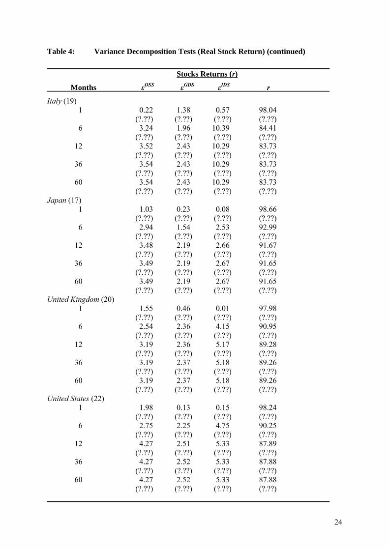
Table 4: Variance Decomposition Tests (Real Stock Return) (continued)

Stocks Returns (r)

Months εOSS εGDS εIDS r

Italy (19) 1 0.22 1.38 0.57 98.04 (?.??) (?.??) (?.??) (?.??) 6 3.24 1.96 10.39 84.41 (?.??) (?.??) (?.??) (?.??) 12 3.52 2.43 10.29 83.73 (?.??) (?.??) (?.??) (?.??) 36 3.54 2.43 10.29 83.73 (?.??) (?.??) (?.??) (?.??) 60 3.54 2.43 10.29 83.73 (?.??) (?.??) (?.??) (?.??)

Japan (17) 1 1.03 0.23 0.08 98.66 (?.??) (?.??) (?.??) (?.??) 6 2.94 1.54 2.53 92.99 (?.??) (?.??) (?.??) (?.??) 12 3.48 2.19 2.66 91.67 (?.??) (?.??) (?.??) (?.??) 36 3.49 2.19 2.67 91.65 (?.??) (?.??) (?.??) (?.??) 60 3.49 2.19 2.67 91.65 (?.??) (?.??) (?.??) (?.??)

United Kingdom (20) 1 1.55 0.46 0.01 97.98 (?.??) (?.??) (?.??) (?.??) 6 2.54 2.36 4.15 90.95 (?.??) (?.??) (?.??) (?.??) 12 3.19 2.36 5.17 89.28 (?.??) (?.??) (?.??) (?.??) 36 3.19 2.37 5.18 89.26 (?.??) (?.??) (?.??) (?.??) 60 3.19 2.37 5.18 89.26 (?.??) (?.??) (?.??) (?.??)

United States (22) 1 1.98 0.13 0.15 98.24 (?.??) (?.??) (?.??) (?.??) 6 2.75 2.25 4.75 90.25 (?.??) (?.??) (?.??) (?.??) 12 4.27 2.51 5.33 87.89 (?.??) (?.??) (?.??) (?.??) 36 4.27 2.52 5.33 87.88 (?.??) (?.??) (?.??) (?.??) 60 4.27 2.52 5.33 87.88 (?.??) (?.??) (?.??) (?.??)

24

Table 4: Variance Decomposition Tests (Real Stock Return) (continued)

Notes: See Table 3. Once again, the numbers in parentheses after the country name represents the

number of periods until the variance decomposition reaches a constant, unchanging value for all future periods.

25

26

Table 5: Temporal Causality Tests (Real Stock Return)

Stocks Returns (r) Temporally Caused by

εOSS εGDS εIDS

Australia 1.75* 1.50 1.59 Canada 0.80 0.46 0.86 France 0.84 1.89* 1.58 Germany 0.87 0.97 2.66** Italy 1.66 0.60 4.67*** Japan 1.39 0.73 1.07 United Kingdom 0.84 0.90 2.49** United States 1.36 1.07 2.52** Notes: The test statistics are F-tests of the hypothesis that the lagged shocks do not significantly

explain the stock-market return. *** Significant at 1-percent level. ** Significant at 5-percent level. * Significant at 10-percent level.