doctor of philosophy - shodhgangashodhganga.inflibnet.ac.in/bitstream/10603/26741/1/final...bhabi...
TRANSCRIPT
“Some Relativistic Phenomenain Astrophysics”
THE THESIS SUBMITTED TO
KUMAUN UNIVERSITY, NAINITALFOR THE AWARD OF DEGREE OF
DOCTOR OF PHILOSOPHY
IN
(PHYSICS)BY
PRATIBHA FULORIAUNDER THE SUPERVISION
OF
Supervisor Co-supervisor
Prof. B. C. Joshi Dr. B. C. TewariDepartment OF PHYSICS Department of Mathematics
Kumaun University Kumaun UniversityS. S. J. Campus, Almora S. S. J. Campus, Almora
Uttarakhand Uttarakhand
2012


Acknowledgements
It is a great honour to express my deep sense of gratitude and indebtedness to my
supervisor Prof. B. C. Joshi, Department of Physics, S. S. J. Campus Almora , Kumaun
University , Nainital who gave me an opportunity to work under his kind guidance-ship. I
sincerely thank Dr. B. C. Tiwari, Department of Mathematics, S. S. J. Campus Almora for his
valuable help and direct involvement in the study. His guidance helped me in all the time of
research and encouraged me to complete my thesis work.
I am profoundly indebted to Prof. M. C. Durgapal , Head of Physics Department, S.
S. J. campus Almora, Kumaun University, Nainital for his continuous support and
precious guidance during the progress of my work. I take this opportunity to express my
sincere gratitude and appreciation to Prof. K. L. Sah (Retd.), Prof. O. P. S. Negi, Dr. P. S.
Bisht for their time to time cooperation, invaluable advices and help rendered to me during
the entire period of this work. I now avail this opportunity to extend my grateful thanks to
Pushpa, Gaurav, Bhupesh, Pawan, chauhan, vishal for all possible support rendered to me
during this period.
I also acknowledge time to time cooperation from the members of non - teaching staff
of Physics Department, Soban Singh Jeena Campus, Almora Bhuwan Negi ji, R. S. Rayal ji,
J. C. Upadhayay ji, Heera Singh Kharayat ji, Pramod Nailwal ji, Rajendra Singh Rana ji ,
Bheem Singh ji and Dan Singh ji. In particular, I am grateful to Dr. Santosh, Dr. Ashok for
providing me the research papers and books whenever I was in the urgent need of them
I wish to express my profound gratitude to Late Prof. Mahesh Chandra Durgapal for
enlightening me the first glance of research. His motivation, enthusiasm, and immense
knowledge paved the way for the completion of this difficult task.
iv
I also take this opportunity to express my gratitude to Prof. Kavita Pandey, formerly
Head of Physics Department, Kumaun University, D.S. B. Campus, Nainital for her
inspiration and moral support given to me in many ways. My sincere thanks also go to Dr
Neeraj Pant (Associate Professor) Maths Department, N.D.A., Khadakwasla, Pune for his
stimulating discussions and constructive suggestions during the progress of this work. His
time to time discussions of research problems motivated me to do more and more work. I am
also thankful to Dr. P. S. Negi, Physics Department, D. S. B. Campus, Nainital, Kumaun
University for his guidance and support given to me during this period.
I am deeply indebted to my husband Dr. C. P. Fuloria for his indistinctly help
persistent encouragement and affectionate cooperation, which made it possible to
complete this difficult task. I can not forget the affection and love of my child Dear
Chetan which always enforced me to complete my work without any tension.
It is a pleasure to convey my deep sense of gratitude to my brother Sri Rajesh Joshi,
Bhabi Smt. Anandi Joshi for perpetual inspiration, motivation and invaluable help
given to me whenever I was in the difficult moments. I now avail this opportunity to
express my thanks to my elder sisters Pushpa didi, Geeta didi for their great affection,
invaluable advices and every possible support given to me during the entire course of
this study. My heartfelt thanks are to my Jijaji Mr B.C. Sharma and Dr. Suresh
Mathpal for providing me unflinching encouragement and support in various ways. I
am thankful to Dear Ashu, Gaurav , Udita, Prachi , Kanha , Alok, Abhishek, Yogesh,
Anuj, Champa, Prashant and all my nieces for always creating peaceful and
conducive atmosphere while doing my research work. In the midst of all their activity,
I always felt more full of strength and hope.
I am really very thankful and deeply indebted to my dear mother Mrs. Radha
joshi who always inspired me to do something very special in the academic field and
did’nt involve me too much in the household activities leaving a lot of time for the
enhancement of my knowledge in the related field.
v

My warmest thanks are to my mother in law Mrs. Hansa Devi for the continuous
support and affection given to me during this period. I gratefully acknowledge the constant
inspiration and loving support of my all in laws, which always enforced me to complete my
work with great zeal. Last but not the least the whole credit for my venturing into higher
education goes to my father Late Sri J. C. Joshi who had always inspired me to think high in
the life and had motivated me in very difficult moments for not losing patience .
Above all, I owe a great debt of gratitude to Great Almighty, whose presence and
power was felt in every moment during the completion of this arduous task. The thought of
his presence always enlightened a ray of hope in me and gave me more strength during this
period.
Pratibha Fuloria
vi

Preface
The present thesis entitled “Some Relativistic Phenomena in Astrophysics”
comprises the investigations carried by myself over the period of three and half years
under the supervision of Prof. B. C. Joshi, Department of Physics, Kumaun university
S. S. J. Campus, Almora and co supervision of Dr. B. C. Tiwari, Department of
Mathematics, Kumaun University S. S. J. Campus, Almora. The present manuscript
embodies the investigations towards the study of various astrophysical objects
and their characteristics.
The study of massive fluid spheres can be most successfully done within the
framework of general relativity. The general theory of relativity was propounded by
Einstein in 1915-1920, establishing a landmark by opening the doors for the
theoreticians to get deep insight into some untouched problems. Einstein invoked the
principle of Equivalence for examing the physical significance of his General theory
of relativity. The practical importance of the principle of Equivalence lies in the fact
that it enables us to apply the results of development of physical events in an
accelerated system of reference to phenomena taking place in a homogeneous
gravitational field.
Some interesting astronomical exotica viz. neutron star, pulsar, Quark star,
Quasar, Black Hole can be studied with in the framework of general relativity and
provide a best working ground for the testing of Einstein’s General theory of
relativity. The existence of neutron star and black Holes was suggested in the 1930’s
on purely theoretical grounds chiefly through the work of J. Robert Oppenheimer and
his collaborators. The discovery of pulsars confirmed the existence of neutron stars
and advances have been made to reveal the internal structures of these objects. The
neutron star consists not only of neutron fluid as envisaged originally by Landau but
also a large spectrum of densities and various regions comprising different
elementary particles.
vii

To get a deep insight into the internal structure of various compacts objects the
exact solutions of Einstein’s field equations play very important role. We have made
an attempt to find some new solutions of Einstein’s field equations and Einstein’s
Maxwell field equations in this monograph. These solutions have been used for
constructing the approximate models of immense gravity objects. The problems dealt
with in the present work are the models of compact objects like neutron star, pulsar,
white Dwarf based on exact solutions of Einstein’s field equations for the perfect
fluid spheres.
Neutral interior solutions of Einstein field equations are normally found very
useful for modeling of stellar objects. We have also tried to present the models of
stellar objects, which are close to reality and relevant in nature. Further, the problem
is augmented with charge matter which is more close to the reality of astrophysical
scenario. The compact objects like neutron star, white Dwarf, Quark Star can be
better understood by including charge in them. Despite a large amount of work done
on the neutron star and its equation of state a new venture for the deep understanding
of its internal structure is always desired.
The quasars with very high red shifts in their spectrum and with total
luminosity hundred times greater than that of giant galaxies are extremely unusual in
their properties. Though a plethora of models exist to explain these astrophysical
objects yet the various phenomena associated with them are still far from properly
understood. Radiating fluid spheres have been found to be useful for modeling of
Quasars. Radiating fluid spheres also under gravitational collapse while emitting
radiation in the form of neutrinos and photons. Gravitational collapse is an important
phenomena associated with most of the stellar objects. It is responsible for all the
structure formation in the universe. During Gravitational Collapse the physical
conditions within the star get changed and needs to be investigated deeply.
viii

Any collapsing stellar object may end either into a black hole or into a naked
singularity. Various scenarios of gravitational collapse have been considered which
admit the possibility of naked singularity. Although Cosmic Censorship Conjecture
says that a naked singularity cannot arise in our universe from realistic initial
conditions. Various models of radiating stellar objects have been discovered in which
horizon is never encountered.
The non-static solutions of Einstein’s field equations are found to be useful for
the study of radiating fluid distributions. Radiating fluid distribution may be used for
constructing the approximate models of Quasars. All these problems involve the
solutions of Einstein’s field equations in different coordinate systems.
The whole work is divided into six chapters.
Chapter I : This chapter deals with the general introduction of overall work
undertaken in the present study. It introduces the problems associated with the work
done in the thesis. The mathematical formulation pertaining to achieve the objectives
carried out in the thesis has also been discussed. This chapter also contains the brief
summary of the entire work done in the thesis.
Chapter II: This chapter introduces with some new exact solutions of Einstein’s
field equations. The solutions have been examined to be physically realizable and
their various properties have been discussed. Based on these new solutions we have
done the mathematical modeling of stellar objects, some of which hold close to
reality. By assuming the surface density 314102 cmg the models of neutron star
have been constructed.
Chapter III: In this chapter a charging concept of Durgapal’s fifth solution has
been developed with the suitable choice of electric intensity function.
ix

We have obtained a variety of new classes of exact solutions of Einstein-
Maxwell field equations which are well behaved and regular. Keeping in view of
well behaved nature of these solutions the models of super massive stars with
charged and perfect fluid matter have been constructed. The properties of
charged fluid spheres have been also discussed extensively.
Chapter IV: This chapter includes the study of a known non-static solution of
Einstein’s field equations. We have studied the BCT solution II in great detail
exposing its importance for constructing the radiating fluid ball models. We have
constructed the approximate models of Quasars for different combinations of the
constants X, Y and Z appearing in the solution. The variation of different physical
parameters within the radiating fluid sphere has been discussed. One of the most
important parameter of all these models is the mass –radius gradient that determines
whether the collapse will be horizon free or horizon will be formed during the
collapse. In horizon free collapse, collapse will keep on going and left over core will
be a black hole of point dimension (naked singularity).
Chapter V: The fifth chapter describes the adiabatic collapse of uniform density
sphere with pressure. Adiabatic Collapse solution of uniform density spheres have
been known for about three decades. An analysis of these solutions has been done by
considering the baryonic conservation law and the no heat transfer condition. It has
been shown that if the fluid is Isentropic or the surface temperature remains constant
during the collapse the pressure can not remain finite (it vanishes). We can say that
when the exterior geometry is defined by Schwarz schild vaccum solution then the
solution given by Oppenheimer is the only valid solution.
Chapter VI: In this chapter we have obtained a new time dependent solution of
Einstein’s field equations and have discussed its properties. We have also
investigated the physical viability of a known non-static solution in conformally flat
space-time metric.
x

Keeping in view the well behaved conditions we have shown that the
solution can be used for modeling of radiating astrophysical objects.While
undergoing collapse the stellar object also emits radiation and no horizon is formed.
We have used geometrical units popular in general relativity only in section A
of chapter I, while in rest part of this manuscript we have used conventional units.
This makes it easier to understand the physics of various astrophysical objects,
although it becomes little difficult to formulate the problem mathematically.
xi

Contents
CERTIFICATE i-ii
Declaration iii
ACKNOWLEDGEMENT iv
PREFACE vii
CHAPTER I………………………………………… 1- 47
General Introduction
1.1 Introduction
1.2 Stellar evolution
1.3 Some Astrophysical objects & their properties:
1.3.1 White Dwarf
1.3.2 Neutron star
1.3.1 Quasar
1.4 How a Neutron star is formed
1.5 The maximum mass limit for neutron star
1.6 Neutron star as pulsar
1.7 The equation of state for neutron star
1.8 The Coordinate Systems used in the present investigations:
1.9 Einstein’s Field Equations and their importance
1.10 Field Equations in isotropic coordinates
1.11 Local maxima and local minima at the centre
1.12 Darmois Conditions (Junction conditions in isotropic co-ordinateSystem):
1.13 Exact Solutions of Einstein’s field equations

1.14 Charged fluid spheres in General Relativity
1.15 Einstein’s –Maxwell equation for charged fluid distribution
1.16 Mathematical formulation of red shift
1.17 Radiating Fluid Distribution & gravitational Collapse
1.18 Hydrodynamics of the radiating fluid sphere
1.19 Video Metric and its derivation
1.20 Junction conditions
1.21 Gravitational Collapse
1.22 Naked Singularity & Cosmic Censor Hypothesis
1.23 Objective of the thesis
1.24 References
CHAPTER II……………..…………………………….. 48 -81
New solutions of Einstein’s field Equations for static perfectfluid matter.
Section A
Solution I: A non-singular solution with infinite central density
2.1 Introduction
2.2 Einstein’s Field Equations and their solutions
2.3 Boundary Conditions
2.4 Results and Discussions

Section B
Solution II : A NEW WELL BEHAVED EXACT SOLUTION IN ISOTROPICCOORDINATE SYSTEM FOR PERFECT FLUID.
2.5 Introduction
2.6 Conditions for well behaved solution
2.7 Field equations in isotropic coordinates
2.8 New class of solution
2.9 Properties of the new solution
2.10 Boundary conditions
2.11 Slowly rotating structures (Crab and the Vela Pulsars)
2.12 Results and Discussions
2.13 References
CHAPTER III ……………………………………...82 -122
A Parametric class of Regular and well behaved relativisticcharged fluid spheres:
3.1. Introduction
3.2. The solutions that are used as seed solutions for making charged fluidModel
3.3. Assumptions that must be satisfied in order for the solution to be wellBehaved
3.4. Einstein – Maxwell equations for charged fluid distribution.
3.5. A new Generalised solution of Einstein - Maxwell field equations
3.6. Properties of the new generalised solution
3.7 Variety Of classes of solutions
3.7.1 Case 1 (n = 0) The solution for n = 0
3.7.2 Case 2 (n = 1) The solution for n = 1
3.8 Properties of the new solution for n = 1
3.9 Boundary Conditions

3.10 New well behaved solution (n = 2)
3.11 Properties of the new solution for n = 2
3.12 Boundary Conditions
3.13 New well behaved solution (n = 3)
3.14 Properties of the new solution for n = 3
3.15 Results and Discussions
3.15 a. Modeling of superdense star for n = 1
3.15 b. Modeling of superdense star for n = 2
3.15 c. Modeling of super dense star for n = 3
3.16 References
CHAPTER IV ……………………………………..123-154
Radiating fluid ball models with horizon free
Gravitational collapse
4.1. Introduction
4.2. Conditions for solution to be physically realizable
4.3. Junction conditions and solution of the field equations
4.4. Different cases of BCT solution II for Quasar Model
4.4.1. Case I (B = 1, C = 1, D = 2)
4.4.2. Case II (B = 1, C = 1. D = 3)
4.4.3. Case III (B = 1, C = 1, D = 4)
4.4.4 Case IV (B = 1, C = 1, D = 5)
4.4.5 Case V (B = 1, C = 1, D = 6)
4.4.6 Case VI (B = 1, C = 1.5, D = 2)
4.4.7 Case VII (B = 1, C = 2, D = 2)

4.5 Results and Discussions
4.6 References
CHAPTER V ………………….………………………….. 155-165
Adiabatic Collapse of Uniform Density Sphere with Pressure
5.1 Introduction
5.2 The metric and uniform density sphere
5.3 The boundary condition and thermodynamic relation.
5.4 Collapse of uniform density sphere
5.4 (a) using NHT condition (eq. 5.6a)
5.4 (b) Isentropic case:
5.4 (c) Non-isentropic case with constant surface temperatures
5.4 (d) General case
5.5 Explanation of inconsistency
5.5 (a) using NHT condition ( eq. 5.6b)
5.5 (b) using NHT condition (eq. 5.6c)
5.6. Results & Discussions
5.7 References
CHAPTER VI………………………………………………............. 166-183
A new time dependent solution of Einstein’s field equations andradiating fluid spheres in conformally flat space-time.
6.1 Introduction
6.2 The metric and Field Equations
6.3 New solution of the field equations
6.4 Properties of the New solution :
6.5 Field Equations of a radiating fluid ball in conformably flat space-time
6.6 Boundary conditions for radiating fluid ball in conformably flat space-time
6.7 Different models of radiating fluid spheres
6.8 The variation of pressure and density with time
6.9 Results and discussions
6.10 References
List of Publication……………………………………................. 184

CHAPTER IGENERAL INTRODUCTION

1
Chapter IGENERAL INTRODUCTION
This chapter deals with a brief introduction of the overall work undertaken in the
present study . It contains a general review of the exact solutions of Einstein field equations
obtained so far . A detailed formulation of static fluid ball problems in general relativity has
been presented in canonical and isotropic coordinates. The laws governing the geometry of
radiating fluid spheres have been formulated. A brief introduction of some stellar objects viz.
White Dwarf, Neutron Star, Quasar has been also given. This chapter also contains the brief
summary of the entire work done in the thesis.
2
1.1 Introduction
General theory of relativity is a theory of Gravitation where one
recognises the power of geometry in describing the physics. The pivotal point
in the theory is that a gravitational field implies in the background of space-
time and conversely, a curve space time satisfying the laws of general relativity
indicates the possible existence of an intrinsically associated real gravitational
field . General theory of relativity and Newton's gravitational theory make
essentially identical predictions as long as the strength of the gravitational field
is weak. However for the case of strong gravitational field both differ in
their predictions. Further Einstein’s General Theory of relativity successfully
explains the phenomena taking place in the presence of strong gravitational
field. Thus Einstein’s theory of relativity has important astrophysical
implications. For the mathematical formulation of this theory Einstein’ field
equations play very important role. The explanation of the anomalous
precession of the perihelion of Mercury emerged naturally from the Einstein’s
theory of General relativity. The deflection of light rays in the gravitational
field of massive stars, the gravitational red shift, gravitational time delay etc.
can be most successfully explained by General theory of relativity.
The predictions of Einstein’s theory of relativity have been confirmed in
various observations and experiments done so far.General relativity is the
relativistic theory of gravity that is consistent with experimental data.Under the
normal conditions the general relativistic effects are very small and extremely
difficult to detect.In the neighbourhood of an object of mass M and radius R
general relativistic effects are of the order of ,2cR
GMG being the Gravitational
constant , c the speed of light. The ratio is equal to ~ 10-6 in the case of sun,
hence it is very difficult to detect these effects. For the massive and compact
objects for which 1~2cR
GMthe general relativistic effects can be easily detected.
Neutron star, White Dwarf, Black Hole are very compact objects in which the
relativistic effects come into existence and can not be ignored. The dominant
role of gravitation and general relativity became very much evident with the

3
discovery of pulsars and their identification as fast rotating neutron stars. The
identification of pulsars as neutron star, the large red shift of quasars, the high
energy generation in quasars have rendered the study of relativistic structures
in astrophysics important. The existence of all these astronomical exotica and
their properties may be successfully explained within the realm of General
Theory of Relativity. Einstein proposed that matter produces curvature in
space-time, and that free-falling objects move along locally straight paths in
curved space-time called geodesics. The space time curvature is expressed in
terms of metric tensor which is linked with the source mass or the stress energy
tensor. Einstein’s field equations of general relativity, which relate the presence
of matter and the curvature of space- time are of vital importance in the
present context. The astrophysical objects in which the amount of radiation
emitted is very large may be also studied within the frame work of General
relativity by using Vaidya type solutions of Einstein’s field equations. Non
static solutions of Einstein’s field equations are very important while
discussing gravitational collapse , very high energy events like quasars,
and supernova bursts .
1.2 Stellar Evolution:
As we are studying the massive fluid spheres in the relativistic range, a
brief introduction of stellar evolution is important in this context. Various
compact states of a star will be formed at different stages of the stellar evolution. At
every layer within a stable star, there must be balance between the inward pull of
gravitation and the gas pressure. Any stellar structure is in equilibrium under the
influence of two forces:
(a) The gravitational force,
(b) The pressure of gas and radiation
The equation of hydrostatic equilibrium is given by
2
)()(
r
rrGM
dr
dp (1.1)
Where )(rM is the mass interior to radius r and )(r is the density at r. prepresents
the total pressure due to both gas and radiation.
4
For a sphere of constant density 3
3
4)( rrM (1.2)
Thus with in any given layer of a star there must be hydrostatic equilibrium
between the outward pressure due to both gas and radiation from below and the
weight of the material above pressing inward. Whenever one force dominates the
other due to some reasons the equilibrium of the star gets disturbed. A star needs a
source of energy at the centre to compensate for the radiation loss from its surface
and to maintain a high temperature necessary to provide a pressure which balances
the gravitational force.
The formation of a star begins with gravitational instability within a molecular
cloud . As the cloud collapses the gravitational energy is converted into heat and its
central temperature rises. When the temperature rises sufficiently hydrogen burning
sets in at the core of the star generating sufficient radiation pressure to stop the
contraction. Gradually hydrogen is converted into helium at the core and star again
begins to contract. Hydrogen burning becomes restricted in a shell-layer
surrounding the core. Eventually the core is compressed enough to start helium
fusion . Depletion of helium at the core gives rise to a carbon core. The core
contracts until the temperature and pressure are sufficient to fuse carbon. This
process continues, with the successive stages being fueled by neon, oxygen and
silicon . Near the end of the star's life, fusion can occur along a series of onion-layer
shells within the star. Each shell fuses a different element, with the outermost shell
fusing hydrogen, the next shell fusing helium, and so forth.
The final stage is reached when the star begins producing iron. The iron is the
element having highest binding energy and no energy will be released due to its
ignition and the star will continue to collapse until some pressure is generated at the
centre to counterbalance the collapse. Fig 1.1 shows the position of different
elements during stellar evolution.

5
Fig 1.1: The onion like layers of a massive evolved star just before
core collapse.
( Image taken from http://en.wikipedia.org/stellar_evolution.)
Thus with the exhaustion of all nuclear fuel the star meets the fate of death and
becomes according to its initial mass white dwarf, neutron star, and black hole. Due
to gradual contraction of the star the density at the centre of the star will go on
increasing till a state of density is reached when electron degeneracy pressure
generates within the stellar object. This electron degeneracy pressure is what
supports a white dwarf against gravitational collapse
If the mass of the stellar object is less than the Chandrasekhar limit (1.44 MΘ )
[1] the dead state of the star will be white star. If the mass of the star exceeds the
Chandrasekhar limit the gravitational contraction can not be counter balanced by
electron degeneracy pressure and consequently the star continues to contract until
some new pressure develops at the centre of the stellar object to counter balance the
gravitational contraction. The neutron degeneracy pressure will bring the stellar
object again into a new equilibrium state known as neutron star. If this pressure also
fails in preventing the gravitation contraction then the contraction will continue
forever and no force in the universe can prevent the collapse to a point singularity
and the concept of black hole comes into picture.
6
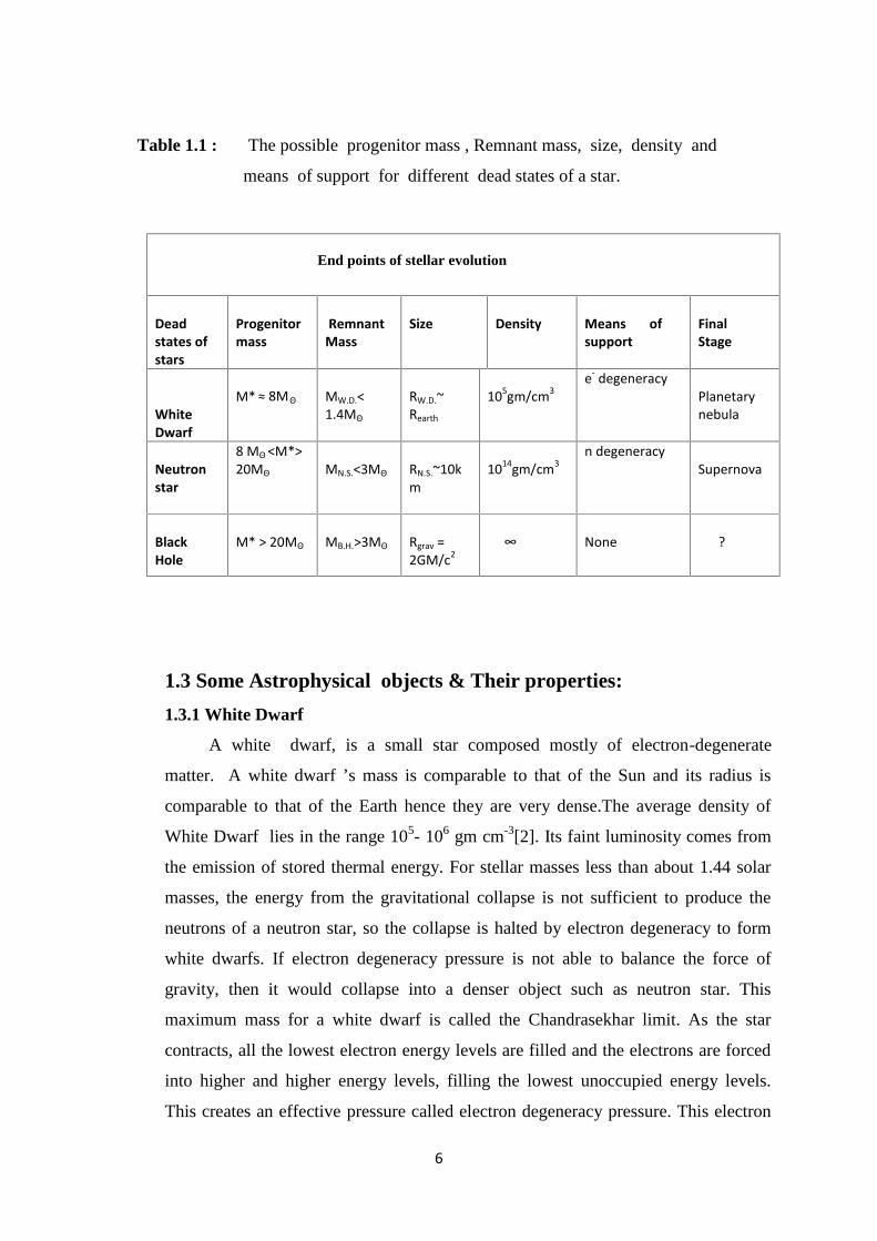
Table 1.1 : The possible progenitor mass , Remnant mass, size, density and
means of support for different dead states of a star.
1.3 Some Astrophysical objects & Their properties:
1.3.1 White Dwarf
A white dwarf, is a small star composed mostly of electron-degenerate
matter. A white dwarf ’s mass is comparable to that of the Sun and its radius is
comparable to that of the Earth hence they are very dense.The average density of
White Dwarf lies in the range 105- 106 gm cm-3[2]. Its faint luminosity comes from
the emission of stored thermal energy. For stellar masses less than about 1.44 solar
masses, the energy from the gravitational collapse is not sufficient to produce the
neutrons of a neutron star, so the collapse is halted by electron degeneracy to form
white dwarfs. If electron degeneracy pressure is not able to balance the force of
gravity, then it would collapse into a denser object such as neutron star. This
maximum mass for a white dwarf is called the Chandrasekhar limit. As the star
contracts, all the lowest electron energy levels are filled and the electrons are forced
into higher and higher energy levels, filling the lowest unoccupied energy levels.
This creates an effective pressure called electron degeneracy pressure. This electron
End points of stellar evolution
Deadstates ofstars
Progenitormass
RemnantMass
Size Density Means ofsupport
FinalStage
WhiteDwarf
M* ≈ 8MΘ MW.D.<1.4MΘ
RW.D.~Rearth
105gm/cm3e- degeneracy
Planetarynebula
Neutronstar
8 MΘ <M*>20MΘ MN.S.<3MΘ RN.S.~10k
m1014gm/cm3
n degeneracySupernova
BlackHole
M* > 20MΘ MB.H.>3MΘ Rgrav =2GM/c2
∞ None ?
7
degeneracy pressure is what supports a white dwarf against gravitational collapse.
When a medium sized star nears the end of its life and has used up all of its
available hydrogen, it will slowly expand into a red giant which fuses helium into
carbon and oxygen. Once this process has completed, the star will throw off its outer
layers to form a planetary nebula. The core that remains will be a white dwarf
composed of carbon and oxygen nuclei compressed by gravity and stripped of their
electrons. This extremely dense matter makes up a stellar remnant (white dwarf).
Due to its very high density the classical equation of state for a perfect gas do not
apply for white Dwarf , instead the pressure is given by the equation of state for
degenerate matter that is dense , cold matter [3].
1.3.2 Neutron star:
A neutron star is about 20 km in diameter and has mass of about 1.4 times that
of our sun. Because of its small size and high density, a neutron star possesses a
surface gravitational field about 2 × 10¹¹ times that of the earth. A NS is made up of
cold catalysed matter i.e. matter which has reached the end point of stellar evolution.
The magnetic field of the neutron star is of the order of ~ 1012 Gauss.
The temperature inside a newly formed neutron star is from around 1011 to 1012
Kelvin. However, the huge number of neutrinos it emits carry away so much
energy that the temperature falls within a few years to around 1 million Kelvin.
Neutron stars are known to have rotation periods between about 1.4 ms to 30
seconds. A neutron star's structure is very simple, and it has three main layers: A
solid core, a liquid mantle, and a thin, solid crust. Neutron stars also have a very tiny
(a few centimeters - about an inch) atmosphere, but this is not very important in the
functioning of the star. An approximation of neutron star dimension [4,5] is that it
has thick metallic surface layer, below which there is about 1 km thick solid layer of
material of density 105-1014 gm cm-3. Under this solid crust comes the main part of
the star which consists of a nuclear superfluid with a density of about nuclear
density. This superfluid core of NS comprises most of the mass of the star and
extends upto several km and holds itself up by neutron degeneracy pressure against
gravitational collapse. In the very centre of the star there is the possibility of the
existence of some

8
exotic matter. There may be pion condensate and probably a neutron solid and
hyperons.
1.3.3 Quasar (Quasi Stellar Object) :
Quasars are the most luminous, powerful, and energetic objects known in the
universe. They are the most distant known objects in the universe. The quasars ,
with total luminosity hundred times greater than that of giant galaxies, are
extremely unusual in their properties. The most luminous quasars radiate at a rate
that can exceed the output of average galaxies. Quasars have large red shifts
relative to normal stars and galaxies [6,7]. The accretion of material into super
massive black holes in the nuclei of distant galaxies is believed to be one of the
main cause of energy content of Quasar. All observed quasar spectra have redshifts
between 0.065 and 5.46 [8] .
If the lines in the spectrum of the light from a star or galaxy appear at a lower
frequency , the object exhibits positive red shift. The accepted explanation for this
effect is that the object must be moving away from us. Cosmological red shift is
seen due to the expansion of the universe. Gravitational red shift is a relativistic
effect observed in electromagnetic radiation of very compact objects. Quasars are
very high red shift objects indicating that they are very far away from us. The
brightest quasar is 3C273, two billion light years away from us . The red shift of
3C 273 is z = 0.158[9], meaning that the wavelengths of its spectral lines are
stretched by 15.8%. Models of Quasars have been proposed by Durgapal and
Gehlot and it has been shown that the maximum surface red-shift can be as large as
4.828[10] . We have also tried to construct the approximate models of Quasars in
chapter IV. The red shift has been also obtained for these models.
1.4 HOW A NEUTRON STAR IS FORMED :
Neutron stars are the product of supernovae, gravitational collapse events in
which the core of a massive star reaches nuclear densities and stabilizes against
further collapse. Neutron stars are one of the possible dead states for a star. They
result from massive stars which have mass greater than 4 to 8 times that of our Sun.
After these stars have finished burning their nuclear fuel, they undergo a supernova
9
explosion. This explosion blows off the outer layers of a star into a supernova
remnant. The central region of the star collapses under gravity. It collapses so much
that protons and electrons combine to form neutrons through the reaction .
enep (1.3)
The neutrinos escape the star. Enough electrons and protons must remain so that the
Pauli principle prevents neutron beta decay,
eepn (1.4)
The condition for the neutrons to be stable against beta decay is that the electron
Fermi sea should be filled up to a momentum greater than the maximum momentum
kmax of the electron emitted in neutron beta decay[11].
max, kk eF (1.5)
The neutron degeneracy pressure within the star counter balances the
gravitational collapse paving the way for the formation of neutron star. Neutron star
contains matter in one of the densest forms found in the universe. The pressure in the
star’s core is so high that most of the charged particles, electrons and protons, merge
resulting in a star composed mostly of uncharged particles called neutrons. The
central density of neutron star ranges from a few times the density of normal
nuclear matter to about one order of magnitude higher, depending on the star’s mass
and the equation of state. Neutron stars therefore provide us with a powerful tool for
exploring the properties of such dense matter. The discovery of pulsars by Hewish et
al. [12] have confirmed that they can be neutron stars only. Oppenheimer and
Volkoff [13] were the first to obtain the mass of neutron star within the framework
of general relativity. Oppenheimer and Volkoff concluded that the maximum mass
for neutron stars is 0.7 MΘ. Oppenheimer and Volkoff realized that for a neutron star
the modification of Newtonian gravity due to general relativity would have to be
taken into account. Although Oppenheimer and Volkoff had properly taken into
account the gravitational effects, they had assumed that the neutrons could be
regarded as an ideal fermi gas. The assumption of an ideal gas is quite valid for
electrons, but is a very poor assumption for neutrons. A gas may be regarded as an
ideal if the energy of interaction between the particles can be neglected. For more
realistic modeling of neutron star nucleon-nucleon interaction must be taken into
account.

10
1.5 The maximum mass limit for Neutron star:
The maximum mass of neutron star is a quantity of great importance to study
the final stages of stellar evolution. The upper mass limit is needed to distinguish a
neutron star from a black hole. The Tolman–Oppenheimer –Volkoff limit is an
upper bound to the mass of stars composed of neutron-degenerate matter i.e. neutron
star. The TOV limit is analogous to the Chandrasekhar limit for white dwarf
stars. This limit was obtained by J. Robert Oppenheimer and George Volkoff
in 1939, using the work of Tolman. Oppenheimer and Volkoff assumed that the
neutrons in a neutron star formed a degenerate cold Fermi gas. They obtained a
mass of approximately 0.7 solar masses at a radius of 9.6 km[11]. A black hole
formed by the collapse of an individual star must have mass exceeding the Tolman–
Oppenheimer–Volkoff limit.
The maximum mass limit for neutron star has been discussed by many authors
drawing different conclusions. Arnett and Bowers [14] have estimated the upper
mass limit as 1-3 MΘ. Rhodes and Ruffini [15] have estimated the upper mass limit
as 3.2 MΘ. Brecher and Caporasso [16] suggest this limit as 4.8 MΘ. Kamfer finds a
limit 3.75 MΘ [17]. Buitrago and mediavilla [18] found an upper limit of about 2 MΘ
for gravitational collapse in stars of uniform density in the neutron phase. The
maximum mass predicted by the various stiff equations of state is larger than the
measured masses of radio pulsars. Durgapal and Rawat [19] estimated the mass of
neutron star as 3.34 MΘ, when everywhere the speed of sound remains less than the
speed of light. Durgapal et al. [20] have obtained exact solution for a massive fluid
sphere under the extreme causality condition 1
d
dp. They obtained the maximum
mass of neutron star as 4.8 MΘ and size as 20.1 km. Pant et. al [21] have estimated
the maximum mass of neutron star as 6.33 MΘ with linear dimension 48.08 km . We
have also estimated the maximum mass of neutron star by obtaining exact solutions
of Einstein’s field equations in Chapter II.

11
1.6 Neutron star as pulsar:
Pulsars are spinning neutron stars that emit sharp pulses at exactly spaced
intervals of time [12]. Pulsar is a highly magnetized, rapidly rotating neutron
star[22]. Neutron stars are very dense, and have short, regular rotational periods. This
produces a very precise interval, between pulses that range from roughly
milliseconds to seconds for an individual pulsar. Extremely short periods of pulsars ,
suggests that pulsars are rotating neutron stars possessing a superhigh magnetic field
[23] and [24,25]. Neutron stars have very intense magnetic fields, as compared to
Earth's magnetic field. However, the axis of the magnetic field is not aligned with the
neutron star's rotation axis. The magnetic axis of the pulsar determines the direction
of the electromagnetic beam . Millisecond pulsars have provided us with best
working ground for testing of general relativity. The suggestion that pulsars were
rotating neutron stars was put forth independently by Thomas Gold and Franco Paciii
in 1968, and was soon proven by the discovery of a pulsar with a very short ( 33-
millisecond ) pulse period in the Crab nebula. The discovery of a pulsar at the centre
of crab-nebula, where the astronomers had predicted NS, established the oneness of
NS and pulsars.
The close observation of the pulsars can help to elucidate the interior
properties of neutron stars and can provide us with windows into the interiors of
neutron stars. The discovery of pulsars allowed astronomers to be acquainted with
the conditions of an intense gravitational field. We have also constructed the
approximate models of pulsars (Crab pulsar and vela pulsar) in chapter II.
1.7 The equation of state for Neutron star:
The equation of state for a neutron star is still not known exactly. Being both
very compact and extremely dense, neutron stars are unique laboratories for
probing the equation of state of neutron- rich matter . To have a complete picture of
NS a deep physical insight into the equation of state for dense 14105E gm cm-3
strong interacting hadronic matter is necessary. Despite a large amount of work
that has been done in literature on neutron star and equation of state of matter at
nuclear densities, the final picture regarding the properties of matter at super nuclear
densities is yet to be clearly understood .The structure of neutron stars is sensitive to

12
the equation of state of cold, fully catalysed, neutron-rich matter over an enormous
range of densities [26-28]. It is assumed that EOS for a neutron star differs
significantly from that of a white dwarf, whose EOS is that of a degenerate gas
which can be described in close agreement with special relativity. However, with a
neutron star the increased effects of general relativity can no longer be ignored.
Several EOS have been proposed for neutron star and current research is still
attempting to make predictions of neutron star matter. An understanding of an
equation of state is needed to estimate the parameters i.e. mass, size etc. of neutron
stars.
The mass of neutron star is an important parameter because after knowing the
mass of a neutron star only we can have an idea of the mass of black hole. A neutron
star requires many equations of state to completely describe the internal structure of
star.
The important density regions inside neutron star are as follows :
(i) 15 g cm-3 ≤ ρ ≤ 104 g cm-3; The Fermi- Thomas statistical model gives the
equation of state in this region [29].
(ii) 104 g cm-3 ≤ ρ ≤ 107 cm-3; In this region matter is so compressed that all
atoms are fully ionized, and we have a regular Coulomb lattice of nuclei,
neutralized by a gas of degenerate electrons; this is the outer crust [30]. The
electrons become relativistic at the upper end of the density range of this region.
(iii) 107 g cm-3 ≤ ρ ≤ 1011 g cm-3; Protons are converted into neutrons through
inverse beta decay process. The nuclei become more and more neutron rich.
(iv) 1011 g cm-3 ≤ ρ ≤ 4.5×10¹² g cm-3 ; at ρ = 1011 g cm-3, the nuclei become very
neutron rich and neutron begins to drip out of the nuclei. Neutron degeneracy
pressure increases with increase in density. The material consists of nuclei,
degenerate electrons and neutrons.
(v) 4.5×10¹² g cm-3 ≤ ρ ≤ 1014 g cm-3; in this region there is a giant nucleus
composed of three degenerate gases, viz. electrons, protons and neutrons. The
number density of protons and electrons is much lesser as compared to that of
neutrons.
(vi) 1014 g cm-3 ≤ ρ ≤ 1016 g cm-3; in this region along with neutrons , electrons
and protons, other elementary particles such as muons, pions and baryons may
also appear. At still higher densities the composition remains somewhat

13
uncertain, although hyperons, meson condensates or even deconfined quarks
might appear [31, 32].
1.8 The Coordinate Systems used in the present investigations:
The infinitesimal distance between two adjacent points in four dimensional
Riemannian space-time is given by
jiij dxdxgds 2
( 1.6)
Where ijg is the metric tensor in coordinates ( x1, x2 , x3 , x4 ) .
Here ( x1, x2 , x3 ) are space- like coordinates and x4 is time- like coordinate.
If we assume the spherical polar coordinates (r, θ, φ, ct ) , the coordinate r
increases as we move outwards from centre of the system. A gravitational system
is said to be spherically symmetric with origin at O, if the system is invariant
under spatial rotations about O. By rotational symmetry the metric properties on a
given sphere will be independent of the choice of θ and φ. The metric having this
property is given by
d Ω2 = (dθ2 + sin2θ dφ2 ) (1.7)
Thus, the spherically symmetric static space- time metric in Canonical or
curvature co-ordinates is given by
22222222 sin drdrdredteds (1.8)
Here λ and ν are functions of r.
The static, spherically symmetric space- time metric in isotropic coordinate
system is given by
22222222 sin dtceddrdreds (1.9)
Here coordinates (r, θ, φ, ct ) , are referred to as isotropic Coordinates and α,
β are functions of r. For non static case α and β will be functions of both r and t.
The another form of metric that is useful in the present study is spherically
symmetric non static metric conformal to the flat space time metric and will be
given by

14
222222222 sin),( ddrdrdtctrAds (1.10)
Where A is function of both r and t.
1.9 Einstein’s Field Equations and their importance :The line element of a static spherically symmetrical system is given by
22222222 sin drdrdredteds (1.11)
Where ν and λ are functions of r alone.
For the spherically symmetric mass distribution described in curvature coordinates
by the metric (1.11 ) the field equation is given as [33, 34]:
Tc
GRgR
4
8
2
1 (1.12)
Where R is Ricci tensor, R is the curvature invariant and T is the energy
momentum tensor.
The energy momentum tensor T is defined as
PguucPT )( 2 (1.13)
where P denotes the pressure distribution , the density distribution andu the velocity vector.
For a static case
)0,0,0,( 2
eu (1.14)
The components of the energy momentum tensor of a perfect fluid are given by
200
33
22
11 , cTPTTT (1.15)
)(0 T (1.16)
By evaluating the values of R , Rand using eq. (1.13) the resulting field
equations for the metric given by eq (1.11) are as follows:
2224
00 1188
rrre
c
G
c
TG (1.17)
2244
11 1188
rrre
c
PG
c
TG (1.18)

15
4242
888 2
44
33
4
22
re
c
PG
c
TG
c
TG
(1.19)
Here we have a system of three differential equations with four unknowns P, ,
λ, ν. When we want to study static massive spheres in general relativity we seek
to obtain the four variables pressure (P), density ( ), red shift parameter (ν) and
volume correction factor (λ) as a function of radial distance (r) measured from the
centre of the sphere. Now as there are only three independent field equations
hence we need one more equation to get all the parameters. The fourth equation
may be taken in the following form.
(i) as a function of r (e.g. Wyman , Kuchowich , Tolman,s III, VI, and VII
solutions)[35-37].
(ii) ν as a function of r ( Durgapal and Pandey, Durgapal, Pant )[38-40].
(iii) λ as a function of r ( Kuchowich, Durgapal and fuloria )[41-42].
(iv) P as a function of (Shapiro et al., pandey et al.,)[43-44].
From equations (1.18) and (1.19) ,Tolman [37] obtained following differential
equation
r
e
dr
de
r
e
dr
d
r
e
dr
d
22
12
(1.20)
By assuming various possible relations among ν and λ , Tolman has solved the above
equation and has found eight solutions of Einstein’s field equations.
For the space-time outside the mass distributions the solution is as follows:
arforarforP 0,0 (1.21)
arforr
mee
21 (1.22)
Eqs.(1.21) and (1.22) express exterior Schwarzschild solution which depends only
upon the configuration mass and not at all upon the details of mass distribution as long
as the distribution is spherically symmetric [45].
16
In geometrical units popular in General relativity, the unit of length is metre: but that
of mass and time are so chosen that the Gravitational Constant G and the speed of light
c are equal to unity i.e. c = G =1.
In geometrical units equations (1.17) , (1.18) and (1.19) will reduce to the following
form
224
4
1188
rrreT
(1.23)
221
1
1188
rrrePT
(1.24)
4242888
23
32
2
rePTT (1.25)
The equations (1.23) to (1.25) along with a fourth equation of the following form
P = P(ρ) , )(r , )(r , )(r (1.26)
can be computed to obtain various physical parameters of the stellar structure viz.
p, ρ, ν and λ under consideration.
The study of the relativistic stellar structures involves solutions of Einstein’s field
equations. In order to visualise a clear picture of the interior, one should obtain
exact solution of the Einstein’s field equations and use the results to construct
stellar models.
1.10 Field Equations in isotropic coordinates:
The space-time metric in isotropic coordinates is given by
22222222 sin ddrdredtceds (1.27)
For the metric (1.27) the field equation (1.12) reduces to the following equations
rrep
c
G
24
8 2
4
(1.28)

17
rr
pc
G
22422
8 2
4
(1.29)
re
c
G
2
4
8 2
2
(1.30)
where prime ( ' ) denotes the differentiation with respect to r .
From (1.28) and (1.29) we obtain following differential equation in α and β
0
22
22
rr
(1.31)
The new solution of Eq. (1.31) can be explored by considering various possible
relations among the unknown variables. However, the solution must satisfy all
the necessary conditions to be physically realizable.
1.11 Local maxima and local minima at the centre:
In order to study the trend of physical variables , following theorem may be
useful:
Theorem-
If xlrk ;0
xdx
dland
02
2
xdx
ldare nonzero finite, where 2rx ,
Then (i) maxima of k(r) will exist at r = 0 if0
xdx
dlis finitely negative.
(ii) minima of k( r) will exist at r = 0 if0
xdx
dlis finitely nonzero positive.
Proof : For maxima and minima we have
0,002)(0
xdx
dlasr
dx
dlr
dr
dx
dx
dlrk
dr
d
(1.32)

18
00
2
22
002
2
2422
rrrrdx
dl
dx
ldr
dx
dl
dx
dlr
dr
drk
dr
d, (1.33)
Provided0
2
2
xdx
ldis finite.
For the maximum at the centre (r = 0)
0200
2
2
xrdx
dlrk
dr
d
(1.34)
For the minima at the centre (r = 0)
0200
2
2
xrdx
dlrk
dr
d
(1.35)
This theorem is useful for showing the monotonically decreasing or increasing
nature of various physical parameters for well behaved nature of the solution.
1.12 Darmois Conditions (Junction conditions in isotropiccoordinates):
A solution of the field equation (1.20) for spherical matter distribution will be
valid in the space - time region occupied by the matter. If no matter exists
outside this spherical distribution then the laws governing the space time geometry
in the exterior region will be given by
0R (1.36)
The space- time must be continuous at the junction of interior space time region
and the exterior space time region. The geometry of the junction hyper surface
should satisfy eqs.(1.12) and (1.36) simultaneously. Three different sets of
boundary conditions have been given by Darmois , Lichernowicz , Brian and
Syange. The conditions due to Darmois and Lichernowicz are equivalent.
The Darmois set of condition is most convenient and reliable [46].
The exterior space–time metric to the static fluid ball in isotropic coordinate is
given by.
19
222222
1
222
22 sin
21
21 dRdRdR
Rc
GMdtc
Rc
GMds
(1.37)
Where t and R are the time and the radial coordinates respectively of the
exterior region. M is a Schwarzschild mass of the ball. The time coordinate t is
same for both the interior and exterior region, since the fluid ball is static so
time will be same for exterior also.
According to Darmois conditions the metric coefficients ijg and their first
derivatives kjig , in interior solution as well as in exterior solution should be
continuous upto and on the boundary B. The continuity of metric coefficients ijg of
interior and exterior space-time metric on the boundary is known first
fundamental form. The continuity of derivatives of metric coefficients gij of
internal and external solutions on the boundary is known second fundamental
form.
Since Schwarz schild’s metric (1.37) is considered as the exterior solution, the
following conditions are obtained by matching first and second fundamental
forms with canonical coordinate metric (1.8).
Rb = rb (1.38)
bRc
GMe b
2
21
(1.39)
bRc
GMe b
2
21
(1.40)
2
1
222 2
12
1
bb Rc
GM
Rc
GMe
b
(1.41)
Equations (1.38) to (1.41) are four conditions, known as boundary conditions in
canonical coordinates. Equations (1.38) and (1.41) are equivalent to zero pressure of
interior solution on the boundary. Similarly by matching the Schwarzschild’s metric
(1.37) with the isotropic coordinate metric (1.27) we arrive at the following
conclusions:
bRc
GMe b
2
21
(1.42)
20
2b
erR bb
(1.43)
2
1
2
21
2
2
1
bb
b Rc
GMr
r
(1.44)
2
1
22
21
2
1
bbb Rc
GM
Rc
GMr (1.45)
Equations (1.42) to (1.45) are four conditions, known as boundary conditions in
isotropic coordinates. Equations (1.43) and (1.45) are equivalent to zero
pressure of interior solution on the boundary.
1.13 Exact Solutions of Einstein’s Field equation:
Stellar Relativistic models have been studied ever since the first solution of
Einsein's field equation was obtained by Schwarzschild for the interior of a
compact object in hydrostatic equilibrium. The search for the exact solutions is
of continuous interest to physicists because a well behaved solution of Einstein’s
field equation can give us a deep insight into the interiors of massive fluid spheres.
The Einstein field equations describe the fundamental interaction of gravitation
as a result of space time being curved by matter and energy. The Einstein field
equations are complicated in nature. They are coupled, nonlinear partial differential
equations, Hence, it is very hard to solve them. The nonlinearity of the Einstein’s
field Equations distinguishes general relativity from many other fundamental
physical theories where we come across the linear equations. Despite the non linear
character of Einstein’s field equations, various exact solutions for static and
spherically symmetric metric are available in the literature.
The first two exact solutions of Einstein’s field equations were obtained by
Schwarzschild [47]. The first solution corresponds to the geometry of the space-time
exterior to a prefect fluid sphere in hydrostatic equilibrium. While the other solution
describes the interior geometry of a fluid sphere of constant energy-density E and
known as interior Schwarzschild solution. Tolman [37] obtained five different types

21
of exact solutions for static cases. The III solution corresponds to the constant
density solution obtained earlier by Schwarzschild [47]. The V and VI solutions
correspond to infinite density and infinite pressure at the centre, hence not considered
physically viable. Thus only the IV and VII solutions of Tolman are of physical
relevance. The VII solution has been studied extensively by Durgapal and Rawat[19].
The various other solutions of Einstein’s field equations have been obtained
by Adler [48], Adams and Cohen [49], and Kuchowicz [50], Buchdahl’s solution
[51] for vanishing surface density. The solution obtained by Vaidya and Tikekar
[52], has also been obtained by Durgapal and Bannerji [36]. The class of exact
solutions has been obtained by Durgapal [38]. Durgapal and Fuloria [42] solution is
also physically realizable. The most general exact solution for isentropic superdense
star was obtained by Gupta and Jasim [53]. Durgapal et al. [54] have tested the
suitability of the exact solutions for application to the stellar models . Pant, N.[ 55]
has presented three new categories of exact and spherically symmetric solutions of
Einstein’s field equations and obtained the mass of neutron star as 3.369 MΘ with
linear dimension 37.77 km. The various solutions of Einstein’s Field Equations that
are available in literature can be categorized as follows:
Category I
If the solutions are well behaved and regular (Delgaty and Lake [56]; Pant et al.
[57] ), these solutions completely describe interior of the neutron Star and other
compact stellar objects. The latest account of these solutions has been furnished by
Delgaty and Lake [56] and they found that only nine of them are regular and well
behaved. Out of which only six are well behaved in curvature coordinates and rest
three solutions are in isotropic coordinates.
Category 2-
If the solutions are not regular and well behaved but with finite central
parameters, such type of solutions may be used as seed solutions of super dense star
with charge matter since at the centre the charge distribution is zero. Many of the
authors electrified the well known exact solutions which are not well behaved e.g.
Kuchowich solution [58] by Nduka [59], Adler solution [60] by singh and
Yadav[61] ; by Pant and Tewari [62], Tolman solution [37] by Cataldo and

22
mitskievic [63], Heintzmann solution [64] by Pant. N, et al. [65]. These solutions are
useful for describing the interior of superdense astrophysical objects with charge
matter.
1.14 Charged fluid spheres in General Relativity:
The neutral solutions of Einstein’s field equations have very important
astrophysical implications. The Various compact stellar objects like neutron star,
white Dwarf, pulsar can be explained theoretically by studying the physically
realizable solutions of Einstein’s field equations. But many solutions of Einstein’s
field equations are not well behaved , hence can not be used for modeling of
astrophysical objects. The solutions of Einstein’s field equations which are not well
behaved in neutral arena can be made well behaved after including charge in them .
The charged interior solutions of Einstein field equations are normally found very
useful to predict or explain the various properties of massive compact objects. It is
observed that in the presence of charge, the gravitational catastrophic collapse of a
spherically symmetric material ball to a point singularity can be avoided by virtue of
the Columbian repulsive force along with the thermal pressure gradient. Exact
solutions of Einstein-Maxwell field equations are important in the modeling of
relativistic astrophysical objects. Such models successfully explain the characteristics
of massive objects like Neutron stars, Pulsars, Quark stars, or other super-dense
objects.

23
1.15 Einstein’s –Maxwell equations for charged fluid distribution:
Let us consider a spherical symmetric metric in curvature coordinates
22222222 )sin( dtedrdrdreds (1.46)
where the functions )(r and )(r satisfy the Einstein-Maxwell equations
mn
mnijjm
imij
jiij
ij
ij FFFFpvvpc
c
GRRT
c
G
4
1
4
1)(
8
2
18 244
(1.47)
where , p, iv , Fij denote energy density, fluid pressure, velocity vector and skew-
symmetric electromagnetic field tensor respectively.
In view of the metric (1.46), the field equation (1.47) gives
4
2
42
81
r
qp
c
G
r
ee
r
(1.48)
4
2
4
2 8
2442 r
qp
c
Ge
r
(1.49)
4
2
22
81
r
q
c
G
r
ee
r
(1.50)
where prime ( ' ) denotes the differentiation with respect to r and q(r) represents the
total charge contained with in the sphere of radius r.
24
1.16 Mathematical formulation of red shift:Gravitational red shift is the process by which electromagnetic radiation
originating from a high gravity star is reduced in frequency or red shifted, when
observed in a region of a weaker gravitational field. The red shift of the spectral
lines of the light originating from the dense stars is an important effect of the
gravitational field. This is the manifestation of slowing down of the time in the
gravitational field. The trajectory of light is null and is represented by ds = 0.The
speed of light originating at any position is given in terms of coordinate distance r
and coordinate time t by [66]
r
me
dt
dr 212
for Schwarzchild geometry (1.51)
a
m21 (at the surface of the star) (1.52)
For a fixed direction θ and may be taken as constants. From Eq.(1.51) we see
thatdt
dris independent of time t. Hence it may be concluded that the successive
pulses of light separated by the time t would always be separated by the
coordinate period of the observer. To the same interval of world time t , there
correspond at different points of space different intervals of proper time . The
relation between the proper period and coordinate period is given by [66]
2
1
21
r
mts
(1.53)
2
1
00gt (1.54)
2
et (1.55)
Let 0f = The frequency emitted from star = proper frequency
= number of oscillations per unit proper time
=
stellard
dN
(1.56)

25
ef = Observed frequency on earth
earthd
dN
Thus2
1
00
000
)(
)(
earthg
stellarg
f
f
e
(1.57)
If instead of earth the observer is at rest at a spatial infinity, the frequency
observed by the observer will be given by:
dt
d
d
dN
dt
dNf
(1.58)
= 2
1
000 gf (1.59)
Equations (1.57) and (1.59) show that instead of observing a frequency 0f , we
observe a reduced frequency. Hence the observed wavelength will be larger and
the red shift can be expressed as
2
1
000
1 gZ g
(1.60)
= 2
)(r
e
(1.61)
Where Zg is called the gravitational red shift.
1.17 Radiating Fluid Distribution & gravitational Collapse:
In a normal star the stellar radiation is a very slow process and any change
in the interior and exterior gravitational field is generally insignificant. However,
the situation is different for high energy astrophysical objects such as quasars and
supernova burst, where this radiation process is very strong. Therefore it is
desirable to study the solution of general relativistic field equations in terms of the
out flowing radiation. For the consideration of the above astrophysical problem
in the frame work of general relativity a proper mathematical formulation is
26
desirable. For a general relativistic treatment of strong gravity objects like Quasar
a radiating fluid ball is a close model.
It is already established fact that gravitational collapse is highly dissipating
energy process which plays a dominant role in the formation and evolution of
stars. However, the dissipation of energy from collapsing fluid distribution is
described in two limiting cases. The first case, the free streaming approximation
applies whenever the mean free path of particles responsible for the propagation of
energy in the stellar interior is larger (or equal to) than the typical length of the
object. In this case dissipation is modeled by means of an out flowing null fluid.
The second case, the diffusion approximation applies when the mean free path of
particles responsible for the propagation of energy in stellar interior is very much
small as compared with the typical length of the object . In this case dissipation is
modeled by means of a heat-flow type vector. The models of radiating fluid
spheres have been constructed both in free streaming case and in diffusion case by
many authors.
Following Tolman’s approach [37] , Vaidya [67-68] initiated the problem
for physically meaningful models of radiating fluid spheres in free streaming
limiting case. Bayin [69] has obtained exact solutions describing radiating perfect
fluid spheres. Some of them are physically reasonable but some are not
physically sound. Herrera et al. [70] have proposed a method to construct
radiating fluid ball models from the known static solutions of Einstein’s field
equations. Solutions for the radiating fluid ball problem corresponding to isotropic
coordinates form and in general metric form have been discussed by Tiwari [71-
72]. The radiating fluid sphere in conformally flat metric form has been discussed
by Pant and Tiwari [73]. Santos [74] has extensively studied the model proposed
by Glass [75] and has discussed the boundary conditions at the junction of the
interior and exterior metrics. The interior space time metric is matched with
vaidya’s exterior space-time metric.

27
1.18 Hydrodynamics of the Radiating Fluid spheres:
The most general space-time metric in spherical polar coordinates (ct, r, θ,
) which describes the geometry of a dynamic spherical distribution of matter
energy is expressed as
22222222 sin dderdredtceds (1.62)
Where ),(),,(,),( trtrtr ,
We have used the metric (1.62) because it is consistent with the system of
coordinates co moving with the matter particles of the distribution.
The Einstein’s field equations for space-time region occupied by matter energy
are expressed as:
ijjiji Tc
GgRR
4
8
2
1
(1.63)
i , j takes the values 0,1,2,3.
Rij is contracted curvature tensor, R is the scalar curvature, G is the Newtonian
constant of gravitation.
For a radiating fluid ball we can divide Tij into two parts. One part represents the
matter content of the distribution and the other part represents the radiation:
radiation
ijmatter
ij
ij TTT
(1.64)
To simplify the problem we assume that the fluid ball is composed of perfect fluid
through which energy is flowing out in the radial direction. For a perfect fluid we
have
ij
ijmatter
ij gpvvcpT 2 (1.65)
Here p and ε respectively denote the isotropic pressure and density of a perfect
fluid particle measured in its local rest frame and vi its unit time –like four-
velocity.
1iivv (1.66)
28
The energy momentum tensor for the radiation is given by
jiradiation
ij ww
c
qT (1.67)
where q is the rate of radiation or the rate of flow of energy.
w i its four velocity which is null:
0ii ww (1.68)
If the fluid distribution and its motion is spherically symmetric , we have
032 vv (1.69)
We assume that the radial coordinate r is co moving with fluid particles, so that
01 v (1.70)
From ( 1.62), (1.66) and ( 1.70) we have
20
ev (1.71)
The outward flow of radiation is in the radial direction only so that
032 ww (1.72)
From (1.68) and (1.72) we get
120 wew
(1.73)
if 1w is known we can determine iw completely .
The components of ijT in co moving coordinates are given by
11
11 ww
c
qpT
(1.74)
PTT 33
22 (1.75)
29
00
200 ww
c
qcT
(1.76)
01
01 ww
c
qT
(1.77)
1.19 Vaidya Metric and its derivation:
The geometry outside a spherically symmetric star when the exterior is
taken to be non–empty due to radiation from the star is given by the Vaidya metric
[67, 76]. The Vaidya metric describes exterior gravitational field due to a radiating
star. A spherically symmetric body that emits a continuous stream of photons with
each photon travelling radially outwards will be described by a metric that will
have energy- momentum tensor of the radially outgoing null rays. The Vaidya
metric is capable of describing this situation and provides an interesting model for
a time dependent spherically symmetric metric.
The space-time metric outside a radiating stellar object can not be defined by
Schwarzschild metric as it corresponds to an empty exterior given by Tij = 0. In
the case of a normal star, the effect of radiation on the overall exterior space-time
could be negligible. However the radiation effects would be important during the
late stages of gravitational collapse when the star could be throwing away
considerable mass as radiation or when abundant neutrinos are radiated away
from a collapsing supernova core. Such a radiating stellar object would then be
surrounded by an ever expanding zone of radiation. Vaidya metric is a simple and
interesting generalization of the Schwarzschild metric, which can be interpreted as
a space time with an outgoing spherically symmetric radiation of mass less
particles.
The energy- momentum tensor in the region permeated by radial energy flux with
null four- velocity wi and density q is given by
jiij wwc
qT (1.78)
With 032 ww and
30
011
00 wwww (1.79)
The field equations to be solved are
ijijij Tc
GgRR
4
8
2
1 (1.80)
In the canonical coordinates ( ct, R, θ, ) the space-time metric will be of the form
22222,22,2 sin ddRdRedtceds TRTR (1.81)
In radiation coordinates ( u, R, θ, ) eq. (1.81) transforms into
dRedTcefdu 221
(1.82)
Here TRf , is an integrating factor. The metric (1.81) then takes the form [77]
22222222 sin2
ddRdRduefdufds (1.83)
In this form Vaidya obtained a solution of (1.81) which is given below:
222222
2 sin2)(2
1 ddRdRduduRc
uMGds
(1.84)
At spatial infinity (R = ∞) the space-time is flat. Also when M is a constant, the
metric reduces to that due to Schwarzschild. We call M(u) Vaidya mass and u the
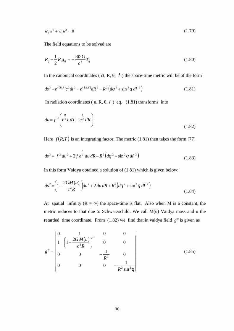
retarded time coordinate. From (1.82) we find that in vaidya field ijg is given as
22
2
1
2
sin
1000
01
00
002
11
0010
R
R
Rc
uMG
g ij (1.85)
31
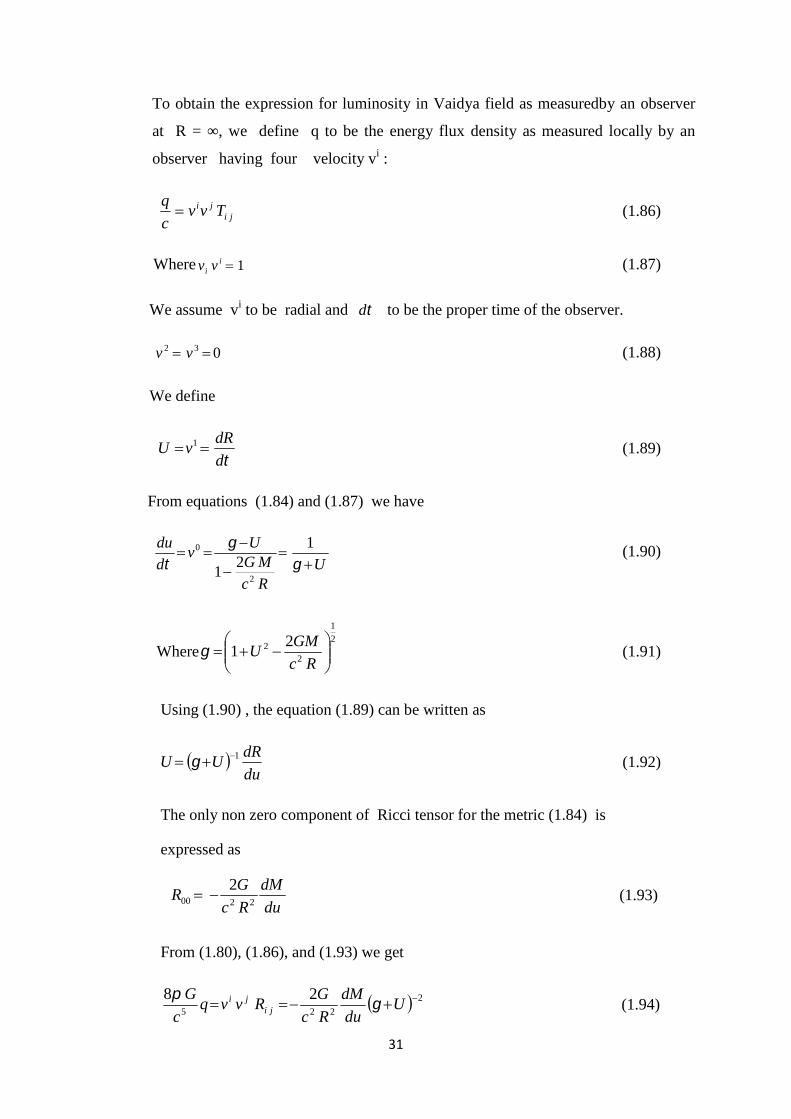
To obtain the expression for luminosity in Vaidya field as measuredby an observer
at R = ∞, we define q to be the energy flux density as measured locally by an
observer having four velocity vi :
jiji Tvv
c
q (1.86)
Where 1ii vv (1.87)
We assume vi to be radial and d to be the proper time of the observer.
032 vv (1.88)
We define
d
dRvU 1 (1.89)
From equations (1.84) and (1.87) we have
URc
MGU
vd
du
1
21
2
0 (1.90)
Where2
1
22 2
1
Rc
GMU (1.91)
Using (1.90) , the equation (1.89) can be written as
du
dRUU 1 (1.92)
The only non zero component of Ricci tensor for the metric (1.84) is
expressed as
du
dM
Rc
GR
2200
2 (1.93)
From (1.80), (1.86), and (1.93) we get
2
225
28 Udu
dM
Rc
GRvvq
c
Gji
ji
(1.94)
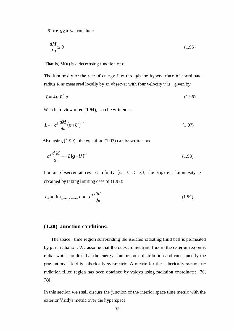
32
Since 0q we conclude
0ud
dM(1.95)
That is, M(u) is a decreasing function of u.
The luminosity or the rate of energy flux through the hypersurface of coordinate
radius R as measured locally by an observer with four velocity vi is given by
qRL 24 (1.96)
Which, in view of eq.(1.94), can be written as
23 Udu
dMcL (1.97)
Also using (1.90), the equation (1.97) can be written as
12 ULd
Mdc
(1.98)
For an observer at rest at infinity RU ,0 , the apparent luminosity is
obtained by taking limiting case of (1.97):
du
dMcLL UR
30,lim (1.99)
(1.20) Junction conditions:
The space –time region surrounding the isolated radiating fluid ball is permeated
by pure radiation. We assume that the outward neutrino flux in the exterior region is
radial which implies that the energy –momentum distribution and consequently the
gravitational field is spherically symmetric. A metric for the spherically symmetric
radiation filled region has been obtained by vaidya using radiation coordinates [76,
78].
In this section we shall discuss the junction of the interior space time metric with the
exterior Vaidya metric over the hyperspace

33
r = rs (1.100)
where rs is a constant, or equivalently R = Rs(u) (1.101)
Suffix s denotes the value of the quantities over the hyper surface (1.100). For
smooth junction of the two space-time regions, Darmois conditions (1927) are to
be satisfied by the geometries of the two regions over the common boundary.
These conditions state that across the boundary the first and the second
fundamental forms should be continuous.
These boundary conditions have been obtained for the radiating fluid sphere by
Misner [79].
The continuity of the first fundamental forms across the hyper surface (1.100)
implies that the interior metric and the exterior metric must match over the hyper
surface.
This leads to the following equations
)(
,2
1
uRer s
tr
s
s
(1.102)
dudu
dR
Rc
GMdtce s
s
trs
2
1
2, 2
21
(1.103)
dt
dReU str
ss 2/,
(1.104)
In view of eq.(1.104), eq.(1.103) can be rewritten as
2
1
2
22/, 21
sss
tr
Rc
GMUU
du
dtce s
(1.105)
From (1.92), (1.104), (1.105) the following relation is obtained.
ss UU (1.106)
The continuity of the second fundamental form across (1.100) leads to the following
equations
34
0, trp s (1.107)
uMtrm s , (1.108)
The expression for the luminosity as observed at infinity is given by
du
dMcL 3 (1.109)
All these relations are useful for the study of radiating fluid spheres.
(1.21) Gravitational Collapse:
Gravitational collapse is the inward fall of a body due to the influence of its
own gravity. In any stable body, this gravitational force is counterbalanced by the
internal pressure of the body, in the opposite direction to the force of gravity.
Gravitational collapse is usually associated with very massive bodies, such as
neutron stars, quasars and massive collections of stars such as globular clusters
and galaxies .
Gravitational collapse is at the heart of structure formation in the universe. For
example, a star is born through the gradual gravitational collapse of a cloud of
interstellar matter. The compression caused by the collapse raises the temperature
until nuclear fuel reignites in the centre of the star and the collapse comes to a
halt. The thermal pressure gradient compensates the gravity and a star is in
dynamical equilibrium between these two forces. After a star has exhausted its
nuclear fuel, it can no longer remain in equilibrium and must ultimately undergo
gravitational collapse.
The importance of gravitational collapse processes in relativistic astrophysics
was realized when Datt [80] and oppenheimer and Synder [81] used general
relativity to study the dynamical collapse of a homogeneous Spherical dust cloud
under its own gravity. This model gave rise to concept of a black hole. A black
hole is a region of space time from which no light or matter can escape away to
far away external observers. In order to create a black hole as the final state of
35
gravitational collapse of the star, an event horizon must develop in the space time
earlier than the time when the final space time singularity forms.
If the event horizon is developed prior to the formation of the singularity , neither
the singularity nor the collapsing matter that has fallen within it would be observable
to an external observer, and a black hole is said to have formed as the final end state
of the collapsing star. The event horizon is where light loses the ability to escape
from the black hole.
1.22 Naked Singularity &Cosmic Censor Hypothesis:
In General Relativity , a naked singularity is a gravitational singularity , without
an event horizon . In a black hole, there is a region around the singularity, the event
horizon, where the gravitational force of the singularity is strong enough so that light
cannot escape. Hence, the singularity cannot be directly observed. A naked
singularity, by contrast, is observable from the outside. Radiating stellar models have
been proposed by Bannerjee et al. [82] in which the horizon is never encountered and
naked singularity comes into existence. Pant, N. and Tewari, B. C. [83] have also
discussed the horizon –free gravitational collapse of radiating fluid spheres .
The theoretical existence of naked singularities is important because their
existence would mean that it would be possible to observe the collapse of an
object to infinite density. A naked singularity could allow scientists to observe an
infinitely dense material, which would under normal circumstances be impossible
by the cosmic censorship hypothesis. The cosmic censorship hypothesis says that a
naked singularity cannot arise in our universe from realistic initial conditions.
According to cosmic censorship hypothesis conceived by Roger Penrose in 1969
no naked singularities other than the Big Bang singularity exist in the universe.
Cosmic Censorship Hypothesis states that the universe contains no singularities
that can be visible to a very far away observer.
We have investigated the models of radiating stellar objects (Quasars)
undergoing gravitational collapse in which the horizon is not formed i.e. the
collapse process will go on forever ultimately reaching to a point singularity called
36
a naked singularity. While constructing the models of radiating stellar objects in
chapter IV we have shown that the mass radius gradient is less than one, or
collapse is horizon free . Theoretically we can say that there is possibility of the
existence of naked singularity, the singularity that will be observable by external
observer.
1.23 Objective of the Thesis:
The exact solutions of Einstein’s field equations and Einstein - Maxwell field
equations provide us with a powerful tool for exploring the interior properties of
relativistic astrophysical objects. Due to nonlinearity of Einstein’s field equations
there is relative scarcity of exact solutions , however their significance in
understanding the interiors of stellar objects can not be ignored. Keeping in view the
relevancy of solutions of Einstein’s field equations and their application to various
astrophysical objects the present thesis embodies the exploration of some new
solutions of Einstein’s field equations , Einstein-Maxwell field equations and their
use in modeling of immense gravity objects. The most important tool for such
modeling is static, spherically symmetric exact solution with perfect fluid matter and
finite central parameters. The characteristics of massive objects like , neutron star,
pulsar or other super-dense objects can be successfully explained by these models.
The non static solutions of Einstein’s Field equations also have manifold importance
in understanding certain aspects of the astrophysical objects emitting a large amount
of energy in the form of radiation. The stellar objects emitting radiation also undergo
gravitational collapse and may end into either black hole or naked singularity.The
time dependent solutions of Einstein’s field equations are useful for understanding
such problems.
Consequently chapter II [84,85] deals with an attempt to find some new
solutions of Einstein’s field equations. One solution in curvature coordinates and
another one in isotropic coordinates have been found. The characteristics of these
solutions have been studied extensively. Keeping in view the well behaved nature
we have ventured into the modeling of compact stellar objects like neutron star.

37
Chapter III [86, 87] covers the study of well behaved , static charged fluidspheres. The presence of charge in massive fluid spheres has considerable impacton the overall properties of stellar objects. The gravitational collapse of the stellarobject to a point singularity can be avoided due to the repulsive effect of chargepresent in the fluid sphere. We have obtained a new generalized solution ofEinstein -Maxwell field equations which can provide us a series of well behavedsolutions. These solutions have been used for the modeling of immese gravityastrophysical objects. For this class of solutions the outmarch of pressure, density,pressure-density ratio and the adiabatic sound speed is monotonically decreasing.
Chapter IV is devoted to the extensive study of BCT solution II [71] for themodeling of radiating stellar objects. We have made an attempt to construct theapproximate models of Quasars for different combinations of the constants X, Yand Z appearing in the solution . The variation of pressure, density, pressure-density ratio and luminosity has been studied with in the radiating fluid sphere(Quasar) . It has been observed that the final outcome of the gravitational collapseof radiating fluid sphere will be naked singularity .
In Chapter V [ 88] we have studied adiabatic collapse of a uniform densitysphere [with Schwarzschild geometry in the exterior] using baryon conservationlaw and no-heat-transfer condition . It is concluded that a uniform density sphere[with Schwarzschild geometry in the exterior] always collapses adiabatically withvanishing pressure.In Chapter VI we have made an attempt to find a new time dependent solution ofEinstein’s field equations . Although the solution is singular at the centre but itmay give some insight in understanding the various phenomena concerned withradiating fluid spheres. We have also made an extensive study of non staticsolution obtained by Tewari [73] in conformally flat space time metric. It has beenshown that the solution is well behaved and may be useful for modeling ofradiating stellar objects.

38
1.24 References:
[1] Chandrasekhar, S. : “The highly collapsed configurations of a stellar
mass”, Mon. Not. R. Astr. Soc 95, 207 (1935).
[2] Baidyanath Basu , “ An Introduction to Astrophysics”, : Prentice hall of
India, Private Limited , pp. 319 (1997).
[3] Lloyd, Motz: “Astrophysics and Stellar Structure”, Printed in United
states of America. pp. 564 (1970).
[4] Baym, G., Pethick, C.J., Pines, D. and Ruderman, M. : “Spin Up in
Neutron Stars : The Future of the Vela Pulsar”, Nature, 224, 872
(1969).
[5] Ruderman, M. : “Pulsars: Structure and Dynamics”, Ann. Rev. Astron.
Astrophys. 10, 427 (1972).
[6] Schmidt, M. :“3c 273: A star- like object with Large red shift”, Nature
197, 1040(1963).
[7] Greenstein, J. L., Matthews Thomas, A. : “Red shift of the Radio Source
3C48”, Astronomical Journal, 68, 279(1963).
[8] Schneider, Donald P., Richards, Gordon T. et al.: “The Sloan Digital
Sky Survey Quasar Catalog. V. Seventh Data Release ”, The
Astronomical Journal, 139(6), 2360 (2010).
[9] Narlikar, J.V. : “An introduction to cosmology”,Cambridge University
Press, pp.21(2004).
[10] Durgapal, M.C., Gehlot, G. L.: “Massive spheres in relativity and large
gravitational red shift of Quasars”, Indian Journal of radio and Space
Physics 2, 287 (1973).

39
[11] Weinberg S. : “Gravitation and Cosmology: Principles and
Applications of the General Theory of Relativity”, John Wiley &
Sons, Inc.(U.S.A.) (1972).
[12] Hewish, A. , bell, S. J. , Pilkington, J. P. H., Scott, P. F. and Collins, R.
A. : “Observation of a Rapidly Pulsating Radio Source”, Nature 217,
709 (1968).
[13] Oppenheimer, J. R. and Volkoff, G. M .: “On Massive Neutron
cores”, Phys. Rev. 176, 1496 (1939).
[14] Arnett, W. D. and Bowers, R. L. : “A Microscopic Interpretation of
Neutron Star Structure”, Astrophys. J (suppl.) 33, 415 (1977).
[15] Rhodes, C. E. and Ruffini, R. : “Maximum Mass of a Neutron Star”,
Phys. Rev. Lett. 32 324 (1974).
[16] Brecher, K. and Caporasso, G. : “Obese 'neutron' stars”, Nature 259,
377 (1976).
[17] Kampfer, B. : “An Upper Bound on Neutron Star Masses”, Astron.
Nuclr. 305(4), 193 (1984).
[18] Buitrago, J. and Mediavilla : “The limit of mass for gravitational
collapse and nuclear forces at short distance”, Astrophys. & space Sci.
109, 407(1985).
[19] Durgapal, M. C., Rawat P. S.: “Non –rigid spheres in general
relativity”, Mon. Not. R. Astr. Soc. 192, 659(1980).

40
[20] Durgapal, M. C., Pande, A. K., Rawat, P.S. : “Extreme relativistic
model for neutron stars and pulsars”, Astrophysics & space Sci.90(1),
117 (1983).
[21] Pant, N., Mehta, R. N., Pant Mamta Joshi : “Well behaved class of
charge analogue of Heintzmann’s relativistic exact solution”, Astro
physics &Space Science, 330(2) 353 (2010).
[22] Baidya Nath Basu : “An introduction to Astrophysics”, Prantice of India
Private Limited, pp. 326 (1997).
[23] Gold, T. : “Rotating Neutron Stars and the Nature of Pulsars”, Nature
221, 25 (1969).
[24] Pacini, F.: “Energy emission from a neutron star”, Nature 216, 567(1967).
[25] Pacini, F.: “Rotating Neutron Stars, Pulsars and SupernovaRemnants”, Nature 219, 145 (1968).
[26] Lattimer, J. M. and Prakash, M. :“Neutron Star Structure and theEquation of State”, Astrophys. J. 550, 426 (2001),
[27] Lattimer, J. M. and Prakash, M.: “The Physics of neutron star”,
Science 304, 536 (2004).
[28] Prakash, M., Ainsworth, T. L., Lattimer, J. M.: “ Equation of state
and the maximum mass of neutron stars”, Phys Rev. Lett. 61, 2518
(1988).
[29] Rawat, P. S., Ph.D. Thesis entitled , “ Massive Spheres in General
Relativity and their application to Astrophysics ”, Kumaun
University Nainital (1981) unpublished.
[30] Chamel, N., Fanyina, A. F., Pearson J. M. and Goriely, S..: “Masses of
neutron stars and nuclei”, Physical Review C, 84 (6) id 062802(2012):

41
[31] Page, D., Reddy, S.: “Dense Matter in Compact Stars: Theoretical .
Developments and Observational Constraints”, Annu. Rev. Nucl. Part.
Sci. 56, 327 (2006).
[32] Weber, F., Negreiros, R., Rosenfield, P. : “Neutron star interiors and
the Equation of state of superdense star”, arxiv : 0705.2708 (2007).
[33] Kilmister, C. W.: “ General Theory Of relativity ”, Pergamon Press,
London(1973) .
[34] Bose, S. K. : “An Introduction to General relativity”, Wiley Eastern ,
New Delhi pg. 23 (1980).
[35] Wyman, M. : “Radially Symmetric Distributions of Matter”, Phys. Rev.75 ,
1930 (1949).
[36] Kuchowicz, B.: “General relativistic fluid spheres. II. Solutions of the
equation for e ”, Acta Physica Polonica 34, 131 (1968c).
[37] Tolman, R. C.: “Static solutions of Einstein’s field equations for spheres
of fluid”, Phys. Rev. 55, 364 (1939).
[38] Durgapal, M. C. and Pande, A. K. : “Masssive spheres in general relativity-
some general considerations”, Ind J. Pure & Appl. Phys. 18, 171(1980) .
[39] Durgapal, M. C.: “A class of new exact solutions in relativity” , J. Phys. A
15 , 2637(1982) .
[40] Pant, N.: “Some New Exact Solutions with Finite Central Parameters
and Uniform Radial Motion of Sound”, Astrophys Space Sci. 331, 633
(2011).
[41] Kuchowich, B.: “General Relativistic fluid spheres. I. New solutions for
spherically symmetric matter distribution”, Acta Physica Plonica 33, 541
(1968b).
[42] Durgapal, M. C. and Phuloria, R. S. : “Analytic stellar model for
42
super-dense star”, General Relativity and Gravitation 17, 671 (1985) .
[43] Shapiro, S. L., Teukolsky, S. A. and Wasserman, Ira : “Testing
nuclear theory using the 0.5 MS pulsar”, Nature 340, 451(1989).
[44] Pandey, S. C. , Durgapal, M. C. and Pande A. K.: “Core –envelope model
for massive fluid spheres ”, Astrophysics & Space sci. 159, 203 (1989).
[45] Narlikar, J. V. : “General Relativity and cosmology”, MC Millan India
Ltd., Madras pp. 110 (1978).
[46] Bonnor, W.B. and Vickers P. A.: “Junction conditions in general
relativity”, General Relativity and Gravitation 13 (1), 29(1981).
[47] Schwarzschild, K.: “On the Gravitational Field of a Mass Point According
to Einstein's Theory”, Sitzer. Preuss. Akad. Wiss. Berlin, pp. 189(1916).
[48] Adlar, R. J.: “A fluid sphere in general relativity”, J. Math. Phys. 15,
727(1974).
[49] Adams, R.C. and Cohen, J.M.: “Analytic stellar models in general
relativity” , Astrophys. J. 198, 507(1975) .
[50] Kuchowicz, B.: “A Physically Realistic Sphere of Perfect Fluid to Serve
as a Model of Neutron Stars”, Astrophys. & Space Science 33, L31
(1975) .
[51] Buchdahl, H. A.: “General-Relativistic Fluid Spheres. III. a Static
Gaseous Model”, Astrophys. J. 147, 310 (1967).
[52] Vaidya, P.C. and Tikekar, R. J.: “Exact relativistic model for a
superdense star”, Astrophys. & Astron. 3, 325 (1982).
[53] Gupta, Y. K. and Jasim, M. K.: “On most general exact solution for

43
Vaidya- Tikekar isentropic superdense star”, Astrophys. Space Sci.
272, 403 (2000).
[54] Durgapal, M. C., Pande, A. K., Phuloria, R. S.: “Physically realizable
stellar structures”, Astrophysics & Space Sci. 102(1), 49, (1984).
[55] Pant, N.: “Some New Exact Solutions with Finite Central Parameters
and Uniform Radial Motion of Sound”, Astrophysics &Space Sci.
331(2), 633 (2011).
[56] Delgaty, M. S. R. and Lake, K., “Physical Acceptability of Isolated,
Static, Spherically Symmetric, Perfect Fluid Solutions of Einstein’s.
Equations”, Computer Physics and communication, 115, No. 2-3,
395(1998).
[57] Pant, N. et al.: “New Class of Regular and Well Behaved Exact
Solutions in General Relativity”, Astrophysics & Space Sci. 330(2),
353 (2010).
[58] Kuchowich, B: “General Relativistic fluid spheres. I. New solutions for
spherically symmetric matter distribution” , Acta Phys. Pol. 33,
541(1968b) .
[59] Nduka, A.: “Some exact solutions of charged general relativistic fluid
spheres”, Acta Phys. Pol., B B8, 75 (1977).
[60] Adler, R.: “A fluid sphere in general relativity”, J. Math. Phys. 15,
727(1974) .
[61] Singh, T., Yadav, R. B. S. : “Some exact solutions of charged fluid
spheres in General Relativity”, Acta Phys. Pol. B9, 475(1978).
[62] Joshi Pant, Mamta, Tewari, B. C., “Well Behaved Class of Charge
44
Analogue of Adler’s Relativistic Exact Solution”, Journal of Modern
Physics 2, 481(2011).
[63] Cataldo, M., Mittskievic, N.V.: “ Static charged fluid surrounded by a
black. antihole: an enlarged Klein solution”,Class. Quantum Gravity 9,
545(1992).
[64] Heintzmann, H. : “New exact static solutions of Einsteins field
equations” , Z. Phys. 228 , 489 (1969).
[65] Pant, N. et al. , “Well behaved class of charge analogue of
Heintzmann’s relativistic exact solution”,Astro physics& Space Sci.,
332(2), 473(2011a).
[66] Pandey, S.C. , Ph.D. Thesis entitled , “Supermassive Structures in
General Relativity ”, Kumaun University, Nainital (1992)
unpublished.
[67] Vaidya, P. C.: “Nonstatic Solutions of Einstein's Field Equations for
Spheres of Fluids Radiating Energy”, Phys. Rev. 83, 10 (1951).
[68] Vaidya, P.C.: “An Analytical Solution for Gravitational Collapse with
Radiation”, Astrophys J., 144, 343 (1966).
[69] Bayin, S. S.: “Radiating fluid spheres in general relativity”, Phys. Rev.
D, 19, 2838 (1979).
[70] Herrera, L., Jimenez, J., Ruggeri, G. L. : “Evolution of radiating fluid
spheres in general relativity”, Phys. Rev. D 22 , 2305 (1980).
45
46
[71] Tewari , B. C. : “Radiating fluid spheres in general relativity”,
Astrophys. Space Sci. 149, 233 (1988).
[72] Tewari, B. C. : “Relativistic radiating fluid distribution”, Indian J.
Pure Appl. Phys. 32 , 504 (1994).
[73] Pant, D. N., Tewari, B. C.: “Conformally-flat metric representing a
radiating fluid ball”, Astrophys. Space Sci. 163, 273 (1990).
[74] Santos, N.O.: “Non-adiabatic radiating collapse”, Mon. Not. R.
Astron. Soc. 216, 403 (1985).
[75] Glass, E. N.: “Shear-free gravitational collapse”, J. Math. Phys. 20,
1508 (1979).
[76] Vaidya, P.C. : “ Newtonian' Time in General Relativity”, Nature 171
,260 (1953).
[77] Tewari, B.C.: “Radiating Fluid Balls in General Relativity”, VDM
Verlag (2010).
[78] Lindquist, R .W., Schwarz, R. A., Misner, C. W.: “Vaidya's Radiating
Schwarzschild Metric”, Phys. Rev. B 137 , 1364 (1965).
[79] Misner, C. W. : “Relativistic Equations for Spherical Gravitational
Collapse with Escaping Neutrinos”, Phys. rev. B137 , 1350 (1965).
[80] Datt , S.: Zs. F. Phys., 108, 314 (1938).
[81] Oppenheimer, J. R. and Snyder, H.: “On Continued Gravitationa
Contraction”, Phys. Rev. 56, 455 (1939).
[82] Banerjee, A., Chatterjee, S., Dadhich, N. : “Spherical Collapse with
Heat Flow and without Horizon”, Mod. Phy. Lett. A 17, 2335(2002).

47
[83] Pant, N., Tewari, B.C. : “Horizon-free gravitational collapse of
radiating fluid sphere”, Astrophysics &Space Sci. 331 (2), 645 ( 2011) .
[84] Fuloria, P., Durgapal M. C. : “A non singular solution for spherical
configuration with infinite central density”, Astrophys. Space Sci.,
314, 249 (2008).
[85] Pant, N., Fuloria, P., Tewari, B. C. : “A new well behaved exact
solution in general relativity for perfect fluid” , Astrophys. Space
Sci., 340, 407 (2012).
[86] Fuloria, P., Tewari, B. C., Joshi, B. C.: “Well Behaved Class of Charge
Analogue of Durgapal's Relativistic Exact Solution”, J. Modern
Physics 2, No.10, 1156 (2011).
[87] Fuloria, P., Tewari, B. C.: “A family of charge analogue of Durgapal
solution”, Astrophys. Space Sci. 341, 469 (2012).
[88] Durgapal, M. C. , Fuloria, P. : “On collapse of uniform density sphere
with pressure”, J. Modern Physics 1, 143 (2010).
Chapter IINew solutions of Einstein’s fieldequations for static perfect fluid
matter

48
Chapter IINew solutions of Einstein’s field
equations for static perfect fluid matter2
Chapter II has been divided into two sections. In section A a non singular exact
solution with an infinite central density has been obtained for the interior of static
and spherically symmetric matter distribution . Both the energy density and the
pressure are infinite at the centre but we have 1)0( e and 0)0( e . The
solution admits the possibility of receiving signals from the region of infinite
pressure. In section B we have presented a new spherically symmetric solution of the
general relativistic field equations in isotropic coordinates . The solution is well
behaved having positive finite central pressure and positive finite central density.
The ratio of pressure and density is less than one and casualty condition is obeyed at
the centre. The out march of pressure, density , pressure –density ratio and square of
adiabatic speed of sound is monotonically decreasing. The solution is well behaved
for all the values of u lying in the range 0 < u ≤ .186. Further, we have constructed
a neutron star model with all degree of suitability and by assuming the surface
density 314102 cmg . The maximum mass of the Neutron star comes out to
be M = 1.591MΘ with radius Rb =12.685 km.
2A part of this chapter (section A) has been published in Astrophys. Space Sci.,314, 249 (2008). Another part of this chapter (section B) has been published inAstrophys. Space Sci. 340 407 (2012).

49
Section A
Solution 1: A non singular solution with infinite central
Density.
2.1 Introduction:
One of the main obstacle to the better understanding of interior of stellar objects
is the lack of exact solutions of Einstein’s field equations. The non linearity of field
equations restricts the number of exact solutions to be very less. Although a large
number of exact solutions are available in literature but not all of them are physically
relevant hence not suitable for modeling of super massive structures. The well
behaved exact solutions might provide useful models for the internal structures of
super massive astrophysical configurations. Exact solutions have played a crucial
role in the development of many areas of astrophysics. The solutions are obtained
either by solving Einstein’s field equations analytically or by choosing some equation
of state for the matter within the configuration and then using numerical
computation. Exact solutions with well behaved nature of Einstein’s field equations
are of vital importance in relativistic astrophysics because the distribution of matter
in the interior of stellar object can be easily understood in terms of simple algebraic
relations. A new solution is always welcome which may give us a deep insight into
the interior of compact objects formed during the late stages of stellar evolution. The
first exact solution of Einstein’s field equations for a perfect fluid sphere of constant
density was obtained by Schwarzschild [1]. Tolman [2] gave five new exact solutions
for the fluid spheres. The III solution corresponds to a sphere of constant density.
The V and VI solutions correspond to infinite central density. IV and VII solutions
are physically relevant hence suitable for modeling of star. The stability analysis of
Tolman’s VII solution with vanishing surface density has been undertaken in detail
by Negi and Durgapal [3,4] and they have shown that this solution also corresponds
to stable Ultra-Compact Objects (UCOs) which are entities of physical interest.
Although all the solutions obtained so far may not be physically relevant in every
respect but their importance in understanding the stellar interior can not be denied.
Search for new analytic solutions remains valuable due to the fact that once such a
solutions are found one can immediately study all of it's physical properties because
of the non-linear nature of the equations.
50
Durgapal [5] obtained a class of new exact solutions. Durgapal and Fuloria [6]
obtained an analytic relativistic model for a superdense star which stood all the tests
of physical reality. The solution obtained by Adler [7], Adams and Cohen [8], and
Kuchowicz [9] were important with deep relevancy for describing the interior
parameters of neutron star. Buchdahl’s solution [10] for vanishing surface density
also gives deep insight in understanding the interiors of stars. The solution obtained
by Vaidya and Tikekar [11], which is also obtained by Durgapal and Bannerji [12] is
also useful for the study of immese gravity objects . The class of exact solutions
discussed by Durgapal & Rawat [13], Buchdahl [14], kuchowich [15] , Leibovitz
[16], Mehra[17], Pant and Pant [18], Pant [19], and Pant Neeraj[20] are some of the
solutions which have been used for modeling of stellar objects.
In general the metric chosen for obtaining these interior solutions is theSchwarzschild metric given by
)sin( 2222222 ddrdredteds (2.1)
Where ν and λ are functions of r alone.
There are many solutions with finite mass and infinite central density (Tolman[2],
Zeldovich[21], Misner Zapolsky [22] and Gehlot[23] ). Misner and Zaplosky
discussed neutron star models with extreme density distribution ( central density, ρc
= ∞). But in most cases of the above mentioned solutions the value of 1)0( e and
the curvature at the centre is infinite, the solution become singular at the centre. The
spherical symmetry demands that e at the centre should be 1. Also, in all these
solutions 0)0( e which makes it impossible to have any information out of this
region. We have reinvestigated these solutions to obtain a non singular interior
solution with infinite central density. Such solution can throw much light on the
structures at very late stages of their evolution.
2.2 Einstein’s Field Equations and their solutions:
p
c
G
r
ee
r 42
81
(2.2)
pc
Ge
r 4
2 8
2442
(2.3)
51
22
81
c
G
r
ee
r
(2.4)
We can write down the Einstein’s field equations in the following form [6] :
( Here we have used relativistic units in which G = 1, c = 1 )
0)1(2 22 zzxyzxyzx (2.5)
x
z
y
yz
C
P
14
8(2.6)
z
x
z
C
2
18 (2.7)
Where ez ; 2
eBy ; 2rCx
Where P = pressure; = energy density
B and C are constants and the prime represents differentiation with respect to x.
There are three equations and four variables. Hence we require one more equation to
obtain a solution of the field equations.
We assume that
3
1
1 xz
(2.8)
Similar type of general solutions are available in the widely available literature
(Kramer et al. [24] and references given there in); but this particular solution is
obtained in order to discuss non-singular nature at the centre of a structure when both
the pressure and energy density tend to infinity and still 0)0( e .
From equation (2.7) and (2.8) we obtain
3
2
3
58 x
C
(2.9)

52
It can be seen that at x = 0, we get
0 and 1)0( e (2.10)
A particular solution of eq (2.5) for the value of z given by eq. (2.8) is [2, 23]
xyi (2.11)
A more general solution of equation (2.5) is obtained by using the following relation
[25]
zy
dxconstyy
i
i 21 (2.12)
Using equations (2.8), (2.11) and (2.12) we obtain,
xxxxxxxAxy log
16
511log
8
15
8
15
4
511 3
1
3
2
3
1
3
1
(2.13)
Where A is a constant. This is a special case of the generalized solution obtained by
Wymann [26] in the form of hyper geometric functions. It can be shown easily that at
x = 0
Ayy 0 (2.14)
Equations (2.6) and (2.13) give us the expression for pressure as:
2
1
3
1
3
1
15418
xy
Ax
xC
P( 2.15)
2.3 Boundary Conditions :
The values of the unknown constats A, B, C can be obtained from the boundary
conditions at the surface of the structure. The solutions are required to be
continuous with the Schwarzschild solutions at r = a or x = X (= Ca2)
Thus

53
uee aa 21)()( (2.16)
Where u = M/a; M = Total mass of the configuration and a = radius of the
configuration.
And pressure at the boundary must be zero i.e. P(X) = 0 (2.17)
Using boundary conditions (2.16) and (2.17) we obtain
1
3230
2
121log155.75.2121
5.21
218
u
uuuuu
u
uuyA
(2.18)
0
5.21
y
uB
and C =
2
38
a
u
(2.19)
It is seen that the central pressure is infinite but the central red shift is given by
2
1
0
2
1
)5.21(1
10
uyB
eZc
(2.20)
The central red shift remains finite for all the values of u < 0.4
The solution thus remains valid for u < 0.4, at u = 0.4, 0)0( e
Assuming that these structures have densities greater than the nuclear densities, that
is, > 314102 cmg [27].
The size and mass of these neutron stars are given by:
R in km = 2
1
9.29 u and M( in solar mass ) = 2
3
8.20 u (2.21)
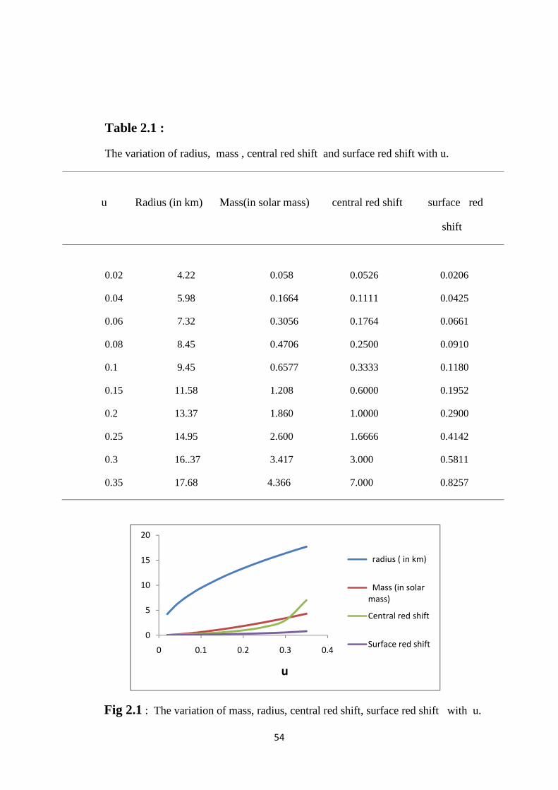
54
Table 2.1 :
The variation of radius, mass , central red shift and surface red shift with u.
u Radius (in km) Mass(in solar mass) central red shift surface red
shift
0.02 4.22 0.058 0.0526 0.0206
0.04 5.98 0.1664 0.1111 0.0425
0.06 7.32 0.3056 0.1764 0.0661
0.08 8.45 0.4706 0.2500 0.0910
0.1 9.45 0.6577 0.3333 0.1180
0.15 11.58 1.208 0.6000 0.1952
0.2 13.37 1.860 1.0000 0.2900
0.25 14.95 2.600 1.6666 0.4142
0.3 16..37 3.417 3.000 0.5811
0.35 17.68 4.366 7.000 0.8257
Fig 2.1 : The variation of mass, radius, central red shift, surface red shift with u.
0
5
10
15
20
0 0.1 0.2 0.3 0.4
u
radius ( in km)
Mass (in solarmass)
Central red shift
Surface red shift
55
2.4 Results and Discussions :
The solution obtained here is important because it is non-singular and
corresponds to infinite central density and pressure. Although the pressure and
density are infinite at the centre, but the red shift is finite. This solution is
important to study those stages of stellar evolution when the stellar object tends to
attain infinite pressure and infinite energy density. It would be possible to get the
information of these extreme stages of stellar evolution . Table 2.1 shows the
values of different parameters of Neutron star corresponding to different values of
u.The variation of mass, radius, central red shift and surface red shift with u has
been shown in the Fig 2.1. It has been observed that radius, mass, central red shift,
surface red shift increase with u. Central red shift increases more rapidly as
compared to the surface red shift. Eqs. (2.9) and (2.15) show that pressure and
density become infinite at the centre. The maximum mass of the neutron star based
on this solution comes out to be 4.366 MΘ with radius 17.68 km.
56
Section B
Solution II : A NEW WELL BEHAVED EXACT SOLUTION IN
ISOTROPIC COORDINATE SYSTEM FOR PERFECT FLUID.
2.5 Introduction:Neutron stars and quark stars are assumed to be the state of perfect fluid
balls in a static equilibrium. Hence in order to study such astrophysical problems
in the framework of General Relativity, the static solutions of Einstein’s field
equations for perfect fluid balls are desired.
Few successful attempts have been made to obtain exact static solutions of
Einstein’s field equations for perfect fluid balls in isotropic coordinates [28-30].
The desirability to obtain new exact solutions in isotropic coordinates lies in the
fact that those solutions which have very complicated form in canonical
coordinates may assume simple form in isotropic coordinates. Thus one can
consider Einstein’s gravitational field equations for perfect fluid and get their
physically significant solutions. In this chapter we present a new physically
relevant exact solution of Einstein’s field equations in isotropic coordinates.
The properties and characteristics of enormous gravity objects like neutron
star, white Dwarf , Quark star yet not solved fully in terms of maximization of
mass, can easily and significantly be understood with the help of Einstein’s field
equations of General Relativity. A considerable number of known solutions [31]
of Einstein’s field equations are of finite central pressure and finite central density
which may be useful for the modeling of some stellar objects. These solutions are
of paramount importance with pioneer relevancy for describing interior of the
Neutron star, as the central parameters are completely defined. The solutions
obtained by Tolman IV [2], Adler[7], Heintz[32], Finch and Skea[33] etc. do not
satisfy the one of the well behaved condition i.e. adiabatic sound speed is not
monotonically decreasing. Delgaty- Lake also pointed out that only nine solutions
so far are regular and well behaved; out of which seven in curvature coordinates
(Tolman vii [2], Patvardhav –Vaidya[34], Mehra[17], Kuchowicz[35] , Matese-
Whitman[36] , Durgapal’s two solutions[37] ) and only two solutions (Nariai
[38],Goldman[39]) in isotropic coordinates. The two new well behaved solutions
in curvature coordinates have been explored by N. Pant[40] , Gupta-Maurya [41]

57
and a new well behaved solution in isotropic coordinates has been obtained by
Pant et al. [42]. In this chapter we also present a new solution in isotropic
coordinates which is not only well behaved but also simple in terms of
expressions of field and physical variables. keeping in view the well behaved
nature of the solution we have constructed the models for supermassive
astrophysical configurations.
2.6 Conditions for well behaved solution:
From the physical point of view, the mathematical solutions must satisfy certain
physical requirements to render them physically meaningful. The following
conditions or requirements have been accepted [31, 42] .
(i) The solution should be free from physical and geometrical singularities i.e. finite and
positive values of central pressure, central density and non zero positive values of e
and e .
(ii) The solution should have positive and monotonically decreasing expressions for
pressure and density ( andp ) with the increase of r. The solution should have
positive value of ratio of pressure-density and less than 1(weak energy condition) ,
less than 1/3 (strong energy condition) throughout within the star.
(iii) The solution should have positive and monotonically decreasing expression for fluid
parameter 2c
p
with the increase of r.
(iv) The solution should have positive and monotonically decreasing expression for
velocity of sound
d
dpwith the increase of r and causality condition should be
obeyed at the centre i.e. 12
dc
dp
(v) d
PdP , everywhere within the ball.
(vi) Adiabatic index
P
d
dP
d
dP
Pd
Pd
e
e log
log
For realistic matter 1
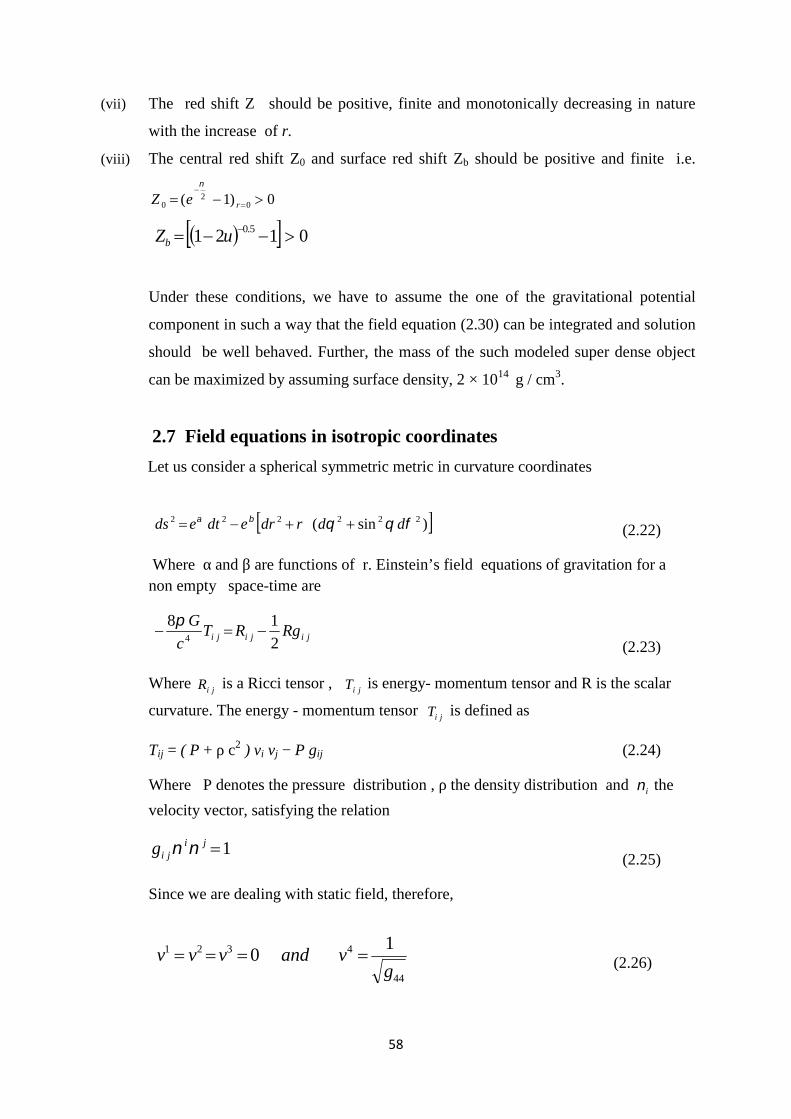
58
(vii) The red shift Z should be positive, finite and monotonically decreasing in nature
with the increase of r.
(viii) The central red shift Z0 and surface red shift Zb should be positive and finite i.e.
0)1( 02
0
reZ
0121 5.0 uZb
Under these conditions, we have to assume the one of the gravitational potential
component in such a way that the field equation (2.30) can be integrated and solution
should be well behaved. Further, the mass of the such modeled super dense object
can be maximized by assuming surface density, 2 × 10¹⁴ g / cm3.
2.7 Field equations in isotropic coordinates
Let us consider a spherical symmetric metric in curvature coordinates
)sin( 222222 ddrdredteds (2.22)
Where α and β are functions of r. Einstein’s field equations of gravitation for anon empty space-time are
jijiji RgRTc
G
2
184
(2.23)
Where jiR is a Ricci tensor , jiT is energy- momentum tensor and R is the scalar
curvature. The energy - momentum tensor jiT is defined as
Tij = ( P + ρ c2 ) vi vj − P gij (2.24)
Where P denotes the pressure distribution , ρ the density distribution and i the
velocity vector, satisfying the relation
1jijig
(2.25)
Since we are dealing with static field, therefore,
(2.26)44
4321 10
gvandvvv
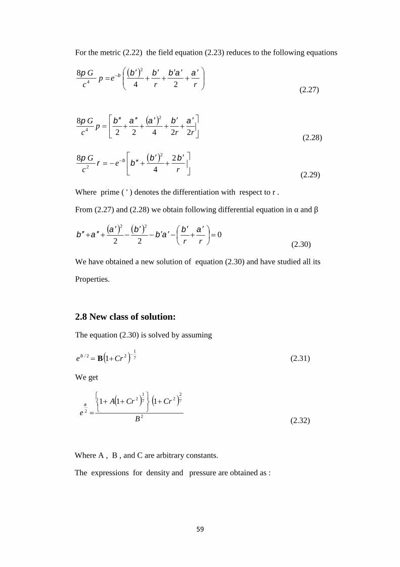
59
For the metric (2.22) the field equation (2.23) reduces to the following equations
rrep
c
G
24
8 2
4
(2.27)
rr
pc
G
22422
8 2
4
(2.28)
re
c
G
2
4
8 2
2
(2.29)
Where prime ( ' ) denotes the differentiation with respect to r .
From (2.27) and (2.28) we obtain following differential equation in α and β
0
22
22
rr
(2.30)
We have obtained a new solution of equation (2.30) and have studied all its
Properties.
2.8 New class of solution:
The equation (2.30) is solved by assuming
7
122/ 1
Cre B (2.31)
We get
2
7
227
12
2
111
B
CrCrA
e
(2.32)
Where A , B , and C are arbitrary constants.
The expressions for density and pressure are obtained as :

60
22
7
1222
2621
149
48rCC
CrBc
G
(2.33)
7
12
227
12
22
7
1222
4
)1(1
)75()1()47(
)1(49
48
CrA
CrCCrArCC
CrBc
pG
(2.34)
2.9 Properties of the new solution:
The central values of pressure and density are given by
A
ACC
Bc
pG
1
77
49
482
04
(2.35)
20
2 7
128
B
C
c
G
(2.36)
The central values of pressure and density will be non zero positive definite, if the
following conditions will be satisfied.
A > - 1/2, C > 0 (2.37)
Subjecting the condition that positive value of ratio of pressure-density and less than
1 at the centre i.e. 12
0
0 c
p
which leads to the following inequality,
11
13
1
A
A(2.38)
All the values of A which satisfy equation (2.37) , will also lead to the condition
.12
0
0 c
p
Differentiating (2.34) with respect to r,
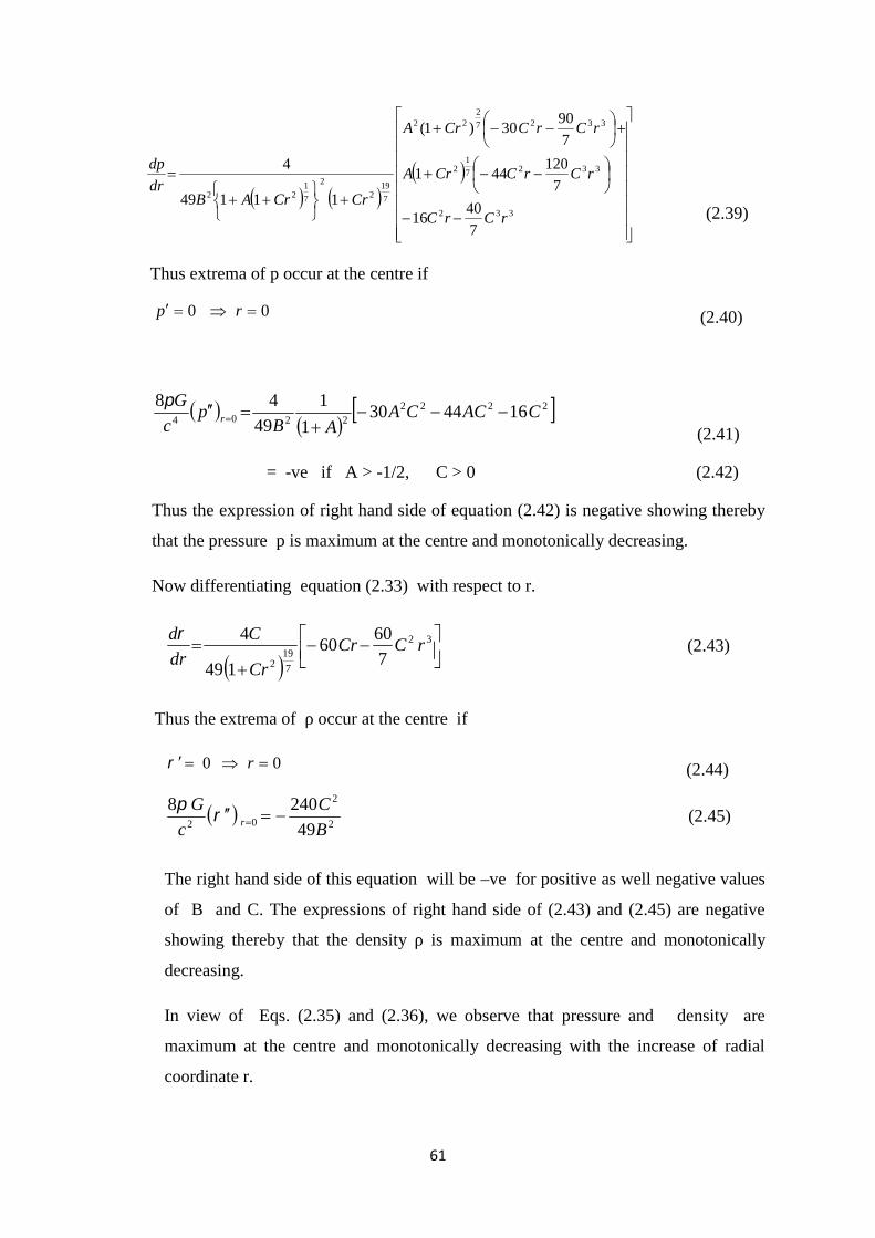
61
332
3327
12
3327
222
7
192
2
7
122
7
4016
7
120441
7
9030)1(
11149
4
rCrC
rCrCCrA
rCrCCrA
CrCrABdr
dp
(2.39)
Thus extrema of p occur at the centre if
00 rp (2.40)
22222204
1644301
1
49
48CACCA
ABp
c
Gr
(2.41)
= -ve if A > -1/2, C > 0 (2.42)
Thus the expression of right hand side of equation (2.42) is negative showing thereby
that the pressure p is maximum at the centre and monotonically decreasing.
Now differentiating equation (2.33) with respect to r.
32
7
192 7
6060
149
4rCCr
Cr
C
dr
d(2.43)
Thus the extrema of ρ occur at the centre if
00 r (2.44)
2
2
02 49
2408
B
C
c
Gr
(2.45)
The right hand side of this equation will be –ve for positive as well negative values
of B and C. The expressions of right hand side of (2.43) and (2.45) are negative
showing thereby that the density ρ is maximum at the centre and monotonically
decreasing.
In view of Eqs. (2.35) and (2.36), we observe that pressure and density are
maximum at the centre and monotonically decreasing with the increase of radial
coordinate r.

62
The square of adiabatic sound speed at the centre,
02
1
rd
dp
c , is given by
30
82215
1
11 2
20
2
AA
Ad
dp
cr
(2.46)
)(1 veand (2.47)
If following condition will be satisfied
A > -1/2, C > 0 (2.48)
The causality condition is obeyed at the centre for all values of constants
satisfying (2.48).
Further, it is mentioned here that the boundary of the super dense star is established
only when -1/2 < A < 0 .
In view of (2.33) and (2.34 ) the ratio of pressure-density is given by
222
7
12
22222
2 621
11
75147
rCC
CrA
CrCCrArCC
c
p
(2.49)
Differentiating (2.49) with respect to r, we get ;
dr
d
c
p2
(2.51)
222
c
p where (2.52)
Where
7
12
22222
11
75147
CrA
CrCCrArCC
(2.53)

63
= 222 621 rCC (2.54)
A
ACCr 1
770 (2.55)
20 21Cr (2.56)
2
7
127
52
222
22
7
627
12
2
1117
752
8480
1117
8
CrACr
CrCCrA
CrC
CrCrA
ACrrC
dr
d
(2.57)
212 Crdr
d
(2.58)
222
2
7
127
52
52332523
7
627
12
33
2 )621(
111
3014714772
760
168168
111
84
rCC
CrACr
rCrCrCArCrCr
CrCrA
ACrC
c
p
(2.59)
Thus extrema of2c
p
occur at the centre if
002
r
c
p
(2.60)
Differentiating (2.59) w. r. t. r, we get
(2.61) 4
22
2
c
p

64
Where
dr
dand
22 (2.62)
212C (2.63)
98670756
11149
5887201260
11149
8
422
7
122
2
7
12
22
422
7
1327
12
22
rCCr
CrCrA
CA
rCrC
CrCrA
ACC
rCr
CrCrA
rCA75
11149
8 3
7
112
3
7
12
33
(2.64)
2222
20
1
2
1
128
A
CA
A
ACCr
(2.65)
20 12Cr (2.66)
vec
pr
02
provided A > -1/2 , C > 0 (2.67)
2.10 Boundary conditions:
The solutions so obtained are to be matched over the boundary with Schwarzschild’s
exterior solution;
222222
1
222
22 sin
21
21 dRdRdR
Rc
GMdtc
Rc
GMds
(2.68)
Where M is the mass of the ball as determined by the external observer and R is the
radial coordinate of the exterior region. The boundary conditions are that the first and
second fundamental forms are continuous over the boundary r = rb or equivalently R =
Rb.

65
Applying the boundary conditions we get the values of the arbitrary constants in terms of
Schwarzschild’s parametersbRc
GMu
2 and bR
In view of Eqs. (1.43) and (1.45) we obtain two values of constants A as follows:
7
1
22
1
7
1
2
1
2
1
22
1
1
121
2175
12171
121
C
ku
u
u
kuA
(2.69)
7
822
1
7
122
2
122
)1(7)21()1(6
)21(4)1(7
bbb
bb
CruuCrCr
uCrCruA
(2.70)
From equation (2.69) and (2.70) we obtain the value of k as
u
Cr
CruuCrCr
uCrCru
k
b
bbb
bb
21
11
)1(7)21()1(6
)21(4)1(7 2
7
822
1
7
122
2
122
(2.71)
whereb
b
r
Rk
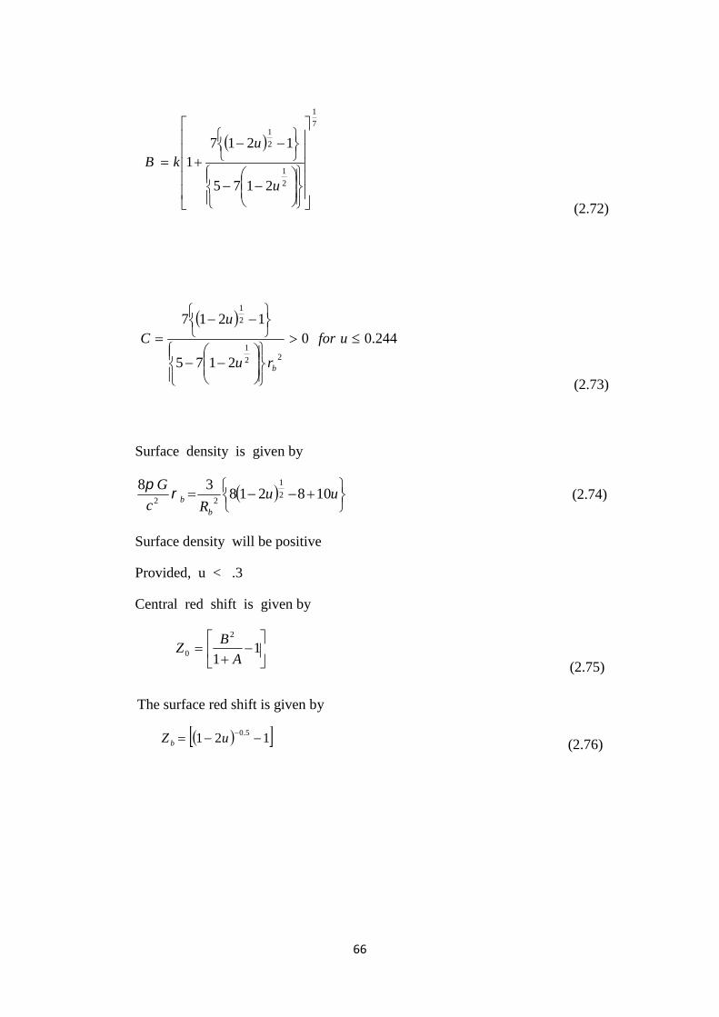
66
7
1
2
1
2
1
2175
12171
u
ukB
(2.72)
244.00
2175
1217
22
1
2
1
ufor
ru
uC
b
(2.73)
Surface density is given by
uu
Rc
G
b
b 10821838
2
1
22
(2.74)
Surface density will be positive
Provided, u < .3
Central red shift is given by
1
1
2
0 A
BZ
(2.75)
The surface red shift is given by
121 5.0 uZ b (2.76)
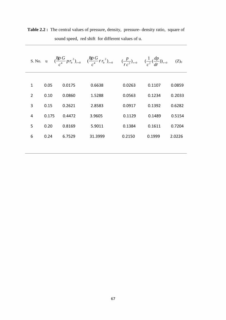
67
Table 2.2 : The central values of pressure, density, pressure- density ratio, square of
sound speed, red shift for different values of u.
S. No. u 02
4)
8( rbrp
c
G0
2
4)
8( rbrc
G
02
)( rc
p
02))(
1( rd
dp
c (Z)0
1 0.05 0.0175 0.6638 0.0263 0.1107 0.0859
2 0.10 0.0860 1.5288 0.0563 0.1234 0.2033
3 0.15 0.2621 2.8583 0.0917 0.1392 0.6282
4 0.175 0.4472 3.9605 0.1129 0.1489 0.5154
5 0.20 0.8169 5.9011 0.1384 0.1611 0.7204
6 0.24 6.7529 31.3999 0.2150 0.1999 2.0226

68
Table 2.3 : By assuming the surface density 314 /102 cmgb , the variation of
maximum Neutron star mass, radius Rb, central red shift Z0 and surface red shift
121 5.0 uZb with u . ( gmsunofMassM 33102 )
S. No. u 2
2
8bb r
c
G
M
MRb in km Z0 Zb
1 .01 0.1161 0.026 3.973 0.0153 0.0102
2 .02 0.2243 0.075 5.560 0.0315 0.0206
3 .04 0.4175 0.207 7.686 0.0667 0.0426
4 .06 0.5793 0.371 9.183 0.1063 0.066
5 .08 0.7100 0.556 10.318 0.1513 0.0911
6 .1 0.8094 0.754 11.190 0.2033 0.1180
7 .15 0.9229 1.262 12.479 0.3807 0.1953
8 .175 0.9084 1.498 12.688 0.5150 0.2401
9 .186 0.8874 1.591 12.685 0.5933 0.2618
Fig 2.2: The variation of radius (in km) with u .
02468
1012141618
0 0.05 0.1 0.15 0.2u
radius
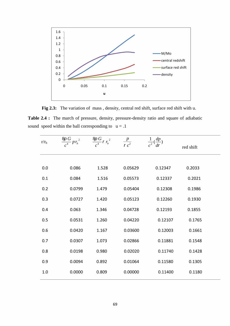
69
Fig 2.3: The variation of mass , density, central red shift, surface red shift with u.
Table 2.4 : The march of pressure, density, pressure-density ratio and square of adiabatic
sound speed within the ball corresponding to u = .1
r/rb2
4
8brp
c
G 2
4
8brc
G
2c
p
)(
12 d
dp
c red shift
0.0 0.086 1.528 0.05629 0.12347 0.2033
0.1 0.084 1.516 0.05573 0.12337 0.2021
0.2 0.0799 1.479 0.05404 0.12308 0.1986
0.3 0.0727 1.420 0.05123 0.12260 0.1930
0.4 0.063 1.346 0.04728 0.12193 0.1855
0.5 0.0531 1.260 0.04220 0.12107 0.1765
0.6 0.0420 1.167 0.03600 0.12003 0.1661
0.7 0.0307 1.073 0.02866 0.11881 0.1548
0.8 0.0198 0.980 0.02020 0.11740 0.1428
0.9 0.0094 0.892 0.01064 0.11580 0.1305
1.0 0.0000 0.809 0.00000 0.11400 0.1180
00.20.40.60.8
11.21.41.6
0 0.05 0.1 0.15 0.2
u
M/Mo
central redshift
surface red shift
density

70
Fig 2.4: The variation of p ,2c
p
, )(
12 d
dp
c, Z from centre to surface (u = 0.1)
Fig 2.5 : The variation of density from centre to surface (u = 0.1).
0
0.05
0.1
0.15
0.2
0.25
0 0.5 1 1.5
r/rb
pressure
pressure/density
d(pressure)/d(density)
red shift
0
0.2
0.4
0.6
0.8
1
1.2
1.4
1.6
1.8
0 0.2 0.4 0.6 0.8 1 1.2
r/rb
density

71
Table 2.5: The march of pressure, density, pressure-density ratio and square of adiabatic
sound speed within the ball corresponding to u = .06
r/rb2
4
8brp
c
G 2
4
8brc
G
2c
p
)(
12 d
dp
c red shift
0 0.026 0.816 0.0320 0.1131 0.1063
0.1 0.025 0.812 0.0317 0.1130 0.1058
0.2 0.024 0.803 0.0307 0.1128 0.1044
0.3 0.023 0.788 0.0291 0.1125 0.1021
0.4 0.020 0.767 0.0269 0.1121 0.0989
0.5 0.017 0.742 0.0240 0.1116 0.0949
0.6 0.014 0.713 0.0205 0.1109 0.0902
0.7 0.011 0.681 0.0163 0.1101 0.0848
0.8 0.007 0.648 0.0115 0.1093 0.0789
0.9 0.003 0.614 0.0060 0.1083 0.0726
1.0 0.000 0.579 0.0000 0.1072 0.0660

72
Fig 2.6: The variation of p ,2c
p
, z
d
dp
c,)(
12
from centre to surface for u = 0.06
Fig 2.7: The variation of density from centre to surface for u = 0.06
0
0.02
0.04
0.06
0.08
0.1
0.12
0 0.5 1 1.5
r/rb
pressure
pressure/density
d(pressure)/d(density)
red shift
00.10.20.30.40.50.60.70.80.9
0 0.2 0.4 0.6 0.8 1 1.2
r/rb
Density

73
Table 2.6: The march of pressure, density, pressure-density ratio, red shift and square
of adiabatic sound speed within the ball corresponding to u = .186
r/rb2
4
8brp
c
G 2
4
8brc
G
2c
p
)(
12 d
dp
c red shift
0 0.5745 4.654 0.1234 0.15394 0.5933
0.1 0.5482 4.483 0.1222 0.15393 0.5852
0.2 0.4790 4.033 0.1187 0.15388 0.5623
0.3 0.3882 3.443 0.1127 0.15377 0.5286
0.4 0.2962 2.844 0.1041 0.15353 0.4887
0.5 0.2147 2.313 0.0928 0.15307 0.4463
0.6 0.1479 1.876 0.0788 0. 15522 0.4044
0.7 0.0954 1.530 0.0623 0.15107 0.3644
0.8 0.0549 1.260 0.0435 0.14930 0.3271
0.9 0.0238 1.050 0.0226 0.14700 0.2929
1.0 0.0000 0.8874 0.0000 0.14410 0.2618

74
Fig 2.8: The variation of p , ,2c
p
, )(
12 d
dp
cfrom centre to surface for
u = 0.186.
2.11: Slowly rotating structures (Crab and the Vela Pulsars):
For slowly rotating structures like the Vela pulsars (rotation velocity
about 70 rad /sec), and the Crab pulsars (rotation velocity about 188 rad/sec)
one can calculate the moment of inertia in the first-order approximation which
appears in the Lense-Thrirring frame dragging effect. However, for the present
case of an exact solution, it is very useful to apply an approximate, but very
precise, empirical formula which is based on the numerical results obtained for
a large number of theoretical equations of state (EOS) of dense nuclear matter.
For the type of solution considered in the present study, the formula yields in
the following form [43-44].
I =(2/5)(1+x) MR2 ; (2.78)
where x is the dimensionless compactness parameter measured in units of
M (in km)/km, i.e.
x = (M/R)/MΘ (in km) km-1 (2.79)
Equation (2.78) is used to calculate the moment of inertia for the models
presented in Table 2.3 .
00.5
11.5
22.5
33.5
44.5
5
0 0.2 0.4 0.6 0.8 1
r/rb
pressure
density
pressure/density
d(pressure)/d(density)
red shift
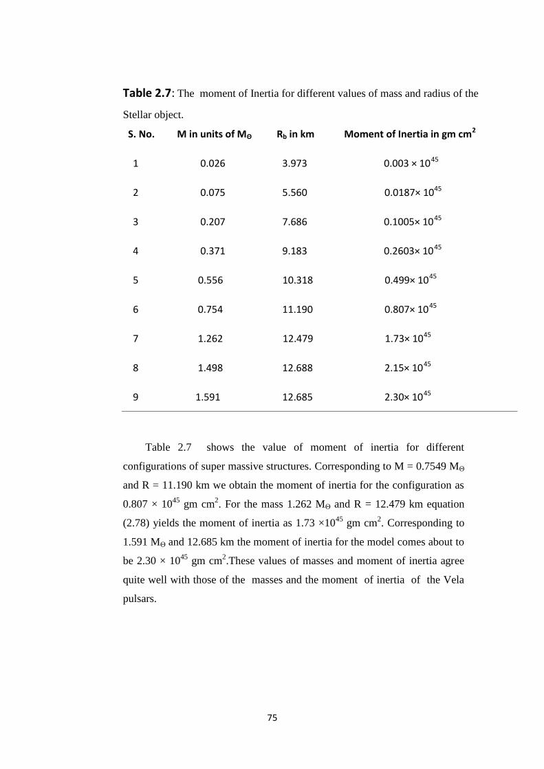
75
Table 2.7: The moment of Inertia for different values of mass and radius of the
Stellar object.
S. No. M in units of MΘ Rb in km Moment of Inertia in gm cm2
1 0.026 3.973 0.003 × 1045
2 0.075 5.560 0.0187× 1045
3 0.207 7.686 0.1005× 1045
4 0.371 9.183 0.2603× 1045
5 0.556 10.318 0.499× 1045
6 0.754 11.190 0.807× 1045
7 1.262 12.479 1.73× 1045
8 1.498 12.688 2.15× 1045
9 1.591 12.685 2.30× 1045
Table 2.7 shows the value of moment of inertia for different
configurations of super massive structures. Corresponding to M = 0.7549 MΘ
and R = 11.190 km we obtain the moment of inertia for the configuration as
0.807 × 1045 gm cm2. For the mass 1.262 MΘ and R = 12.479 km equation
(2.78) yields the moment of inertia as 1.73 ×1045 gm cm2. Corresponding to
1.591 MΘ and 12.685 km the moment of inertia for the model comes about to
be 2.30 × 1045 gm cm2.These values of masses and moment of inertia agree
quite well with those of the masses and the moment of inertia of the Vela
pulsars.
76
2.12 Results and Discussions :
The density of the massive fluid sphere is positive upto the value of u = .3, beyond
this value of u the density becomes negative. Hence we are restricted to the values of u less
than .3. From Table 2.3 we observe that linear dimension, mass and density of the stellar
object firstly increases with u upto u = .175 and then decreases. Central red shift and
surface red shift are positive within the stellar object and increases with increasing values of
u. The behaviour of all the parameters is well behaved and realistic only upto the value of
u = .186 . Beyond this value of u although the behaviour of all the parameters is well behaved
but the behaviour ofdc
dp2
is not normal,dc
dp2 firstly increases and then decreases as we go
from centre to surface or we can say that the trend of adiabatic sound speed is erratic. Thus
the solution is well behaved for all values of u satisfying the inequality 0 < u <0.186.
From the Table 2.4 and Table 2.5, we observe that the pressure and density are
positive and monotonically decreasing with the increase of radial coordinate r. The fluid
parameters2c
p
, )(
12 d
dp
care positive and monotonically decreasing with the increase of r.
Since )(1
2 d
dp
cis positive and less than 1 hence the causality condition is obeyed everywhere
within the ball . We now here present a model of super dense star based on the particular
solution discussed above by assuming surface density ; 2 × 10¹⁴ g / cm3 . Corresponding to u
= 0.186, the resulting well behaved model has maximum mass M = 1.591MΘ with radius Rb =
12.685 km. The model has mass within the range of neutron star. The good matching of our
results for Vela pulsars shows the robustness of our model.

77
2.13 References :
[1] Schwarzschild K.: “ On the Gravitational Field of a Mass Point
According to Einstein's Theory”, Sitzer. Preuss. Akad. Wiss. Berlin , pp.
189 (1916).
[2] Tolman, R.C.: “Static solutions of Einstein’s field equations for
spheres of fluid”, Phys. Rev. 55, 364(1939).
[3] Negi P. S. and Durgapal, M. C.: “Motion of test particles in
parabolic density distributions”, Astrophys. & Space Science 245, 97
(1996).
[4] Negi P. S. and Durgapal,M.C.: “Stable ultracompact objects”, Gen.
Rel. Grav. , 31, 13(1999).
[5] Durgapal, M. C.: “A class of new exact solutions in relativity”, J.
Phys. A. Math. Gen. 15, 2637 (1982).
[6] Durgapal, M. C. and Fuloria, R. S.: “Analytic stellar model for super-
dense star”, Gen. Rel. Grav. 17, 671(1985).
[7] Adlar, R. J. : “A fluid sphere in general relativity ”, J. Math. Phys.
15, 727(1974) .
[8] Adams, R. C. and Cohen, J. M.: “Analytic stellar models in general
relativity”,Astrophys & Space Sci. 198, 507(1975).
[9] Kuchowicz, B.: “A Physically Realistic Sphere of Perfect Fluid to
Serve as a Model of Neutron Stars”, Astrophys. & Space Sci. 131,
33 (1975).
[10] Buchdahl, H. A. : “General-Relativistic Fluid Spheres. III. a Static
Gaseous Model”, Astrophys. J. 147, 310 (1967).

78
.
[11] Vaidya, P. C. and Tikekar, R.: “Exact relativistic model for a
superdense star” J. Astrophys. & Astron. 3, 325(1982).
[12] Durgapal, M. C. and Bannerji, R.: “A new analytical stellar model
in general relativity”, Phys. Rev. D 27, 328(1983) . Erratum D28,
2695.
[13] Durgapal, M. C. and Rawat, P. S. : “Non-rigid spheres in general
relativity”, Mon. Not. R. Astr. Soc. 192, 659(1980).
[14] Buchdahl , H. A. : “A relativistic fluid sphere resembling the
Polytrope of index 5”, Ap. J. 140, 1512 (1964).
[15] Kuchowicz, B.: “General Relativistic fluid spheres. II. Solutions of
the equation for e ”,Acta Physica Polonica 34, 131(1968c).
[16] Leibovitz, C.: “Spherically Symmetric Static Solutions of Einstein's
Equations”, Phy. Rev.D 85,1664 (1969).
[17] Mehra A. L. : “Radially symmetric distribution of matter” , J.Aust.
Math. Soc. 6, 153 (1966).
[18] Pant, D. N. and Pant, N.: “A new class of exact solutions in general
relativity representing perfect fluid balls”, Journal of Mathematical
Physics 34, 2440(1993).
[19] Pant, D. N. : “Varieties of new classes of interior solutions in general
relativity ”, Astrophysics and Space Science, 215( 1), 97(1994).
[20] Pant, N.: “Uniform radial motion of sound in a relativistic fluid
ball”, Astrophysics and Space Science 240, 187 (1996).
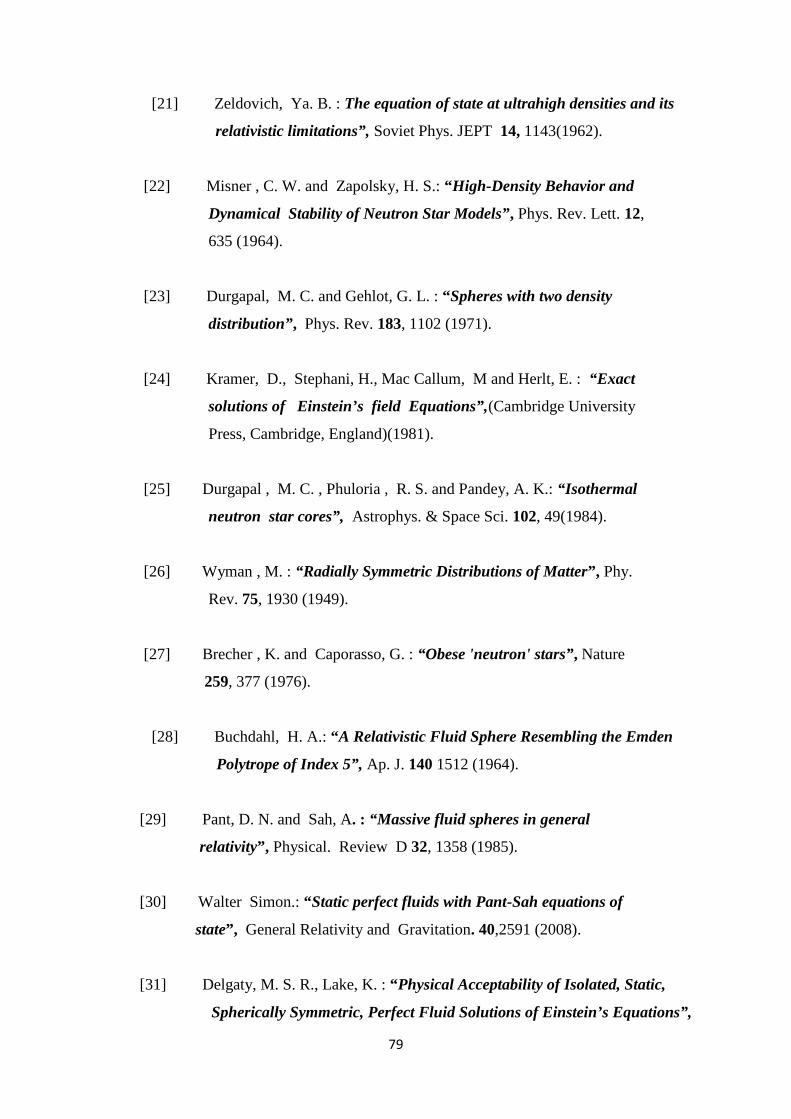
79
[21] Zeldovich, Ya. B. : The equation of state at ultrahigh densities and its
relativistic limitations”, Soviet Phys. JEPT 14, 1143(1962).
[22] Misner , C. W. and Zapolsky, H. S.: “High-Density Behavior and
Dynamical Stability of Neutron Star Models”, Phys. Rev. Lett. 12,
635 (1964).
[23] Durgapal, M. C. and Gehlot, G. L. : “Spheres with two density
distribution”, Phys. Rev. 183, 1102 (1971).
[24] Kramer, D., Stephani, H., Mac Callum, M and Herlt, E. : “Exact
solutions of Einstein’s field Equations”,(Cambridge University
Press, Cambridge, England)(1981).
[25] Durgapal , M. C. , Phuloria , R. S. and Pandey, A. K.: “Isothermal
neutron star cores”, Astrophys. & Space Sci. 102, 49(1984).
[26] Wyman , M. : “Radially Symmetric Distributions of Matter”, Phy.
Rev. 75, 1930 (1949).
[27] Brecher , K. and Caporasso, G. : “Obese 'neutron' stars”, Nature
259, 377 (1976).
[28] Buchdahl, H. A.: “A Relativistic Fluid Sphere Resembling the Emden
Polytrope of Index 5”, Ap. J. 140 1512 (1964).
[29] Pant, D. N. and Sah, A. : “Massive fluid spheres in general
relativity”, Physical. Review D 32, 1358 (1985).
[30] Walter Simon.: “Static perfect fluids with Pant-Sah equations of
state”, General Relativity and Gravitation. 40,2591 (2008).
[31] Delgaty, M. S. R., Lake, K. : “Physical Acceptability of Isolated, Static,
Spherically Symmetric, Perfect Fluid Solutions of Einstein’s Equations”,

80
Comput. Phys. Commun.115, 395 (1998).
[32] Heintzmann, H.: “New exact static solutions of Einsteins field
equations”, Z. Phys. 228, 489(1969).
[33] Finch , Skea: “A realistic stellar model based on an ansatz of Duorah
and Ray” , Class. Quan. Gravity 4, 467(1989).
[34] Patvardhav –Vaidya: J. Univ. Bombay 12, PartIII, 23(1943).
[35] Kuchowicz, B.: “General relativistic fluid spheres. II. Solutions of the
equation for e ”, Acta Phys. Pol 34 ,131(1968b).
[36] Matese-Whitman: “New method for extracting static equilibrium
configurations in general relativity”, Phys. Rev. D 22, 1270 (1980).
[37] Durgapal, M. C.: “A class of new exact solutions in relativity”, J.
Phys. A. Math. Gen. 15, 2637 (1980).
[38] Nariai H. : “On some static solutions of Einstein's gravitational field
equations in a spherically symmetric case”, Sci. Rep Tohoku Univ Serl
34,160 (1950).
[39] Goldman, S. P.: “Physical solutions to general-relativistic fluid
spheres”, Astrophys J. 226 1079(1978).
[40] Pant, N.: “Some new exact solutions with finite central parameters and
uniform radial motion of sound ”, Astrophys. Space Sci. 331, 633
(2011).
[41] Maurya, S.K., Gupta, Y.K.: “On a family of well behaved perfect fluid
balls as astrophysical objects in general relativity”, Astrophys Space
Sci.334(1),145 (2011).

81
[42] Pant, N. et al.: “New class of regular and well behaved exact solution
in general relativity”, Astrophys. Space Sci. 330, 353(2010).
[43] Bejger, M., Haensal, P. : “Moments of inertia for neutron and strange
stars Limits derived for the Crab pulsar”, Astron. Astrophys. 396 917
(2002).
[44] Pant N. , Negi P.S.: “Variety of well behaved exact solutions of
Einstein– Maxwell field equations, an application to Strange Quark
stars, Neutron stars and Pulsars”, Astrophys Space Sci ,338 (1), 163
(2012).
Chapter IIIA Parametric class of Regularand well behaved relativistic
Charged fluid spheres

82
Chapter III
A Parametric class of Regular and well behaved
relativistic Charged fluid spheres3
In this chapter we have studied well behaved parametric class of charge
Analogue of Durgapal’s V solution [1]. We have obtained a generalized solution of
Einstein-Maxwell field equations of general relativity for a charged , static,
spherically symmetric fluid ball. We present charged super-dense star models after
prescribing particular forms of the metric potential and electric intensity. The metric
describing the super dense stars joins smoothly with the Reissner-Nordstrom metric
at the pressure free boundary. The electric density assumed is
3
2
2
21
1
2
)61()1(2
xxKx
x
qc
c
E n where n may take the values 0 ,1, 2, 3, 4 and so on
and K is a positive parameter. For n = 0 we rediscovered the Gupta, Maurya
solution [2]. For n = 1 we get the Fuloria, et al. solution [3]. The solution for n =
1, n = 2 and n = 3 have been discussed extensively keeping in view of well behaved
nature of the charged solution of Einstein–Maxwell field equations.
3 Some part of this chapter has been published in J. Modern physics, 2,(10)1156 (2011) & Another part has been published in Astrophysics & SpaceScience, 341,469 (2012).
83
3.1 Introduction:
Exact solutions with well-behaved nature of Einstein-Maxwell field equations
are of great interest in relativistic astrophysics. Such solutions may be used to make a
suitable model of super dense object with charge matter like Neutron star, quark star,
pulsar and analogous stars. It is interesting to observe that, in the presence of charge,
the gravitational collapse of a spherical symmetric distribution of the matter to a
point singularity may be avoided because the presence of some charge in a spherical
material distribution provides an additional resistance against the gravitational
contraction by means of electric repulsion. The inclusion of charge plays very
important role in the stability of massive fluid spheres. A spherical fluid
distribution of uniform density with a net charge on the surface is more stable than a
surface without charge[4,5] . According to De Felice et al.[6] the inclusion of charge
inhibits the growth of space time curvature and which therefore plays a key role in
avoiding singularities. Thus a stable massive charged configuration can be produced
in which repulsive force from the charge counter balances the gravitational attraction.
The singularities which appear in the Schwarzschild solution corresponding to
spherically symmetric static perfect fluid distribution can be avoided to a great extent
by including charge in them. The negative pressure of Bayin’s solution[7] makes it
physically unreasonable, however the inclusion of charge in Bayin’ solution makes it
physically reasonable i.e. the pressure is a decreasing function of radius from centre
to surface (Ray et al.) [8] . Bonner [9] has shown that dust cloud of arbitrarily large
mass and small radius can remain in equilibrium if it has an electric charge density
related to the mass density by . All these advantages of charged spherical
models motivated us to consider the charge analogue of Durgapal’ solution[1].
To include the electric charge a number of authors make additional assumptions
such as an equation of state or a relationship between metric variables [10-13].
Bonnor and Wickramasuriya [14] have studied electrically charged matter, with
electrostatic repulsion balancing the gravitational attraction. Most works have been
done under static conditions, including the ones by Ivanov [15], who exhaustively
surveyed static charged perfect fluid spheres in general relativity, and Ray et al. [16],
84
who studied the effect of electric charge in compact stars and its consequences on the
gravitational collapse. Bekenstein [17] found that for highly relativistic stars, whose
radius is on the verge of forming an event horizon, the large gravitational pull can be
balanced by large amounts of net charge.
The Reissner-Nordstrom solution for the external field of a charged fluid
sphere has two distinct singularities at finite radial positions unlike Schwarzschild
solution which has the singularity at the centre also. Thus the Reissner-Nordstrom
solution describes the bridge between two asymptotically flat spaces and an electric
flux flowing across the bridge. Graves and Brill [18] pointed out that the region of
minimum radius pulsates periodically between these two surfaces due to Maxwell
pressure of the electric field. Thus the study of charged fluid spheres is important
due to having many important implications. Many Exact solutions of Einstein’s field
equations which are not well behaved and regular become well behaved after
including charge in them. A classical model of an electron may be represented by
charged dust if most of its characteristics remain finite and non- trivial while the
junction radius shrinks to zero. Ray and Das[19] , Bonner and Cooperstock [20]
have assumed that charged fluid balls with electromagnetic mass may be used to
depict the model of an electron.
On account of the non linearity of Einstein Maxwell field equations , not many
realistic well behaved, analytic solutions are known for the description of charged
fluid spheres. Astrophysicists have been using exact solutions of Einstein’s field
equations as seed solutions for the modeling of charged fluid spheres. Bonnor [21],
Efinger [22], Kyle and Martin [23], Krori and Barua [24] and Nduka [25] have
obtained internal solutions for static spherically symmetric charged fluid spheres
under different conditions.
Our aim is also to find a new parametric class of exact solutions of Einstein–
Maxwell field equations for a static, spherically symmetric distribution of the
charged and perfect fluid with well behaved nature and to construct suitable models
of super dense objects with charge matter. Many of the authors electrified the well
known uncharged fluid spheres e.g. Durgapal-Fuloria solution [26] by Gupta and
Maurya [27], Schwarzschild solution [28] by Bijalwan and Gupta [29] and by Gupta
and Kumar [30], Kuchowicz solution [31] by Nduka[32] , Tolman solution [33] by
Cataldo and Mitskievic [34], Heintzmann’s solution [35] by Pant et al. [36] , Adler’s
solution by Pant et al.[37] and M. J. Pant andTewari [38] and so on. These coupled

85
solutions are well behaved with some positive values of charge parameter K and
completely describe interior of the super-dense stellar objects with charge matter.
We have tried to charge the Durgapal’s V solution [1] after prescribing
particular forms of metric potential g44 and electric intensity .Some new solutions of
Einstein’s Maxwell field equations have been obtained keeping in view their well
behaved nature. Models of super massive charged fluid spheres have been
constructed by working out new solutions of Einstein’s Maxwell Field Equations.
3.2 The solutions that are used as seed solutions for making
charged fluid model:
The solutions that may be used as seed solutions for the construction of charged
fluid models may be categorized as follows:[39]
Type I : If the solutions are well behaved; such solutions may be used to describe
the interior of super massive stellar objects and may be used as seed solutions for
constructing relativistic charged fluid ball models. Such charged solutions and their
neutral counterparts both show well behaved nature and regularity .
Type II : If the solutions are not well behaved, but with finite parameters; such
solutions may be taken as seed solutions of super dense star with charge matter,
Schwarzschild’s interior solution is not well behaved as causality condition is not
obeyed throughout within the fluid sphere. However, charge analogues of the
solution are well behaved for wide range of constants (Gupta and kumar [30];
Bijalwan, N. and Gupta [29]; Florides [40] ). Adler solution[41] and Durgapal and
Fuloria solution [26] are also not well behaved as the speed of sound is
monotonically increasing from centre to boundary. However, charge Analogues of
the solution is well behaved for wide range of constants [42]. Heintzmann’s neutral
solution [35] is not well behaved as the speed of sound is monotonically increasing
from centre to boundary . However the charge analogue of solution is well behaved
for wide range of constant [36].

86
3.3 Assumptions that must be satisfied in order for the solution to
be well behaved [43-44]:
(i) The solution should be free from physical and geometrical singularities i.e. finite and
positive values of central pressure , central density i.e. p0 > 0 and ρ0 > 0 and non
zero positive values of e and e . For such solutions the tangent 3-space at the centre
is flat and it is an essential condition. For curvature coordinates, mathematically it is
expressed as 10
re and 0re positive constant[45-46].
(ii) The solution should have positive and monotonically decreasing expressions for
pressure and density( andp )with the increase of r. i.e.
(a) pandpandrp r 000 0 is negative valued function for r > 0.
(b) andandr r 000 0 is negative valued function for r > 0.
(iii) The solution should have positive value of ratio of pressure-density and less than 1
with in the ball i. e. 102
c
p
.
(iv) The solution should have positive and monotonically decreasing expression for
fluid parameter 2c
p
with the increase of r .
(v) The solution should have positive and monotonically decreasing expression for
velocity of sound
d
dpwith the increase of r and causality condition should be
obeyed at the centre i.e. 12
dc
dp.
(vi) The central red shift Z0 and surface red shift Zb should be positive and finite i.e.
010
20
r
eZ
and 012
b
eZb
and both should be bounded and
monotonically decreasing in nature with the increase of r i.e. 00
rdr
dz
(vii) Electric intensity E is positive and monotonically increasing from centre to
boundary and at the centre the electric intensity is zero.
(viii) The pressure at the boundary should be zero.
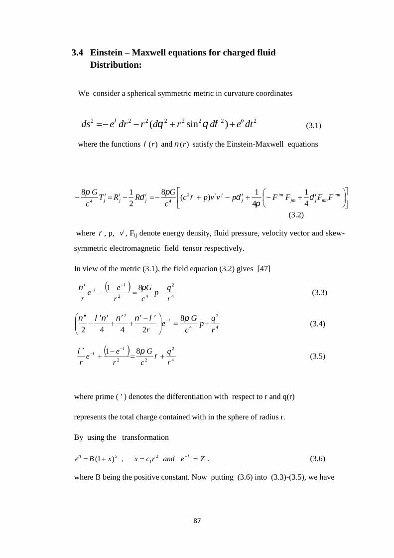
87
3.4 Einstein – Maxwell equations for charged fluidDistribution:
We consider a spherical symmetric metric in curvature coordinates
22222222 )sin( dtedrdrdreds (3.1)
where the functions )(r and )(r satisfy the Einstein-Maxwell equations
mn
mnijjm
imij
jiij
ij
ij FFFFpvvpc
c
GRRT
c
G
4
1
4
1)(
8
2
18 244
(3.2)
where , p, iv , Fij denote energy density, fluid pressure, velocity vector and skew-
symmetric electromagnetic field tensor respectively.
In view of the metric (3.1), the field equation (3.2) gives [47]
4
2
42
81
r
qp
c
G
r
ee
r
(3.3)
4
2
4
2 8
2442 r
qp
c
Ge
r
(3.4)
4
2
22
81
r
q
c
G
r
ee
r
(3.5)
where prime ( ' ) denotes the differentiation with respect to r and q(r)
represents the total charge contained with in the sphere of radius r.
By using the transformation
ZeandrcxxBe 21
5 ,)1( . (3.6)
where B being the positive constant. Now putting (3.6) into (3.3)-(3.5), we have

88
41
2
21 81)1(
)1(
10
c
PG
cx
qc
x
Z
x
Z
(3.7)
41
2
21 81
2)1(
c
G
cx
qc
dX
dZ
x
Z
(3.8)
and Z satisfying the equation
)61(
)1(1)/2(
)61(1
1214 122
xx
xxcqZ
xxxx
xx
dx
dZ
(3.9)
3.5 A New Generalised solution of Einstein-Maxwell Field
Equations:
In order to solve the differential equation (3.9) we consider the electric intensity E
of the following form
3
2
2
21
1
2
)61()1(2
xxKx
x
qc
c
E n (3.10)
where K is a positive constant. The electric density is so assumed that the model is
physically significant and well behaved i.e. E remains regular and positive
throughout the sphere.
In view of (3.10) differential equation (3.9) yields the following solution:
3
3
1
2
33/1
2
)1(
)61(112
)854309(1
)1(
1
)61(
)1(
)5(x
x
Axxxx
xx
xx
n
KZ
n
(3.11)
where A is an arbitrary constant of integration.
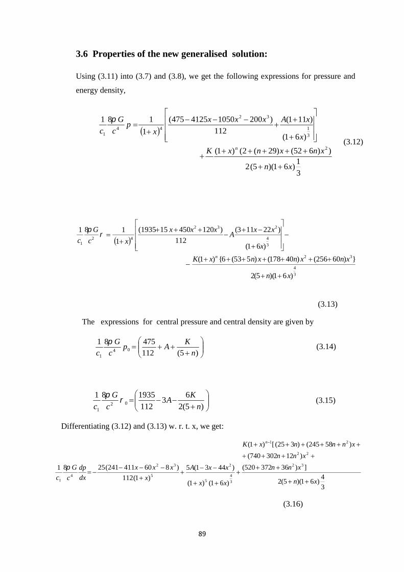
89
3.6 Properties of the new generalised solution:
Using (3.11) into (3.7) and (3.8), we get the following expressions for pressure and
energy density,
3
1)61)(5(2
))652()29(2()1(
)61(
)111(
112
)20010504125475(
1
181
2
3
1
32
441
xn
xnxnxK
x
xAxxx
xp
c
G
c
n
(3.12)
3
4
32
3
4
232
421
)61)(5(2
})60256()40178()553(6{)1(
)61(
)22113(
112
)120450151935(
1
181
xn
xnxnxnxK
x
xxA
xxx
xc
G
c
n
(3.13)
The expressions for central pressure and central density are given by
)5(112
4758104
1 n
KAp
c
G
c
(3.14)
)5(2
63
112
19358102
1 n
KA
c
G
c
(3.15)
Differentiating (3.12) and (3.13) w. r. t. x, we get:
3
4)61)(5(2
])36372520(
)12302740(
)58245()325([)1(
)61()1(
)4431(5
)1(112
)860411241(2581 32
22
21
3
45
2
5
32
41 xn
xnn
xnn
xnnnxK
xx
xxA
x
xxx
dx
dp
c
G
c
n
(3.16)
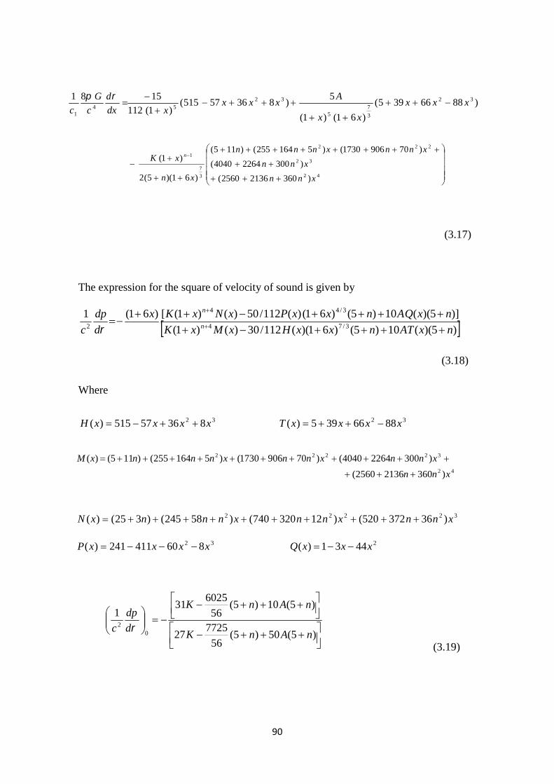
90
)8866395(
)61()1(
5)83657515(
)1(112
1581 32
3
75
3254
1
xxx
xx
Axxx
xdx
d
c
G
c
42
32
222
3
7
1
)36021362560(
)30022644040(
)709061730()5164255()115(
)61)(5(2
)1(
xnn
xnn
xnnxnnn
xn
xK n
(3.17)
The expression for the square of velocity of sound is given by
)5)((10)5()61)((112/30)()1(
)]5)((10)5()61()(112/50)()1([)61(13/74
3/44
2 nxATnxxHxMxK
nxQAnxxPxNxKx
d
dp
c n
n
(3.18)
Where
32 83657515)( xxxxH 32 8866395)( xxxxT
42
32222
)36021362560(
)30022644040()709061730()5164255()115()(
xnn
xnnxnnxnnnxM
32222 )36372520()12320740()58245()325()( xnnxnnxnnnxN
32 860411241)( xxxxP 24431)( xxxQ
)5(50)5(56
772527
)5(10)5(56
602531
1
02
nAnK
nAnK
d
dp
c
(3.19)
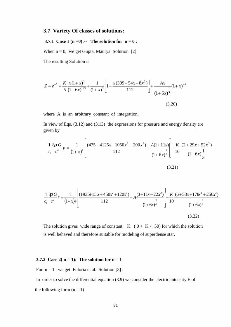
91
3.7 Variety Of classes of solutions:
3.7.1 Case 1 (n =0):-- The solution for n = 0 :
When n = 0, we get Gupta, Maurya Solution [2].
The resulting Solution is
3
3
1
2
33/1
2
)1(
)61(112
)854309(1
)1(
1
)61(
)1(
5
x
x
Axxxx
xx
xxKeZ
(3.20)
where A is an arbitrary constant of integration.
In view of Eqs. (3.12) and (3.13) the expressions for pressure and energy density aregiven by
3
1)61(
)52292(
10)61(
)111(
112
)20010504125475(
1
181 2
3
1
32
441 x
xxK
x
xAxxx
xp
c
G
c
(3.21)
3
4
32
3
4
232
21 )61(
)256178536(
10)61(
)22113(
112
)120450151935(
41
181
x
xxxK
x
xxA
xxx
xc
G
c
(3.22)
The solution gives wide range of constant K ( 0 < K 50) for which the solution
is well behaved and therefore suitable for modeling of superdense star.
3.7.2 Case 2( n = 1): The solution for n = 1
For n = 1 we get Fuloria et al. Solution [3] .
In order to solve the differential equation (3.9) we consider the electric intensity E of
the following form (n = 1)

92
3
2
2
21
1
2
)61()1(2
xxKx
x
qc
c
E (3.23)
where K is a positive constant. In view of equation (3.11) we get the following solution
3
3
1
2
33/1
3
)1(
)61(112
)854309(1
)1(
1
)61(
)1(
6x
x
Axxxx
xx
xxKe
(3.24)
where A is an arbitrary constant of integration.
3.8 Properties of the new solution for n = 1:
In view of Equations (3.12) and (3.13), we get the following expressions for pressure and
energy density
3
1)61(
)29151()1(
6)61(
)111(
112
)20010504125475(
1
181 2
3
1
32
441 x
xxxK
x
xAxxx
xp
c
G
c
(3.25)
3
4
32
3
4
232
21 )61(
)158109293()1(
6)61(
)22113(
112
)120450151935(
41
181
x
xxxxk
x
xxA
xxx
xc
G
c
(3.26)
The expressions for central pressure and central density are given by the
following equations:
6112
4758104
1
KAp
c
G
c
(3.27)
23
112
19358102
1
KA
c
G
c
(3.28)

93
In view of equations ( 3.16) and (3.17) we get:
3
4)61(6
)46452715214(
)61()1(
)4431(5
)1(112
)860411241(2581 32
3
45
2
5
32
41 x
xxxK
xx
xxA
x
xxx
dx
dp
c
G
c
(3.29)
432
3
7
32
3
75
3254
1
2528330213532128
)61(6
)8866395(
)61()1(
5)83657515(
)1(112
1581
xxxx
x
K
xxx
xx
Axxx
xdx
d
c
G
c
(3.30)
3
75
112
6025)
81( 04
1
KA
dx
dp
c
G
c
(3.31)
3
425
112
7725)
81( 04
1
KA
dx
d
c
G
c
(3.32)
The velocity of sound is given by the following expression:
53
7432
3
73232
53
432
3
4232
2
)1()61)(2528330213532128(30
112
)61)(8866395(112)83657515(3
)1()61)(46452715214(30
112
)61)(4431(112)860411241(5
1
xxxxxxK
xxxxAxxx
xxxxxK
xxxAxxx
d
dp
c
(3.33)
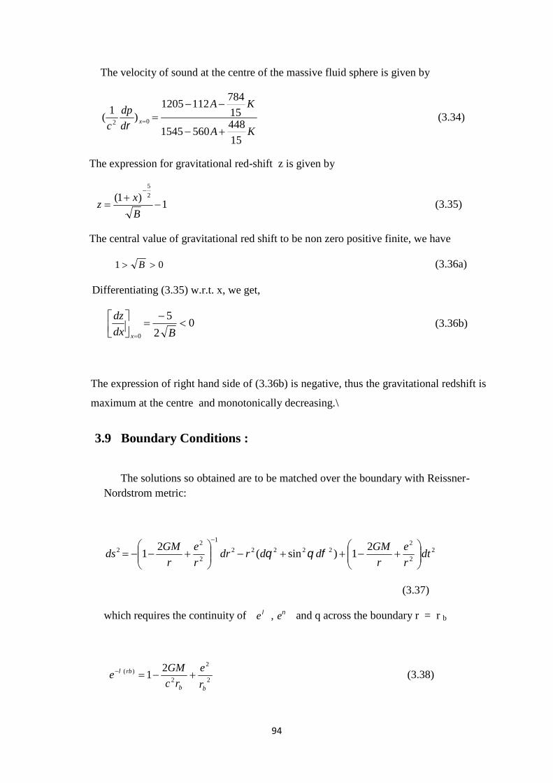
94
The velocity of sound at the centre of the massive fluid sphere is given by
KA
KA
d
dp
c x
15
4485601545
15
7841121205
)1
( 02
(3.34)
The expression for gravitational red-shift z is given by
1)1( 2
5
B
xz (3.35)
The central value of gravitational red shift to be non zero positive finite, we have
01 B (3.36a)
Differentiating (3.35) w.r.t. x, we get,
02
5
0
Bdx
dz
x
(3.36b)
The expression of right hand side of (3.36b) is negative, thus the gravitational redshift is
maximum at the centre and monotonically decreasing.\
3.9 Boundary Conditions :
The solutions so obtained are to be matched over the boundary with Reissner-Nordstrom metric:
22
222222
1
2
22 2
1)sin(2
1 dtr
e
r
GMddrdr
r
e
r
GMds
(3.37)
which requires the continuity of ee , and q across the boundary r = r b
2
2
2)( 2
1bb
rb
r
e
rc
GMe (3.38)
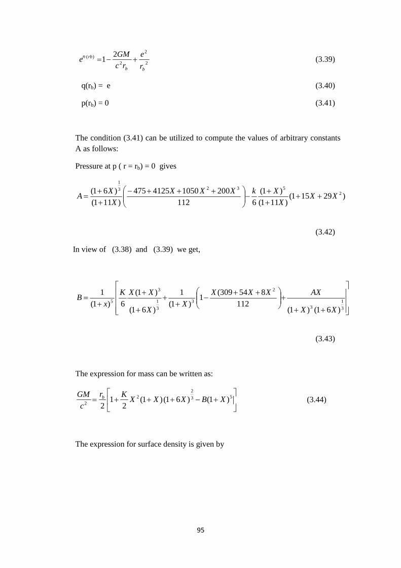
95
2
2
2)( 2
1bb
rb
r
e
rc
GMe (3.39)
q(rb) = e (3.40)
p(rb) = 0 (3.41)
The condition (3.41) can be utilized to compute the values of arbitrary constantsA as follows:
Pressure at p ( r = rb) = 0 gives
)29151()111(
)1(
6112
20010504125475
)111(
)61( 25323
1
XXX
XkXXX
X
XA
(3.42)
In view of (3.38) and (3.39) we get,
3
13
2
3
3
1
3
5
)61()1(112
854309(1
)1(
1
)61(
)1(
6)1(
1
XX
AXXXX
XX
XXK
xB
(3.43)
The expression for mass can be written as:
53
22
2)1()61()1(
21
2XBXXX
Kr
c
GM b (3.44)
The expression for surface density is given by

96
3
4
32
3
4
2322
2
)61(
)158109293()1(
6
)61(
)22113(
112
)120450151935(
41
18
X
XXXXK
X
XXA
XXX
Xr
c
Gbb
(3.45)
We have obtained the expressions for pressure, density, pressure-density ratio and
square of adiabatic sound speed within the charged fluid sphere for the solution n =1.
Now we study the variation of different physical quantities from centre to surface .
If pressure, density, pressure-density ratio , red shift would be positive within the
charged fluid sphere and monotonically decreasing from centre to surface ,then the
solution will be suitable for modeling of super massive charged fluid balls.
Table 3.1 : The variation of various physical parameters at the centre, surface density,electric field intensity on the boundary, mass and radius of stars with different values of Kand X = .2
K 041
81p
c
G
c
02
1
81
c
G
c 0
02
1
p
c 02)(
1xd
dp
c 0zbr
c
E
1
22
2
8bb r
c
G
M
Mbr
km
1 5.167 14.496 0.3565 0.9298 1.63 0.202 1.3728 4.41 19.20
2 4.664 16.0037 0.2914 0.7017 1.68 0.404 1.277 4.60 18.52
4 3.660 19.0156 0.1925 0.4806 1.814 0.808 1.060 4.83 16.87
5 3.158 20.5217 0.1538 0.4186 1.885 1.01 0.955 4.88 16.02
6 2.656 22.0275 0.1205 0.3728 1.962 1.212 0.851 4.89 15.12
8 1.652 25.0394 0.0659 0.3411 2.134 1.616 0.643 4.75 13.14
10 0.648 28.0513 0.0231 0.2655 2.342 2.02 0.434 4.31 10.80

97
Table 3.2 : The variation of various physical parameters at the centre, surface density,
electric field intensity on the boundary, mass and radius of stars with different values of X
and K = 2
X 041
81p
c
G
c
02
1
81
c
G
c 0
02
1
p
c 02)(
1xd
dp
c 0zbr
c
E
1
22
2
8bb r
c
G
M
Mbr
In km
.10 3.6036 19.1889 0.1889 0.5628 0.754 0.1504 1.181 2.95 17.81
.15 4.2883 17.1349 0.2502 0.6416 1.196 0.2646 1.282 3.89 18.55
.20 4.6643 16.0037 0.2914 0.7017 1.688 0.404 1.277 4.60 18.52
.25 4.8138 15.5583 0.3094 0.7300 2.276 0.5756 1.168 5.13 17.71
.30 4.764 15.7075 0.3032 0.7202 3.000 0.7747 0.989 5.50 16.29
.35 4.5018 16.4343 0.2751 0.6738 3.985 1.0045 0.7276 5.52 13.98

98
Table 3.3 : The variation of various physical parameters at the center, surface density, electric fieldintensity on the boundary, mass and radius of stars with different values of K and X = .1
_________________________________________________________________________________
K 041
81p
c
G
c
02
1
81
c
G
c 0
02
1
p
c 02)(
1xd
dp
c 0zbr
c
E
1
22
2
8bb r
c
G
M
Mbr in km
________________________________________________________________________________
1 3.79 18.61 0.2037 0.6366 0.760 0.075 1.200 2.95 17.95
2 3.60 19.18 0.1877 0.5628 0.766 0.150 1.181 2.99 17.81
3 3.22 20.32 0.1585 0.4542 0.780 0.300 1.142 3.08 17.51
4 3.03 20.89 0.1451 0.4131 0.787 0.376 1.122 3.12 17.36
5 2.84 21.46 0.1324 0.3781 0.794 0.451 1.103 3.16 17.21
6 2.46 22.60 0.1089 0.3210 0.808 0.601 1.064 3.23 16.90
8 2.08 23.74 0.0877 0.278 0.823 0.752 1.024 3.30 16.59
10 1.89 24.31 0.0778 0.260 0.830 0.827 1.005 3.33 16.43
12 1.70 24.88 0.0684 0.244 0.838 0.902 0.985 3.36 16.27
14 1.32 26.02 0.0594 0.216 0.853 1.053 0.946 3.42 15.94
16 0.94 27.16 0.0347 0.193 0.869 1.283 0.907 3.47 15.61
18 0.86 28.30 0.0199 0.173 0.885 1.354 0.868 3.51 15.27
20 0.184 29.44 0.0062 0.157 0.902 1.504 0.829 3.55 14.92

99
Table 3.4 : The variation of various physical parameters at the center, surface density, electricld intensity on the boundary, mass and radius of stars with different values of K and X =.01
K 041
81p
c
G
c
02
1
81
c
G
c 0
02
1
p
c 02)(
1xd
dp
c 0zbr
c
E
1
22
2
8bb r
c
G
M
Mbr
In km
2 0.653 28.03 0.0233 0.405 0.07479 0.010 0.2640 0.2565 8.422
4 0.623 28.13 0.0221 0.363 0.07485 0.021 0.2638 0.2569 8.418
6 0.592 28.22 0.0210 0.326 0.07491 0.031 0.2636 0.2574 8.415
8 0.562 28.31 0.0198 0.293 0.07496 0.042 0.2634 0.2579 8.411
10 0.531 28.40 0.0187 0.264 0.07502 0.052 0.2631 0.2583 8.407
12 0.501 28.49 0.0175 0.238 0.07510 0.063 0.2629 0.2588 8.404
14 0.470 28.58 0.0164 0.214 0.07514 0.073 0.2627 0.2592 8.400
16 0.440 28.67 0.0153 0.193 0.07516 0.084 0.2624 0.2596 8.396
20 0.379 28.86 0.0131 0.156 0.07533 0.105 0.2620 0.2606 8.389
30 0.226 29.32 0.0077 0.086 0.07550 0.157 0.2609 0.2629 8.371
40 0.073 29.78 0.0024 0.037 0.07581 0.210 0.2597 0.2651 8.353
44 0.012 29.96 0.0004 0.021 0.07598 0.231 0.2593 0.2660 8.345
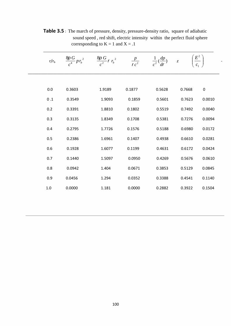
100
Table 3.5 : The march of pressure, density, pressure-density ratio, square of adiabatic
sound speed , red shift, electric intensity within the perfect fluid spherecorresponding to K = 1 and X = .1
_________________________________________________________________________
r/rb2
4
8brp
c
G 2
2
8brc
G
2c
p
)(
12 d
dp
cz
1
2
c
E-
__________________________________________________________________________________________
0.0 0.3603 1.9189 0.1877 0.5628 0.7668 0
0 .1 0.3549 1.9093 0.1859 0.5601 0.7623 0.0010
0.2 0.3391 1.8810 0.1802 0.5519 0.7492 0.0040
0.3 0.3135 1.8349 0.1708 0.5381 0.7276 0.0094
0.4 0.2795 1.7726 0.1576 0.5188 0.6980 0.0172
0.5 0.2386 1.6961 0.1407 0.4938 0.6610 0.0281
0.6 0.1928 1.6077 0.1199 0.4631 0.6172 0.0424
0.7 0.1440 1.5097 0.0950 0.4269 0.5676 0.0610
0.8 0.0942 1.404 0.0671 0.3853 0.5129 0.0845
0.9 0.0456 1.294 0.0352 0.3388 0.4541 0.1140
1.0 0.0000 1.181 0.0000 0.2882 0.3922 0.1504
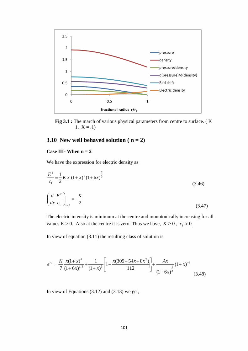
101
Fig 3.1 : The march of various physical parameters from centre to surface. ( K1, X = .1)
3.10 New well behaved solution ( n = 2)
Case III- When n = 2
We have the expression for electric density as
3
22
1
2
)61()1(2
1xxxK
c
E
(3.46)
201
2 K
c
E
dx
d
x
(3.47)
The electric intensity is minimum at the centre and monotonically increasing for all
values K > 0. Also at the centre it is zero. Thus we have, 0,0 1 cK .
In view of equation (3.11) the resulting class of solution is
3
3
1
2
33/1
4
)1(
)61(112
)854309(1
)1(
1
)61(
)1(
7
x
x
Axxxx
xx
xxKe
(3.48)
In view of Equations (3.12) and (3.13) we get,
0
0.5
1
1.5
2
2.5
0 0.5 1
fractional radius r/rb
pressure
density
pressure/density
d(pressure)/d(density)
Red shift
Electric density
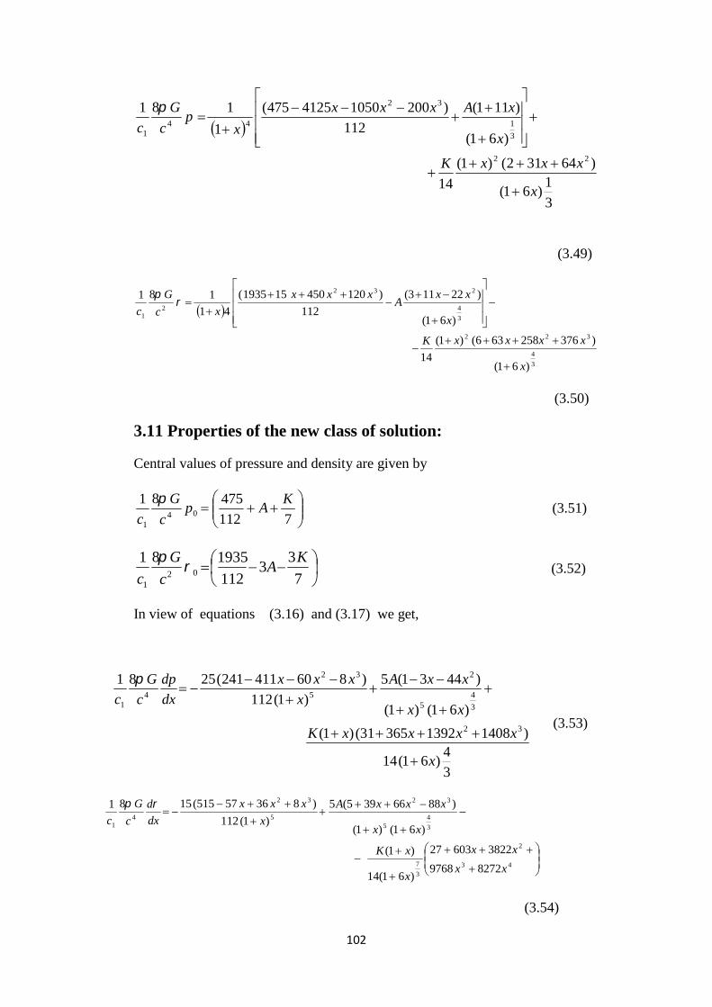
102
3
1)61(
)64312()1(
14
)61(
)111(
112
)20010504125475(
1
181
22
3
1
32
441
x
xxxK
x
xAxxx
xp
c
G
c
(3.49)
3
4
322
3
4
232
21
)61(
)376258636()1(
14
)61(
)22113(
112
)120450151935(
41
181
x
xxxxK
x
xxA
xxx
xc
G
c
(3.50)
3.11 Properties of the new class of solution:
Central values of pressure and density are given by
7112
4758104
1
KAp
c
G
c
(3.51)
7
33
112
19358102
1
KA
c
G
c
(3.52)
In view of equations (3.16) and (3.17) we get,
3
4)61(14
)1408139236531()1(
)61()1(
)4431(5
)1(112
)860411241(2581
32
3
45
2
5
32
41
x
xxxxK
xx
xxA
x
xxx
dx
dp
c
G
c
(3.53)
43
2
3
7
3
45
32
5
32
41
82729768
382260327
)61(14
)1(
)61()1(
)8866395(5
)1(112
)83657515(1581
xx
xx
x
xK
xx
xxxA
x
xxx
dx
d
c
G
c
(3.54)

103
AK
dx
dp
c
G
c5
112
6025
14
3181
0
41
(3.55)
AK
dx
d
c
G
c25
112
7725
14
2781
0
41
(3.56)
)(70)61)((16
30)()1(
)](70)61()(16
50)()1([
)61(1
3/76
3/46
2
xATxxHxMxK
xQAxxPxNxKx
d
dp
c
(3.57)
where
32 83657515)( xxxxH 432 82749768382260327)( xxxxxM
32 8866395)( xxxxT 32 1408139236531)( xxxxN
32 860411241)( xxxxP
24431)( xxxQ
AK
AK
d
dp
c750
8
772527
708
602531
1
02
(3.58)
3.12 Boundary Conditions:The solutions so obtained are to be matched over the boundary with Reissner-
Nordstrom metric:
22
222222
1
2
22 2
1)sin(2
1 dtr
e
r
GMddrdr
r
e
r
GMds
(3.59)
which requires the continuity of ee , and q across the boundary r = rb
The condition (3.41) can be utilized to compute the values of arbitrary constantsA as follows:
Pressure at p( r = rb) = 0 gives
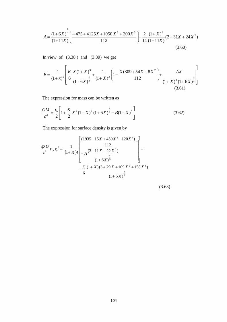
104
)24312()111(
)1(
14112
20010504125475
)111(
)61( 26323
1
XXX
XkXXX
X
XA
(3.60)
In view of (3.38 ) and (3.39) we get
3
13
2
3
3
1
3
5
)61()1(112
854309(1
)1(
1
)61(
)1(
6)1(
1
XX
AXXXX
XX
XXK
xB
(3.61)
The expression for mass can be written as
53
222
2)1()61()1(
21
2XBXXX
Kr
c
GM b (3.62)
The expression for surface density is given by
3
4
32
3
4
2
32
2
2
)61(
)158109293()1(
6
)61(
)22113(112
)120450151935(
41
18
X
XXXXK
X
XXA
XXX
Xr
c
Gbb
(3.63)

105
Table 3.6 : The variation of various physical parameters at the centre, surface density,electric field intensity on the boundary, mass and radius of stars with different
values of K and X = .1 .
K 041
81p
c
G
c
02
1
81
c
G
c 0
02
1
p
c 02)(
1xd
dp
c 0zbr
c
E
1
22
2
8bb r
c
G
M
Mbr in
km
2 3.5774 19.2676 0.1856 0.5603 0.31 0.150 1.177 0.4917.78
4 3.17103 20.4857 0.1548 0.4514 0.34 0.300 1.343 0.8417.45
6 2.7653 21.7039 0.12741 0.3757 0.38 0.451 1.091 1.1717.12
8 2.3593 22.922 0.1029 0.3199 0.42 0.601 1.048 1.5016.78
10 1.9538 24.1401 0.08091 0.2772 0.45 0.752 1.005 1.8016.43
12 1.5472 25.3582 0.0610 0.2434 0.50 0.902 0.962 2.1216.07
14 1.1412 26.5763 0.04294 0.2161 0.55 1.053 0.919 2.3715.71
16 0.7332 27.7944 0.02645 0.1934 0.60 1.203 0.876 2.6315.34
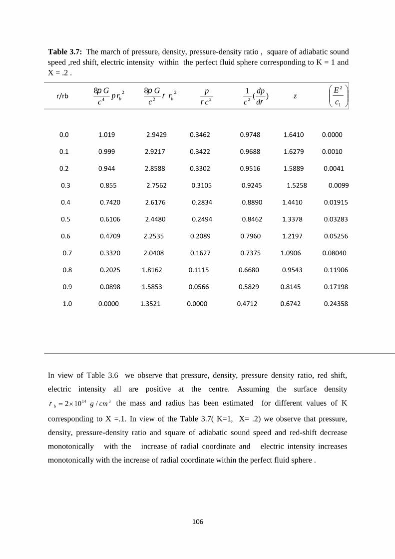
106
Table 3.7: The march of pressure, density, pressure-density ratio , square of adiabatic soundspeed ,red shift, electric intensity within the perfect fluid sphere corresponding to K = 1 andX = .2 .
K r/rb 2
4
8brp
c
G 2
2
8brc
G
2c
p
)(
12 d
dp
cz
1
2
c
E
0.0 1.019 2.9429 0.3462 0.9748 1.6410 0.0000
0.1 0.999 2.9217 0.3422 0.9688 1.6279 0.0010
0.2 0.944 2.8588 0.3302 0.9516 1.5889 0.0041
0.3 0.855 2.7562 0.3105 0.9245 1.5258 0.0099
0.4 0.7420 2.6176 0.2834 0.8890 1.4410 0.01915
0.5 0.6106 2.4480 0.2494 0.8462 1.3378 0.03283
0.6 0.4709 2.2535 0.2089 0.7960 1.2197 0.05256
0.7 0.3320 2.0408 0.1627 0.7375 1.0906 0.08040
0.8 0.2025 1.8162 0.1115 0.6680 0.9543 0.11906
0.9 0.0898 1.5853 0.0566 0.5829 0.8145 0.17198
1.0 0.0000 1.3521 0.0000 0.4712 0.6742 0.24358
In view of Table 3.6 we observe that pressure, density, pressure density ratio, red shift,
electric intensity all are positive at the centre. Assuming the surface density
314 /102 cmgb the mass and radius has been estimated for different values of K
corresponding to X =.1. In view of the Table 3.7( K=1, X= .2) we observe that pressure,
density, pressure-density ratio and square of adiabatic sound speed and red-shift decrease
monotonically with the increase of radial coordinate and electric intensity increases
monotonically with the increase of radial coordinate within the perfect fluid sphere .

107
Fig 3.2: The Behaviour of pressure, density, pressure-density ratio , square of
adiabatic sound speed, red shift Z, electric intensity1
2
c
Eversus radius for
K = 1, X = .2.
3.13: The solution for n = 3
Case IV- When n = 3
We have the expression for electric intensity as
3
23
1
2
)61()1(2
1xxxK
c
E
(3.64)
201
2 K
c
E
dx
d
x
(3.65)
The electric intensity is minimum at the centre and monotonically increasing for all values
K > 0. Also at the centre it is zero. Thus we have, 0,0 1 cK .
In view of equations (3.11), (3.12), (3.13) we get ,
0
0.5
1
1.5
2
2.5
3
3.5
0 0.2 0.4 0.6 0.8 1
fractional radius r/rb
pressure
density
pressure/density
d(pressure)/d(density)
electric field
red shift
108
3
3
1
2
33/1
5
)1(
)61(112
)854309(1
)1(
1
)61(
)1(
8
x
x
Axxxx
xx
xxKe
(3.66)
3
1)61(
)70322()1(
16)61(
)111(
112
)20010504125475(
1
181 23
3
1
32
441 x
xxxK
x
xAxxx
xp
c
G
c
(3.67)
3
4
323
3
4
232
21 )61(
)436298686()1(
16)61(
)22113(
112
)120450151935(
41
181
x
xxxxK
x
xxA
xxx
xc
G
c
(3.68)
3.14: Properties of the new class of solution (n = 3)
Central values of pressure and density are given by
8112
4758104
1
KAp
c
G
c
(3.69)
8
33
112
19358102
1
KA
c
G
c
(3.70)
In view of equations (3.16) and (3.17) we get,
34
)61(16
)1960175437034()1(
)61()1(
)4431(5
)1(112
)860411241(2581 322
3
45
2
5
32
41 x
xxxxK
xx
xxA
x
xxx
dx
dp
c
G
c
(3.71)

109
432
3
7
2
3
45
32
5
32
41
1220813532507879238
)61(16
)1(
)61()1(
)8866395(5
)1(112
)83657515(1581
xxxx
x
xK
xx
xxxA
x
xxx
dx
d
c
G
c
(3.72)
AK
dx
dp
c
G
c5
112
6025
16
3481
04
1
(3.73)
AK
dx
d
c
G
c25
112
7725
16
3881
04
1
(3.74)
In view of equation (3.18) we get
)(80)61)((14
30)()1(
)](80)61()(14
50)()1([)61(1
3/77
3/47
2
xATxxHxMxK
xQAxxPxNxKx
d
dp
c
(3.75)
where
32 83657515)( xxxxH 432 1220813532507879238)( xxxxxM
32 8866395)( xxxxT 32 860411241)( xxxxP
24431)( xxxQ
AK
AK
d
dp
c400
7
772538
807
602534
1
02
(3.76)
Pressure at )( brrp = 0 gives
110
)70322()111(
)1(
16112
20010504125475
)111(
)61( 27323
1
XXX
XKXXX
X
XA
(3.77)
In view of (3.38) and (3.39) we get
3
13
2
3
3
1
5
5
)61()1(112
854309(1
)1(
1
)61(
)1(
6)1(
1
XX
AXXXX
XX
XXK
xB
(3.78)
3
18
2
8
3
1
)61()1(112
854309(1
)1(
1
)61(6
XX
AXXXX
XX
XKB
(3.79)
The expression for mass can be written as
53
232
2)1()61()1(
21
2XBXXX
Kr
c
GM b (3.80)
The expression for surface density is given by
3
4
323
3
4
232
2
2
)61(
)436298686()1(
16
)61(
)22113(
112
)120450151935(
41
1
8
X
XXXXK
X
XXA
XXX
XXr
c
Gbb
(3.81)

111
Table 3.8: The variation of various physical parameters at the centre, surface density,
electric field intensity on the boundary, mass and radius of stars with different
values of K and X = .1
K K04
1
81p
c
G
c
02
1
81
c
G
c 0
02
1
p
c02
)(1
xd
dp
c 0z
brc
E
1
2
2
2
8bb r
c
G
M
Mbr in
in kmk
0.02 3.98 18.06 0.220 0.728 0.7536 0.0018 1.219 2.909 18. 10
0.08 3.96 18.09 0.219 0.721 0.7540 0.0072 1.218 2.912 18.09
0.2 3.94 18.16 0.217 0.709 0.7550 0.0182 1.215 2.919 18.06
0.4 3.90 18.28 0.213 0.689 0.7566 0.0364 1.210 2.930 18.03
0.6 3.86 18.40 0.209 0.670 0.7582 0.0546 1.206 2.941 17.99
0.8 3..82 18.52 0.206 0.652 0.7598 0.072 1.201 2.952 17.96
4.0 3.18 20.44 0.155 0.452 0.7862 0.364 1.125 3.118 17.38
8.0 2.38 22.83 0.104 0.320 0.8210 0.728 1.031 3.296 16.64
12.0 1.59 25.22 0. 063 0.243 0.8578 1.092 0.936 3.438 15.86
19.0 0.19 29.41 0.006 0.165 0.9280 1.729 0.771 3.59 14.39

112
Table 3.9: The values of various physical parameters at the center, surface density,electric field intensity on the boundary, mass and radius of star with different values of Xand K = 2
K X04
1
81p
c
G
c
02
1
81
c
G
c 0
02
1
p
c 02)(
1xd
dp
c 0z
brc
E
1
2
2
2
8bb r
c
G
M
Mbr in km
in k
0.001 0.10 28.67 0.003 0.389 0.007 0.001 0.029 0.009 2.81
0.004 0.31 29.06 0.010 0.395 0.029 0.004 0.113 0.071 5.53
0.01 0.68 27.93 0.024 0.406 0.074 0.017 0.264 0.256 8.42
0.02 1.23 26.30 0.046 0.424 0.149 0.022 0.470 0.624 11.23
0.04 2.08 23.74 0.087 0.459 0.299 0.051 0.765 1.360 14.33
0.06 2.72 21.83 0.124 0.495 0.451 0.087 0.959 2.003 16.05
0.08 3.20 20.37 0.157 0.528 0.607 0.130 1.088 2.549 17.09
0.1 3.58 19.24 0.186 0.561 0.769 0.182 1.172 3.017 17.75
0.2 4.38 16.83 0. 260 0.656 1.741 0.584 1.177 4.712 17.78
0.3 3.78 18.64 0.203 0.580 3.497 1.309 0.588 5.128 12.57
From the Table 3.9 we observe that central pressure, the ratio of pressure anddensity, surface density, radius increases with the increasing values of X upto X =.2 and then decreases corresponding to K = 2. Beyond the value of X= .3 the solution is not well behaved

113
Table 3.10 : The march of pressure, density, pressure-density ratio, square ofadiabatic sound speed , red shift, electric intensity within the perfect fluidsphere corresponding to K = 1 and X = .1
r/rb2
4
8brp
c
G 2
2
8brc
G
2c
p
)(
12 d
dp
cz
1
2
c
E
0.0 0.376 1.870 0.2013 0.6331 0.761 0 .0000
0.1 0.371 1.861 0.1994 0.6319 0.757 0.0005
0.2 0.355 1.835 0.1934 0.6281 0.744 0.0020
0.3 0.329 1.794 0.1834 0.6216 0.722 0.0047
0.4 0.294 1.734 0.1693 0.6120 0.692 0.0089
0.5 0.252 1.668 0.1512 0.5990 0.656 0.0147
0.6 0.205 1.588 0.1290 0.5821 0.612 0.0228
0.7 0.154 1.498 0.1028 0.5606 0.562 0.0335
0.8 0.101 1.402 0.0724 0.5340 0.508 0.0478
0.9 0.049 1.301 0.0380 0.5014 0.449 0.0666
1.0 0.000 1.196 0.0000 0.4620 0.388 0.0910
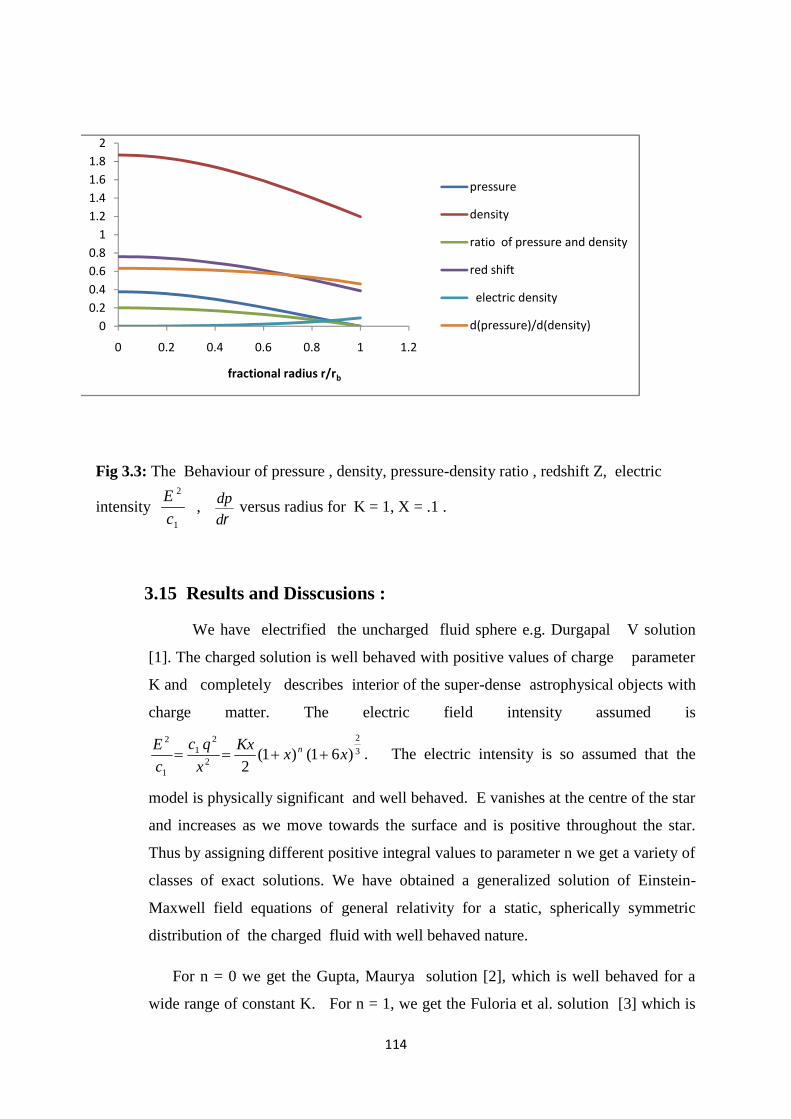
114
Fig 3.3: The Behaviour of pressure , density, pressure-density ratio , redshift Z, electric
intensity1
2
c
E,
d
dp versus radius for K = 1, X = .1 .
3.15 Results and Disscusions :
We have electrified the uncharged fluid sphere e.g. Durgapal V solution
[1]. The charged solution is well behaved with positive values of charge parameter
K and completely describes interior of the super-dense astrophysical objects with
charge matter. The electric field intensity assumed is
3
2
2
21
1
2
)61()1(2
xxKx
x
qc
c
E n . The electric intensity is so assumed that the
model is physically significant and well behaved. E vanishes at the centre of the star
and increases as we move towards the surface and is positive throughout the star.
Thus by assigning different positive integral values to parameter n we get a variety of
classes of exact solutions. We have obtained a generalized solution of Einstein-
Maxwell field equations of general relativity for a static, spherically symmetric
distribution of the charged fluid with well behaved nature.
For n = 0 we get the Gupta, Maurya solution [2], which is well behaved for a
wide range of constant K. For n = 1, we get the Fuloria et al. solution [3] which is
00.20.40.60.8
11.21.41.61.8
2
0 0.2 0.4 0.6 0.8 1 1.2
fractional radius r/rb
pressure
density
ratio of pressure and density
red shift
electric density
d(pressure)/d(density)

115
also well behaved for a wide range of constant K, hence suitable for modeling of
super dense star.
In view of Table 3.1 we observe that all the physical parameters (p, , ,2c
p
Eandzd
dp,
) are positive at the centre and within the limit of realistic equation
of state and well behaved conditions for all values of K satisfying the inequality
100 K corresponding to X = .2 . However, for any value of K > 10,
corresponding to X= .2 surface density is negative. Table 3.2 shows the values of
different physical parameters for different values of K corresponding to X = .1 .
From Table 3.2 we observe that the solution is well behaved for the values of K up
to 20 corresponding to X = .1. Beyond this value of K the solution is not well
behaved. The mass and red shift increases with the increasing values of K but the
radius decreases with K. Table 3.3 shows the values of different parameters for
different values of K corresponding to X = .01. From Table 3.4 we observe that the
solution is well behaved for the values of K up to 44 . Hence we may conclude that
for the solution (n =1), as the value of X is decreased the solution becomes well
behaved for larger values of K. The solution for n = 2 is also well behaved for all
the values of K satisfying the inequality 160 K corresponding to X = .2.
Similarly the solution for n = 3 is well behaved for the values of K satisfying the
inequality 19K corresponding to X=.1 .
3.15 a. Modeling of superdense star for the solution n = 1
We present here a model of super dense star based on the particular solution
(n = 1)discussed above corresponding to K = 0.35 with 2.X ,by assuming surface
density;314 /102 cmgb .The resulting well behaved model has the heaviest star
occupying a mass 5.523 MΘ with its radius 13.98 km. Corresponding to K = 1 and
X = .1 ,the maximum mass of the star comes out to be 2.95 MΘ with linear dimension
17.95 km.Corresponding to K = 20 and X = .1 the maximum mass of the star comes
out to be 3.55 MΘ with linear dimension 14.92 km. Corresponding to K = 44 and X =

116
.01 the maximum mass of the star comes out to be 0.2660 MΘ and radius 8.345 km.
Thus we get the mass of the stellar object with in the range of neutron star and white
Dwarf. From Tables 3.1, 3.2, 3.3 it is clear that as the value of X is decreased the
solution becomes well behaved for larger values of K. In absence of the charge we
are left behind with the regular and well behaved fifth model of Durgapal [1].
3.15 b. Modeling of superdense star for n = 2 :
Table 3.6 shows the variation of different physical parameters for different
values of K corresponding to X = .1. The solution is well behaved for the value of K
up to 16. For the solution n = 2 the mass of a star is maximized with all degrees of
suitability and by assuming the surface density 314 /102 cmgb . Corresponding
to K = 16 and X = .1 the maximum mass of the star comes about to be 2.63 MΘ with
linear dimension 15.34 km. Corresponding to K = 6 and X = .1 the maximum mass
of the star comes about to be 1.17 MΘ with linear dimension 17.12 km. Table 3.7
shows that pressure, density, pressure-density ratio , red shift decrease as we move
from centre to the surface of superdense star. However the electric intensity increases
as the surface of the star approaches. Thus for the solution corresponding to n = 2 we
may construct the models for super massive objects. we arrive at the conclusion that
under well behaved conditions this class of solutions gives us the mass of super
dense object within the range of neutron star and quark star.
3.15 c. Modeling of super dense star for n = 3.
Table 3.8 shows the values of different physical quantities for different values of K
corresponding to X = .1. The solution is well behaved for the values of .001< K < 19.
As the value of K increases the mass and red shift increase but radius decreases.For the
solution n = 3 the mass of a star is maximized with all degrees of suitability and by
assuming the surface density 314 /102 cmgb . Corresponding to K = 0.02 and X = .1
the maximum mass of the star comes about to be 2.0909 MΘ with linear dimension
18.10 km. Corresponding to K = 19 and X = .1 the maximum mass of the star comes about
to be 3.59 MΘ with linear dimension 14.39 km. Table 3.9 also shows the values
117
of different physical quantities for different values of X corresponding to K = 2.
Corresponding to K = 2 and X = 0.08 the maximum mass of the neutron star comes out to
be 2.549 MΘ with linear dimension 17.09 km. Corresponding to K = 2 and X = 0.1 the
maximum mass of the star comes out to be 3.017 MΘ with linear dimension 17.75 km.
We observe that with the increase of the value of n, although the solutions
become more complicated in terms of expressions, but they show the well behaved
nature and satisfy all the necessary conditions to be physically realizable. For n = 1, n
= 2 and n = 3 we have obtained new solutions of Einstein- Maxwell field equations
, which have been studied extensively exposing their well behaved nature.The solutions
for n = 4, n = 5, n = 6 and so on can be also studied likewise. In the absence of the
charge we are left behind with the regular and well behaved fifth model of Durgapal [1].

118
3.16 References:
[1] Durgapal, M.C. : . “A class of new exact solutions in general
relativity” , Journal of Phy. A Math Gen, 15 , 2637 ( 1982).
[2] Gupta,Y.K., Maurya S.K., : “A class of regular and well behaved
relativistic super dense star models” , Astrophys. Space Sci.,
334(1),155 (2011) .
[3] Fuloria, P., Tiwari, B.C., Joshi, B. C., : “Well behaved class of
charge Analogue of Durgapal’s relativistic exact solution”, Journal Of
Modern Physics, 2,1156 (2011).
[4] R. Stettner, “On the stability of homogeneous, spherically symmetric,
charged fluids in relativity”, Ann. Phys. (NY) 80 212 (1973).
[5] P. G. Whitman, R.C. Burch: “Charged spheres in general relativity”,
Phys. Rev. D 24 (1981) 2049.
[6] de Felice F., Y. Yu and J. Fang J., Mon. Not. R. Astron. Soc. 277, L17
(1995).
[7] Bayin, S. S.: “Solutions of Einstein's field equations for static fluid
spheres” , Phys. Rev. D18, 2745 (1978).
[8] Ray, S. et al.: “Dark Energy Models with a Time-Dependent
Gravitational Constant”, Int. J. Mod. Phys. D16, 1745, (2007).
[9] Bonnor, W. B.: “The equilibrium of a charged sphere”, Mon. Not. R.
Astron. Soc. 129, 443 (1965).
[10] Herrera, L. and Santos, N. O.: “Local anisotropy in self-gravitating
systems”, Phys. Rep. 286 53(1997).

119
[11] Bondi, H. : “Gravitational Bounce in General Relativity”, Mon. Not.
R. Astr. Soc. 142 333 (1969).
[12] Tikekar, R.: “Spherical charged fluid distributions in general
relativity”, J. Math. Phys. 25, 1481(1984).
[13] Humi, M. and Mansour, J.: “Interior solutions to Einstein-Maxwell
equations in spherical and plane symmetry when p=nρ”, Phys. Rev. D,
29 1076 (1984).
[14] Bonnor, W. B. and Wickramasuriya, S .B. P.: “Are very large
gravitational redshifts possible”, Mon. Not. R. Astr. Soc. 170, 643
(1975).
[15] Ivanov, B. V. “Static charged perfect fluid spheres in
general relativity” , Phys. Rev. D, 65 104001(2002).
[16] Ray, S., et al. : “Electrically charged compact stars and formation of
charged black holes”, Phys. Rev. D 68, id. 084004(2003).
[17] Bekenstein, J.: Phys. Rev 4 2185(1975).
[18] Graves, J. C. and Brill, D.R. : “Oscillatory Character of Reissner
Nordstorm Metric for an Ideal Charged Worm-hole”, Physical
Review, 120(4),1507(1960).
[19] Ray, S., Das, B.: “Tolman-Bayin type static charged fluid spheres in
general relativity” , Mon. Not. R. Astron. Soc. 349, 1331(2004).
[20] Bonner, W.B., Cooperstock, F.I.: “Does the electron contain negative
mass?”, Phys. Lett. A 139, 442(1989).
[21] Bonnor, W. B, “The mass of a static charged sphere”, Z. Phys. 160,
59 (1960).
120
[22] Efinger, H. J.: Z. Phys. 188 31(1965).
[23] Kyle, C. F., Martin, A. W.: “Self-energy considerations in general
relativity and the exact fields of charge and mass distributions”,
Nuovo Cimento 50, 583 (1967).
[24] Krori, K. D., Barua, J.: “A singularity-free solution for a charged fluid
sphere in general relativity”, J. Phys. A Mathematical and general 8,
508(1975).
[25] Nduka, A.: “Charged fluid sphere in general relativity”, Gen. Relativ.
Gravitation 7, 493 (1976).
[26] Durgapal, M.C., Fuloria, R.S.: “Analytic stellar model for super-dense
star”, Gen. Relativ. Gravit. 17, 671(1985).
[27] Gupta, Y.K., Maurya, S. K.: “A class of charged analogues of
Durgapal and Fuloria superdense star”, Astrophys. Space Sci.
331(1),135 (2010).
[28] Schwarzschild, K.: “On the Gravitational Field of a Mass Point
According to Einstein's Theory”, Sitzer. Preuss. Akad. Wiss. Berlin ,
424,189 (1916).
[29] Bijalwan, Naveen, Gupta, Y. K.: “Nonsingular charged analogues of
Schwarzschild's interior solution”, Astrophysics and Space Science,
317,251(2008).
[30] Gupta,Y. K., Kumar, M. : “A superdense star model as charged
analogue of Schwarzschild's interior solution”, General Relativity and
Gravitation 37(3), 575 (2005).
121
[31] Kuchowich, B.: “General Relativistic fluid spheres. I. New solutions
for spherically symmetric matter distribution”, Acta Phys. Pol.33 ,
541(1968b).
[32] Nduka, A.: “Some exact solutions of charged general relativistic fluid
spheres”, Acta Phys. Pol. B8, 75 (1977).
[33] Tolman, R. C.: “Static solutions of Einstein’s field equations for
spheres of Fluid ”, Phys. Rev. 55, 367 (1939).
[34] Cataldo, M., Mitskievic, N. V. : “Static charged fluid surrounded by a
black antihole: an enlarged Klein solutio”, Class. Quantum Gravity
9,545 (1992).
[35] Heintzmann, H.: “New exact static solutions of Einstein field
equations”, Z. Phys. 228, 489 (1969).
[36] Pant, N. et al.: “Well behaved class of charge analogue of
Heintzmann’s relativistic exact solution”, Astrophys. Space Sci.,
332(2), 473 (2011a).
[37] Pant, N. , Tewari, B. C., Fuloria, P.: “Well Behaved Parametric Class of
Exact Solutions of Einstein-Maxwell Field Equations in General
Relativity”, Journal of Modern Physics, 2 (12) 1538 ( 2011).
[38] Pant, M. J. and Tewari, B. C., “Well Behaved Class of Charge Analogue
of Adler’s Relativistic Exact Solution” , Journal of Modern Physics, 2 (
6) 481( 2011).
[39] Pant, N., Mehta, R. N., (Joshi) Pant, M.: “Well behaved class of charge
analogue of Heintzmann’s relativistic exact solution”, Astrophys. Space
Sci. 332(2), 473(2011).

122
[40] Florides, P. S.: “The complete field of charged perfect fluid spheres and
of other static spherically symmetric charged distributions”, J. Phys. A,
Math. Gen. 16, 1419 (1983).
[41] Adler, R.: “A fluid sphere in general relativity”, J. Math. Phys. 15, 727
(1974).
[42] Singh, T., Yadav, R. B. S.: “Some exact solutions of charged fluid
spheres in General relativity”, Acta Phys. Pol. B 9, 475 (1978).
[43] Delgaty, M.S.R., Lake, K.: “Physical Acceptability of Isolated, Static,
Spherically Symmetric, Perfect Fluid Solutions of Einstein’s
Equations”, Comput. Phys. Commun. 115, 395 (1998) .
[44] Pant, N. et al. : “New class of regular and well behaved exact solutions in
general relativity”, Astrophys. Space Sci. 330(2) 353 (2010).
[45] Leibovitz, C.: “Spherically symmetric static solutions of Einstein’s field
equations”, Phys. Rev. D 185, 1664 (1969).
[46] Pant, N.: “Some new exact solutions with finite central parameters and
uniform radial motion of sound ”, Astroph. Space Sci. 331, 633 (2011).
[47] Dionysiou, D.D. :“Equilibrium of a Static Charged Perfect Fluid
Sphere”,Astrophys. Space Sci. 85(1-2), 331 (1982).

Chapter IVRadiating fluid ball models with
horizon free gravitational collapse
123
Chapter IV
Radiating fluid ball models withhorizon free gravitational collapse5
In this chapter we have revisited a solution of the radiating fluid ball problem
proposed by Tewari[1], (hereafter referred to as the BCT solution II ) in which the
horizon is never encountered. By assuming the life time of quasars 107 years we
have constructed different approximate models of quasars for different
combinations of the constants X , Y and Z appearing in the solution. The interesting
feature of all the models is that the rate of decrease of mass is balanced by the rate
of contraction of the boundary and the collapsing process continuous without the
reach of horizon of the black hole. There is an only singularity i.e. the naked
singularity. We have also studied the variation of pressure, density, pressure density
ratio and luminosity within the radiating fluid ball with the increase of r at any
particular time. At any particular point within the sphere the pressure and density
increases with time and attains the infinite value as t tends to 107 years. The
expressions for mass and radius of the collapsing ball are linear functions of time.
5A part of this chapter has been communicated for publication.

124
4.1 Introduction:
One of the most important and outstanding problem of gravitational collapse
is whether it ends in a black hole or a naked singularity. According to general theory of
relativity the collapsing massive star must terminate into a space-time singularity, where the
matter energy densities , space-time curvature and other physical quantities blow up. It then
becomes important to know whether such ultra dense regions , formed during stellar collapse
will be visible to an external observer in the universe, or whether they will be always hidden
within an event horizon of gravity that could form as the star collapses. This is one of the
most important issue in the physics of gravitational collapse today. According to cosmic
censorship hypothesis the space time singularity forming in collapse always hides within the
event horizon , never to be seen by external observers. Or there is no possibility of the
existence of naked singularity. However, many models of radiating fluid spheres have been
discovered which admit the existence of naked singularity . The collapse of radiating fluid
spheres may be studied to ascertain the final outcome of the collapse. We know that
gravitational collapse is a highly dissipating energy process which plays important role in
the structure formation in the universe. The dissipation of energy from collapsing fluid
distribution is described in two limiting cases. The first case , the free streaming
approximation is modeled by means of an outflowing null fluid and the second case ,the
diffusion approximation is modeled by heat flow type vector. Various scenarios of
gravitational collapse have been considered within the realm of relativistic astrophysics both
in the free streaming approximation and in the diffusion approximation .There exist a
number of solutions in free streaming limiting case in which the horizon is never
encountered. These solutions may be useful for constructing the approximate models of
quasar in which the radiation emitted by the collapsing object is significant.
We also know that during some stages of evolution star may radiate away a
large chunk of energy in the form of photons or neutrinos or both. In a normal star the
stellar radiation is a very slow process and does not have any significant effect in the
interior and exterior gravitational field of a star. However there are some high energy
astrophysical events such as Quasars and Supernova burst, where this radiation process
is strong and cannot be ignored . So to make the real assessment of such events the
general relativistic field equations must be studied taking into account the out flowing
125
radiation. Our aim is also to investigate the solution of Einstein field equations for the
radiating fluid ball problem in which the horizon is never encountered. Vaidya initiated the
problem of solving the field equations of general relativity for physically realizable radiating
fluid distributions. Solutions for the radiating fluid structures corresponding to isotropic
coordinate form, general metric form, and conformally metric form have been obtained [1-3]
by solving the modified field equations proposed by Misner[4], Lindquist et al.[5] for an
adiabatic distribution of matter. Bayin [6] has also obtained some solutions of Einstein’s
field equations for radiating fluid distribution. Herrera et al.[7] have constructed the radiating
fluid models from known static solutions of Einstein’s field equations. On the similar
grounds a number of models have been proposed by De’Oliveira et al. [8-10], Bonnor et al.
[11], Kramer [12], Maharaj et al. [13-14] and others. A number of studies have been
proposed by Herrera et al. [15-20], Herrera and Santos [21], Mitra [22], Naidu and Govinder
[23] and references there in for the radiating fluid ball models. All these studies describe a
collapsing fluid dissipating energy.
Realistic models of radiating fluid spheres in general relativity are few on
account of associated mathematical complexities. Vaidya, P. C. [24-25] solved the field
equations of general relativity for physical meaningful models of radiating fluid spheres.
The interior space-time metric is matched with Vaidya exterior space-time metric [26] at
zero pressure boundary. Baneerji et al.[27] and Pant and Tewari[28] have proposed the
radiating stellar models in which the horizon is never encountered. We have revisited the
solution of radiating fluid ball problem proposed by Tewari[1]. We have shown that the
collapse of radiating fluid ball will result into the formation of naked singularity i.e.
horizon will never form.
We have also constructed the approximate models of Quasar by considering
the BCT solution II in detail. To investigate the final outcome of collapse we
have worked out the mass-radius gradient for all the proposed models of Quasars.
If 1)(/)(20 2 uRcuMG s the model will be horizon free favouring the
existence of naked singularity.
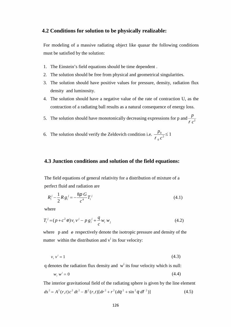
126
4.2 Conditions for solution to be physically realizable:
For modeling of a massive radiating object like quasar the following conditions
must be satisfied by the solution:
1. The Einstein’s field equations should be time dependent .
2. The solution should be free from physical and geometrical singularities.
3. The solution should have positive values for pressure, density, radiation flux
density and luminosity.
4. The solution should have a negative value of the rate of contraction U, as the
contraction of a radiating ball results as a natural consequence of energy loss.
5. The solution should have monotonically decreasing expressions for p and2c
p
6. The solution should verify the Zeldovich condition i.e. 12
0
0 c
p
4.3 Junction conditions and solution of the field equations:
The field equations of general relativity for a distribution of mixture of a
perfect fluid and radiation are
ji
ji
ji T
c
GgRR
4
8
2
1 (4.1)
where
jij
ij
ij
i wwc
qgpvvcpT )( 2 (4.2)
where p and respectively denote the isotropic pressure and density of the
matter within the distribution and vi its four velocity:
1ii vv (4.3)
q denotes the radiation flux density and wi its four velocity which is null:
0ii ww (4.4)
The interior gravitational field of the radiating sphere is given by the line element
)]sin([),(),( 2222222222 ddrdrtrBdtctrAds (4.5)

127
We choose r as a co moving coordinate so that ).0,0,0,( 1 Av i
We choose iw such that [4]
,1 11
rB
tcA
xw
ii
(4.6)
which implies that q is the energy density of the radiation in the rest frame of the
fluid [4,5].
jiji wwqvvq (4.7)
From Equation (4.1) we obtain four independent equations, which in view of Eq.
(4.2) can be written as
22Tp (4.8)
,22
00
11
2 TTTc (4.9)
,)( 01
213
TwB
A
c
q (4.10)
01
22
11 T
B
ATT (4.11)
The luminosity or neutrino flux is given by
qBrL 224 (4.12)
The space time external to a radiating fluid ball of mass M(u) is filled with pure
radiation , for which a suitable metric is Vaidya’s radiating metric (Vaidya,
1953)[24]
)sin(22
1 222222
2 ddRdRduduRc
GMds
(4.13)
where R is the radial coordinate. The condition describing the junction of (4.5) and
(4.13) over the hyper surface r = rs or equivalently )(uRR s are ( Misner,1965)[4]
),,()( trBruR sss (4.14)
,1),(s
s B
Br
A
BrdudtctrA
(4.15)
,0),( trp s (4.16)

128
s
s B
Brr
A
BBr
G
ctrmuM
232
2
232 )(2
2),()(
(4.17)
The expression for L is given by
2
3 1s
B
Br
A
BrL
du
dMcL
(4.18)
A prime and a dot here after denote differentiation with respect to r and ct, respectively
In order to solve the field equations Tewari [1]used the following method,
Tewari wrote
),()(),( tlrftrA (4.19)
),()(),( tnrhtrB (4.20)
The equation (4.11) transform into
022
22
2
f
fh
k
n
rf
f
f
f
hr
h
hf
hf
h
h
h
h (4.21)
Tewari assumed that
lsn2
1 (4.22)
where s is an arbitrary constant. Equation (4.21) then reduces to the r-dependent
equation
02
22
2
f
fhs
rf
f
f
f
hr
h
hf
hf
h
h
h
h(4.23)
This is an ordinary differential equation in two unknown functions h and f.
Tewari assumed that
02
2
2
fr
f
f
f
f
f(4.24)
The solution obtained by Tewari [1] is
)/( 22 rXWf (4.25)
1
75234322222
7
2
5
4
3
2)()(
rrXrXsrXYZrXWh (4.26)
t is assumed as the proper time of the observer on the hyper surface r = rs,
This requires that
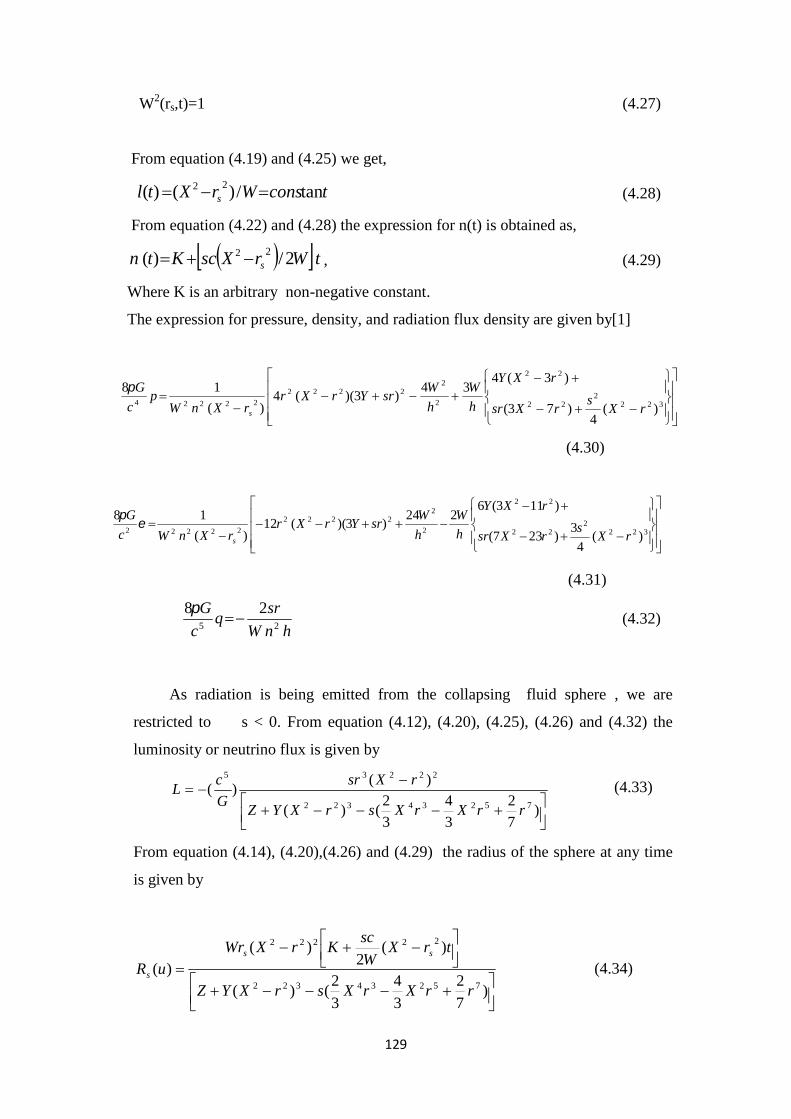
129
W2(rs,t)=1 (4.27)
From equation (4.19) and (4.25) we get,
tconsWrXtl s tan/)()( 22 (4.28)
From equation (4.22) and (4.28) the expression for n(t) is obtained as,
tWrXscKtn s 2/)( 22 , (4.29)
Where K is an arbitrary non-negative constant.
The expression for pressure, density, and radiation flux density are given by[1]
3222
22
22
2
22222
22224)(
4)73(
)3(434
)3)((4)(
18
rXs
rXsr
rXY
h
W
h
WsrYrXr
rXnWp
c
G
s
(4.30)
3222
22
22
2
22222
22222 )(4
3)237(
)113(6224
)3)((12)(
18
rXs
rXsr
rXY
h
W
h
WsrYrXr
rXnWc
G
s
(4.31)
hnW
srq
c
G25
28
(4.32)
As radiation is being emitted from the collapsing fluid sphere , we are
restricted to s < 0. From equation (4.12), (4.20), (4.25), (4.26) and (4.32) the
luminosity or neutrino flux is given by
)7
2
3
4
3
2()(
)()(
75234322
22235
rrXrXsrXYZ
rXsr
G
cL (4.33)
From equation (4.14), (4.20),(4.26) and (4.29) the radius of the sphere at any time
is given by
)
7
2
3
4
3
2()(
)(2
)()(
75234322
22222
rrXrXsrXYZ
trXW
scKrXWr
uRss
s (4.34)

130
The total energy inside the surface is given by [1]
375234322
275234322
2275234322
22322222224
622
2232
)7
2
3
4
3
2()(
)7
2
3
4
3
2()(
38)}7
2
3
4
3
2()({26
)5()(226)(4
22)(
rrXrXsrXYZ
rrXrXsrXYZ
rXrrXrXsrXYZsrY
rXrXsrYrrXs
rX
trXW
scKr
G
cWuM
ss
ssssss
ss
(4.35)
From Eq.(4.34) and (4.35) we observe that radius and mass are linear functions of
time .
The luminosity observed on the surface is given by
)7
2
3
4
3
2()(
)()(
75234322
22235
ssss
ss
rrXrXsrXYZ
rXsr
G
cL (4.36)
With the aid of equations (4.12), (4.16), (4.17), (4.25), (4.26) and (4.27) the
following equation is obtained .
2
75234322
232222
22
2
)7
2
3
4
3
2()(2
312)(
)(
41
ssss
ssss
s
s
rrXrXsrXYZ
rsXsrCrrX
rX
rdudtc
(4.37)
The total luminosity for an observer at rest at infinity is given by
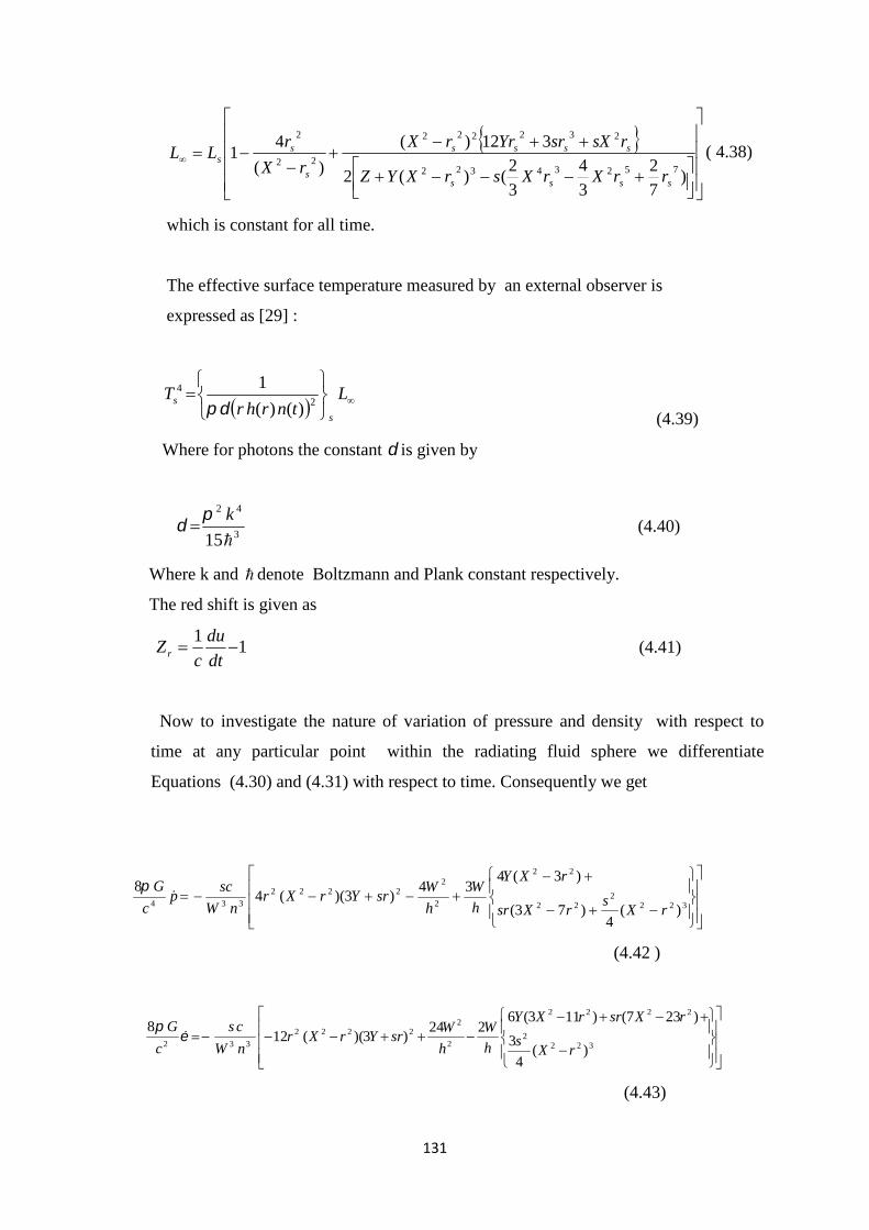
131
)7
2
3
4
3
2()(2
312)(
)(
41
75234322
232222
22
2
ssss
ssss
s
ss
rrXrXsrXYZ
rsXsrYrrX
rX
rLL ( 4.38)
which is constant for all time.
The effective surface temperature measured by an external observer is
expressed as [29] :
L
tnrhrT
s
s 24
)()(
1
(4.39)
Where for photons the constant is given by
3
42
15
k (4.40)
Where k and denote Boltzmann and Plank constant respectively.
The red shift is given as
11
dt
du
cZ r (4.41)
Now to investigate the nature of variation of pressure and density with respect to
time at any particular point within the radiating fluid sphere we differentiate
Equations (4.30) and (4.31) with respect to time. Consequently we get
3222
22
22
2
22222
334)(
4)73(
)3(434
)3)((48
rXs
rXsr
rXY
h
W
h
WsrYrXr
nW
scp
c
G
(4.42 )
3222
2222
2
22222
332 )(4
3
)237()113(6224
)3)((128
rXs
rXsrrXY
h
W
h
WsrYrXr
nW
cs
c
G
(4.43)

132
Where dot represents the differentiation with respect to time.
From Equations (4.42) and (4.43) it is clear that pressure and density increase with the
passage of time . On the other hand we can say that collapsing radiating fluid sphere
will approach towards space -time singularity, that will be visible by an external
observer .
To investigate the trend of variation of surface temperature with time, we may write
equation (4.39) as follows
4
1
2
14
1
)()()(
1
L
tnrhr
T
s
s
(4.44)
Differentiating Equation (4.44) with repect to time we get
4
1
2
3
2
14
1
22
)()(
)(
4
1
L
nrhr
rXcs
WT
s
ss
(4.45)
From Equation (4.45) we observe that surface temperature will also increase as time
evolves towards the infinity.
4.4. Different cases of BCT solution II for Quasar Model:
4.4.1 Case I
When X = 1, Y = 1, Z = 2, s = -2×10⁻¹⁰
And 2541.0sr
We have calculated the various parameters: like mass, radius, luminosity etc.
at any instant of time for the radiating fluid sphere. An approximate model of Quasar have
been constructed for the above mentioned values of constants. Equations (4.31) and (4.32)
give the march of p, ρ,2c
p
at any time t within the radiating fluid ball and
Eq.(4.33) gives the march of luminosity. We observe that pressure, density, luminosity
are positive within the radiating fluid sphere and3
12
c
p
everywhere within the ball.
Pressure and pressure-density ratio are monotonically decreasing however, luminosity

133
sis monotonically increasing with the increase of r. This combination of constants pertaining
to case I may be used for constructing the radiating fluid ball models . An approximate model
for Quasar has been constructed for the above said combination of constants.
Table 4.1:
The march of pressure , density, pressure-density ratio and Luminosity at anyinstant of time within the sphere (0 ≤ r ≤ rs).
(p in dynes cm-2, ε in g cm-3, and L in ergs s-1)
r/ rs pnWc
G)(
8 224
)(8 22
2nW
c
G2c
p
L
0.0 13.5000 108.0000 0.125 0
0.1 13.3821 108.3957 0.123 3.98×1044
0.2 13.0268 109.5898 0.118 3.18×1045
0.3 12.4288 111.6030 0.111 1.07×1046
0.4 11.5775 114.4712 0.101 2.52×1046
0.5 10.4600 118.2460 0.088 4.90×1046
0.6 9.05779 122.9974 0.073 8.40×1046
0.7 7.34590 128.8158 0.057 1.32×1047
0.8 5.29352 135.8162 0.038 1.95×1047
0.9 2.86151 144.1430 0.019 2.75×1047
1.0 0.0000 153.9762 0.000 3.71×1047

134
Fig 4.1: The variation of pressure with radius for the case I.
Fig 4 .2: The variation ofp
with radius for the case I.
02468
10121416
0 0.2 0.4 0.6 0.8 1 1.2
r/ rs
pressure
00.020.040.060.08
0.10.120.14
0 0.5 1 1.5
r/ rs
ratio of pressure anddensity

135
Fig 4.3: The variation of Luminosity from centre to surface.
Model of Quasar for case I:
In view of Equation (4.29 ) , we have
tWKtn 1806.2)( (4.46)
Consequently Equations (4.34), (4.35), (4.37 ) give us
tWKuRs 806.20788.0)( (4.47)
tWKuM 806.210525.1)( 26 (4.48)
dtcdu 1847.1 (4.49)
In view of Equations (4.41) and (4.49) the gravitational red shift Zr = .1847
For a life time of 107 years ,
our model has an initial mass of 6.65 × 10⁷ MΘ
and an initial linear dimension 6.8 × 1013 cm.
Our model is radiating energy at a constant rate i.e. L∞ = 3.359 × 1047 ergs/ sec.
0
5E+46
1E+47
1.5E+47
2E+47
2.5E+47
0 0.2 0.4 0.6 0.8 1
r/ rs
Luminosity inergs/second

136
4.4.2 Case II:
X= 1, Y= 1, Z= 3, s = -2×10⁻¹⁰
rs = 0.29741
we have studied the march of pressure, density, pressure-density ratio and
luminosity with in the radiating fluid sphere for case II. We have calculated the various
parameters: like mass, radius, luminosity, etc. at any instant of time and have
constructed an approximate model of Quasar. Equations (4.30) and (4.31) give
the march of p, ρ,2c
p
at any time t within the radiating fluid ball and in view of
Eq.(4.33) we get the march of luminosity .We observe that pressure, density,
luminosity are positive within the radiating fluid sphere and3
12
c
p
everywhere
with in the ball. Pressure and pressure-density ratio are monotonically decreasing ,
however , luminosity is monotonically increasing with the increase of r. We have
also found out an important parameter)(
)(22 uRc
uGM
s
that will tell us about
the nature of the gravitational collapse.

137
Table 4.2:
The march of p, ε, p/εc2, and L at any instant of time within the sphere (0 ≤ r ≤ rs)
(p in dynes cm-2, ε in g cm-3, and L in ergs s-1)
r/rs pnWc
G)(
8 224
)(
8 222
nWc
G2c
p
L
0.0 44.44 240.00 0.1857 0
0.1 44.036 241.06 0.1828 4.79×1044
0.2 42.807 244.28 0.1758 3.82×1045
0.3 40.747 249.73 0.1644 1.28×1046
0.4 37.836 257.55 0.1490 3.01×1046
0.5 34.046 267.95 0.2993 5.82×1046
0.6 29.337 281.20 0.1077 9.93×1046
0.7 23.657 297.67 0.0830 1.55×1047
0.8 16.938 317.86 0.0564 2.27×1047
0.9 9.0915 342.39 0.0286 3.17×1047
1.0 0.0000 372.07 0.0000 4.24×1047
________________________________________________________________________________

138
Fig 4.4: The variation of pressure from centre to surface .
Fig 4.5 : The variation of pressure-density ratio from centre to surface.
From Table 4.2 we observe that pressure, density, luminosity are positive and
p/εc2 < 1, everywhere with in the radiating fluid sphere. Pressure and pressure-
density ratio are monotonically decreasing, however, luminosity is monotonically
increasing with the increase of r.
In view of equation (4.29) ,we have
05
101520253035404550
0 0.2 0.4 0.6 0.8 1 1.2
Pressure
r/ rs
00.020.040.060.08
0.10.120.140.160.18
0.2
0 0.2 0.4 0.6 0.8 1 1.2
fractional radius r/ rs

139
tWKtn 1734.2)( (4.50)
Consequently we have
tWKuRs 734.206577.0)( (4.51)
tWKuM 734.210075.2)( 26 (4.52)
dtcdu 370.1 (4.53)
Assuming the life time of quasar 107 years ,
Our model has an initial mass of 8.82 ×10⁷ MΘ and
An initial linear dimension 5.51 ×1013 cm.
In view of equations (4.41) and (4.53) we get the gravitational red shift as .370.
Our model is radiating energy at a constant rate i.e. L∞= 2.902 × 1047 ergs /sec.
4.4.3. Case III
X = 1, Y = 1, Z = 4, s = -2×10⁻¹⁰
In view of Eq. (4.16) we get
rs = 0.317143
We have studied the march of pressure, density, pressure-density ratio and
luminosity with in the radiating fluid sphere. For the model to be realistic the pressure
, pressure-density ratio should be monotonically decreasing as we go from centre to
surface.
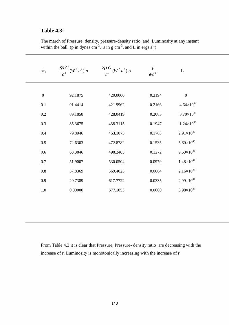
140
Table 4.3:
The march of Pressure, density, pressure-density ratio and Luminosity at any instantwithin the ball (p in dynes cm-2, ε in g cm-3, and L in ergs s-1)
r/rs pnWc
G)(
8 224
)(
8 224
nWc
G2c
p
L
0 92.1875 420.0000 0.2194 0
0.1 91.4414 421.9962 0.2166 4.64×1044
0.2 89.1858 428.0419 0.2083 3.70×1045
0.3 85.3675 438.3115 0.1947 1.24×1046
0.4 79.8946 453.1075 0.1763 2.91×1046
0.5 72.6303 472.8782 0.1535 5.60×1046
0.6 63.3846 498.2465 0.1272 9.53×1046
0.7 51.9007 530.0504 0.0979 1.48×1047
0.8 37.8369 569.4025 0.0664 2.16×1047
0.9 20.7389 617.7722 0.0335 2.99×1047
1.0 0.00000 677.1053 0.0000 3.98×1047
From Table 4.3 it is clear that Pressure, Pressure- density ratio are decreasing with the
increase of r. Luminosity is monotonically increasing with the increase of r.

141
Model of quasar for the case III :
In view of equation (4.29) ,we have
tWKtn 16982.2)( (4.54)
Consequently we have
tWKuRs 6982.205426.0)( (4.55)
(4.56)
dtcdu 5245.1 (4.57)
The gravitational red shift obtained is .52450.
For a life time of 107 years,
Our model has an initial mass 8.74 ×10⁷ MΘ
An initial linear dimension 4.5544 ×1013 cm.
Our model is radiating energy at a constant rate i.e. L∞ = 2.611 × 1047 ergs /sec.
4.4.4 Case IV
X = 1, Y = 1 , Z = 5 , s = -2×10⁻¹⁰
For the above mentioned values of constants the value of rs is obtained as
rs = 0.328141
tWKuM 6982.2100838.2)( 26

142
Table 4.4:
The march of Pressure, density, pressure-density ratio and luminosity at any instantwithin the ball (p in dynes cm-2, ε in g cm-3, and L in ergs s-1) .
r/rs pnWc
G)(
8 224
)(
8 222
nWc
G2c
p
L
0.0 156.096 648.000 0.24088 0
0.1 154.686 651.186 0.23780 4.28×1044
0.2 150.441 660.845 0.22863 3.41×1045
0.3 143.317 677.279 0.21367 1.14×1046
0.4 133.235 701.012 0.19339 2.67×1046
0.5 120.076 732.828 0.16839 5.15×1046
0.6 103.686 773.819 0.13939 8.73×1046
0.7 83.8332 825.470 0.10721 1.35×1047
0.8 60.2232 889.767 0.07215 1.97×1047
0.9 32.457 969.363 0.03668 2.71×1047
1.0 0.0000 1067.81 0.00000 3.59×1047
From Table (4.4) we observe that pressure, density , luminosity are positive and p/εc2<1,
everywhere within the fluid sphere. Pressure and pressure-density ratio are monotonically
decreasing, however luminosity is monotonically increasing with the increase of r.

143
Model of Quasar for the case IV :
In view of equation (4.29) ,we have
tWKtn 16769.2)( (4.58)
Consequently we have
tKWuRs 6769.20457.0)( (4.59)
tWKuM 6769.2109460.1)( 26 (4.60)
dtcdu 6463.1 (4.61)
Zr = .6463 (4.62)
For a life time of 107 years , our model has an initial mass of 8 ×10⁷ MΘ and an
initial linear dimension 3.8 ×1013 cm. The gravitational red-shift obtained is .6463.
Our model is radiating energy at a constant rate i.e. L∞ = 2.417 × 1047 ergs /sec.
4.4.5. Case V:
X = 1, Y = 1, Z = 6 ,
rs = 0.3351
s = -2×10⁻¹⁰
For these values of constants also we may construct the radiating fluid ball model.
We have discussed the march of pressure, density, pressure-density ratio and
luminosity form centre to boundary. From Table 4.5 it is clear that pressure and
pressure –density ratio are decreasing from centre to boundary and luminosity is
increasing as we move from centre to boundary. The luminosity is zero at the centre.

144
Table 4.5 : The march of Pressure, density, pressure-density ratio and Luminosity atany instant within the ball (p in dynes cm-2, ε in g cm-3, and L in ergs s-1)
r/rs pnWc
G)(
8 224
)(
8 224
nWc
G2c
p
L
0.0 236.051 924.000 0.2554 0
0.1 234.195 928.635 0.2525 3.91×1044
0.2 228.568 942.694 0.2424 3.11×1045
0.3 219.025 966.639 0.2265 1.04×1046
0.4 205.310 1001.276 0.2050 2.44×1046
0.5 187.039 1047.809 0.1785 4.68×1046
0.6 163.671 1107.93 0.1477 7.93×1046
0.7 134.470 1183.942 0.1135 1.23×1047
0.8 98.4391 1278.951 0.0769 1.78×1047
0.9 54.2280 1397.136 0.0388 2.45×1047
1.0 00.0000 1544.143 0.0000 3.23×1047
Model of Quasar for case V:
In view of equation (4.29) ,we have
tWKtn 1663.2)( (4.63)
Consequently we have
tWKuRs 663.20394.0)( (4.64)
tWKuM 663.210688.1)( 26 (4.65)
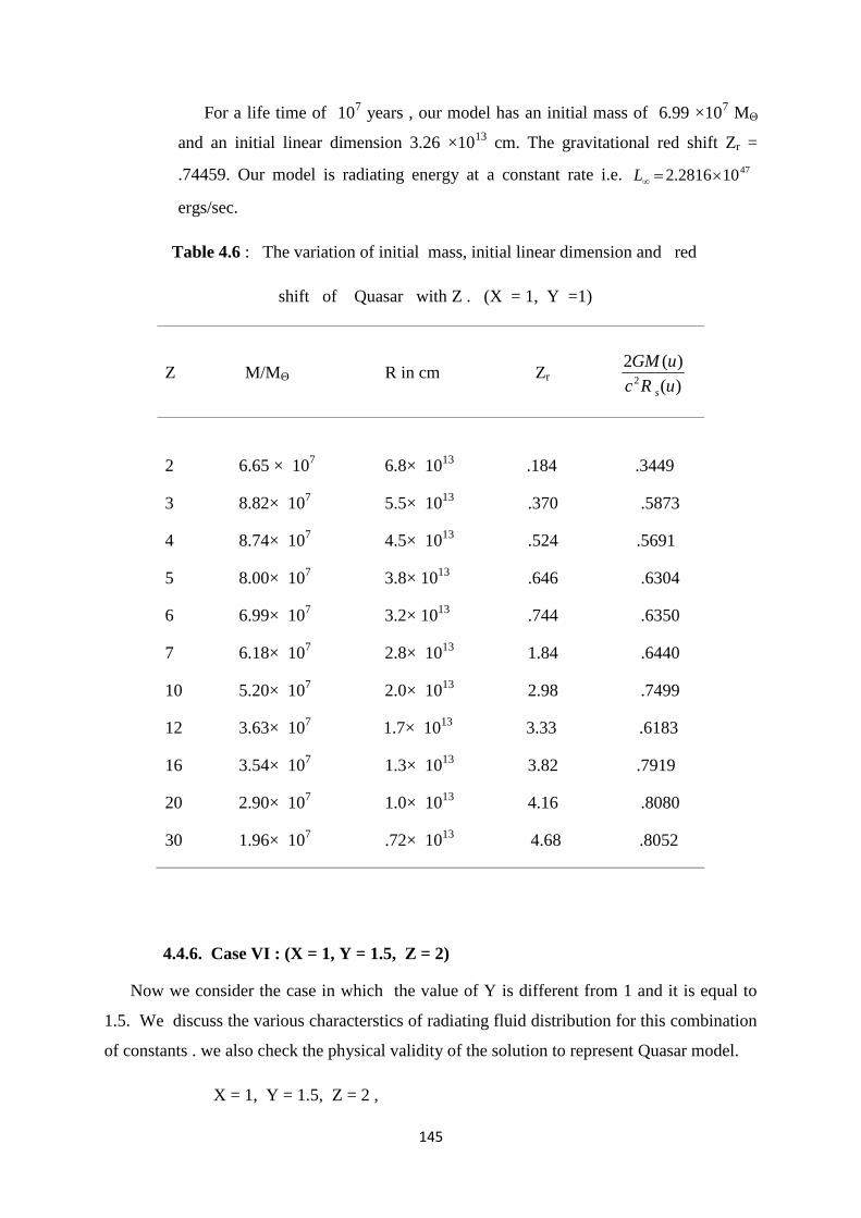
145
For a life time of 107 years , our model has an initial mass of 6.99 ×10⁷ MΘ
and an initial linear dimension 3.26 ×1013 cm. The gravitational red shift Zr =
.74459. Our model is radiating energy at a constant rate i.e. 47102816.2 L
ergs/sec.
Table 4.6 : The variation of initial mass, initial linear dimension and red
shift of Quasar with Z . (X = 1, Y =1)
Z M/MΘ R in cm Zr)(
)(22 uRc
uGM
s
2 6.65 × 10⁷ 6.8× 10¹³ .184 .3449
3 8.82× 10⁷ 5.5× 10¹³ .370 .5873
4 8.74× 10⁷ 4.5× 10¹³ .524 .5691
5 8.00× 10⁷ 3.8× 10¹³ .646 .6304
6 6.99× 10⁷ 3.2× 10¹³ .744 .6350
7 6.18× 10⁷ 2.8× 10¹³ 1.84 .6440
10 5.20× 10⁷ 2.0× 10¹³ 2.98 .7499
12 3.63× 10⁷ 1.7× 10¹³ 3.33 .6183
16 3.54× 10⁷ 1.3× 10¹³ 3.82 .7919
20 2.90× 10⁷ 1.0× 10¹³ 4.16 .8080
30 1.96× 10⁷ .72× 1013 4.68 .8052
4.4.6. Case VI : (X = 1, Y = 1.5, Z = 2)
Now we consider the case in which the value of Y is different from 1 and it is equal to
1.5. We discuss the various characterstics of radiating fluid distribution for this combination
of constants . we also check the physical validity of the solution to represent Quasar model.
X = 1, Y = 1.5, Z = 2 ,

146
rs = 0.3972
Table 4.7: The march of pressure, density, pressure-density ratio and luminosityat any instant within the ball (p in dynes cm-2, ε in g cm-3, and L in ergs s-1).
r/rs pnWc
G)(
8 224
)(
8 222
nWc
G2c
p
L
0.0 61.25 105.0 0.58 0
0.1 60.70 106.1 0.57 1.3×1045
0.2 59.06 109.7 0.54 1.0×1046
0.3 56.30 115.7 0.49 3.4×1046
0.4 52.39 124.6 0.43 8.1×1046
0.5 47.29 136.6 0.36 1.5×1047
0.6 40.91 152.3 0.28 2.6×1047
0.7 33.17 172.7 0.20 4.2×1047
0.8 23.92 198.7 0.13 6.1×1047
0.9 12.96 231.4 0.06 8.4×1047
1.0 00.00 274.8 0.00 1.1×1048
From Table 4.7 it is clear that the pressure and pressure density ratio are
monotonically decreasing with the increase of r within the radiating fluid sphere.
Luminosity is monotonically increasing with the increase of r.

147
Model of Quasar for case VII
In view of equation (4.29) ,we have
tWKtn 1526.2)( (4.66)
Consequently we have
tKWuRs 526.209728.0)( (4.67)
tWKuM 526.2102.4)( 26 (4.68)
For a life time of 107 years ,
Our model has an initial mass of 1.65 ×10⁹ MΘ,
An initial linear dimension 7.64 ×1013 cm.
The gravitational red shift Zr = . 6708
Our model is radiating energy at a constant rate i.e. 4710382.2 L ergs/sec.

148
4.4.7. Case VII : X = 1, Y = 2, Z = 2 rs = 0.4595
Table 4.8: The march of pressure, density, pressure-density ratio andluminosity at any instant within the ball.
(p in dynes cm-2, ε in g cm-3, and L in ergs s-1).
______________________________________________________________________
r/rs pnWc
G)(
8 224
)(
8 224
nWc
G2c
p
L
_____________________________________________________________________________
0.0 131.0 96.00 1.364 0
0.1 129.8 97.83 1.329 1.7×1045
0.2 126.3 103.42 1.231 1.4×1046
0.3 120.4 113.08 1.085 4.7×1046
0.4 112.1 127.35 0.911 1.1×1047
0.5 101.2 147.07 0.726 2.1×1047
0.6 87.6 173.51 0.546 3.6×1047
0.7 71.85 208.55 0.380 5.6×1047
0.8 51.46 254.99 0.233 8.2×1047
0.9 27.99 317.04 0.106 1.1×1048
1.0 00.00 401.29 0.000 1.4×1048
____________________________________________________________________________
From the Table 4.8 we observe that pressure is decreasing as we go from centre to surface ,
2c
p
is also monotonically decreasing in nature with the increase of r but it is not less than
one throughout the radiating fluid sphere. Hence it is not suitable for modeling of radiatingfluid sphere.

149
Table 4.9: Physical validity of the solution for different
combinations of X , Y and Z.
X Y Z Physically realizable
Yes /No
1 1 2, 3, 4, 5, 6, 7, Yes
1 1 10,12, 16, 20,30 Yes
2 any value any value No
1 1.5 2 Yes
1 2 2 No
1 3 2 No
1 3 3 No
4.5 Results and Discussions:
We have done an extensive study of BCT solution II [1] and have constructed
the approximate models for quasars for different combinations of constants X, Y and Z
appearing in the solution. Tables 4.1, 4.2, 4.3, 4.4, 4.5 show the variation of pressure,
density, pressure-density ratio and luminosity within the radiating fluid sphere. From these
Tables we observe that pressure, density, luminosity are positive and2c
p
< 1/3 everywhere
within the radiating balls. The pressure and pressure – density ratio are monotonically
decreasing , however luminosity is monotonically increasing with the increase of r. We have
considered the different fluid ball models of Quasar for different combinations of constants
X, Y and Z ( X =1, Y = 1, Z = 2, 3, 4, 5, 6).
The similarity of all these models is that constants X and Y are same but Z is
different for each model. Assuming the life time of quasar 107 years our models have
150
initial mass in the range of 107 MΘ with initial linear dimension in the range of 1013 cm .
From the Tables 4.1, 4.2, 4.3, 4.4, 4.5 we observe that as the value of Z increases the
pressure and density inside the radiating fluid sphere increases. In Table 4.6 the different
models of quasar have been presented for the value of Z up to 30. From Table 4.6 we
observe that the initial mass of Quasar firstly increases with Z up to Z = 4 and then
decreases. The initial linear dimension Of Quasar decreases as the value of Z increases,
however the red shift increases with the increase in the value of Z. By assigning the values
of both X and Y as 1 if we increase the value of Z from 2 onwards the solutions are
physically realizable. These solutions can be used for modeling of radiating fluid
distributions. For all these cases)(
)(22 uRc
uGM
s
< 1, hence for all the models of radiating fluid
spheres discussed above the collapse will be horizon free i.e. collapse process keeps on
going without horizon being formed in the space time. The state of naked singularity is
attained.
We have also considered the case in which Y is different from 1, i.e. case VI
( X = 1, Y = 1.5, Z = 2) . This case also gives us the physically relevant solution . Quasar
model has been constructed for the above said combination of constants. Assuming the life
time of quasar as 107 years , our model has an initial mass of 1.65 ×10⁹ MΘ, an initial linear
dimension 7.64 ×1013 cm. The gravitational red shift Zr = . 6708 and our model is radiating
energy at a constant rate i.e. 4710382.2 L ergs/sec.Table 4.7 shows the variation of
pressure, density , pressure-density ratio and luminosity within the radiating fluid ball.

151
From the Table 4.8, case VII (X = 1, Y= 2, Z = 2) we observe that pressure, energy
density, pressure –energy density ratio all are positive within the radiating fluid sphere.
Pressure, pressure-density ratio are monotonically decreasing and luminosity is increasing as
we move from centre to surface. But the pressure-density ratio is not less than 1 everywhere
within the radiating fluid sphere . Hence the combination of the constants (case VIII) is not
suitable for modeling of radiating fluid sphere. By considering the various possible
combinations among the constants X, Y, Z the physical validity of the solutions has been
shown in Table 4.9 and it may be concluded that constants X, Y, Z play a dominant role in
determining the physical validity of the radiating fluid ball models.
One interesting feature of all the models considered above is that they are
horizon free strongly favouring the existence of naked singularity. The theoretical existence
of naked singularities is important because their existence would mean that it would be
possible to observe the collapse of an object to infinite density. A naked singularity could
allow scientists to observe an infinitely dense material, which would under normal
circumstances be impossible by the cosmic censorship hypothesis. Theoretically we can say
that there is possibility of existence of naked singularity .

152
4.6 References:
[1] Tewari, B. C. : “Radiating fluid spheres in general relativity”, Astrophys.
Space Sci. 149, 233 (1988).
[2] Tewari, B. C. : “Radiating fluid distributions”, Indian J. Pure Appl. Phys.
32, 504 (1994).
[3] Pant, D. N., Tewari, B. C. : “Conformally-flat metric representing a
radiating fluid ball”, Astrophysics. Space Sci. 163, 273 (1990).
[4] Misner, C. W. : “Relativistic Equations for Spherical Gravitational
Collapse with Escaping Neutrinos”, Phys. Rev. B137, 1350 (1965).
[5] Lindquist, R. W., Schwartz, R. A. , Misner, C. W. : “Vaidya's Radiating
Schwarzschild metric”, Phys. Rev. 137, B1364 (1965).
[6] Bayin, S. S. “Radiating fluid spheres in general relativity”, Phys. Rev. D
19, 2858 (1979).
[7] Herrera, L., Jimenez, J., Ruggezi, G. L. : “Evolution of radiating fluid
spheres in general relativity”, Phys. Rev. D 22, 2305 (1980).
[8] De Oliveira, A. K. G. , Santos, N. O., Kolassis, C. A. : “More about
collapse of a radiating star”, MNRAS 216, 1001 (1985).
[9] De Oliveira, A. K. G. , Santos, N. O., “Nonadiabatic gravitational
collapse”, Astrophys. J. 312, 640 (1987).
[10] De Oliveira, A. K. G. , Kolassis, C. A., Santos, N. O., “Collapse of a
radiating star revisited”, MNRAS 231, 1011 (1988).
[11] Bonnor, W. B., de Oliveira, A.K. G., Santos, N. O.: “Radiating

153
spherical collapse”, Phys.Rev. 181, 269 (1989).
[12] Kramer, D.: “Spherically symmetric radiating solution with heat flow in
general relativity”, J. Math. Phys. 33, 1458 (1992).
[13] Maharaj, S. D., Govender, M.: “Behaviour of the Kramer radiating
star”, Aust. J. Phys. 50, 959 (1997).
[14] Maharaj, S. D. ,Govender, M. : “Radiating Collapse with Vanishing
Weyl Stresses”, Int. J. mod. Phys. D14, 667 (2005).
[15] Herrera, L., Di Prisco, A. , Hernandez, Pastora, A., Santos, N. O. : “
On the role of density inhomogeneity and local anisotropy in the fate
of spherical collapse”, Phys. Lett. A 237,113 (1998).
[16] Herrera , L., LeDenmat, G., Santos, N. O., Wang, A.: “Shear-Free
Radiating Collapse and Conformal Flatness”, Int. J. Mod. Phys. D
13, 583 (2004 a).
[17] Herrera, L., Di Prisco, A., Martin, J., Ospino, J., Santosh, N.O.,
Triconis U.: “Spherically symmetric dissipative anisotropic fluids: A
general study”, Phys. Rev. D 69, 084026 (2004b).
[18] Herrera, L., Di Prisco, A., Ospino, J.: “Some analytical models of
radiating collapsing spheres”, Phys. Rev. D, 74, 044001 (2006).
[19] Herrera, L., Di Prisco, A., Carot, J.: “Frame dragging and
superenergy”, Phys. Rev. D, 76, 044012 (2007).
[20] Herrera, L., Ospino, j., Di Prisco, A., Fuenmayor, E., Troconis, O.:
“Structure and evolution of self-gravitating objects and the orthogonal
splitting of the Riemann tensor” , Phys. Rev. D 79, 064025 (2009).
[21] Herrera, L., Santosh, N.O.: “Dynamics of dissipative gravitational

154
collapse”, Phys. Rev. D 70, 084004(2004).
[22] Mitra, A.: “Why gravitational contraction must be accompanied by
emission of radiation in both Newtonian and Einstein gravity”, Phys.
Rev. D 74, 024010 (2006).
[23] Naidu, N. F., Govinder, M. : “Causal temperature profiles in horizon-
free collapse”, J. Astrophys. Astron. 28,167 (2007).
[24] Vaidya, P. C. : “Newtonian' Time in General Relativity”, Nature 171,
260 (1953).
[25] Vaidya , P. C. “Nonstatic Solutions of Einstein's Field Equations for
Spheres of fluids radiating Energy”, Phys. Rev. 83, 10 (1951).
[26] Vaidya, P. C.: “An Analytical Solution for Gravitational Collapse with
Radiation”, Astrophys. J. 144, 343 (1966).
[27] Banerjee, A., Chatterjee, S., Dadhich, N. : “Spherical Collapse with Heat
Flow and without Horizon”, Mod. Phy. Lett. A, 35,2335(2002).
[28] Pant N. , Tewari, B.C. : “Horizon-free gravitational
collapse of radiating fluid Sphere”,
Astrophysics &Space Sci. 331 (2), 645 ( 2011).
[29] Schwarzschid, M. : “Structure and Evolution of stars”,
Dover. New York (1958).

Chapter VAdiabatic Collapse of Uniform
Density Sphere with Pressure

155
Chapter VAdiabatic Collapse of Uniform Density
Sphere with Pressure5
After studying adiabatic collapse of a uniform density sphere [with Schwarzschildgeometry in the exterior] using baryon conservation law and no-heat-transfercondition it is concluded that a uniform density sphere [with Schwarzschild geometryin the exterior] always collapses adiabatically with vanishing pressure. Alternatively,we can say that when the exterior geometry is defined by Schwarzschild vacuumsolution then the solution given by Oppenheimer and Snyder (1939)[1] is the onlyvalid solution for the collapse of a uniform density sphere.
5A part of this chapter has been published in Journal of Modern Physics
1 , 143 (2010).
156
5.1 Introduction
After a star has exhausted its nuclear fuel, it can no longer remain in
equilibrium and must undergo gravitational collapse. During gravitational collapse the
physical conditions within the star does not remain same. There are some drastic changes
that takes place within the star. We have examined the various conditions under which the
pressure within the collapsing sphere will vanish.
Radial adiabatic motion of perfect fluid spheres of uniform density, E = E(t),
but non-uniform pressure were discussed by Bonnor and Faulkes [2], Thompson and
Whitrow [3-4] and Bondi [5] under various assumed relationships between central pressure
and density. These authors discussed the problem of collapse and bounce under two
assumptions: first, that the motion is isotropic or shear-free; and second, that the density is
uniform. But Mishra and Shrivastava [6] showed that the condition of uniform density and
regularity at the centre necessarily lead to the isotropic motion. The problem of collapse of a
dust ball has been studied in detail by Durgapal and Pandey [7 ] and they have shown that
there will be no material pressure within the ball as observed by a comoving observer,
although for an external observer there will be material pressure in the ball. It has been also
discussed by Mitra[8] that matter within a collapsing homogeneous sphere is bound to be a
dust (p = 0). We have also shown that the matter with in a collapsing homogeneous sphere
will be dust or pressure will vanish witnin the sphere.
The theme of our work is rather different from that of the other authors. We have
examined whether the pressure can remain finite or not. We have considered the no-heat
transfer (NHT) conditions and baryon conservation law during the collapse. It is shown that
if the fluid is isentropic or (and) the surface temperature remains constant during the collapse
the pressure cannot remain finite (it vanishes). On the other hand if the fluid is neither
isentropic nor the surface temperature remains constant during the collapse, then the results
obtained by earlier authors (Bondi [5]) are found to be inconsistent with the baryonic
conservation and NHT condition.

157
5.2 The metric and uniform density sphere:
Vanishing shear implies that we can simultaneously introduce isotropic and co-moving
coordinates
ds2 y 2dt 2 R2(dr 2 r2d 2) (5.1)
2222 sin),,(),,( dddtrRRtryy
It is assumed that the fluid’s viscosity vanishes, and the adiabatic flow condition makes T10
component of energy momentum tensor vanish in the co-moving coordinates. The energy
momentum tensor can thus be written as
)( PgUUEPT (5.2)
Where E and P are energy density and pressure, respectively;
and the four-velocity will be given by
U (y,0,0,0) (5.3)
The hydrodynamic equations,
T; 0 and
UT; 0 , and the equation of baryon
conservation,
(nU ); 0 (Where n = number density) give us (Misner and Sharp[9],
Demianski [10])
( y /y) P /(P E) (5.4)
And
Us, 0 or s 0 and s 0 (5.5)
.t.ation w.r.differentipartial)(;.tr..ation wdifferentipartial)( tr
5.3 The boundary condition and thermodynamic relation.
For the exterior solution some authors have chosen Schwarzschild vacuum
solution while others have chosen Vaidya’s radiative solutions in the exterior.
In the later case the heat flow is given by Kramer [11].
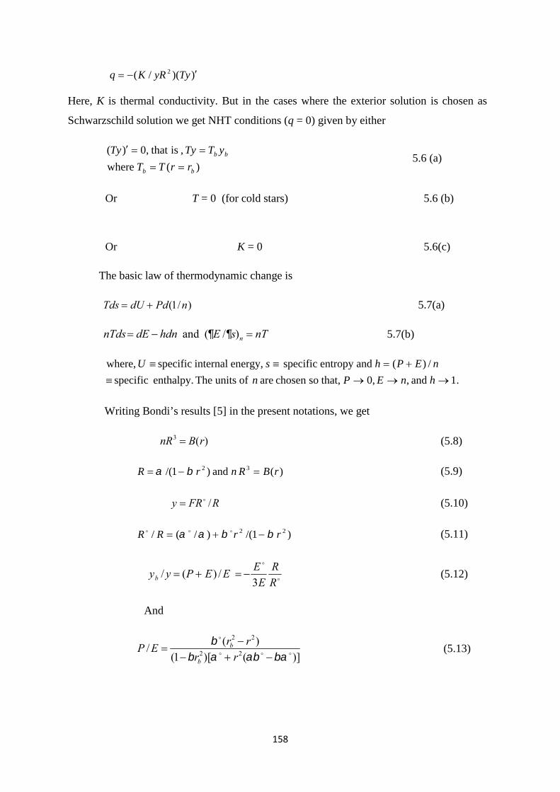
158
))(/( 2 TyyRKq
Here, K is thermal conductivity. But in the cases where the exterior solution is chosen as
Schwarzschild solution we get NHT conditions (q = 0) given by either
)(where
,is that,0)(
bb
bb
rrTT
yTTyTy
5.6 (a)
Or T = 0 (for cold stars) 5.6 (b)
Or K = 0 5.6(c)
The basic law of thermodynamic change is
Tds dU Pd(1/n) 5.7(a)
nTds dE hdn and (E /s)n nT 5.7(b)
.1and,,0 that,sochosenareofunitsTheenthalpy.specific
/)(andentropyspecificenergy,internalspecificwhere,
hnEPn
nEPhsU
Writing Bondi’s results [5] in the present notations, we get
nR3 B(r) (5.8)
)(and)1/( 32 rBRnrR (5.9)
y FR /R (5.10)
)1/()/(/ 22 rrRR (5.11)
yb / y (P E) /E E
3ERR
(5.12)
And
P /E (rb2 r2)
(1rb2)[ r2( )]
(5.13)
159
(t), (t), F F(t), yb y(r rb ), rb r at the boundary.
Since
E E (t) or E 0 , we write [using equation 5.7(b)]
(5.15)(5.12)]equation[using)/(
(5.14))/()/( 2
sEyTy
EPsTnn
b
5.4 Collapse of uniform density sphere
The collapse of uniform density sphere is discussed under various physical conditions. [We
have assumed that ttA offunctionarbitraryany)( and B(r)
any arbitrary function of r]
5.4(a) using NHT condition given by eq. (5.6a):
Using equation 5.6 (a) in (5.15) we get ,
(5.16))(1)/(
or)/(/ 2
bb
b
ssTnE
sETnn
)( bb rrss .
It is obvious from equation (5.16) that the entropy of an adiabatic uniform density sphere is
minimum at the boundary.
5.4(b) : Isentropic case: Let the entropy be constant throughout the sphere, that is, s
= constant = sb. Equation (5.16) gives
E = n (5.17)
[Using equation (5.8)] )(3 rBER
)()( rBtAR (5.18)
)(/ tARR
[From equation (5.10)] y = )(tA , or
160
0y (5.19)
[From equation (5.4)] 0P , or
)(tPP (5.20)
Since, )(0)( tPrrP b , the pressure vanishes within the sphere. Hence, an isentropic
uniform sphere undergoes a collapse with vanishing pressure only.
5.4 (c) Non-isentropic case with constant surface temperatures: We
assume that the surface temperature remains constant during the collapse. This is very likely
because there is no energy loss to the surrounding from the surface of the sphere. With Tb =
constant during the collapse one gets
n E /[1 Tb (s sb )] A(t)B(r) (5.21)
[From equation (5.8)]
R A ( t ) B (r ) (5.22)
Arguments similar to those in 5.4(b) show that the pressure vanishes inside thesphere.
Hence, an adiabatic uniform density sphere with constant surface temperature
collapses with vanishing pressure.
5.4(d) General case: Neither the fluid is isentropic nor the temperature of the
surface remains constant. In this case
E n[1 Tb (s sb )] (5.23)
On differentiating with respect to time we obtain
E
En
nTb(s sb )
1 Tb (s sb )(5.24)
For an adiabatic motion the total mass energy is a constant of motion,
that is,
M (4 /3)ERb3 constant
Or
E /E 3Rb /R (5.25)

161
Using equations (5.8), (5.11), (5.24), and (5.25) we get
22222
22
22
22
2
2
2
2
)(1
)(3
)1()1(
)(3
1
3
1
3
)(1
)(
bb
b
b
b
b
b
bb
bb
rrrr
rr
rr
rr
r
r
r
r
ssT
ssT
(5.26)
No choice of functions
s s(r), (t) and Tb Tb (t) can satisfy this equation. The
solutions obtained by various authors for collapsing/expanding uniform density
[with Schwarzschild exterior solutions] are inconsistent with the conservation law
and NHT .
5.5 Explanation of inconsistency:
Equation 5.7(b) shows that
(E /s)n nT
but from equation (5.16) we see that
(E /s)n nTb . Therefore,
nT nTb or T Tb . Since,
Ty Tbyb [from equation (5.6 a)] we get
y yb A(t).
Hence,
0)(
0(5.4)]equation[fromor0
brrPP
Py
The pressure vanishes throughout the sphere.
5.5(a) using NHT condition given by eq. 5.6(b):
When T = 0 equation (5.14) gives )(or0 tnnn
or,
R A ( t ) B (r ) [from equation (5.8)]. As shown in 5.4(b) the pressure
vanishes inside the sphere.
5.5 (b) using NHT condition given by eq. 5.6(c):
When thermal conductivity K = 0, it seems that all the relations of Bondi’s paper are
inconsistent . However, let us analyse this condition in some details. From equation (5.7 b)
we can see that
n /n E /(P E) and n /n E /(P E) (T /h) s (5.27)
162
And for
E E ( t ) ,
(T /h) s n /n (5.28)
When K = 0, no heat enters or leaves any layer within the structure during the
collapse that is we can consider temperature of each layer to be independent of time
or
T = T (r).
Eliminating n from the twin equations (5.27) we obtain [11]
Th
s E P P EP E
0
E PP E
for E E(t)(5.29), or
nT (T /h)P E ( P / s ) (5.30)
It can be seen from equation (5.13), that the right hand side of equation (5.30) cannot be
made zero in any case.
Now, we consider a hypothetical case that during the collapse, though K = 0,
somehow the temperature of each layer changes with time making
T T ( r, t ) , but at the
surface the temperature will not change with time, that is,
Tb 0 . It can be seen that
brrb TPsPEET )/( (5.31)
The right hand side of equation (5.31) cannot be made zero.
5.6. Results & Discussions
After studying adiabatic collapse of a uniform density sphere [with
Schwarzschild geometry in the exterior] using baryon conservation law and NHT
condition it is concluded that,
(i) If the fluid (with
K 0 ) is isentropic or (and) the sphere’s surface temperature
remains constant during the collapse, then the pressure vanishes inside the sphere.

163
(ii) If neither the fluid (with
K 0 ) is isentropic nor the surface temperature of the
sphere remains constant during the collapse the solution obtained by Bondi (1969)
and other authors are found to be inconsistent with the baryonic conservation and
NHT condition. Moreover, it is again seen that the pressure vanishes.
(iii) If the temperature is zero (cold stars) the pressure vanishes inside the
configuration.
(iv) If
K 0 , we can show that the pressure vanishes throughout the sphere.
Thus, we conclude that a uniform density sphere [with Schwarzschild geometry
in the exterior] always collapses adiabatically with vanishing pressure. The matter
with in a collapsing homogeneous sphere is bound to be dust (p = 0). Or we can say
that when the exterior geometry is defined by Schwarzschild vacuum solution then
the solution given by Oppenheimer and Snyder [1] is the only valid solution for the
collapse of a uniform density sphere.

164
5.7 References:
[1] Oppenheimer, J. R. and Snyder, H.: “On Continued Gravitational
Contraction” , Phy. Rev. 56, 455(1939).
[2] Bonnor , W. B. and Faulkes, M. C. : “Exact Solutions for Oscillating
Spheres in General Relativity”, Mon. Not. R. astr. Soc. 137 239
(1967).
[3] Thompson, I. H. and Whitrow, G. J.: “Time-Dependent Internal
Solutions for Spherically Symmetrical Bodies in General
Relativity-I. Adiabatic collapse”, Mon. Not. R.astr.Soc. 136 208(1967).
[4] Thompson, I. H. and Whitrow, G. J.: “Time-dependent internal
solutions for spherically symmetrical bodies in general relativity-II.
Adiabatic radial motions of uniformly dense spheres”, Mon. Not. R.
Astr. Soc. 139,499(1968).
[5] Bondi, H. : “Gravitational Bounce in General Relativity”, Mon. Not.
R. Astr. Soc. 142 333(1969).
[6] Misra, R. M. and Srivastava, D. C.: “Relativity-Bounce of Fluid
Spheres”, Nature 238, 116(1972).
[7] Durgapal M. C. and Pande A. K. : “Gravitational Collapse of a dust
ball- The external point of view” ,Astrophysics &Space Science
116, 349 1985.
[8] Mitra, A. : “The matter in the Big-Bang model is dust and not any
arbitrary perfect fluid”, Astrophysics & Space Science DOI
10.1007/s10509-011- 0635-8(2011).
165
[9] Misner, C.W. and Sharp, D. H. : “Relativistic Equations for
Adiabatic, Spherically Symmetric Gravitational Collapse” , Phys.
Rev. B, 136, 571(1964).
[10] Demianski, M.: “Relativistic Astrophysics”, (Pergamon Press)
New York 188(1985).
[11] Kramer, D.: “Spherically Symmetric Radiating Solution with Heat
Flow in General Relativity” , J. Math. Phys. 33 (4), 1458(1992).
[12] Nariai, H.: “A Simple Model for Gravitational Collapse with
Pressure Gradient”, Progress of Theoretical physics 38
,92 (1967).

Chapter VIA New Time Dependent solution of
Einstein’s field equations
&
Radiating fluid balls in conformallyflat space-time.
166
CHAPTER VI
A new time dependent solution of Einstein’s field equations&Radiating fluid balls in conformally flat space-time.
In this chapter we have obtained a new time dependent solution of Einstein field
equations . we have discussed various conditions under which the B.C.T. solution [1] in
conformally flat space time region will be suitable for the modeling of radiating stellar
objects . The variation of pressure, density, pressure-density ratio , luminosity from centre to
surface have been studied. With suitable choice of constants appearing in the solution we
have shown that pressure, density, luminosity, pressure-density ratio all are positive with in
the radiating fluid ball. It has been also shown that as the time will evolve the pressure and
density will also tend to increase indicating that the astrophysical object will move towards
more and more compact stage.

167
6.1 Introduction:
To study the astrophysical objects emitting a large amount of energy in the form of
neutrinos and photons the non static solution of Einstein’s field equations with outflowing
radiation becomes significant. The problem of such massive stellar objects was initiated by
Vaidya [2-3] with extension of Tolman [4] taking account of out flowing radiation. We will
study the radiating fluid balls in conformally flat space time metric. In conformally flat
space-time metric there is only one variable that is to be determined by solving the field
equations.
In case of an empty space-time, a space-time conformal to the flat space time
is itself flat [5]. But in case of nonempty space-time it may not be true. The study of
nonempty space-time conformal to the flat space-time may have significance on the
radiating astrophysical objects due to the mathematical simplicity involved. Realistic
models of radiating fluid spheres in general relativity are few on account of
associated mathematical complexities. P.C. Vaidya [2-3] solved the field equation of
general relativity for physically meaningful models of radiating fluid balls. Bayin,
S. S. [6] suggested a generalization of Vaidya's metric which, designed to depict the
external field of radiating mass. Tewari, B. C. et al.[1] have considered the
spherically symmetric space time in conformally flat form which had simplified the
field equation to a great extent. Jasim et al. [7] reconsidered the spherically
symmetric metric in conformally flat form and obtained a class of radiating fluid
sphere. A relativistic model of fluid sphere filled with matter and radiation has been
constructed by Jasim et al. [8]. The immense gravity objects radiate a large amount
of energy while undergoing gravitational collapse. Oppenheimer and Synder [9]
first studied gravitational collapse for spherically symmetric fluid distribution
neglecting radiation , pressure and rotation. But Vaidya [2-3] [10] gave the idea that
the gravitational collapse is a highly dissipating energy process and took into
account the outflowing radiation also while solving the Einstein’s field equations.
Thus the radiating fluid ball models may be studied by solving the Einstein’s field
equations either by using the general metric of space-time having three variable or
by using the conformally flat space-time metric having only one variable. Herrera et al.
proposed a general method for obtaining collapsing radiating models from exact

168
static solutions of Einstein’s field equations for a spherically symmetric fluid distribution.
Some of the authors studied the radiating fluid spheres with physically significant solutions
in the free streaming case (Tewari [11-13], Pant et al. [14] , Pant and Tewari [1]) by solving
the modified field equations proposed by Misner [15], Lindquist et al. [16]. We have also
studied the solution obtained by Tewari in conformally flat metric form and checked its
validity for representing the radiating fluid spheres. We have also obtained a new solution of
Einstein’s field equaions by using the general metric of space-time having three variables.
6.2 The metric and Field Equations:
For the gravitational field within the radiating fluid sphere the space time metric in three
variables is given by
22222222 sin dderdredtceds (6.1)
Where α , β , are functions of r and t.
The field equations of general relativity for a distribution of mixture of a
perfect fluid and radiation are
ji
ji
ji T
c
GgRR
4
8
2
1 (6.2)
where
jij
ij
ij
i wwc
qgpvvcpT )( 2 (6.3)
where p and respectively denote the isotropic pressure and density of the matter
within the distribution and vi its four velocity, q denotes the radiation flux density and iw its
four velocity which is null.
0ii ww (6.4)
We choose iw such that[15]
,1 11
rB
tcA
xw
ii
(6.5)
which implies that q is the energy density of the radiation in the rest frame of the fluid
[15,16]
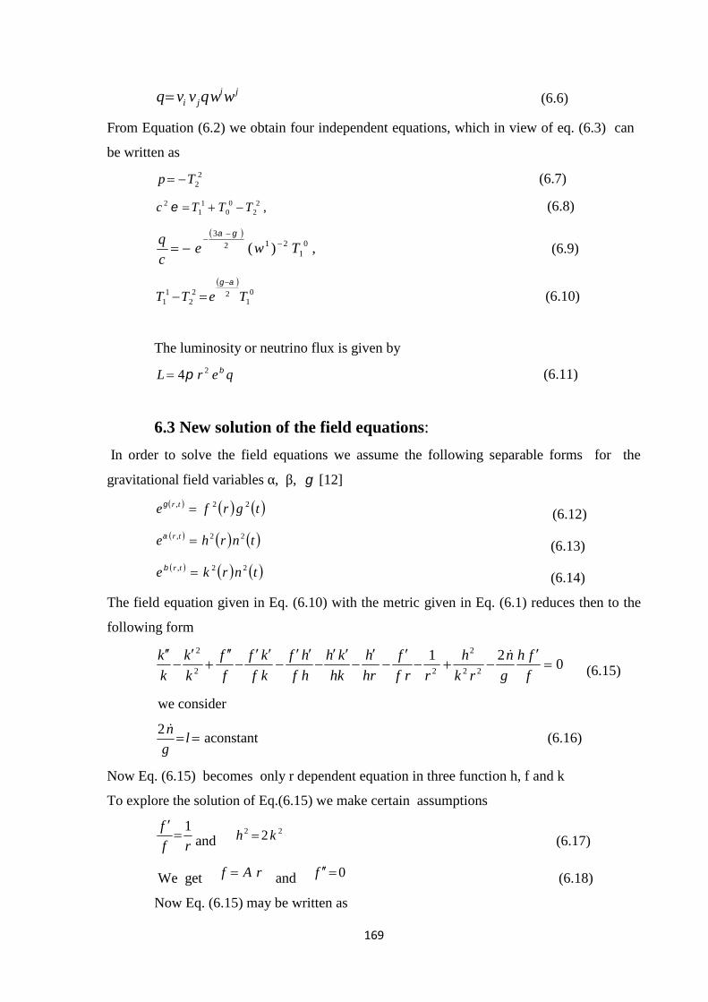
169
jiji wwqvvq (6.6)
From Equation (6.2) we obtain four independent equations, which in view of eq. (6.3) can
be written as
22Tp (6.7)
,22
00
11
2 TTTc (6.8)
,)( 0
1212
3
Twec
q
(6.9)
0
122
21
1 TeTT
(6.10)
The luminosity or neutrino flux is given by
qerL 24 (6.11)
6.3 New solution of the field equations:
In order to solve the field equations we assume the following separable forms for the
gravitational field variables α, β, [12]
tgrfe tr 22, (6.12)
tnrhe tr 22, (6.13)
tnrke tr 22, (6.14)
The field equation given in Eq. (6.10) with the metric given in Eq. (6.1) reduces then to the
following form
021
22
2
22
2
f
fh
g
n
rk
h
rrf
f
hr
h
hk
kh
hf
hf
kf
kf
f
f
k
k
k
k (6.15)
we consider
lg
n2aconstant (6.16)
Now Eq. (6.15) becomes only r dependent equation in three function h, f and k
To explore the solution of Eq.(6.15) we make certain assumptions
rf
f 1
and22 2 kh (6.17)
We get rAf and 0f (6.18)
Now Eq. (6.15) may be written as

170
0232
22
2
rA
kl
kr
k
k
k
k
k
(6.19)
or
023222
rA
l
k
k
rk
k
(6.20)
The solution of Eq.(6.20) is written as follows :
14
4log
4
2
C
Brr
A
lk
(6.21)
14
4log
4
22
C
Brr
A
lh
(6.22)
Where A, B, C are integration constants.
Assuming t as the proper time of the distant observer at rest on the hyper surface
rs we have
1)()( 22 tgrf s (6.23)
From Eq. (6.18) and Eq. (6.23) we obtain
srA
tg1
(6.24)
The expression for n(t) is obtained as
trA
clKtn
s2)(
(6.25)
Where K is a non negative constant.
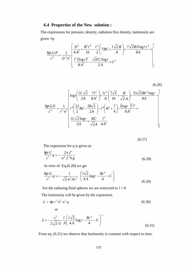
171
6.4 Properties of the New solution :
The expressions for pressure, density, radiation flux density, luminosity are
given by
2
2
22
4482
2
2
224
2
log2
8
log
8
log2727
2164
3
2
18
CA
rCl
A
rl
A
rrlB
A
BlBC
rrB
A
l
nrc
PG
(6.26)
2
2
2
22
284
44
2
2
224
42
3
2
log2
8
log
4
7
2
2
2
21
8
log221
216
27
8
7
2
2log
18
A
l
A
lC
A
rCl
A
lrBr
A
lBBCr
A
rlBr
A
B
A
rl
A
l
A
Clr
nrc
EG
(6.27)
The expression for q is given as
ghfn
fnq
c
G225
28
(6.28)
In view of Eq.(6.28) we get
C
Brr
A
l
rAn
lq
c
G
4log
4
2
2
8 4
225
(6.29)
For the radiating fluid spheres we are restricted to 0l
The luminosity will be given by the expression
qnkrL 2224 (6.30)
or
145
4log
4
2
22
C
Brr
A
l
A
l
G
cL
(6.31)
From eq. (6.31) we observe that luminosity is constant with respect to time.
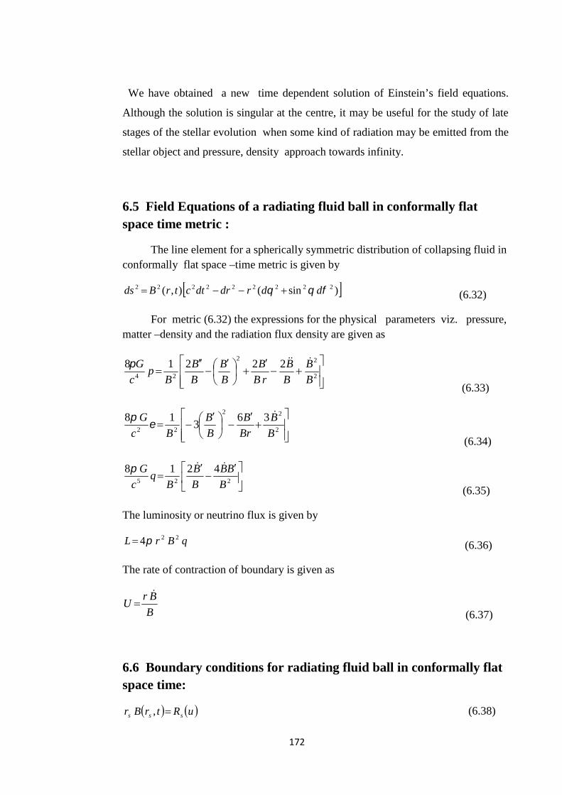
172
We have obtained a new time dependent solution of Einstein’s field equations.
Although the solution is singular at the centre, it may be useful for the study of late
stages of the stellar evolution when some kind of radiation may be emitted from the
stellar object and pressure, density approach towards infinity.
6.5 Field Equations of a radiating fluid ball in conformally flatspace time metric :
The line element for a spherically symmetric distribution of collapsing fluid inconformally flat space –time metric is given by
)sin(),( 222222222 ddrdrdtctrBds (6.32)
For metric (6.32) the expressions for the physical parameters viz. pressure,matter –density and the radiation flux density are given as
2
22
24
22218
B
B
B
B
rB
B
B
B
B
B
Bp
c
G
(6.33)
2
22
22
363
18
B
B
Br
B
B
B
Bc
G
(6.34)
225
4218
B
BB
B
B
Bq
c
G
(6.35)
The luminosity or neutrino flux is given by
qBrL 224 (6.36)
The rate of contraction of boundary is given as
B
BrU
(6.37)
6.6 Boundary conditions for radiating fluid ball in conformally flatspace time:
uRtrBr sss , (6.38)

173
s
s B
Br
B
BrdudtctrB
1, (6.39)
0, trp s (6.40)
s
s B
BrBr
B
Br
G
ctrmuM
22,
232
232
(6.41)
The expression for L∞ is given as
2
1s
s B
Br
B
BrLL
(6.42)
Now we study the solution obtained by Tewari [1] in conformally flat space time.
The general solution of the field equation as obtained by Tewari[1] is
1)(
drctrfrtGB(6.43)
The particular solution obtained is [1]
)( ctrbectrf and )()( ctrb sehtG (6.44)
where b is a constant and h is a nonnegative constant satisfying the followingrelation:
0342 3224 srhbhbhb (6.45)
From which the following relation is obtained
hb
hbhbrs 3
224
4
32
(6.46)
The expression for pressure , matter density, and radiation flux density are obtainedas[1]
ss rbrrbbrbct ehbebrheb
epc
G 222)(22
24
)21(238
(6.47)
ss rbrrbbrbct ehbebrhe
be
c
G 222)(22
22
3638
(6.48)
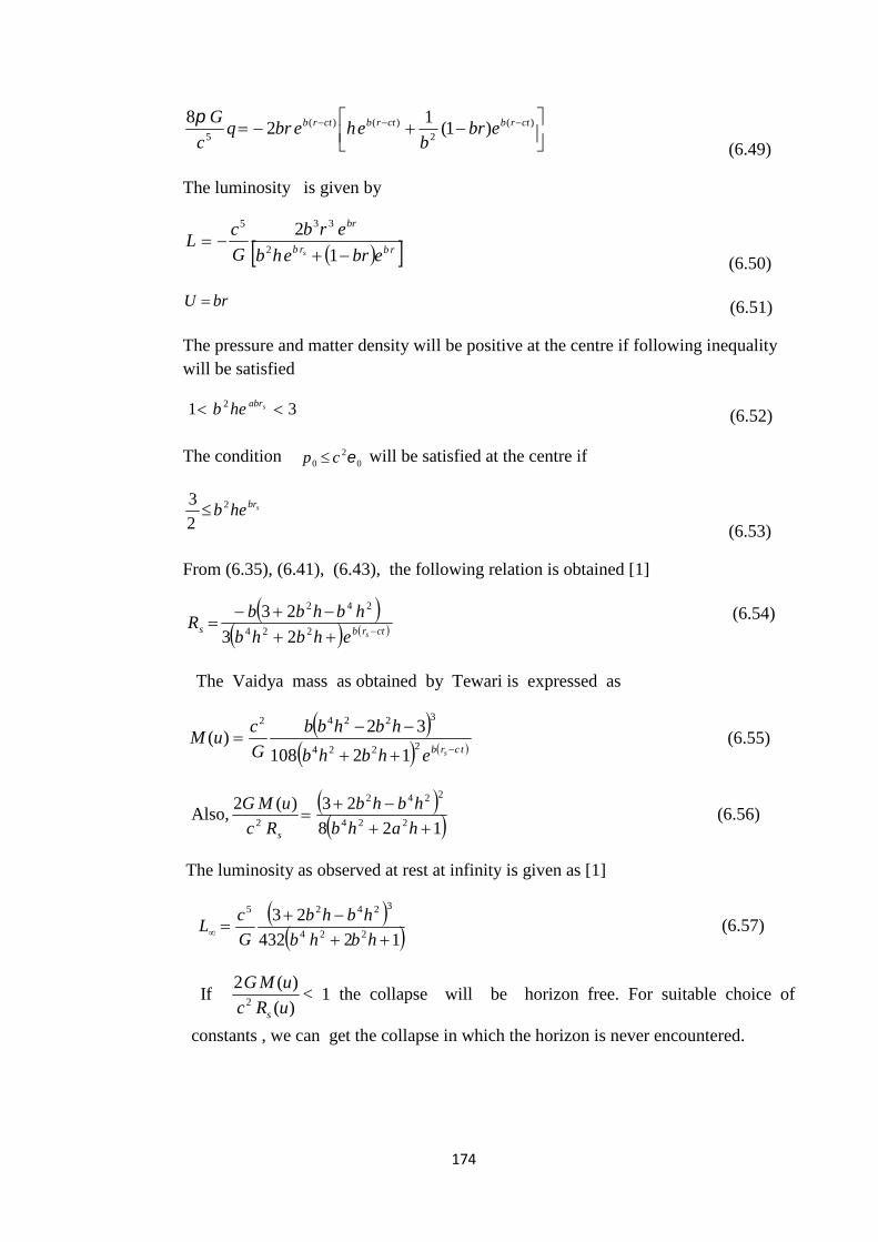
174
)(
2)()(
5)1(
12
8 ctrbctrbctrb ebrb
ehebrqc
G
(6.49)
The luminosity is given by
rbrb
br
ebrehb
erb
G
cL
s
1
22
335
(6.50)
brU (6.51)
The pressure and matter density will be positive at the centre if following inequalitywill be satisfied
31 2 sabrheb (6.52)
The condition 02
0 cp will be satisfied at the centre if
sbrheb 2
2
3
(6.53)
From (6.35), (6.41), (6.43), the following relation is obtained [1]
(6.54)
The Vaidya mass as obtained by Tewari is expressed as
tcrb sehbhb
hbhbb
G
cuM
2224
32242
12108
32)( (6.55)
Also, 128
23)(2224
2242
2
hahb
hbhb
Rc
uMG
s
(6.56)
The luminosity as observed at rest at infinity is given as [1]
12432
23224
32425
hbhb
hbhb
G
cL (6.57)
If)(
)(22 uRc
uMG
s
< 1 the collapse will be horizon free. For suitable choice of
constants , we can get the collapse in which the horizon is never encountered.
ctrbs
sehbhb
hbhbbR
224
242
23
23
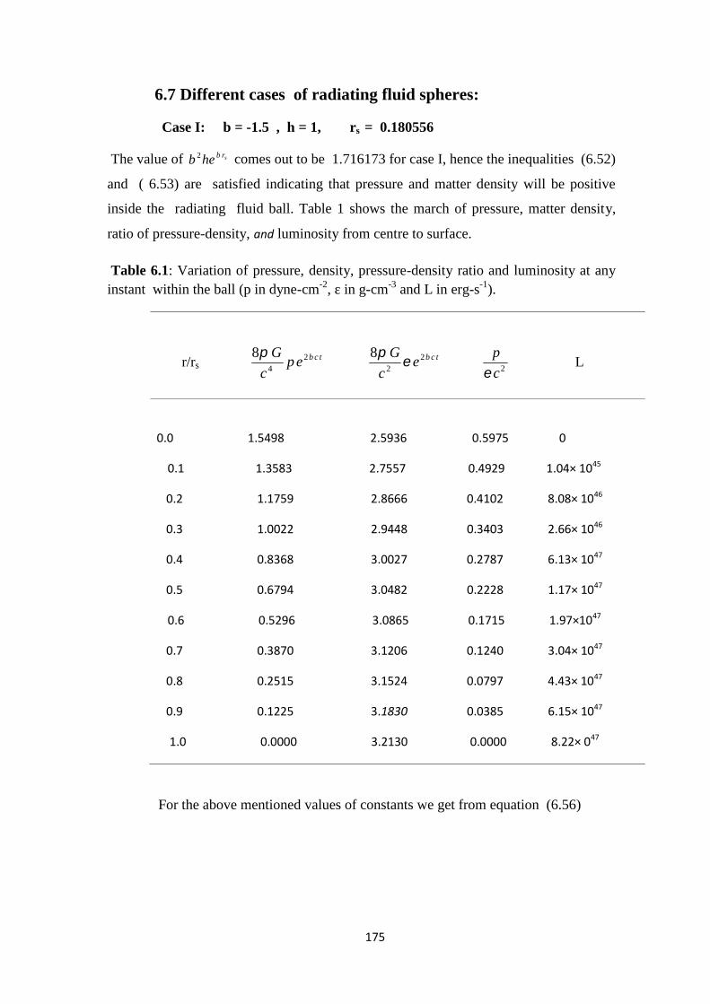
175
6.7 Different cases of radiating fluid spheres:
Case I: b = -1.5 , h = 1, rs = 0.180556
The value of srbheb 2 comes out to be 1.716173 for case I, hence the inequalities (6.52)
and ( 6.53) are satisfied indicating that pressure and matter density will be positive
inside the radiating fluid ball. Table 1 shows the march of pressure, matter density,
ratio of pressure-density, and luminosity from centre to surface.
Table 6.1: Variation of pressure, density, pressure-density ratio and luminosity at anyinstant within the ball (p in dyne-cm-2, ε in g-cm-3 and L in erg-s-1).
r/rstcbep
c
G 24
8 tcbec
G 22
8
2c
p
L
0.0 1.5498 2.5936 0.5975 0
0.1 1.3583 2.7557 0.4929 1.04× 1045
0.2 1.1759 2.8666 0.4102 8.08× 1046
0.3 1.0022 2.9448 0.3403 2.66× 1046
0.4 0.8368 3.0027 0.2787 6.13× 1047
0.5 0.6794 3.0482 0.2228 1.17× 1047
0.6 0.5296 3.0865 0.1715 1.97×1047
0.7 0.3870 3.1206 0.1240 3.04× 1047
0.8 0.2515 3.1524 0.0797 4.43× 1047
0.9 0.1225 3.1830 0.0385 6.15× 1047
1.0 0.0000 3.2130 0.0000 8.22× 047
For the above mentioned values of constants we get from equation (6.56)
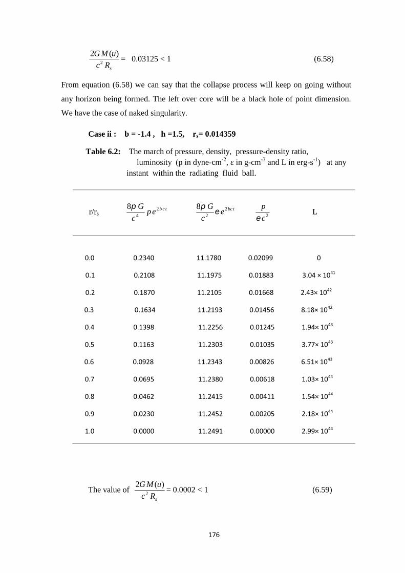
176
sRc
uMG2
)(2= 0.03125 < 1 (6.58)
From equation (6.58) we can say that the collapse process will keep on going without
any horizon being formed. The left over core will be a black hole of point dimension.
We have the case of naked singularity.
Case ii : b = -1.4 , h =1.5, rs= 0.014359
Table 6.2: The march of pressure, density, pressure-density ratio,luminosity (p in dyne-cm-2, ε in g-cm-3 and L in erg-s-1) at any
instant within the radiating fluid ball.
r/rstcbep
c
G 24
8 tbcec
G 22
8
2c
p
L
0.0 0.2340 11.1780 0.02099 0
0.1 0.2108 11.1975 0.01883 3.04 × 1041
0.2 0.1870 11.2105 0.01668 2.43× 1042
0.3 0.1634 11.2193 0.01456 8.18× 1042
0.4 0.1398 11.2256 0.01245 1.94× 1043
0.5 0.1163 11.2303 0.01035 3.77× 1043
0.6 0.0928 11.2343 0.00826 6.51× 1043
0.7 0.0695 11.2380 0.00618 1.03× 1044
0.8 0.0462 11.2415 0.00411 1.54× 1044
0.9 0.0230 11.2452 0.00205 2.18× 1044
1.0 0.0000 11.2491 0.00000 2.99× 1044
The value ofsRc
uMG2
)(2= 0.0002 < 1 (6.59)
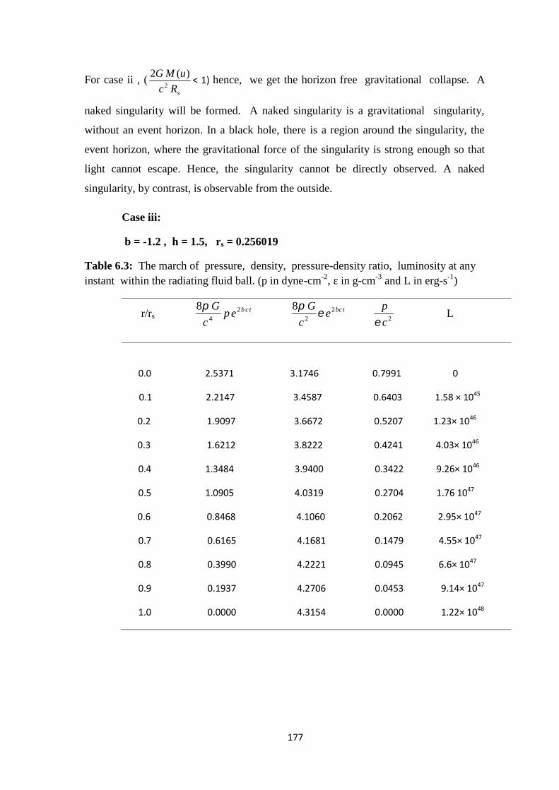
177
For case ii , (sRc
uMG2
)(2 < 1) hence, we get the horizon free gravitational collapse. A
naked singularity will be formed. A naked singularity is a gravitational singularity,
without an event horizon. In a black hole, there is a region around the singularity, the
event horizon, where the gravitational force of the singularity is strong enough so that
light cannot escape. Hence, the singularity cannot be directly observed. A naked
singularity, by contrast, is observable from the outside.
Case iii:
b = -1.2 , h = 1.5, rs = 0.256019
Table 6.3: The march of pressure, density, pressure-density ratio, luminosity at anyinstant within the radiating fluid ball. (p in dyne-cm-2, ε in g-cm-3 and L in erg-s-1)
r/rstcbep
c
G 24
8 tbcec
G 22
8
2c
p
L
0.0 2.5371 3.1746 0.7991 0
0.1 2.2147 3.4587 0.6403 1.58 × 1045
0.2 1.9097 3.6672 0.5207 1.23× 1046
0.3 1.6212 3.8222 0.4241 4.03× 1046
0.4 1.3484 3.9400 0.3422 9.26× 1046
0.5 1.0905 4.0319 0.2704 1.76 1047
0.6 0.8468 4.1060 0.2062 2.95× 1047
0.7 0.6165 4.1681 0.1479 4.55× 1047
0.8 0.3990 4.2221 0.0945 6.6× 1047
0.9 0.1937 4.2706 0.0453 9.14× 1047
1.0 0.0000 4.3154 0.0000 1.22× 1048

178
For the case (iii) we get
0196.0)(2
2
sRc
uMG< 1 (case of naked simgularity) (6.60)
Case iv: b = -1 , h = 2.5, rs = 0.175
Table 6.4: The march of pressure, density, pressure-density ratio, luminosity atany instant with in the radiating fluid ball. (p in dyne-cm-2, ε in g-cm-3 and L inerg-s-1)
r/rstbcep
c
G 24
8 tbcec
G 22
8
2c
p
L
0.0 2.7929 10.2129 0.2734 0
0.1 2.4726 10.4965 0.2555 2.48 × 1044
0.2 2.1620 10.7111 0.2018 1.95× 1045
0.3 1.8611 10.8747 0.1711 6.46 × 1045
0.4 1.5694 11.0008 0.1426 1.51× 1046
0.5 1.2867 11.0998 0.1159 2.89× 1046
0.6 1.0127 11.1793 0.0905 4.91× 1046
0.7 0.7474 11.2451 0.0664 7.67× 1046
0.8 0.4902 11.3014 0.0433 1.1 × 1047
0.9 0.2412 11.3513 0.0212 1.58× 1047
1.0 0.0000 11.3970 0.0000 2.13× 1047
For the case iv we get
sRc
uMG2
)(2= 0.01388 < 1 (6.61)
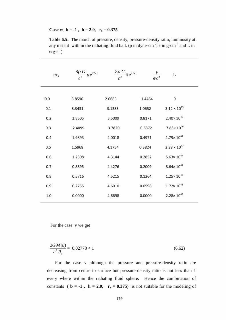
179
Case v: b = -1 , h = 2.0, rs = 0.375
Table 6.5: The march of pressure, density, pressure-density ratio, luminosity atany instant with in the radiating fluid ball. (p in dyne-cm-2, ε in g-cm-3 and L inerg-s-1)
r/rstbcep
c
G 24
8 tbcec
G 22
8
2c
p
L
0.0 3.8596 2.6683 1.4464 0
0.1 3.3431 3.1383 1.0652 3.12 × 1045
0.2 2.8605 3.5009 0.8171 2.40× 1046
0.3 2.4099 3.7820 0.6372 7.83× 1046
0.4 1.9893 4.0018 0.4971 1.79× 1047
0.5 1.5968 4.1754 0.3824 3.38 × 1047
0.6 1.2308 4.3144 0.2852 5.63× 1047
0.7 0.8895 4.4276 0.2009 8.64× 1047
0.8 0.5716 4.5215 0.1264 1.25× 1048
0.9 0.2755 4.6010 0.0598 1.72× 1048
1.0 0.0000 4.6698 0.0000 2.28× 1048
For the case v we get
sRc
uMG2
)(2= 0.02778 < 1 (6.62)
For the case v although the pressure and pressure-density ratio are
decreasing from centre to surface but pressure-density ratio is not less than 1
every where within the radiating fluid sphere. Hence the combination of
constants ( b = -1 , h = 2.0, rs = 0.375) is not suitable for the modeling of

180
radiating fluid spheres. Similarly for other combinations of constants b and h
the solution is not well behaved , hence not suitable for modeling of radiating
fluid spheres.
6.8 The behaviour of pressure and density w. r. t. time
Differentiating equation (6.47) we get
ss rbrrbbrbct ehbebrheb
bcepc
G 222)(22
24
)21(23
28
(6.63)
Differentiating equation (6.63) again we get
ss rbrrbbrbct ehbebrheb
ecbpc
G 222)(22
2224
)21(23
48
(6.64)
From Eq. (6.64) it is clear that pressure will increase with time.
Similarly if we differentiate equation (6.48) we get
ss rbrrbbrbct ehbebrhe
bbce
c
G 222)(22
22
363
28
(6.65)
Differentiating equation (6.65) again we get
ss rbrrbbrbct ehbebrhe
becb
c
G 222)(22
2222
363
48
(6.66)
In view of equation (6.65) and ( 6.66) we can say that the density will increasewith time. As the time will evolve, the pressure and density will tend towardsinfinity.
181
6.9 Results and Discussions:
We have obtained a new time dependent solution of Einstein’s field equations in
general metric form using three variables. The expressions for pressure, energy density,
luminosity and radiation flux density have been obtained. Although the solution is
singular at the centre it may give some insight in understanding certain stages of
radiating stars. We have also studied a known non static solution of Einstein’s field
equations in conformally flat space time which was obtained by Tewari [1]. The
different cases of radiating fluid ball have been considered for the different
combination of constants. The constants have been chosen in such a way , so that the
inequalities (6.52) and ( 6.53) may get satisfied. From the Tables 6.1, 6.2, 6.3 , 6.4 and
6.5 we observe that the pressure , pressure density ratio decrease as we go from centre to
surface and pressure becomes zero at the boundary. Luminosity increases as we go
from centre to surface. Tables 6.1, 6.2, 6.3, 6.4 show that the value of pressure-density
ratio is less than one within the radiating fluid sphere. But in the Table 6.5
corresponding to case v we observe that although pressure and pressure-density ratio is
decreasing from centre to surface, but pressure-density ratio is not less than 1
everywhere within the radiating fluid sphere. Hence case v can not be considered a
realistic case for radiating fluid ball problem. One important parameter that we have
investigated for all these models issRc
uMG2
)(2. We observe that for all the four cases
sRc
uMG2
)(2< 1, which indicates that collapse will be horizon free and naked singularity
may come into existence. If the horizon is formed during the collapse we will be
deprived of the events happening inside the horizon.
From equations (6.47) and (6.48) it is evident that with the passage of time both
the pressure and density will tend towards infinity and we will come towards more
and more compact stage. In this way the solution obtained in conformally flat metric
case [1] may be applied for constructing the radiating fluid ball models.

182
6.10 References :
[1] Pant, D. N., Tewari, B. C. : "conformally flat metric representing a
radiating fluid ball", Astrophysics. Space Sci. 163, 223 (1990).
[2] Vaidya, P.C.: “Non-static solutions of Einstein's field equations for
spheres of fluid radiating energy”, Phys. Rev. 83, 10 (1951).
[3] Vaidya, P. C.: “Newtonian Time in General Relativity”, Nature
171, 260 (1953).
[4] Tolman, R. C.: “Static solutions of Einstein’s field equations for
spheres of fluid”, Phys. Rev. 55 ,364 (1939).
[5] Singh, K. P. and Roy, S. R. : Proc. Nat. Inst. Sci. India, 32, 223
(1966).
[6] Bayin, S. S.: “Radiating fluid spheres in general relativity”,
Phys. Rev. D 19, 2858 (1979).
[7] Jasim, M. K. et al., On conformally-flat radiating fluid
spheres", Proceeding of GR15, Dec. 16-21, IUCAA, Pune, India,
(1997).
[8] Jasim, M. K. et al. : “A New Generating Solution of a Relativistic
Radiating Fluid Spheres Model”, Applied Mathematical Sciences,
5(80),4005 (2011).
[9] Oppenheimer, J. R . and Snyder, H . : “On Continued Gravitational
Contraction” , Phy. Rev. 56, 455(1939).
[10] Vaidya, P.C.: “An analytical solution to gravitational collapse with
radiation” , Astrophys. J. 144, 343 (1966).

183
[11] Tewari, B.C. : “Radiating fluid spheres in general relativity”,
. Space sci. 149, 233 (1988).
[12] Tewari, B. C.: “Relativistic radiating fluid distribution”, Indian J.
Appl. Phys. 32,504 (1994).
[13] Tewari, B. C.: “Relativistic model for radiating star”,
Astrophys.Space Sci. 306, 273 (2006).
[14] Pant, N. , Tewari, B.C.: “Horizon-free gravitational collapse of
radiating fluid sphere”, 331(2), 645 (2011).
[15] Misner, C. W.: “Relativistic Equations for Spherical
Gravitational Collapse with Escaping Neutrinos”, Phys. Rev.
B137, 1350 (1965).
[16] Lindquist, R .W., Schwartz, R. A. , Misner, C. W. :“Vaidya's
Radiating Schwarzschild Metric”, Phys. Rev. 137,
B1364 (1965).

184
List of Publication
1. Fuloria Pratibha , Durgapal M. C. : “A non singular solution for sphericalconfiguration with infinite central density”, Astrophys. Space Sci., 314, 249(2008).
2. Durgapal M. C., Fuloria Pratibha : “On Collapse of uniform Density Sphere withPressure”, J. Modern Physics, 1, 143 (2010).
3. Fuloria Pratibha , Tewari B. C., Joshi B. C .: “Well behaved class of chargeAnalogue of Durgapal’s relativistic exact solution”, J. Modern physics, 2, No.101156 (2011).
4. Pant N., Tewari B. C., Fuloria Pratibha , “Well Behaved parametric class ofExact solutions of Einstein-Maxwell Field equations in general relativity”, J.Modern Physics 2, 1538 (2011).
5. Pant N., Fuloria Pratibha, Tewari B.C.: “A new well behaved exact solution ingeneral relativity for perfect fluid”, Astrophys & Space Sci 340, 407(2012).
6. Fuloria Pratibha , Tewari B. C.: “A Family of charge Analogue of DurgapalSolution”, Astrophys. Space Sci. 341,469(2012).
7. “Radiating fluid ball models with horizon free gravitational collapse”, Paperpresented in “National Seminar on Recent Trends in Micro and Macro Physics”(NSRTMMP-2011) at Deptt. Of Physics , Gov. Post Graduate college, Gopeshwar,Chamoli.
8. “A New Relativistic Exact solution for Static fluid sphere” , paper communicated in“ 5th Uttarakhand State Science And Technology congress”.
9. “A parametric Class of well Behaved Relativistic Charged Fluid Distribution” ,paper presented in “6th Uttarakhand State Science And Technology congress” atKumaun University, S.S.J. Campus, Almora.

Astrophys Space Sci (2008) 314: 249–250DOI 10.1007/s10509-007-9730-2
O R I G I NA L A RT I C L E
A non singular solution for spherical configuration with infinitecentral density
Pratibha Fuloria · M.C. Durgapal
Received: 3 October 2007 / Accepted: 14 December 2007 / Published online: 22 March 2008© Springer Science+Business Media B.V. 2007
Abstract A non-singular exact solution with an infinitecentral density is obtained for the interior of sphericallysymmetric and static structures. Both the energy density andthe pressure are infinite at the center but we have eλ(0) = 1and eν(0) �= 0. The solution admits the possibility of receiv-ing signals from the region of infinite pressure.
Keywords General relativity · Exact solution ·Astrophysics
1 Introduction
Many interior solutions for spherically symmetric and sta-tic cases are available for relativistic structures in the vastlyavailable literature. These solutions are obtained by eithersolving Einstein field equations analytically or by choosingsome equation of state for the matter within the configura-tion and then using numerical computation. In general, themetric chosen for obtaining these interior solutions is theSchwarzschild metric given by
ds2 = eνdt2 − eλdr2 − r2 sin2 θdφ2 (1)
where ν and λ are functions of ‘r’ alone.There are many solutions with finite mass and infinite
central density (Tolman 1939; Zeldovich 1962; Misner andZapolsky 1964; Durgapal and Gehlot 1968). Misner andZapolsky discussed neutron star models with such extremedensity distribution (Central density, Ec = ∞). But in most
P. Fuloria · M.C. Durgapal (�)Department of Physics, Kumaun University Campus, 692/3Dugalkhola, Almora, Uttaranchal 263601, Indiae-mail: [email protected]
of the above mentioned solutions the value of eλ(0) �= 1 andthe curvature at the center is infinite; the solutions becomesingular at the center. The spherical symmetry demands thateλ at the center should be 1. Also, in all these solutionseν(0) = 0 which makes it impossible to have any informa-tion out of this region.
In this paper we have reinvestigated these solutions toobtain a non-singular interior solution with infinite centraldensity. Such solutions can throw much light on the structureat very late stages of their evolution.
(Because at r = 0, Ec = ∞, eλ(0) = 1 and eν(0) �= 0.)
2 Field equations and their solution
Using the metric in (1) and the relations
T 11 = T 2
2 = T 33 = −P, T 0
0 = E (2)
We can write down the Einstein’s field equations in a simpleform (Durgapal and Fuloria 1985)
x2zy′′ + 2x2z′y′ + (xz′ − z + 1)y = 0 (3)
8πP
C= 4z
(y′
y
)− (1 − z)
x(4)
8πE
C= (1 − z)
x− 2z′ (5)
where z = e−λ; By = eν2 ; x = Cr2; P = pressure; E =
energy density; B and C are constants and the prime rep-resents differentiation with respect to x.
There are three equations and four variables. Hence werequire one more equation to obtain a solution of the fieldequations.

250 Astrophys Space Sci (2008) 314: 249–250
Let us assume that
z = 1 − x13 (6)
[Similar type of general solutions are available in the widelyavailable literature (see Kramer et al. 1981 and referencesgiven there in); but this particular solution is obtained in or-der to discuss non-singular nature at the center of a structurewhen both the pressure and energy density tend to infinityand still eν(0) �= 0.]
From (5) and (6) we obtain
8πE
C= 5
3x
−23 (7)
It can be seen that at x = 0, we get
E0 = ∞ and eλ(0) = 1 (8)
A particular solution of (3) for the value of Z given by (5) is[Tolman V solution (1939); Durgapal and Gehlot (1968)]
yi = x (9)
A more general solution of (3) is obtained by using the rela-tion (Durgapal and Fuloria 1985)
y = yi
[1 + const
∫dx
y2i
√z
](10)
Using (6), (9) and (10) we obtain
y = x + A
{√1 − x
13
(1 + 5
4x
13 + 15
8x
23
)
+ 15
8x log
(√1 − x
13 + 1
)− 5
16x logx
}(11)
where A is a constant [this is a special case of the gener-alized solution obtained by Wymann (1949) in the form ofhyper geometric functions, making the interpretation some-what obscure].
It can be shown easily that at x = 0
y = y0 = A
Equations (4) and (11) give us the expression for pressureas:
8πP
C= 1
x
{(4 − 5x
13
)− A
y
(1 − x
13
) 12}
(12)
The values of the unknown constants A, B , C can be ob-tained from the boundary conditions at the surface of thestructure. The solutions are required to be continuous withthe Schwarzschild solutions at r = a or x = X(≡ Ca2).Thus
eν(a) = e−λ(a) = 1 − 2u (13)
where u = Ma
; M = total mass of the configuration and a =radius of the configuration, and
P(X) = 0 (14)
Using boundary conditions (13) and (14) we obtain
A = y0 = 8u3
{√1 − 2u
1 − 2.5u
−[√
1 − 2u(1 + 2.5u + 7.5u2)
+ 15u3 log
(√1 − 2u + 1√
2u
)]}−1
B = (1 − 2.5u)
y0and C = 8u3
a2
It is seen that the central pressure is infinite but the centralredshift is given by
1 + Zc = e−ν(0)/2 = 1/By0 = (1 − 2.5u)−1/2
The central redshift remains finite for all the values ofu < 0.4. The solution thus remains valid for u < 0.4, atu = 0.4, eν(0) = 0. The maximum surface redshift that canbe obtained is (
√5 − 1).
3 Discussion
The solution obtained here is important because it is non-singular and corresponds to infinite central density and pres-sure. The important feature of this solution may be writtenas:
eλ(0) = 1, eν(0) = finite
when E(r = 0) = infinite and P(r = 0) = infinite.Since the central redshift, Zc, is finite, the solution pro-
vides a possibility of obtaining information from the regionstending to attain infinite energy density and infinite pressure.[In other generally known solutions the central redshift andpressure become infinite simultaneously.]
References
Durgapal, M.C., Fuloria, R.S.: Gen. Relativ. Gravit. 17, 671 (1985)Durgapal, M.C., Gehlot, G.L.: Phys. Rev. 172, 1308 (1968)Kramer, D., Stephani, H., MacCallam, M., Herlt, E.: Exact Solutions
of Einstein’s Field Equations. CUP, Cambridge (1981)Misner, C.W., Zapolsky, H.S.: Phys. Rev. Lett. 12, 49 (1964)Tolman, R.C.: Phys. Rev. 55, 364 (1939)Wymann, M.: Phys. Rev. 75, 1930 (1949)Zeldovich, Y.B.: Sov. Phys. JETP 14, 1143 (1962)

J. Modern Physics, 2010, 1, 143-146 doi:10.4236/jmp.2010.12020 Published Online June 2010 (http://www.SciRP.org/journal/jmp)
Copyright © 2010 SciRes. JMP
On Collapse of Uniform Density Sphere with Pressure
Mahesh Chandra Durgapal1, Pratibha Fuloria2
1Retired Professor of Physics, Kumaun University, Naintal, India; 2Department of Physics, SSJ Campus, Kumaun University, Al-mora, India. Email: [email protected]
Received March 1st, 2010; revised April 18th, 2010; accepted May 10th, 2010.
ABSTRACT
Adiabatic collapse solutions of uniform density sphere have been discussed by so many authors. An analysis of these solutions has been done by considering the baryonic conservation law and the no heat transfer condition. We have ex-amined whether the pressure can remain finite or not during the collapse.
Keywords: Genral Relativity, Astrophysics, Collapse
1. Introduction
Radial adiabatic motion of perfect fluid spheres of uni-form density, E = E(t), but non-uniform pressure were discussed by Bonnor and Faulkes [1], Thompson and Whitrow [2,3] and Bondi [4] under various assumed re-lationships between central pressure and density. These authors discussed the problem of collapse and bounce under two assumptions: first, that the motion is isotropic or shear-free; and second, that the density is uniform. But Mishra and Shrivastava [5] showed that the condition of uniform density and regularity at the centre necessarily lead to the isotropic motion.
The theme of this paper is rather different from that of the other authors. We have examined whether the pres-sure can remain finite or not. We have considered the no-heat transfers (NHT) conditions (explained in the text) and baryon conservation law during the collapse. It is shown that if the fluid is isentropic or (and) the surface temperature remains constant during the collapse the pressure can not remain finite (it vanishes). On the other hand if the fluid is neither isentropic nor the surface temperature remains constant during the collapse, then the results obtained by earlier authors (Bondi, 1969) are found to be inconsistent with the baryonic conservation and NHT condition.
2. The Metric and Uniform Density Sphere
Vanishing shear implies that one can simultaneously
introduce isotropic and co-moving coordinates
2 2 2 2 2 2( + )ds y dt R dr r d (1)
2 2 2 2( , ), ( , ), siny y r t R R r t d d d
It is assumed that the fluid’s viscosity vanishes, and the adiabatic flow condition makes T10 component of energy momentum tensor vanish in the co-moving coor-dinates. The energy momentum tensor can thus be writ-ten as
( )T P E U U Pg (2)
where E and P are energy density and pressure, respec-tively and the four-velocity,
( ,0,0,0)U y (3)
The hydrodynamic equations,
; 0T and ; 0U T
, and the equation of baryon
conservation, ;( ) 0nU (where n = number density)
give us (Misner and Sharp) [6], (Demianski) [7]
( / ) / ( )y y P P E (4)
and
, 0U s or 0s and 0s (5)
( ) partial differentiation w.r.t. r; ; ( )r partial dif-
ferentiation w. r. t. t.

On Collapse of Uniform Density Sphere with Pressure
Copyright © 2010 SciRes. JMP
144
3. The Boundary Condition and Thermodynamic Relation
For the exterior solution some authors have chosen Schwarzschild vacuum solution while others have cho-sen Vaidya’s radiative solutions in the exterior. In the later case the heat flow is given by Kramer [8]
2( / )( )q K yR Ty
Here, K is thermal conductivity. But in the cases where the exterior solution is chosen as Schwarzschild solution we get NHT conditions (q = 0) given by either
( ) 0,Ty that is, b bTy T y where ( )b bT T r r (6)
Or 0T (for cold stars) (7)
Or 0K (8)
The basic law of thermodynamic change is
(1/ )Tds dU Pd n (9)
nTds dE hdn and ( / )nE s nT (10)
where, U specific internal energy, s specific en-tropy and ( ) /h P E n specific enthalpy. The units
of n are chosen so that, 0, ,P E n and 1h .
Writing Bondi’s results (1969) in the present notations, one gets
3 ( )nR B r (11)
2/ (1 )R r and 3 ( )nR B r (12)
/y FR R (13)
2 2/ ( / ) / (1 )R R r r (14)
/ ( ) /3b
E Ry y P E E
E R
(15)
And 2 2
2 2
( )/
(1 )[ ( )]b
b
r rP E
r r
(16)
( ), ( ), ( ), ( ),b b bt t F F t y y r r r r at the
boundary. Since = ( )E E t or 0E , we write [using Equation
(10)] 2( / ) / ( )n n Ts P E (17)
( / ) [using Equation (15)]bTy Ey s (18)
4. Collapse of Uniform Density Sphere
The collapse of uniform density sphere is discussed un-der various physical conditions. [We have assumed that
( ) any arbitrary function of A t t and B(r) any arbi-
trary function of r]
4(a) using NHT condition (6a): Using Equation (6) in (18) one gets,
2/ ( / )bn n T E s or
( / ) 1 ( )b bE n T s s (19)
( )b bs s r r .
It is obvious from Equation (19) that the entropy of an adiabatic uniform density sphere is minimum at the boundary.
4(a) (i): Isentropic case: Let the entropy be constant throughout the sphere, that is, s = constant = sb. Equation (19) gives
E n (20)
[Using Equation (11)]
3 ( )ER B r ( ) ( )R A t B r (21)
/ ( )R R A t
[From Equation (13)] y =A(t) or 0y (22)
[From Equation (4)]
0,P or P=P(t) (23)
Since, ( ) 0 ( )bP r r P t , the pressure vanishes
within the sphere. Hence, an isentropic uniform sphere undergoes a collapse with vanishing pressure only.
4(a) (ii) Non-isentropic case with constant surface temperatures: We assume that the surface temperature remains constant during the collapse. This is very likely because there is no energy loss to the surrounding from the surface of the sphere. With Tb = constant during the collapse one gets
/ [1 ( )] ( ) ( )b bn E T s s A t B r (24)
[From Equation (11)]
( ) ( )R A r B r (25)
Arguments similar to those in 4(i) show that the pres-sure vanishes inside the sphere.
Hence, an adiabatic uniform density sphere with con-stant surface temperature collapses with vanishing pres-sure.
4(a) (iii) General case: Neither the fluid is isentropic nor the temperature of the surface remains constant. In this case
[1 ( )]b bE n T s s
On differentiating with respect to time we obtain
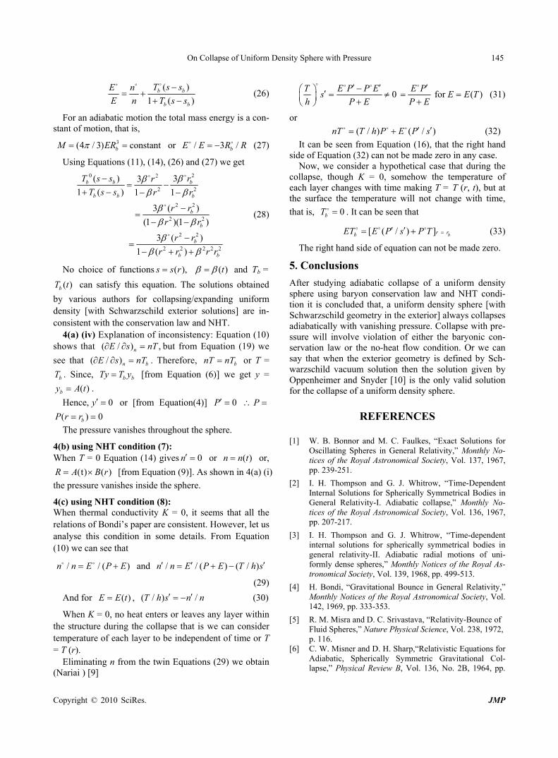
On Collapse of Uniform Density Sphere with Pressure
Copyright © 2010 SciRes. JMP
145
( )
1 ( )b b
b b
T s sE n
E n T s s
(26)
For an adiabatic motion the total mass energy is a con-stant of motion, that is,
3(4 / 3) constantbM ER or / 3 /bE E R R (27)
Using Equations (11), (14), (26) and (27) we get 0 22
2 2
2 2
2 2
2 2
2 2 2 2 2
( ) 33
1 ( ) 1 1
3 ( )
(1 )(1 )
3 ( )
1 ( )
b b b
b b b
b
b
b
b b
T s s rr
T s s r r
r r
r r
r r
r r r r
(28)
No choice of functions ( ),s s r ( )t and Tb =
( )bT t can satisfy this equation. The solutions obtained
by various authors for collapsing/expanding uniform density [with Schwarzschild exterior solutions] are in-consistent with the conservation law and NHT.
4(a) (iv) Explanation of inconsistency: Equation (10) shows that ( / ) ,nE s nT but from Equation (19) we
see that ( / )n bE s nT . Therefore, bnT nT or T =
bT . Since, b bTy T y [from Equation (6)] we get y =
( )by A t .
Hence, 0y or [from Equation(4)] 0P P
( ) 0bP r r
The pressure vanishes throughout the sphere.
4(b) using NHT condition (7): When T = 0 Equation (14) gives 0n or ( )n n t or,
(t) ( )R A B r [from Equation (9)]. As shown in 4(a) (i)
the pressure vanishes inside the sphere.
4(c) using NHT condition (8): When thermal conductivity K = 0, it seems that all the relations of Bondi’s paper are consistent. However, let us analyse this condition in some details. From Equation (10) we can see that
/ / ( )n n E P E and / / ( ) ( / )n n E P E T h s
(29)
And for ( )E E t , ( / ) /T h s n n (30)
When K = 0, no heat enters or leaves any layer within the structure during the collapse that is we can consider temperature of each layer to be independent of time or T = T (r).
Eliminating n from the twin Equations (29) we obtain (Nariai ) [9]
0T E P P E
sh P E
for ( )E P
E E TP E
(31)
or
( / ) ( / )nT T h P E P s (32)
It can be seen from Equation (16), that the right hand side of Equation (32) can not be made zero in any case.
Now, we consider a hypothetical case that during the collapse, though K = 0, somehow the temperature of each layer changes with time making T = T (r, t), but at the surface the temperature will not change with time,
that is, 0bT . It can be seen that
[ ( / ) ] br rbET E P s P T (33)
The right hand side of equation can not be made zero.
5. Conclusions
After studying adiabatic collapse of a uniform density sphere using baryon conservation law and NHT condi-tion it is concluded that, a uniform density sphere [with Schwarzschild geometry in the exterior] always collapses adiabatically with vanishing pressure. Collapse with pre- ssure will involve violation of either the baryonic con-servation law or the no-heat flow condition. Or we can say that when the exterior geometry is defined by Sch- warzschild vacuum solution then the solution given by Oppenheimer and Snyder [10] is the only valid solution for the collapse of a uniform density sphere.
REFERENCES
[1] W. B. Bonnor and M. C. Faulkes, “Exact Solutions for Oscillating Spheres in General Relativity,” Monthly No-tices of the Royal Astronomical Society, Vol. 137, 1967, pp. 239-251.
[2] I. H. Thompson and G. J. Whitrow, “Time-Dependent Internal Solutions for Spherically Symmetrical Bodies in General Relativity-I. Adiabatic collapse,” Monthly No-tices of the Royal Astronomical Society, Vol. 136, 1967, pp. 207-217.
[3] I. H. Thompson and G. J. Whitrow, “Time-dependent internal solutions for spherically symmetrical bodies in general relativity-II. Adiabatic radial motions of uni-formly dense spheres,” Monthly Notices of the Royal As-tronomical Society, Vol. 139, 1968, pp. 499-513.
[4] H. Bondi, “Gravitational Bounce in General Relativity,” Monthly Notices of the Royal Astronomical Society, Vol. 142, 1969, pp. 333-353.
[5] R. M. Misra and D. C. Srivastava, “Relativity-Bounce of Fluid Spheres,” Nature Physical Science, Vol. 238, 1972, p. 116.
[6] C. W. Misner and D. H. Sharp,“Relativistic Equations for Adiabatic, Spherically Symmetric Gravitational Col-lapse,” Physical Review B, Vol. 136, No. 2B, 1964, pp.
On Collapse of Uniform Density Sphere with Pressure
Copyright © 2010 SciRes. JMP
146
B571-576.
[7] M. Demianski, “Relativistic Astrophysics,” Pergamon Press, New York, 1985.
[8] D. Kramer, “Spherically Symmetric Radiating Solution with Heat Flow in General Relativity,” Journal of Mathematical Physics, Vol. 33, No. 4, 1992, pp. 1458- 1462.
[9] H. Nariai, “A Simple Model for Gravitational Collapse with Pressure Gradient,” Progress of Theoretical physics, Vol. 38, No. 1, 1967, pp. 92-106.
[10] J. R. Oppenheimer and H. Snyder, “On Continued Gravi-tational Contraction,” Physical Review, Vol. 56, No. 5, 1939, pp. 455-459.

Journal of Modern Physics, 2011, 2, 1156-1160 doi:10.4236/jmp.2011.210143 Published Online October 2011 (http://www.SciRP.org/journal/jmp)
Copyright © 2011 SciRes. JMP
Well Behaved Class of Charge Analogue of Durgapal’s Relativistic Exact Solution
Pratibha Fuloria1, B. C. Tewari2, B. C. Joshi3 1Department or Physics, Kumaun University, S.S.J.Campus, Almora, India
2Department of Mathematics, Kumaun University, S.S.J.Campus, Almora, India 3Department or Physics, Kumaun University, S.S.J.Campus, Almora, India
E-mail: [email protected], [email protected] Received July 12, 2011; revised August 26, 2011; accepted September 6, 2011
Abstract We obtain a new class of charged super-dense star models after prescribing particular Forms of the metric potential and electric intensity. The metric describing the superdense stars joins smoothly with the Reiss-ner-Nordstrom metric at the pressure free boundary. The interior of the stars possess their energy density, pressure, pressure density ratio and velocity of sound to be monotonically decreasing towards the pressure free interface. In view of the surface density 14 32 10 g cmb , the heaviest star occupies a mass 5.523 Mwith its radius 13.98 km. In absence of the charge we are left behind with the regular and well behaved fifth model of Durgapal [1]. Keywords: Charged Fluids, Reissener-Nordstom Metric, General Relativity
1. Introduction Exact interior solutions of the Einstein-Maxwell field equations joining smoothly to the Nordstrom solution at the pressure free interface are gathering big applause due to some of the following reasons: 1) Gravitational col-lapse of a charged fluid sphere to a point singularity may be avoided. 2) Solutions of Einstein-Maxwell equations are useful in the study of cosmic sensership. 3) Charged- dust models and electromagnetic mass models are ex-pected to provide some clue about structure of an elec-tron . In the present paper our aim is to obtain a class of regular and well behaved charged fluid models whose neutral analogues are also regular and well behaved. Here we consider a spherically symmetric metric which shares its metric potential with one of the Durgapal’s interior metric [1].
On account of the nonlinearity of Einstein-Maxwell field equations, not many realistic well behaved, analytic solutions are known for the description of relativistic charge fluid spheres. For well behaved model of relativ-istic star with charged and perfect fluid matter, following conditions should be satisfied (Pant et al. [2]):
1) The solution should be free from physical and geo-metrical singularities i.e. finite and positive values of central pressure, central density and non zero positive
values of e and e . 2) The solution should have positive and monotoni-
cally decreasing expressions for pressure and density ( andp ) with the increase of r. The solution should have positive value of ratio of pressure-density and less than 1(weak energy condition) and less than 1/3(strong energy condition) throughout within the star.
3) The solution should have positive and monotoni- cally decreasing expression for fluid parameter 2P c with the increase of r.
4) The solution should have positive and monotoni-
cally decreasing expression for velocity of sound d
( )d
p
with the increase of r and causality condition should be
obeyed at the centre, i.e., 2
d1
d
p
c ..
5) The red shift Z should be positive, finite and mono- tonically decreasing in nature with the increase of r.
Electric intensity E is positive and monotonically in-creasing from centre to boundary and at the centre the Electric intensity is zero.
Under these well behaved conditions, one has to as-sume the gravitational potential and electric field inten-sity in such a way that the field equation can be inte-grated and solution should be well behaved. Keeping in

P. FULORIA ET AL.
1157
view of this aspect ,several authors obtained the para-metric class of exact solutions Pant et al. [3,4], Gupta- Maurya [5-7], Pant [8,9], N. Bijalwan [10] etc. These coupled solutions are well behaved with some positive values of charge parameter K and completely describe interior of the super-dense astrophysical object with charge matter. Further, The mass of the such modeled super dense object can be maximized by assuming sur-face density is 14 32 10 g cmb . In the present paper we have obtained yet another new parametric class of well behaved exact solutions of Einstein-Maxwell field equations, which is compatible within the range of Neu-tron star and quark star. 2. Einstein’s–Maxwell Equation for Charged
Fluid Distribution Let us consider a spherical symmetric metric in curvature coordinates
2 2 2 2 2 2 2d d d sin d 2ds e r r r e t (1)
where the functions r and satisfy the Ein-stein-Maxwell equations
r
4
24
8 1
28
1 1
4 4
i i ij j j
i j ij
im i mnjm j mn
GT R R
cG
c p v v pc
F F F F
(2)
where , p, , Fij denote energy density, fluid pres-sure, velocity vector and skew-symmetric electromag-netic field tensor respectively.
iv
In view of the metric (1), the field equation (2) gives Dionysiou [11]
2
2 4
1 8e G qe p
r r c
4r (3)
2
4
8
2 4 4 2
G qe p
r c r
2
4 (4)
2
2 2
1 8e G qe
r r c
4r (5)
where prime ( ' ) denotes the differentiation with respect to r and represents the total charge contained with in the sphere of radius r.
q r
By using the transformation
5 211 , ande B x x c r e Z (6)
where B being the positive constants. Now putting (6)
into (3)-(5), we have
2
12
1
110 1 8
1
Z c q4
Z GP
x x cx c
(7)
21
21
1 d 1 82
d
Z c q4
Z G
x X cx c
(8)
and Z satisfying the equation
22
12 1 1d 14 2 1
d 1 1 6 1 6
q c x xZ x xZ
x x x x x x x
(9)
where 21 ,x c r e Z .
3. New Class of Solutions In order to solve the differential equation (9) let us con-sider the electric intensity E of the following form
22 2
1 32
1
1 1 62
c qE Kxx x
c x (10)
where K is a positive constant. The electric density is so assumed that the model is physically significant and well behaved, i.e., E remains regular and positive throughout the sphere.
In view of (10) differential equation (9) yields the fol-lowing solution
3
1/3
2
3
3
1
3
1
6 1 6
309 54 811
1121
11 6
x xKe
x
x x x
x
Axx
x
(11)
where A is an arbitrary constant of integration. 4. Properties of the New Class of Solutions Using (11), into (7) and (8), we get the following expres-sions for pressure and energy density
41
2 3
4 1
3
2
1 8
475 4125 1050 200 1 111
1121 1 6
1 1 15 29
16 1 63
Gp
c c
x x x A x
x x
x x xK
x
(12)
Copyright © 2011 SciRes. JMP

P. FULORIA ET AL.
Copyright © 2011 SciRes. JMP
1158
41
2 3
2
4
3
2 3
4
3
1 8
1935 15 450 1201
1 4 112
3 11 22
1 6
1 3 29 109 158
6 1 6
G
c c
x x x
x
x xA
x
x x x xk
x
(13)
41 0
1 8 d 6025 75
d 112
G p KA
c xc
3 (18)
41 0
1 8 d 7725 425
d 112 3
G KA
c xc
(19)
The velocity of sound is given by the following ex-pression (20)-(21)
20
7841205 1121 d 15
448d 1545 56015
x
A Kp
c A K
(21)
The expression for gravitational red-shift (z) is given by
041
1 8 475
112 6
Gp A
c c
K (14)
5
211
xz
B
(22)
041
1 8 19353
112 2
G KA
c c
(15)
The central value of gravitational red shift to be non zero positive finite, we have Differenting (12) and (13) w.r.t. x, we get:
41
2 3
5
2 2
45
3
1 8 d
d
25 241 411 60 8
112 1
5 1 3 44 14 152 527 464
46 1 61 1 6
3
G p
c xc
x x x
x
3A x x K x x x
xx x
1 B 0 (22a)
Differenting (22) w.r.t. x, we get,
0
d 50
d 2x
z
x B
(22b)
the expression of right hand side of (22b) is negative, thus the gravitational red-shift is maximum at the center and monotonically decreasing. (16)
41
2 35
2 37
53
2 37
3
1 8 d
d
15515 57 36 8
112 1
55 39 66 88
1 1 6
8 212 1353 3302 2528
6(1 6 )
G
c xc
x x xx
Ax x x
x x
K
5. Boundary Conditions
4x x x
x
x
The solutions so obtained are to be matched over the boundary with Reissner-Nordstrom metric:
122 2
2
22 2 2 2
2
2d 1 d
2d sin d 1 d
GM es r
r r
GM er t
r r
2
(23)
which requires the continuity of ,e e and q across the boundary r = rb (17)
2 d
d
pv
4 452 3 2 2 33 3
7 7252 3 2 3 2 3 43 3
1125 241 411 60 8 112 1 3 44 1 6 14 152 527 464 1 6 11 d 30
112d 3 515 57 36 8 112 5 39 66 88 1 6 (8 212 1353 3302 2528 ) 1 6 130
x x x A x x x K x x x x xp
c x x x A x x x x K x x x x x x
(20)
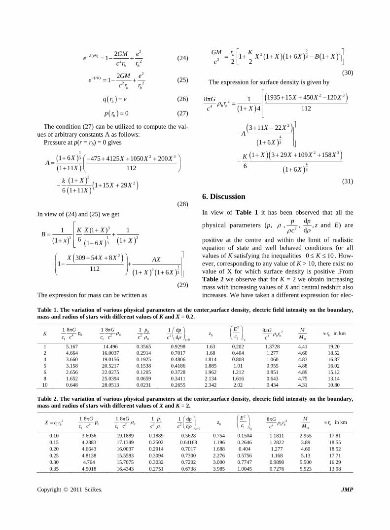
2( )
2
21rb
b b
GM ee
c r r
2 (24)
2( )
2
21rb
b b
GM ee
c r r
2 (25)
bq r e (26)
0bp r (27)
The condition (27) can be utilized to compute the val-ues of arbitrary constants A as follows:
Pressure at p(r = rb) = 0 gives
12 33
5
2
1 6 475 4125 1050 200
1 11 112
11 15 29
6 1 11
X X X XA
X
XkX X
X
(28)
In view of (24) and (25) we get
3
5 1 3
3
2
13
3
1 (1 ) 1
61 11 6
309 54 81
112 1 1 6
K X XB
x XX
X X X AX
X X
(29)
The expression for mass can be written as
2
52 32
1 1 1 6 12 2brGM K
X X X B Xc
(30)
The expression for surface density is given by
2 3
24
2
4
3
2 3
4
3
1935 15 450 1208 1
1 4 112
3 11 22
1 6
1 3 29 109 158
6 1 6
b b
X X XGr
Xc
X XA
X
X X X XK
X
(31) 6. Discussion In view of Table 1 it has been observed that all the
physical parameters (p, ,2
,p
cd
,d
pz
and E) are
positive at the centre and within the limit of realistic equation of state and well behaved conditions for all values of K satisfying the inequalities . How-ever, corresponding to any value of K > 10, there exist no value of X for which surface density is positive .From Table 2 we observe that for K = 2 we obtain increasing mass with increasing values of X and central redshift also increases. We have taken a different expression for elec-
0 K 10
Table 1. The variation of various physical parameters at the center,surface density, electric field intensity on the boundary, mass and radius of stars with different values of K and X = 0.2.
K 041
1 8 Gp
c c
02
1
1 8 G
c c
02
0
1 p
c
20
1 d
d x
p
c
0z 2
1br
E
c
22
8b b
Gr
c
M
M
br in km
1 5.167 14.496 0.3565 0.9298 1.63 0.202 1.3728 4.41 19.20 2 4.664 16.0037 0.2914 0.7017 1.68 0.404 1.277 4.60 18.52 4 3.660 19.0156 0.1925 0.4806 1.814 0.808 1.060 4.83 16.87 5 3.158 20.5217 0.1538 0.4186 1.885 1.01 0.955 4.88 16.02 6 2.656 22.0275 0.1205 0.3728 1.962 1.212 0.851 4.89 15.12 8 1.652 25.0394 0.0659 0.3411 2.134 1.616 0.643 4.75 13.14
10 0.648 28.0513 0.0231 0.2655 2.342 2.02 0.434 4.31 10.80 Table 2. The variation of various physical parameters at the center,surface density, electric field intensity on the boundary, mass and radius of stars with different values of X and K = 2.
21 bX c r 04
1
1 8 Gp
c c
02
1
1 8 G
c c
02
0
1 p
c
20
1 d
d x
p
c
0z 2
1br
E
c
22
8b b
Gr
c
M
M
br in km
0.10 3.6036 19.1889 0.1889 0.5628 0.754 0.1504 1.1811 2.955 17.81 0.15 4.2883 17.1349 0.2502 0.64168 1.196 0.2646 1.2822 3.89 18.55 0.20 4.6643 16.0037 0.2914 0.7017 1.688 0.404 1.277 4.60 18.52 0.25 4.8138 15.5583 0.3094 0.7300 2.276 0.5756 1.168 5.13 17.71 0.30 4.764 15.7075 0.3032 0.7202 3.000 0.7747 0.9890 5.500 16.29 0.35 4.5018 16.4343 0.2751 0.6738 3.985 1.0045 0.7276 5.523 13.98
Copyright © 2011 SciRes. JMP

1160 P. FULORIA ET AL.
tric intensity as compared to that of Gupta and Mau-raya’s solution [5]. Our solution satisfies all the neces-sary physical conditions giving us a possibitity for dif-ferent charge variations within the fluid sphere. Owing to the various conditions that we obtain here we arrive at the conclusion that under well behaved conditions this class of solutions gives us the mass of super dense object within the range of neutron star and quark star.
We now present here a model of super dense star based on the particular solution discussed above corre-sponding to K = 0.35 with , by assuming sur-face density;
0.2X 14 32 10 g cmb .The resulting well
behaved model has the heaviest star occupying a mass 5.523 M with its radius 13.98 km. In absence of the charge we are left behind with the regular and well be-haved fifth model of Durgapal [1]. 7. References [1] M. C. Durgapal, “A Class of New Exact Solutions in
General Relativity,” Journal of Physics A: Mathematical and General, Vol. 15, August 1982, pp. 2637-2644.
[2] N. Pant, “Some New Exact Solutions with Finite Central Parameters and Uniform Radial Motion of Sound,” As-trophysics and Space Science, Vol. 331, No. 2, 2011, pp. 633-644. doi:10.1007/s10509-010-0453-4
[3] N. Pant, et al., “Well Behaved Class of Charge Analogue of Heintzmann’s Relativistic Exact Solution,” Astrophys-ics and Space Science, Vol. 332, No. 2, 2011, pp. 473- 479. doi:10.1007/s10509-010-0509-5
[4] N. Pant, et al., “Variety of Well Behaved Parametric Classes of Relativistic Charged Fluid Spheres in General Relativity,” Astrophysics and Space Science, Vol. 333, No. 1, 2011, pp. 161-168.
[5] Y. K. Gupta and S. K. Maurya, “A Class of Regular and Well Behaved Relativistic Super Dense Star Models,” Astrophysics and Space Science, Vol. 334, No. 1, 2011, pp. 155-162. doi:10.1007/s10509-010-0503-y
[6] S. K. Maurya and Y. K. Gupta, “A Family of Well Be-haved Charge Analogue of a Well Behaved Neutral Solu-tion in Genetral Relativity,” Astrophysics and Space Sci-ence, Vol. 332, No. 2, 2011, pp. 481-490. doi:10.1007/s10509-010-0541-5
[7] S. K. Maurya and Y. K. Gupta, “Charged Analogue of Vlasenko-Pronin Super Dense Star in General Relativ-ity,” Astrophysics and Space Science, Vol. 333, No. 1, 2011, pp. 149-160. doi:10.1007/s10509-011-0616-y
[8] N. Pant, “Well Behaved Parametric Class of Relativistic in Charged Fluid Ball General Relativity,” Astrophysics and Space Science, Vol. 332, No.2, 2011, pp.403-408. doi:10.1007/s10509-010-0521-9
[9] N. Pant, “New Class of Well Behaved Exact Solutions of Relativistic Charged White-Dwarf Star with Perfect Fluid,” Astrophysics and Space Science, Vol. 334, No. 2, 2011, pp. 267-271. doi:10.1007/s10509-011-0720-z
[10] N. Bijalwan, “Static Electrically Charged Fluids in Terms Pressure: General Relativity,” Astrophysics and Space Science, Vol. 334, No. 1, 2011, pp.139-143. doi:10.1007/s10509-011-0691-0
[11] D. D. Dionysiou, “Equilibrium of a Static Charged Per-fect Fluid Sphere,” Astrophysics and Space Science, Vol. 85, No. 1-2, 1982, pp. 331-343. doi:10.1007/BF00653455
Copyright © 2011 SciRes. JMP

Journal of Modern Physics, 2011, 2, 1538-1543 doi:10.4236/jmp.2011.212186 Published Online December 2011 (http://www.SciRP.org/journal/jmp)
Copyright © 2011 SciRes. JMP
Well Behaved Parametric Class of Exact Solutions of Einstein-Maxwell Field Equations in General Relativity
Neeraj Pant1, B. C. Tewari2, Pratibha Fuloria3 1Department of Mathematics, National Defence Academy Khadakwasla, Pune, India
2Department of Mathematics, Kumaun University, S.S.J. Campus, Almora, India 3Department of Physics Kumaun University, S.S.J. Campus, Almora, India
E-mail: {neeraj.pant, p.fuloria}@yahoo.com Received September 15, 2011; revised October 27, 2011; accepted November 22, 2011
Abstract We present a new well behaved class of exact solutions of Einstein-Maxwell field equations. This solution describes charge fluid balls with positively finite central pressure, positively finite central density; their ratio is less than one and causality condition is obeyed at the centre. The gravitational red shift is positive throughout positive within the ball. Outmarch of pressure, density, pressure-density ratio, the adiabatic speed of sound and gravitational red shift is monotonically decreasing, however, the electric intensity is monotoni-cally increasing in nature. The solution gives us wide range of parameter K (0.72 ≤ K ≤ 2.41) for which the solution is well behaved hence, suitable for modeling of super dense star. For this solution the mass of a star is maximized with all degree of suitability and by assuming the surface density ρb = 2 × 10¹⁴ g/cm3. Corre-sponding to K = 0.72 with X = 0.15, the resulting well behaved model has the mass M = 1.94 MΘ with radius rb 15.2 km and for K = 2.41 with X = 0.15, the resulting well behaved model has the mass M = 2.26 MΘ with radius rb 14.65 km. Keywords: Charge Fluid, Reissner-Nordstrom, General Relativity, Exact Solution
1. Introduction Ever since the formulation of Einstein-Maxwell field equations, the relativists have been proposing different models of immense gravity astrophysical objects by con-sidering the distinct nature of matter or radiation (en-ergy-momentum tensor) present in them. Such models successfully explain the characteristics of massive ob-jects like quasar, neutron star, pulsar, quark star, black- hole or other super-dense object. These stars are speci-fied in terms of their masses as white dwarfs (Mass < 1.44 solar mass), Quark star (2 solar mass - 3 solar mass) and Neutron star (1.35 solar mass - 2.1 solar mass).
It is well known that the Reissener-Nordstrom solution for the external field of a ball of charged mass has two distinct singularities at finite radial positions other than at the centre. Thus the solution describes a bridge (worm hole) between two asymptotically flat spaces and an electric flux flowing across the bridge. Graves and Bill [1] pointed out that the region of minimum radius or the throat of worm hole pulsates periodically between these two surfaces due to Maxwell pressure of the electric field.
Consequently, unlike Schwarzschild’s exterior solution of chargeless matter,in Reissener-Nordstrom solution has no surface which can catastrophically hit the geometric singularity at r = 0.All these aspects show that the pres- ence of some charge in a spherical material distribution provides an additional resistance against the gravita- tional contraction by mean of electric repulsion and hence ,the catastrophic collapse of the entire mass to a point singularity can be avoided.
The above result has been supported by a physically reasonable charge spherical model of Bonnor [2], that a dust distribution of arbitrarily large mass and small ra-dius can remain in equilibrium against the pull of gravity by a repulsive force produced by a small amount of charge. Thus it is desirable to study the implications of Einstein-Maxwell field equations with reference to the general relativistic prediction of gravitational collapse. For this purpose charged fluid ball models are required. The external field of such ball is to be matched with Reissener-Nordstrom solution.
For obtaining significant charged fluid ball models of Einstein-Maxwell field equations, the Astrophysicists
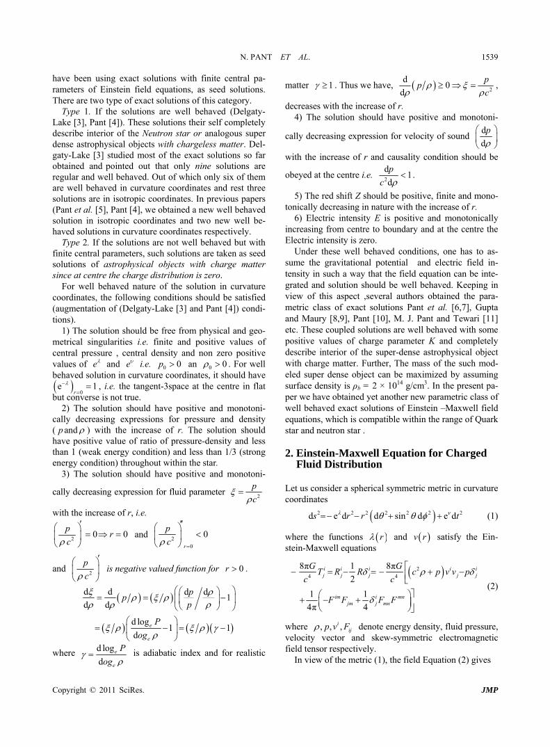
N. PANT ET AL. 1539 have been using exact solutions with finite central pa-rameters of Einstein field equations, as seed solutions. There are two type of exact solutions of this category.
Type 1. If the solutions are well behaved (Delgaty- Lake [3], Pant [4]). These solutions their self completely describe interior of the Neutron star or analogous super dense astrophysical objects with chargeless matter. Del- gaty-Lake [3] studied most of the exact solutions so far obtained and pointed out that only nine solutions are regular and well behaved. Out of which only six of them are well behaved in curvature coordinates and rest three solutions are in isotropic coordinates. In previous papers (Pant et al. [5], Pant [4], we obtained a new well behaved solution in isotropic coordinates and two new well be-haved solutions in curvature coordinates respectively.
Type 2. If the solutions are not well behaved but with finite central parameters, such solutions are taken as seed solutions of astrophysical objects with charge matter since at centre the charge distribution is zero.
For well behaved nature of the solution in curvature coordinates, the following conditions should be satisfied (augmentation of (Delgaty-Lake [3] and Pant [4]) condi-tions).
1) The solution should be free from physical and geo-metrical singularities i.e. finite and positive values of central pressure , central density and non zero positive values of e and e i.e. 0 an 00p 0 . For well behaved solution in curvature coordinates, it should have
0r, i.e. the tangent-3space at the centre in flat
but converse is not true. e 1
2) The solution should have positive and monotoni-cally decreasing expressions for pressure and density ( and p ) with the increase of r. The solution should have positive value of ratio of pressure-density and less than 1 (weak energy condition) and less than 1/3 (strong energy condition) throughout within the star.
3) The solution should have positive and monotoni-
cally decreasing expression for fluid parameter 2
p
c
with the increase of r, i.e.
20
pr
c
0 and
20
0r
p
c
and 2
p
c
0r is negative valued function for .
d d d d1
d d
d log 1 1
de
e
pp
p
P
og
where d log
de
e
P
og
is adiabatic index and for realistic
matter 1 . Thus we have, 2
d0
d
pp
c
,
decreases with the increase of r. 4) The solution should have positive and monotoni-
cally decreasing expression for velocity of sound d
d
p
with the increase of r and causality condition should be
obeyed at the centre i.e. 2
d1
d
p
c .
5) The red shift Z should be positive, finite and mono-tonically decreasing in nature with the increase of r.
6) Electric intensity E is positive and monotonically increasing from centre to boundary and at the centre the Electric intensity is zero.
Under these well behaved conditions, one has to as-sume the gravitational potential and electric field in-tensity in such a way that the field equation can be inte-grated and solution should be well behaved. Keeping in view of this aspect ,several authors obtained the para-metric class of exact solutions Pant et al. [6,7], Gupta and Maury [8,9], Pant [10], M. J. Pant and Tewari [11] etc. These coupled solutions are well behaved with some positive values of charge parameter K and completely describe interior of the super-dense astrophysical object with charge matter. Further, The mass of the such mod-eled super dense object can be maximized by assuming surface density is ρb = 2 × 10¹⁴ g/cm3. In the present pa-per we have obtained yet another new parametric class of well behaved exact solutions of Einstein –Maxwell field equations, which is compatible within the range of Quark star and neutron star . 2. Einstein-Maxwell Equation for Charged
Fluid Distribution Let us consider a spherical symmetric metric in curvature coordinates
2 2 2 2 2 2d e d d sin d e d 2s r r t (1)
where the functions r and satisfy the Ein-stein-Maxwell equations
v r
24 4
8π 1 8π
2
1 1
4π 4
i i i i ij j j j j
im i mnjm j mn
G GT R R c p v v p
c c
F F F F
(2)
where denote energy density, fluid pressure, velocity vector and skew-symmetric electromagnetic field tensor respectively.
, , ,iijp v F
In view of the metric (1), the field Equation (2) gives
Copyright © 2011 SciRes. JMP

N. PANT ET AL.
Copyright © 2011 SciRes. JMP
1540
2
2 4
1 e 8πe
vp
r r c
Our task is to explore the solutions of Equation (9) and obtain the fluid parameters and p from Equation (7) and Equation (8).
4
G q
r (3)
2 2
4
8πe
2 4 4 2
v v v v G qp
r c r
4
(4) 3. New Class of Solutions
2
2 2
1 e 8πe
G q
r r c
In order to solve the differential Equation (9), In this paper we consider the electric intensity E of the follow-ing form
4r
(5)
where, prime (/)denotes the differentiation with respect to r and q(r) represents the total charge contained within the sphere of radius r.
22 1
1 32
1
1 3 12
c qE K x xc x
x (10)
Now let us set where K is a positive constant. The electric intensity is so assumed that the model is physically significant and well behaved i.e. E remains regular and positive throughout the sphere. In addition, E vanishes at the centre of the star.
2211ve B c r (6)
which is the same as that of the metric obtained by Adler [12].
Putting (6) into (3) - (5) , we have In view of Equation (10) differential Equation (9) yields the following solution 2
12 4
1
14 π
1
Z c q 1 8Z Gp
x x cx c
(7)
3
2
3 3
(1 )e 1
3 1 3 1 3
2
K x x AxZ
x x (11a)
21
2 21
1 d 1 8π2
d
Z c qZ G
x x cx c
(8)
where A is an arbitrary constant of integration.
and Z satisfying the equation 21ve B x (11b)
21
1 2d 11
d 1 3 1 3
x c qZ xZ
x x x x x x
(9) Using (11a), (11b) into Equations (7) and (8), we get the following expressions for pressure and energy den-sity where 2
1 , ex c r Z .
2
4 21 3 3
19 15 2 1 1 51 8π 4
6 11 3 1 1 3
2
x x x A xG Kp
c xc x x x (12)
3 2
5
2 5
1 3 3
1 73 92 37 6 3 51 8π
6 1 3 1 3
x x x x A xG K
c c x x (13)
4. Properties of the New Class of Solutions
For 0 andp 0 must be positive and 0
0
1p
, we
The central values of pressure and density are given by have
041
1 8π4
3
G Kp A
c c (14)
4 13 3
K KA , and (16) 0, 0K A
021
1 8π3
GK A
c c (15) Differentiating (12) and (13) w. r. t. x, we get;
3 2 2
4 521 3 3
63 123 65 13 1 51 8π d 42
d 6 11 3 1 1 3
x x x xG p KA
c xc 5 2xx x x
(17)
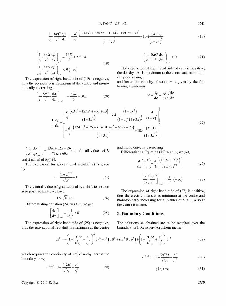
N. PANT ET AL. 1541
4 3 2
2 81 3 3
1241 2602 1914 602 73 11 8π d. 1
d 6 1 3(1 3 )
x x x x xG KA
c xc 80
xx
(18)
41 0
41 0
1 8π d 132 4
d 6
1 8π d0
d
x
x
G p KA
c xc
G pve
c xc
(19)
The expression of right hand side of (19) is negative, thus the pressure p is maximum at the centre and mono-tonically decreasing.
21 0
1 8π d 7310
d 6
x
G KA
c xc (20)
21 0
1 8π d0
d
x
G
c xc (21)
The expression of right hand side of (20) is negative, the density is maximum at the centre and monotoni-cally decreasing. and hence the velocity of sound v is given by the fol-lowing expression
2 d d d
d dd
p p pv
x x
3 2 2
5 52
3 3
24 3 2
8 8
3 3
63 123 65 13 1 5 42
6 11 3 1 1 31 d
d 1241 2602 1914 602 73 110
6 1 3 1 3
x x x xKA
xx x xp
c x x x x xKA
x x
2
(22)
20
1 d 13 12 241
d 73 60r
p K A
K Ac
, for all values of K
and A satisfied by(16). The expression for gravitational red-shift(z) is given
by
11
1x
zB
(23)
The central value of gravitational red shift to be non zero positive finite, we have
1 B 0 (24)
Differentiating equation (24) w.r.t. x, we get,
0
d 10
d x
z
x B
(25)
The expression of right hand side of (25) is negative, thus the gravitational red-shift is maximum at the centre
and monotonically decreasing. Differentiating Equation (10) w.r.t. x, we get,
22
2 31
1 6 7d
d 2 1 3
x xE K
x c x
(26)
2
1 0
d ve
d 2x
E K
x c
(27)
The expression of right hand side of (27) is positive, thus the electric intensity is minimum at the centre and monotonically increasing for all values of K > 0. Also at the centre it is zero. 5. Boundary Conditions The solutions so obtained are to be matched over the boundary with Reissner-Nordstrom metric.;
12 2
2 2 2 2 2 22 2 2 2
2 2d 1 d d sin d 1
b b b b
GM e GM e 2ds r r tc r r c r r
(28)
which requires the continuity of across the boundary .
, ande e q
br r2
( )2
21br
b b
GM ee
c r r
2( )
2
21br
b b
GM ee
c r r
2 (30)
2 (29) bq r e (31)
Copyright © 2011 SciRes. JMP

N. PANT ET AL. 1542
0bp r (32)
The condition (30) can be utilized to compute the val-ues of arbitrary constants A as follows:
On setting br r
21 ,bx X c r ( being the radius of
the charged sphere) br
Pressure at gives ( ) 0br rp
2 2 2 31 19 15 2 1 34
6 1 5 1 5
X X X XKA
X X (33)
The expression for mass can be written as
22
1 7 22 1 3 2 3 6brGM X K
X X X AXc
(34)
In view of (29) and (30) we get,
3
2 3 2 3
2
11
3 1 3 1 3
1
XKX XA
X XB
X
Centre red shift is given by 1/2
0 1z B (35)
In view of and TableI and Table-II We observe that pressure, density, pressure-density ratio, square of adia- batic sound speed and gravitational red shift decrease monotonically with the increase of radial coordinate
however, the charge distribution is increasing in nature. 6. Discussion In view of and Tables 1 and 2, it has been observed
, 2
,p
c ,
dpz
d that all the physical parameters (p,
and E) are positive at the centre and within the limit of realistic equation of state and well behaved conditions for all values of K satisfying the inequalities 0.72 ≤ K ≤ 2.41. However, corresponding to any value of K < 0.72, there exist no value of X for which the nature of adia- batic sound speed is monotonically decreasing from centre to pressure free interface and for K > 2.41 , the pressure is negative some where within the ball for all values of X. It has been observed that under well be- haved conditions this class of solutions gives us the mass of super dense object within the range of quark star and neutron star.
We now present here two models of super dense star based on the particular solution discussed above by as-suming surface density; ρb = 2 × 10¹⁴ g/cm3. Corre-sponding to K = 0.72 with X = 0.15, the resulting well behaved model has the mass M = 1.94 MΘ
.with radius rb 15.2 km and for K = 2.41 with X = 0.15, the resulting well behaved model has the mass M = 2.26 MΘwith ra-dius rb 14.65 km.
Table 1. The march of pressure, density, pressure-density ratio, square of adiabatic sound speed, gravitational red shift and electric field intensity within the ball corresponding to K = 0.72 with X = 0.15.
br r 2
4
8πb
Gp r
c 2
2
8πb
Gr
c 2
p
c
2
1 d
d
p
c
z 2
bE r
0 0.133143 1.400572 0.095063 0.216271 0.426164 0
0.1 0.131095 1.392716 0.094129 0.216101 0.424028 0.00008
0.2 0.125065 1.369595 0.091315 0.215525 0.417658 0.000332
0.3 0.115385 1.332484 0.086594 0.214356 0.407167 0.000769
0.4 0.10257 1.283297 0.079927 0.212291 0.392738 0.001422
0.5 0.087277 1.224339 0.071285 0.208939 0.374616 0.002334
0.6 0.070247 1.158033 0.060661 0.203855 0.353097 0.003562
0.7 0.052258 1.086683 0.048089 0.196582 0.328518 0.005177
0.8 0.034079 1.01231 0.033664 0.186713 0.301245 0.007265
0.9 0.016437 0.936551 0.017551 0.173954 0.271658 0.00993
1.0 0 0.860627 0 0.158177 0.240143 0.013294
Copyright © 2011 SciRes. JMP
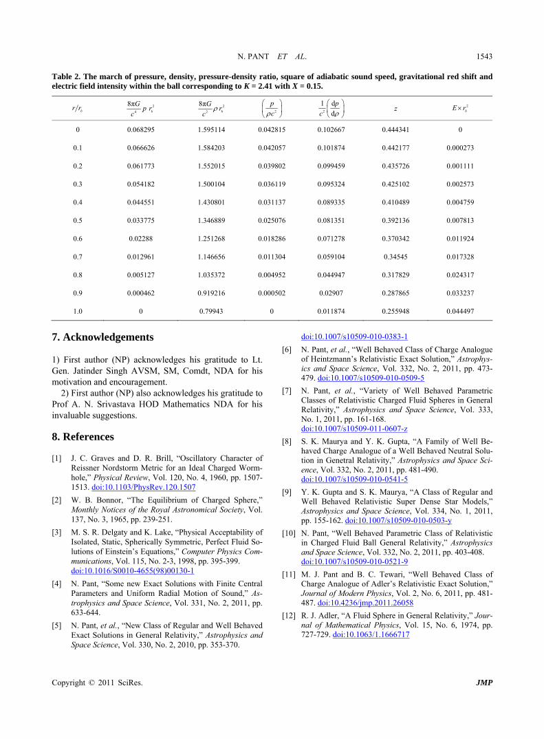
N. PANT ET AL. 1543 Table 2. The march of pressure, density, pressure-density ratio, square of adiabatic sound speed, gravitational red shift and electric field intensity within the ball corresponding to K = 2.41 with X = 0.15.
br r 2
4
8πb
Gp r
c 2
2
8πb
Gr
c 2
p
c
2
1 d
d
p
c
z 2
bE r
0 0.068295 1.595114 0.042815 0.102667 0.444341 0
0.1 0.066626 1.584203 0.042057 0.101874 0.442177 0.000273
0.2 0.061773 1.552015 0.039802 0.099459 0.435726 0.001111
0.3 0.054182 1.500104 0.036119 0.095324 0.425102 0.002573
0.4 0.044551 1.430801 0.031137 0.089335 0.410489 0.004759
0.5 0.033775 1.346889 0.025076 0.081351 0.392136 0.007813
0.6 0.02288 1.251268 0.018286 0.071278 0.370342 0.011924
0.7 0.012961 1.146656 0.011304 0.059104 0.34545 0.017328
0.8 0.005127 1.035372 0.004952 0.044947 0.317829 0.024317
0.9 0.000462 0.919216 0.000502 0.02907 0.287865 0.033237
1.0 0 0.79943 0 0.011874 0.255948 0.044497
7. Acknowledgements 1) First author (NP) acknowledges his gratitude to Lt. Gen. Jatinder Singh AVSM, SM, Comdt, NDA for his motivation and encouragement.
2) First author (NP) also acknowledges his gratitude to Prof A. N. Srivastava HOD Mathematics NDA for his invaluable suggestions. 8. References [1] J. C. Graves and D. R. Brill, “Oscillatory Character of
Reissner Nordstorm Metric for an Ideal Charged Worm-hole,” Physical Review, Vol. 120, No. 4, 1960, pp. 1507- 1513. doi:10.1103/PhysRev.120.1507
[2] W. B. Bonnor, “The Equilibrium of Charged Sphere,” Monthly Notices of the Royal Astronomical Society, Vol. 137, No. 3, 1965, pp. 239-251.
[3] M. S. R. Delgaty and K. Lake, “Physical Acceptability of Isolated, Static, Spherically Symmetric, Perfect Fluid So- lutions of Einstein’s Equations,” Computer Physics Com- munications, Vol. 115, No. 2-3, 1998, pp. 395-399. doi:10.1016/S0010-4655(98)00130-1
[4] N. Pant, “Some new Exact Solutions with Finite Central Parameters and Uniform Radial Motion of Sound,” As- trophysics and Space Science, Vol. 331, No. 2, 2011, pp. 633-644.
[5] N. Pant, et al., “New Class of Regular and Well Behaved Exact Solutions in General Relativity,” Astrophysics and Space Science, Vol. 330, No. 2, 2010, pp. 353-370.
doi:10.1007/s10509-010-0383-1
[6] N. Pant, et al., “Well Behaved Class of Charge Analogue of Heintzmann’s Relativistic Exact Solution,” Astrophys- ics and Space Science, Vol. 332, No. 2, 2011, pp. 473- 479. doi:10.1007/s10509-010-0509-5
[7] N. Pant, et al., “Variety of Well Behaved Parametric Classes of Relativistic Charged Fluid Spheres in General Relativity,” Astrophysics and Space Science, Vol. 333, No. 1, 2011, pp. 161-168. doi:10.1007/s10509-011-0607-z
[8] S. K. Maurya and Y. K. Gupta, “A Family of Well Be-haved Charge Analogue of a Well Behaved Neutral Solu- tion in Genetral Relativity,” Astrophysics and Space Sci- ence, Vol. 332, No. 2, 2011, pp. 481-490. doi:10.1007/s10509-010-0541-5
[9] Y. K. Gupta and S. K. Maurya, “A Class of Regular and Well Behaved Relativistic Super Dense Star Models,” Astrophysics and Space Science, Vol. 334, No. 1, 2011, pp. 155-162. doi:10.1007/s10509-010-0503-y
[10] N. Pant, “Well Behaved Parametric Class of Relativistic in Charged Fluid Ball General Relativity,” Astrophysics and Space Science, Vol. 332, No. 2, 2011, pp. 403-408. doi:10.1007/s10509-010-0521-9
[11] M. J. Pant and B. C. Tewari, “Well Behaved Class of Charge Analogue of Adler’s Relativistic Exact Solution,” Journal of Modern Physics, Vol. 2, No. 6, 2011, pp. 481- 487. doi:10.4236/jmp.2011.26058
[12] R. J. Adler, “A Fluid Sphere in General Relativity,” Jour- nal of Mathematical Physics, Vol. 15, No. 6, 1974, pp. 727-729. doi:10.1063/1.1666717
Copyright © 2011 SciRes. JMP

1 23
Astrophysics and Space ScienceAn International Journal of Astronomy,Astrophysics and Space Science ISSN 0004-640XVolume 340Number 2 Astrophys Space Sci (2012) 340:407-412DOI 10.1007/s10509-012-1068-8
A new well behaved exact solution ingeneral relativity for perfect fluid
Neeraj Pant, Pratibha Fuloria &B. C. Tewari

1 23
Your article is protected by copyright and
all rights are held exclusively by Springer
Science+Business Media B.V.. This e-offprint
is for personal use only and shall not be self-
archived in electronic repositories. If you
wish to self-archive your work, please use the
accepted author’s version for posting to your
own website or your institution’s repository.
You may further deposit the accepted author’s
version on a funder’s repository at a funder’s
request, provided it is not made publicly
available until 12 months after publication.

Astrophys Space Sci (2012) 340:407–412DOI 10.1007/s10509-012-1068-8
O R I G I NA L A RT I C L E
A new well behaved exact solution in general relativity for perfectfluid
Neeraj Pant · Pratibha Fuloria · B.C. Tewari
Received: 14 February 2012 / Accepted: 31 March 2012 / Published online: 20 April 2012© Springer Science+Business Media B.V. 2012
Abstract We present a new spherically symmetric solutionof the general relativistic field equations in isotropic coordi-nates. The solution is having positive finite central pressureand positive finite central density. The ratio of pressure anddensity is less than one and casualty condition is obeyed atthe centre. Further, the outmarch of pressure, density andpressure-density ratio, and the ratio of sound speed to lightis monotonically decreasing. The solution is well behavedfor all the values of u lying in the range 0 < u ≤ .186. Thecentral red shift and surface red shift are positive and mono-tonically decreasing. Further, we have constructed a neutronstar model with all degree of suitability and by assuming thesurface density ρb = 2×10¹⁴ g/cm3. The maximum mass ofthe Neutron star comes out to be M = 1.591 M� with radiusRb ≈ 12.685 km. The most striking feature of the solution isthat the solution not only well behaved but also having oneof the simplest expressions so far known well behaved solu-tions. Moreover, the good matching of our results for Velapulsars show the robustness of our model.
Keywords Isotropic coordinates · General relativity ·Einstein’s field equations · Fluid ball
N. Pant (�)Maths Dept., National Defence Academy Khadakwasla, Pune,Indiae-mail: [email protected]
P. FuloriaPhysics Dept., S.S.J.Campus Almora, Almora, Indiae-mail: [email protected]
B.C. TewariMaths Dept., S.S.J.Campus Almora, Almora, Indiae-mail: [email protected]
1 Introduction
A Stellar object is formed when a sufficiently massive gascloud condenses and contracts under the central pull of itsown gravity, thereby raising the temperature. As long as thegravitational binding energy remains greater than the ther-mal energy of the cloud, it goes on contracting thereby, con-tinually raising the temperature. For low masses (less thanthe solar mass), a stage may come when a resulting ther-mal radiation pressure together with normal hydrodynamicpressure balances the gravity and eventually a quasi staticequilibrium state is arrived which ends up into a planet.For very large masses the radiation pressure may rise toofast resulting into instability. However, in some cases thestar goes on contracting till a core temperature ∼108 °Cis attained so that the hydrogen fusion reactions trigger upand the resulting released energy generates sufficient pres-sure to sustain the star against further contraction. When theentire nuclear fuel has been used, the star gradually coolsdown consequently, loss of radiation pressure causes con-traction under the central pull of gravity. Eventually thestate of high density ∼106 gm/cc is realized in which pres-sure is dominated by the electron Fermi pressure which sup-ports the star against the any further collapse, thus forminga White Dwarf. No stable White Dwarf can be more mas-sive than Chandrasekhar limit. A Star with a mass exceedingthe Chandrasekhar limit contracts further, and with the riseof density, electrons are gradually absorbed in the nuclei,where with proton they form neutrons and neutrinos. Theneutrinos have negligible density remain unaffected thus bythe gravity. These neutrinos escape out and develop the out-ward pressure known as neutrinos pressure. This resultingneutrinos pressure if becomes large, may drive out the outerstellar layer causing a supernova burst. The neutron stars areformed in the leftover core. The leftover core stellar fluid
Author's personal copy
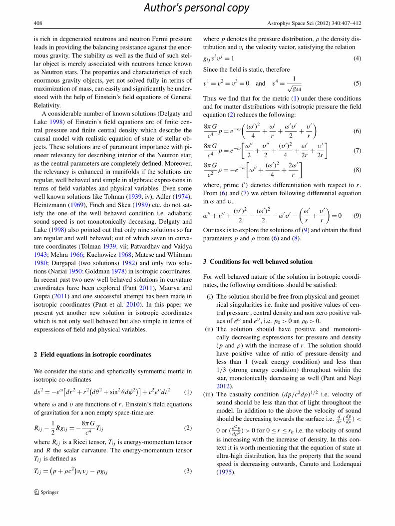
408 Astrophys Space Sci (2012) 340:407–412
is rich in degenerated neutrons and neutron Fermi pressureleads in providing the balancing resistance against the enor-mous gravity. The stability as well as the fluid of such stel-lar object is merely associated with neutrons hence knownas Neutron stars. The properties and characteristics of suchenormous gravity objects, yet not solved fully in terms ofmaximization of mass, can easily and significantly be under-stood with the help of Einstein’s field equations of GeneralRelativity.
A considerable number of known solutions (Delgaty andLake 1998) of Einstein’s field equations are of finite cen-tral pressure and finite central density which describe thecausal model with realistic equation of state of stellar ob-jects. These solutions are of paramount importance with pi-oneer relevancy for describing interior of the Neutron star,as the central parameters are completely defined. Moreover,the relevancy is enhanced in manifolds if the solutions areregular, well behaved and simple in algebraic expressions interms of field variables and physical variables. Even somewell known solutions like Tolman (1939, iv), Adler (1974),Heintzmann (1969), Finch and Skea (1989) etc. do not sat-isfy the one of the well behaved condition i.e. adiabaticsound speed is not monotonically deceasing. Delgaty andLake (1998) also pointed out that only nine solutions so farare regular and well behaved; out of which seven in curva-ture coordinates (Tolman 1939, vii; Patvardhav and Vaidya1943; Mehra 1966; Kuchowicz 1968; Matese and Whitman1980; Durgapal (two solutions) 1982) and only two solu-tions (Nariai 1950; Goldman 1978) in isotropic coordinates.In recent past two new well behaved solutions in curvaturecoordinates have been explored (Pant 2011), Maurya andGupta (2011) and one successful attempt has been made inisotropic coordinates (Pant et al. 2010). In this paper wepresent yet another new solution in isotropic coordinateswhich is not only well behaved but also simple in terms ofexpressions of field and physical variables.
2 Field equations in isotropic coordinates
We consider the static and spherically symmetric metric inisotropic co-ordinates
ds2 = −eω[dr2 + r2(dθ2 + sin2 θdφ2)] + c2eυdt2 (1)
where ω and υ are functions of r . Einstein’s field equationsof gravitation for a non empty space-time are
Rij − 1
2Rgij = −8πG
c4Tij (2)
where Rij is a Ricci tensor, Tij is energy-momentum tensorand R the scalar curvature. The energy-momentum tensorTij is defined as
Tij = (p + ρc2)vivj − pgij (3)
where p denotes the pressure distribution, ρ the density dis-tribution and vi the velocity vector, satisfying the relation
gij vivj = 1 (4)
Since the field is static, therefore
v1 = v2 = v3 = 0 and v4 = 1√g44
(5)
Thus we find that for the metric (1) under these conditionsand for matter distributions with isotropic pressure the fieldequation (2) reduces the following:
8πG
c4p = e−ω
((ω′)2
4+ ω′
r+ ω′υ ′
2+ υ ′
r
)(6)
8πG
c4p = e−ω
[ω′′
2+ υ ′′
2+ (υ ′)2
4+ ω′
2r+ υ ′
2r
](7)
8πG
c2ρ = −e−ω
[ω′′ + (ω′)2
4+ 2ω′
r
](8)
where, prime (′) denotes differentiation with respect to r .From (6) and (7) we obtain following differential equationin ω and υ .
ω′′ + ν′′ + (υ ′)2
2− (ω′)2
2− ω′υ ′ −
(ω′
r+ υ ′
r
)= 0 (9)
Our task is to explore the solutions of (9) and obtain the fluidparameters p and ρ from (6) and (8).
3 Conditions for well behaved solution
For well behaved nature of the solution in isotropic coordi-nates, the following conditions should be satisfied:
(i) The solution should be free from physical and geomet-rical singularities i.e. finite and positive values of cen-tral pressure , central density and non zero positive val-ues of eω and eυ , i.e. p0 > 0 an ρ0 > 0.
(ii) The solution should have positive and monotoni-cally decreasing expressions for pressure and density(p and ρ) with the increase of r . The solution shouldhave positive value of ratio of pressure-density andless than 1 (weak energy condition) and less than1/3 (strong energy condition) throughout within thestar, monotonically decreasing as well (Pant and Negi2012).
(iii) The casualty condition (dp/c2dρ)1/2 i.e. velocity ofsound should be less than that of light throughout themodel. In addition to the above the velocity of soundshould be decreasing towards the surface i.e. d
dr(dpdρ
) <
0 or (d2p
dρ2 ) > 0 for 0 ≤ r ≤ rb i.e. the velocity of soundis increasing with the increase of density. In this con-text it is worth mentioning that the equation of state atultra-high distribution, has the property that the soundspeed is decreasing outwards, Canuto and Lodenquai(1975).
Author's personal copy

Astrophys Space Sci (2012) 340:407–412 409
(iv) pρ
≤ dpdρ
, everywhere within the ball.
γ = d loge P
dogeρ= ρ
p
dp
dρ⇒ dp
dρ= γ
p
ρ,
for realistic matter γ ≥ 1 (Pant and Maurya 2012)(v) The red shift z should be positive, finite and monotoni-
cally decreasing in nature with the increase of r .
Under these conditions , we have to assume the one ofthe gravitational potential component in such a way that thefield equation (9) can be integrated and solution should bewell behaved. Further, the mass of the such modeled superdense object can be maximized by assuming surface density,ρb = 2 × 10¹⁴ g/cm3.
4 New class of solution
Equation (9) is solved by assuming
eω/2 = B(1 + Cr2)− 1
7 (10)
We get
eν2 = {1 + A(1 + Cr2)
17 }(1 + Cr2)
27
B2(11)
where A, B , and C are arbitrary constants.The expressions for pressure and density are given by
8πGρ
c2= 4
49B2(1 + Cr2)127
(21C + 6C2r2), (12)
8πGp
c4= 4
49B2(1 + Cr2)127
×[(7C + 4C2r2) + A(1 + Cr2)
17 (5C2r2 + 7C)
(1 + A(1 + Cr2)17 )
]
(13)
5 Properties of the new solution
The central values of pressure and density are given by(
8πGp
c4
)
0= 4
49B2
[7C + 7AC
(1 + A)
], (14)
(8πGρ
c2
)
0= 12C
7B2(15)
The central values of pressure and density will be nonzero positive definite, if the following conditions will be sat-isfied.
A > −1/2, C > 0 (16)
Subjecting the condition that positive value of ratio ofpressure-density and less than 1 at the centre i.e. p0
ρ0c2 ≤ 1
which leads to the following inequality,
1
3
[2A + 1
1 + A
]< 1 (17)
All the values of A which satisfy (16), will also lead tothe condition p0
ρ0c2 ≤ 1. Differentiating (13) with respect to r ,
dp
dr= 4
49B2{1 + A(1 + Cr2)17 }2(1 + Cr2)
197
⎡
⎢⎢⎣
A2(1 + Cr2) 27
(−30C2r − 90
7C3r3
)
+A(1 + Cr2) 1
7
(−44C2r − 120
7C3r3
)− 16C2r − 40
7C3r3
⎤
⎥⎥⎦ (18)
Thus extrema of p occur at the centre if
p′ = 0 ⇒ r = 0, (19)
8πG
c4
(p′′)
r=0 = 4
49B2
1
(1 + A)2
× [−30A2C2 − 44AC2 − 16C2] = −ve
(20)
Thus the expression of right hand side of (20) is nega-tive for all values of A satisfying (16), showing thereby thatthe pressure p is maximum at the centre and monotonicallydecreasing.
Now differentiating (12) with respect to r .
dρ
dr= 4C
49(1 + Cr2)197
[−60Cr − 60
7C2r3
](21)
Thus the extrema of ρ occur at the centre if
ρ′ = 0 ⇒ r = 0, (22)
8πG
c2
(ρ′′)
r=0 = −240C2
49B2(23)
Thus, the expressions of right hand side of (21) and (23)are negative showing thereby that the density ρ is maximumat the centre and monotonically decreasing.
The square of adiabatic sound speed at the centre,1c2 (
dpdρ
)r=0, is given by
Author's personal copy

410 Astrophys Space Sci (2012) 340:407–412
1
c2
(dp
dρ
)
r=0= 1
(1 + A)2
(15A2 + 22A + 8)
30
< 1 and positive (24)
The causality condition is obeyed at the centre for all val-ues of constant satisfying (16).
Further, it is mentioned here that the boundary of the su-per dense star is established only when −1/2 < A < 0.
6 Boundary conditions
The solutions so obtained are to be matched over the bound-ary with Schwarzschild exterior solution
ds2 =(
1 − 2GM
c2R
)c2dt2 −
(1 − 2GM
c2R
)−1
dR2
− R2dθ2 − R2 sin2 θdφ2 (25)
where M is the mass of the ball as determined by the ex-ternal observer and R is the radial coordinate of the exteriorregion. The usual boundary conditions are that the first andsecond fundamental forms are continuous over the boundaryr = rb or equivalently R = Rb . Thus we get,
eυb = 1 − 2GM
c2Rb
, (26)
Rb = rbeωb /2, (27)
1
2
(ω′ + 2
r
)
b
rb =(
1 − 2GM
c2Rb
)1/2
, (28)
1
2
(ν′)
brb = GM
c2Rb
(1 − 2
GM
c2Rb
)−1/2
(29)
Applying the boundary conditions we get the values ofthe arbitrary constants in terms of Schwarzschild parametersu = GM
c2Rband radius of the star Rb
A = 7u(1 + Cr2b ) − 4Cr2
b (1 − 2u)12
6Cr2b (1 + Cr2
b )17 (1 − 2u)
12 − 7u(1 + Cr2
b )87
, (30)
k =
√√√√√√{ 7u(1+Cr2
b )−4Cr2b (1−2u)
12
6Cr2b (1+Cr2
b )17 (1−2u)
12 −7u(1+Cr2
b )87}(1 + Cr2
b )17 + 1
√1 − 2u
(31)
where k = Rb
rb
B = k
[1 + 7{(1 − 2u)
12 − 1}
{5 − 7(1 − 2u)12 }
] 17
(32)
C = 7{(1 − 2u)12 − 1}
{5 − 7(1 − 2u)12 }r2
b
> 0 for u ≤ 0.244 (33)
Fig. 1 The variation of mass and radius of star with u
Fig. 2 The variation of p, ρ, p
ρc2 , 1c2 (
dpdρ
) from centre to surface foru = 0.186
Surface density is given by
8πG
c2ρb = 3
R2b
{8(1 − 2u)
12 − 8 + 10u
}> 0 (34)
Central red shift is given by
Z0 =[
B2
1 + A− 1
](35)
The surface red shift is given by
Zb = [(1 − 2u)−0.5 − 1
](36)
7 Application: slowly rotating structures and theirapplication to the Vela pulsars
For slowly rotating structure like the Vela pulsars (rotationvelocity about 70 rad/sec), one can calculate the momentof inertia in the first-order approximation which appears inthe Lense-Thrirring frame dragging effect. However, for thepresent case of an exact solution, it is very useful to applyan approximate, but very precise, empirical formula whichis based on the numerical results obtained for a large num-ber of theoretical equations of state (EOS) of dense nuclear
Author's personal copy

Astrophys Space Sci (2012) 340:407–412 411
Table 1 By assuming thesurface densityρb = 2 × 10¹⁴ g/cm3, thevariation of maximum Neutronstar mass, radius Rb , central redshift Z0 and surface red shiftZb = [(1 − 2u)−0.5 − 1] with u
u 8πGc2 ρbr
2b
MM�
Rb in km Z0 Zb I (g cm2)
.01 0.1161 0.026 3.973 0.0153 0.0102 0.003 × 1045
.02 0.2243 0.075 5.560 0.0315 0.0206 0.0187 × 1045
.04 0.4175 0.2072 7.686 0.0667 0.0426 0.1005 × 1045
.06 0.5793 0.3710 9.183 0.1063 0.066 0.2603 × 1045
.08 0.7100 0.5564 10.318 0.1513 0.0911 0.499 × 1045
.1 0.8094 0.7549 11.190 0.2033 0.1180 0.807 × 1045
.15 0.9229 1.262 12.479 0.3807 0.1953 1.73 × 1045
.175 0.9084 1.498 12.688 0.5150 0.2401 2.15 × 1045
.186 0.8874 1.591 12.685 0.5933 0.2618 2.30 × 1045
Table 2 The march of pressure,density, pressure-density ratio,red shift and square of adiabaticsound speed and adiabatic indexwithin the ball corresponding tou = 0.186
r/rb8πG
c4 pr2b
8πG
c2 ρr2b
p
ρc21c2 (
dpdρ
) γ = dpdρ
/pρ
Z
0 0.5745 4.654 0.1234 0.15394 1.247 0.5933
0.1 0.5482 4.483 0.1222 0.15393 1.258 0.5852
0.2 0.4790 4.033 0.1187 0.15388 1.295 0.5623
0.3 0.3882 3.443 0.1127 0.15377 1.363 0.5286
0.4 0.2962 2.84 0.1041 0.15353 1.474 0.4887
0.5 0.2147 2.313 0.0928 0.15307 1.649 0.4463
0.6 0.1479 1.876 0.0788 0.15228 1.930 0.4044
0.7 0.0954 1.530 0.0623 0.15107 2.421 0.3644
0.8 0.0549 1.260 0.0435 0.14935 3.428 0.3271
0.9 0.0238 1.050 0.0226 0.14706 6.486 0.2929
1.0 0.000 0.8874 0.0000 0.14419 ∞ 0.2618
matter. For the type of solution considered in the presentstudy, the formula yields in the following form (Bejger andHaensel 2002; Pant and Negi 2012).
I = (2/5)(1 + y)MR2; (37)
where y is the dimensionless compactness parameter mea-sured in units of M� (in km)/km, i.e.
y = (M/R)/M� (in km) km−1 (38)
With the help of (37), we can calculate the moment of in-ertia, for various super dense objects as shown in Tables 1and 2. These values of masses and moment of inertia agreequite well with those of the masses and the moment of iner-tia calculated for the Vela pulsars.
8 Discussions and conclusions
It has been observed that the physical parameters(p,ρ,
p
ρc2 , z) are positive at the centre and within the limitof realistic state equation and monotonically decreasingfor 0.244 > u > 0. However, corresponding to any valueof 0.244 > u > 0.186, though the causality condition isobeyed throughout within the ball but the trend of adiabatic
sound speed is erratic. Thus, the solution is well behavedfor all values of u satisfying the inequality 0. < u ≤ 0.186.We now here present a model of super dense star basedon the particular solution discussed above by assumingsurface density; ρb = 2 × 10¹⁴ g/cm3. Corresponding tou = 0.186, the resulting well behaved model has maximummass M = 1.591 M� with radius Rb ≈ 12.685 km (seeFig. 1 and Fig. 2). The model has mass within the rangeof neutron star. The good matching of our results for Velapulsars show the robustness of our model.
Acknowledgements One of us (Neeraj Pant) acknowledges his grat-itude to Lt. Gen. Jatinder Singh AVSM**, SM, Comdt, NDA for hismotivation and encouragement. Neeraj Pant also extends his gratitudeto Prof. O.P. Shukla, Principal NDA, for his encouragement.
Authors are grateful to the anonymous referee for his relevant sug-gestions.
References
Adler, R.J.: J. Math. Phys. 15, 727 (1974)Bejger, M., Haensel, P.: Astron. Astrophys. 396, 917 (2002)Canuto, V., Lodenquai, J.: Phys. Rev. C 12, 2033 (1975)Delgaty, M.S.R., Lake, K.: Comput. Phys. Commun. 115, 395 (1998)Durgapal, M.C.: J. Phys. A, Math. Gen. 15, 2637 (1982)Finch, M., Skea, J.E.F.: Class. Quantum Gravity 4, 467 (1989)
Author's personal copy

412 Astrophys Space Sci (2012) 340:407–412
Goldman, S.P.: Astrophys. J. 226, 1079 (1978)Heintzmann, H.: Z. Phys. 228, 489 (1969)Kuchowicz, B.: Acta Phys. Pol. 34, 131 (1968)Matese, J.J., Whitman, P.G.: Phys. Rev. D, Part. Fields 22, 1270 (1980)Maurya, S.K., Gupta, Y.K.: Astrophys. Space Sci. 334, 145 (2011).
doi:10.1007s10509-011-0705-yMehra, A.L.: J. Aust. Math. Soc. 6, 153 (1966)Nariai: Sci. Rep. Tohoku Univ., Ser. 1 34, 160 (1950)
Pant, N.: Astrophys. Space Sci. 331, 633 (2011)Pant, N., Negi, P.S.: Astrophys. Space Sci. 338, 163 (2012)Pant, N., et al.: Astrophys. Space Sci. 330, 353 (2010)Pant, N., Maurya, S.K.: Appl. Math. Comput. 218, 8260 (2012).
doi:10.1016/j.amc.2012.01.044Patvardhav, Vaidya: J. Univ. Bombay 12(Part III), 23 (1943)Tolman, R.C.: Phys. Rev. 55, 364 (1939)
Author's personal copy

1 23
Astrophysics and Space ScienceAn International Journal of Astronomy,Astrophysics and Space Science ISSN 0004-640XVolume 341Number 2 Astrophys Space Sci (2012) 341:469-475DOI 10.1007/s10509-012-1105-7
A family of charge analogue of Durgapalsolution
Pratibha Fuloria & B. C. Tewari

1 23
Your article is protected by copyright and
all rights are held exclusively by Springer
Science+Business Media B.V.. This e-offprint
is for personal use only and shall not be self-
archived in electronic repositories. If you
wish to self-archive your work, please use the
accepted author’s version for posting to your
own website or your institution’s repository.
You may further deposit the accepted author’s
version on a funder’s repository at a funder’s
request, provided it is not made publicly
available until 12 months after publication.

Astrophys Space Sci (2012) 341:469–475DOI 10.1007/s10509-012-1105-7
O R I G I NA L A RT I C L E
A family of charge analogue of Durgapal solution
Pratibha Fuloria · B.C. Tewari
Received: 26 March 2012 / Accepted: 1 May 2012 / Published online: 16 May 2012© Springer Science+Business Media B.V. 2012
Abstract We obtain a new parametric class of exact solu-tions of Einstein–Maxwell field equations which are wellbehaved. We present a charged super-dense star model af-ter prescribing particular forms of the metric potential andelectric intensity. The metric describing the super densestars joins smoothly with the Reissner–Nordstrom metricat the pressure free boundary. The electric density assumed
is E2
c1= Kx
2 (1 + x)n(1 + 6x)23 where n may take the val-
ues 0,1,2,3,4 and so on and K is a positive constant. Forn = 0,1 we rediscover the solutions by Gupta and Maurya(Astrophys. Space Sci. 334(1):155, 2011) and Fuloria et al.(J. Math. 2:1156, 2011) respectively. The solution for n = 2have been discussed extensively keeping in view of well be-haved nature of the charged solution of Einstein–Maxwellfield equations. The solution for n = 3 and n = 4 can be alsostudied likewise. In absence of the charge we are left behindwith the regular and well behaved fifth model of Durgapal (J.Phys. A 15:2637, 1982). The outmarch of pressure, density,pressure-density ratio and the velocity of sound is monoton-ically decreasing, however, the electric intensity is mono-tonically increasing in nature. For this class of solutions themass of a star is maximized with all degree of suitability,compatible with Neutron stars and Pulsars.
By assuming the surface density ρb = 2 × 10¹⁴ g/cm3
(Brecher and Caporaso in Nature 259:377, 1976), corre-sponding to K = 12 with X = 0.1, the resulting well be-haved model has the mass M = 2.12M�, radius Rb ≈
P. Fuloria (�)Physics Deptt., S.S.J. Campus, Almora, Indiae-mail: [email protected]
B.C. TewariMath Deptt., S.S.J. Campus, Almora, Indiae-mail: [email protected]
16.07 km and moment of inertia I = 4.95 × 1045 g cm2; forK = 8 with X = 0.1, the resulting well behaved model hasthe mass M = 1.50M�, radius Rb ≈ 16.78 km and momentof inertia I = 3.68 × 1045 g cm2. These values of massesand moment of inertia are found to be consistent with othermodels of Neutron stars and Pulsars available in the litera-ture and are applicable for the Crab Pulsars.
Keywords General relativity · Reissner–Nordstrom ·Einstein–Maxwell · Charged fluid spheres
1 Introduction
Exact solutions with well-behaved nature of Einstein–Maxwell field equations are of vital importance in rela-tivistic astrophysics. Such solutions may be used to makea suitable model of super dense object with charge mat-ter like Neutron star, quark star, pulsar and analogous stars.It is interesting to observe that, in the presence of charge,the gravitational collapse of a spherical symmetric distri-bution of the matter to a point singularity may be avoidedbecause the presence of some charge in a spherical ma-terial distribution provides an additional resistance againstthe gravitational contraction by means of electric repulsion.The inclusion of charge plays very important role in thestability of massive fluid spheres. A spherical fluid distri-bution of uniform density with a net charge on the sur-face is more stable than a surface without charge (de Fe-lice et al. 1995). Thus a stable massive charged configu-ration can be produced in which repulsive force from thecharge counter balances the gravitational attraction. Thesingularities which appear in the Schwarzschild solutioncorresponding to spherically symmetric static perfect fluiddistribution can be avoided to a great extent by including
Author's personal copy

470 Astrophys Space Sci (2012) 341:469–475
charge in them. The negative pressure of Bayin’s solution(1978) makes it physically unreasonable, however the in-clusion of charge in Bayin’s solution makes it physicallyreasonable i.e. the pressure is a decreasing function of ra-dius from centre to surface (Ray et al. 2007). Bonnor (1965)has shown that dust cloud of arbitrarily Large mass andsmall radius can remain in equilibrium if it has an elec-tric charge density related to the mass density by σ = ±ρ.Usmani et al. (2011) have shown that the de Sitter void ofa charged gravastar, represents the same thing as electro-magnetic mass model which is generating the gravitationalmass and provides stability to the astrophysical configura-tion. All these advantages of charged spherical models mo-tivated us to consider the charge analogue of Durgapal’ so-lution (1982). We have found out a new parametric classof exact solutions of Einstein–Maxwell field equations fora static, spherically symmetric distribution of the chargedand perfect fluid with well behaved nature and to constructa suitable model of super dense object with charge matter.Many of the authors electrified the well known unchargedfluid spheres e.g. Durgapal and Fuloria (1985) solution byGupta and Maurya (2010), Schwarzschild solution by Guptaand Gupta (1986) and by Gupta and Kumar (2005), Ku-chowich (1968) solution by Nduka (1977), Tolman (1939)solution by Cataldo and Mitskievic (1992) and Pant andNegi (2012), Heintzmann’s solution (1969) by Pant et al.(2011), Pant and Maurya (2012), Adler’s (1974) solutionby Pant and Tewari (2011), Pant et al. (2011) and so on.We have tried to charge the Durgapal (1982) solution byassuming a parametric expression for electric density. Forthe values of n = 0,1,2 the solutions are well behaved. Thesolutions for the n = 3, n = 4 may be obtained and theirwell behaved nature may be verified by applying the variousconditions.
For well behaved nature of the solution the followingconditions should be satisfied: Delgaty and Lake (1998) andPant et al. (2010).
(i) The solution should be free from physical and geo-metrical singularities i.e. finite and positive values of centralpressure, central density and non zero positive values of eλ
and eυ .(ii) The solution should have positive and monotonically
decreasing expressions for pressure and density (p and ρ)with the increase of r . The solution should have positivevalue of ratio of pressure-density and less than 1 (weak en-ergy condition) and less than 1/3 (strong energy condition)throughout within the star, monotonically decreasing as well(Pant and Negi 2012).
(iii) The casualty condition (dp/c2dρ)1/2 i.e. velocity ofsound should be less than that of light throughout the model.In addition to the above the velocity of sound should be.
Decreasing towards the surface i.e. ddr
(dpdρ
) < 0 or
(d2p
dρ2 ) > 0 for 0 ≤ r ≤ rb i.e. the velocity of sound is in-
creasing with the increase of density. In this context it isworth mentioning that the equation of state at ultra-high dis-tribution, has the property that the sound speed is decreasingoutwards.
(iv) pρ
≤ dpdρ
, everywhere within the ball. γ = d loge P
loge ρ=
ρp
dpdρ
⇒ dpdρ
= γpρ
, for realistic matter γ ≥ 1 (Pant and Mau-rya 2012).
(v) The red shift z should be positive, finite and mono-tonically decreasing in nature with the increase of r .
(vi) Electric intensity E is positive and monotonically in-creasing from centre to boundary and at the centre the Elec-tric intensity is zero.
2 Einstein–Maxwell equation for charged fluiddistribution
Let us consider a spherical symmetric metric in curvaturecoordinates
ds2 = −eλdr2 − r2(dθ2 + r2 sin2 θdφ2) + eνdt2 (1)
where the functions λ(r) and ν(r) satisfy the Einstein–Maxwell equations
−8πG
c4T i
j = Rij − 1
2Rδi
j
= −8πG
c4
[(c2ρ + p
)vivj − pδi
j
+ 1
4π
(−F imFjm + 1
4δijFmnF
mn
)](2)
where ρ, p, vi , Fij denote energy density, fluid pressure, ve-locity vector and skew-symmetric electromagnetic field ten-sor respectively.
In view of the metric (1), the field equation (2) givesDionysiou (1982)
ν′
re−λ − (1 − e−λ)
r2= 8πG
c4p − q2
r4(3)
(ν′′
2− λ′ν′
4+ ν′2
4+ ν′ − λ′
2r
)e−λ = 8πG
c4p + q2
r4(4)
λ′
re−λ + (1 − e−λ)
r2= 8πG
c2ρ + q2
r4(5)
where prime (′) denotes the differentiation with respect to r
and q(r) represents the total charge contained with in thesphere of radius r .
By using the transformation
eν = B(1 + x)5, x = c1r2 and e−λ = Z. (6)
where B being the positive constant. Now putting (6) into(3)–(5), we have
Author's personal copy

Astrophys Space Sci (2012) 341:469–475 471
10Z
(1 + x)− (1 − Z)
x+ c1q
2
x2= 1
c1
8πGP
c4(7)
(1 − Z)
x− 2
dZ
dX+ c1q
2
x2= 1
c1
8πGρ
c4(8)
and Z satisfying the equation
dZ
dx+ 14x2 − 2x − 1
x(1 + x)(1 + 6x)xZ = {(2q2c1/x) − 1}(1 + x)
x(1 + 6x)
(9)
where x = c1r2, e−λ = Z.
3 New class of solutions
In order to solve the differential equation (9) let us considerthe electric intensity E of the following form
E2
c1= c1q
2
x2= Kx
2(1 + x)n(1 + 6x)
23 (10)
where K is a positive constant. The electric density is soassumed that the model is physically significant and well
behaved i.e. E remains regular and positive throughout thesphere.
In view of (10) differential equation (9) yields the follow-ing solution
e−λ = K
(5 + n)
x(1 + x)2+n
(1 + 6x)1/3
+ 1
(1 + x)3
[1 − x(309 + 54x + 8x2)
112
]
+ Ax
(1 + 6x)13
(1 + x)3 (11)
where A is an arbitrary constant of integration.
4 Properties of the new class of solutions
Using (11), into (7) and (8), we get the following expres-sions for pressure and energy density
1
c1
8πG
c4p = 1
(1 + x)4
[(475 − 4125x − 1050x2 − 200x3)
112+ A(1 + 11x)
(1 + 6x)13
]+ K (1 + x)n(2 + (n + 29)x + (52 + 6n)x2)
2(5 + n)(1 + 6x) 13
(12)1
c1
8πG
c4p0 =
(475
112+ A + K
(5 + n)
)(13)
1
c1
8πG
c2ρ = 1
(1 + x)4
[(1935 + 15x + 450x2 + 120x3)
112− A
(3 + 11x − 22x2)
(1 + 6x)43
]
− K(1 + x)n{6 + (53 + 5n)x + (178 + 40n)x2 + (256 + 60n)x3}2(5 + n)(1 + 6x)
43
(14)
1
c1
8πG
c2ρ0 =
(1935
112− 3A − 6K
2(5 + n)
)(15)
Differentiating (12) and (14) w.r.t. x, we get:
1
c1
8πG
c4
dp
dx= − 25(241 − 411x − 60x2 − 8x3)
112(1 + x)5+ 5A(1 − 3x − 44x2)
(1 + x)5(1 + 6x)43
+
(K(1 + x)n−1[(25 + 3n) + (245 + 58n + n2)x+(740 + 302n + 12n2)x2 + (520 + 372n + 36n2)x3]
)
2(5 + n)(1 + 6x) 43
(16)
1
c1
8πG
c2
dρ
dx= −15
112(1 + x)5(515 − 57x + 36x2 + 8x3) + 5A
(1 + x)5(1 + 6x)73
(5 + 39x + 66x2 − 88x3)
− K(1 + x)n−1
2(5 + n)(1 + 6x)73
((5 + 11n) + (255 + 164n + 5n2)x + (1730 + 906n + 70n2)x2
+(4040 + 2264n + 300n2)x3 + (2560 + 2136n + 360n2)x4
)(17)
1
c2
dp
dρ= − (1 + 6x) [K(1 + x)n+4N(x) − 50/112P(x)(1 + 6x)4/3(5 + n) + 10AQ(x)(5 + n)]
[K(1 + x)n+4M(x) − 30/112H(x)(1 + 6x)7/3(5 + n) + 10AT (x)(5 + n)] (18)
Author's personal copy

472 Astrophys Space Sci (2012) 341:469–475
where
H(x) = 515 − 57x + 36x2 + 8x3 T (x) = 5 + 39x + 66x2 − 88x3
M(x) = (5 + 11n) + (255 + 164n + 5n2)x + (1730 + 906n + 70n2)x2 + (4040 + 2264n + 300n2)x3
+ (2560 + 2136n + 360n2)x4
N(x) = (25 + 3n) + (245 + 58n + n2)x + (
740 + 320n + 12n2)x2 + (520 + 372n + 36n2)x3
P(x) = 241 − 411x − 60x2 − 8x3 Q(x) = 1 − 3x − 44x2
(1
c2
dp
dρ
)
0= −
[31K − 6025
56 (5 + n) + 10A(5 + n)]
[27K − 7725
56 (5 + n) + 50A(5 + n)] (19)
5 Variety of classes of solutions
Case 1 When n = 0, Gupta and Maurya Solution (2011)The resulting Solution is
e−λ = K
5
x(1 + x)2
(1 + 6x)1/3
+ 1
(1 + x)3
[1 − x(309 + 54x + 8x2)
112
]
+ Ax
(1 + 6x)13
(1 + x)−3 (20)
where A is an arbitrary constant of integrationThe expressions for pressure and energy density are given
by
1
c1
8πG
c4p = 1
(1 + x)4
[(475 − 4125x − 1050x2 − 200x3)
112
+ A(1 + 11x)
(1 + 6x)13
]+ K
10
(2 + 29x + 52x2)
(1 + 6x) 13
(21)
1
c1
8πG
c2ρ = 1
(1 + x)4
[(1935 + 15x + 450x2 + 120x3)
112
− A(3 + 11x − 22x2)
(1 + 6x)43
]− K
10
× (6 + 53x + 178x2 + 256x3)
(1 + 6x)43
(22)
The solution gives wide range of constant K (0 < K ≤ 50)for which the solution is well behaved and therefore suitablefor modelling of superdense star.Case 2 When n = 1 Fuloria et al. (2011) solution
The resulting Solution is
e−λ = K
6
x(1 + x)3
(1 + 6x)1/3
+ 1
(1 + x)3
[1 − x(309 + 54x + 8x2)
112
]
+ Ax
(1 + 6x)13
(1 + x)3 (23)
where A is an arbitrary constant of integration.
The expression for pressure and density are expressed as,
1
c1
8πG
c4p = 1
(1 + x)4
[(475 − 4125x − 1050x2 − 200x3)
112
+ A(1 + 11x)
(1 + 6x)13
]
+ K
6
(1 + x)(1 + 15x + 29x2)
(1 + 6x) 13
(24)
1
c1
8πG
c2ρ = 1
(1 + x)4
[(1935 + 15x + 450x2 + 120x3)
112
− A(3 + 11x − 22x2)
(1 + 6x)43
]
− K
6
(1 + x)(3 + 29x + 109x2 + 158x3)
(1 + 6x)43
(25)
The solution is well behaved for all the values of K satisfy-ing the inequality 0 < K < 10 and X = 0.2.
6 New well behaved solution
Case 3 When n = 2We have the expression for electric density as
E2
c1= 1
2Kx(1 + x)2(1 + 6x)
23 (26)
(d
dx
E2
c1
)
x=0= K
2(27)
The electric intensity is minimum at the centre and mono-tonically increasing for all values K > 0. Also at the centreit is zero. Thus we have, K ≥ 0, c1 > 0.
In view of (26) differential equation (9) yields the follow-ing solution
e−λ = K
7
x(1 + x)4
(1 + 6x)1/3
+ 1
(1 + x)3
[1 − x(309 + 54x + 8x2)
112
]
+ Ax
(1 + 6x)13
(1 + x)−3 (28)
Author's personal copy
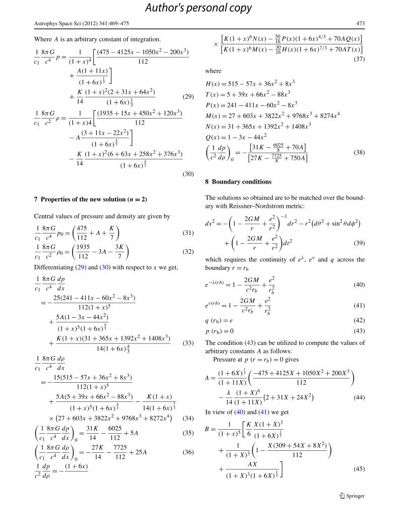
Astrophys Space Sci (2012) 341:469–475 473
Where A is an arbitrary constant of integration.
1
c1
8πG
c4p = 1
(1 + x)4
[(475 − 4125x − 1050x2 − 200x3)
112
+ A(1 + 11x)
(1 + 6x)13
]
+ K
14
(1 + x)2(2 + 31x + 64x2)
(1 + 6x) 13
(29)
1
c1
8πG
c2ρ = 1
(1 + x)4
[(1935 + 15x + 450x2 + 120x3)
112
− A(3 + 11x − 22x2)
(1 + 6x)43
]
− K
14
(1 + x)2(6 + 63x + 258x2 + 376x3)
(1 + 6x)43
(30)
7 Properties of the new solution (n = 2)
Central values of pressure and density are given by
1
c1
8πG
c4p0 =
(475
112+ A + K
7
)(31)
1
c1
8πG
c2ρ0 =
(1935
112− 3A − 3K
7
)(32)
Differentiating (29) and (30) with respect to x we get,
1
c1
8πG
c4
dp
dx
= −25(241 − 411x − 60x2 − 8x3)
112(1 + x)5
+ 5A(1 − 3x − 44x2)
(1 + x)5(1 + 6x)43
+ K(1 + x)(31 + 365x + 1392x2 + 1408x3)
14(1 + 6x) 43
(33)
1
c1
8πG
c4
dρ
dx
= −15(515 − 57x + 36x2 + 8x3)
112(1 + x)5
+ 5A(5 + 39x + 66x2 − 88x3)
(1 + x)5(1 + 6x)43
− K(1 + x)
14(1 + 6x)73
× (27 + 603x + 3822x2 + 9768x3 + 8272x4) (34)
(1
c1
8πG
c4
dp
dx
)
0= 31K
14− 6025
112+ 5A (35)
(1
c1
8πG
c4
dρ
dx
)
0= −27K
14− 7725
112+ 25A (36)
1
c2
dp
dρ= − (1 + 6x)
×[K(1 + x)6N(x) − 50
16P(x)(1 + 6x)4/3 + 70AQ(x)]
[K(1 + x)6M(x) − 30
16H(x)(1 + 6x)7/3 + 70AT (x)]
(37)
where
H(x) = 515 − 57x + 36x2 + 8x3
T (x) = 5 + 39x + 66x2 − 88x3
P(x) = 241 − 411x − 60x2 − 8x3
M(x) = 27 + 603x + 3822x2 + 9768x3 + 8274x4
N(x) = 31 + 365x + 1392x2 + 1408x3
Q(x) = 1 − 3x − 44x2
(1
c2
dp
dρ
)
0= −
[31K − 6025
8 + 70A]
[27K − 7725
8 + 750A] (38)
8 Boundary conditions
The solutions so obtained are to be matched over the bound-ary with Reissner–Nordstrom metric:
ds2 = −(
1 − 2GM
r+ e2
r2
)−1
dr2 − r2(dθ2 + sin2 θdφ2)
+(
1 − 2GM
r+ e2
r2
)dt2 (39)
which requires the continuity of eλ, eν and q across theboundary r = rb
e−λ(rb) = 1 − 2GM
c2rb+ e2
r2b
(40)
eν(rb) = 1 − 2GM
c2rb+ e2
r2b
(41)
q (rb) = e (42)
p (rb) = 0 (43)
The condition (43) can be utilized to compute the values ofarbitrary constants A as follows:
Pressure at p (r = rb) = 0 gives
A = (1 + 6X)13
(1 + 11X)
(−475 + 4125X + 1050X2 + 200X3
112
)
− k
14
(1 + X)6
(1 + 11X)
(2 + 31X + 24X2) (44)
In view of (40) and (41) we get
B = 1
(1 + x)5
[K
6
X(1 + X)3
(1 + 6X)13
+ 1
(1 + X)3
(1 − X(309 + 54X + 8X2)
112
)
+ AX
(1 + X)3(1 + 6X)13
](45)
Author's personal copy

474 Astrophys Space Sci (2012) 341:469–475
Table 1 The variation of various physical parameters at the centre, surface density, electric field intensity on the boundary, mass and radius ofstars with different values of K and X = 0.1
K 1c1
8πG
c4 p01c1
8πG
c2 ρ01c2
p0ρ0
1c2 (
dpdρ
)x=0 z0 ( E2
c1)rb
8πG
c2 ρbr2b
MM� ≈ rb in km
2 3.5774 19.2676 0.1856 0.5603 0.31 0.150 1.177 0.49 17.78
4 3.17103 20.4857 0.1548 0.4514 0.34 0.300 1.343 0.84 17.45
6 2.7653 21.7039 0.12741 0.3757 0.38 0.451 1.091 1.17 17.12
8 2.3593 22.922 0.1029 0.3199 0.42 0.601 1.048 1.50 16.78
10 1.9538 24.1401 0.08091 0.2772 0.45 0.752 1.005 1.80 16.43
12 1.5472 25.3582 0.0610 0.2434 0.50 0.902 0.9624 2.12 16.07
14 1.1412 26.5763 0.04294 0.2161 0.55 1.053 0.919 2.37 15.71
16 0.7332 27.7944 0.02645 0.1934 0.60 1.203 0.876 2.63 15.34
Table 2 The march of pressure, density, pressure-density ratio, square of adiabatic sound speed, red shift, electric intensity within the perfect fluidsphere corresponding to K = 1 and X = 0.2
r/rb8πG
c4 pr2b
8πG
c2 ρr2b
p
ρc21c2 (
dpdρ
) z (E2
c1)
0.0 1.019 2.9429 0.3462 0.9748 1.6410 0.0000
0.1 0.999 2.9217 0.3422 0.9688 1.6279 0.0010
0.3 0.855 2.7562 0.3105 0.9245 1.5258 0.0099
0.4 0.7420 2.6176 0.2834 0.8890 1.4410 0.01915
0.5 0.6106 2.4480 0.2494 0.8462 1.3378 0.03283
0.6 0.4709 2.2535 0.2089 0.7960 1.2197 0.05256
0.7 0.3320 2.0408 0.1627 0.7375 1.0906 0.08040
0.8 0.2025 1.8162 0.1115 0.6680 0.9543 0.11906
0.9 0.0898 1.5853 0.0566 0.5829 0.8145 0.17198
1.0 0.0000 1.3521 0.0000 0.4712 0.6742 0.24358
The expression for mass can be written as
GM
c2= rb
2
[1 + K
2X2(1 + X)2(1 + 6X)
23 − B(1 + X)5
]
(46)
The expression for surface density is given by
8πG
c2ρbr
2b = 1
(1 + X)4
[(1935 + 15X + 450X2 − 120X3)
112
− A(3 + 11X − 22X2)
(1 + 6X)43
]
− K
6
(1 + X)(3 + 29X + 109X2 + 158X3)
(1 + 6X)43
(47)
In view of Table 1 we observe that pressure, density,pressure density ratio, red shift, electric density all is pos-itive at the centre. Assuming the surface density ρb = 2 ×10¹⁴ g/cm3 the mass and radius has been calculated for dif-ferent values of K and X = 0.1.
In view of the Table 2 we observe that pressure, density,pressure-density ratio and square of adiabatic sound speed
and red-shift decrease monotonically with the increase ofradial coordinate and electric intensity increases monotoni-cally with the increase of radial coordinate within the per-fect fluid sphere. At the centre of the star the matter is sodense that electrons are forced to combine with protons re-sulting into neutrons and neutrinos. This process favours themaximum matter at the centre to be neutral i.e. the electricintensity will be zero at the centre. As we move towardssurface the density goes on decreasing approaching zero atthe surface. The possibility of combination of electrons andprotons becomes less and less as we move towards surface,hence the electric intensity will be maximum towards thesurface.
9 Slowly rotating structures and their application toCrab Pulsars
For slowly rotating structures like the Crab pulsars (rotationvelocity about 188 rad/sec) we can calculate the momentof inertia in the first-order approximation which appears inthe Lense–Thrirring frame dragging effect. However, for the
Author's personal copy
Astrophys Space Sci (2012) 341:469–475 475
exact solution that we have considered here, it is very use-ful to apply an approximate, but very precise, empirical for-mula which is based on the numerical results obtained for alarge number of theoretical equations of state of dense nu-clear matter.
For the type of solution considered in the present study,the formula yields in the following form (Bejger andHaensel 2002):
I = (2.5)(1 + u)MR2; (48)
where u is the dimensionless compactness parameter mea-sured in units of MΘ (in km)/km, i.e.
u = (M/R)/M� (in km) km−1 (49)
Equation (48) is used to calculate the moment of iner-tia for the models presented in Table 1. Corresponding toM = 2.12 M� and R = 16.07 km we obtain the moment ofinertia for the configuration as 4.95 × 1045 gm cm2. For themass 1.50 M� and R = 16.78 km equation (48) yields themoment of inertia as 3.68 × 1045 gm cm2.
These values of masses and moment of inertia agree quitewell with those of the masses and the moment of inertia cal-culated for the Crab pulsars on the basis of newly estimatedvalue of Crab nebula mass M = 4.6M� (Bejger and Haensel2002; and Pant and Negi 2012).
10 Results and discussions
We have electrified the uncharged fluid sphere e.g. Durga-pal (1982) Vth solution. The charged solution is well be-haved with positive values of charge parameter K and com-pletely describes interior of the super-dense astrophysicalobjects with charge matter. The electric density assumed isE2
c1= c1q
2
x2 = Kx2 (1 + x)n(1 + 6x)
23 . The electric density is
so assumed that the model is physically significant and wellbehaved. E vanishes at the centre of the star and increasesas we move towards the surface and is positive throughoutthe star. In view of Table 1 it has been observed that all thephysical parameters (p,ρ,
p
ρc2 , Z and E2
c1) are positive at the
centre and within the limit of realistic equation of state.We observe that with the increase of the value of n, al-
though the solutions become more complicated in terms ofexpressions, but they show the well behaved nature and sat-isfy all the necessary conditions to be physically realizable.Thus by assigning different positive integral value to param-eter n we get a variety of classes of exact solutions. We haveobtained a generalized solution of Einstein–Maxwell fieldequations of general relativity for a static, spherically sym-metric distribution of the charged fluid with well behavednature.
For n = 0 we get the Gupta and Maurya (2011) solution,which is well behaved for a wide range of constant K .
For n = 1, we get the Fuloria et al. (2011) solution whichis also well behaved for K < 10 hence, suitable for modelingof super dense star.
For n = 2, we have obtained a new solution which hasbeen studied in detail exposing its well behaved nature. Thesolution is well behaved for a wide range of constant K .
For this class of solution (n = 2) the mass of a star ismaximized with all degree of suitability compatible withquark stars, neutron stars and pulsars. By assuming the sur-face density ρb = 2 × 10¹⁴ g/cm3 corresponding to K = 12and X = 0.1 the maximum mass of the star comes outto be 2.12M� with its radius 16.07 km. Correspondingto this model we obtain the moment of inertia as 4.95 ×1045 gm cm2. The values of mass, radius and moment of in-ertia obtained in the present study strongly favour our modelto represent the crab pulsar. In absence of the charge we areleft behind with the regular and well behaved fifth model ofDurgapal (1982).
Acknowledgements Authors acknowledge their gratitude to Dr.Neeraj Pant (Associate Professor) Maths Deptt., National DefenseAcademy Khadakwasla, Pune for his stimulating discussions and mo-tivation. Authors are also grateful to the referee for pointing out theerrors in original manuscript and making constructive suggestions.
References
Adler, R.J.: J. Math. Phys. 15(6), 727 (1974)Bayin, S.S.: Phys. Rev. D 18, 2745 (1978)Bejger, M., Haensel, P.: Astron. Astrophys. 396, 917 (2002)Bonnor, W.B.: Mon. Not. R. Astron. Soc. 129, 443 (1965)Brecher, K., Caporaso, G.: Nature 259, 377 (1976)Cataldo, M., Mitskievic, N.V.: Class. Quantum Gravity 9, 545 (1992)de Felice, F., Yu, Y., Fang, J.: Mon. Not. R. Astron. Soc. 277, L17
(1995)Delgaty, M.S.R., Lake, K.: Comput. Phys. Commun. 115, 395 (1998)Dionysiou, D.D.: Astrophys. Space Sci. 85, 331 (1982)Durgapal, M.C.: J. Phys. A, Math. Gen. 15, 2637 (1982)Durgapal, M.C., Fuloria, R.S.: Gen. Relativ. Gravit. 17, 671 (1985)Fuloria, P., Tiwari, B.C., Joshi, B.C.: J. Mod. Phys. 2, 1156 (2011)Gupta, Y.K., Gupta, R.S.: Acta Phys. Pol. B 17, 855 (1986)Gupta, Y.K., Kumar, M.: Astrophys. Space Sci. 299(1), 43 (2005)Gupta, Y.K., Maurya, S.K.: Astrophys. Space Sci. (2010). doi:10.1007/
s10509-010-0445-4Gupta, Y.K., Maurya, S.K.: Astrophys. Space Sci. 334(1), 155 (2011)Heintzmann, H.: Z. Phys. 228, 489 (1969)Kuchowich, B.: Acta Phys. Pol. 33, 541 (1968)Nduka, A.: Acta Phys. Pol. B 8, 75 (1977)Pant, N., Maurya, S.K.: Appl. Math. Comput. 218, 8260 (2012)Pant, N., Negi, P.S.: Astrophys. Space Sci. 338(2), 163 (2012)Pant, M.J., Tewari, B.C.: J. Mod. Phys. 2(5), 481 (2011)Pant, N., et al.: Astrophys. Space Sci. 330(2), 353 (2010)Pant, N., Tewari, B.C., Fuloria, P.: J. Mod. Phys. 2(12), 1538 (2011)Ray, S., et al.: Int. J. Mod. Phys. D 16, 1745 (2007)Tolman, R.C.: Phys. Rev. 55, 367 (1939)Usmani, A.A., et al.: Phys. Lett. B 701, 388 (2011)
Author's personal copy