DOCUMENT RESUME

ED 142 355 RC 010 032

AUTHOR Hartman, John J.TITLE Rural-Urban Differences in Drinking Driving Behavior;

Attitudes and Perceptions of Kansas Youth.INSTITUTION Wichita Dept. of Community Health, Kan.SPONS AGENCY National Highway Traffic Safety Administration (DOT),

Washington, D. C.

PUB DATE Sep 77CONTRACT DOT-NS-054-1-070NOTE 29p.; Paper presented at the Annual Meeting of the

Rural Sociological Society (Madison, Wisconsin,September 1977)

EDRS PRICE MF-$0.83 HC-$2.06 Plus Postage.DESCRIPTORS Age; Alcoholism; American Indians; Behavior; Black

Youth; Caucasians; Comparative Analysis; *Drinking;Family Income; *High School Students; InstructionalProgram Divisions; Mexican Americans; Perception;Race; *Rural Urban Differences; Sex Differences;*Socioeconomic Background; State SuLveys; *StudentAttitudes; Youth

IDENTIFIERS *Drinking Behavior; Drinking Drivers; *Kansas; Kansas(Wichita)

ABSTRACTThe statewide survey examined whether there were

difference (1) in the drinking/driving attitudes and self-reportedbehavior of high school students, (2) between those defined as"alcohol involved"-eind the "non-involved", .and (3) between the.Wichita youth compared to the remainder of the youth from throughoutKansas. Data were collected from 1,676 high school students duringthe 1974 spring semester. Responses were analyzed for differencesbetween those who had consumed alcohol within the last month (alcoholinvolved) and those who had never or within the last month consumedalcohol (non-involved). Data were analyzed using non-parametricstatistics; the .05 significance level was used to specifysignificant statistical findings. The characteristics of sex, age,family income, race, and school class were examined for the Wichitaand the state youth, and alcohol involved and non-involved youth.Findings included: 63% of the state sample was alcohol involved ascompared to 54% of the Wichita sample; although only about 13% ofeach sub-sample was old enough to legally purchase alcohol, 45% ofthe Wichita sample and 52% of the state sample below 18 years of agewere alcohol involved; alcohol involvement tended to increase withgrade level and family income in both samples; 24% of the Kansassample and 10% of the Wichita sample did most of their drinking whiledriving around; and females in all classifications were more willingto drive after becoming drunk at a party. (NQ)

Documerits acquired by ERIC include many informal unpublished materials not available from other sources. ERIC makes every

effort to obtain the best copy available. Nevertheless, items of marginal reproducibility are often encountered and this affects thE

quality of the microfiche and hardcopy reproductions ERIC makes available via the ERIC Document Reproduction Service (EDRS),

EDRS is not responsible for the quality of the original document. Reproductions supplied by EDRS are the best that can be made from

the original.

.40

01867,9

,

4r%

/, (,-)

L

-dh Rural-Urban Differences in Drinking Driving V17'171

OSSS -,--'

trN 4

1-1 Behavior; Attitudes and Perceptions of Kansas Youthcra

yecie,ciiiNf'.k.i.)

U S DEPARTMENT OF HEALTH,EDUCATION & WELFARENATIONAL INSTITUTE OF

EDUCATION

THIS DOCUMENT HAS BEEN REPRO.DUCED EXACTLY AS RECEIVED T-ROMTHE PERSON OR 04C,ANIZATION ORIGIN-ATING IT POINTS OF vIEW OR OPINIONSSTA TED DO NOT NECESSARILY REPRE-SENT OF c ICIAL NATIONAL INSTITUTE OFEDUCATION POSITION OP POLICN

John J. Hartman

Department of SociologyWichita State University

Data presented in this paper were collected through support of theNational Highway Transportation Safety Administration, Department ofTransportation, and The Wichita-Sedgwick County Alcohol Safety ActionProject, Department of Community Health, Wichita, Kansas, Contract

#DOT-NS-054-1-070.

Paper presented at the Rural SociologicalSociety Meeting,

Q Madison, WisconsinSepteMber, 1977

Introduction

Social scientists are always interested in establishing social

indicators that help in either the prediction or explanation of social

behaviors.1Recent data collected from Kansas youth have some possible

clues to coming or perhaps existing social problems of alcohol consumption

and automobile driving. Certainly, data indicate some changes in norms

relative to consumption patterns, driving after drinking alcohol,

evaluation of their driving ability after drinking, and sex related

differences in allowing someone else to drive their car after drinking too

much.

The major problem examined in this paper is whether there are differ-

ences in attitudes and self-reported behavior of high school students

relative to drinking alcohol and then driving an automobile. Further,

the examination is extended to see if there were differences between those

defined as "alcohol-involved" versus the "non-involved",* and whether

there were differences between the Wichita youth compared to the remainder

of the youth from throughout the state.

*This definition was used to coincide with national data developedby the Department of Transportation through Grey AdvErtising Company,Report: DOT 113-801 401; COMMUNICATIONS STRATEGIES ON ALCOHOL AND HIGHWAYSAFETY, Volume II - High School Youth, February, 1975. Document is avail-able to the public through the National Technical Information Service,Springfield, Virginia 22151.

METHODS

The Sample

The respondents to the Kansas youth survey constitute a proportional

random sample of state school youth. The basic sampling frame was

based on the eleven designated multi-county regions of Kansas. Proportional

area weighting was made to avoid an over-weighting of any region of the

state.2 The population percentage for each area was multiplied by

2,000 (the upper limit of thernaxirmn sample size sought) to obtain the

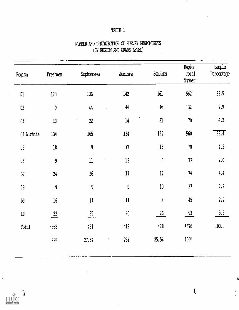
appropriate sample size for each region. Actual region totals and the

school class standing of the respondents are shown in Table 1. Hance,

the sample is a randomly selected groLp of high school respondents based

on relative population density. The sample of 1676 usable cases, resulted

Lsau inability to obtain permission to interview in two schools. The

data were collected during spring semester 1974.

Responses were then alalyzed for differences between those who had

had alcohol to drink within the last thirty days (alcohol involved) and

those who had not (non-involved) Those defined as non-involved included

those who had never drunk alcohol as well as those defined as irfrequent

drinkers.3 The actual number of cases presented in each table varies

due to non-responses to that question.

The survey instrument was a modified versiOn of the youth survey

questionnaire developed by the P:acenix Alcohol Safety Action Project.4

Only selected items are presented in this paper, but the report is avail-

able flout the athor upon request.

.

TABLE 1

NUMER AND DISTRIBUTION OF SURVEY RESPCNDEMS

(BY REGION AND GRADE LEVEL)

Region Freshmen Sophomores Juniors Seniors

'Region

Total

%ter

Sample

Percentage

01 123 136 142 161 562 33.5

02 0 44 44 46 132 7.9

n3 13 22 14 21 70 4.2

04 Lchita 134 165 134 127 560 33.4

05 18 19 17 16 70 4.2

06 9 11 13 0 33 2.0

07 24 16 17 17 74 4.4

08 9 9 9 10 37 2.2

09 16 14 11 4 45 2.7

10 22 15. 20 26 93 5.5

Total 368 461 419 428 1676 100,0

22% 27.5% 25% 25.5% 1001.

6

4

Analysis

Data were analyzed by use of non-parametric statistics. For the most

part the chi-:square and same namographs, a visual difference proportions

tests, have been used.5

The statistic and designated levels of signi-

ficance are presented with supporting tables when results are presented.

The .05 significance level has been used to specify significant sta-

tistical findings.

RESULTS

The results of this survey are presented for Wichita yough and

Kansas youth (Wichita youth omitted). The results are further subclassi-

fied by the operational definitian of drinking status of the respondents. As a

reminder the "alcohol involved" youth were those who reported they had

consumed alcohol within the last month. "Non-Alcohol Involved" youth

included respondents who reported never consuming alcohol or no con-

sumption within the last month prior to the study.

Socio-Demcgraphic Characteristics

The characteristics of sex, age, income, race, and school class

are examined in this sectian to see if any differences or trends existed

between Wichita and the remainder of the state or between those classified

as alcohol involved versus those who were not.

Sex

This cross tabulation between sex and drinker classification for

Wichita and the remainder of the state j_s presented in Table 2.

TABLE 2

SEX OF RESPONDENTS BY SAMPLE GROUP AND ALCOHOL INVOLVEMENT

Wichita Kansas

AlcoholInvolved

Non-AlcoholInvolved

AlcoholInvolved

Non-AlcoholInvolved

Sex # % E # % E # %

Male 149 53 227 78 33 344 52 501 157 40 728

Female 134 47 291 157 67 314 48 549 235 60 840

TOtals 283 100 518 235 100 658 100 1050 392 100 1568

55% 45% 63% 37%

33% 67%

x2 = 1.96 with 1 d.f., N.S.

The data presented indicate no difference in the percentage of males

and females classified as alcbhol involved for i± Wichita-Kansas comr

parisons. The 53 percent male Wichita sample is matched by the 52 per-

cent Kansas sample. On the other hand there are sex differences in

percentages among the non-alcohol involved. Only 33 percent of the non-

alcohol involved respondents in Wichita were male and 40 percent of

the non-alcohol involved Kansas sample were male. Although a greater

percentage of females constitute the non-alcohol group w±thin eadh sample,

the difference between males and females was not statistically signi-

ficant.

The totals for Wichita and Kansas show that a greater proportion

of Kansas respondents, both male and female, were alcohol involved cam-

pared to Wichitarespondents (55%-63%), but there were no significant

differences in the sex distribution of the sample.

6

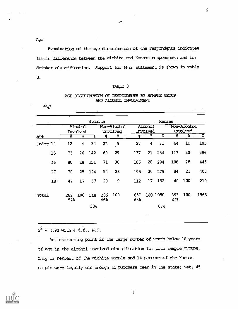
Examination of tha age distribution of the respondents indicates

little difference between the Wichita and Kansas respondents and for

drinker classification. Support for this statement is shown in Table

3.

..,7410./04

TAB,LE 3

AGE DISTRIBUTICN OF RESPCNDENTS BY SAMPLE GROUPAND ALCOHOL INVOLVEMENT

Wichita KansasAlcohol Non-Alcohol Alcohol Non-AlcoholInvolved Involved Involved Involved

Age # % E # % --IF % Z if % E

Under 14 12 4 34 22 ,9 27 4 71 44 11 105

15 73 26 142 69 29 137 21 254 117 30 396

16 80 28 151 71 30 186 28 294 108 28 445

17 70 25 124 54 23 195 30 279 84 21 403

18* 47 17 67 20 9 112 17 152 40 100 219

Tbtal 282 100 518 236 100 657 100 1050 393 100 156854% 46% 63% 37%

33% 67%

x2 = 2.92 with 4 d.f., N.S.

An interesting point is the large number of youth below 18 years

of age in the alcohol involved classification for both sample groups.

Only 13 percent of the Wichita sample and 14 percent of the Kansas

sample were legally old enough to purchase beer in the state; vet, 45

7

percent of the Wichita sample and 52 percent of the KansPs sample report

alcohol inyolvement prior to the time it is legal for them to purchase

alcohol. Further, the incidence of alcohol invi:flvement increases with

age for both sample groups; by age of 16, studellt-F were more likely to

report alcohol involvement; at age 18 or older, almost twice as many

students reported alcohol involvement. Eowever, the chi square sta-

tistic indicates there was no significant difference in the two groups

based on age of the students.

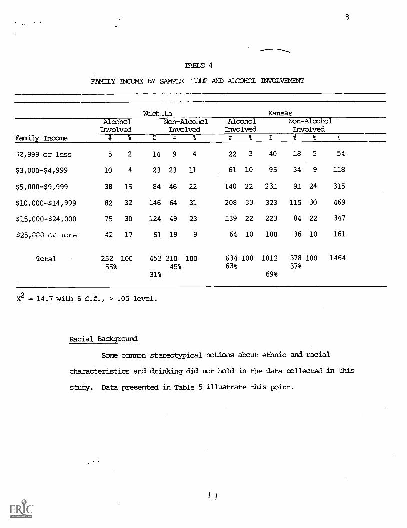
Family Income

Income data ara similar according to alcohol involvement for

both sample groups below the $15,000 level. Above $15,000 almost half

were alcohol involved in the Wichita sample but represented about one

third of the Kansas sample. Alcohol involvement was almost twice as

likely above the $25,000 income level for the Wichita sample. However,

independent of this trend of increasing alcohol involvement with

increasing inoome level for the Wichita sample, the total percentage of

alcohol involved respondents is les: than for out-state Kansas. The

figures and statistics can be seen in Table 4. There is a significant

difference in family income by residence found in these data.

8

TABLE 4

FAMILY INCOME BY SAMPLF 73UP AND ALCOHOL IWOLVEMENT

Wichta Kansas

Family Incare

AlcoholInvolved

Non-A1c0no1Involved

AlcoholInvolved

Non-AlcoholInvolved

# % Z i % # % E # % E

;2,999 or less 5 2 14 9 4 22 3 40 18 5 54

$3,000-$4,999 10 4 23 23 11 61 10 95 34 9 118

$5,000-$9,999 38 15 84 46 22 140 22 231 91 24 315

$10,000-$14,999 82 32 146 64 31 208 33 323 115 30 469

$15,000-$24,000 75 30 124 49 23 139 22 223 84 22 347

$25,000 or more 444,1 17 61 19 9 64 10 100 36 10 161

Total 252 100 452 210 100 634 100 1012 378 100 1464

55% 45% 63% 37%

31% 69%

X2 = 14.7 with 6 d.f., > .05 level.

Racial Background

Some common stereotypical notions about ethnic and racial

characteristics and drinking did not hold in the data collected in this

study. Data presented in Table 5 illustrate this point.

9MBLE 5

RACIAL BACKGROUND BY SAMPLE GROUP ANDALCOHOL INVOLVEMENT

Wichita Kansas

Race

AlcoholInvolved

Non-AlcoholInvolved

AlcoholInvolved

Non-Alcohollnvolved

# % E # % # % L # % E

AM Indian 6 2 13 7 3 29 4 40 11 3 53

Black 16 6 48 32 14 12 2 19 7 2 67

Mexican-Am. 4 1 9 5 2 12 2 20 8 2 29

White 238 87 411 17: 76 574 87 923 349 87 1334

Ott x 10 4 22 12 5 34 5 59 25 6 81

Total 274 100 503 299 100 661 100 1061 400 100 156455% 45% 62% 38%

32% 68%

= 49.12 with 4 d.f., < ,001 level.

There appears to be relatively little relationship between race and

involvement with alcohol in each sample. The Kansas sample had almost

identical proportions for all classifications, but there were two

marked differences in the Widhita sample. There were 11 percent more

whites classified as alcohol involved than non-alcohol involved and

there were 8 percent fewer blacks classified as involved than classi-

fied non-involved. Hence, notions of adult patterns of drinking

for same groups did not hold in these data. As with the income

variable, the Widhita sample Showed greater differences for alcohol

involvement according to racial badkground. Alcohol involvement appears

to be relatively uneffected by these variables in the Kansas sample.

There was a highly significant relationship in the computed chi

square. Most of the variance can be attributed to the over representation

of blacks in the Wichita sample. This difference of course reflects

the actual ri.itribution of black residents in the state, most are

urban residents.

10

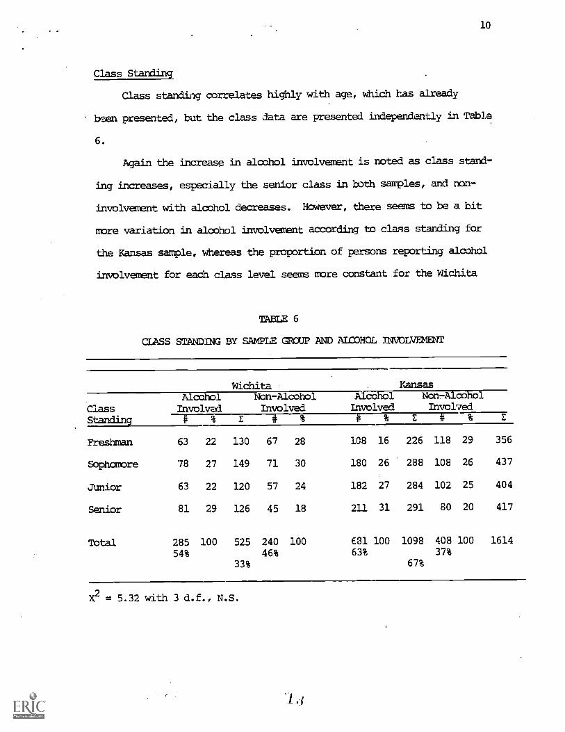
Class Standing

Class standing correlates highly with age, which has already

been presented, but the class data are presented independently in Table

6.

Again the increase in alcohol involvement is noted as class stand-

ing increases, especially the senior class in both samples, and non-

involvement with alcohol decreases. However, there seems to be a bit

more variation in alcohol involvement according to class standing for

the Kansas sample, whereas the proportion of persons reporting alcohol

involvement for each class level seems more constant for the Wichita

MIME 6

CLASS STANDING BY SAMPLE GROUP AND ALCOHOL INVOLVEMENT

Wichita Kansas

Class

at..12gli-E9

AlcoholInvolved

Non-AlcoholInvolved

AlcoholInvolved

Non-AlcoholInvolved

z # % # % E # % E

Freshman 63 22 130 67 28 108 16 226 118 29 356

Sophomore 78 27 149 71 30 180 26 288 108 26 437

Junior 63 22 120 57 24 182 27 284 102 25 404

Senior 81 29 126 45 18 211 31 291 80 20 417

Total 285 100 525 240 100 631 100 1098 408 100 1614

54% 46% 63% 37%

33% 67%

X2 = 5.32 with 3 d.f., N.S.

11

sample. There was no significant difference in the sample distribution

based on sampling procedures. Of course this finding of non significance

whould be expected if the sampling procedure is appropriate.

Drinking and Driving Behavior

Questions 1ining drinking and driving have been considered in

the following section. These included quastions About driving after

drinking, amount willing to drink and still drive, perceptions of

driving ability after drinking, concerns about driving while intoxi-

cated, deterrents to driving while intoxicated and probability decisions

.about driving after becoming drunk at a party.

Driving After Drinking

Slightly over one-third of both samples said they "never" drive

after drinking but there were marked differences between the alcohol

involved and the non-alcohol involved respondents. -These data along

with the remaining responses are Shown in Table 7.

It can be seen that the alcohol involved were more willing to

drive in an emergency and have more confidence in ther driving Ability.

The "no difference" responses really say, "It nakes no difference

how mudh I drink, I always drive anyhow". Clearly there were signi-

ficant differences between those classified as alcohol involved and

those classified as non-involved. Also there were significant differ-

ences between the Wichita and the Kansas group, the patterns and trends

12

TABLE 7

DRIVING AFTER DRINKING BY SAMPLE GROUPAND ALCOHOL INVOLVEMENT

Wichita Kansas

DriveAfterDrinking

AlcoholInvolved

Non-AlcoholInvolved

AlcoholInvolved

Non-AlcoholInvolved

# % E # % # % E # % E

Never 73 26 172 99 44 188 28 408 220 56 580

EmergencyOnly 50 18 59 9 15 103 15 131 28 7 190

Drive "but notwhen drunk" 61 22 66 5 2 243 36 258 15 4 324

No Difference 16 6 17 1 0 55 8 59 4 1 76

Don't Drive 77 18 187 110 49 83 14 206 123 32 393

Total 277 100 501 224 100 672 100 1062 390 100 1563

55% 45% 63% 37%

32% 68%

x2 = 11.68 with 3 d.f., > .01 level. N = 1170

in driving after drinking were quite similar with the exception that a

greater percentage of the alcohol involved Kansas sample reported

"driving often after drinking but never when drunk", compared to the

Wichita group. The outstate group clearly drive after drinking in

higher percentages than the Wichita group. The difference was signi-

ficant at the .01 level for those who drive.

13

Driving While Intoxicated

TO dheck driving experiences after drinking too mudh, the students

were asked haw many times they had driven when they "were really pretty

drunk?" _Again the alcohol involved and non-alcohol involved classifi-

cations hold as the major differences. Greater percentages of the

alcohol involved in bath sample groups have drivsn more frequently when

intoxicated. (See.data in Table 8).

TABLE 8

FREQQENCY OF DRIVING WHILE INTOXICATED BYSAMPLE GROUP AND ALCOHOL INVOLVEMENT

Wichita Kansas

Alcohol Non-Alcohol Alcohol Non-Alcohol

Involved involved Involved Involved

Times # % E # % # % Z # % Z

Never 154 56 314 160 69 349 52 676 327 81 990

1 - 2 61 22 69 8 3 178 26 192 14 4 261

3 - 5 11 4 11 0 0 43 6 46 3 1 57

6 - 10 7 3 7 0 0 18 3 19 1 0 26

Over 10 9 3 9 0 0 47 7 47 0 0 56

Don't Drive 34 12 98 64 28 38 6 95 57 14 .193

Total 276 100 508 232 100 673 100 1075 402 100 1583

54% 46% 63% 37%

32% 68%

X2 = 12.13 with 4 d.f., > .02 level. N = 1390.

The data indicate a slight tendency for more frequent drunk driving

by the Kansas alcohol involved group than the Widhita group. The

difference was substantiated by the .02 level significant dhi square

computed.

Amount Willing to Drink and Drive

"Haw much is the most you will drink and continue to drive?" was

asked to ascertain the students' judgement regarding how much alcohol

is perceived to be required to reduce driving ability after drinking.

The data again show the willingness of greater proportions of the

alcohol involved respondents, in both samples, to drive after drinking

larger amounts of alcohol. The response pattern NW quite similar for

the alcohol involved segment of each sample group, but there was no

significant difference between the Wichita and the outstate sample.

The trend is clearly related to the definition of alcohol involved

students, not to residence by sample.

TABLE 9

AMOUNT WIILMG TO DRINK AND DRIVE BY SAMPLEGROUP AND ALCOHOL INVOLVEMENT

Wichita.

AlcoholInvolved

Kansas

Non-AlcOholInvolved

Drinks

AlcoholInvolved

Non-Alcohor--Invo1ve0.

# % E # # % E # % E

1 - 0 57 21 160 103 45 146 22 384 238 60 544

2 38 14 48 10 4 81 12 108 27 7 156

3 29 10 38 9 4 75 11 94 19 5 132

4 22 8 25 3 1 54 8 62 8 2 87

5 18 7 20 2 1 61 9 63 2 .5 83

6 16 6 16 0 0 69 10 71 2 .5 87

7 - 9 16 6 20 4 1 46 6 48 2 .5 68

10 or more 17 6 17 0 0 66 10 71 5 1 88

Don't Drive 62 22 162 100 43 72 11 165 93 23 327

Total 275 100 506 231 100 670 100 1062 396 100 157254% 45% 63% 37%

32% 68%

x2 = 8.25 with 7 d.f., N.S. N = 1245

15

Driving Ability When Drunk

The students were asked to rate their driving ability while

under the influence of alcohol compared to when they had not been drink-

ing. Trends were similar in both sample groups but major differences

in perception can be seen between the alcohol involved and the non-

alcohol involved. Data presented in Table 10 indicate that a perception

exists that alcohol improved or at least does not negatively influence

TABLE 10

DRIVING ABILITY WHEN DRUNK BY SAMPLEGROUP AND AICOHOL INVOLVEMENT

Wichita Kansas

Ability

AlcoholInvolved

NOn-AlcoholInvolved

AlcoholInvolved

Non-AlcoholInvolved

# % E # % # % E # % E

Mud' better 10 4 11 1 0 20 3 26 6 2 37

Little better 15 5 15 0 0 28 4 30 2 0 45

Same 51 18 59 7 3 172 26 196 24 6 254

Little worse 76 27 90 14 6 193 29 209 16 4 299

Mich worse 18 6 19 1 0 42 6 49 7 2 68

Never drinkand drive 33 12 138 105 46 138 21 381 243 62 519

Don't Drive 74 18 177 103 45 76 11 170 94 24 347

Total 277 100 508 231 100 669 100 1061 392 100 156954% 46% 63% 37%

32% 68%

X2 = 5.09 with 5 d.f., N.S. n = 1222

driving ability is held primarily by the alcohol involved groups and

not shared by the non-alcohol involved group. The latter group, of

course, has had much less direct personal experience involving driving

after drinking. Most of the non-involved don't drive or do not drive

at all after drinking (Wichita, 91%; Kansas, 86%). It seems quite

likely, however, that most students responded to this question from

a general attitude rather than personal experience. Only 40 percent

of the Wichita alcohol involved sample and 32 percent of the Kansas

sample reported that they did not drive or did not drive after drinking

for this question. Other data, showing responses to the direct question

regarding dzinking after driving, indicated that 54 percent of the

Wichita alcohol involved group and 41 percent of the Kansas group

reported that they did not drive or did not drive after drinking.

In general, few respondents felt that alcohol improved their

driving ability but on the other hand, only a small percentage felt

that alcohol made their driving ability much worse, independent of

classification regarding alcohol involverent. Most respondents felt

that alcohol only made their driving ability a "little tiorse" or had

no effect. This perception was not significantly related to sample place

17

of residence as evidenced by the non-significant chi square.

Concern For Consequences of Driving While Intoxicated

The majority of respondents in each sample group, independent of

alcohol involvement, reported that the consequence of driving while

intoxicated that concerned them most was possible injury to others.

This concern was reported by a larger proportion of the Kansas sample

than the Wichita sample. The percentage figure for this response was

larger for the alcohol involved than non-alcohol involved in each

sample group, but this comparison is not totally accurate due to the

relatively larger percentage of non-alcohol involved respondents who

reported that they don't drive. (See data in Table 11.)

TABLE 11

CONCERN FOR CONSEQUENCES OF DRIVING WHILE INTOXICATEDBY SAMPLE GROUP AND ALCOHOL INVOLVEMENT

Wichita Kansas

AlcoholInvolved

NOn7AlcOholInvolved

AlcbholInvolved

Non-AlcOholInvolved

Cbncern # % E # % # % E # % E

Legal PrOblems 31 11 41 10 4 63 9 88 25 6 129

WteckInsurance 10 4 13 3 1 23 3 33 10 3 46

Injury to Self 14 5 23 9 4 32 5 54 22 6 77

Injury toOthers 148 53 239 91 39 438 65 662 224 56 901

Other 10 3 23 13 6 43 6 70 27 7 93

Don't Drive 63 22 164 101 43 53 8 140 87 22 304

MUltipleResponse 5 2 12 7 3 22 4 25 3 0 37

Total. 281 100 515 234 100 674 100 1072 398 100 1587

55% 45% 63% 37%

32% 68%

18

Of those who drive concern for injury to others far outweighed

concern over self-injury and all other concerns combined. The conse-

quence of legal problems was a distant second.00ncern for the alcohol

involved in both groups. The chi square test for sample differences

between the Wichita and the outstate sample produced a nan significant

result. Most of the variance in this variable can be attributed to

alcohol involvement not place of residence.

Students also were asked what would keep them from drinking too

much if they were at a party and knew they had to drive home. A

summary table has not been presented since responses were quite similar

to the pattern in Table 11. The majority of respondents indicated "fear

of accident" as the major deterrent factor. Another factor, a "disap-

proving date" was noted as a deterrent by 12 percent of the Wichita

sample and by 19 percent of the Kansas sample. Police and friends

had relrtively little influence (4% friends, 4% police, in Wichita;

and, friends 4% and police 9% in Kansas) as deterrents. Proportional

differences existed according to alcohol involvement classification.

Police were seen as a greater deterrent by the alcohol involved (7%

to 1% in Wichita and 12% to 4% in Kansas) with friends disapproval

slightly more inpartant as a deterrent factor for the non-aloohol

involved (Wichita 5% NA/I to 3% A/I and 5% NA/I to 4% A/I in Kansas).

Hence, same deterrent factors could be noted but perceived accident

possibilities were the most important factor in both samples.

19

Action After Becoming Drunk at a Party

Respondents were aSked what their action would be if: male,

and driver with a date and had too much to drink; or if female; with

date who was the driver, and date had too mudh to drink. The results

are presented in Table 12. The chi square statistics for this table

were computed by both sample residence and status. of alcohol involve-

ment. The data.were further separated by sex, hence there are two.'

statistics, one for-males and one for females

TABIE 12

ACTION MIER BECOMING DRUNK BY SAMPLE GROUP, ALCOHOLINVOLVEKENT AND SEX (PERCENTAGE OF RESPCNDENTS)

Wichita Ransas

Action

Alcoholinvolved

Non7AlcoholInvolved

AlcoholInvolved

Nen-AlcoholInvolved

Male Fenale Male Female Male Female Male Female

Drive Myself 20 59 8 35 24 59 9 49

Let (him-her)DriVe 59 8 59 8 60 13 62 3

Get a Friend 9 26 15 33 9 22 14 31

Call Taxi 9 3 12 13 4 2 13 7

Call Parents 2 2 4 16 0 2 2 10

Hitch Hike 1 2 2 0 3 2 0 0

Tbtal 100% 100% 100% 100% 100% 100% 100% 100%

X2 = 9.13 with 5 d.f., N.S. MaleX2 = 24.48 with 5 d.f., > .001 Female

20

The data presented in Table 12 show that general concensus existed

between males and females in both sample groups. Males %ere willing

to let their dates drive and their dates were willing to drive. Females

were more willing to drive themself or to ask a friend to drive. Males

seemed to rely more on their dates. The chi square result was not

significant when males were examined by rer4dence, alcohol invol'vement

and statenents of what they would do if they found they had drunk too

much at a party.

Alcohol involved nales in both sample groups were relativelylisaLe

willing to drive themselves than their non-alcohol involved counterparts.

Similarly, non-alcohol involved females %ere more willing to ask a

friend to drive rather than allow their date to drive when leaving

the party. It would seem that alcohol involved respondents in both

samples felt nom confident about their driving ability even after

drinking too much than non-alcohol involved respondents. These results

were consistent with results to the previous question regarding the

influence of alcohol on driving ability. Females significantly

differed in their responses as to what they would do if after driving

to a party they had drunk too much. For the most part they wouldn't

allow their date to drive the car.

Chances of an Accident

Students were asked to provide their perceptions of "the chances

of being involved in an autcrobile accident, if driving after drinking

too much". The findings in Table 13 show that the majority of all

respondentri, independent of sample group and alcohol involvement,

truncated that the chances of an auto acciamtwere high or very high

if driving after drinking too much. 'However, the percentage of res-

ponses for both the alcohol involved and non-alcohol involved for

the Wichita sample was greater than for the Kansas sample. In addition,

Z .1

21

more non-alcohol involved respondents felt that the dhances of an

accident were greazer than did the alcohol involved respondents in each

sample group. This general response pattern is quite consistent with

responses to the questions about consequences and deterrents regarding

driving after drinking too much.

MBLE 13

FERZEPISON CP CM= OF mtworpazNT IN AUTOACCIDENT AFTER DRINKING TOO MUCH BY SAMPLE

GIMP AND ALL:OHM4 INVOLVEMENT

Wichita Kansas

Chances

AlcoholInvolved

Non-AlcobolInvolved

AlcoholInvolved

Non-AlcoholInvolved

# % Z # % # %

Very High 81 29 190, 109 46 154 24 317 153 38 508

High 124 44 211 87 36 263 19 435 172 42 646

About Even 64 23 101 37 16 214 32 290 76 19 391

Low 10 3 16 6 2 27 4 32 5 1 48

Very Low 3 1 .3 0 0 12 1 12 0 0 15

Total 282 100 521 239 100 680 100 1086 406 100 160754% 46% 63% 37%

32% 68%

x2 = 16.76 with 4 d.f., > .01 level.

The computed chi sgaare was significant at the .01 level indicating

a difference in perceptions between the Wichita and outstate samples.

The Wichita sample saw higher probabilities of being involved in an

accident after drinking too much and driving. In both samples the

non-alcohol involved perceived higher probabilities of accidents than

was the case for the alcohol involved without ret.7ard for residence.

22

Discussion and Conclusions

TO obtain information about the drinking/driving attitudes,

behaviors and concerns of youth, a statewide survey was conducted in

1974. Respondents to the survey consisted of a proportional random

sample of youth in the state based on population density of the eleven

designated multi-county regions of Kansas.

Analysis of the data consisted of a comparison of responses of

youth from Wichita and youth from out-state Kansas. Each sample group

was further sub-divided into alcohol involved and non-alcohol iavolved

groups for within - and between-sample comparisons. Designation of

alcohol involved status was based on students' self-reparted consumption

of alcohol within the thirty days preceding the survey.

The Wichita and Kansas samples of respondents obtained were similar

in terms of the characteristics of class standing and age but family

income, and race differed significantly. in addition a.larger proportion of

the Kansas sample was alcohol involved compared to the Wichita sample,

63 percent to 54 percent. A notable finding for both samples was the

high percentage of alcohol involved respondents compared to the

percentage legallv able to purchase alcohol in the state. Only about

13 percent of each sub sample was old enough to legally purchase

alcohol (18 years for 3.2% beer), yet 45 percent of the Wichita sample

and 52 percent of the.Ransas sample below eighteen years of age were

alcohol involved by definition. Alcohol involvement tended to

increase with grade level in both samples and with increasing family

inoame, however, this latter trend evened out above the $15,000 annual

income category for the Kansas sample.

23

Data presented elsewhere, but relevant to this analysis indicate,

compared to the Wichita sample, a largerpercentage of the Kansas sample

held a valid driver's license/Permit, owned their own auto and had

received three or more moving traffic citations. These same t7.-ends

existed for the alcohol involved in each sample.

Thus, a larger percentage of the out-state Kansas youth and the

alcohol involved youth in eaCh sample more frequently drank alcohol,

were legally Able to (operate an auto, owned their own auto and received

traffic tidkets more frequently and had more multiple or repeat vio-

latins for moving offenses.

The drinking patterns of the alcohol involved respondents in

Loth samples were similar in that beer was the preferred alcOholic

beverage and alcohol was typically consumed on one day eadh week.

Whereas'a larger percentage of the Wichita alcohol involved group drank

one-ti-two drinks on an average drinking day, a larger percentage of

the Kansas sample drank three or more drinks. Another distinction between

these two gxtups was that 24 percent of the Kansas alcohol involved

group did most of their drinking while driving around, compared to

About 10 percent of tL., Widhita group. A relatively large proportion

of the alcohol involved in eadh sample also preferred to drink most

often at parties whith also presumably involved automobile transpor-

tation.

Higher percentages of the Kansas sample drank alcohol, drank

larger amounts when they did drink, and significantly larger per-

centages (24% Kansas, 10% Wichita)did most of their drinking while

driving around. There was a significant difference in willingness to

drive after drinking with the Kansas sample more willing to drive after

drinking. The Kansas samole also had driven while intoxicated more

often than the Wichita grcup. Seven percent of the Kansas sample

ported they had done so 10 or more times at the time of the study.

There was no significant statistic relating the amount respondents

were willing to drink and then drive. Most respondents felt that alcohol

consuntotion either had no effect on their driving or, at most, made

their driving ability "a little worse". Only the alcohol involved

respondents felt that their driving Ahility was improved after consuming

alcohol. More of.the Kansas alcohol involved sample reported driving

after &inking and driving when drunk more often than their Wichita

counterparts (significant .05 level).

The great majority of all respondents considered the chances of

involvement in an auto accident:when driving after drinking to be high

or very high:and their greatest OMMEMI was the consequence of possible

injury to others. Althou#I these feelings were shared by most

respondents, they wete held by a greater percentage of the non-alcohol

involved than alcohol involved respondents. The residence difference

was not significant.

An interesting sex diffenaloa was noted in what respondents would

do if they became drunk at a party. The alcohol involved males were

more willing to go ahead and drive (about 23%) than the non alcohol

involved males (about 9%). HOwever, females in all classifications

were more willing to drive after becoming druhk at a party (59% alcohol

involved females, 45% non-aloohol involvad). Conversely the males who

become drunk would allow their date to drive (60%), the females generally

would act (8%). There was a significant difference for females

(.001 level) but the rale test was not significant.

25

The non-alcohol involved perceived a much higher possibility of

becoming involved in an auto accident than was the case for the alcohol

involved. The chi square test for difference by residence was signi-

ficant at the .01 level with the Wichita sample perceiving higher

risks.

In.summary, there were significant differences between the Wichita

and the outstate respondents. Five of the eight chi square tests

of behavioral and perceptual variables were significmat. The Wichita

sample was,less likely to drink and drive, drive after drinking too

mudh, females were less likely to drive themself after drinking too

-much and perceived higher prohAhilities of becoming involved in an

auto accident after drinking too mudh.

Footnotes

1. Wilcox, Leslie D., et. al., Social Indicators and SocietalMonitoring, An Amlotated Bibliography, Jossey-Bass, Inc., ?ublishers,San Francisco, Ca., 1972.

2. Hansen, Morris, H., et. al., Sample Survey Methods and Theory,

John Wiley and Sons, Inc., New York, N.Y., 1953.

3. Communications Strategies on Alcohol and Highway Safety, Vblume II -High School Youth, February, 1975, Department of Transportation.

4. Unpublished report of the Phoenix Alcohol Safety Action Program,Phoenix, Arizona, 1974.

5. Leonard, Wilbert, M. II, Basic Social Statistics, West Publishing

Co., St. Paul, Minn., 1976.