document resume ed 193 313 tm 800 628 institution …document resume ed 193 313 tm 800 628 author...
TRANSCRIPT
DOCUMENT RESUME
ED 193 313 TM 800 628
AUTHOR Samejima, FumikoTITLE Research on the Multiple-Choice Test Item in Japan:
Toward the Validation cf Mathematical Models.INSTITUTION Office of Naval Research, san Francisco, Calif.$PONS AGENCY Office of Naval Research, Arlington, Va. Personnel
and Training Research Programs Office.fEPORT NO ONET-M3PUB DATE Apr 90CONTRACT N00014-77-C-0360NOTE 100p.
EDRS PPICE ME01/PC04 Plus Postage.DESCRIPTORS Foreign Countries: Latent Trait Theory: *Mathematical
Models: *Multiple Choice Tests: Psychometrics: *TestConstruction: Test Format: *Test Items: TestValidity
IDENTIFIEPS *Distracters (Tests) : Japan: K Index (Samejima) :Tailor Made Test: Three Parameter Model
ABSTRACTResearch related to the multiple choice test item is
reported, as it is conducted by educational technologists in Japan.Sato's number of hypothetical equivalent alternatives is introduced.The based idea behind this index is that the expected uncertainty ofthe m events, cr alternatives, be large and the number ofhypothetical, equivalent alternatives be close to m. A new index, K*,is proposed as a modification of m: it is a means of invalidating thethree-parameter logistic model for the multiple choice item. Shiba'sresearch on the measurement of vocabulary, which is based upon latenttrait theory, is introduced: this includes an eventual tailored testcr, vocabulary, utilizing information obtained from distracters aswell as correct answers. A new family of models for the multiplechoice item is proposed, formulating both the op6ratingcharacteristics of distracters and the effect of random guessing.(Author /GK)
************************************************************************ Reproductions supplied by EDRS are the best that can be made ** from the original document. ************************************************************************
APRIL 1980
SCIENTIFICMONOG
DEPARTMENT OF HEALTH.EDUCATION a WELFARENATIONAL INSTITUTE OF
EOUCATJON
THIS DOCUMENT HAS BEEN REPRO-DUCE D E xAC T Y AS RECEIVED FROM
OFT
PC OOR OROANQATIONol POINTS OF ,,,PEW OP OPINIONS
STATED 00 NOT NFCESSARitY PEPREIAL NATIONAL ,NSTITuTEOT-
EDUCATION POSITION OR POLICY
NRT M3
DEPARTMENT OF THE NAVY OFFICE OF NAVAL RESEARCH TOKYO
RESEARCH ON THE MULTIPLE - CHOICE TEST ITEM IN JAPAN:TOWARD THE VALIDATION OF MATHEMATICAL MODELS
Fumiko Samejima
IsF-afiaseeqe,
tts
iriPlAr:,t -',,.--.:.,, T ..,
,,,
W+.4
.,%.41.0,44.11,&
5
rt
I,
,A446.1.
;r1-4"
?s...raqif.se
".;
,e;
ONR Tokyo Scientific Monograph Series
ONRT M1 High Pressure Science and Technology in Japanby Earl F. Skelton, Naval Research Laboratory,Washington, D.C., July 1978
ONR-38 An Overview of Material Science and Engineeringin Japan by George Sandoz, ONR Branch Office,Chicago, Illinois, December 1977 (Reprinted in1980)
ONRT M2 Japanese Research Institutes Funded bx TheMinistry of Education, compiled by SeikohSakiyama, Office of Naval Research, Tokyo,January 1980
During the same period in which it was establishingONR Tokyo and the ONR Tokyo Scientific Monograph Series, theOffice of Naval Research supported and sponsored scientificliaison in Japan which led to monographs on selected segmentsof Japanese science. Those early monographs, which wereauthored in various elements of the ONR organization, arelisted here:
ONR-28 superconducting Technology in Japan by RichardG. Brandt, ONR Branch Office, Pasadena, California,June 1971
ONR-32 A Review of Some Ps chological Research in Japanby Morton A. Bettin, ONR Branc O ice, C icago,Illinois, November 1972
ONR-34 Computer Science in Japan by Richard L. Lau, ONRBranch Office, Pasadena, California, June 1973
ONR-36 Chemical Science in Japan by Arnet L. Powell, ONRBranch Office, Boston, Massachusetts, March 1973.
UNCLASSIFIEDSECURITY CLASSIFICATION OF THIS PAGE Man Data Ebar.41
REPORT DOCUMENTATION PAGE READ INSTRUCTIONSBEFORE COMPLETING FORK
L REPORT NUMBER
ONRT M3_
. GOVT ACCESSION NO. S. RECIPIENT'S CATALOG NUMBER
4. TITLE (and Sab$010
Research on the Multiple-Choice Test item inJapan: Toward the Validation of MathematicalModels
S. TYPE OF REPORT A PERIOD COVERED
6. PERFORMING ORG. REPORT NUMBER
7. AUTNOR(A)Dr. Fumiko SamejimaDepartment of PsychologyUniversity of TennesseeKnoxville, TN 37916
11. CONTRACT OR GRANT NUMBER(.)
NO0014-77-C-0360
9. PERFORMING ORGANIZATION NAME ANO AOORESSOffice of Naval ResearchScientific Liaison GroupAmerican EmbassyApp San' Francisco 96503
10. PROGRAM ELEMENT. PROJECT, TASK61%66 64R6 loon. NUMBERS
NR 150-402
t I. CONTROLLING OFFICE NAME AND ADDRESS
Office of Naval Research536 South Clark StreetChicago, IL 60605
12. REPORT OATS
April 198013. NUMBER OF PAGES
14. MONITORING AGENCY NAME A A000ESS(11 &Snoring hone Coninainnd Office)
Personnel and Training Research ProgramPsychological Sciences DivisionOffice of Naval ResearchArlington, VA 22217
IC SECURITY CLASS- (of Shia tenon)
UNCLASSIFIED
IS.. matvCATIO14/DOWNGRAOING
lc DISTRIBUTION STATEMENT (et Oda /Waft) 4
APPROVED FOR PUBLIC RELEASE: DISTRIBUTION UNLIMITED
17. DISTRIBUTION STATEMENT faiths &bonsai agitated in Mock 90, It Oillonnt neat FogNNO
IS. SUPPLEMENTARY NOTES
I. KEY SOROS (Cm01Avo on erne.. at* St "memoy and Meng* by Wear number)Educational test k* indexMultiple-choice test DistractersMathematical modelsVocabulary measurement
20. AsSTRACT (Continuo on ravers. nida 0 o ear, and idanilly by Moat ',abb.')
This monograph reports research, related to the multiple-choice test item,which is conducted by psychometricians and educational technologists in Japan.Sato's number of hypothetical equivalent alternatives is introduced. Theauthor proposes a new index, k*, which can be used, among other things, forinvalidating three-parameter models for the multiple-choice item. Shiba'sresearch on the measurement of vocabulary, which is based upon latent traittheory, includes an eventual tailored test on vocabulary, utilizing
DD I TRA,4'47, 103 EDITION of 1 NOV 1111 IS OBSOLETES/N 0 102..014.6601 I
UNCLASSIFIEDSECURITY CLASSIFICATION or THIS PAGE (What Data /noted)
AUG 4 1980
UNCLASSIFIEDTY Ct. 4SSIFIC4TION or THIS P4OC(Whon Dale Erteted)
20. Abstract (continued)
information obtained from distractors as well as correct answers. With thisresearch in mind, the author has developed basic ideas about a new family ofmodels for the multiple-choice item. These are based upon both theinformation given by distractors, and the correct answer and the noiseresulting from random guessing.
UNCLASSIFIEDSECURITY CLASSIFIC4TION OF 1141$ P4GE(Wheft Das Engem°
RESEARCH ON THE MULTIPLE-CHOICE TEST ITEM IN JAPAN:
TOWARD THE VALIDATION OF MATHEMATICAL MODELS
FUMIKO SAMEJIMA
DEPARTMENT OF PSYCHOLOGY
UNIVERSITY OF TENNESSEE
KNOXVILLE, TN 37916
APRIL 1980
Prepared under the contract number N00014-77-C-0360NR 150-402 with the
Personnel and Training Research ProgramsPsychological Sciences Division
Office of Naval Research
Approved for public release; distribution unlimited.Reproduction in whole or in part is permitted for
any purpose of the United States Government.
0
RESEARCH ON THE MULTIPLE - CHOICE TEST ITEM IN JAPAN:
TOWARD THE VALIDATION OF MATHEMATICAL MODELS
ABSTRACT
This monograph reports research, related to the multiple-choice test
item, which is conducted by psychometricians and educational technologists
in Japan. Sato's number of hypothetical equivalent alternatives is
introduced. The author proposes a new index, k*, which can be used, among
other things, for invalidating three-parameter models for the multiple-
choice item. Shiba's research on the measurement of vocabulary, which is
based upon latent trait theory, includes an eventual tailored test on
vocabulary, utilizing information obtained from distractors as well as
correct answers. With this research in mind, the author has developed
basic ideas about a new family of models for the multiple-choice item.
These are based upon both the information given by distractors, and the
correct answer and the noise resulting from random guessing.
V

PREFACE
In the summer of 1979, I spent a few weeks in Tokyo under the
sponsorship of the Office of Naval Research (ONR). This monograph is
based on conferences with researchers in Japan, in the areas of psycho-
metrics, educational measurement, and educational technologies, and on
research materials and technical literature collected during this trip.
thank Dr. Rudolph J. Marcus, Scientific Director, Hiss Eunice Mohri,
and other ONR/Tokyo staff members for providing me with office space
and services, taking we to JICST, and helping me in many other ways.
was invited to one of the bimonthly meetings of the Educational
Technology Group of the Institute of Electronics and Communication
Engineers in Japan, which was held at the Central Research Laboratories
of Nippon Electric Co., Ltd., on 23 July, 1979, and had an opportunity
to talk with the researchers who came to the meeting from many different
districts of Japan. The author is thankful to Dr. Takahiro Sato, the
representative of the Group, and other members for their kind cooperation
in collecting research materials and literature.
It was also a pleasure to have several conferences with Dr.
Sukeyori Shiba, Professor of Education at the University of Tokyo and an
old friend of mine, during my stay in Tokyo, and to get to know a large
scale research project on the measurement of vocabulary conducted by him
and his students. The author is thankful to him and his students for
making copies of their research materials and sending them to Knoxville,
Tennessee, after I returned.
vi
PREFACE (Continued)
Because of the shortage of time, the author could not see all
the people she had wanted to; among them are Professor Takeuchi of the
University of Tokyo and Dr. Akaike of the Institute If Mathematical
Statistics, who happened to be out of town during her stay in Tokyo.
The stimulation of these conversations, and of the research
materials and literature obtained in Tokyo, started new trains of
thought in the author's mind. Some of these concern the multiple-
choice item, which is the subject of this monograph. Others require
yet more work and further communication with Japanese colleagues. In
particular, the author feels it is worth trying to reanalyze the vocab-
ulary test data collected by Shiba and others, using theory and methods
which the author has developed and is going to develop.
The author is thankful to the Office of Naval Research for this
opportunity of visiting Tokyo, and hopes that the present report will
contribute to the development of mental test theory and science in
general.
viii
Fumiko Samejima

TABLE OF CONTENTS
I Introduction
Page
1
II Sato's Number of Hypothetical, Equivalent 5
Alternatives
III Information Given by Distractors in the 11Multiple-Choice Item and Random Guessing
IV Three-Parameter Models in Latent Trait 15
Theory and the Role of Item Distractors
V Index k* for Invalidating Three-Parameter 20Models
VI Shiba's Research on the Measurement of 32
Vocabulary
VII Use of Index k* when Distractors are in 48Full Work
VIII Proposal of a New Family of Models for the 55
Multiple-Choice Item
IX Discussion and Conclusions 68
References 70
Appendix I
Appendix II
Appendix III
ix
73
77
83
TKR I-1
I Introduction
There will not be any doubt in the mind of psychometricians
that good mental test items are informative items, which make a
great deal of contribution to the estimation of the examinee's
ability, and, therefore, uncover the individual differences among
the examinees accurately. In the history of mental test theory,
the multiple-choice item arrived later than the free-response
item, out of the necessity of administering group tests and of
scoring their results speedily and objectively, in the sense that
there is no need for our subjective judgment and evaluation in
scoring. Today, an enormous number of multiple-choice tests
are administered to youngsters, and their results have been used
in many important decision-making situations, such as guidance,
selection, classification, and so on. To construct good multiple-
choice test items and to develop good mental test theory which
deals with the multiple-choice item are, therefore, most important.
Since the multiple-choice item was introduced as a substitute
for the free-response item, it has been treated by mental test
theorists as something which is useful from the practical point of
view, but not quite as good as the free-response item. The three-
parameter logistic, or normal ogive, model, which is widely used
by psychologists and educational psychologists for the multiple-
choice item today, is nothing but a "blurred" image of the logistic,
or normal ogive, model for the free-response item. In other words,
there is nothing meaningful which is added to the original logistic,
or normal ogive, model, but there are additional noises caused
4.
-2- TICR T-2
by random guessing in the three-parameter logistic, or normal
ogive model.
We must stop and think, however, if the three-parameter
logistic, or normal ogive, model really fits psychological reality,
and if the multiple-choice test item cannot be more than a "blurred"
image of the free-response item. The author's answer to the first
question is negative, to the second positive. It is clear in the
author's mind that we need a better model than the three-parameter
logistic, or normal ogive, model for the multiple-choice item, and
that the multiple-choice item can provide us with a larger amount
of information which results in a more accurate ability estimation,
if we make use of the information given by its distractors, which
the free-response item does not have.
It was interesting to discover that, while very few researchers
in the United States have ever questioned the appropriateness of tbs._
three-parameter logistic, or normal ogive, model for the multiple-
choice item, and have tried to validade it for their research data,
the author's perception is shared by some Japanese researchers.
Some of these are members of a nation-wide research group called
the Educational Technology Group of the Institute of Electronics
and Communication Engineers in Japan. Most of the members of the
group are engineers in com-puter science, and some of them are
educational psychologists. Tatsuoka has reported their names
and research activities (Tatsuoka, 1979), which are represented
by such topics as the S-P table (Student-Problem table),
12
-3- TKR I-3
the number of hypothetical, equivalent alternatives*, interpretive
structural modeling based on graph theory, and so forth. Some of
their papers, which the author has had the opportunity of reading,
are listed in Appendix III. Their standpoint concerning the multiple-
choice item is based on information theory (e.g., Goldman, 1953),
considering that an item is a good one if its ezpected uncertainty
in the selection of an alternative is high. As the measure of
the quality of an item, the number of hypothetical, equivalent
alternatives (Sato, 1977) is used, which will be introduced in
Chapter 2. One impressive feature of the activities of this group
of researchers is that they do nct use computers mechanically,
as many other researchers do, but they give teachers the feedback
information about the test items constantly, and then they obtain
the teachers' feedback based on the content analysis of the items
in question, and so on. Another group is Shiba and his students of
the School of Education, University of Tokyo. They have spent the
past several years for developing vocabulary tests, which are
aimed at measuring vocabulary of subjects of a wide range of age,
collecting data, constructing an integrated vocabulary scale
(Shiba, 1978), and then constructing a tailored test out of these
vocabulary test items, using the information given by the distractors,
as well as the correct answers, for branching examinees (Shiba,
Noguchi and Haebara, 1978). The theory and method used for analyzing
their data are basically the same as those adopted in the research
in which the author was involved (Indow and Samejima, 1962, 1966).
*Tatusoka translated the original word as the effective (or equivalent)number of options, but the author uses this translation.
1 f--;
-4- TKR 1-4
The outline of the work accomplished by Shiba and others will be
given in Chapter 6.
With the research conducted by these people as incentives,
the author has integrated her own ideas about mathematical models
and the multiple-choice item. It resulted in proposing a method of
validating, or invalidating, the three-parameter logistic, or normal
ogive, model and the knowledge or random guessing principle, and
eventually proposing a new family of models for the multiple-choice
item, in which the information given by the distractors is fully
utilized.
1

-5- TKR 11-1
II Sato's Number of Hypothetical, Equivalent Alternatives
Let g (=1,2,...,n) be a multiple-choice test item. In the
present paper, however, this symbol g is omitted, whenever it is
clear that we deal with only one item. Let i (=1,2,...,m) be
an alternative, or an option, of the multiple-choice item g , and
pi be the probability with which the examinee selects the alternative
i . The entropy H is defined as the expectation of -log pi
such that
(2.1) H E pi log pi ,i=1
for the set of m alternatives of item g . It is obvious from
(2.1) that the entropy H is non-negative, and, if one of the m
alternatives is the sure event with unity as its probability, then
H = 0 . Sato's number of hypothetical, equivalent alternatives
k , is defined by
(2.2) k = 211
and is used as an index of the effectiveness of the set of m
alternatives for item g in the context of information theory.
Since the entropy H indicates the expected uncertainty of the
set of m events, or alternatives, the set of alternatives is more
informative for a greater value of k .
When the probability pi is replaced by the frequency ratio,
Pi , we can write for the estimate of the entropy such that
m(2.3) H = - E Pi log2 Pi ,
i=1
-6- TKR /1-2
and for the estimate of k we have
(2.4)2ii
We notice that we can obtain the number of hypothetical,
equivalent alternatives k without using the entropy, for we have
log2 p.m -p, m p
(2.5) k * 2H
= 2i=1
pi 1 - I n Pii -1
i=1 i*1
The quantity in the brackets of the last expression of (2.5) is
a kind of weighted geometric mean of pi . Equation (2.5) also
implies that we can use any base for log pi , instead of 2 .
For convenience, hereafter we shall use e as the base of log pi ,
and use H* instead of H such that
(2.6) H* - E pi logepi 0 ,
it
which equals zero when one of the alternatives is the sure event, and
(2.7) k eH*
1 ,
and simply write log pi instead of loge pi .
To find out the value of pi which maximizes H* , and hence
k , we define Q such that
(2.8) Q * E pi log pi Al: E pi-11 ,
i=1 i=1
where A is Lagrange's multiplier. Thus the partial derivative of
Q with respect to pi is given by
ag(2.9) - 1) .
Bpi pi
1.
-7- TKR II-3
Setting this derivative equal to zero, we obtain
(2.10) log pi = X - 1 ,
which is a constant regardless of the value of i . Since we have
(2.11)
we obtain
(2.12)
Z pi = 1 ,
i=1
p = lim .
Thus it is clear that H* , and hence k , is maximal when all the
m alternatives are equally probable, and we can write
(2.13) max (H*) = log m
and
(2.14) max (k) = m .
Since in the present situation the m events are alternatives,
the values of H* and k are affected by the difficulty level of
item g . Let R be the correct answer to item g , which is given
as one of its alternatives, and pR be the probability with which
the examinee selects the correct answer R . Figure 2-1 presents
the relationship between the probability pR and the number of
hypothetical, equivalent alternatives k . In this figure, the
area marked by slanted lines indicates the set of k's which are
less than max (kly and greater than max[l/pR, min (kIpR)], and
are considered to be reasonable values of k by Sato and others.

0.2
JIJit
0.2
R
0.8
0.0 0.5 1.0
PROBABILITY FOR CORRECT ANSWER
FIGURE 2-I
0.8
Relationship between the Probability with Which the CorrectAnswer R Is Selected and the Number of Hypothetical,
Equivalent Alternatives, for Five-Choice Items.

-9- TKR 11-5
In practice, Figure 2-1 is used by replacing the probability
pR by the proportion correct, FR , and the number of hypothetical,
equivalent alternatives, k , by its estimate i . It is well-known
that the frequency ratio is both the least squares solution and the
maximum likelihood estimator of the corresponding probability.
It is interesting to note that, in addition, it is the estimator
which minimizes the chi-square statistic. Let us define Q such
that
m m(2.15) Q = E [(NPI. Np
i)2/(Np
i)1 A( E p 1] ,
i=1 i=1
where N is the number of examinees and A is Lagrange's multiplier.
Then we have
(2.16) = ti[(1) P2)/p] + A . 0 ,ap i
and
(2.17)
Since
(2.18)
we obtain
(2.19)
3i = [1 (A/N)] -1/2 P1
1 =Epi=[1+(AAN-1/2E1).=[1 + (A/N)]-1/2
1=1 i=1
0 ,
and from this and (2.17) we can write
(2.20).131. Pi

-10- TKR 11-6
The translation, "the number of hypothetical, equivalent
alternatives," indicates the number of alternatives in the
hypothetical situation where the entropy H is provided by the
alternatives which are equivalent in the uncertainty of occurence.
Although it is not the direct translation of the original word,
it is used for k in the present paper, for it seems to the author
to be the best describing word of the original.
TKR III-1
III Information Given Distractors in the Multiple-Choice Itemand Random Guessing
Sato's number of hypothetical, equivalent alternatives has
been used mainly by the members of the Technical Group of Educational
Technologists in Japan (cf. Tatsuoka, 1979) for the purpose of
analyzing the effectiveness of alternatives in relation with
a relatively small group of examinees. The basic idea behind
this index is that the expected uncertainty of the m events, or
alternatives, be large, and, therefore, the number of hypothetical,
equivalent alternatives be close to m . We notice that:
(1) this concept is strongly population-oriented, unlike those
concepts in latent trait theory,
(2) it is assumed that each examinee tries to answer the item
seriously, without depending upon random guessing,
and,
(3) relative to the population of examinees, the existence of
too attractive a distractor is not desirable, since it
tends to reduce the value of k .
Thus as long as this index is used for the analysis of test items
which are given with careful guidance and supervision to samples
of examinees from a well-defined population, and the findings of
the analysis are not generalized across populations, it will serve
its purpose.
If we generalize this concept and the resultant findings
beyond these restrictions, however, we may be led to completely
r-)4
-12- TKR 111-2
false conclusions. To give an extreme example, suppose that none
of our examinees took the test seriously, and selected one of the
alternatives at random, for each item of the test. In such a case,
regardless of the difficulty level of the item, the number of
hypothetical, equivalent alternatives, k , will be very close to
m for every item! In spite of this superficial success, we have
obtained no information about the individual examinees' ability
levels as the result of testing.
It is also noted that, if the examinee's behavior follows
the knowledge or random guessing principle, i.e., he will answer
correctly if he knows the answer, or guess randomly otherwise, the
value of k tends to be large. In this case, too, our success
of obtaining a large k is only superficial and meaningless.
In addition to the above facts, it is obvious that the value
of the number of hypothetical, equivalent alternatives varies for
different populations, i.e., the same item may have a value of
k which is very close to m for one population of examinees,
and may have a very low value for another population. This may
be due to the difference in the mean ability levels of the two
populations, or to the different forms of two ability distributions,
or both. Thus while the index may be useful for a fixed population
of examinees and if we discuss "how good an item is" in relation to
that specific population, it cannot be considered as a parameter
of the item per se. This limitation of the usefulness of k
is of the same kind that is applicable for the reliability coefficient
of the test, i.e., in spite of most psychologists' belief that
9
-13- TKP. 111-3
the reliability coefficient is one of the most important and solid
properties of the test itself, it heavily depends upon the specific
population of examinees for which the test is administered, and
therefore, is a dead concept since the population-free test information
function is sufficient to serve the purpose (Samejima, 1977a).
As a whole, there is no single answer to the question: "Are
items which have high values of the number of hypothetical, equivalent
alternatives good items?" even if we control the testing situation
with respect to the purpose of testing, such as guidance, selection,
etc. This is true even if we restrict the populations of examinees,
and it is mainly because of the noise induced by random guessing.
That is to say, in a general situation of testing, it is hard for
us to determine whether we have accomplished the work by obtaining
a high value of k . In fact, the largest possible value of k
may imply no accomplishment at all, as we have seen in one of the
preceding paragraphs of the present chapter!
La spite of the above limitations, however, the introduction
of the number of hypothetical, equivalent alternatives and its use
by Sato and other researchers of the Technical Group of Educational
Technologists should be well credited, for their vision is
oriented toward the full use of the information given la all the
alternatives of the multiple-choice item. It seems that they
are quite successful in using the index in the small group situation,
such as school classes where instructions are well conveyed and
random guessing is extremely discouraged. This orientation is in
quite a contrast to the attitude of many researchers who are accustomed

-14- Tilt 111-4
to the blind use of the three-parameter logistic model for the
multiple-choice item, without ever stopping to think if the model
can be validated for their data.

-15- TKR
IV Three-Parameter Models in Latent Trait Theory and the Roleof Item Distractors
Let 9 be ability, or latent trait, that we intend to measure
with our.test. The three-parameter logistic model, or normal ogive
model, is based upon the knowledge or random guessing principle, i.e.,
the examinee either knows the answer or guesses randomly. Let T (e)
be the item characteristic function of item g , which is the
conditional probability with which the examinee answers item g
correctly, given 6 , in the free-response situation. This is given
by
-1/2ag(8-b
g)
e-u2
(4.1)/2
dug(6) - (210
in the normal ogive model, and
(4.2) f (e) = [1 + exp{-Dag(e-b
g)1]-1
in the logistic model, where a is the item discrimination parameter
and bg is the item difficulty parameter (Lord and Novick, 1968,
Chapter 16), and D in (4.2) is the scaling factor which assumes
1.7 (Birnbaum, 1968) when the logistic model is used as a substitute
for the normal ogive model.
The item characteristic function, P (8) , for the multiple-
choice item in the three-parameter normal ogive, or logistic, model
is defined by
(4.3) Pg(0) = 4'g (e} + 11-T
g(0)]e
g= c
g+ il-c
giT
g(0)
where Tg(8) is given by (4.1) or (4.2) and c
gis a constant which

-16-
.1==m1111
i
TKR IV-2
is called the guessing parameter, and equals 1 /mg , or 1/m .
It should be noted that, following these. models, there is
no information given by the alternatives other than the correct
answer, for all the responses to the wrong answers are the result
of random guessing. Should one of these models be valid for the
item in question, the multiple-choice item would be nothing but
a poor image of the binary, free-response item, which is contaminated
by the noise caused by random guessing.
Let j be an individual examinee, and uj be the binary
item score for the multiple-choice item g . The conditional
expectation and variance of the binary item score u , given e ,
can be written as
(4.4) Mule) Pg(0) = c (1-c)Tg(e) = (1/m)(1 (m-1)Tg(0)1,
where c is the simplification of c , and
(4.5) Var.(u18) = ((m-1)/m21[1-Tg(0)1(1-1-(m-1)Tg(e)1
Let uij
be the binary alternative score for the alternative i
obtained by the individual j , for the multiple-choice item g .
Thus we can write
(4.6) uRj = ui .
The conditional expectation and variance of the binary alternative
score u (OR) , given 0 , are given by
(4.7) E(uile) - (1/11)(1-7
-17-
and
(4.8) Var.(uile) = (1/m2)(1-Ts(8)][(m-1)+Vg(e)]
TKR IV-3
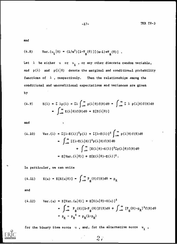
Let A be either u or ui , or any other discrete random variable,
and p(A) and p(A18) denote the marginal and conditional probability
functions of A , respectively. Then the relationships among the
conditional and unconditional expectations and variances are given
by
(4.9) E(X) =EXp(A) = EA fw p(A18)f(8)d8 = PiZAp(A18)f(6)d8
= E(Ale)f(e)de = E[Eais)]
and
(4.10) Var.(A) = E[A-E(A))2P(A) = E[A-E(A)]2 p(118)f(0)de
= E[A-E(A10)]2P(A10)f(0)d0
[E(118)-E(A)]2EP(X10)f(e)d0
= E[Var.(A18)] + E(E(Ale)-Emr.
In particular, we can write
(4.11) E(u) = ElE(u18)] = fce Pg(8)f(8)0 = pR
and
(4.12) Var.(u) = E[Var.(u10)] + E[E(ule)-E(u))2
= j'w Pg(8)(1-P (0))f(e)d0 + f [Pg(0)-pR
]2fuode
= PR PR2 PR(1-PR)
for the binary item score u , and, for the alternative score ui ,
9i.
-18- TKR IV-4
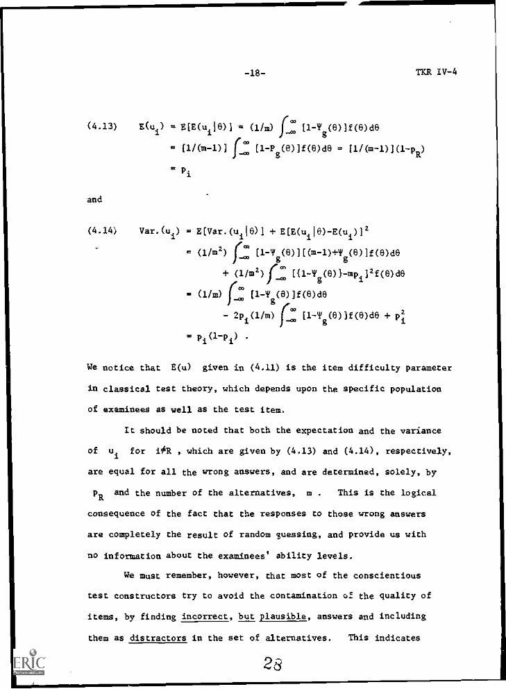
(4.13) Mui) = E[E(uile)) = (Um) re' fl-Tg(8)if(8)0
= [1/(m-1)] [. [1-Pg(e)]f(8)de t1 /(m-1)1(1-pR)
and
(4.14) Var.(ui) = E[Var.(ui(6)1 + E[E(uile)-E(ui)12
= (1/m2) jam, [l-tlig(0)][(111-1)+Tg(6)1f(8)de
+ (11m2)jrn ({1-Ts(8)}-mpi]2f(8)de
(1 /m) (1-Tg(8)]f(8)de
2pi(l/m) fcca 11-Tg(8))f(e)d8
= pi(1-pi) .
We notice that E(u) given in (4.11) is the item difficulty parameter
in classical test theory, which depends upon the specific population
of examinees as well as the test item.
It should be noted that both the expectation and the variance
of u for i #R , which are given by (4.13) and (4.14), respectively,
are equal for all the wrong answers, and are determined, solely, by
pR and the number of the alternatives, m . This is the logical
consequence of the fact that the responses to those wrong answers
are completely the result of random guessing, and provide us with
no information about the examinees' ability levels.
We must remember, however, that most of the conscientious
test constructors try to avoid the contamination of. the quality of
items, by finding incorrect, but plausible, answers and including
them as distractors in the set of alternatives. This indicates
28
-19-TIM/V-5
that the responses to these alternatives are not the result of random
guessing, and may contain useful information about the examinee's
ability level. The adoption of one of the three-parameter models
for such multiple-choice items is not justifiable, since in so doing
the researchers distort psychological reality and will produce
nothing but meaningless artifacts as the result of their research.
It is strange to the author that many researchers have ignored
the contradiction which was described in the preceding paragraphs,
and have applied the three-parameter models to their data for years,
which, obviously, are based on the tests containing many distractors.
As far as they continue repeating this mistake, their conscientiousness
as researchers has to be questioned.
-20-
V Index k* for Invalidating Three-Parameter Models
It has been pointed out in Chapter 3 that Sato's number of
hypothetical, equivalent alternatives takes on a high value, if
every examinee in the group has selected one of the a alternatives
at random. This fact implies that, although the index was introduced
for quite an opposite purpose, it may also be useful in detecting
the examinee's random guessing behavior in the multiple-choice
item.
To materialize the above, we need the following consideration.
When the examinee follows the knowledge or random guessing principle
and the item characteristic function assumes the three-parameter
logistic, or normal ogive, model, the index k is solely affected
by the probability with which the examinee knows the answer, as is
obvious from Figure 2-1 and (4.3) and (4.11). This fact provides
some inconvenience, however, for the probability of knowing the
answer heavily depends upon the specific population of examinees, in
addition to the item characteristic function of the item in ther.
*tree-response situation. It will be more convenient, therefore,
if we can modify Sato's index k in such a way that it is unaffected
by the ability distribution of a specific population of examinees,
and can be considered as a pure property of the item. With this
aim in mind, we shall introduce a new index in this chapter.
Let A be the event that the examinee does not know the
answer to item g , and consider the probability space which
consists of such a subpopulation of examinees. The conditional
probability, p(iii) , with which the examinee selects the alternative
30
-21- TKR V-2
i of item g in this conditional probability space is given by
(5.1) Pali)
' P I P ]-1i i R
V..01tT O-1at
Jri1/I
-1
where pit denotes the probability with which the examinee guesses
correctly for item g . The new index, k* is defined in terms
of these conditional probabilities, in such a way that
(5.2) k* = exp(- E P(1-1,1)*log P(iii)3 = [ n p(i1X)P(17)1-1 .
i=1 i=1
It is obvious that p(irk) for i#R is proportional to pi , for
every examinee in the population who has selected one of the wrong
answers does not know the answer, and, consequently, he is also
in the subpopulation I . On the other hand, examinees who have
selected the correct answer R are not necessarily in the
subpopulation A , so we can write
(5.3) Pa PR -
Note that, if the examinee's behavior follows the knowledge or random
guessing principle and the item characteristic function of the
multiple-choice item g is of one of the three-parameter models,
p* equals pi
for i#R , and, as the result, all the m p(ifI)'s
are equal and k* = m .
In practice, we need to use some estimates for p(iIA)'s
to obtain the estimate of k* . Since we have the frequency ratio,
Pi , for the estimate of pi for i#R , all we need to do is to

-22-TKR V -3
find out an appropriate estimate of pa . Let P* denote such
an estimate of p; , and Pt be such that
(5.4) p*
PR
i#R
i=R .
Then we can write for the estimate of pall) such that
(5.5) - p*[ r Pi] -1 .
We are to take the strategy of finding PR which makes k* maximal.
Define i* such that
a(5.6) fly = log i* = - E i(iII)
i*1m m
= -[ E P*] E P*log P* ( E P*)elog { E P*}] .
s*1 s i=1 i i i*1 i 8=1
Then the partial derivative of with respect to PR can be
written as
aft* 2 -2 m(5.7) 7r7,7 * Z P:1 [ E Ptelog Pt - ( E P*)log ,
R s=1 1.01 s=1 s
and, setting this equal to zero, we obtain
(5.8)
and then
(5.9)
log PI [ E Ps] -1 E Pielog Piaft
Pi ( E Ps j
P* = n Pi
siRR
i#R
Thus we can use (5.9) in (5.4), and therefore, obtain kill')
TKR V-4-23-
through (5.5). The estimate of the new index, k* , is given by
(5.10) i* * ex14- E [ fl f(i17)11(i111)]-1i*1
A necessary, though not sufficient, condition for one of the three-
parameter models to be valid is that k* should be equal to
within sampling fluctuations, regardless of the population of
examinees from which our sample happened to be selected. If this is
not the case, we must say that the three-parameter model does not
fit our item, i.e., the invalidation of the model.
Although the invalidation of the three-parameter logistic,
or normal ogive, model is easy, its validation is more difficult.
We recall that Sato's number of hypothetical, equivalent alternatives
is used as a measure of the desirability of the item for a specific
population of examinees. If all the distractors are equally probable
for a specific population, then the index k* will also equal m
in spite of the fact that the two cases are completely different
in nature. This problem can be solved by administering the same
test to a different group of examinees, which has a different
ability distribution from that of the first group. If the large
value of k* is due to the knowledge or random guessing principle,
then it will also be large for the second group of examinees because
of its population-free nature. On the other hand, if the large
value of k* is resulted from the optimal quality of the item for
the first group of examinees, then it will not be as large as that
for the second group, unless the operating characteristics of all
the distractors are identical.
-24-TKR V-5
It should be emphasized that k* takes on a large value even
if the knowledge or random guessing principle does not work behind
the examinee's behavior, but the item is "suitable" for the group
of examinees to which the test has been administered, in the same
sense that a high value of Sato's number of hypothetical, equivalent
alternatives is meant to indicate. This fact means that, when we
need to use only one set of data for validating, or invalidating,
the knowledge or random guessing principle and the three-parameter
logistic, or normal ogive, model, we must use, at least, one more
necessary condition for the principle to be valid. One such
necessary condition is that the sample means of ability 9 , or
of its estimate, of the subgroups of examinees who have selected
the wrong answers should be equal, within the range of sampling
fluctuations. Thus, if either the value of k* is substantially
less than m , or the sample means of ability 9 of such subgroups
of examinees are not close to each other, then we shall be able
to say that the knowledge or random guessing principle and the
three-parameter model are invalidated. On the other hand, if both
of the necessary conditions are satisfied with our data, we can say
there is no reason to reject the principle and the model.
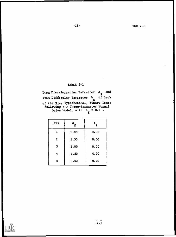
For the purpose of illustration, a set of simulated data was
calibrated, using the Monte Carlo method. In this set of data,
five hypothetical multiple-choice test items were assumed, sach
having five alternatives, A, B, C, D and E, with A always as the
correct answer. Each item is assumed to follow the three-parameter
normal ogive model, which is given by (4.1) and (4.3), with the
parameter values shown in Table 5-1. A group of five hundred
34
-25- TKR V-6
TABLE 5-1
Item Discrimination Parameter a and
Item Difficulty Parameter bg of Each
of the Five Hypothetical, Binary ItemsFollowing the Three-Parameter Normal
Ogive Model, with c = 0.2 .
Item ag
bg
1 1.00 0.00
2 1.50 0.00
3 2.00 0.00
4 2.50 0.00
5 3.50 0.00
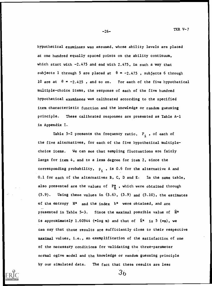
-26-TKR V-7
hypothetical examinees was assumed, whose ability levels are placed
at one hundred equally spaced points on the ability continuum,
which start with -2.475 and end with 2.475, in such a way that
subjects 1 through 5 are placed at 6 - -2.475 , subjects 6 through
10 are at e -2.425 , and so on. For each of the five hypothetical
multiple-choice items, the response of each of the five hundred
hypothetical examinees was calibrated according to the specified
item characteristic function and the knowledge or random guessing
principle. These calibrated responses are presented as Table A-1
in Appendix I.
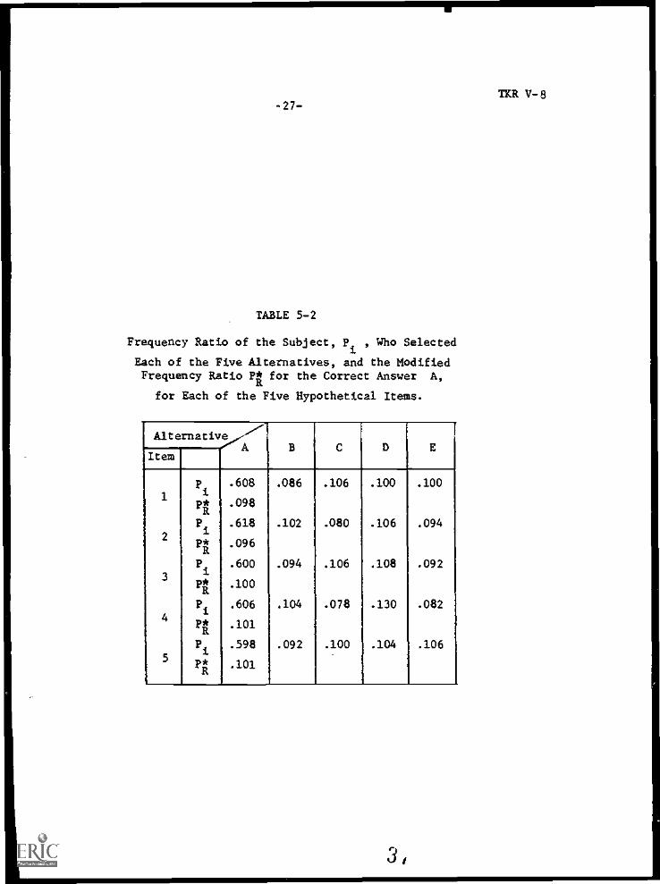
Table 5-2 presents the frequency ratio, Pi , of each of
the five alternatives, for each of the five hypothetical multiple-
choice items. We can see that sampling fluctuations are fairly
large for item 4, and to a less degree for item 2, since the
corresponding probability, pi , is 0.6 for the alternative A and
0.1 for each of the alternatives II, C, D and E. In the same table,
also presented are the values of P*R , which were obtained through
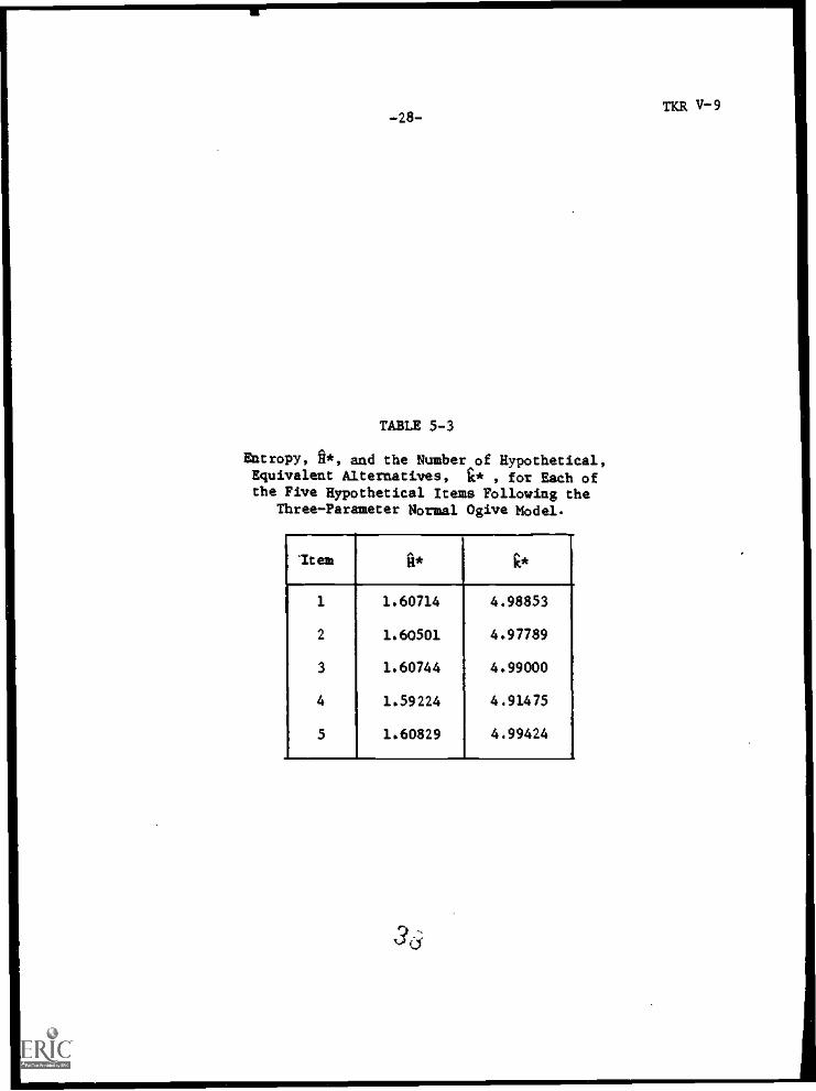
(5.9). Using these values in (5.6), (5.9) and (5.10), the estimates
of the entropy H* and the index k* were obtained, and are
presented in Table 5-3. Since the maximal possible value of fi*
is approximately 1.60944 ( -log m) and that of i* is 5 (*711), we
can say that these results are sufficiently close to their respective
maximal values, i.e., an exemplification of the satisfaction of one
of the necessary conditions for validating the three-parameter
normal ogive model and the knowledge or random guessing principle
by our simulated data. The fact that these results are less
36
1
-27-
TABLE 5-2
Frequency Ratio of the Subject, Pi , Who Selected
Each of the Five Alternatives, and the ModifiedFrequency Ratio P; for the Correct Answer A,
for Each of the Five Hypothetical Items.
Alternative.A B C D E
Item
1
2
3
4
5
pi
p*R
Pi
P*R
Pi
P*RPi
P*R
Pi
PR *
.608
.098
.618
.096
.600
.100
.606
.101
.598
.101
.086
.102
.094
.104
.092
.106
.080
.106
.078
.100
.100
.106
.108
.130
.104
.100
.094
.092
.082
.106
3
TKR V -8
-28-
TABLE 5-3
Entropy, fi*, and the Number of Hypothetical,Equivalent Alternatives, i* , for Each ofthe Five Hypothetical Items Following the
Three - Parameter Normal Ogive Model.
Item
....
fist kii
1
_
1.60714 4.98853
2 1.60501 4.97789
3 1.60744 4.99000
4 1.59224 4.91475
5 1.60829 4.99424
36
TKR V-9
-29-TKR V-10
satisfactory for item 4 and the same is true, to a lesser degree,
for item 2 must be due to the sampling fluctuations, which were
observed in Table 5-2.
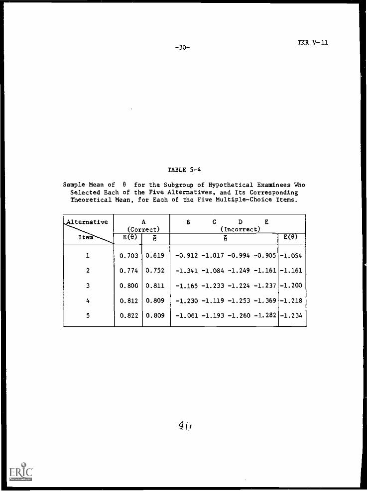
As another necessary condition for validating the three-
parameter normal ogive model and the knowledge or random guessing
principle, the mean of 8 for each of the five subgroups of
examinees, who selected different alternatives, was computed, for
each of the five multiple-choice items. Table 5-4 presents the
result of these means of 6 . In the same table, also presented
is the expectation of 8 for each of the five subgroups, using
the uniform ability distribution for the interval, [ -2.5, 2.5],
for each item, following the three-parameter normal ogive model
and the knowledge or random guessing principle. Since all the
responses to one of the four wrong answers of each item are nothing
but the result of random guessing, these alternatives are equivalent,
and have the same mean value of 8 . We can see that, for each
item, the mean of 6 for the correct answer and that of each
incorrect answer are substantially different, and they are close
enough to the respective theoretical means.
In practice,. there is no way to observe the examinee's 8
itself. We can use its maximum likelihood estimate, § , however,
and use it as the substitute in the above process, for example.
We must obtain a similar result as above, to validate the three-
parameter models and the knowledge or random guessing principle.
We notice that a similar result as the one in our example
3j
TKR V-11-30-
TABLE 5-4
Sample Mean of 8 for the Subgroup of Hypothetical Examinees WhoSelected Each of the Five Alternatives, and Its CorrespondingTheoretical Mean, for Each of the Five Multiple-Choice Items.
Alternative
Item
A(Correct)
B C D E(Incorrect)
E(8) ; ; E(8)
1 0.703 0.619 -0.912 -1.017 -0.994 -0.905 -1.054
2 0.774 0.752 -1.341 -1.084 -1.249 -1.161 -1.161
3 0.800 0.811 -1.165 -1.233 -1.224 -1.237 -1.200
4 0.812 0.809 -1.230 -1.119 -1.253 -1.369 -1.218
5 0.822 0.809 -1.061 -1.193 -1.260 -1.282 -1.234
4(1
-31-
can be obtained, if, incidentally, all the distractors require
TKR V -12
"on the average" approximately the same level of ability for the
examinee to be attracted to them, for our group of examinees.
This fact indicates that it is desirable to add more necessary
conditions to examine, such as the approximate equality of the
second moment of 8 , or § , that of the third moment, etc.,
for the subgroups of examinees who have selected the wrong answers.
Since these subgroups of examinees are "equivalent" in ability
distribution if the knowledge or random guessing principle and
the three-parameter model are valid, these higher moments should
be equal within sampling fluctuations, which it is highly unlikely
that all the subgroups of examinees who have been attracted to
separate distractors are equivalent in ability distribution. We
must avoid, however, using moments of too high degrees, for their
sampling fluctuations tend to be enormously great.
-32-TER VI -1
VI Shiba's Research on the Measurement of Vocabulary
In this chapter, we shall introduce a research on the
measurement of vocabulary, which was conducted by Shiba and others.
The author found it interesting, especially in the following aspects.
(1) The vocabulary tests they used are very well constructed,
choosing each alternative carefully.
(2) Subjects were selected from many different age groups.
(3) Unlike many researchers in the United States, they have
tried to make a full use of the distractors.
The battery of tests used for the construction of the
vocabulary scale consists of eleven tests, Al, A2, A3, A4, A5, A6,
Jl, J2, Sl, S2 and U . Each test contains thirty to fifty-eight
multiple - choice items, each having a set of five alternatives.
These tests differ in difficulty, and each of them is designed for a
different group of ages, ranging from six years of age to the ages of
college students. There are subsets of items included in two tests,
which are adjacent to each other in difficulty. For example,
items 37 through 56 of Test Jl are also items 1 through 20 of Test
J2. The number of examinees used for the vocabulary scale
construction varies between 412 sixth graders of elementary schools
for Test A5 and 924 second graders of senior high schools for Test
Sl. (cf. Shiba, 1978.)
The model adopted for the item characteristic function of
each vocabulary item is the logistic model, such that
(6.1) P (8) ft (1 + exp{-Da (13-1) )).]-1 ,
g g
4'
-33-TKR VI -2
where ag and bg are the item discriminationnd difficulty
parameters, respectively, and D a 1.7 . Note that Shiba did not
use the three-parameter logistic model, which is characterized by
(4.2) and (4.3). This is based on his belief that three-parameter
models are not applicable for well-developed multiple-choice items,
which he has formed through his many experiences in test construction
and research.
Each of the eleven tests was administered to a group of subjects
who belong to a single school year, except for college students.
Hereafter, for convenience, we shall use EL for elementary schools,
JH for junior high schools, SR for senior high schools, and CS for
colleges, and add the school year after each symbol. For instance,
by S82 we mean a group of subjects who are in the second year of
senior high schools. The correspondence of the subject groups and
the tests administered is summarized as follows:
Al for EL1 (650), A2 for EL2 (650), A3 for EL3 (546),
A4 for EL4 (617), A5 for EL5 (599), A6 for EL6 (412),
Jl for Mil (614), J2 for .1H2 (758), S1 for SH1 (924),
S2 for SH2 (759) and U for CS (740) ,
where the numbers in parentheses indicate respective numbers of
examinees. Note that JH3 and EH3 are not included in the data
which are the basis of the vocabulary scale construction.
The main steps for analyzing these data are the following.
[A] For each of the eleven groups of examinees, the ability
distribution is assumed to be the standard normal distribution.
[B] Assuming the normal ogive model, such that

-34-
) 2(6.2) P 0) - (27) "4 g g
e-1.1 /2
du
TKR VI-3
where ag and bg are the item discrimination and difficulty
parameters, respectively, and the local independence of the
item variables (Lord and Novick, 1968, Chapter 16), and also
that the regression of each item variable on ability 0 is
linear, the tetrachoric correlation coefficient is computed
for each and every pair of items.
[C] The principal factor solution of factor analysis is applied
for the correlation matrix thus obtained, using the largest
absolute value of the correlation coefficient in each row,
or column, as the communality. This step is also the process
of validating the uni-dimensionality of ability 0 . Figure
6-1 illustrates the resulting set of eigenvalues for Test Jl
which was administered to 614 first year junior high school
students. It turned out that the first eigenvalue is much
larger than all the other eigenvalues, and thus the uni-
dimensionality was confirmed. Hereafter, this first principal
factor is treated as 0 .
[D] From the result of factor analysis, the item parameters are
obtained. Let8
be the factor loading (e.g., Lawley and
Maxwell, 1971) of the first principal factor, or 6 , for item
g The item discrimination Parameter, ag , is obtained by
(6.3) a i p (1-p )-1/2
8 8 8 4

10.0
5.0
0.0
-3g-
1 2 3 4 5 6 7 8 9 10
ORDER IN MAGNITUDE
FIGURE 6-1
TKR VI-4
Eigenvalues of the Correlation Matrix of the Fifty-Five Itemsof Test 31, Ordered with Respect to Their Magnitudes.
-36- TKR VI-5
Let 0(u) denote the standard normal distribution function,
such that
(6.4) 0(u) = (270-1/21
e-t2/2
dt03
The item difficulty parameter, bg , is given by
(6.5) b * 0-1
(1-pgr
) p$ -1
where pgR is the probability with which the examinee answers
item g correctly. In practice, this is replaced by the
frequency ratio, PgR , to provide us with the estimate of
b .
g
[E] The eleven ability scales thus constructed are considered to
be on the same continuum, and they are integrated into a single
scale. This equating is made through the ten subsets of items,
each of which is shared by two adjacent tests. Let ag and
bg be the item parameters estimated from the result of the
first test, and a* and b* be those from the result of the
second test. Denoting the two ability scales by 9 and el, ,
respectively, we can write
(6.6) aS(s-b ) * a*& (e*-b*) ,
since the item characteristic functions, which follow the
normal ogive model, of the same item g on the two ability
scales must assume the same value for the corresponding values
of 8 and 8* . Thus the functional relationship between
4
-37-
6 and 6* is given by
(6.7) 0* = (a /a*)0 + (b*-(a&&/a*)b& ] ,
TKR VI -6
which is linear, and the two coefficients are obtained from
these four parameters. In practice, we obtain as many sets
of coefficients as the number of common items, and we need to
use some type of "average" of these coefficients for the scale
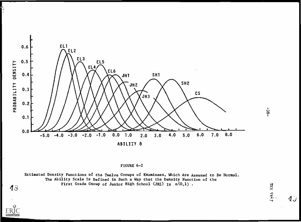
transformation. Figure 6-2 presents the ability distributions
of the eleven subject groups after such transformations were
made and the mean and the standard deviation of the distribution
of 31 are taken as the origin and the unit for the new,
integrated ability dimension.
IF] The item characteristic function of each item on the new,
integrated scale 0 is approximated by the logistic function,
which is given by (6.1).
(G] The maximum likelihood estimate, 6 , of each examinee's
ability is obtained through the equation
(6.8)n
a P (4.))
E a u
g g j g gj
(cLurniumm,1968),Ndlereo.&J
is the binary item score of
individual j for item g .
[HI The test information function of each test is obtained by
(6 . 9)
n1(6) = E I (8) ,
g
where I (e) is the item information function of item g such
4.
43
0.6-
0.5)-
0.4 -
0.3 -
0.2
0.1-
0.0
Ell
EL3 EEL5L4EL6
1
H 2
CS
-5.0 -4.0 -3.0 -2.0 -1.0 0.0 1.0 2.0 3.0 4.0 5.0 6.0 7.0 8.0
ABILITY 0
FIGURE 6-2
Estimated Density Functions of the Twelve Groups of Examinees, Which Are Assumed to Be Normal.The Ability Scale Is Defined in Such a Way that the Density Function of the
First Grade Group of Junior High School (JH1) Is n(0,1) .
co
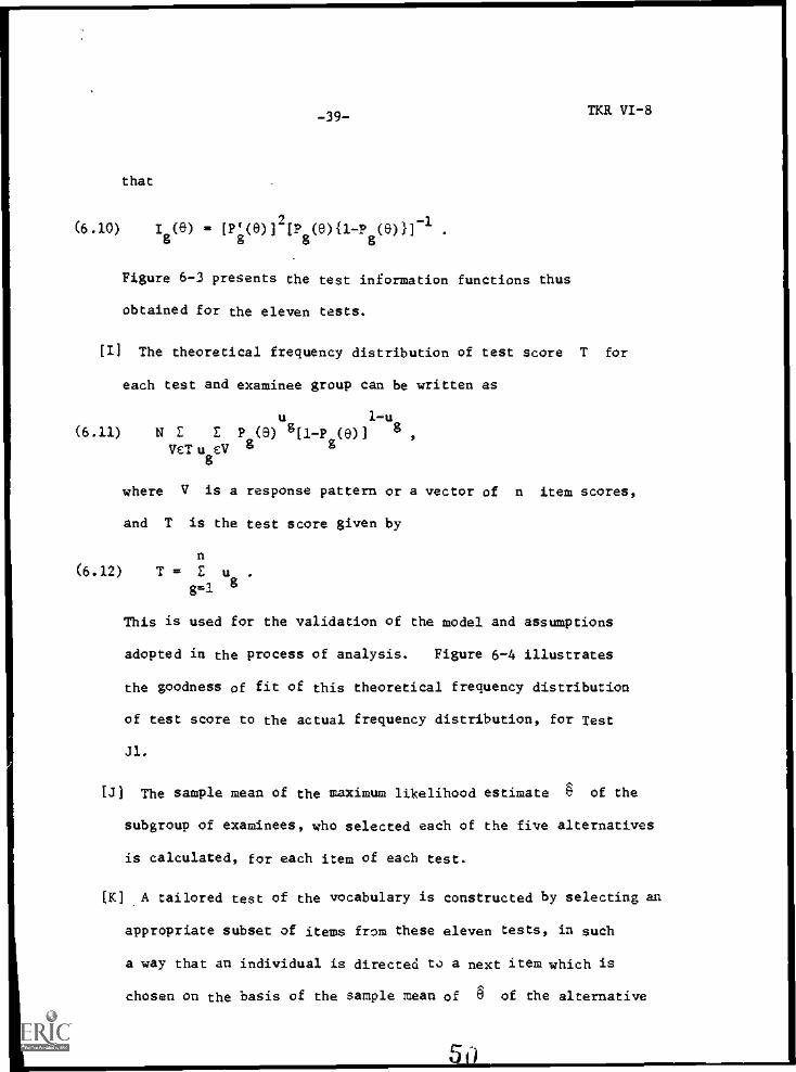
-39-
that
(6.10 (8) - (1"(e)]2
(e){1-P (On-1
8 8
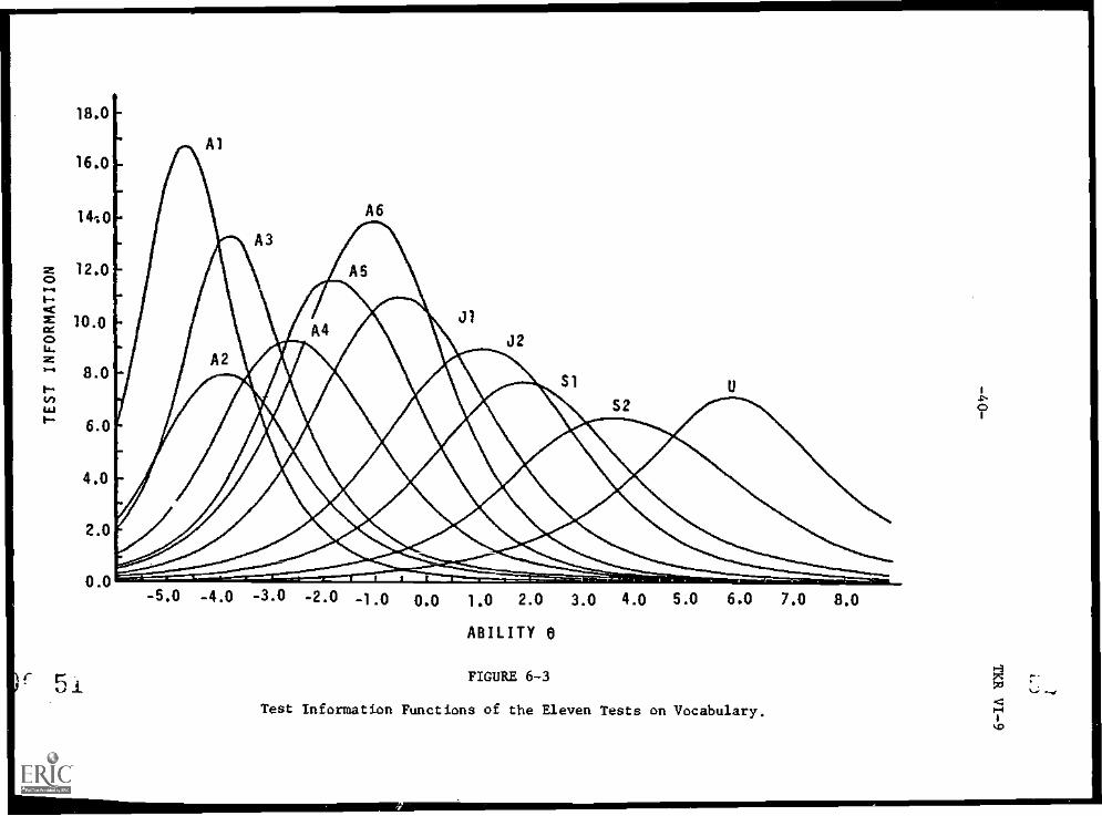
TKR VI -8
Figure 6-3 presents the test information functions thus
obtained for the eleven tests.
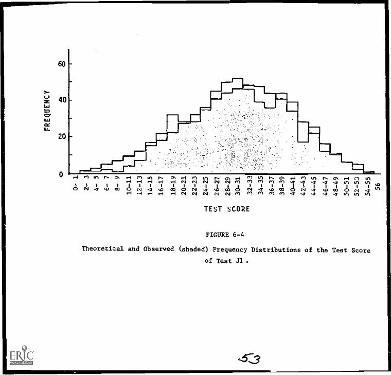
[I] The theoretical frequency distribution of test score T for
each test and examinee group can be written as
u 1-u(6.11) N E E P (9) g[1-P (0)] g
Vern8CV g
where V is a response pattern or a vector of n item scores,
and T is the test score given by
n(6.12) T E u .
g=-1 g
This is used for the validation of the model and assumptions
adopted in the process of analysis. Figure 6-4 illustrates
the goodness of fit of this theoretical frequency distribution
of test score to the actual frequency distribution, for Test
J1.
1J] The sample mean of the maximum likelihood estimate g of the
subgroup of examinees, who selected each of the five alternatives
is calculated, for each item of each test.
[K] A tailored test of the vocabulary is constructed by selecting an
appropriate subset of items from these eleven tests, in such
a way that an individual is directed to a next item which is
chosen on the basis of the sample mean of g of the alternative
51)
140
12.0
10.0
8.0
6.0
4.0
2.0
0.0
A6
J2
-5.0 -4.0 -3.0 -2.0 -1.0 0.0 1.0 2.0 3.0 4.0 5.0 6.0 7.0 8.0
ABILITY 6
FIGURE 6-3
Test Information Functions of the Eleven Tests on Vocabulary.
60
0
TEST SCORE
FIGURE 6-4
Theoretical and Observed (shaded) Frequency Distributions of the Test Score
of Test J1.
-42-
he has selected for the present item.
TKR VI-11
We have seen in the preceding paragraphs a brief sketch of
Shiba and others' work. It is unfortunate that the author cannot
convey the fine quality of the tests themselves to the reader, for
they are vocabulary tests and their translation from Japanese into
English would certainly destroy the nature of the tests. We can
see that the research has been conducted very conscientiously,
however, including several processes of validation, and has eventually
produced a widely applicable vocabulary scale and a tailored test.
In the latter result, although there is some room for improvement,
the use of distractors for "branching" subjects should be taken
as a stimulation to the researchers who are engaged in this area,
for it has seldom been seriously investigated by other researchers.
The research conducted by Shiba and others includes more
interesting data than were used in the vocabulary scale construction.
Table 6-1 presents a part of them, in which the frequency
distribution of the alternative selection and the mean of the
maximum likelihood estimate of ability for each alternative are
shown for nineteen items included in both Tests Jl and 32, and
administered to four different subject groups, ail, JH2(a), JH2(b)
and JR3. In the same table, also presented is the discrepancy
between the mean of ; for the correct answer and the lowest
mean ö for one of the four wrong answers, under the heading,
"largest discrepancy." The correct answers are always identified
as the ones which have the highest means of 0, except for the one
for item 8 administered to JH2(b), which is the second highest
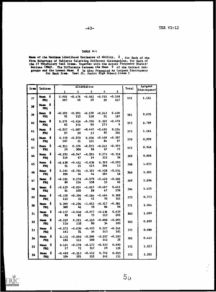
-43- 'Nit VI-12
TAKE 6-1
Mean of tba Maximum Likelihood Estimates of Ability, 6 for Each of theFive Subgroups of Subjects Selecting Different Alternatives, for Each oftba 19 Vocabulary Test Items, 'together with the Actual Ftequency Distri-butions (FRQ). The Difference between the Mesa 4 of the Correct Sub-groups and the Lowest Mean $ Is Also Pressured As Largest Discrepancy
for tech Irma. Test 31, Junior High School Grade 1
It's Indices
-
1
Alrernerive
2 3 4 5Total
LargestDiscrepancy
37
SS
39
40
41
42
43
44
0
46
47
48
49
SO
51
52
53
34
33
54
Mean 8
/IQ
Esse $FIQ
Mean 8FRQ
Mean I
FRQ
Mean $
rig
Mess 4FRQ
Mean 4
Fag
Mean 1
FRQ
Mean iFRQ
Mean 4
FRQ
Mean 4
TMMean 4
FRQ
Mean 8
FRQ
Mean $
Pig
Mean 8
FIQ
Mean I
FIQ
Mean i
FRQ
Wean $
FRQ
Mean $
FRQ
Mean 4
FRQ
0.401287
-0.192
91
0.07160
-0.55753
0.339247
-0.51226
-0.293119
-0.63851
0.444296
-0.26169
-0.12981
-0.339115
0.349308
-0.13789
-0.219116
-0.071163
0.132182
0.11427
-0.460104
-0.47650
-0.091115
-0.416141
-1.00720
-0.57021
0.376308
-0.54767
-0.41225
-0.74146
0.270224
-0.024100
-0.39031
-0.25646
-0.64082
0.291235
-0.03031
-0.060111
-0.27872
-0.113101
-0.48259
-0.270118
-0.33690
-0.44523
0.036121
-0.57298
-0.59514
-0.636123
-0.32544
-0.078158
-1.01358
-0.28442
-1.01535
-0.07775
-0.11080
-0.45334
-0.084100
-0.172317
-0.412115
- 0.750
59
-0.24351
0.310273
-0.45685
-0.43984
-0.24567
0.271333
0.395346
-0.428164
-0.42653
-0.46767
4-0.46470
-0.31786
-0.136113
-0.60834
0.527143
-0.037142
-0.53329
0.742141
-0.148117
0.400187
-0.4799
0.254
392
-0.38797
-0.39373
-0.31836
-0.59323
-0.53418
-0.10165
0.412258
0.309315
-0.36596
0.429201
-0.095100
-0.241181
-0.28326
0.6,0126
0.015111
572
562
573
573
570
572
569
568
568
569
564
573
571
560
565
572
561
'''
572
1.151
0.670
0.789
1.261
0.909
0,948
0.866
1.033
1.185
0.696
1.425
0.773
1.364
1.069
0.899
0.980
0.415
1.223
1.202
E479"T
Ziri
99e0
TECO
£11"0
69T'i
ZEV'T
SLT'T
09L"T
856'0
009"i
i6Z'T
168'0
69£'T
9£Z"T
OTZ"I
880"T
£80'1
861'1
---
SO
80
TO
60
Oh
et,
SO
094
50
60
60
60
90
80
tSt
T9t
80
00
SO
LL 81T 08 001 OL
LtZ"O 475E'T 681'0- 9E1"0 951'0
TOZ 81 ta 0 OZ tivl ii47"0- zi0.0- 270.0- m*0-
6 80T Z8 SL UT 150'0 TWO 181"0 951'0 LI8"0
511 081 91 tE 476
00'0 816'0 £10'0- 56'1'0 9LE"0
85 TZ it 6E/ 09 LLT"0 901"0 5E0'0 811"0 SWO
ZOZ 89 CC t, 9L
606'0 O5T"0 TWO 091'0- 8TI"0
£9 te OZ 6T 691 660'0- TWO 47E9'0- £51"0 86C0
4761 SE 61 91 96 95L"0 614'0- £81"0 ISCO- 050'0
TEZ 0 8£ S8 9S
1L8"0 980'0- 688'0- 191"0 Eet"O
OE OE vC ZOE Et 100'0- 'WO- 6I1"0- 491"0 9E1'0-
L 06 6Z SZ 80E
Zt0"0- 091'0- £91"0- TS1"0- 678'0
81 66Z 6L £Z 0£ 694760- C18"0 061'0- 6E1'0 tZT'O-
1£ I61 SI VS S9
tEZ"0 799"0 811'0- 01'0- 861"0
LE 947 ES ZTE OT
TZE"0- 1471"0 8t5"0- 16L"0 19T"0-
TS L9 89 VT LSZ TOZ0- 680'0- 844'0 9/7'0- 018'0
SSE tt 6T CI LZ 599"0 6T0"0- E11"0- O74"0- ES5"0-
VT CtZ 0 S6 19 98Z0- 208"0 60T"0 E£1"0- 115'0
99T OS 18 L6 SS 510"1 890'0- C80'0 981"0 'WO
TL t£ 6£ 6£ 691
8Z0"0 ZiE"0- 07'0- 511"0- 988'0
MU 0 usam
bu t u"14
hi ,
t uW NA
t usam
Did
9 um Did
@ 'as/ii
bid 9 Imit
bid
t %mom
aid
9 am bid
1 wok bid
9 milvii
b
t
bid
wyti
bid
g imm bid
9 two}
bu f useli
bid 9 vrm
bid t tweN
bid t mail
e
Du 12,441
bid
9 um
95
SS
45
CS
15
IS
OS
67
8,
tv
94
St
tt
Et
ZI/
It
07
6£
EIE
Lt
xouwayi3sT0 zsdayl
Isle/ s t E Z 1
a:41111=1v se3Tput Iran
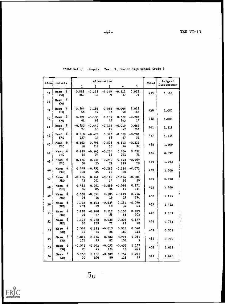
Z *PeID To0435 48tH infant 'Tr 2/01 :(P0/111? -) 1 -9 7101
-717-
-45-
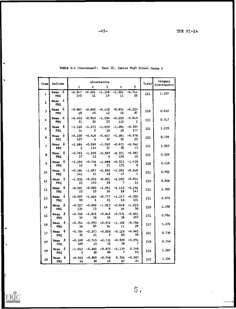
TABLE 6-1 (Continued): Test J2, Junior High School Grade 3
/tea Indices1
Alternative
2 3 4 5Total
LargestDiscrepancy
6
10
11
12
13
14
IS
16
17
IA
19
20I
Mean 8FRQ
Mean e
FRQ
Mean i
FRQ
Mean 8FRQ
Mean 4FRQ
Mean i
FRQ
Mean i
FRQ
Mean i
FRQ
Mean 6FRQ
Kean 8FRQ
Mean i
FRQ
Mean i
FIQ
Mean i
FRQ
Mean 6FRQ
Mean 8FRQ
Mean 8
FRQ
'Beam 6
; FRQI*Mean A.
FRQ
Mean i
FRQ
Mean 6FRQ
-0.247145
-0.66728
-0.40351
-.1.126
14
-0.239125
-2.0891
-0.76137
-1.25910
-0.194141
-1.03522
-0.68123
-0.59750
-0.227134
-0.76634
-0.76436
-0.70452
-0.189109
-1.0125
-0.92346
-0.90111
-0.66045
-0.96330
-1.5732
-0.9486
-0.269153
-1.20512
-0.7469
-1.05711
-.0.253
143
-0.88323
-1.0166
-0.86013
-1.04518
-0.09387
-0.37321
-0.74533
-0.80838
-0.80538
-1.14819
-0.63942
-1.03623
-1.07010
-0.60732
-1.36524
-0.5896
-1.09821
-0.85018
-0.80126
-1.55110
-0.77721
-1.5239
-0.84526
-0.57154
-0.8585
-0.73131
-0.87588
-0.94846
-1.35411
-0.83416
-0.289115
-1.09118
-0.89132
-0.67130
-0.37C156
-0.312172
-1.09647
-1.0597
-1.11318
-1.27713
-0.64634
-0.97436
-1.36911
-0.12885
-0.92939
-1.1397
0.30467
-0.74435
-0.22487
-0.9482
-0.334177
-0.97825
-0.94613
-0.36210
-1.4288
-0.6484
-0.924
22
-0.251147
-0.302131
-1.02330
-0.061107
-0.78429
-0.84258
-0.2917
0.14883
-0.50724
221
218
221
221
220
221
221
220
221
220
221
221
220
221
217
221
219
221
221
1.107
0.610
0.747
1.239
0.739
1.820
0.829
1.116
0.902
0.806
1.300
0.975
1.296
0.984
1.276
0.730
0.740
1.287
1.252- 1
TKR VI-14
-46-
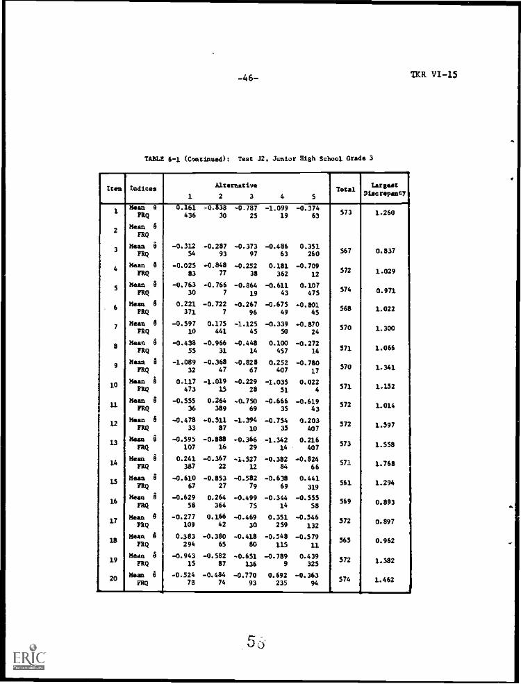
TABLE 6-1 (Coaticuted): Teat 32, Junior Ugh School Grade 3
TKR VI -15
Item /adices
1
Alteraktive
2 3 4 5Total
LargestDlacrepaacy
1
2
3
4
S
6
7
8
9
10
11
12
13
14
IS
16
17
18
19
20
Mean e
PRQ
Mean 6FRQ
Haan i
PRQ
Masa 8
FRQ
Mean 6FRQ
Meat 6FRQ
Maria 8
PRQ
Mean 6PRQ
Maw' I
FRQ
Mean i
FMHaan i
PRQ
Mesa i
FRQ
Mean 6
FRQ
Mean i
FRQ
Mean i
FRQ
Naas i
FMMean 6
PRQ
Hest 6PRQ
Maaa 6FRQ
Haan i
FRQ
-..-
0.161436
-0.31254
-0.025P 83
-0.76330
0.221371
-0.59710
4).43855
-1.08932
0.117473
-0.55536
-.0.478
33
.595107
0.241387
-0.61067
-0.62958
-0.277109
0.383294
-0.94315
-0.52478
-0.83830
-0.28793
-0.84877
-0.7667
-0.7227
0.175441
-0.96631
-0.36847
-1.01915
0.264389
-0.31187
-0.88816
-0.36722
-0.85327
0.264364
0.16642
-0.38065
-0.58287
- 0.484
74
-0.78725
-0.37397
-0.25238
-0.86419
-0.26796
-.1.12S
45
4.44814
-0.82867
-0.22928
-0.75069
-1.39410
-0.36629
-1.52712
-0.58279
-0.49975
4.46930
-0.41880
-0.651136
-0.77093
-1.09919
-0.48663
0.181362
-0.61143
-0.67549
-0.33950
0.100457
0.252407
-1.03531
-0.66635
-0.75433
-1.34214
-0.38284
-0.63869
-0.34414
0.351259
-0.548
115
-0.7899
0.692235
-0.37463
0.351260
-0.70912
0.107475
-0.80145
-0.87024
-0.27214
-0.78017
0.0224
-0.61943
0.2 03
407
0.216407
-0.82466
0.441319
-0.55558
-0.346132
-0.57911
0.439325
-0.36394
573
567
572
574
568
570
371
370
571
572
372
573
571
561
569
372
363
372
574
1.260
0.837
1.029
0.971
1.022
1.300
1.066
1.341
1.132
1.014
1.397
1.558
1.768
1.294
0.893
0.897
0.962
1.382
1.462
o

-48- TKR VII -1
VII Use of Index k* When Distractors Are in Full Work
It is obvious in Table 6-1 of the preceding chapter that for
these vocabulary items the knowledge or random guessing principle does
not work behind the examinee's behavior, for the mean values of 0
for the wrong answers are substantially different from one another
for most of the items. In cases like this, index k* , which was
introduced in Chapter 5 as a modification of Sato's number of
hypothetical, equivalent alternatives and used as an index for
invalidating three-parameter models, can be used as a measure of
desirability of the item for the group of examinees in question,
just as Sato's index is meant to be used for. An additional merit
of index k* when it is used for this purpose will be that it can
be used directly, without depending upon the relationship with the
probability for the correct answer, pR , which is illustrated
by Figure 2-1.
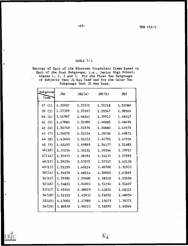
Table 7-1 presents the estimated entropy fife obtained
by (5.6), for each of the nineteen items and each of the four
groups of examinees, JH1, JH2(a), JH2(b) and JH3. The values
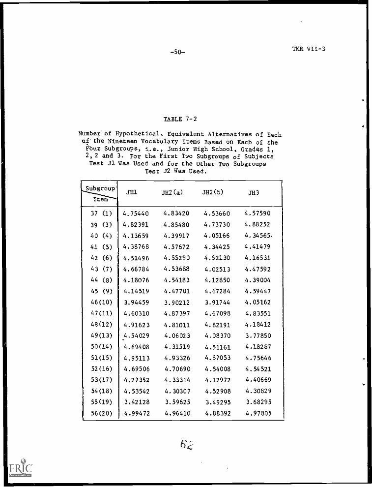
of index i* , which correspond to these fitos in Table 7-1,
were obtained by (5.10) and are shown in Table 7-2.
We can see in these tables that thirteen out of the total
of nineteen items have higher values of , and hence of i* ,
for JH2(a) than for JR2(b). Since the subjects in these two
groups are of the same school year, i.e., the second year of junior
high school, this tendency may be related with the fact that for SH2(a)
these nineteen items were given at the end of the test and for
6 ti
-49--
TABLE 7-1
Entropy of Each of the Nineteen Vocabulary Items Based onEach of the Four Subgroups, i.e., Junior High School,Grades 1, 2, 2 and 3. For the First Two Subgroupsof Subjects Test J1 Was Used and for the Other Two
Subgroups Test J2 Was Used.
SubgroupJR1 JE2(a) 1E2(3)
37 (1) 1.55907 1.57572 1.51218 1.52080
39 (3) 1.57359 1.57997 1.55547 1.58566
40 (4) 1.41987 1.48141 1.39913 1.46917
41 (5) 1.47880 1.52098 1.46885 1.48496
42 (6) 1.50740 1.51576 1.50880 1.42679
43 (7) 1.54070 1.51224 1.39256 1.49871
44 (8) 1.43049 1.51333 1.41791 1.47934
45 (9) 1.42195 1.49895 1.54177 1.52485
46(10) 1.37234 1.36152 1.36544 1.39912
47(11) 1.52673 1.58391 1.54137 1.57599
48(12) 1.59254 1.57072 1.57317 1.43130
49(13) 1.51299 1.40124 1.40700 1.32933
50(14) 1.54630 1.46214 1.50665 1.43095
51(15) 1.59962 1.59600 1.58320 1.55950
52(16) 1.54651 1.54903 1.51294 1.51407
53(17) 1.45244 1.46629 1.41821 1.48312
54(18) 1.51192 1.45933 1.51052 1.46054
55(19) 1.23002 1.27989 1.25075 1.30371
56(20) 1.60838 1.60223 1.58595 1.60504
6 1.
TKR VII-2
-50-
TABLE 7-2
Number of Hypothetical, Equivalent Alternatives of Eachof'the Nineteen Vocabulary Items Based on Each of theFbur Subgroups, i.e., Junior High School, Grades 1,2,2 and 3. For the First Two Subgroups of SubjectsTest J1 Was Used and for the Other Two Subgroups
Test J2 Was Used.
Subgroup
ItemJH1 JH2(a) J112(b) J113
37 (1) 4.75440 4.83420 4.53660 4.57590
39 (3) 4.82391 4.85480 4.73730 4.88252
40 (4) 4.13659 4.39917 4.05166 4.34565
41 (5) 4.38768 4.57672 4.34425 4.41479
42 (6) 4.51496 4.55290 4.52130 4.16531
43 (7) 4.66784 4.53688 4.02513 4.47592
44 (8) 4.18076 4.54183 4.12850 4.39004
45 (9) 4.14519 4.47701 4.67284 4.59447
46(10) 3.94459 3.90212 3.91744 4.05162
47(11) 4.60310 4.87397 4.67098 4.83551
48(12) 4.91623 4.81011 4.82191 4.18412
49(13) 4.54029 4.06023 4.08370 3.77850
50(14) 4.69408 4.31519 4.51161 4.18267
51(15) 4.95113 4.93326 4.87053 4.75646
52(16) 4.69506 4.70690 4.54008 4.54521
53(17) 4.27352 4.33314 4.12972 4.40669
54(18) 4.53542 4.30307 4.52908 4.30829
55(19) 3.42128 3.59625 3.49295 3.68295
56(20) 1 4.99472 4.96410 4.88392 4.97805
TKR VII -3
-51- TKR VII -4
J112(b) they were given at the beginning of the test. We can also
observe that, for some items, there exists a mild tendency that
the value of k* becomes greater as the school year increases, and,
for some others, this tendency is reversed. Items 39(3), 40(4),
44(s), 45(9), 47(11), 53(17) and 55(19) belong to the first category,
and items 37(1), 48(12), 49(13), 50(14), 51(15), 52(16) and 54(18)
are members of the second category. In spite of these mild
tendencies, however, the values of index k* are large, ranging,
approximately, from 3.42 to 4.99 , for all the examinee groups,
the result which indicates a high desirability of this subset of
test items for these groups of examinees.
We can observe a tendency that, regardless of the groups of
examinees, some items have higher values of than others, and
some other items have lower values of k* than others. Items
56(20), 51(15) and 39(3) exemplify the first category, and items
'55(19) and 46(10) are members of the second category.
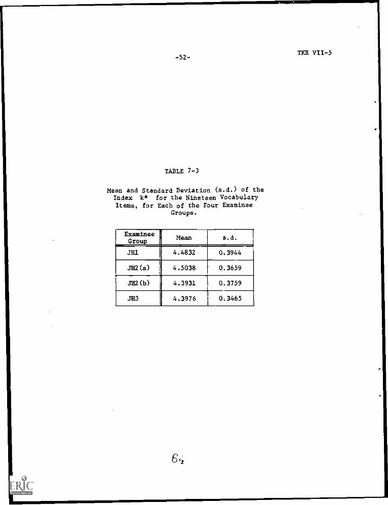
The mean and the standard deviation of the nineteen values
of k* for each of the four examinee groups were computed, and are
presented in Table 7-3. We can see that all the mean values are
between 4.39 and 4.51, and all the standard deviations are between
0.34 and 0.40, i.e., very close to one another, respectively.
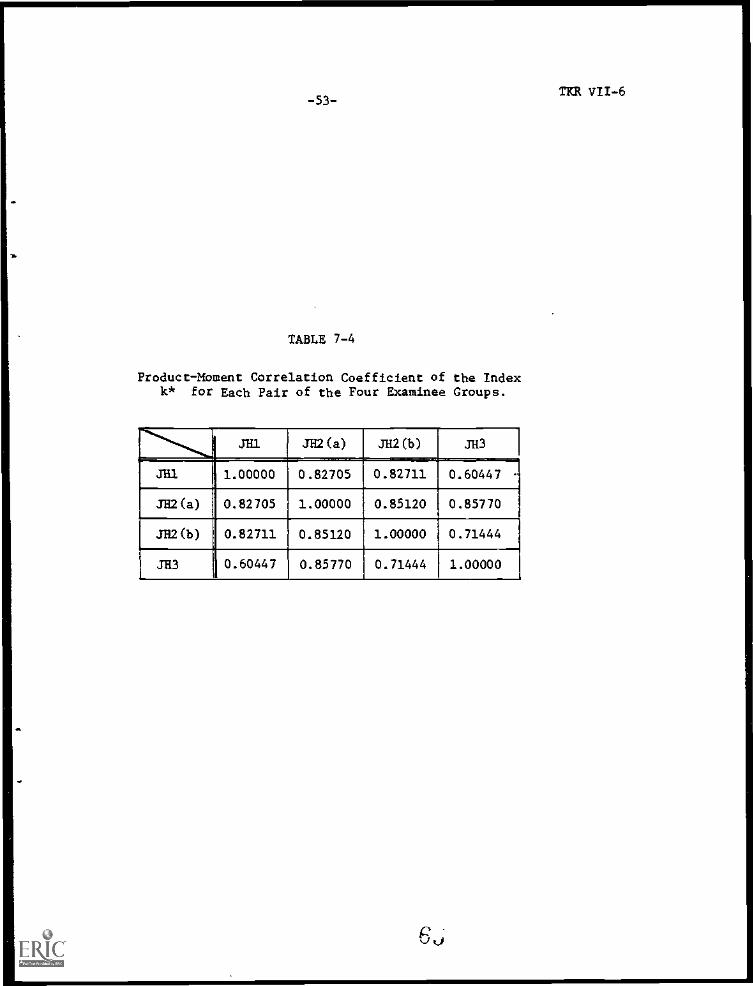
As an additional information, the product-moment correlation
coefficient of IZ *'s , which are shown in Table 7-2, was computed
for each pair of examinee groups, and the result is presented in
Table 7-4. We can see that these values are fairly large and
positive, as we can expect from Table 7-2.
-52-
TABLE 7-3
Mean and Standard Deviation (s.d.) of theIndex k* for the Nineteen VocabularyItems, for Each of the Four Examinee
Groups.
ExamineeGroup
Mean s.d.
al 4.4832 0.3944
JH2(a) 4.5038 0.3659
JE12(b) 4.3931 0.3759
JH3 4.3976 0.3465
TER VII -5
-53-
TABLE 7-4
Product-Moment Correlation Coefficient of the Indexk* for Each Pair of the Four Examinee Groups.
Al JH2 (a) A2 (b) JR3
Al 1.00000 0.82705 0.82711 0.60447
A2(a) 0.82705 1.00000 0.85120 0.85770
3H2(b) 0.82711 0.85120 1.00000 0.71444
JH3 0.60447 0.85770 0.71444 1.00000
60
TICR VII -6
-54- TKR V11-7
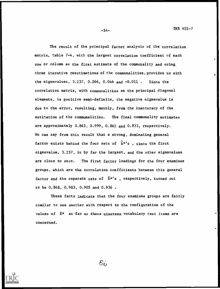
The result of the principal factor analysis of the correlation
matrix, Table 7-4, with the largest correlation coefficient of each
row or column as the first estimate of the communality and using
three iterative reestimations of the communalities,provides us with
the eigenvalues, 3.237, 0.266, 0.044 and -0.011 . Since the
correlation matrix, with communalities as the principal diagonal
elements, is positive semi-definite, the negative eigenvalue is
due to the error, resulting, mainly, from the inaccuracy of the
estimation of the communalities. The final communality estimates
are approximately 0.863, 0.999, 0.862 and 0.833, respectively.
We can say from this result that a strong, dominating general
factor exists behind the four sets of lot's , since the first
eigenvalue, 3.237, is by far the largest, and the other eigenvalues
are close to zero. The first factor loadings for the four examinee
groups, which are the correlation coefficients between this general
factor and the separate sets of t *'s , respectively, turned out
to be 0.868, 0.983, 0.905 and 0.836 .
These facts indicate that the four examinee groups are fairly
similar to oae another with respect to the configuration of the
values of 2* asfar as these nineteen vocabulary test items are
concerned.
PO
-55-TKR VIII -1
VIII Proposal of a New Family of Models for the Multiple-ChoiceItem
Throughout the history of mental measurement, the multiple-
cnoice item has been treated as a "poor image of the free-response
item," and very little accomplishment has been made in pursuing
its theoretical advantage, rather than its handicap. Most
researchers in these days mechanically adopt the three-parameter
logistic model for their research which is based on the multiple-
choice item, without even trying to validate the model. As long as
they continue doing this, we shall never be able to expect any
progress in this area of science, in spite of the fact that more
and more research materials and published papers are accumulated
year by year.
It has been one of the author's purposes of pursuing the
method of estimating the operating characteristics without assuming
any mathematical model a priori (Samejima, 1977b, 1977c, 1978a,
1978b, 1978c, 1978d, 1978e, 1978f) to approach the operating
characteristics of distractors, which are completely neglected
by the users of three-parameter models. While this approach is
undoubtedly more scientific than any othe7s, it will be desirable
to consider new types of models, which reflect psychological
reality behind the examinee's behavior in the multiple-choice
situation far better than three-parameter models and the knowledge
or random guessing principle.
The research on the vocabulary measurement made by Shiba
and others should be credited for the fact that they did not

-56-TKR VIII-2
accept the fashionable three-parameter logistic model blindly as
many other researchers do, and, moreover, they try to make full
use of the information given by the distractors to the extent that
they used it for branching examinees in tailored testing. As far
as we treat the multiple-choice item as a binary item, it will be
a poor substitute for the free-response item, which is contaminated
by noise or guessing. If we make use of the information given
by the distractors, however, the multiple-choice item can be more
informative than the free-response item, and will no longer be a
poor image of the free-response item.
The family of models that will be proposed in this chapter
is related with the graded response model (Samejima, 1969, 1972),
in which an item is scored into more than two response categories.
Let xg be the graded item score, which assumes Integers, 0
through m , and Px
(8) be its operating characteristic. The
graded response level can be classified into the homogeneous and
the heterogeneous cases (Samejima, 1972), and we can name the
normal ogive model (Samejima, 1972, 1973) and the logistic model
(Samejima, 1972) as models in the homogeneous case, and Bock's
multi- nomial response model (Bock, 1972, Samejima, 1972) as an
example in the heterogeneous case. In these models, the operating
characteristic of the item response category is defined, respectively,
as follows.
a (e-bx
)
(8.1) Px
(e) = (27)-1/2 g
g e- 'u/2 dug ag
(e-bx +1)
60
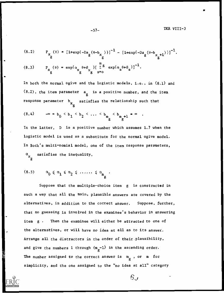
-57- TKR VIII -3
(8.2) Px (6) = [1+exp(-Dag(e-b
x))]-1 [1+exp(-Da
g(e-b
x +18
)}]-1.
(8.3) Px
(6) = expfa 8+8 1[ Zg exp(as6+8
s)] -1.
gxg xg
s=o
In both the normal ogive and the logistic models, i.e., in (8.1) and
(8.2), the item parameter ag is a positive number, and the item
response parameter bx satisfies the relationship such that
g
(8.4) = b0
< b1
< b2
< < bm < bm+1
oi co
g g
In the latter, D is a positive number which assumes 1.7 when the
logistic model is used as a substitute for the normal ogive model.
In Bock's multi-nomial model, one of the item response parameters,
xsatisfies the inequality,
g
(8.5) a a < a0 1 2 am
g
Suppose that the multiple-choice item g is constructed in
such a way that all the main, plausible answers are covered by the
alternatives, in addition to the correct answer. Suppose, further,
that no guessing is involved in the examinee's behavior in answering
item g . Then the examinee will either be attracted to one of
the alternatives, or will have no idea at all as to its answer.
Arrange all the distractors in the order of their.plausibility,
and give the numbers 1 through (m -1) in the ascending order.
The number assigned to the correct answer is or, or m for
simplicity, and the one assigned to the "no idea at all" category
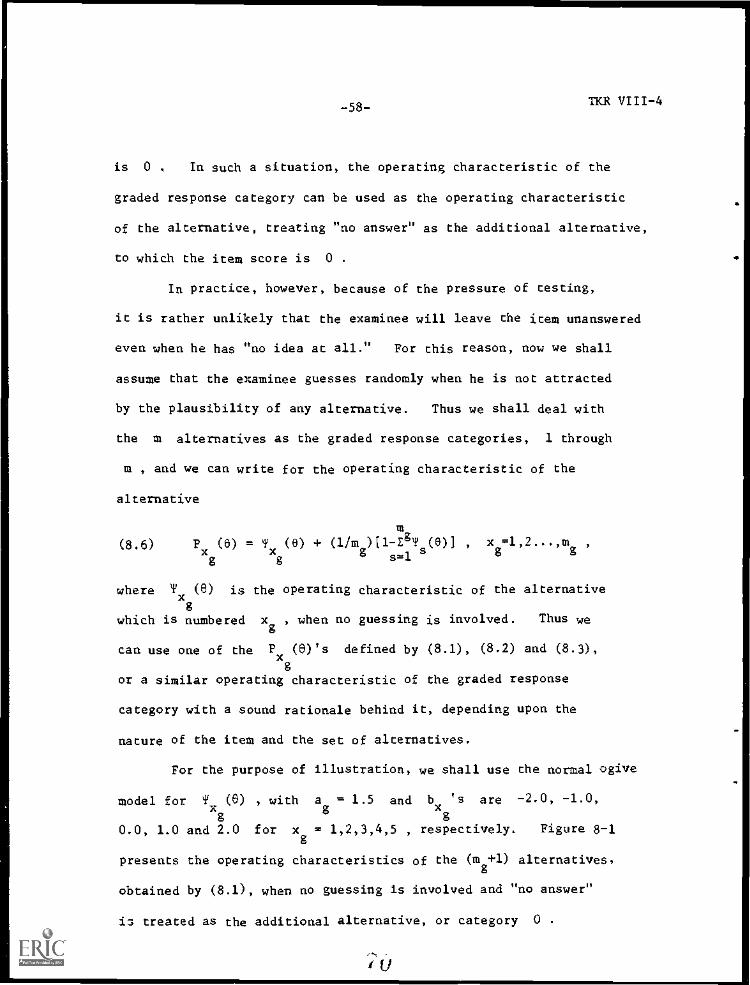
-58-TKR VIII -4
is 0 , In such a situation, the operating characteristic of the
graded response category can be used as the operating characteristic
of the alternative, treating "no answer" as the additional alternative,
to which the item score is 0 .
In practice, however, because of the pressure of testing,
it is rather unlikely that the examinee will leave the item unanswered
even when he has "no idea at all." For this reason, now we shall
assume that the examinee guesses randomly when he is not attracted
by the plausibility of any alternative. Thus we shall deal with
the m alternatives as the graded response categories, 1 through
m , and we can write for the operating characteristic of the
alternative
m
(8.6) P (6) = T (6) + (1/m )[1-EgTs(6)] , x =1,2...,m ,
g g s=1x x g g s
where Tx (8) is the operating characteristic of the alternative
gwhich is numbered x
g, when no guessing is involved. Thus we
can use one of the Fx(0's defined by (8.1), (8.2) and (8.3),
gor a similar operating characteristic of the graded response
category with a sound rationale behind it, depending upon the
nature of the item and the set of alternatives.
For the purpose of illustration, we shall use the normal ogive
model for Tx
(6) , with a = 1.5 and bx
's are -2.0, -1.0,
gg
g0.0, 1.0 and 2.0 for x
&= 1,2,3,4,5 , respectively. Figure 8-1
presents the operating characteristics of the Cm&+1) alternatives,
obtained by (8.1), when no guessing is involved and "no answer"
13 treated as the additional alternative, or category 0 .
l I/
.
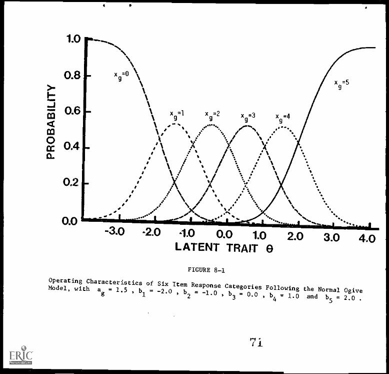
1.0
0.8>-1ca---.5
0.6ctco
cc 0.4a.
0.2
0.0
=X 0
\\\
a
1 x9
Xg
=2=1 x9
=3 x9
=4\ ,1,1 ' I ' \ a
% a.t e %%A
V
J._ ,4-i.1
i \i
4 1.
iis \
i 1 t i.% / .
. ..,% a %I
II 4?a. v
f A : % vf ItI %
..?f
00%
/ i t aa \
%%
oft.. ..._ 1...... ........
xg
=5
-3.0 -2.0 -1.0 0.0 1.0 2.0 3.0 4.0LATENT TRAIT G
FIGURE 8-1
Operating Characteristics of Six Item Response Categories Following the Normal OgiveModel, with ag= 1.5 , b
1= -2.0 , b
2= -1.0 , b
3= 0.0 , b
4= 1.0 and b
5= 2.0 .
71
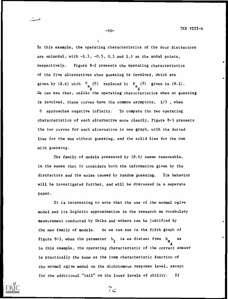
-60-TKR VIII -6
In this example, the operating characteristics of the four distractors
are unimodal, with -1.5, -0.5, 0.5 and 1.5 as the modal points,
respectively. Figure 8-2 presents the operating characteristics
of the five alternatives when guessing is involved, which are
given by (8.6) with Tx (e) replaced by Px (e) given in (8.1).
g gWe can see that, unlike the operating characteristics when no guessing
is involved, these curves have the common asymptote, 1/5 , when
e approaches negative infinity. To compare the two operating
characteristics of each alternative more clearly, Figure 8-3 presents
the two curves for each alternative in one graph, with the dotted
line for the one without guessing, and the solid line for the one
with guessing.
The family of models presented by (8.6) seems reasonable,
in the sense that it considers both the information given by the
distractors and the noise caused by random guessing. Its behavior
will be investigated further, and will be discussed in a separate
paper.
It is interesting to note that the use of the normal ogive
model and its logistic approximation in the research on vocabulary
measurement conducted by Shiba and others can be justified by
the new family of models. As we can see in the fifth graph of
Figure 8-3, when the parameter b1 is as distant from bm as
gin this example, the operating characteristic of the correct answer
is practically the same as the item characteristic function of
the normal ogive model on the dichotomous response level, except
for the additional "tail" on the lower levels of ability. If
.*".,
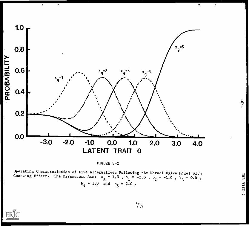
1.0
0.2
0.0
I .- . 9x9=3
9x =2 x =4
x 01 a* 0.--., _0.9 ,- % e '., de % e .
.. / t 'A
.. x1 % li: %/ ; % .. %.
N.% . \. .I. %. : . i
. / 6e.... ... ........
0. : \ . '46. %. .:. :
..- % \\..
.4.6..
x =59
..b % oo
-3.0 -2.0 -1.0 0.0 1.0 2.0 3.0 4.0LATENT TRAIT 0
FIGURE 8-2
Operating Characteristics of Five Alternatives Following the Normal Ogive Model withGuessing Effect. The Parameters Are: a
8= 1.5 , b
1= -2.0 , b2 = -1.0 , b3 = 0.0 ,
b4= 1.0 and b
s= 2.0 .

to
0.2
0.0-3.0 -2.0 -1.0 0.0 1.0 2.0 3.0 4.0
LATENT TRAIT 0
FIGURE 8-3
Comparison of the Two Operating Characteristics in the Normal Ogive Model.
x - 1.g
,i *1
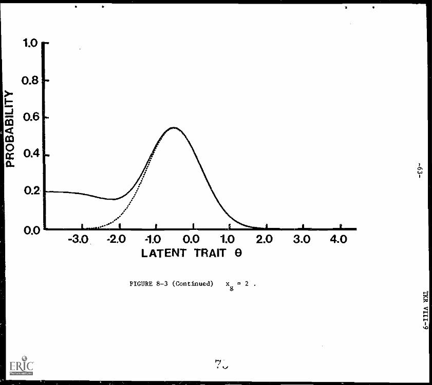
-3.0 -2.0 -1.0 0.0 1.0 2.0 3.0 4.0LATENT TRAIT 0
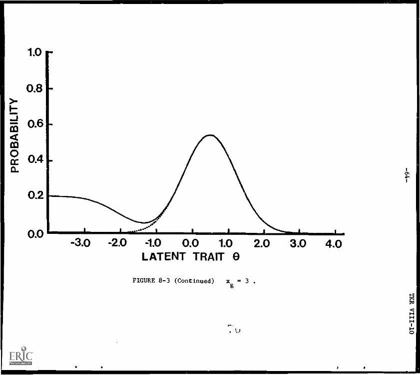
1.0
0.8-i:1m 0.6gtta0: 0.4a.
0.2
0.0-3.0 -2.0 -1.0 0.0 1.0 2.0 3.0 4.0
LATENT TRAIT 0
FIGURE 8-3 (Continued) x = 3 .g
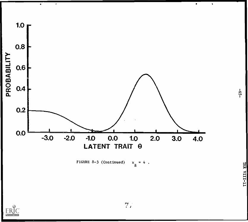
-3.0 -2.0 -1.0 0.0 1.0 2.0 3.0 4.0LATENT TRAIT 0
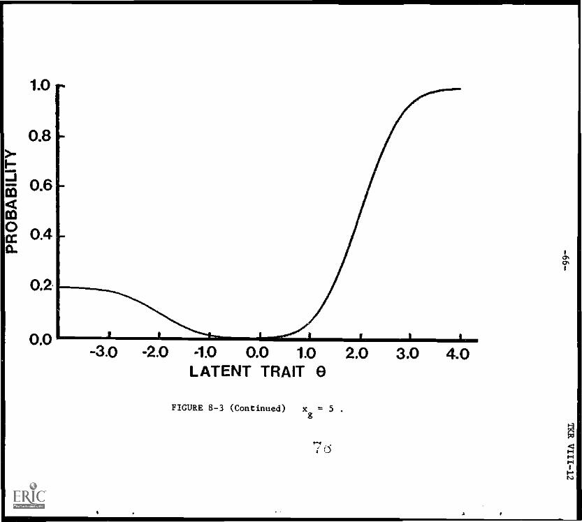
-3.0 -2.0 -1.0 0.0 1.0 2.0 3.0 4.0LATENT TRAIT 0
-67- TKR VIII -13
this is the case with all the items in the test and the ability
distribution of our examinees does not include lower levels of
6 where these tails lie, we can approximate the operating
characteristic of the correct answer by the normal ogive model
on the dichotomous response level, and use the tetrachoric correlation
coefficient and the logistic approximation and so on, just as Shiba
and others did.

-68-T1CR IX-1
IX Discussion and Conclusions
We have introduced Sato's number of hypothetical, equivalent
alternatives, and defined its modification, index k* , as a measure
of invalidating the three-parameter logistic, or normal ogive, model.
We have also introduced Shiba's research on the measurement of
vocabulary and the construction of a tailored test, using the
information given by distractors. Various observations and
discussion have been made concerning the three-parameter models
and item distractors, the validation of mathematical models, and
so forth. Finally, a new family of models for the multiple-
choice item, which formulate both the operating characteristics of
distractors and the effect of random guessing, has been proposed.
There is a tendency that researchers restrict their ideas
within the tradition of their own culture. Thus they tend to
accept whatever is familiar to them, what is fashionable among
other researchers in their culture, and so on, without feeling the
necessity of validating the ideas and mathematical models in
relation with their specific data and psychological reality.
The virtue of doubt can be obtained if they shift their attention
to what is going on outside of their own culture and climate,
and try to think what is really right.
Three-parameter models for the multiple-choice item have
been too readily accepted among psychometricians and applied
psychologists, and they have been using the models without trying
to validate them. Unless we correct this wrong orientation,
psychology will never make any progress, regardless of the fact
80
1-69-
TKR IX-2
that more data are accumulated and more papers are published year
by year. In the author's opinion, psychology has not yet established
itself as a science, and we need to do that by putting ourselves in
a right track of research. In so doing, the validation of
mathematical models is certainly one of the most important things.
The departure from the tradition should also be made in the
treatment of the multiple-choice item. Instead of trying to handle
the multiple-choice item as a "blurred" substitute for the free-
response item, we must make full use of its advantage, which the
free-response item does not have. The operating characteristics
of the distractors of the multiple-choice item will add more
information about the examinee's ability level. We must set
a criterion for the quality of multiple-choice items from this
aspect also.
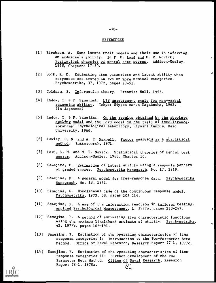
-70-
REFERENCES
[1] Birnbaum, A. Some latent trait models and their use in inferringan examinee's ability. In F. M. Lord and M. R. Novick;Statistical theories of mental test scores. Addison-Wesley,1968, Chapters 17-20.
(2] Bock, R. D. Estimating item parameters and latent ability when 4
responses are scored in two or more nominal categories.Psychometrika, 37, 1972, pages 29-51.
(3] Goldman, S. Information theory. Prentice Hall, 1953.
(4] Indow, T. & F. Samejima. LIS measurement scale for non-verbal_reasoning ability. Tokyo: Nippon Bunke Kagakusha, 1962.(in Japanese)
(5] Indow, T. & F.. Samejima. On the results obtained la the absolutescaling model and the Lord model in the field of intelligence.Yokohama: Psychological Laboratory, Hiyoshi Campus, KeioUniversity, 1966.
(6] Lawley, D. N. and A. E. Maxwell. Factor analysis as a statisticalmethod. Butterworth, 1971.
[7] Lord, F. M. and M. R. Novick. Statistical theories of mental testscores. Addison-Wesley, 1968, Chapter 16.
(8] Samejima, F. Estimation of latent ability using a response patternof graded scores. Psychometrika Monograph, No. 17, 1969.
(9] Samejima, F. A general model for freeresponse data. PsychometrikaMonograph, No. 18, 1972.
(101 Samejima, F. Homogeneous case of the continuous response model.Psychometrika, 1973, 38, pages 203-219.
[11] Samejima, F. A use of the information function in tailored testing.Applied Psychological Measurement, 1, 1977e, pages 233-247.
[12] Samejima, F. A method of estimating item characteristic functionsusing the maximum likelihood estimate of ability. Psychometrika,42, 1977b, pages 163-191.
[13] Samejima, P. Estimation of the operating characteristics of itemresponse categories I: Introduction to the Two-Parameter BetaMethod. Office of Naval Research, Research Report 77-1, 1977c.
[141 Samejima, F. Estimation of the operating characteristics of itemresponse categories II: Further development of the Two-Parameter Beta Method. Office of Naval Research, ResearchReport 78-1, 1978a. X),
-71-
REFERENCES (continued)
(151 Samejima, F. Estimation of the operating characteristics of itemresponse categories III: The Normal Approach Method and thePearson System Method. Office of Naval Research, ResearchReport 78-2, 1978b.
[16] Samejima, F. Estimation of the operating characteristics of itemresponse categories IV: Comparison of the different methods.Office of Naval Research, Research Report 78-3, 1978c.
(17] Samejima, F. Estimation of the operating characteristics of itemtesponse categories V: Weighted Sum Procedure in theConditional P.D.F. Approach. Office of Naval Research,Research Report 78-4, 1978d.
(181 Samejima, F. Estimation of the operating characteristics of itemresponse categories VI: Proportioned Sum Procedure in theConditional P.D.F. Appr-ach. Office of Naval. Research,Research Report 78-5, 8e.
(19] Samejima, F. Estimation of the operating characteristics of itemresponse categories VII: Bivariate P.D.F. Approach withNormal Approach Method. Office of Naval Research, ResearchReport 78-6, 1978f.
[20] Sato, T. Engineering techniques for analyzing educational data,No. 5. Central Research Institute, Nippon Electric Company,Ltd., 1977. (in Japanese)
[21] Shiba, S. Construction of a scale for acquistion of word meanings.Bulletin of Faculty of Education, University of Tokyo, 17,1978. (in Japanese)
(221 Shiba, S., Y. Noguchi and T. Haebara. A stratified adaptive testof verbal ability. Japanese Journal of Educational Psychology,16, 1978, pages 229-238. (in Japanese)
[23) Tatsuoka, M. M. Recent psychometric developments in Japan:engineers tackle educational measurement problems.ONR Tokyo Scientific Bulletin, 4 (1), 1979, pages 1-7.

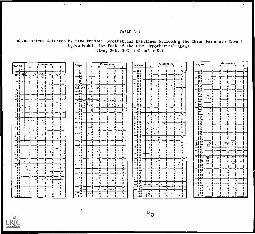
Co
CIL
1 I ..-
.4 +
.4-4
,4.#
pw.W
ww
m6.
6.1.
.u..L
ftpof
t.4.0
.N.
.4. .
....
II. ,
II
'
......
-04.
,,..
II
Iv.:'
'.1 ......
'.
10.0w
11
-...
I/ WN.0
1
--
- ,
ri .-...
.-..1
.0.
0.0../.0
i%
I,
.....
/i
I..,
ft
I Pw0W..
I/
Vt.
I> I.P.
A
i r
1_ r
,.....
..14.
..I
,A.R
1..
..,r....r...4.....r1...J.
4'11
:I
1
,.....
IQ.
.t..w
.
II
+4.
10p1
7
'.. 7 ..
, #.-.
4,ow
.," ......
......
....
I i .L....
1 I1 -?-r
w.
.,
"'" a.
,:
II
I eaft
w.O
...,6
1...,
or00.WWW..
'-'
,.,,
, .
.....1
...
1 I :
.
. ....
..
.
......
4 L
1 L
1,
II..
.. .....
. LW0
II
It ? illx.:;-.
1;
p L....._
II.J
I..p..
L
_.I
ir
1
1 .....
II
1 1I
i'
41..
- St
..._
..,
b.4
17.
..L.
a
et erI
sji.LI.L.1...1...51.1.1.1.
0 .......r.000_,001!frw.000
.I
-._
Ii
;.1.1
....
......
,11.
.0.,.
..i...
.1.4
.41.
,.6.4
0....0. ........
I
.....rowe....
I
IL
i isi
,:
.
w.
S
.......
. A
...h.
..
N ..
%pi
..L
J.
[ii.
r 1
12.1
.1I.
...ro
d...
....
...
.....1
I.
li
L4.0.00.
:
IL' ' ..'
,,. 7....
....."
w,
Ii ...6,
...r
II
W!..1.0.06.
1
L I y fl!,
ri!
'.1
....f.:
,'
...
IL i
Li II
.... 4.,..
.
.10
....I
,.-
. ...
L LI .,.
IW
hoe.
O..
1.1.....
-..,..,.....,;
s
,,
I, 1......,
IL
.... L
,
,... '
-...,
_.......
$.00
;
..
..,..
.....L [...,
1.0,
..
. ... t .494
1/1.
.; .o..*
tr'w
.lp..
. 1
,
.. ....e
.:. .... ..."
n ...
"1
r..t.r#.1=44t11....v.s.w....e
I.' iL
.'L
'-1..-
."L
I' L
.*--
LL
I
1
I
L."
L''P
D.!
".1.
:L'
lI
v.LI
Ip-
..
.4
..4.
.....
r'...
....
....
..-
......
.r
...
Li....
...-
I..
.-
1. w 1.11-.
LII..,...1,.....
L.
..
.V ......
..#4-
[ - -IIL 1 L
.4.1.1-....
1
,
I1
;
te:
.V
L--
- .
Li.0
..1 wit.
.;...
I
I'
LII ....
...
LLI
..
'
,,,L
, , ,
. . L
1't
1.0.
.,0
4....
:::
...
.[..,
tA
. .(.4
,#.p
..#L'..
i ,
r.
I,
[I
."N
. ..1
0.4.
wI I
.....:.
-.1...1....1-L.
1
...... ...,...
....
11
1 6.1
L:
...F. d, ...
p
1 . P.N
..I
IN
..11.1.....i
.
_
OW
LN
IA
tpo
41.:1441t
, Pi,
r 1
r ,......-.
I1
Li [
.- ..
, ,
1. .
.....
L.1,1".-1.'
,1 It ,r
iI
Li_
I-
ea
.. .. .
,Pi
! ... 10
4.
.. .........,....v.
i L - 1..?,,,
10
--;1.1.
.' , ....,
7,
NI ............
ft.I
.NN
.-- ..
.' I : I .
.....
W.N
#4.4
.W."
.
.i.
.
FYN.
....wit...
......
.4;::...-,,-
..r
to:..
I
.
. /
.- H MN
A
11.0.,
.
7 0, .. ..
a. a
.
a. ..
6. 1 .
. a. N
.
.. ,..
...J.I
..
a. a.
ft.
-, I L
. r J.
1.
, a . ._ 1%
;
41
rt I
ft II * Pg ft 4 CO t) lb lb ft lb 0.
0a 01* 4.
" CO
0 a. CD
O.
er
rto M
110
0.D
> 1
-t
hg P
a *C
111
n 0
to m
. ft
oIr,
ttr,
11er
j try
CO
X toto
CD
S fDtr
ot"
CD
II0
(ft
L-4
1rr =
-0
Fr I
.n
0 E
1-i c
oft lb B (0
P.
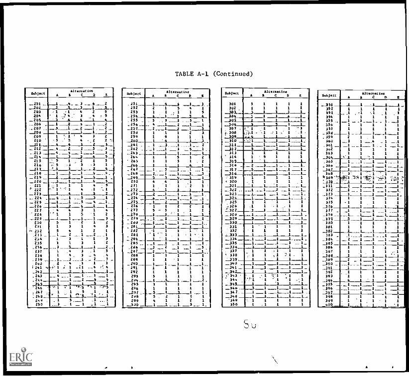
141
:....... 1**..41*PIMmom*,*
..
4
..........J.J...........L.14.1.i......1..;,.....
1
,
...
..
...1 ,
1
....
1
--
_: ij 1:11............I 1 1
;t11
1111
... ....
III..1.1.-
I
11; ; ,
ift._!I14.
141
I
1
.
i 11
0.1..
III'-,,,
...M.
... 11,
MH
..
Fl
!I
..!
11r
..
....
-- .
11 j.IIIin
11 ...
1
..
...
'1
lij1 u.
III1---
rrr
1
-
:. 1 . f
i![ j II 1 i .
VeletWa.T.:=:!=:it=ttitt42=Agg::::+:1r;74 .,.....1....w.m9^w...N.,0,^Am,.A.mm...49,q..,%.mmm,..mmm,...iii.. M.. If if'. if 1 i..1dlif ..ifi..iff..... I
177;:gif i r .
..4.
: .,
.4
-:-......1I
.41
;
1jr4.8
._Y
1
n -,4-:II
1 1
. .1...1%1 1
P
.....
MM]
'
.
. . j -1-NII41.4.4
lo
-,n ...
1!11
11
.411
...a ....
I III
ii..:
$
. 1
;.4,4.4
....,
f . '444.4.61,,II11
II
IIi
14111
,4
. t..
....IIi
1
......,
i
1
I
1
.... ...liN'j
.:- ill F
1
:1
1
.1.
1
i.4.. .. ...' I 1 I
1
111..: I
i
1I
I
'11. i,
VINWM
. !. I
-4p..Po
A
- ,
1
..I i ,
.44^ ..0 .00.0.4^0..mo.-ft...... epppephimpimpp.m..ft
'
J.PI 14;1
,
. IFf
11 ............. 111.4..1,4,fl}olg....2:4,4-
1 (
etZZA
: [ 1 iI
. 1
.. cii. imi*op..***1. ftetort'rorTiZTAZZAZAry1491i 1
.
*
W
Op
NO
41..41
...k
i....,..1.....
..
:
1
...
Ne.414,4NOMM
I I
11
4.1 .41 ii...
/11
4
I .wk...
.1M
I
El l
I 1
1111'
$
I i
ji11.11111.......
' ..;"
1
1 1 1
moi4147 ill1 1 HO Irt . l
II/ WI ......1 4 ''.
it1 .. 1 1 ! I .:±i
I
1 I
1'11i
/ j ..11q... ......1 ! ..
I 1 ', I .
, , . ..,
6
..I
1
.r
pwpipppg
_]
...
_..
.,
*4
O
I
....I**********Tr"
....... o ..ItW. . 0
4Ili I'lleel,* .. pi .. .O.. ..
: 1 F /'
O.N.J. 0...**...Ps*s1
'
Pio.o.P.Pin.1*
...***
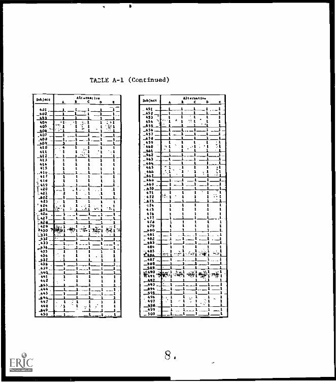
.eh
.4 7.7..1
]----11...,. .
.0 miI
! I
.4 .
.....d. v.v....44.i
1
,-
4..4. ....err
II
II ...f
... ..
...1...]..11....7
.. 44
1
. .. .....
I 1 1
III ,
ill
1 1.......441....
........I
I . 1 i
:.
-...-
...
.....
j,..1
i
1
A 4.4.0 4.1141.14.4.11.114 4 411114 ,..
r .40..
.3.1.
..,-.p.07.Nm4W0P.Ooe,
411.0ti lig.0 4% 4.14lit.-494 In
!I
4.,
IllIM
......, 1....H....1.1
... wj '''g
I
.....
1.1 I j
I....,
ii
...wt.. ......
.0
1
I
__T.:"
!
C......
.4.80 4..
-..1
. .......
1.., ...,
.o 71.....
0Pv
,...,
7
11....I ! j
i!
lej
I
I
.6..
_
........
. ....I
11
1111:.
Ir,
.0
.
V- .qoes .0s. 01" .0 70 0 04 ....._.,,14:114.4.1..t..,.....,:n..,....1......1
7 I1100.,nd. ...... J ..... .........1-111-414

-76-
APPENDIX II
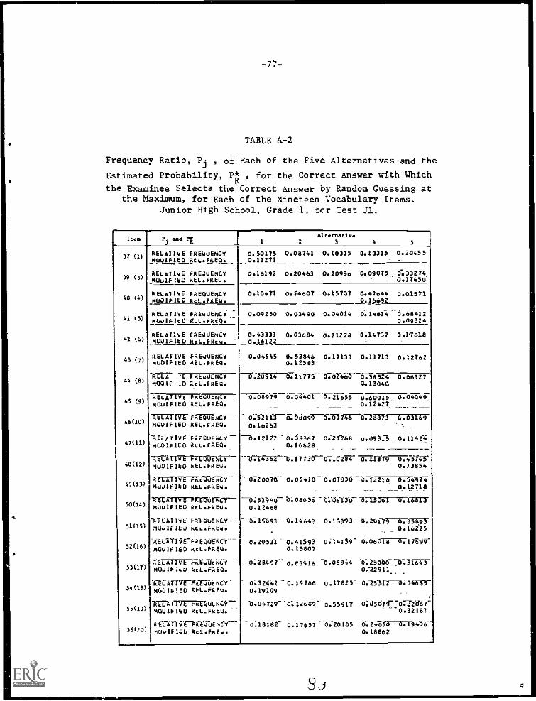
TABLE A-2
Frequency Ratio, 'Pi , of Each of the Five Alternatives and the
Estimated Probability, P* , for the Correct Answer with Which
the Examinee Selects the Correct Answer by Random Guessing atthe Maximum, for Each of the Nineteen Vocabulary Items.
Junior High School, Grade 1, for Test Jl.
Ices P and PaaAlternative
1 2 3 4 5
37 (2) RELATIVE FREQUENCY14901P IE 0 Ai k.F841.._
-0.50175 0.08741 0.10315 0.10315 0.20455
--
39 `"aEt.611vE iREJJENCYFWD/PIED kti.F8E0.
.0.1327/
0.16192 0.20463 0.209% 0.09075 ,,, 0.33274,0.17450
40 ", RELATIVE FREQUENCYmi.o211E0 8t1.F8Eu.
0.20472 0.14607 0.25707 0.47644 0.015710.16692
R ELAI 1 V E FREQUENCY 0.03490- 0.04014 0.14834 -0.6841241 (5) ni_otici3 g1.1..iiciQ 0.09324
, nEt.A71VE FREQUENCY 0.43333 0.03684 0.21228 0.14737 0.2'701862 (6) .4001F ZED ktLF1(cw 0.26122,43 `"
aeL Ai lye FREQUENCYPDDIF 1E0 Ai i.fice0.
0.04545 0.53846 0.17133 0.11713 0.122620.12583
12 41-.7 'E FREQUENCY 0.20914 0.21775 0.02460 0.58524 0.0632744 (8) 1001E :0 ;41.FRE0. 0.13040
45 (8)117./J10=(60,Wio4.)if le0 RELFiliecl
0.08979 0.04401 0.21655 060925 0.0404510.12427.
., 1161.A1 IVE -Frffi,TENCV 0.521 /3-0.06099 0.07746 0.28873 0.0316946("' n001F 1E0 kEi..20. 0.16263
67(11)SLAT IV E FtQ UE4..YsiD i a o am.. meg.
0.12227 0.39T67 0.211 sa 0039 31 5_ 0. Li ,.24 i0.16628
.
-1-ErATraATIFIENY -6:11S63 -6. 1 7 7 3V-07i Oar oi879 . 4 514368(12) 1D01P 1E0 Ati. F8E0. 0.13854
A-errET 1 V E Peki0-aftia --072007o 0.05416- 0; 0/333- b:TaT6-6:3-417T48(13f 04th.01i1E0 ati.akE:i. 0 12718._ . ..
k-EEKT-mFraTurary- -el; a-v)40-- 2): oa 0 so b O6-130 013061 -o-. rarr5004) Pi0uIFIED Rca..14tEu 0.12468
-VE Oil i V1--R-E0TA &VI- 6; U893- 0.14643 D.15393- V. 10 C71-b7311cf51(15) :40.02F It0 Kt i.F.t.. 0.16225.. _
52'4'kaaaaltir FA G:Mita-i40v11:160 KcL.F3e0
0.20531 0.41593 0:24159" 0..060W0717Vir0.15807
;,11:11TITE-1-Tamucm.y 0:26497- 0.06516 0.05944 O. 2506670-Z16-Cr33(17) 10.,IF hp kc L.Fkao. o:22917
IZECATIVE-Fgrai NO(' 0:324'42 0.19786 0.27825 o.-25-mr-G:a4z-s3-54(18) 140011E0 REl.Ffiiti 0.19109
,
55(19)iti AlT EiKEDUinii-401IF IED 8E..FnEd
0.06729 a; 126o9" 0.55517 0:6soIc0722017-0.32187
an-AMTE--PeTEZJENCY--- 0.18182` 0.12652 0;20/05 4: Zji50-171940656(20) mu.,1F1E0 Rti..F.a4. 0.18862
Sul
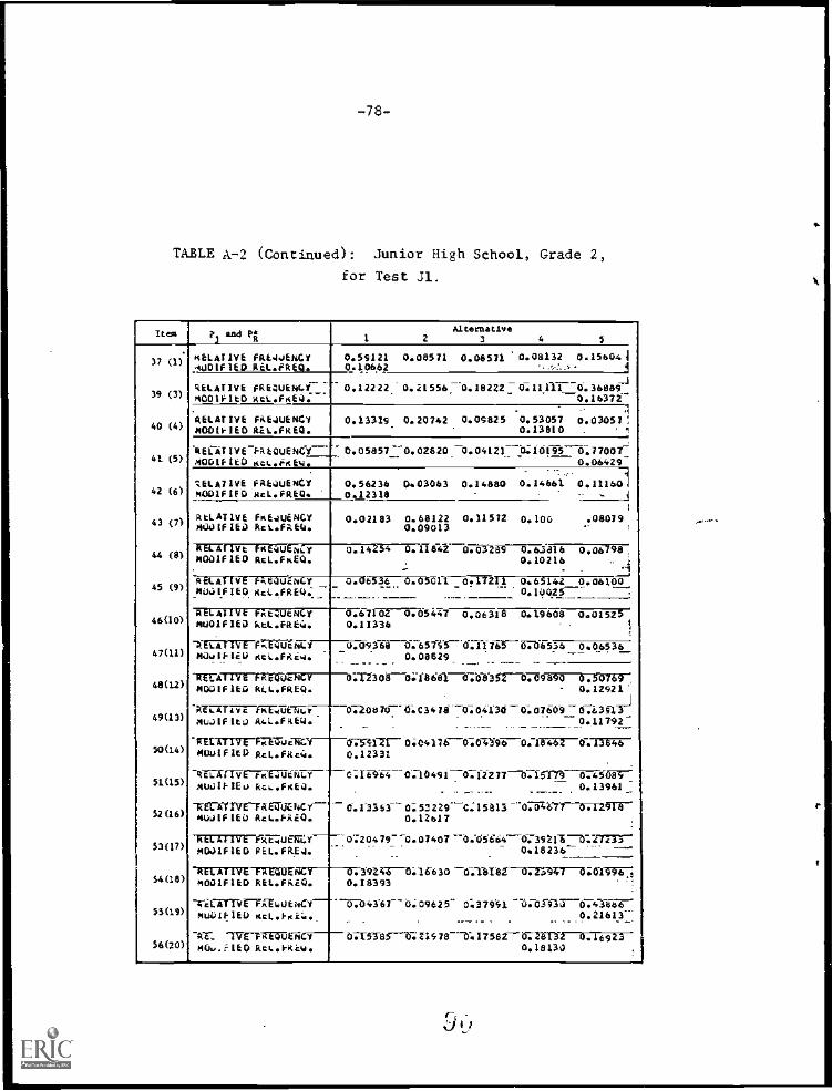
-78-
TABLE A-2 (Continued): Junior High School, Grade 2,
for Test J1.
It ? and PA1 R
Alternative1 2 3 4 5
7 m.3'
KELaTIVE FRA.IdENCY 0.59121 0.08571 0.08571 0.08132 0.15604 Js'" -10DIFIED ReL.FRE0. 0.10662 1-i
-0..36889.39 (JP(3) RELATIVE FREQUENGY:-
P4001F1E0 REL.FAED.-0.12222 0.2155670.10222: 0; 1111.1
0.14372-.!RELATIVE FRE.10E140 0.13319 0.20742 0.05825 0.53057 0.03057;
40 (4) MI3011-1E0 REL.FREO. 0.13810 . 9
RE1aTIVEFREQUENCY- b.058577_0.02820.-0.04121.__b;i6195-1;77007-41 (5) MOOIFIED KCLhtbi 0.06429-
42 (4'(6)Elal LYE FREQuENC.Y 0.56236 0.03063 0.14880 0.16661 0.111601MODIFIED Mel.FREQ. 0.12318 -i
I,41 %"
REL AT 1VE FaE.LANCY 0.02183 0.68122 0.11572 0.106 .08079MODIF lea ReL.FRED. 0.09013 .-
1
RELArivE FKEDIANCY 0.14254 0.11842 0.03289 0.63816 0.00 98,44 (0) MODIFIED REL.FaEQ. 0.10216- . .
RELATIVE F,E04JENcy 0.0651F7707B013 0:71714A 0.65142 p.0619049 (9) $1041F160 14eL.FREQ. 0.10025
46(10)REL Ai 1 Ile FAL:r.UENCY 0.6716ETIZO5447 006316 0.196081:L.015--.PitiO1F IED 1tl..Fa8 4. 0.11336
-altir, ITUFZEWEL11.9 0.0653647(11) MaulF120 AcL.FAew.
_0.06311-0.6sic5-0.1;11.3-F.-0.69.260.00029
lrEral Iva FRE(hotracy 0.17308 (1.18681.01-397-0769 890 0.3076948(11) MODIFIED ki.L.FREQ. - 0.12921'
a7:3715777-7a74vEN1;.. 07208 107 0: C3 4 1870; 04130 0. 0 7e09 07,6 3 STIlj49(13) MuDIF 1E0 AL.FREi.I.- 0.11792-
- - - .........- ....- ....--._.1110117E-FraTuaLY G-5-11zr- 0.04176-0-.07.)-976-0.0.-1317:6
50(14) mulFIED R.L.Fx.4. 0.12331.
R 1 1 7 K C I V E r r i r . I T E F i t i 0 ; 0 0;10 49 I -0:122 7 7-015-1-n---.37r.sa-c_51"'' MUD IF Hu REL.FnED. 0.13961
-rECOIVE-ramuchey-- -cia3363-0:53229 "-C:151313-01-2411-S2 {16) GuLAIF 1E0 Rel..F/i2Q 0.12617
33(1"661.Arive Att..UENZ.9-- 0;2 04 79-0. 0 7 407 -0 ..0 5644--ISZ39 2 1170:27rIc 75-MOJIFIEO REL.FRE.). 0.18236----661.61-tv6 I-R etruEnCr 0. 39141-0.1 6-6 30 -0alltr--o-zrpg-i-a . ai-§947;
54(18' MOOIFIED REL.FAeL). 0.18393
-rearlia-Fai.DENC11--- 074341- '0: 09625- 0;3290,. -13a,91 3 0.7.:314-6--5s(19) ML4(1 6c1.0-Ki;.. 0.21613-
56(20)la "IVE7 grZET- 015335-0: ZI 9 7 --. I 7 582 GUM 0.16923MO...i'IEO REL.I-Rew 0.18130
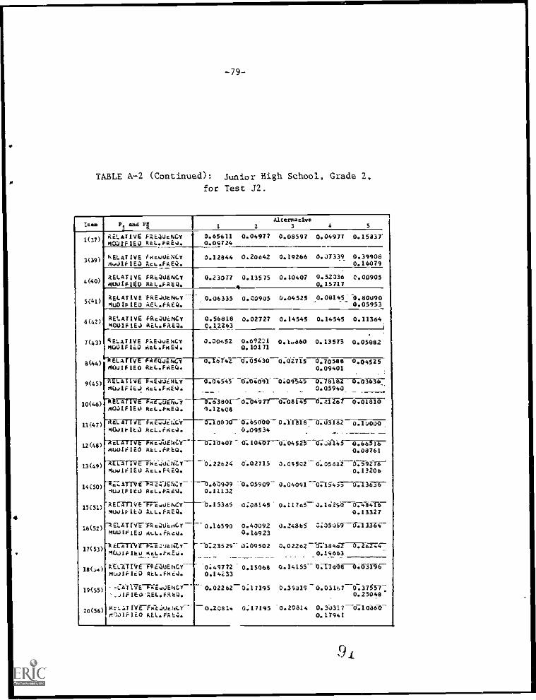
-79-
TABLE A-2 (Continued): Junior High School, Grade 2,for Test J2.
4(40)
5(41)
RELATIVE FR62061.476(42)/-
0,1001P 1EJ aEL.FAI5.
7(43)
B(44)
9(45)
10(46)
11(47)
12(48)
13(49)
14(50)
15(51)
16(52)
17(53)
18(x4)
14(55)
20(56)
P and Pi
RELATIVE FREQUENCYM00IFIE3 RELfRE.I.
kELATIVE l'itewieNCT3..4)IFIE3
RELATIVE FREQUENCY.100IFIE0 ReL.FR).
RELATIVE AE40tPielrMuDiF1E0 REL.FREQ.
RELATIVE F;sEQuENCTmoOlP LEO Rtl..FREQ.
RELArivE'Wulf TEO Rti..FRE(.
"ETA i vE TREtitIcriLvAiwa 4E41 Act...FREQ.
AltermAcive2 3 4 5
0.65611 0.04977 0.08597 0.04977 0.15837*0.09724
0.12844 0.20642 0.19266 0.J7339 0.399080.16079
0.23077 0.13575 0.10407 0.52036 '0.009050.15717
0.06335 0.00905 0.04525 0.04145 0.800900.05953
0.56818 0.02727 0.14545 0.14545 0.113640.12263
005652 0.6920.10171
0. k..abo 0.13573 0.05082
oA5430 Gouts 0.70588 0.045250.09401
0.04545 0.04091 0;09345 Cl1sTer-570363-67.0.05940 _
TLATIVE FAc..ugn.Y 1- 0.6340I-070497167011f4TWEra15.01810roO0LFIE0 RtL.FwEO. 1.12408
RE:71-c).CV 0.10030- 0.65000 0.11818. 0.03182 0.100000010160 ReL.FA6.). 0039534
clATIVE FAcRatiCV------0:1.43407 106-07-G0452-5 0..)8142.656/41b01f 1E0 ReL.(4.h0. 0.08761
AnIT-IVE-1ro6-4dai-C.7.--- -0:22624 0.02715 0.05502 0.05881--67592-76MuuleIEU ReL.V4EQ4 0.13206
eZ1179E-F3:714.1V-6..T -0.6'0909 .0.05909- 0.04091 -ons4,5-0.11c7r6--AuJIF lit) Rei..FaeQ. 0.11132
RECI714"E-Fre-dUEAC-7 I.L5385 0:08145 0.11765-.3.1 c 2$1:T 7.74,14.71-6-mualIFILO t.LL.FT.EQ. 0.13327
1.7.TP(E-Frie3t)E0CY-- 0.16590 0.40092 0.248135 5: 55 t) i9 1 Int:muu Ts: 1 Eu ALL.Fkcti. 0.16923
ft tarn E-FVE -0:23529 0:09502 o.o2zoz-o73sio7-6.707474-1:mcwiftku 0.19663
L'A-TrciunavErIcy---- 0.49772 0.15068 0.141550:77644-0.01-16-mLoif Lep ReL.Fke.}. 0.14233
zt:ATIVE-Fr;E.WENC-7-- 0.02262-0:17195 0.35319 0.031670.37557IEt7.1.EL.Fatg. 0.25048
H: L:11VFxeaUellLY" 0.20914 0:17195 0.20814 0.34317-W108670-Y.:JIF1E0 REL. Fa 0.17941
9
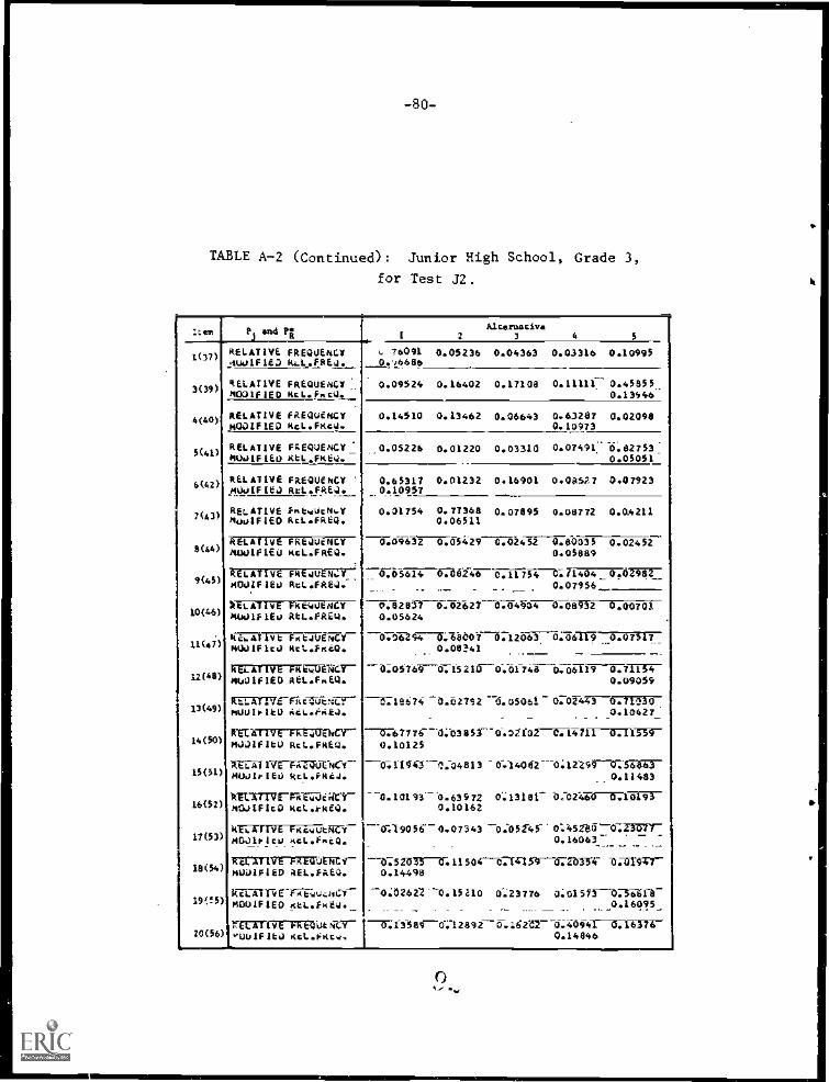
-80-
TABLE A-2 (Continued): Junior High School, Grade 3,
for Test J2.
r.t.n. Pj sad PoR
AIcensaciv.1 2 3 4 5
1(37)
3(39)
4(40)
5(41)
6(42)
)7('
8(44)
,,.,9""
10(46)
11(47)
12k--,
13(49)
14(50)
15( 1)
16t52,
11 '7) '
18(54)
....191
29"4'
RELATIVE FREQUENCY4UOIFILD lit.L.FREQ.
A. 74091 0.05236 0.04363 0.03316 0.109959j,v)4486
RELATIVE FREQUENCYNO3IFIE0 14cL.F.012
0.09524 0.16402 0.17108 0.11111- 0.458550.13646
RELATIVE FREQUENCYNQUIF LED 1cL.Fttc61.
0.14510 0.13462 0.06643 0.6)287 0.020980.10973
RELATIVE FREQUENCY000.11FIEU RE!. .FNEQ.
0.05226 0.01220 0.03310 0.07491 6.62753_0.05051
RELATIVE RFLEOUF9tEENGIY. 0.65317 0.01232 0.16901 0.08S27 0.07,230.10957
RELATIVE fmtmlicr0.4SuaIFIED RcL.FREQ.
0.01754 0.77368 0.07895 0.08772 0.0.42110.06511
RELATIVE FREQUENCY400IFIEU NcL.FREQ.
0.09632 0.05429 0.02452 0.00035 0.024520.05089
RELATIVE FREJU NE
HOUIFIEU RtL.FREQ.0.05614 0.08246 0.11754 C.71404_ 0,01742=
- - 0.07956.. ...... _ _MAUVE- niEwtricyNUOIFIEy Rti..FRita.
o,ezer-o.ozort 0.4)4904 o.osriz 0.007010.05624
It-E.Trlit.itlEivor14ct..FxtG.
o.o1;297-11.1eco7 0.12063 0.06119 ...0.0751T._0.08.141
kELArtve FN 4E7 aNa-),40IFI61) REL.F.EQ.
Dovro----0.isza-0.01746 0:647n-p"--47,7-rrp0.09059
-.AT. JEnMtNI-;?--Pluorito AiL.i...iia.
rECATIVE-FRt4001nr-P6.1J1FItU Rct..FREQ.
XraI IVE-Fraii-E-NCY-MUJIrIE0 RLL.FRCA.
RILITTVE-R-ETaC9-NOJEFIci) itct..frkEQ.
--D736674 0.62792 -d. 05061 0.02443 001.130_ 0.10427_
-'-'0747776 .0:03851- c1.3/02---G-IfT711 0.11551-0.10125
-031.146.5-1.-04813 0-.14062---0.1214FCF:5tial-0.11483
-0.101930.63972 0.13181- a. 0246071750.10162
0-.19056- 0.07343 -0:052-45 0:45216-0:3-3T/77_
0.16063:1_
-0:51031-tr.1150407141570-072-0-33"4- 13a101-7-0.14498
--0:0262.2 -0.15'410 0;23776 0:0157r--ozsvca-.....0.16045_
UE6AF1VE FlicQuth-Cir/40,11i.lcu scL.F.CO._._ ...ra-XTIVI-MTUENC1-soinfita 0.EL.FAE3.
Rci.ATTGE-ruINCY--'Quo lEO NYL.FsEJ.
ti--A-T-(YCFREQURN-CY- 1-6;13-589 0:12892 0.:6242 0.40941 0.16371-UulFIEJ liet..Ii04s 0.14846


-82-
RESEARCHERS OF THE UNIVERSITY OF TOYKO
Dr. Sukeyori Shiba1-8-3 Minami-Ogikubo, Suginami-kuTokyo 167, Japan
Mr. Yukihiro Noguchi1208-7 Kamoi, Midori-kuYokohama 226, Japan
Mr. Tomokazu HaebaraLindquist Center for MeasurementThe University of IowaIowa City, Iowa 52242U.S.A.
ti
-83-
TECHNOLOGICAL RESEARCHERS IN EDUCATIONAL MEASUREMENT PROBLEMS
1. Educational Technology Group of IECE
Dr. Takahiro Sato (Representative)Application Research LaboratoryCentral Research LaboratoriesNippon Electric Co., Ltd.4-1-1 Miyazaki, Takatsu-kuKawasaki 213, Japan
Dr. Hiroshi IkedaEducational Technology CenterTokyo Institute of Technology2-12-1 Ohokayama, Meguro-kuTokyo 152, Japan
Dr. Hideo FujiwaraDepartment of Electronic EngineeringFaculty of EngineeringOsaka UniversityYamadakami, Suita-shiOsaka 565, Japan
Dr. Keizo NagaokaEducational Technology CenterDepartment of EducationKohbe University3-11 Tsurukabuto, Nada-kuKohbe 657, Japan
Dr. Yoneo YamamotoDepartment of Information ScienceFaculty of EngineeringTokushima University2 -1. Minamijosanjima-cho
Tokushima 770, Japan
(as of Jan. 4, 1979 -- University of Illinois, CERL)
Mr. Makoto TakeyaApplication Research LaboratoryCentral Research LaboratoriesNippon Electric Co., Ltd.,4-1-1 Miyazaki, Takatsu-kuKawasaki 213, Japan
Phone: (044) 855-1111ext. 2296
Phone: (03) 726-1111
Phone: (06) d77-5111
Phone: (078) 881-1212
Phone: (0886) 23-2311
Phone: (044) 855-1111
-84-
M. Masahiko KurataApplication Research LaboratoryCentral Research LaboratoriesNippon Electric Co., Ltd.,4-1-1 Miyazaki, Takatsu-kuKawasaki 213, Japan
Mr. Yasuhiro MorimotoApplication Research LaboratoryCentral Research LaboratoriesNippon Electric Co., Ltd.,4-1-1 Miyazaki, Takatsu-kuKawasaki 213, Japan
Mr. Hiroyasu ChimuraApplication Research LaboratoryCentral Research LaboratoriesNippon Electric Co., Ltd.,4-1-1 Miyazaki, Takatsu-kuKawasaki 213, Japan
2. Others
Dr. Moriya OdaResearch Institute of CyberneticsDepartment of EngineeringNagoya UniversityFurocho, Chikusa-kuNagoya 464, Japan
Dr. Masahi .keta
Department EngineeringOsaka Denki-Tsushin University18-8 Hatsu-cho, Neyagawa-shiOsaka-fu 572, Japan
Mr. Haruo NishinosonoEducational Technology CenterKyoto University of Education1 Fukakusa-Fujinomori-cho, Fushimi-kuKyoto 612, Japan
Dr. Haruo SunouchiDepartment of Science and EngineeringWasedu University3-4-1 Ohkubo, Shinjuku-kuTokyo 160, Japan
Phone: (044) 855-1111
Phone: (044) 855-1111
Phone: (044) 855-1111
Phone: (052) 781-5111
Phone: (0720) 22-2161
Phone: (075) 641-9281
Phone: (0J) 209-3211
9 u
-85-
Mr. Hajime YamashitaDepartment of Politics and EconomicsWaseda University1-6-1 Nishi-Waseda, Shinjuku-kuTokyo 160, Japan
Mr. Masahiro TokoiDepartment of EngineeringTamagawa University6-1-1 Tamagawa-Gakuen, Machida-shiTokyo 194, Japan
Mr. Takeshi KikukawaDepartment of Communication EngineeringFaculty of EngineeringTokai University1117 Kitakaname, Hiratsuka-shiKanagawa-ken 259-12, Japan
Dr. Hiroichi FujitaDepartment of EngineeringKeio 0ijuku University832 Hiyoshi-cho, Kohoku-kuYokohama 223,Japan
Phone: (03) 203-4141
Phone: (0427) 32-9111
Phone: (0463) 58-1211
Phone: (044) 63-1141
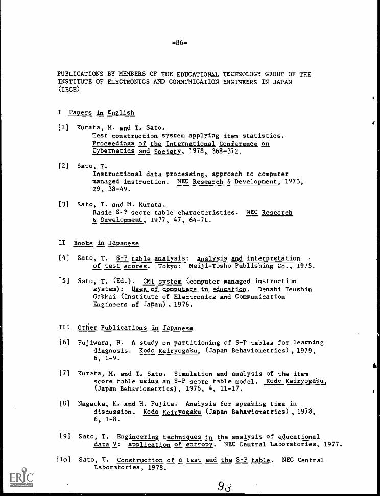
-86-
PUBLICATIONS BY MEMBERS OF THE EDUCATIONAL TECHNOLOGY GROUP OF THEINSTITUTE OF ELECTRONICS AND COMMUNICATION ENGINEERS IN JAPAN(IECE)
I Papers in English
[1] Kurata, M. and T. Sato.Test construction system applying item statistics.Proceedings of the International Conference onCybernetics and Society, 1978, 368-372.
[2] Sato, T.Instructional data processing, approach to computermanaged instruction. NEC Research & Development, 1973,29, 38-49.
[3] Sato, T. and M. Kurata.Basic S-P score table characteristics. NEC Research& Development, 1977, 47, 64-71.
II Books in Japanese
[4] Sato, T. S-P table analysis) Analysis and interpretationof test scores. Tokyo: Meiji-Tosho Publishing Co., 1975.
[5] Sato, T. (Ed.). CMI system (computer managed instructionsystem): Uses d_comouters in education. Denshi TsushinGakkai (Institute of Electronics and CommunicationEngineers of Japan) , 1976.
III Other Publications in Japanese
[6] Fujiwara, H. A study on partitioning of S-F tables for learningdiagnosis. Kodo Keiryogaku, (Japan Behaviometrics) , 1979,6, 1-9.
[7] Kurata, M. and T. Sato. Simulation and analysis of the itemscore table using an S-P score table model. Kodo Keiryogaku,(Japan Behaviometrics), 1976, 4, 11-17.
[8] Nagaoka, K. and H. Fujita. Analysis for speaking time indiscussion. Kodo Keiryogaku (Japan Behaviometrics) , 1978,6, 1-8.
[9] Sato, T. Engineering techniques in the analysis of educationaldata V: application of entropy. NEC Central Laboratories, 1977.
[10] Sato, T. Construction of a test and the S-P table. NEC CentralLaboratories, 1978.
-87-
[11] Sato, T. Hierarchical display of the network of teachingelements using the Interpretive Structural Modelingtechnique. Denshi Tsushin Gakkai (IECE), EducationalTechnology, 1978, 4, 23-28.
[12] Sato, T. How to make and use S-P tables as a method ofanalyzing the test result. Shido to Hyoka (Guidanceand Evaluation), 1978, 282, 44-51.
[13] Sato, T. Item hank system: A set of test items and itscooperative use. Paper presented at the Third Conferenceon Educational Technologies, Naruto, Tokushima, 1978.
[14] Sato, T., M. Kurata and H. Ikeda. Estimation of statisticalcharacteristics of the educational tests. Denshi TsushinGakkai (IECE), Educational Technology, 1978, 2, 27-30.
[15] Sato, T. and H. Chimura. Determination of hierarchicalstructure of instructional units using the InterpretiveStructural Modeling method. Denshi Tsushin Gakkai (IECE),Educational Technology, 1979, I, 11-16.
[16] Takeya, M. and T. Sato. On the learning progress distributionof programmed instruction. Kodo Keiryogaku (JapanBehaviometrics), 1975, 3, 12-21.
[17] Takeya, M. A property analysis of an item score matrixin CHI systems. Trans. IECE, 1977, 60, 967-974.
[18] Takeya, M. Hierarchical structure analysis among instructionalobjectives on student performance scores. DenshiTsushin Gakkai (IECE), Educational Technology, 1978, 7,23-28.
[19] Takeya, M. Application of an item structure analysis to anS-P score table. Denshi Tsushin Gakkai (IECE),Educational Technology, 1978, 12, 35-40.
4
(NI Takeya, M. On an expanded item relational structure analysisand its application. Denshi Tsushin Gakkai (IECE),Educational Technology, 1979, I, 23-26.
[21] Takeya, M. Comparison of the item relational structure analysisbased on it orderliness with other methods. Proceedingsof the Conference of Nippon Kodo Keiryo Gakkai (JapaneseBehaviometric Society), 1979, 102-105.
[22] Takeya, M. Item relational structure analysis based on performancescores for educational evaluation. Trans. IECE, 1979, 62,451-458.
9,;

-88-
(23] Takeya, M. Application of an item relational structure graph
to internal structure analysis of tests. Trans. IECE,
1979, in press.
[24] Yamashita, H., R. Maejima, J. Yokoi, and M. Takeya.
Structure analysis of instructural programs using item
relational structure analysis I. Denshi Tsushin Gakkai
(IECE), Educational Technology, 1979, 1, 27-31.
a U. S. GOVERNMENT PR /WING orrice 1980 u5-641/1973