DOCUMENTATION OF COMPUTER PROGRAM VS2DH FOR SIMULATION OF ENERGY TRANSPORT IN VARIABLY SATURATED POROUS MEDIA--MODIFICA TION OF THE U.S. GEOLOGICAL SURVEY'S COMPUTER PROGRAM VS2DTBy Richard W. Healy and Anne D. Ronan

U.S. GEOLOGICAL SURVEY

Water-Resources Investigations Report 96-4230

Denver, Colorado

1996

U.S. DEPARTMENT OF THE INTERIOR

BRUCE BABBITT, Secretary

U.S. GEOLOGICAL SURVEY

Gordon P. Eaton, Director

The use of trade, product, industry, or firm names is for descriptive purposes only and does not imply endorsement by the U.S. Government.

For additional information write to: Copies of this report can be purchased from:

Chief, Branch of Regional Research U.S. Geological SurveyU.S. Geological Survey Branch of Information ServicesBox 25046, MS 418 Box 25286Denver Federal Center Denver Federal CenterDenver, CO 80225 Denver, CO 80225

CONTENTS

Abstract...........................................................................................................^ 1

Introduction.....................................................................................................^ 1

Theory................. ................................................................................................................................................................... 2

Energy Transport Equation .......................................................................................................................................... 2

Flow Equation.............................................................................................................................................................. 4

Computer Program Structure................................................................................................................................................. 4

Model Verification................................................................................................................................................................... 5

Summary............................................................................................................................................................................... 10

References Cited ............................................................................................................................................... 11

Appendix 1 - Data Input Formats........................................................................................................................................... 13

Appendix 2 - Example Problem Input and Output.................................................................................................................. 26

FIGURES

1. Thermal conductivity of three soils as a function of moisture content (data from van Duin, 1963)............................ 3

2. Results of test problem 2: normalized temperatures as calculated by VS2DH (symbols) and the approximate

analytical solution of Gelharand Collins (1971) (solid line) for times of 250, 500, 1000, and 2000 hours................. 7

3. Soil temperatures for test problem 3 as a function of time as simulated by VS2DH and measured by Jaynes

(1990) for depths of a) 0.1 m; b) 0.2 m; and c) 0.6 m................................................................................................ 9

4. Infiltration rates for test problem 3 as a function of time as simulated by VS2DH and Jaynes (1990) and the

measurements from Jaynes (1990)........................................................................................................................... 10

TABLES

1. Analytical and numerical results for test problem 1.................................................................................................... 6

CONTENTS III

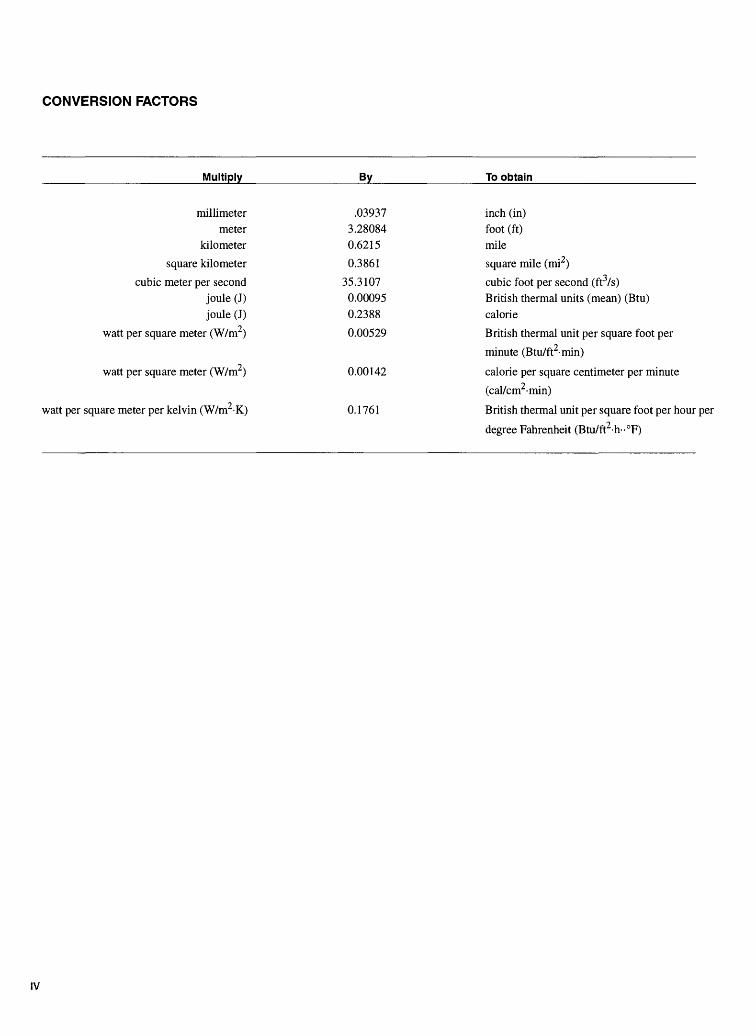
CONVERSION FACTORS

Multiply By To obtain

millimetermeter

kilometer

square kilometer

cubic meter per secondjoule (J)joule (J)

watt per square meter (W/m )

watt per square meter (W/m2)

watt per square meter per kelvin (W/m2 -K)

.039373.280840.6215

0.3861

35.31070.000950.2388

0.00529

0.00142

0.1761

inch (in)foot (ft)mile

square mile (mi2)

cubic foot per second (ft3/s)British thermal units (mean) (Btu)calorie

British thermal unit per square foot per

minute (Btu/ft2-min)

calorie per square centimeter per minute

(cal/cm2-min)

British thermal unit per square foot per hour per

degree Fahrenheit (Btu/ft2 -h-°F)

IV

DOCUMENTATION OF COMPUTER PROGRAM VS2DH FOR SIMULATION OF ENERGY TRANSPORT IN VARIABLY SATURATED POROUS MEDIA- MODIFICATION OF THE U.S. GEOLOGICAL SURVEY'S COMPUTER PROGRAM VS2DTBy Richard W. Healy and Anne D. Ronan

ABSTRACT

This report documents computer program VS2DH for solving problems of energy transport in variably saturated porous media. The program is a modification to the U.S. Geological Survey's computer program VS2DT, which simulates water and solute movement through variably saturated porous media. In VS2DH, the advection-dispersion equation for single phase liquid water is used to describe energy transport. The finite difference method is applied to solve that equation. Regions can be simulated in one or two dimen­ sions. Cartesian or radial coordinates can be used. Three test problems are presented to demonstrate the accuracy of the computer program. In addition, the third test problem serves as an example that allows users to compare results after installation on any computer.

INTRODUCTION

Energy transport can be an important component in a variety of hydrologic and environmental pro­ cesses. Diurnal and annual variations in streamflow loss have been directly linked to diurnal and annual variations in stream water temperature (Lapham, 1989; Constantz and others, 1994). Similarly, strong annual variations in recharge from recharge basins under constant ponding can be attributed to annual water temperature cycles (Nightingale, 1975). Duke (1992) showed that increasing the temperature of irri­ gation water could dramatically increase the rate of infiltration in an agricultural field. Understanding the role of heat flow on these and other processes can be useful in the study and management of water resources.

This report describes computer program VS2DH, which simulates energy transport in porous media under variably saturated conditions. VS2DH assumes a single, constant-density liquid phase flow. Appli­ cations where vapor-phase flow and fluid density variations are negligible are well suited for simulation by VS2DH. Studies where vapor-phase water transport is an important process (such as bare soil evaporation or burial of high-level radioactive waste) would require a model that could account for multiple phases (for example, Milly (1984, 1996)). If variable density liquids are of concern (such as for injection of waste water into a saline aquifer), then models that can account for variable density should be considered (for example, HST 3D (Kipp,1987) or SUTRA (Voss, 1984)).

VS2DH is a modification to the U.S. Geological Survey's computer program VS2DT which simulates water and solute movement under variably saturated conditions. Use of VS2DH requires an awareness of the assumptions and limitations inherent in its development. This report presents a brief description of the­ ory of energy transport and gives details on the numerical implementation of energy transport contained in VS2DH. The energy transport equation is similar to the solute transport equation. As such, there are rela­ tively minor differences between VS2DH and VS2DT (primarily in definitions of parameters that appear in the equations). The descriptions included here are of a somewhat limited scope; before using this program, users should obtain copies of the VS2DT documentations, Lappala and other (1987) and Healy (1990). These references contain necessary information on simulation of water flow and details on parameter defi-

nitions that may not be repeated in this report. To demonstrate the accuracy of VS2DH and illustrate pro­ gram use, three test problems are presented.

THEORY

Energy Transport Equation

The energy transport equation, which is actually a form of the advection-dispersion equation, is derived by balancing the changes in energy stored within a volume of porous media. Such changes occur due to ambient water of different temperature flowing into the volume, thermal conduction into or out of the volume, and energy dispersion into or out of the volume. The energy transport equation can be written with temperature as the dependent variable:

mt [QCW + (l-<t>)CJ T = V-Kj{Q) VT+ V-0 CWDH VT

-VQCw vT+qCw T*; (1)

where / is time in s; 0 is volumetric moisture content; Cw is heat capacity (density times specific heat) of water, in J/m3 °C; <j> is porosity; Cs is heat capacity of the dry solid, in J/m3 °C; Tis temperature, in °C; KT is thermal conductivity of the water and solid matrix (a tensor), in W/m°C; DH is hydrodynamic dispersion tensor, in m2/s; v is water velocity, in m/s; q is rate of fluid source, in s" 1 ; and T* is temperature of fluid source, in °C. Development of Equation (1) ignores the heat capacity of the air phase in the porous medium when moisture content is less than porosity; however, this heat capacity term is small relative to that of water and should therefore be of little practical concern (Sellers, 1965). Further details on Equation (1) can be obtained from Voss (1984) and Kipp (1987).

The left-hand side of Equation (1) represents the change in energy stored in a volume over time. The first term on the right side of the equation describes energy transport by thermal conduction. The second term represents transport due to thermo-mechanical dispersion (Kipp, 1987). The third term on the right side accounts for advective transport of energy. The last term represents heat sources or sinks.

The advective and dispersive components of energy transport are analogous to those in solute trans­ port. Thermo-mechanical dispersion accounts for energy transport as a result of mixing due to the move­ ment of water. The hydrodynamic dispersion tensor is defined as (Healy, 1990):

Dmj = °Jvfiij + (aL - aT)vjVj / Ivl, (2)

where OLT is transverse dispersivity of the porous medium, in m; v,- is the / component of the velocity vec­ tor; 6\y is the Kronecker delta and equals 1 if i=j and otherwise is equal to 0; and OLL is longitudinal disper­ sivity in m; Ivl is magnitude of the velocity vector.

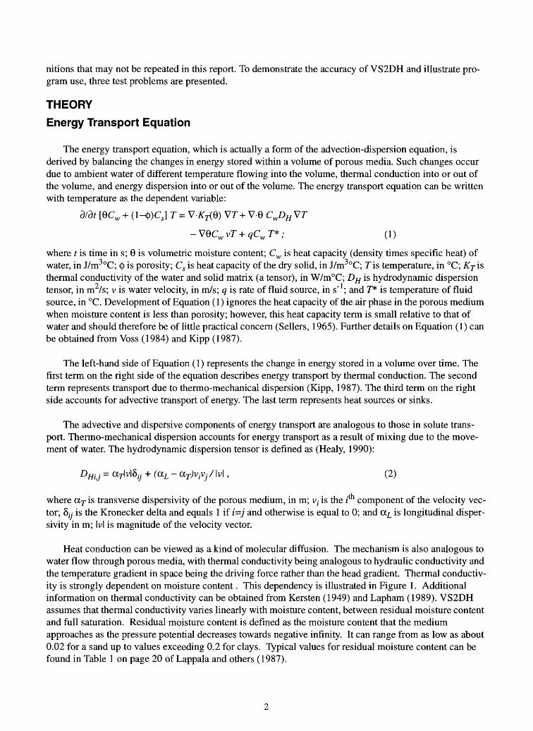
Heat conduction can be viewed as a kind of molecular diffusion. The mechanism is also analogous to water flow through porous media, with thermal conductivity being analogous to hydraulic conductivity and the temperature gradient in space being the driving force rather than the head gradient. Thermal conductiv­ ity is strongly dependent on moisture content. This dependency is illustrated in Figure 1. Additional information on thermal conductivity can be obtained from Kersten (1949) and Lapham (1989). VS2DH assumes that thermal conductivity varies linearly with moisture content, between residual moisture content and full saturation. Residual moisture content is defined as the moisture content that the medium approaches as the pressure potential decreases towards negative infinity. It can range from as low as about 0.02 for a sand up to values exceeding 0.2 for clays. Typical values for residual moisture content can be found in Table 1 on page 20 of Lappala and others (1987).

0.1 0.2 0.3 0.4 0.5 volumetric moisture content, dimensionless

Figure 1. Thermal conductivity of three soils as a function of moisture content (data from van Duin, 1963).

Advection accounts for energy transport by the movement of water of different temperatures. As such, the mechanism is identical to that for solute transport.

Source/sink terms account for energy introduced to or removed from the domain by the movement of water into or out of the domain. These terms are represented by the last term in equation (1). Typically these take the form of injection or withdrawal wells.

Boundaries can be assigned as fixed heat fluxes or fixed temperature. In addition, the temperature of any inflowing water from a fluid-flow boundary must be specified. When water flows out of the domain through a flow boundary, the program sets the temperature of that water equal to the temperature in the finite difference cell where the water is exiting.

Flow Equation

The flow equation solved by VS2DH is identical to that given by Equation 9 on page 7 of Lappala and others (1987) with one exception. Because of the temperature dependency of viscosity, saturated hydraulic conductivity, K, is now treated as a function of temperature:

(3)on n

where p is density, in kg/m ; g is gravity, in m/s ; k is intrinsic permeability, in m ; and \JL is viscosity, in Ns/m2 . Viscosity is calculated according to the empirical formula (Kipp, 1987):

\i(T) = 0.00002414 x io[247- 8/(T+133J6)] (4)

Although the density of water is also dependent on temperature, it is treated as a constant in VS2DH because its dependence is much less than that of viscosity over the range of pore-water pressures and tem­ peratures typically encountered under variably saturated field conditions.

The van Genuchten equations are used to represent moisture content, specific moisture capacity, and relative hydraulic conductivity as functions of pressure head. Use of alternate equations is described in Lappala and others (1987).

COMPUTER PROGRAM STRUCTURE

Development of VS2DH required substantial modification to subroutine VTSETUP in VS2DT, minor modifications to VSEXEC, and the addition of function subroutine THERMC for calculating thermal con­ ductivity as a function of volumetric moisture content. A copy of the FORTRAN version of the program can be obtained from the address shown on page ii.

The revised structure of the program requires that three new global variables be introduced: NITS, EPS2, and VMAX, whose values are explained in the following sentences. Because temperature is a vari­ able within both the flow and transport equations, the two equations could be solved simultaneously. How­ ever, VS2DT is set up to solve the equations sequentially. VS2DH maintains the sequential solution algorithm, necessitating iterative solution of both equations within each time step. The flow equation is solved first, assuming a temperature equal to that at the previous time step. Next the transport equation is solved to update the value of temperature. The flow equation is then resolved with the updated tempera­ ture. This iterative process is continued within the time step until the change in velocity between subse­ quent solutions of the flow equation (VMAX) is less in magnitude than EPS2 at every node. The total number of iterations is NITS. Experience has shown that NITS rarely exceeds a value of 4 or 5. At the com­ pletion of every time step, the energy flux into and out of the system, as well as the change in energy stored in the system is calculated in subroutine VSFLUX.

A few options pertaining to solute transport that were available in VS2DT are not allowed in VS2DH. These include solute decay, adsorption, and cation exchange. The user is also cautioned against using the bare soil evaporation or plant transpiration options without careful analysis. These processes are in reality highly temperature dependent, but the program does not treat them as such.

Input-data formats are described in Appendix 1. The formats are quite similar to those in VS2DT (Healy, 1990). A value is now required for EPS2 and the definitions of several of the parameters contained in array HT are modified. Also, SI units must now be used for all data; time must be in seconds, length in meters, temperature in degrees Centigrade, and mass in kilograms. The program assumes a reference tem­ perature of 20°C. Input data values for saturated hydraulic conductivity should correspond to this refer-

ence temperature.

MODEL VERIFICATION

Three problems are presented to evaluate the accuracy of the new program. In addition the third test problem also serves as an example that allows users to compare program output after installation on any computer.

One-Dimensional Saturated Flow and Heat Transport Problem

This test problem simulates heated water flowing into a one-dimensional saturated column of cool water. It is intended to demonstrate the ability of VS2DH to match an analytical solution to a hypothetical laboratory experiment. The problem is based on example problem 6 presented in documentation for the U.S. Geological Survey computer program HST3D (Kipp, 1987, p. 244). Model parameters are:

£=1.389xl(r4 m/s;

(|> = 0 = 0.50;

OLL = OLT = 10 m;

Cs = 2.08xl06 J/m3°C;

Cw = 4.2xl06 J/m3°C;

Initial column temperature T0 = 20°C; and

Influent water temperature Tinj = 21°C.

An interstitial velocity of 2.778x1 0"4 m/s was imposed through the column by orienting the column in a vertical direction and specifying a constant pressure head boundary condition of 1 m at each end of the column.

The domain was modeled using a series of increasingly finer discretizations in both space and time. The discretization was centered in space and time. With a spatial discretization of 1.0 m and a time discret­ ization of 107.65 s (approximately 0.03 hr), the temperatures predicted by VS2DH were in very close agreement with the analytical solution of Ogata and Banks (1961). Table 1 compares normalized tempera­ tures predicted by VS2DH to the analytical solution at a time of 10765 s.

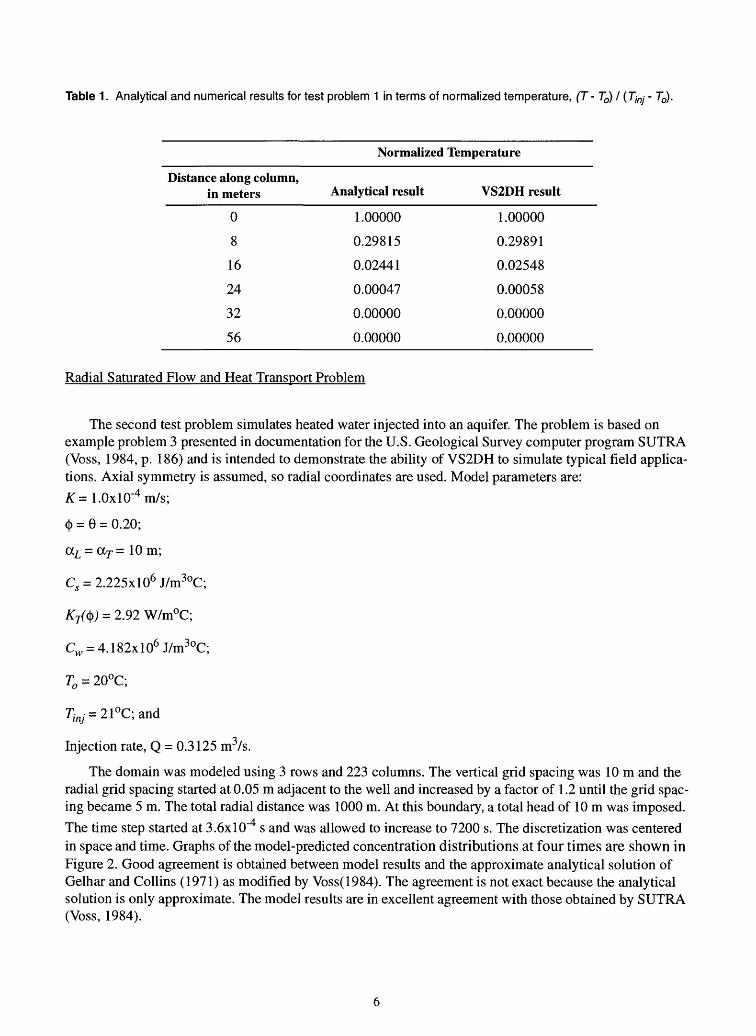
Table 1. Analytical and numerical results for test problem 1 in terms of normalized temperature, (T- T0) I (7/ny - T0).

Normalized Temperature

Distance along column,in meters Analytical result VS2DH result

0

8

16

24

32

56

1.00000

0.29815

0.02441

0.00047

0.00000

0.00000

1.00000

0.29891

0.02548

0.00058

0.00000

0.00000

Radial Saturated Flow and Heat Transport Problem

The second test problem simulates heated water injected into an aquifer. The problem is based on example problem 3 presented in documentation for the U.S. Geological Survey computer program SUTRA (Voss, 1984, p. 186) and is intended to demonstrate the ability of VS2DH to simulate typical field applica­ tions. Axial symmetry is assumed, so radial coordinates are used. Model parameters are:£=1.0xlO-4 m/s;

<j> = 6 = 0.20;

aL = aT = 10 m;

Cs = 2.225xl06 J/m3°C;

Krfty) = 2.92 W/m°C;

Cw = 4.182xl06 J/m3 °C;

T0 = 20°C;

Tinj = 21°C; and

Injection rate, Q = 0.3125 m3/s.

The domain was modeled using 3 rows and 223 columns. The vertical grid spacing was 10 m and the radial grid spacing started at 0.05 m adjacent to the well and increased by a factor of 1.2 until the grid spac­ ing became 5 m. The total radial distance was 1000 m. At this boundary, a total head of 10 m was imposed.The time step started at 3.6x10 s and was allowed to increase to 7200 s. The discretization was centered in space and time. Graphs of the model-predicted concentration distributions at four times are shown in Figure 2. Good agreement is obtained between model results and the approximate analytical solution of Gelhar and Collins (1971) as modified by Voss(1984). The agreement is not exact because the analytical solution is only approximate. The model results are in excellent agreement with those obtained by SUTRA (Voss, 1984).

0 100 200 300 400

RADIAL DISTANCE, IN METERS

500

Figure 2. Results of test problem 2: normalized temperatures as calculated by VS2DH (symbols) and the approximate analytical solution of Gelhar and Collins (1971).

One-Dimensional Ponded Infiltration with Time-Varying (Diurnal) Temperature

This test problem simulates one-dimensional flow of water in the unsaturated zone in response to a ponded surface that experiences diurnal temperature fluctuations. The problem is constructed to replicate the field conditions reported by Jaynes (1990). In brief, Jaynes monitored depth of ponding, inflows required to maintain ponding, temperature of ponded water, and temperature of moist sediments at three depths below the ground surface. From the ponding depths and inflows, he determined infiltration rates. In an effort to qualitatively determine if daily temperature changes in the ponded water could explain the vari­ ation in infiltration, he used a simplified finite-difference approximation of the governing equations to sim­ ulate the problem. His calibration procedure consisted of varying the hydraulic conductivity of the

sediments. Properties of the sediments were not measured.

Jaynes (1990) found that he needed to simulate a lower hydraulic conductivity surface crust to ade­ quately simulate the infiltration rates. He set the hydraulic conductivity of the surface crust tol/20 of that of the underlying sediments. Lacking complete description of the soil unsaturated characteristic curves, we assigned soil properties of the Columbia Sandy Loam (Laliberte and others, 1966, table C-5). We found that we needed to set K for the surface crust to 1/200 of that of the underlying sediments (probably because we did not use the same characteristic curves as Jaynes, 1990). Model parameters are:

K = 4.0x1 0"8 m/s for the surface crust;

K = 8.0x1 0"6 m/s for the underlying sediments;

<1> = 0.496;

OLL = ar = 0.01 m;

C, = 2.18xl06 J/m3 °C;

CM, = 4.18xl06 J/m3 °C.

The domain was modeled in one dimension using 3 columns and 129 rows. The vertical grid spacing varied from 0.001 m at the surface to 0.5 m at depth. The total domain depth was 49.6 m from the ground surface to the water table. The total simulation time was 168 hours, consisting of 168 one-hour recharge periods. The timestep started at 360 s and was allowed to increase to 3600 s. The discretization was cen­ tered in space and in time.

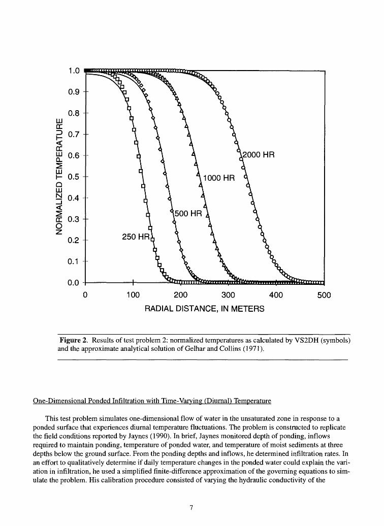
For the entire simulation, the flow equation boundary conditions were a specified total head of 0.04 m at the ground surface (the average depth of ponded water) and a specified pressure head of zero at the water table. The energy equation boundary conditions consisted of specified temperatures at the ground surface and at the water table. The temperature at the water table was held constant at 21.3°C while the specified surface temperatures were changed every hour. The first 60 hours of the simulation were a start-up period, using a repeated cyclic temperature pattern at the surface. For the subsequent 108 hours of the simulation, Jaynes (1990) measured pond temperatures were used as the surface boundary condition.

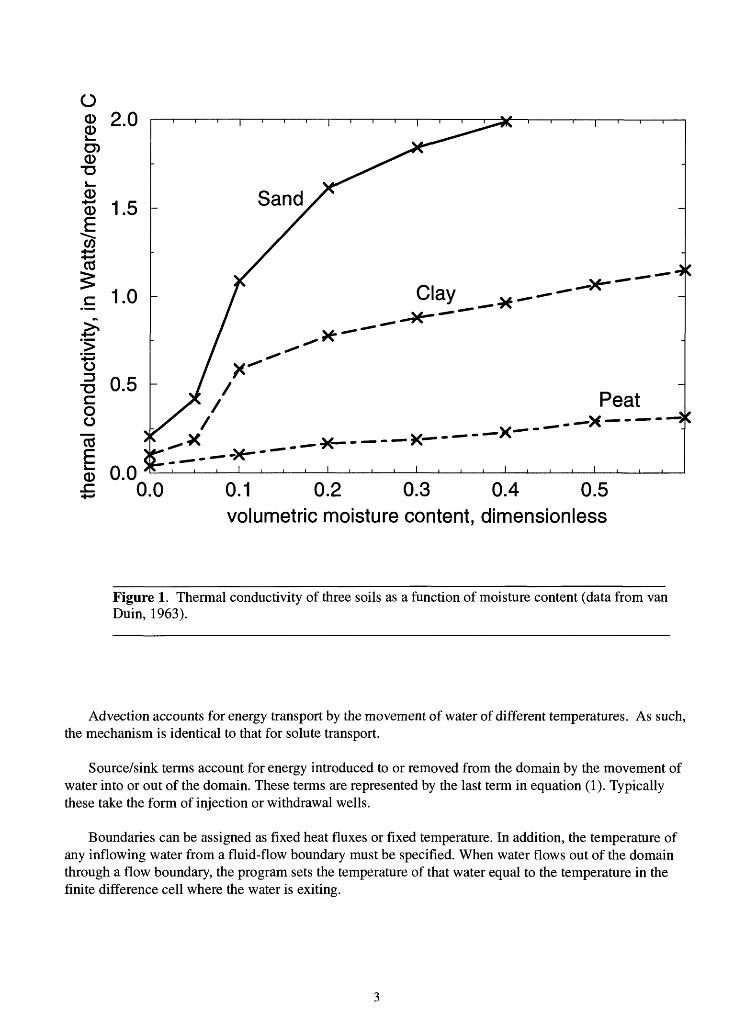
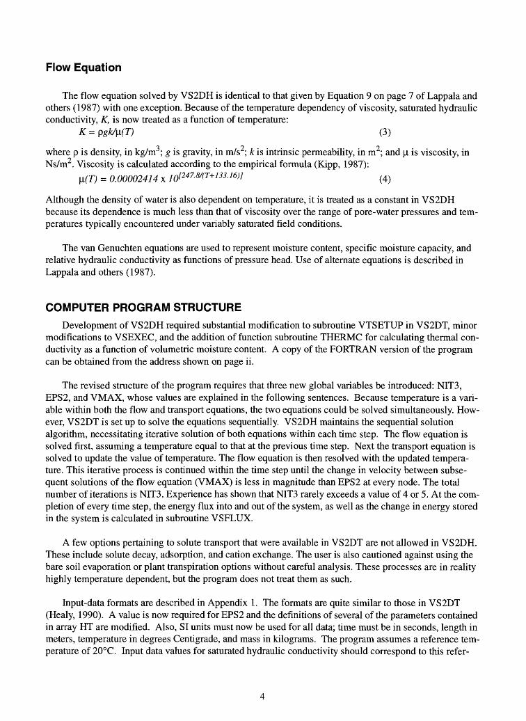
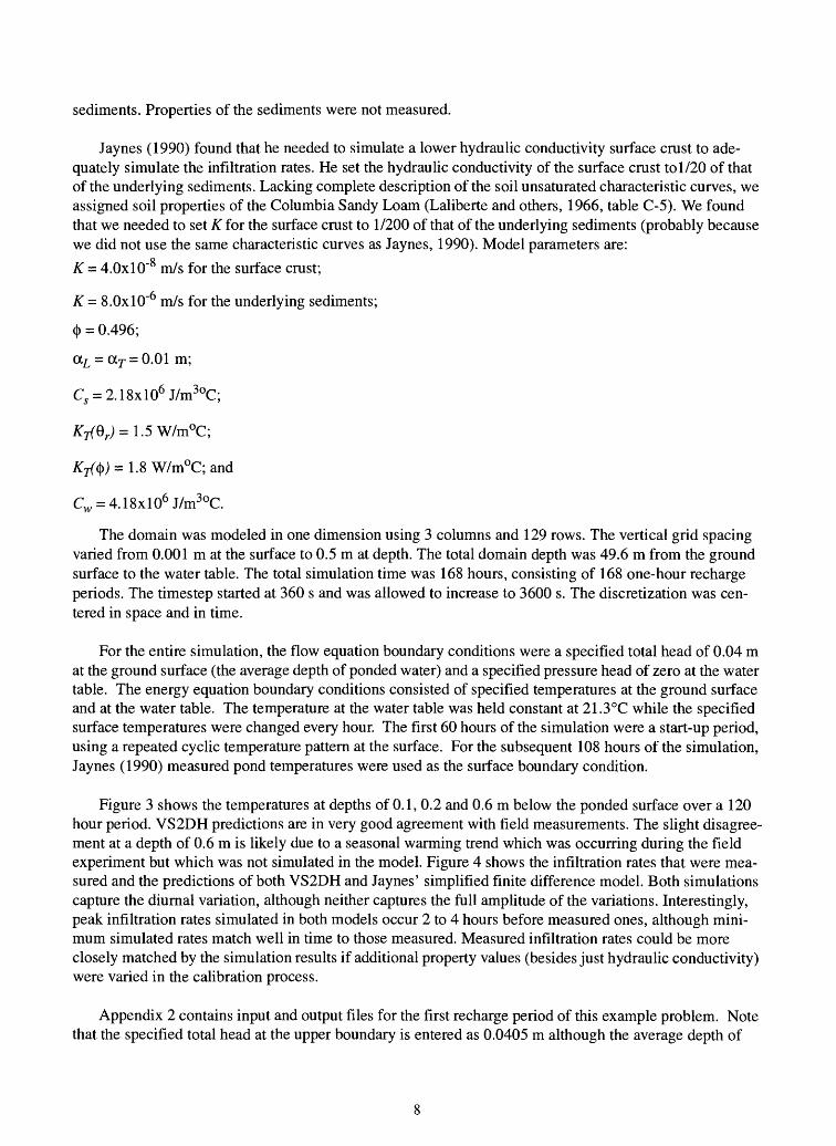
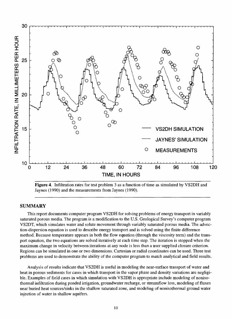
Figure 3 shows the temperatures at depths of 0.1, 0.2 and 0.6 m below the ponded surface over a 120 hour period. VS2DH predictions are in very good agreement with field measurements. The slight disagree­ ment at a depth of 0.6 m is likely due to a seasonal warming trend which was occurring during the field experiment but which was not simulated in the model. Figure 4 shows the infiltration rates that were mea­ sured and the predictions of both VS2DH and Jaynes' simplified finite difference model. Both simulations capture the diurnal variation, although neither captures the full amplitude of the variations. Interestingly, peak infiltration rates simulated in both models occur 2 to 4 hours before measured ones, although mini­ mum simulated rates match well in time to those measured. Measured infiltration rates could be more closely matched by the simulation results if additional property values (besides just hydraulic conductivity) were varied in the calibration process.

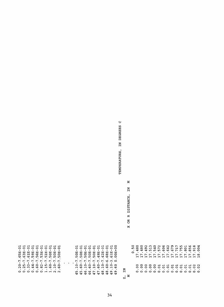
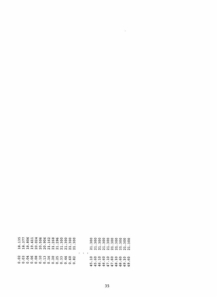
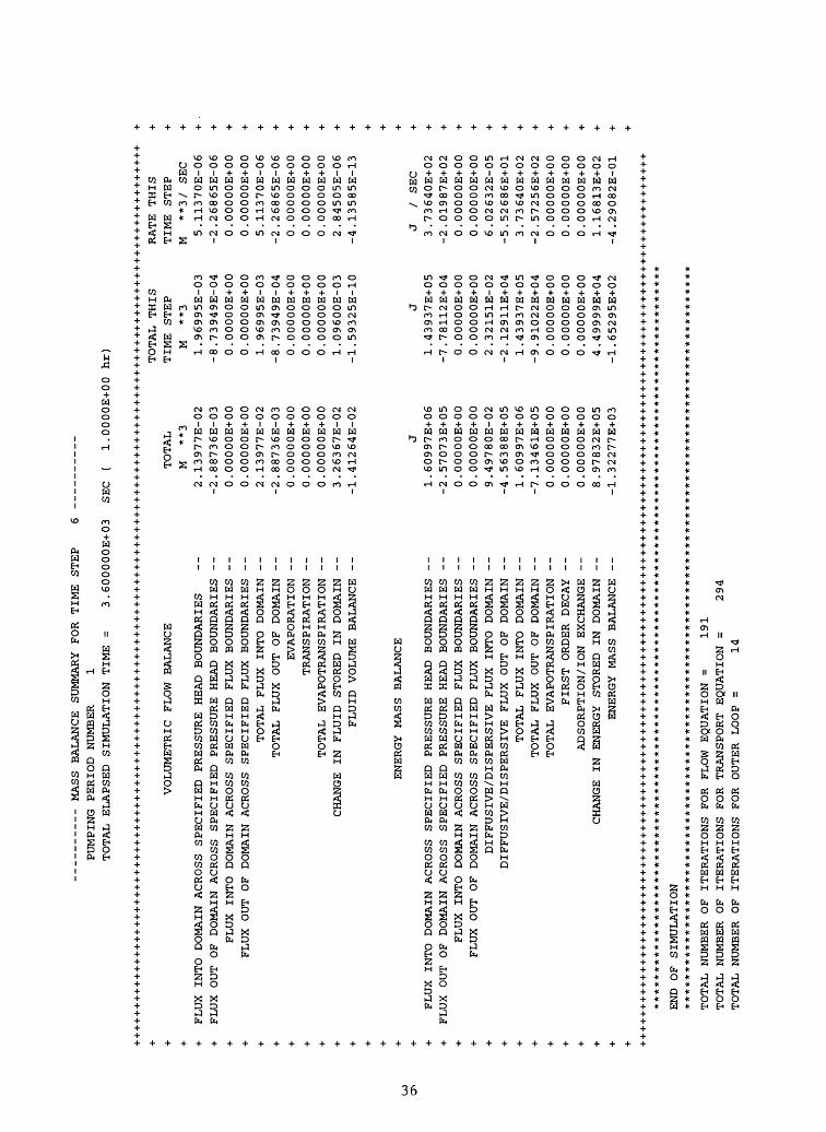
Appendix 2 contains input and output files for the first recharge period of this example problem. Note that the specified total head at the upper boundary is entered as 0.0405 m although the average depth of

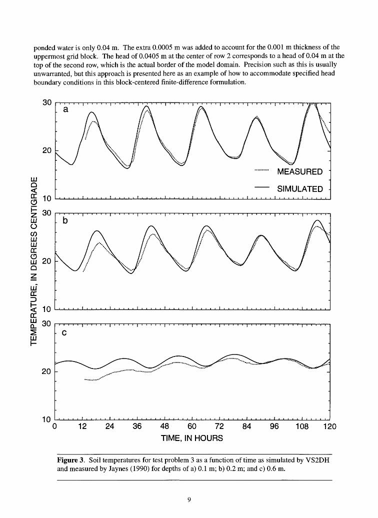
ponded water is only 0.04 m. The extra 0.0005 m was added to account for the 0.001 m thickness of the uppermost grid block. The head of 0.0405 m at the center of row 2 corresponds to a head of 0.04 m at the top of the second row, which is the actual border of the model domain. Precision such as this is usually unwarranted, but this approach is presented here as an example of how to accommodate specified head boundary conditions in this block-centered finite-difference formulation.

LU Q

Q_^ LLJ

30

20

10

MEASURED

SIMULATED

30LUoCO LU LLJ DC

S20Q

LLJ DC

< 10DCLLJ 30

20

100 12 24 36 48 60 72 84

TIME, IN HOURS

96 108 120

Figure 3. Soil temperatures for test problem 3 as a function of time as simulated by VS2DH and measured by Jaynes (1990) for depths of a) 0.1 m; b) 0.2 m; and c) 0.6 m.

30

cnD OIcnLJJQL 25 COcnLJJ

LJJ

2 20zUJ

cnz

cn

EEz

10

VS2DH SIMULATION

JAYNES' SIMULATION

MEASUREMENTS

0 12 24 36 48 60 72

TIME, IN HOURS

84 96 108 120

Figure 4. Infiltration rates for test problem 3 as a function of time as simulated by VS2DH and Jaynes (1990) and the measurements from Jaynes (1990).

SUMMARY

This report documents computer program VS2DH for solving problems of energy transport in variably saturated porous media. The program is a modification to the U.S. Geological Survey's computer program VS2DT, which simulates water and solute movement through variably saturated porous media. The advec- tion-dispersion equation is used to describe energy transport and is solved using the finite difference method. Because temperature appears in both the flow equation (through the viscosity term) and the trans­ port equation, the two equations are solved iteratively at each time step. The iteration is stopped when the maximum change in velocity between iterations at any node is less than a user supplied closure criterion. Regions can be simulated in one or two dimensions. Cartesian or radial coordinates can be used. Three test problems are used to demonstrate the ability of the computer program to match analytical and field results.

Analysis of results indicate that VS2DH is useful in modeling the near-surface transport of water and heat in porous sediments for cases in which transport in the vapor phase and density variations are negligi­ ble. Examples of field cases in which simulation with VS2DH is appropriate include modeling of noniso- thermal infiltration during ponded irrigation, groundwater recharge, or streamflow loss, modeling effluxes near buried heat sources/sinks in the shallow saturated zone, and modeling of nonisothermal ground water injection of water in shallow aquifers.

10

REFERENCES

Constantz, Jim, Thomas, C.L., and Zellweger, Gary, 1994, Influence of diurnal variations in stream tem­ perature on streamflow loss and groundwater recharge: Water Resources Research, v. 30, no. 12, p.3253-3264.

Duke, H.R., 1992, Water temperature fluctuations and effect on irrigation infiltration: Transactions of the American Society of Agricultural Engineers, v. 35, no. 1, p. 193-199.

Gelhar, L.W, and Collins, M.A., 1971, General analysis of longitudinal dispersion in nonuniform flow: Water Resources Research, v. 7, no. 6, p. 1511-1521.

Healy, R.W, 1990, Simulation of solute transport in variably saturated porous media with supplementalinformation on modifications to the U.S. Geological Survey's computer program VS2D: U.S. Geo­ logical Survey Water-Resources Investigations Report 90-4025, 125 p.

Jaynes, D.B., 1990, Temperature variations effect on field-measured infiltration: Soil Science Society of America Journal, v. 54, no. 2, p. 305-311.

Kersten, M.S., 1949, Thermal properties of soils: University of Minnesota Engineering Experiment Station Bulletin 28, approx. 225 p.

Kipp, K.L., 1987, HST3D: A computer code for simulation of heat and solute transport inthree-dimensional ground-water flow systems: U.S. Geological Survey Water-Resources Investi­ gations Report 86-4095, 517 p.

Laliberte, G.E., Corey, A.T., and Brooks, R.H., 1966, Properties of unsaturated porous media: Fort Collins, Colorado State University Hydrology Paper 17, 40 p.

Lapham, WW, 1989, Use of temperature profiles beneath streams to determine rates of vertical ground water flow and vertical hydraulic conductivity: U.S. Geological Survey Water-Supply Paper 2337, 35 p.

Lappala, E.G., Healy, R.W, and Weeks, E.P., 1987, Documentation of computer program VS2D to solve the equations of fluid flow in variably saturated porous media: U.S. Geological Survey Water- Resources Investigations Report 83-4099, 184 p.

Milly, P.C.D., 1984, A simulation analysis of thermal effects on evaporation from soil: Water Resources Research, v. 20, no. 8, p. 1087-1098.

Milly, P.C.D., 1996, Effects of thermal vapor diffusion on seasonal dynamics of water in the unsaturated zone: Water Resources Research, v. 32, no. 3, p. 509-518.

Nightingale, H.I., 1975, Groundwater recharge rates from thermometry: Groundwater, v.13, p. 340-344.

Ogata, Akio, and Banks, R.B., 1961, A solution of the differential equation of longitudinal dispersion in porous media: U.S. Geological Survey Professional Paper 411-A, 7 p.

11

Sellers, W.D., 1965, Physical Climatology: University of Chicago Press, 272 p.

van Duin, R.H.A.,1963, The influence of management on the temperature wave near the surface: Wagenin- gen, Institute for Land and Water Management Research, Technical Bulletin 29.

Voss, C.I., 1984, A finite-element simulation model for saturated-unsaturated, fluid-density-dependent ground-water flow with energy transport or chemically reactive single-species solute transport: U.S. Geological Survey Water-Resources Investigations Report 84-4369, 409 p.

12

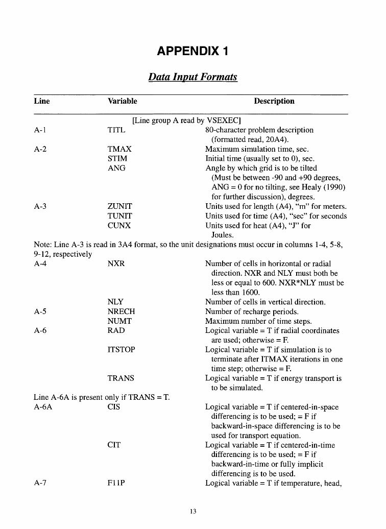
APPENDIX 1

Data Input Formats

Line Variable Description

[Line group A read by VSEXEC] A-l TITL 80-character problem description

(formatted read, 20A4).A-2 TMAX Maximum simulation time, sec.

STIM Initial time (usually set to 0), sec. ANG Angle by which grid is to be tilted

(Must be between -90 and +90 degrees, ANG = 0 for no tilting, see Healy (1990) for further discussion), degrees.

A-3 ZUNIT Units used for length (A4), "m" for meters.TUNIT Units used for time (A4), "sec" for seconds CUNX Units used for heat (A4), "J" for

Joules.Note: Line A-3 is read in 3A4 format, so the unit designations must occur in columns 1-4, 5-8, 9-12, respectivelyA-4 NXR Number of cells in horizontal or radial

direction. NXR and NLY must both be less or equal to 600. NXR*NLY must be less than 1600.

NLY Number of cells in vertical direction. A-5 NRECH Number of recharge periods.

NUMT Maximum number of time steps. A-6 RAD Logical variable = T if radial coordinates

are used; otherwise = F. ITSTOP Logical variable = T if simulation is to

terminate after ITMAX iterations in one time step; otherwise = F.

TRANS

Line A-6A is present only if TRANS = T. A-6A CIS

CIT

A-7 F11P

Logical variable = T if energy transport is to be simulated.

Logical variable = T if centered-in-space differencing is to be used; = F if backward-in-space differencing is to be used for transport equation.

Logical variable = T if centered-in-time differencing is to be used; = F if backward-in-time or fully implicit differencing is to be used.

Logical variable = T if temperature, head,

13

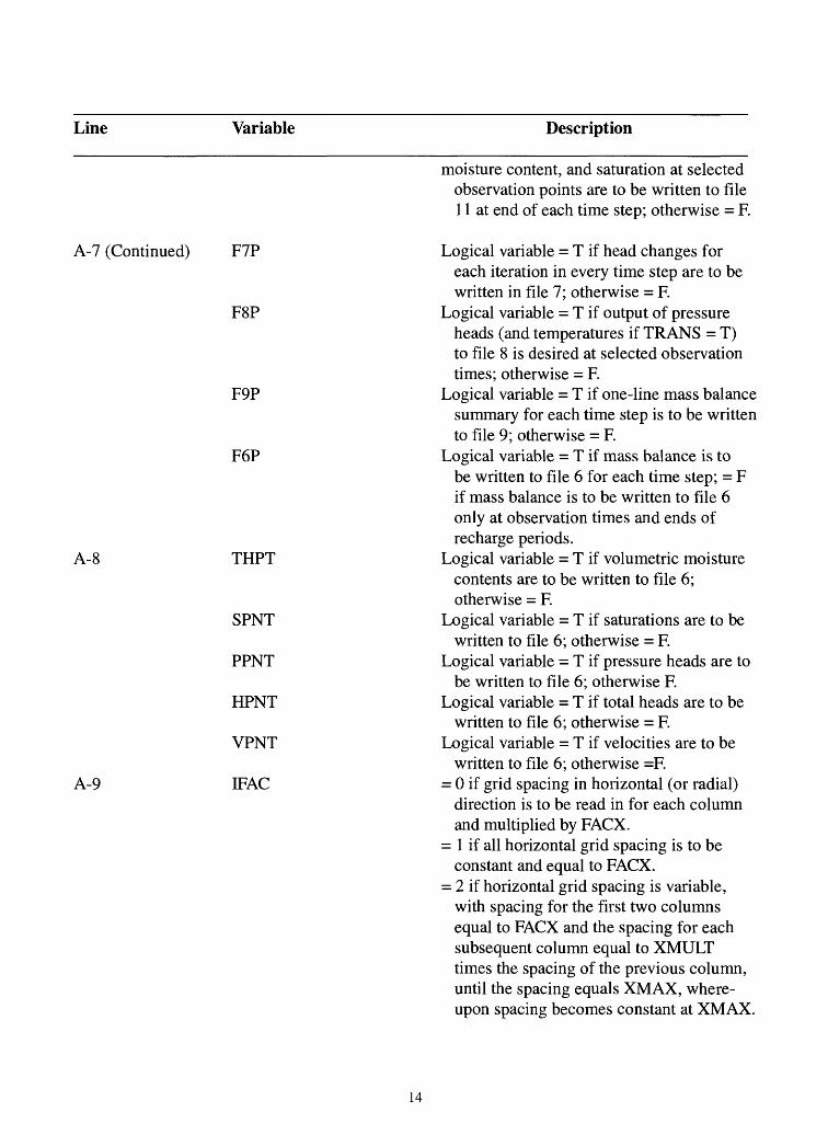
Line Variable Description

A-7 (Continued) FTP

F8P

F9P

F6P

A-8

A-9

THPT

SPNT

PPNT

HPNT

VPNT

IFAC

moisture content, and saturation at selected observation points are to be written to file 11 at end of each time step; otherwise = F.

Logical variable = T if head changes for each iteration in every time step are to be written in file 7; otherwise = F

Logical variable = T if output of pressure heads (and temperatures if TRANS = T) to file 8 is desired at selected observation times; otherwise = F.

Logical variable = T if one-line mass balance summary for each time step is to be written to file 9; otherwise = F.

Logical variable = T if mass balance is to be written to file 6 for each time step; = F if mass balance is to be written to file 6 only at observation times and ends of recharge periods.

Logical variable = T if volumetric moisture contents are to be written to file 6; otherwise = F.

Logical variable = T if saturations are to be written to file 6; otherwise = F

Logical variable = T if pressure heads are to be written to file 6; otherwise F.

Logical variable = T if total heads are to be written to file 6; otherwise = F

Logical variable = T if velocities are to be written to file 6; otherwise =F

= 0 if grid spacing in horizontal (or radial) direction is to be read in for each column and multiplied by FACX.

= 1 if all horizontal grid spacing is to be constant and equal to FACX.

= 2 if horizontal grid spacing is variable, with spacing for the first two columns equal to FACX and the spacing for each subsequent column equal to XMULT times the spacing of the previous column, until the spacing equals XMAX, where­ upon spacing becomes constant at XMAX.

14

Line Variable Description

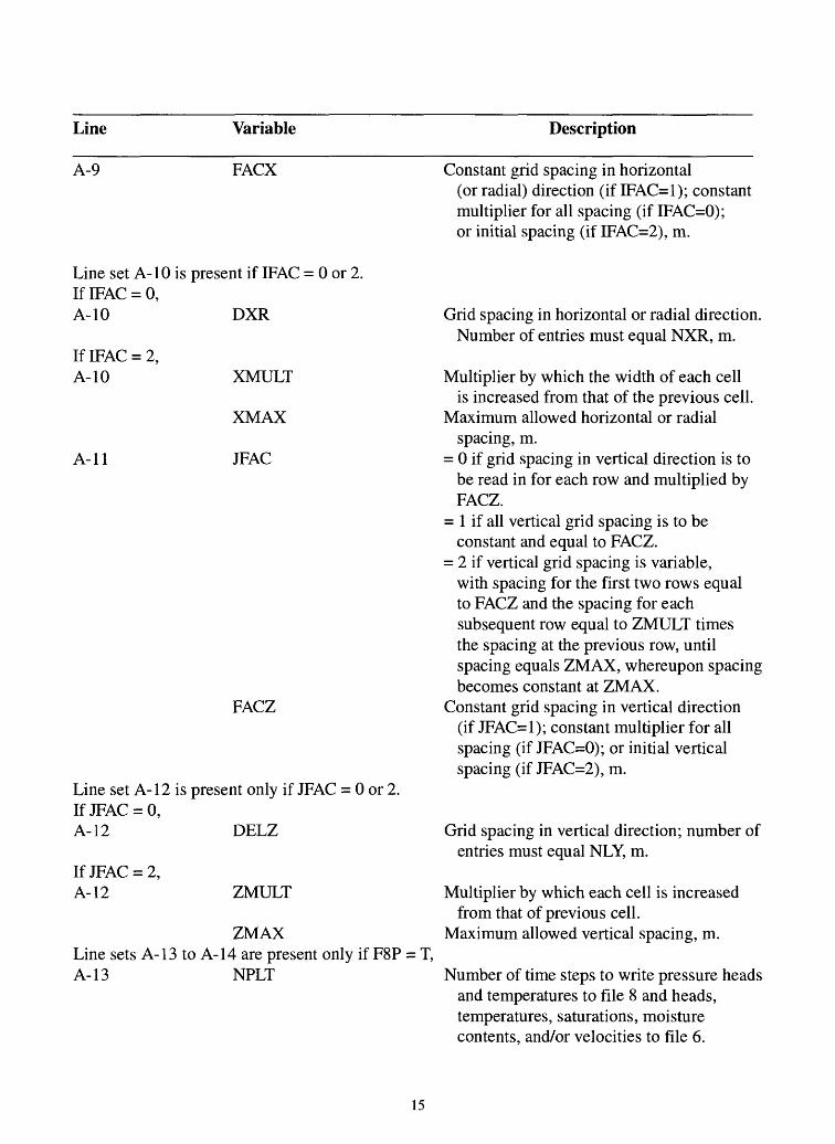
A-9 FACX

Line set A-10 is present if IFAC = 0 or 2.IfIFAC = 0,A-10 DXR

If IFAC = 2, A-10

A-ll

XMULT

XMAX

JFAC

FACZ

Line set A-12 is present only if JFAC = 0 or 2.If JFAC = 0,A-12 DELZ

If JFAC = 2, A-12 ZMULT

ZMAXLine sets A-13 to A-14 are present only if F8P A-13 NPLT

= T,

Constant grid spacing in horizontal (or radial) direction (if IFAC=1); constant multiplier for all spacing (if IFAC=0); or initial spacing (if IFAC=2), m.

Grid spacing in horizontal or radial direction. Number of entries must equal NXR, m.

Multiplier by which the width of each cell is increased from that of the previous cell.

Maximum allowed horizontal or radial spacing, m.

= 0 if grid spacing in vertical direction is to be read in for each row and multiplied by FACZ.

= 1 if all vertical grid spacing is to be constant and equal to FACZ.

= 2 if vertical grid spacing is variable, with spacing for the first two rows equal to FACZ and the spacing for each subsequent row equal to ZMULT times the spacing at the previous row, until spacing equals ZMAX, whereupon spacing becomes constant at ZMAX.

Constant grid spacing in vertical direction (if JFAC=1); constant multiplier for all spacing (if JFAC=0); or initial vertical spacing (if JFAC=2), m.

Grid spacing in vertical direction; number of entries must equal NLY, m.

Multiplier by which each cell is increasedfrom that of previous cell.

Maximum allowed vertical spacing, m.

Number of time steps to write pressure heads and temperatures to file 8 and heads, temperatures, saturations, moisture contents, and/or velocities to file 6.

15

Line Variable Description

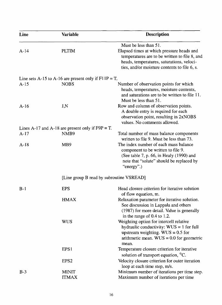
A-14 PLTIMMust be less than 51.

Elapsed times at which pressure heads and temperatures are to be written to file 8, and heads, temperatures, saturations, veloci­ ties, and/or moisture contents to file 6, s.

Line sets A-15 to A-16 are present only if Fl IP = T,A-15

A-16

NOBS

J,N

Lines A-17 and A-18 are present only if F9P = T. A-17 NMB9

A-18 MB9

Number of observation points for which heads, temperatures, moisture contents, and saturations are to be written to file 11. Must be less than 51.

Row and column of observation points. A double entry is required for each observation point, resulting in 2xNOBS values. No comments allowed.

Total number of mass balance components written to file 9. Must be less than 73.

The index number of each mass balance component to be written to file 9. (See table 7, p. 66, in Healy (1990) and note that "solute" should be replaced by "energy".)

[Line group B read by subroutine VSREAD]

B-l EPS

HMAX

WUS

B-3

EPS1

EPS2

MINIT ITMAX

Head closure criterion for iterative solutionof flow equation, m.

Relaxation parameter for iterative solution.See discussion in Lappala and others(1987) for more detail. Value is generallyin the range of 0.4 to 1.2.

Weighting option for intercell relativehydraulic conductivity: WUS = 1 for fullupstream weighting. WUS = 0.5 forarithmetic mean. WUS = 0.0 for geometricmean.

Temperature closure criterion for iterativesolution of transport equation, °C.

Velocity closure criterion for outer iterationloop at each time step, m/s.

Minimum number of iterations per time step. Maximum number of iterations per time

16

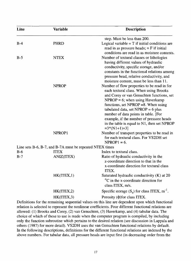
Line Variable Description

step. Must be less than 200.B-4 PHRD Logical variable = T if initial conditions are

read in as pressure heads; = F if initial conditions are read in as moisture contents.

B-5 NTEX Number of textural classes or lithologieshaving different values of hydraulic conductivity, specific storage, and/or constants in the functional relations among pressure head, relative conductivity, and moisture content, must be less than 11.

NPROP Number of flow properties to be read in foreach textural class. When using Brooks and Corey or van Genuchten functions, set NPROP = 6; when using Haverkamp functions, set NPROP =8. When using tabulated data, set NPROP = 6 plus number of data points in table. [For example, if the number of pressure heads in the table is equal to Nl, then set NPROP =3*(Nl+l)+3]

NPROP 1 Number of transport properties to be read infor each textural class. For VS2DH set NPROP1 = 6.

Line sets B-6, B-7, and B-7A must be repeated NTEX timesB-6 ITEX Index to textural class.B-7 ANIZ(ITEX) Ratio of hydraulic conductivity in the

z-coordinate direction to that in the x-coordinate direction for textural class ITEX.

HK(ITEX, 1) Saturated hydraulic conductivity (K) at 20°C in the x-coordinate direction for class ITEX, m/s.

HK(ITEX,2) Specific storage (Ss) for class ITEX, m" 1 .

HK(ITEX,3) Porosity (<|))for class ITEX.Definitions for the remaining sequential values on this line are dependent upon which functional relation is selected to represent the nonlinear coefficients. Four different functional relations are allowed: (1) Brooks and Corey, (2) van Genuchten, (3) Haverkamp, and (4) tabular data. The choice of which of these to use is made when the computer program is compiled, by including only the function subroutine which pertains to the desired relation (see discussion in Lappala and others (1987) for more detail). VS2DH uses the van Genuchten functional relations by default. In the following descriptions, definitions for the different functional relations are indexed by the above numbers. For tabular data, all pressure heads are input first (in decreasing order from the

17

Line Variable Description

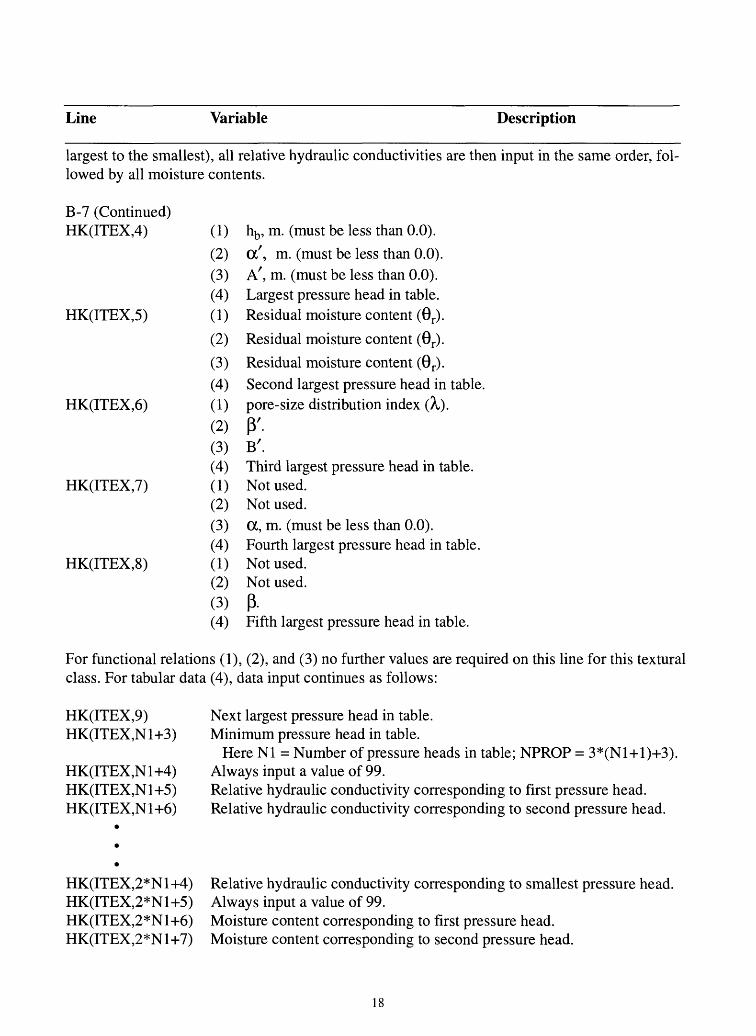
largest to the smallest), all relative hydraulic conductivities are then input in the same order, fol­ lowed by all moisture contents.

B-7 (Continued) HK(ITEX,4)

HK(ITEX,5)

(1) h^, m. (must be less than 0.0).

(2) a', m. (must be less than 0.0).(3) A', m. (must be less than 0.0).(4) Largest pressure head in table.(1) Residual moisture content (0r).

(2) Residual moisture content (0r).

(3) Residual moisture content (0r).(4) Second largest pressure head in table.(1) pore-size distribution index (A,).(2) P'.(3) B'.(4) Third largest pressure head in table.(1) Not used.(2) Not used.(3) a, m. (must be less than 0.0).(4) Fourth largest pressure head in table.(1) Not used.(2) Not used.(3) PL(4) Fifth largest pressure head in table.

For functional relations (1), (2), and (3) no further values are required on this line for this textural class. For tabular data (4), data input continues as follows:

HK(ITEX,6)

HK(ITEX,7)

HK(ITEX,8)

HK(ITEX,9) HK(ITEX,Nl+3)

HK(ITEX,Nl+4) HK(ITEX,Nl+5) HK(ITEX,Nl+6)

Next largest pressure head in table. Minimum pressure head in table.

Here Nl = Number of pressure heads in table; NPROP = 3*(Nl+l)+3). Always input a value of 99.Relative hydraulic conductivity corresponding to first pressure head. Relative hydraulic conductivity corresponding to second pressure head.

HK(ITEX,2*Nl+4) Relative hydraulic conductivity corresponding to smallest pressure head.HK(ITEX,2*Nl+5) Always input a value of 99.HK(ITEX,2*Nl+6) Moisture content corresponding to first pressure head.HK(ITEX,2*Nl+7) Moisture content corresponding to second pressure head.

18

Line Variable Description

B-7 (Continued)HK(ITEX,3*Nl+5) Moisture content corresponding to smallest pressure head.HK(ITEX,3*Nl+6) Always input a value of 99.Regardless of which functional relation is selected there must be NPROP+1 values on line B-7.

Line B-7A is present only if TRANS = T.B-7A HT(ITEX,1)

HT(ITEX,2)

HT(ITEX,5)

HT(ITEX,9)

HT(ITEX,10)

HT(ITEX,11)

B-8 IROW

Line set B-9 is present only if IROW = 0. B-9 JTEX

Line set B-10 is present only if IROW = 1.

Longitudinal dispersivity (OCL), m.

Transverse dispersivity (0^), m.

Heat capacity of dry solids (Cs), J/m3 °C.Thermal conductivity of water-

sediment at residual moisture content, ^<0r), W/m°C.

Thermal conductivity of water- sediment at full saturation, Kf{§), W/m°C.

Heat capacity of water (Cw), which is the product of density times specific heat of water, J/m3 °C.

If IROW = 0, textural classes are read for each row. This option is preferable if many rows differ from the others. If IROW = 1, textural classes are read in by blocks of rows, each block consisting of all the rows in sequence consisting of uniform properties or uniform properties separated by vertical interface.

Indices (ITEX) for textural class for each node, read in row by row. There must be NLY*NXR entries.

As many groups of B-10 variables as are needed to completely cover the grid are required. The final group of variables for this set must have IR = NXR and JBT = NLY.

B-10 IL

IR

Left hand column for which texture class applies. Must equal 1 or IR (from previous line set)+l.

Right hand column for which texture class applies. Final IR for sequence of rows must

19

Line Variable Description

B-10 (Continued) JBT

B-ll IREAD

equal NXR.Bottom row of all rows for which the column

designations apply. JBT must not be increased from its initial or previous value until IR = NXR.

JRD Texture class within block.Note: As an example, for a column of uniform material: IL = 1, IR = NXR, JBT = NLY, and JRD = texture class designation for the column material. One line will represent the set for this exam­ ple.

If IREAD = 0, all initial conditions in terms of pressure head or moisture content as determined by the value of PHRD are set equal to FACTOR. If IREAD = 1, all initial conditions are read from file IU in user-designated format and multiplied by FACTOR. If IREAD = 2 initial conditions are defined in terms of pressure head, and an equilibrium profile is specified above a free-water surface at a depth of DWTX until a pressure head of HMIN is reached, all pressure heads above this are set to HMIN.

Multiplier or constant value, depending on value of IREAD, for initial conditions.

Depth to free-water surface above which an equilibrium profile is computed, m.

Minimum pressure head to limit height of equilibrium profile, m. Must be negative.

Unit number from which initial head or moisture content values are to be read.

Format to be used in reading initial values from unit IU. Must be enclosed in quotation marks, for example '(10X,E10.3)'.

Logical variable = T if evaporation is to be simulated at any time during the simulation; otherwise = F.

Logical variable = T if evapotranspiration (plant-root extraction) is to be simulated at any time during the simulation.

FACTOR

Line B-12 is present only if IREAD = 2, B-12 DWTX

HMIN

Line B-13 is read only if IREAD =1,B-13

B-14

IU

IFMT

BCIT

ETSIM

20

Line Variable Description

Note: The reader is cautioned on the use of evaporation and evapotranspiration in VS2DH. These processes can influence and be influenced by soil temperature. As described in Lappala and others (1987) and implemented inVS2DH, these processes are simplistically assumed to be isothermal. Users should evaluate the ramifications of this assumption in their applications. If these processes are an integral component of an application, then use of another numerical model that treats evap­ oration and evapotranspiration in a more realistic fashion may be warranted.

Line B-15 is present only if BCIT = T or ETSIM = T.B-15 NPV

ETCYCLine B-16 to B-18 are present only if BCIT = T. B-16 PEVAL

Number of ET periods to be simulated. NPV values for each variable required for the evaporation and/or evapotranspiration options must be entered on the following lines. If ET variables are held constant throughout the simulation code, NPV = 1.

Length of each ET period, s.

Potential evaporation rate (PEV) at beginning of each ET period. Number of entries must equal NPV, m/s.

To conform with the sign convention used in most existing equations for potential evaporation, all entries must be greater than or equal to 0. The program multiplies all nonzero entries by -1 so that the evaporative flux is treated as a sink rather than a source.

B-17 RDC(1,J)

B-18 RDC(2,J)

Lines B-19 to B-23 are present only if ETSIM = T. B-19 PTVAL

Surface resistance to evaporation (SRES) atbeginning of ET period, m" 1 . For a uniform soil, SRES is equal to the reciprocal of the distance from the top active node to land surface, or 2/DELZ(2). If a surface crust is present, SRES may be decreased to account for the added resistance to water movement through the crust. Number of entries must equal NPV.

Pressure potential of the atmosphere (HA) at beginning of each ET period; may be estimated using equation 6 of Lappala and others (1987), m. Number of entries must equal NPV.

Potential evapotranspiration rate (PET) at beginning of each ET period, m/s. Number of entries must equal NPV As

21

Line Variable Description

B-20

B-21

B-22

RDC(3,J)

RDC(4,J)

RDC(5,J)

with PEV, all values must be greater thanor equal to 0.

Rooting depth at beginning of each ETperiod, m. Number of entries must equalNPV

Root activity at base of root zone atbeginning of each ET period, m"2 . Number of entries must equal NPV

Root activity at top of root zone at beginning

of each ET period, m"2 . Number of entries must equal NPV

Note: Values for root activity generally are determined empirically, but typically range from 0 to3x10 m/m3 . As programmed, root activity varies linearly from land surface to the base of the root zone, and its distribution with depth at any time is represented by a trapezoid. In general, root activities will be greater at land surface than at the base of the root zone.

B-23 RDC(6,J) Pressure head in roots (HROOT) at beginning of each ET period, m. Num­ ber of entries must equal NPV

Lines B-24 and B-25 are present only if TRANS = T.B-24 IREAD

FACTOR

Line B-25 is present only if IREAD = 1 B-25 IU

If IREAD = 0, all initial temperatures are set equal to FACTOR. If READ =1, all initial temperatures are read from file IU in user designated format and multiplied by FACTOR.

Multiplier or constant value, depending on value of IREAD, for initial temperatures.

Unit number from which initial temperaturesare to be read.

IFMT Format to be used in reading initialtemperature values from unit IU. Must be enclosed in quotation marks, for example '(10X,E10.3)'.

[Line group C read by subroutine VSTMER, NRECH sets of C lines are required]

C-l

C-2

TPERDELTTMLTDLTMXDLTMIN

Length of this recharge period, s. Length of initial time step for this period, s. Multiplier for time step length. Maximum allowed length of time step, s. Minimum allowed length of time step, s.

22

Line Variable Description

TRED

C-3 DSMAX

STERR

C-4

C-5

POND

PRNT

C-6 BCIT

ETSIM

SEEP

C-7 to C-9 cards are present only if SEEP = T, C-7 NFCS

Factor by which time-step length is reduced if convergence is not obtained in ITMAX iterations. Values usually should be in the range 0.1 to 0.5. If no reduction of time-step length is desired, input a value of 0.0.

Maximum allowed change in head per time step for this period, m.

Steady-state head criterion; when the maximum change in head between successive time steps is less than STERR, the program assumes that steady state has been reached for this period and advances to next recharge period, m.

Maximum allowed height of ponded water for constant flux nodes. See Lappala and other (1987) for detailed discussion of POND, m.

Logical variable = T if heads, temperature, moisture contents, and/or saturations are to be printed to file 6 after each time step; = F if they are to be written to file 6 only at observation times and ends of recharge periods.

Logical variable = T if evaporation is to be simulated for this recharge period; otherwise = F.

Logical variable = T if evapotranspiration (plant-root extraction) is to be simulated for this recharge period; otherwise = F.

Logical variable = T if seepage faces are to be simulated for this recharge period; otherwise = F

Number of possible seepage faces. Must be less than or equal to 8.

Line sets C-8 and C-9 must be repeated NFCS times.C o -o JJ

JLAST

Number of nodes on the possible seepageface. Must be less than 26.

Number of the node which initiallyrepresents the highest node of the seep;value can range from 0 (bottom of the face)up to JJ (top of the face).

23

Line Variable Description

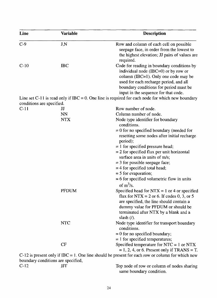
C-9 J,N Row and column of each cell on possibleseepage face, in order from the lowest to the highest elevation; JJ pairs of values are required.

C-10 IBC Code for reading in boundary conditions byindividual node (IBC=0) or by row or column (IBC=1). Only one code may be used for each recharge period, and all boundary conditions for period must be input in the sequence for that code.

Line set C-l 1 is read only if IBC = 0. One line is required for each node for which new boundary conditions are specified. C-11 JJ Row number of node.

NN Column number of node.NTX Node type identifier for boundary

conditions.= 0 for no specified boundary (needed for

resetting some nodes after initial recharge period);

= 1 for specified pressure head; = 2 for specified flux per unit horizontal

surface area in units of m/s; = 3 for possible seepage face; = 4 for specified total head; = 5 for evaporation; = 6 for specified volumetric flow in units

of m3/s.PFDUM Specified head for NTX = 1 or 4 or specified

flux for NTX = 2 or 6. If codes 0, 3, or 5 are specified, the line should contain a dummy value for PFDUM or should be terminated after NTX by a blank and a slash (/).

NTC Node type identifier for transport boundaryconditions.

= 0 for no specified boundary; = 1 for specified temperatures;

CF Specified temperature for NTC = 1 or NTX= 1, 2, 4, or 6. Present only if TRANS = T.

C-12 is present only if IBC = 1. One line should be present for each row or column for which new boundary conditions are specified,C-12 JJT Top node of row or column of nodes sharing

same boundary condition.

24

Line Variable Description

C-12 (Continued) JJB Bottom node of row or column of nodeshaving same boundary condition. Will equal JJT if a boundary row is being read.

NNL Left column in row or column of nodeshaving same boundary condition.

NNR Right column of row or column of nodeshaving same boundary condition. Will equal NNL if a boundary column is being read in.

NTX Same as line C-ll. PFDUM Same as line C-ll. NTC Same as line C-ll. CF Same as line C-ll.

C-13 Designated end of recharge period. Must be included after line C-12 datafor each recharge period. Two C-13 lines must be included after final recharge period. Line must always be entered as -999999 /.

25

APPENDIX 2Example Problem Input

1-D unsaturated 3600. 0. 0.

M SEC J 3 129 168 2400 F T T T T F T F T T F F F T F F 1 1.00 1.00.0010.0010.0210.3960.5000.5000.5000.5000.5000.5000.5000.5000.5001

0.0.0.0.0.0.0.0.0.0.0.0.0.

001001021500500500500500500500500500500

0000000000000

flow

.001

.0015

.029

.500

.500

.500

.500

.500

.500

.500

.500

.500

.500

with energy transport (Jaynes, 1990) A2 TMAX,STIM,ANG A3 ZUNIT , TUNIT , CUNX A4 NXR,NLY A5 NRECH,NUMT A6 RAD, ITSTOP, TRANS A6A--CIS,CIT,SORP A7 F11P,F7P,F8P,F9P,F6P A8 THPT , SPNT , PPNT , HPNT , VPNT A9 IFAC,FACX

0.001 0.0.0015 0.0.037 0.0.500 0.0.500 0.0.500 0.0.500 0.0.500 0.0.500 0.0.500 0.0.500 0.0.500 0.0.500 0.

001002047500500500500500500500500500500

0000000000000

3600.322 225 229 213l.e-7 _ 90 0 .00 l.Oe-10 l.Oe-72 199T26611. 4.0.0121. 8.0.0111 3

Oe-08 .0. 01 2.

Oe-06 .0.

71 3 1292 1.100.F F0 21.3600.

-

30

01

12

0.

2.

0 . 496 -118e+6 1.5

0 . 496 -118e+6 1.5

.18 .15 4 .81.8 4.18e+6

.18 .15 4 .81.8 4.18e+6

7497

360.1.2 3600.100.0.0FF F F0221128 2

0.

01

-999999-999999

180.

.04050//

.00

0.5

17.48

A11--IFAC,FACZ.001 0.001 0.001 0.001.003 0.005 0.010 0.015.061 0.091 0.131 0.187.500 0.500 0.500 0.500.500 0.500 0.500 0.500.500 0.500 0.500 0.500.500 0.500 0.500 0.500.500 0.500 0.500 0.500.500 0.500 0.500 0.500.500 0.500 0.500 0.500.500 0.500 0.500 0.500.500 0.500 0.500 0.500.500 0.500 0.500 0.500

A13--NPLTA14--PLTIMA15--NOBS

A17--NMB9A18--MB9Bl EPS,HMAX,WUS,EPS1,B3- MINIT, ITMAXB4 PHRDB5 - - -NTEX , NPROP , NPROPlB6---ITEXB7 ANIZ,HKB7A--HTB6 ITEXB7 ANIZ,HKB7A--HTB8 IROWB10--IL,IR, JBT, JRDB10--IL,IR, JBT, JRDB11--IREAD, FACTORB12 DWTX,HMINB14--BCIT, ETSIMB24--IREAD, FACTORC1---TPER,DELTC2 TMLT, DLTMX, DLTMIN,C3 DSMAX,STERRC4- PONDC5 PRNTC6 BCIT, ETSIM, SEEPCIO IBC

000000000000

.001

.020

.261

.500

.500

.500

.500

.500

.500

.500

.500

.500

EPS2

TRED

Cll JJ,NN,NTX, PFDUM,NTC,1 21.30 C11--JJ,NN,NTX,PFDUM,NTC,

C13C13

CFCF

26

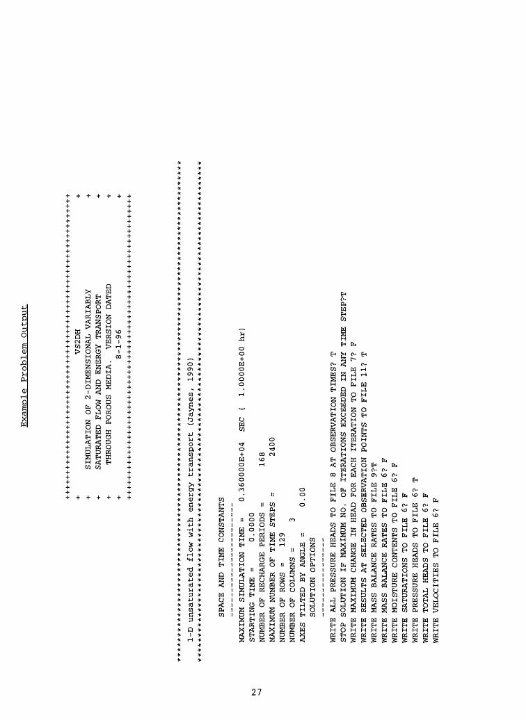
Example Problem Output

+ VS

2DH

++

SIMULATION OF 2-DIMENSIONAL VARIABLY

++

SATURATED FLOW AND ENERGY TRANSPORT

++

THROUGH POROUS MEDIA.

VERSION DATED

++

8-1-96

+

1-D un

satu

rate

d flow with

energy tr

ansp

ort

(Jaynes, 1990)

***************************************************************************************

SPACE AND TIME CONSTANTS

MAXIMUM SIMULATION TIME =

0.360000E+04

SEC

( l.OOOOE+00 hr)

STARTING TIME =

0.0000

NUMBER OF RECHARGE PERIODS =

168

MAXIMUM NUMBER OF TIME STEPS =

2400

NUMBER OF ROWS =

129

NUMBER OF COLUMNS =

3 AXES TILTED BY ANGLE =

0.00

SOLUTION OPTIONS

WRITE ALL PRESSURE HEADS TO FILE 8 AT OBSERVATION TIMES? T

STOP SOLUTION IF MAXIMUM NO. OF ITERATIONS EXCEEDED IN ANY TIME STEP?T

WRITE MAXIMUM CHANGE IN HEAD FOR EACH ITERATION TO FILE 7? F

WRITE RESULTS AT SELECTED OBSERVATION POINTS TO FILE 11? T

WRITE MASS BALANCE RATES TO FILE 9?T

WRITE MASS BALANCE RATES TO FILE 6? F

WRITE MOISTURE CONTENTS TO FILE 6? F

WRITE SATURATIONS TO FILE 6? F

WRITE PRESSURE HEADS TO FILE 6? T

WRITE TOTAL HEADS TO FILE 6? F

WRITE VELOCITIES TO FILE 6? F

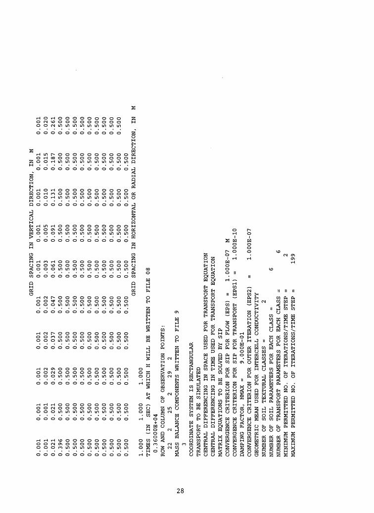
GRID SPACING IN VERTICAL DIRECTION, IN M

0.001

0.001

0.021

0.396

0.500

0.500

0.500

0.500

0.500

0.500

0.500

0.500

0.500

0. 0. 0. 0. 0. 0. 0. 0. 0. 0. 0. 0. 0.

001

001

021

500

500

500

500

500

500

500

500

500

500

0.001

0.00

20.029

0.500

0.500

0.500

0.500

0.500

0.500

0.500

0.500

0.500

0.500

0.001

0.002

0.037

0.500

0.500

0.500

0.500

0.500

0.500

0.500

0.500

0.500

0.500

0.001

0.002

0.047

0.500

0.500

0.500

0.500

0.500

0.500

0.500

0.500

0.500

0.500

0. 0. 0. 0. 0. 0. 0. 0. 0. 0. 0. 0. 0.

001

003

061

500

500

500

500

500

500

500

500

500

500

0. 0. 0. 0. 0. 0. 0. 0. 0. 0. 0. 0. 0.

001

005

091

500

500

500

500

500

500

500

500

500

500

0 0 0 0 0 0 0 0 0 0 0 0 0

.001

.010

.131

.500

.500

.500

.500

.500

.500

.500

.500

.500

.500

0 0 0 0 0 0 0 0 0 0 0 0 0

.001

.015

.187

.500

.500

.500

.500

.500

.500

.500

.500

.500

.500

0.001

0.020

0.261

0.500

0.500

0.500

0.500

0.500

0.500

0.500

0.500

0.500

GRID SPACING IN HORIZONTAL OR RADIAL DIRECTION, IN M

1.000

1.000

1.000

TIMES (IN

SEC) AT WHICH H WILL BE WRITTEN TO FILE 08

0.36000E+04

ROW AND COLUMN OF OBSERVATION POINTS:

22

2 25

2 29

2MASS BALANCE COMPONENTS WRITTEN TO FILE 9

3COORDINATE SYSTEM IS RECTANGULAR

TRANSPORT TO BE SIMULATED

CENTRAL DIFFERENCING IN SPACE USED FOR TRANSPORT EQUATION

CENTRAL DIFFERENCING IN TIME USED FOR TRANSPORT EQUATION

MATRIX EQUATIONS TO BE SOLVED BY SIP

CONVERGENCE CRITERION FOR SIP FOR FLOW (EPS)

= l.OOOE-07

MCONVERGENCE CRITERION FOR SIP FOR TRANSPORT (EPS1) =

l.OOOE-10

DAMPING FACTOR, HMAX =

9.000E-01

CONVERGENCE CRITERION FOR OUTER ITERATION (EPS2)

=

l.OOOE-07

GEOMETRIC MEAN USED FOR INTERCELL CONDUCTIVITY

NUMBER OF SOIL TEXTURAL CLASSES =

2NUMBER OF SOIL PARAMETERS FOR EACH CLASS =

6NUMBER OF TRANSPORT PARAMETERS FOR EACH CLASS =

6MINIMUM PERMITTED NO. OF ITERATIONS/TIME STEP =

2MAXIMUM PERMITTED NO. OF ITERATIONS/TIME STEP =

199

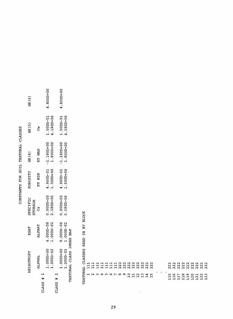
CONSTANTS FOR SOIL TEXTURAL CLASSES

ANISOTROPY

ALPHAL

CLASS #

1l.OOOD+00

l.OOOD-02

CLASS #

2l.OOOD+00

l.OOOD-02

TEXTURAL CLASS

TEXTURAL CLASSES

1 111

2 111

3 111

4 111

5 111

6 111

7 111

8 222

9 22

210

22

211

222

12

222

13

222

14

222

15

222

115

222

116

222

117

222

118

222

119

222

120

222

121

222

122

222

123

222

KSAT

SPECIFIC

STORAGE

ALPHAT

Cs

4.000D-08

O.OOOD+00

l.OOOD-02

2.180D+06

8.000D-06

O.OOOD+00

l.OOOD-02

2.180D+06

INDEX MAP

READ IN BY BLOCK

HK(6)

4.800D+00

4.800D+00

124

222

125

222

126

222

127

222

128

222

129

222

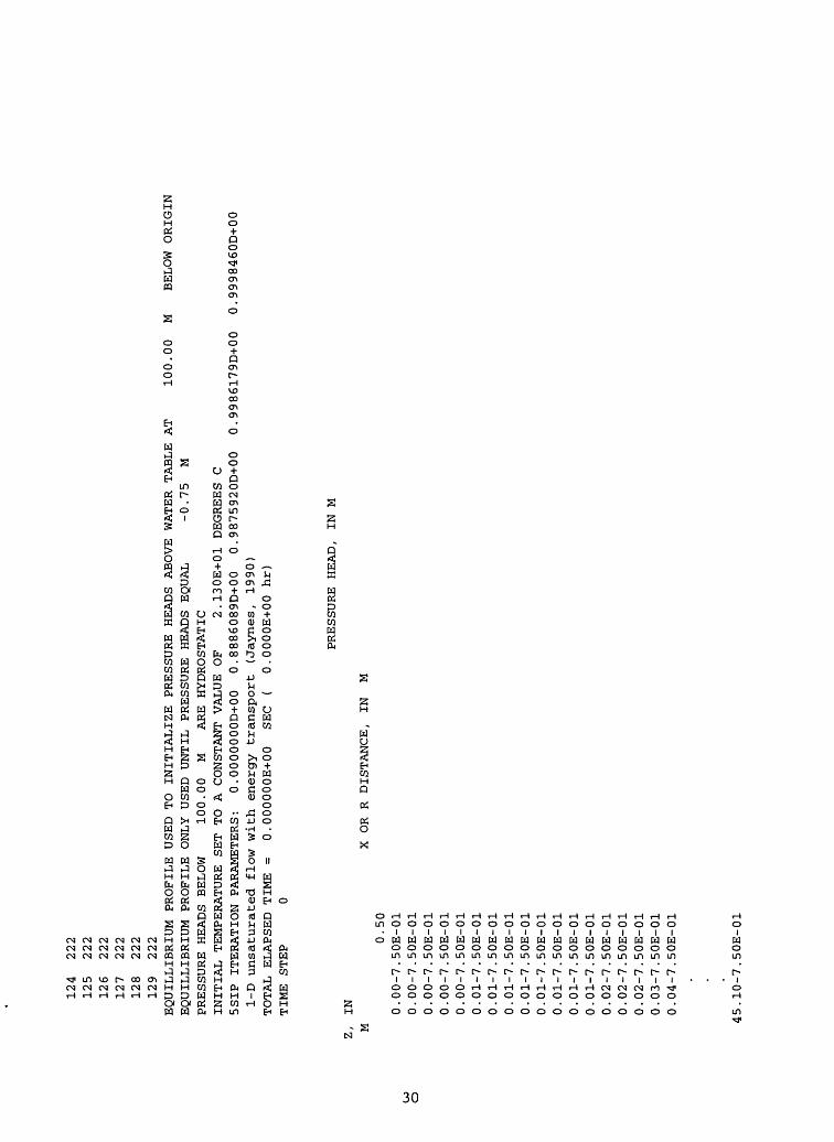
EQUILLIBRIUM PROFILE USED TO INITIALIZE PRESSURE HEADS ABOVE WATER TABLE AT

100.00

M

BELOW ORIGIN

EQUILLIBRIUM PROFILE ONLY USED UNTIL PRESSURE HEADS EQUAL

-0.75 M

PRESSURE HEADS BELOW

100.00

M

ARE HYDROSTATIC

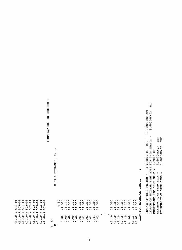
INITIAL TEMPERATURE SET TO A CONSTANT VALUE OF

2.130E+01 DEGREES C

5SIP ITERATION PARAMETERS:

0.OOOOOOOD+00

0.8886089D+00

0.9875920D+00

0.9986179D+00

0.9998460D+00

1-D unsaturated flow with energy transport (J

ayne

s, 19

90)

TOTAL ELAPSED TIME =

O.OOOOOOE+00

SEC

( O.OOOOE+00 hr

) TIME STEP

0

PRESSURE HEAD, IN M

Z, IN

M

X OR R DISTANCE, IN M

0.50

0.00-7.50E-01

O

0.00-7.50E-01

0.00-7.50E-01

0.00-7.50E-01

0.00-7.50E-01

0.01-7.50E-01

0.01-7.50E-01

0.01-7.50E-01

0.01-7.50E-01

0.01-7.50E-01

0.01-7.50E-01

0.01-7.50E-01

0.01-7.50E-01

0.02-7.50E-01

0.02-7.50E-01

0.02-7.50E-01

0.03-7.50E-01

0.04-7.50E-01

45.10-7.50E-01

45.60-7.50E-01

46.10-7.50E-01

46.60-7.50E-01

47.10-7.50E-01

47.60-7.50E-01

48.10-7.50E-01

48.60-7.50E-01

49.10-7.50E-01

49.60-7

Z, IN

M

0 0 0 0 0 0 0 0 0 0 0

46 46 47 47 48 48 49 49

.00

.00

.00

.00

.00

.01

.01

.01

.01

.01

.01

.10

.60

.10

.60

.10

.60

.10

.60

.50E-01

0.50

21.300

21.300

21.300

21.300

21.300

21.300

21.300

21.300

21.300

21.300

21.300

21.300

21.300

21.300

21.300

21.300

21.300

21.300

21.300

TEMPERATURE, IN DEGREES C

X OR R DISTANCE, IN M

DATA FOR RECHARGE PERIOD

1

LENGTH OF THIS PERIOD =

3.60000E+03

SEC

( l.OOOOE+00 hr)

LENGTH OF INITIAL TIME STEP FOR THIS PERIOD =

3.60000E+02

SEC

MULTIPLIER FOR TIME STEP =

1.200E+00

MAXIMUM TIME STEP SIZE =

3.60000E+03

SEC

MINIMUM TIME STEP SIZE =

1.80000E+02

SEC

U)

NJ

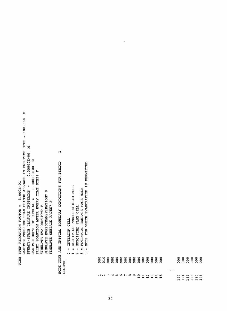
TIME STEP REDUCTION FACTOR =

5.000E-01

MAXIMUM PRESSURE HEAD CHANGE ALLOWED IN ONE TIME STEP =

100.000

MSTEADY-STATE CLOSURE CRITERION =

O.OOOOOE+00

MMAXIMUM DEPTH OF PONDING =

O.OOOOOE+00

MPRINT SOLUTION AFTER EVERY TIME STEP? F

SIMULATE EVAPORATION? F

SIMULATE EVAPOTRANSPIRATION? F

SIMULATE SEEPAGE FACES? F

NODE TYPE AND INITIAL BOUNDARY CONDITIONS FOR PERIOD

1 LEGEND:

0 =

INTERIOR CELL

1 = SPECIFIED PRESSURE HEAD CELL

2 = SPECIFIED FLUX CELL

3 = POTENTIAL SEEPAGE FACE NODE

5 = NODE FOR WHICH EVAPORATION IS PERMITTED

1 2 3 4 5 6 7 8 910 11 12 13 14 15

000

010

000

000

000

000

000

000

000

000

000

000

000

000

000

120

000

121

000

122

000

123

000

124

000

125

000

126

127

128

129

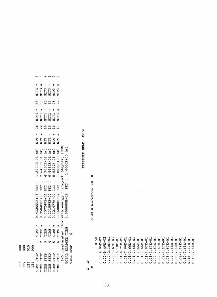
TIME

TIME

TIME

TIME

TIME

TIME

STEP

STEP

STEP

STEP

STEP

STEP

000

000

010

000

1 2 3 4 5 6

TIME

TIME

TIME

TIME

TIME

TIME

1-D unsaturated flow

TOTAL ELAPSED TIME =

TIME STEP

6

0.432000E+03 SEC

( 1.

0.950400E+03 SEC

( 2.

0.157248E+04 SEC

( 4.

0.231898E+04 SEC

( 6.

0.321477E+04 SEC

( 8.

0.360000E+04 SEC

( 1.

with energy transport

3.600000E+03

SEC

( 1

2000E-01 hr)

6400E-01 hr)

3680E-01 hr)

4416E-01 hr)

9299E-01 hr)

OOOOE+00 hr)

(Jaynes, 1990)

.OOOOE+00 hr)

NIT

NIT

NIT

NIT

NIT

NIT

= = = = = =

26 22 16 15 16 13

NITl

NITl

NITl

NITl

NITl

NITl

= = = = = =

35 35 25 25 25 22

NIT3

NIT3

NIT3

NIT3

NIT3

NIT3

= = = = = =

3 3 2 2 2 2

PRESSURE HE

AD,

IN M

Z, IN

M

0. 0. 0. 0. 0. 0. 0. 0. 0. 0. 0. 0. 0. 0. 0. 0. 0. 0. 0. 0. 0. 0. 0.

00 4

00-9

00-2

00-3

00-5

01-6

01-7

01-7

01-7

01-7

01-7

01-7

01-7

02-7

02-7

02-7

03-7

04-7

06-7

08-7

10-7

13-7

16-7

0.50

.05E

-02

.46E

-02

.30E-01

.67E-01

.10E-01

.71E-01

.66E-01

.66E-01

.66E-01

.66E-01

.66E-01

.67E-01

.67E-01

.67E-01

.67E-01

.67E-01

.67E-01

.68E-01

.68E-01

. 68E-01

. 68E-01

. 67E-01

.66E-01

X OR R DISTANCE, IN

M

0.20-7.65E-01

0.25-7.63E-01

0.33-7.61E-01

0.44-7.59E-01

0.60-7.56E-01

0.82-7.53E-01

1.15-7.51E-01

1.60-7.50E-01

2.10-7.50E-01

2.60-7.50E-01

45.10-7.50E-01

45.60-7.50E-01

46.10-7.50E-01

46.60-7.50E-01

47.10-7.50E-01

47.60-7.49E-01

48.10-7.42E-01

48.60-6.68E-01

49.10-3.61E-01

49.60 O.OOE+00

TEMPERATURE, IN DEGREES C

X OR R DISTANCE, IN M

Z, IN

M

0. 0. 0. 0. 0. 0. 0. 0. 0. 0. 0. 0. 0. 0. 0.

00 00 00 00 00 01 01 01 01 01 01 01 01 02 02

17 17 17 17 17 17 17 17 17 17 17 17 17 17 18

0.50

.480

.480

.492

.513

.540

.572

.606

.642

.679

.717

.755

.801

.856

.918

.004

OJ

0.02

0.03

0.04

0.06

0.08

0.10

0.13

0.16

0.20

0.25

0.33

0.44

0.60

0.82

45.10

45.60

46.10

46.60

47.10

47.60

48.10

48.60

49.10

49.60

18.135

18.377

18.806

19.411

20.024

20.506

20.906

21.162

21.268

21.296

21.300

21.300

21.300

21.300

21.300

21.300

21.300

21.300

21.300

21.300

21.300

21.300

21.300

21.300

PUMPING PERIOD NUMBER

1

TOTAL ELAPSED SIMULATION TIME =

3.600000E+03

SEC

+++++++++++++++++++++++++++++++++++++++++++++++++++++++++++++++++++++++++

VOLUMETRIC FLOW BALANCE

FLUX INTO DOMAIN ACROSS SPECIFIED PRESSURE HEAD BOUNDARIES

FLUX OUT OF DOMAIN ACROSS SPECIFIED PRESSURE HEAD BOUNDARIES --

FLUX INTO DOMAIN ACROSS SPECIFIED FLUX BOUNDARIES --

FLUX OUT OF DOMAIN ACROSS SPECIFIED FLUX BOUNDARIES --

TOTAL FLUX INTO DOMAIN --

TOTAL FLUX OUT OF DOMAIN --

EVAPORATION

TRANSPIRATION

TOTAL EVAPOTRANSPIRATION

CHANGE IN FLUID STORED IN DOMAIN --

FLUID VOLUME BALANCE --

ENERGY MASS BALANCE

FLUX INTO DOMAIN ACROSS SPECIFIED PRESSURE HEAD BOUNDARIES

FLUX OUT OF DOMAIN ACROSS SPECIFIED PRESSURE HEAD BOUNDARIES --

FLUX INTO DOMAIN ACROSS SPECIFIED FLUX BOUNDARIES --

FLUX OUT OF DOMAIN ACROSS SPECIFIED FLUX BOUNDARIES --

DIFFUSIVE/DISPERSIVE FLUX INTO DOMAIN

DIFFUSIVE/DISPERSIVE FLUX OUT OF DOMAIN

TOTAL FLUX INTO DOMAIN --

TOTAL FLUX OUT OF DOMAIN --

TOTAL EVAPOTRANSPIRATION

FIRST ORDER DECAY --

ADSORPTION/ ION EXCHANGE

CHANGE IN ENERGY STORED IN DOMAIN --

ENERGY MASS BALANCE --

+++++++++++++++++++++++++++++++++++++++++++++++++++++++++++++++++++

END OF SIMULATION

2-2

0 0 2-2

0 0 0 3-1 1-2 0 0 9-4 1-7 0 0 0 8

-1

++++++

( l.OOOOE+00 hr)

+++++++++++++++++++++++++++++4

TOTAL THIS

TOTAL

M

**3

.13977E-02

.88736E-03

.OOOOOE+00

.OOOOOE+00

.13977E-02

.88736E-03

.OOOOOE+00

.OOOOOE+00

.OOOOOE+00

.26367E-02

.41264E-02

J.60997E+06

.57073E+05

.OOOOOE+00

.OOOOOE+00

.49780E-02

.56388E+05

.60997E+06

.13461E+05

.OOOOOE+00

.OOOOOE+00

.OOOOOE+00

.97832E+05

.32277E+03

+++++++++++++

TIME STEP

1-8 0 0 1

-8 0 0 0 1-1 1-7 0 0 2

-2

1-9 0 0 0 4

-1

+++++

M

**3

.96995E-03

.73949E-04

.OOOOOE+00

.OOOOOE+00

.96995E-03

.73949E-04

.OOOOOE+00

.OOOOOE+00

.OOOOOE+00

.09600E-03

.59325E-10

J

.43937E+05

.78112E+04

.OOOOOE+00

.OOOOOE+00

.32151E-02

.12911E+04

.43937E+05

.91022E+04

.OOOOOE+00

.OOOOOE+00

.OOOOOE+00

.49999E+04

.65295E+02

+++++++++++->

-++++++++++++++

RATE THIS

TIME STEP

M

5.-2

. 0. 0. 5.-2

. 0. 0. 0. 2.-4

. J 3.-2

. 0. 0. 6.-5

. 3.-2

. 0. 0. 0. 1.-4

.

+ + + + 4

**3/ SEC

11370E-06

26865E-06

OOOOOE+00

OOOOOE+00

11370E-06

26865E-06

OOOOOE+00

OOOOOE+00

OOOOOE+00

84505E-06

13585E-13

/ SEC

73640E+02

01987E+02

OOOOOE+00

OOOOOE+00

02632E-05

52686E+01

73640E+02

57256E+02

OOOOOE+00

OOOOOE+00

OOOOOE+00

16813E+02

29082E-01

-+++++++++

TOTAL NUMBER OF ITERATIONS FOR FLOW EQUATION =

191

TOTAL NUMBER OF ITERATIONS FOR TRANSPORT EQUATION =

TOTAL NUMBER OF ITERATIONS FOR OUTER LOOP =

14

294