documentos de trabajo - bde.es · debt sustainability and procyclical fiscal policies in latin...

DEBT SUSTAINABILITYAND PROCYCLICAL FISCALPOLICIES IN LATIN AMERICA

Documentos de Trabajo N.º 0611

Enrique Alberolaand José Manuel Montero

2006

DEBT SUSTAINABILITY AND PROCYCLICAL FISCAL POLICIES IN LATIN

AMERICA

DEBT SUSTAINABILITY AND PROCYCLICAL FISCAL POLICIES

IN LATIN AMERICA

Enrique Alberola and José Manuel Montero (*)

BANCO DE ESPAÑA

(*) Luis Molina crucially helped in the construction of the data base. Comments by Igor Paunovic, Iikka Korhonen andparticipants at the seminars in CEMLA Lima, LACEA Paris, REDIMA Santiago and the Third Workshop on EmergingMarkets in Madrid are gratefully acknowledged. The opinions expressed in this documents are solely responsibility of the authors and do not represent the views of the Banco de España. Contact authors: [email protected], [email protected].

Documentos de Trabajo. N.º 0611

2006

The Working Paper Series seeks to disseminate original research in economics and finance. All papers have been anonymously refereed. By publishing these papers, the Banco de España aims to contribute to economic analysis and, in particular, to knowledge of the Spanish economy and its international environment. The opinions and analyses in the Working Paper Series are the responsibility of the authors and, therefore, do not necessarily coincide with those of the Banco de España or the Eurosystem. The Banco de España disseminates its main reports and most of its publications via the INTERNET at the following website: http://www.bde.es. Reproduction for educational and non-commercial purposes is permitted provided that the source is acknowledged. © BANCO DE ESPAÑA, Madrid, 2006 ISSN: 0213-2710 (print) ISSN: 1579-8666 (on line) Depósito legal: M.22877-2006 Imprenta del Banco de España

Abstract

The computation of structural primary balances for the nine main Latin American countries

and their comparison of their changes with their cyclical position during the period

1981-2004 confirms that fiscal policy is procyclical in the region. From this evidence, the

paper shows strong evidence that the fiscal behaviour is closely linked to the financial

vulnerability position of the economies and in particular to the perception on the

sustainability of debt. The current threshold balance, defined as the primary balance which

would render the debt stable under the existing economic and financial conditions, is used

as our gauge for measuring debt sustainability at each point in time. The empirical analysis

reveals that the fiscal stance tightens when the debt sustainability perceptions worsen, and

that this effect is stronger the less sustainable debt is perceived. The results are robust to

different specifications and estimation methods.

Keywords: procyclical fiscal policy, debt sustainability.

JEL Classification: H6, E6, F3.

BANCO DE ESPAÑA 9 DOCUMENTO DE TRABAJO N.º 0611

1 Introduction

Fiscal policy is expected to play an important stabilizing role over the business cycle. When

the economy is accelerating, the fiscal authorities should be able to moderate activity by

restraining the fiscal stance and, vice versa, in downturns fiscal policy can help stimulating

the economy. Therefore, under these circumstances, fiscal policy is expected to behave

countercyclically. However, the empirical evidence has repeatedly shown that fiscal policy has

been procyclical in many countries, in particular in Latin America1. This is a rather unfortunate

feature of the region, since it introduces an additional source of volatility to the economy,

so that when the economy expands, it reinforces the expansion; when it contracts, it deepens

the slowdown. Also, according to Serven (1998), among others, the increase in volatility

reduces investment and growth.

The neoclassical theory of fiscal policy [Barro (1979)] conveys tax smoothing as a

way to accommodate transitory shocks to activity, as long as the intertemporal budget

constraint is fulfilled. In those circumstances public debt fluctuations act as a buffer stock for

shocks to activity and they enable fiscal policy to play its countercyclical role. The question is

what happens when (negative) economic shocks strongly impinge on the level of debt, too,

arising concerns about the fulfilment of the intertemporal budget constraint or, in other words,

on the sustainability of debt. In those cases the mechanism is short-circuited and this can

jeopardise the stabilizing role of fiscal policy.

This seems to be the case in Latin America. Gavin and Perotti (1997) have observed

that there creditworthiness and sustainability concerns are central to determine fiscal stances.

The dependence of Latin American finances on external sources of credit and the periodic

recurrence of sudden stops, that is, the abrupt loss of access to external credit and the

volatility of financial indicators –reflected on volatility in the debt stock and service– are behind

this situation. Furthermore, periods of difficult access to international capital markets tend to

induce restrictive macroeconomic policies, but they also translate into large current account

reversals, which are catalysed, among other channels, through economic downturns. The

slowdown in economic activity aggravates the fiscal solvency which, in turn, calls for an

additional tightening. Hence, the capital flow cycle and the macroeconomic policy cycle tend

to reinforce each other, or, as Kaminsky, Reinhart and Vegh (2004) have labelled it, in these

economies, when it rains, it pours.

As an additional argument, Riascos and Vegh (2003) argue that the incompleteness

of financial markets in emerging economies could explain procyclical fiscal policy as the

outcome of a Ramsey problem without having to impose additional frictions.

Finally, a complementary rationale to explain fiscal procyclicality is rooted in political

economy distorsions and is related to what Lane and Tornell (1999) have labelled voracity

effects2. According to this view, the ability to run large budget surpluses in good times is

severely hampered by political pressures which, though always present, get exacerbated

in times of plenty. As a result, fiscal resources are wasted in favour of any rent-seeking group

1. See, among others, Gavin et al. (1996), Gavin and Perotti (1997), Alberola and Molina (2003), Kaminsky, Reinhart and

Vegh (2004) Talvi and Vegh (2005) or Manasse (2006). 2. See also Alesina and Tabelllini (2005).


rather than saved for bad times3. Lane (2003) provides empirical support for political economy

factors in determining the fiscal policy stance in OECD countries. This notwithstanding, he

recognizes that government debt constraints can seriously limit the room for manouver for

fiscal policy in emerging markets.

It is remarkable that, notwithstanding the conventional wisdom that fiscal policy is

procycllical in Latin America, the empirical approaches in order to test the issue and explain

the reasons in a rigorous way have been scant. The main reason has probably been the

difficulty to derive adequate gauges for the fiscal stance in Latin America, due to lack or

inadequacy of data and to the extreme volatility of macroeconomic and financial variables in

the region. These factors have hindered the computation of structural fiscal balances, which

is the most common indicator to assess the fiscal stance in OECD countries. That is why

most papers have studied this issue analyzing the cyclical correlations between government

spending, tax rates, the overall fiscal balance and the primary fiscal balance and the GDP

cycle4.

In this paper, we aim at overcoming these problems in order to explore in a

systematic way whether and how the perception of creditworthiness and debt sustainability

is key to explain the procyclicality of fiscal policy. We build on previous evidence by

Alberola and Molina (2003), who show that in emerging markets fiscal balances are

determined by the financing costs and that they are closely related to the cycle. Our approach

is related to the empirical literature on fiscal rules and fiscal policy sustainability [see, inter

alia, Bohn (1998)]. The focus of this literature lies on whether governments react to debt

accumulation by increasing primary balances or not, such that their fiscal behaviour is

consistent with the intertemporal budget constraint. However, in this alternativa approach

the focus is on the mean reverting properties of debt, that is on long-run, thus dismissing,

on the one hand, the cyclical components and on the other hand, the temporary swings in

debt sustainability perception which are at the core of our hypothesis.

Our strategy consists of two steps. First, we check the procyclicality of fiscal policy.

Second, we search for an explanation to this behaviour, focusing on the perceived

creditworthiness of the country, which, simultaneously influences and is influenced by the

access to external credit.

To attain the first goal, we compute the structural primary balance for nine countries

of the region for the period 1981-2004, taking advantage of recent improvements in filtering

techniques to derive the output gap. The changes in the structural primary balance define

the fiscal stance which is compared to the cyclical position of the economy: an increase in the

structural balance at a time of economic upturn would signal a countercyclical and, thus,

stabilising role for fiscal policy.

Secondly, the perceived creditworthiness of a country is closely related to its

indebtedness position. While the level of debt to GDP is not too large, specially when

compared to other developed countries like some EU states or Japan, Latin America suffers

3. The theory behind this argument is that interest groups view fiscal resources as a common pool and they compete for

a share in that pool. Each group will be unwilling to reduce its claim on an increase in fiscal resources, knowing that the

benefits of this moderation would accrue to other interest groups. Therefore, deviations from a countercyclical policy

may be an indirect way of fending off spending pressure through, for instance, tax cuts when the economy is in

expansion. But it will not be optimal to resist all spending pressures, so government spending is also expected to

increase.

4. For a thorough discussion of the problems posed by this methodology see Kaminsky, Reinhart and Vegh (2004).


from debt intolerance, as Reinhart, Rogoff and Savastano (2002) have labelled it. This

intolerance can be explained by the previous history of debt defaults, economic instability

and weak institutions, which determine not only a higher financing cost, but also a debt

structure that is biased towards foreign currency and short maturities. These features

combine with the tendency to suffer dramatic swings in the financing conditions, which

impinge on the perception of creditworthiness and may even cut off their access to the

international financial markets. Under these circumstances, the critical debt thresholds are

much lower than in the OECD countries and the financing conditions display a higher volatility.

Hence, the use in the second part of the paper of an indicator of debt sustainability

to assess fiscal creditworthiness. Furthermore, debt dynamics are very sensitive to financing

conditions. This means both that the assessment of creditworthiness can be quite volatile and

that it can be self-feeding as long as the perception of vulnerability affects the evolution of

financial variables. As a matter of fact, we depart from previous contributions by stressing

the role played by current financing conditions in determining public debt sustainability. More

precisely, we define the current threshold balance as the primary balance which renders

public debt stable at each point in time. Primary balances above such threshold would imply

that the debt is sustainable. This indicator will be used to uncover the relation between the

fiscal stance and public debt sustainability.

We find a strong empirical backing for our hypothesis. First, the panel data analysis

shows a strong and significant negative correlation between the changes in the structural

primary balance and the output gap, so that they confirm that fiscal policy is procyclical in

Latin America. After having stated this, we move on to show how debt sustainability issues

affect the fiscal behaviour. The empirical evidence shows that a deterioration of the current

threshold balance induces a fiscal tightening and that this tightening tends to be stronger the

worse the initial debt sustainability position is5. These results can be taken as strong evidence

that debt sustainability concerns play a determinant role in explaining the fiscal behaviour in

Latin America and the procyclical bias of fiscal policy. In fact, it is shown that for most of the

specifications public debt sustainability concerns seem to account, from a statistical point of

view, for the whole procyclicality of fiscal policy in Latin America.

The rest of the paper is organized as follows. The next section describes the method

employed to compute structural primary balances and studies whether fiscal policy is

procyclical or not. Section 3 explains how an indicator of fiscal sustainability is constructed

and then, it analyzes whether the fiscal stance is related to the sustainability of public debt.

Section 4 contains some concluding remarks.

5. Note that this approach is somehow related to the empirical literature on fiscal rules and fiscal policy sustainability

[see, inter alia, Bohn (1998)]. The focus of this literature lies on whether governments react to debt accumulation

by increasing primary balances or not, such that their fiscal behaviour is consistent with the intertemporal budget

constraint. The idea is that a positive response of the primary balance to public debt ensures that any upward movement

in the debt to GDP ratio due to negative shocks (e. g., low growth, wars, higher interest rates) would be eventually

reversed through primary surpluses.


2 The procyclicality of fiscal policy

The specification of structural or cyclically-adjusted balances has centered a great deal of

effort to come up with a universally accepted methodology to separate the budget balance

into its structural and cyclical components. All the available methods involve two main

steps. First, the cyclical fluctuations (output gaps) are derived by subtracting the potential

or trend output from actual output and expressing the difference as a percentage of the

former. Second, the cyclical component of the budgetary balance is estimated through

the application of fiscal elasticities to GDP and, for some cases, commodity prices.

Finally, this cyclical component is deducted from the actual budget balance to derive

the structural (cyclically-adjusted) component. This is the approach used by most of the

international organizations and national authorities. The main difference among methodologies

involves the calculation of the output gap, which is estimated either via a smoothing technique

(Hodrick-Prescott) or through a production function [Giorno et al. (1995)].

Structural balances is a widely used tool to assess the fiscal stance in industrialized

countries, where the availability of long term statistics and the relative stability of the economic

environment has allowed to develop increasingly improved techniques to filter out the cyclical

balances. In fact, in the last years a preference has been observed towards the second

method (which was already used by OECD and IMF), after the shift of the EC towards it.

Estimates of the cycle based on this method require the availability of reliable data on the use

of labour and capital stocks.

In Latin America, the computation of structural balances has traditionally been

hindered by the lack of long series of data, the extreme volatility of the macroeconomic

variables and the noise in the fiscal data derived from dramatic structural changes and/or

composition of revenues and expenditure. Furthermore the volatility of revenues is closely

associated to the evolution of commodity prices and exports which, in several countries, are

an important source of fiscal financing. Given these obstacles, and in spite of the recent

efforts made in some countries, like Chile, the estimates of structural balances for the

countries in the region are scant and a joint estimation of these balances for the whole region

is, to our knowledge, non-existent6. Here, as a starting point to our empirical analysis, we aim

at filling this gap by estimating the primary structural balances for the nine main countries of

Latin America.

The methodology we will use to derive the trend output is smoothing through the

Hodrick-Prescott (1997) filter. Since it is being abandoned in OECD countries some

motivation for this option is in order. First, lack of data availability and homogeneity. It is well

known that labour statistics in Latin America are unreliable due to the importance of

the informal economy and that capital stocks are difficult to measure in general, and more

prominently in these countries; second, given the recurrence of economic crises, the concept

of potential output that underlies the use of full capacity of production factors loses

some clarity. In particular, if we think of the disruptions that economic crises provoke in

these economies, the cyclical position is clearly not the only element which drives a wedge

between potential and actual output. Finally, the recent refinement of filtering techniques

6. A notable exception is “Sostenibilidad fiscal en la región andina. Políticas e instituciones”, Corporación Andina de

Fomento (2004).


allows for a more precise estimation of the cycle, also in the cases of variables with large

variability, like in the Latin American case.

2.1 Estimation of the trend output and the primary structural balances

The trend output is calculated by applying the Hodrick-Prescott filter to the real GDP series.

Let Y denote actual real GDP and Y* real trend GDP. Then, the estimate of the output gap

(GAP) is obtained taking the quotient of the difference between GDP and trend output, that is,

1Y YGAP

Y

*

*( )

−=

In practice, we proceed along the lines set forth by Kaiser and Maravall (1999) to

improve on the performance of the Hodrick-Prescott filter. Given the high volatility of Latin

American output, we pre-adjusted the series by identifying outliers and then extracting them

from the original series. These outliers were assumed to be transitory and were, thus,

they end up assigned to the cyclical component of output. Also, to overcome accuracy

problems in both ends of the series, we added forecasts and backcasts for further periods7.

At this stage, we used actual data for the beginning of the series and forecasts from

Consensus Forecasts for the end of the sample8, instead of the model-based method

suggested by Kaiser and Maravall (1999).

Calculating cyclically-adjusted balances once the output gap measure has been

estimated involves to single out the budgetary items which are assumed to display a cyclical

pattern. In developed countries, such items usually involve different types of revenues and

some cycle-sensitive expenditures, such as unemployment benefits. However, for Latin

America, the lack of generalized unemployment subsidies and of appropriate data on this

kind of subsidies advises for a simplified scheme, where only revenues (T), taken as a whole,

are considered as cyclically sensitive. In order to filter out the cyclical part of revenues, the

elasticity of T to activity is computed from the following regression.

t t tT Ylog logα β ε= + + (2)

so that the cyclically adjusted revenues TS are estimated as9

S tt t

t

YT T

Y

* β⎛ ⎞

= ⎜ ⎟⎜ ⎟⎝ ⎠

(3)

Moreover, for an important number of Latin American countries, the revenues are

heavily influenced by commodity-related taxes or excises, which also have a bearing with

the level of activity and whose prices tend to be rather volatile, affecting the cyclical profile of

public revenues. Therefore, it is customary to address the estimation of structural primary

balances in these countries taking into account the evolution of commodities revenues. In our

sample, Mexico, Venezuela, Ecuador, Colombia –all of them oil exporters– and Chile (copper),

7. Part of the computations were carried out with the Tramo/Seats program developed by Gómez and Maravall (1996).

8. Where there were no forecasts available we employed estimates from the IMF’s Article IV reviews (Ecuador and

Uruguay).

9. The fact that the elasticity is computed on overall revenues tends to exact too much cyclicality from the revenues. This

is why it is also convenient to impose, as a robustness check, a unitary elasticity in the analysis as we will do in the next

section.


where the share fiscal revenues from commodities is substantial, the computation of

structural revenues and balance is accordingly modified:

S t tt t comm

t t

Y pT T

Y p

* *β φ⎛ ⎞ ⎛ ⎞

= ⎜ ⎟ ⎜ ⎟⎜ ⎟ ⎜ ⎟⎝ ⎠ ⎝ ⎠

(4)

where pcomm and p* are, respectively, the real prices of commodities and the notional real

equilibrium price of the commodity, and the elasticities are estimated through the following

regression:

commt t t tT Y plog log logα β φ ε= + + + (5)

The trend real commodity price (p*) is calculated by applying the Hodrick-Prescott

filter to the real price series. This method provides a desired degree of homogeneity, but at a

cost in terms of precision. The structural balance is computed by just substracting from

the cyclically-adjusted revenues the overall public expenditures (Gt). However, in order to

define more properly the fiscal stance it is pertinent, even more in Latin America, to deduce

from the expenditures the interest payments on public debt (IPt), since this is a volatile

source of expenditure which is clearly out of the discretion of the authorities. In this way,

we obtain the primary structural balance (SPBt), according to the following expression, where

it is important to note that all variables are expressed in terms of GDP,

St t t tSPB T G IP( )= − − (6)

The fiscal stance will be given by the changes in the structural primary balance

(∆SPBt). An increase (decrease) in the structural primary balance signals a contractionary

(expansionary) fiscal stance.

2.2 Fiscal stance and the cycle

Our sample covers nine Latin American countries for the period 1981 to 200410. The output

gap has been computed making use of two different λ in the Hodrick-Prescott filter: λ=6.7,

as recommended by Maravall and del Rio (2001), and λ=100, which is the usual figure and

that delivers wider cycles. The fiscal stance has required the computation of the revenue

elasticities with respect to GDP for each country and also for commodities revenues for the

aforementioned countries (see table 111). Note that the elasticities are clustered around values

higher than 1.5 for most countries, and are strongly significant for all countries but

Venezuela12.

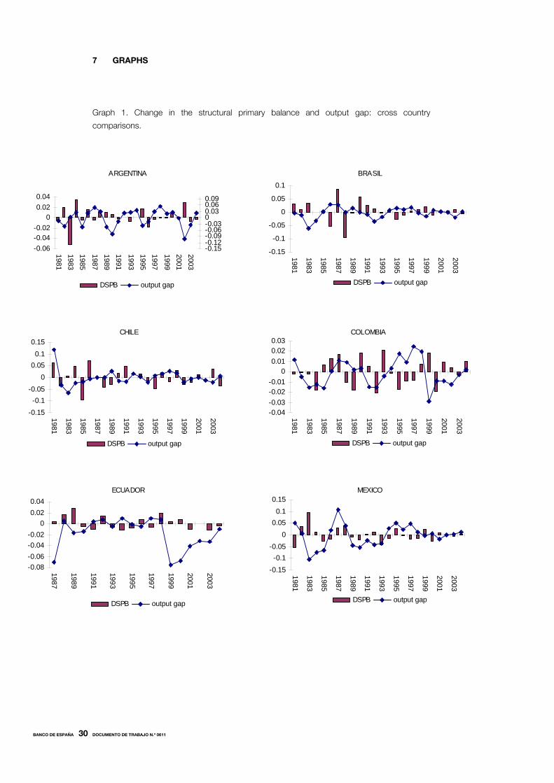
The figures in graph 1 present the output gap and the changes in the structural

balance –our gauge for the fiscal stance– of each country for λ=6.7. In the figures it can be

10. These countries are Argentina, Brazil, Chile, Colombia, Ecuador, Mexico, Peru, Uruguay and Venezuela. Our basic

sources for the fiscal variables are the IMF Government Finance Statistics and International Financial Statistics (IFS),

which have been complemented, when necessary, with national statistics. Due to data limitations fiscal variables have

been computed for the central government. GDP data come from the IFS.

11. The elasticities have been estimated by Dynamic OLS (see Stock and Watson, 1993). All the series have been

pre-adjusted with TRAMO/SEATS in order to remove outliers that might bias the estimation.

12. The case of Chile deserves particular attention. Estimates for equation (5) yielded a negative elasticity for the real

copper price, which is puzzling. Therefore, we decided to employ the GDP elasticities obtained by Marcel et al. (2001)

and a unit elasticity for the real copper price, which would be approximately equivalent to the elasticity implied by

their method. Results are not modified for copper-price elasticities around unity. In the case of the GDP elasticity, we

present the results for the lower range of their estimates (which is between 0.7 and 1.25), though the results are not

sensitive to this choice.


seen in many cases that the fiscal stance is contractionary –SPB increases– when the output

gap is negative, suggesting that the fiscal policy has been procyclical.

A proper statistical analysis of this hint appears in table 2A, where the correlation

between ∆SPBt and the output gap is negative for both λs, except in Chile and, for λ=6.7,

Ecuador. By regressing both variables, it can be observed analogously that the slope

coefficient is significantly negative –with 90% probability– in one third of the cases, and

inequivocally so in Peru and Uruguay. In the second part of the table, which uses the value

100 for λ, Argentina and Brazil are also significant. Therefore, Chile seems to be the only

country where the fiscal stance has been somehow countercyclical (a positive, though

non-significant, relationship between the output gap and the changes in SPB). For the sake of

completeness, table 2B performs the same computations but, instead of using the estimated

elasticities, these are set to one, as it is done sometimes in order to estimate the fiscal

impulse by the IMF13.

A preliminary aggregate picture for the region can be obtained by looking at

the scatter plot in graph 2. The de-meaned output gaps and changes in structural balances

are plotted against each other. The evident negative slope of the regression line confirms, at a

glance, the apparent procyclicality of fiscal policy in Latin America. For the sake of

comparison, we have also plotted the same relationship for the US14, where it is apparent that

a positive correlation exists in this case –which as it turns out is statistically significant–

denoting the expected countercyclicality of fiscal policy. It is important to note, however,

that the same analysis carried out for all OECD countries shows that in some of them fiscal

policy –according to this criterion– has been procyclical, even significantly, at least for some

parts of the period considered. This implies that the criterion is rather strict and that

the procyclicality of fiscal policies is not an exclusive feature of Latin American economies,

although here it has been more intense and protracted.

The econometric counterpart of this scatter plot is the panel data analysis which

appears in table 3 for the two λs15 considered. A panel regression of the fiscal stance on the

output gap, with both fixed and random effects, is presented. The estimated coefficient is

always negative and strongly significant, which yields a very strong and robust evidence of

the procyclicality of the fiscal stance in Latin America. The two final columns of the table

divide the sample into two periods, comparing the 80s with the 90s. It turns out that the

negative sign is not significant for the first part of the sample, although the point estimates

are quite similar. A possible reason for the weaker result in the eighties is the relevance of

monetary financing of the deficit, which may introduce some noise in the data, since inflation

enabled fiscal authorities to mask the actual deficit figures16.

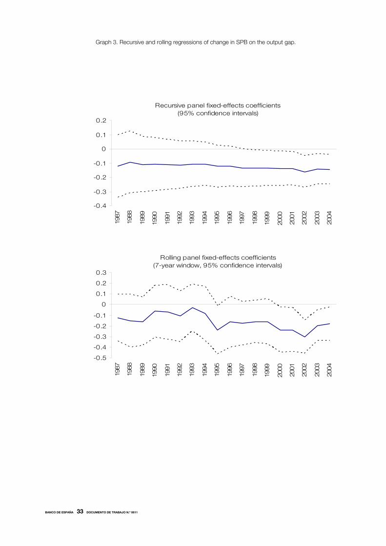
In graph 3 the notion of time stability of the parameters is further explored. The

upper chart displays the slope parameter of the previous regression in a recursive estimation,

starting with the period 1981-1987 and adding one observation at a time. The parameter is

13. The fiscal impulse also implies computing the structural public expenditures as a function of potential output, with a

unit elasticity which is, after all, very similar to just taking expenditure as given. Another reason to look at this alternative

measure is that the filtering out of overall public revenues with estimated elasticities, like in this case, tends to extract,

by construction, all the cyclicality from the revenues, not only that associated to the automatic stabilizers.

14. Both the output gap and the structural primary balance come from the OECD statistics database.

15. The results are very similar when using a unit elasticity for public revenues.

16. These results may also be driven by the presence of Chile, which is the only country with some evidence of

countercyclicality of fiscal policy. In fact, when this country is excluded from the sample, the negative sign recovers

its statistical significance for the decade of the 80s. For a more detailed analysis of the impact of inflation on public

finances. see Alberola and Molina (2003).


very stable: it moves in a very narrow range between -0.10 and -0.15, and it is significant after

the year 1997 is included. The lower chart is, alternatively, a rolling regression, starting as

before in the seven-year window 1981-1987 but deleting and adding one observation at a

time to keep unchanged the size of the window. Here, as expected, it is observed a higher

variability but again it is relatively stable. Furthermore, in this chart it can be observed that

through time, and mainly in the second half of the nineties, the fiscal policy tended to become

more procyclical17. Only the recent recovery period seems to have bucked that trend.

17. These results are again reinforced if we remove Chile from the analysis.


3 Debt sustainability and the fiscal stance

The results so far have robustly confirmed that, far from playing its expected stabilizing role,

fiscal policy has been procyclical in Latin America: economic expansions have tended to

be accompanied by expansionary fiscal policies, while the downturns of the cycle were

worsened by a contractionary fiscal stance. The rest of the paper is devoted to explaining this

puzzling result. Our main suspect is the influence that the concerns on the sustainability

of public debt have on the fiscal policy stance through the cycle.

Obviously, the level of debt is a central element in this assessment and a

fundamental constraint for fiscal policy, but it will only be expected to be effectively

binding throughout the cycle when two circumstances concur: i) debt is high enough to

influence fiscal policy in the short run, and ii) its financing conditions, including its cost, are

closely related to the cycle. As suggested in the introduction, both conditions may hold

for many Latin American countries.

3.1 An indicator of fiscal sustainability. The current threshold balance

This section is thus focused on developing a feasible indicator to explore the links

between the fiscal stance and the debt sustainability concerns. Our indicator is adapted from

a simplified, static version of the debt sustainability analysis, used among others by

Blanchard (1990)18. According to the conventional definition, debt will be sustainable at

any point of time when the value of current debt is lower than the net present value of

future primary balances, that is, the fiscal balance once the interest payments on debt are

deducted. This definition, simple as it is, faces the problem of not being operative, since it is

quite difficult to derive the series of future fiscal balances or to impose a particular rate of

discount on the future.

A more pragmatic approach is to determine the dynamics of debt, which evolves

according to a limited number of parameters. From here it is possible to derive an indicator of

fiscal sustainability which can be used for our purposes. The starting point is the fiscal budget

constraint of the government, which can be expressed, after some algebra, as:

1 111 1t t t t t

t t t tt t

r g r e gD PB D D

g g

*( ) ( )( )

( ) ( )α α− −

− + ∆ −∆ = − + + −

+ + (7)

where PBt is the primary balance and Dt is the stock of public debt at the end of time t,

both expressed as a ratio of GDP. There are two different types of debt to be considered:

domestic debt and external debt, which have, respectively, a share α and 1-α in the

total stock of debt, and their real interest rates are rt and r*t . ∆et is the change in the nominal

exchange rate –where an increase in e represents an exchange rate depreciation–, and gt is

the real rate of growth19.

18. This sort of analysis has gained pre-eminence in the last years in the framework of financing programs by international financial institutions, since debt sustainability is becoming an increasingly recognized pre-condition for lending. As a consequence, the toolkit for deriving debt sustainability paths is blossoming and becoming increasingly sophisticated.

19. This expression implies a first set of simplifications which are relevant in Latin America. First, contingent liabilities are

not included, though they constitute an important consideration for fiscal sustainability; second, in the opposite direction,

privatization receipts can be used to reduce debt and this is also relevant in the region, in particular during the 90s.

Third, another type of debt, indexed debt, is also relevant in most countries. The debt, usually domestic, can be indexed


Primary surpluses, which reflect the excess government resources over expenditure,

reduce the debt stock, which is an increasing function of the domestic and foreign real

interest rates and the exchange rate depreciation, and a negative function of growth.

From expression (7) a useful indicator of fiscal sustainability can be simply derived.

By just setting ∆Dt=0, the threshold value for the primary balance which would render

the debt stable is obtained20. Above that threshold public debt will be sustainable. We will

denote this value as the current threshold (primary) balance (CTBt): CTBt=PBt such that

∆Dt=0, that is,

1 111 1t t t t t

t t tt t

r g r e gCTB D D

g g

*( ) ( )( )

( ) ( )α α− −

− + ∆ −= + −

+ + (8)

An important question is which horizon to use to derive the values of the right hand

side variables. Since we have a particular interest on the evolving perception of debt

sustainability and creditworthiness, the parameters that we use will be the observed ones,

rather than the long-run equilibrium or trend forecasts, thus departing further from other

approaches that assess debt sustainability21.

All in all, we aim at obtaining a threshold for the fiscal primary balance under the

current economic conditions such that the ratio of debt to GDP remains stable. The data

for computing the current threshold balance may not seem too demanding: interest rates on

domestic and foreign debt, inflation, growth and the stock of foreign and domestic debt.

As mentioned in the first part of the paper, there exist data on total interest payments (IP),

but data on domestic and foreign debt and their real interest rates is not readily available22.

Therefore, we need to develop a reduced version of (8) to derive a computable empirical

counterpart. We proceed by rearranging (8) as follows:

{ } 111

tt t t t t

t

DCTB r r e g

g*( )( )

( )α α −⎡ ⎤= + + ∆ − −⎣ ⎦ +

(9)

Then, note that

IPt=[αrt+(1-α)(r*t+∆et)]Dt-1≡ρtDt-1 (10)

where ρ denotes the average cost of debt and, empirically, it will be implicitly derived by

dividing the observed interest payments over the debt stock (IPt/Dt-1). Therefore, the current

threshold balance can be computed as:

11t t

t tt

gCTB D

g

( )

( )

ρ−

−=

+ (11)

to the exchange rate, the interest rate and, as more recently, to the inflation rate. Indexation implies neutralizing the

effects of the variable to which the debt is indexed in the above expression.

20. This indicator is based on Blanchard (1990), who derived a similar indicator for fiscal sustainability, based on the

expected mean values of the variables over a fixed finite horizon.

21. The IMF, for instance, uses forecasts for the variables of interest.

22. As in the previous section, the main sources for the debt ratios and interest payments are GFS and IFS,

complemented with national statistics. In this case, the definition of government used is the consolidated public sector.


Hence, by employing the implicit real interest rate we can account, in a simple way,

for all types of debt instruments used by each government. Besides, this measure also

includes movements in domestic and foreign interest rates, as well as fluctuations in nominal

exchange rates. We are interested in these variables, since we want to capture changes in

concerns about public solvency.

3.2 The influence of the current threshold balance on the fiscal stance

Figure 4 plots the current threshold balance (CTB), country by country, along with the

changes in the primary balances (PB) and the changes in the stock of debt. As expected, in

most of the cases, it can be observed that when CTB is higher than the primary balance, the

stock of public debt increases, and vice versa. The magnitude of the changes in the stock of

debt do not correspond to the gap between CTB and PB, due mainly to valuation effects but

also to the fact that the available data for debt usually refer to the whole public sector,

including central government, public enterprises, regional government, etc, while the data on

fiscal balances refer just to the central government in most of cases. This implies a certain

inconsistency between public debt and the public deficit to which this debt is compared.

A persistent positive gap between the current threshold balance and the primary balance

would deliver an unsustainable fiscal position, since debt would be continuously increasing. It

is important to underscore that the graph compares fiscal outcomes with contemporaneous

economic and financial conditions, so some caution is required when making assessment on

the medium-term sustainability of debt from this compar-ison.

In any case, this seems an adequate framework to measure the impact of

sustainability concerns on the fiscal stance23. More precisely, since we are particularly

concerned with the dynamics of fiscal adjustment through the cycle, we focus on

the relationship between changes in CTB and the changes in the structural primary

balance (SPB). We would expect this relationship to be positive (see graph 5): a worsening

in the perceived sustainability of public debt should be followed by a fiscal tightening.

Note that this is slightly different from the rationale linking the CTB to fiscal policy, since

the current threshold is linked above to the primary balance (PB) rather than to SPB.

There are two reasons to proceed as we do. First, the SPB by definition filter out the cyclical

conditions and therefore gives a more accurate view of the pro-active adjustment (call it

discretion although this is not completely precise) that fiscal authorities have to undertake

when sustainability concerns arise. Second, if PB is used, given that a cyclical downturn, as

represented by a fall in g, implies a higher CTB and a lower primary balance, the expected

positive correlation between CTB and PB would be blurred. In any case, on the one hand,

the PB and the SPB will converge in the long-run and, on the other, we think that looking

at this alternative can deliver interesting insights to the analysis, so we will present the results

for both variables, PB and SPB. The scatter plot in graph 5 is a first approximation to this

intuition, which now we intend to test in a more formal framework.

23. Certain outliers in figure 4 are related to specific situations which may distort the results, as the default in

Argentina –which implied a great fall in interest payments– so this advises for taking such outliers out of the sample.


3.3 Empirical specification and econometric issues

The empirical analysis is framed within the following regression:

0 1 2 3 1 4it i it it it it itSPB CTB PB CTB CONTROLS u( )δ δ δ δ δ−∆ = + + ∆ + − + + (12)

The impact of sustainability concerns on the fiscal stance can be assessed by

regressing the changes of the structural primary balance (∆SPBt) on the changes in the

current threshold balance (∆CTBt). A positive sign should be expected for δ2 in (12).

The simple relationship sketched here does not take into account an important

consideration: the reaction of fiscal policy to the deterioration of the sustainability conditions

is expected to be commensurate to the effective debt sustainability position, that is, not only

depends on the changes in sustainability, but also on the existence and magnitude of a debt

sustainability problem. Indeed, this is the gist of our argument. As suggested above, if

there were no foreseeable sustainability problems there is no reason to restrain fiscal policy

when the financing conditions –and the cycle, deteriorate. In such a case, fiscal policy is

supposed to have a stabilizing role (reflected in a countercyclical fiscal stance). As explained

above, the gauge for sustainability is the difference between the level of the primary

balance and the current threshold balance, which can be denoted as sustainability gap.

Therefore, we introduce this term [PBit-1-CTBit-1], with a lag, in the regression, as a kind of

error correction mechanism: in order to trim eventual sustainability problems, the structural

balance will have to increase when the gap is negative, delivering an expected negative

sign (δ3<024). The second expected impact is to increase the value of δ2, since the fiscal

stance is expected to react less when there exists no problems of sustainability.

Finally, it is convenient to consider other variables in the regression, as controls, in

order to obtain a cleaner picture of the actual impact of the financing conditions on the fiscal

stance. These include prominently the change in the inflation rate, to account for shocks

to seignorage and possible Patinkin/Olivera-Tanzi25 effects, the log change in the terms of

trade index, to control for the impact of commodity-price shocks on the public accounts26,

and the output gap, in order to check to what extent the procyclicality of fiscal policy is

maintained when the financing conditions are accounted for. We also include two dummy

variables for the years in which a country’s public debt securities were in default or its bank

loans were in default (the Brady Plan years).

As regards econometric issues, equation (12) is repeated here for convenience:

0 1 2 3 1 1 4it i it it it it itSPB CTB PB CTB CONTROLS u( )δ δ δ δ δ− −∆ = + + ∆ + − + +

where i denotes country and t year. The coefficient δ1i absorbs country fixed-effects, which

may reflect differing fiscal institutions across countries, as well as measurement errors and

other unobservable heterogeneity due to country characteristics. We assume that

disturbances uit are independent across countries, but arbitrary forms of heteroskedasticity

across countries and time are allowed. The set of regressors used here could potentially

24. It would be more precise to use SPB instead of PB for this expression to qualify as error correction term. Actually,

the results –presented below-are very similar with both specifications.

25. The Patinkin effect implies a positive effect of the inflation rate on the primary balance through the negative impact of

inflation on public spending, while the Olivera-Tanzi effect acts the other way round, through a decline in real tax

revenues as inflation rises.

26. Note that this variable should be non-significant, since we have filtered out from the public revenues the commodity

price component.


include endogenous variables (correlated with the error term). The first obvious candidate

is CTB, since a fiscal shock to SPB is bound to affect the estimate of CTB through both the

real interest rate paid and the growth rate. Also, the variable (PBit-1-CTBit-1) can be regarded

as predetermined, since it is expected to be correlated with past fiscal shocks on the SPB.

Another potential endogenous variable might be the change in the inflation rate, since it is

quite agreed that in the 80s the Latin American inflation process had predominantly a fiscal

motivation.

To address the problem of possible omitted variable bias induced by the presence

of country fixed effects, we will rely on equation differencing, except when the fixed

effects estimator is used. Also, to address the problem of endogeneity, instrumental

variable (IV) estimation methods will be used, where suitably lagged values of the

original independent variables, including lagged values of the dependent variable, might

be used as instruments for the right hand side variables of the differenced equation. In this

context, since we are working with a short sample, we have to be very careful when

deciding the estimation method used. One possibility is to employ GMM estimators, but as it

is well known, these estimators can be subject to potentially severe overfitting biases in small

samples when based on too many moment conditions [Bond (2002)], and to a problem of

weak instruments, since deep lags of the variables might be poor instruments.

Moreover, we are in a context in which N, the number of countries, is small relative

to T, the length of the sample period, so these estimators are not as robust as in the case

where N is large and T fixed. In our context the fixed effects estimator would be consistent,

but only under the strict exogeneity of the regressors, which as argued before, it is not

the case.

Therefore, we will carry out our estimation exercise using two IV methods, besides

the fixed effects estimator, in order to check the robustness of our results to the

estimation method. First, we will use the GMM estimator in first differences [see Arellano and

Bond (1991)] with a highly restricted set of instruments, which in fact will be quite like

the Anderson and Hsiao (1981 and 1982) estimator. This estimator is consistent in large T

panels, but it is inefficient, since it does not account for the moving average process induced

in the error term by first differencing. For this reason a GMM estimator à la Arellano-Bond with

a highly restricted instrument set will be used. Second, given the high risk of overfitting in

the GMM estimator, we will employ an IV estimator with just about 5 instruments, which will

be suitable lags of the variables under consideration.

3.4 Results

Tables 4A-4C present the baseline results of the estimation exercise for the whole sample,

and the different specifications and econometric techniques, using the changes in the

structural primary balance (∆SPBt) as dependent variable. The values of the structural

balance and the output gap correspond to those obtained with λ=6.7 in the H-P filter and

with the estimated revenue elasticities. In general, the outcome of the analysis is strongly

supportive of our hypothesis and is robust to the choices of other λs and public revenue

elasticities.

Column (1) of each table shows the results of the simplest model in which only the

changes in the current threshold balance are included. As sustained in the previous section,

this variable positively, and significantly, affects the structural primary balance. Besides,

when the sustainability conditions, embodied by the sustainability gap, are included in the


regression [column (2)], the coefficient associated to changes in CTB increases its point

estimate and becomes somehow more significant, while the error correction coefficient

is negative and highly significant. This can be taken as a strong evidence that countries

adjust their fiscal stance to changes in the sustainability conditions, but to a greater extent

when the degree of sustainability of debt becomes a genuine concern. Also, the significance

of the parameter in column (1) –when the error correction term is not introduced– is probably

due to the existence of sustainability concerns in most of the sample (most countries and

most periods as observed in graph 4).

Including the output gap in column (3) allows to determine whether the results in the

previous sections, which strongly backed the procyclicality of the fiscal stance in Latin

America, are maintained when controlling for debt sustainability. The parameter obtained in

table 3 for the equivalent regression was -0,14 and it was highly significant. The parameter

associated to the output gap in column (3) of table 4A has decreased to -0.11 but it is still

significant. The interpretation for this result would be that, from an econometric perspective,

the procyclicality of the fiscal stance could not be completely explained by the debt

sustainability considerations. However, since the fixed effects estimator does not account for

regressor endogeneity, this estimate is biased. When proper estimation methods are

employed [see column (3) of tables 4B and 4C], the output gap coefficient is no longer

significant (although it retains its negative sign), lending support to the hypothesis that the

sustainability concern is the main factor driving the behaviour of fiscal policy in Latin America.

The last column in tables 4A-4C includes estimates of the more general model where

the changes in inflation and the terms of trade are used as controls, which, in short, confirm

the results previously obtained. The degree of significance of the change in the CTB and the

sustainability gap term are marginally reduced, while neither the inflation rate nor the terms

of trade turned out to be statistically significant. In the case of the latter variable this should

be no surprise, since we have filtered out the impact of commodity prices on the structural

primary balance and the terms of trade in the region are mainly driven by these prices. The

positive, though non-significant, sign of the inflation rate coefficient would favour either

the relevance of seignorage shocks or the Patinkin effect of inflation on public finances.

Tables 5A-5C can be seen as robustness tests. Tables 5A-5C display the results

using as dependent variable the overall primary balance, instead of the structural primary

balance. It is remarkable –see column (1)– that the relation between ∆CTB and ∆PB is not

significant and besides with an unstable sign, which changes across specifications. This

means that when the cycle is taken into account in the fiscal figures, the significance of CTB

disappears. The reason for this is precisely that at times of ∆CTB deterioration the primary

balance is reduced due to the fall in activity27. This effect is enough to drive a wedge between

the results of the primary balance and the structural primary balance. Notwithstanding this,

when the error correction term is introduced, in column (2), the results are similar to those

of tables 4A-4C, although with a lower degree of significance. Another interesting result is that

in this case the change in the terms of trade is positive and statistically significant, as one

would expect, since the overall primary balance has not been filtered out for the effects of

commodity prices. Moreover, the coefficient for the inflation rate is positive and highly

statistically significant, lending support to the hypothesis that inflation has a positive impact on

the public accounts.

27. The correlation between ∆CTB and the output gap is negative and strongly significant.


4 Conclusions

The procyclicality of Latin American countries fiscal policy is another unfortunate feature of the

region that exerts a destabilizing effect on activity. The robust evidence presented in this

paper, both on the procyclicality of fiscal policy and its close link with debt sustainability

concerns, underscores the deep relationship of this feature with the general financial

problems of this region. Indeed, financial vulnerability in Latin America is not only related to

the level of debt but to the volatility of financing conditions and its impact has on the financing

ability of fiscal authorities. Therefore, key words in the economic tribulations of the region in

the last decades like original sin or debt intolerance exert also a durable influence on the

behaviour of fiscal policy, as we have shown.

Looking ahead, the improvement in the financing conditions and the improvement of

vulnerability indicators in the last years would suggest that fiscal policy may achieve a

stabilizing role in the next cycles. However, the evidence for the recent years does not back

this presumption. As a matter of fact, after a severe fiscal adjustment in the previous

downturn (years 2001-2002) the current recovery has also implied an improvement in

the fiscal accounts in terms of revenues and expenditure, even after controlling for the cycle.

It must be stressed in any case that fiscal discipline, and the commitment to it by fiscal

authorities is perceived to be higher. This bodes well for the future, but it cannot

be disregarded that a future downturn if accompanied by a financial crunch will, again, drive

the fiscal policy into a restrictive stance.

Also note that the bottom line of the paper, v. g., that sustainability concerns impinge

on the fiscal stance over the cycle, do not always or necessarily point to the fiscal

indiscipline of the fiscal authorities. It could be argued, on the contrary, that fiscal policy

is forced to adjust to financial circumstances, some of which fall beyond the control of

the policymakers as we know. All in all, what is clear is that the more sustained and decisive

is the fiscal discipline effort the less debt sustainability concerns will play a role in determining

fiscal policy, since countries will reduce their fiscal vulnerability and enhance their

creditworthiness.


5 References

ALBEROLA, E., and L. MOLINA (2003). “What does really discipline fiscal policy in emerging markets?: The role and

dynamics of exchange rate regimes”, Money Affairs, Vol XVI, No. 2, pp. 165-192.

ALESINA, A., and G. TABELLINI (2005). Why is fiscal policy often procyclical?, mimeo, IGIER-Bocconi University.

ANDERSON, T. W., and C. HSIAO (1981). “Estimation of dynamic models with error components”, Journal of the

American Statistical Association, 76, pp. 598-606.

–– (1982). “Formulation and estimation of dynamic models using panel data”, Journal of Econometrics, 18, pp. 47-82.

ARELLANO, M., and S. R. BOND (1991). “Some tests of specification for panel data: Monte Carlo evidence and an

application to employment equations”, Review of Economic Studies, 58, pp. 277-297.

BARRO, R. J. (1979). “On the determination of the public debt”, Journal of Political Economy, 64, pp. 93-110.

BLANCHARD, O. (1990). Suggestions for a new set of fiscal indicators, Working Paper 79, OECD, Economic

Department.

BOHN, H. (1998). “The behaviour of public debt and deficits”, The Quarterly Journal of Economics, 113, pp. 949-963.

BOND, S. (2002). Dynamic Panel Data Models: A Guide to Micro Data Methods and Practice, CEMMAP Working Paper

CWP09/02.

CARDOSO, E. (1998). “Virtual deficits and the Patinkin effect”, IMF Staff Papers, Vol. 45 (Dec.), pp. 619-646.

GAVIN, M., R. HAUSMANN, R. PEROTTI and E. TALVI (1996). Managing fiscal policy in Latin America and the

Caribbean: volatility, procyclicality and limited creditworthiness, Working Paper 326, Inter-American Development

Bank.

GAVIN, M., and R. PEROTTI (1997). “Fiscal policy in Latin America”, NBER Macroeconomics Annual, Mit Press,

Cambridge, Mass.

GIORNO, C., P. RICHARDSON, D. ROSEVEARE and P. VAN DEN NOORD (1995). Estimating potencial output, output

gaps and structural budget balances, Working Paper 152, OECD, Economic Department.

GÓMEZ, V., and A. MARAVALL (1996). Programs TRAMO (Time Series Regression with Arima noise, Missing

observations and Outliers) and SEATS (Signal Extraction in Arima Time Series). Instructions for the user, Working

Paper 9628, Banco de España.

HODRICK, R., and E. C. PRESCOTT (1997). "Postwar U.S. Business Cycles: An Empirical Investigation," Journal of

Money, Credit, and Banking, 29, pp. 1-16.

KAISER, R., and A. MARAVALL (1999). "Estimation of the Business Cycle: A Modified Hodrick-Prescott Filter", Spanish

Economic Review, 1, pp. 175-206.

KAMINSKY, G., C. REINHART and C. VEGH (2004). When it rains it pours: procyclical capital flows and macroeconomic

policies, NBER Working Paper 10780.

LANE, P. (2003). “The cyclical behaviour of fiscal policy: evidence from the OECD”, Journal of Public Economics, 87,

pp. 2661-2675.

LANE, P., and A. TORNELL (1999). “The voracity effect”, American Economic Review, 89 (1), pp. 22-46.

MANASSE, P. (2006). Procyclical fiscal policy: shocks, rules and institutions - A view from MARS, IMF Working

Paper 06/27.

MARAVALL, A., and A. DEL RÍO (2001). Time aggregation and the Hodrick-Prescott filter, Working Paper 0108, Banco

de España.

MARCEL, M., M. TOKMAN, R. VALDÉS and P. BENAVIDES (2001). Balance estructural del gobierno central:

metodología y estimaciones para Chile 1987-2000, Estudios de Finanzas Públicas, Ministerio de Hacienda de Chile.

REINHART, C. M., K. S. ROGOFF and M. SAVASTANO (2002). Debt intolerance, NBER Working Paper 9908.

RIASCOS, A., and C. VEGH (2003). Procyclical fiscal policy in developing countries: the role of incomplete markets,

mimeo, UCLA.

SERVÉN, L. (1998). Macroeconomic uncertainty and private investment in LDCs: an empirical investigation, Working

Paper 2035, World Bank.

STOCK, J. H., and M. W. WATSON (1993). “A simple estimator of cointegrating vectors in higher order integrated

systems”, Econometrica, 61, pp. 783-820.

TALVI, E., and C. VÉGH (1998). Fiscal policy sustainability: A basic framework, OCE Research Network Working Paper

Series, Inter-American Development Bank.

–– (2005). “Tax base variability and procyclical fiscal policy”, Journal of Development Economics, forthcoming.

TANZI, V. (1978). “Inflation, Real Tax Revenue, and the Case for Inflationary Finance: Theory with an Application to

Argentina”, IMF Staff Papers, Vol. 25 (Sep.), pp. 417-451.


6 TABLES

Table 1: Elasticities of fiscal revenues with respect to real GDP and commodity

GDP Commodity GDP Commodity

Argentina 1.538 Mexico 0.647 0.109

[0.256]*** [0.116]*** [0.042]**

Brazil 1.723 Peru 1.595

[0.228]*** [0.208]***

Chile 0.7 1 Uruguay 1.510

[0.067]***

Colombia 1.833 0.195 Venezuela 0.153 0.134

[0.080]*** [0.039]*** [0.199] [0.064]*

Ecuador 0.522 0.077

[0.296]* [0.029]**

Note: Estimated by Dynamic OLS through 1980-2004 with annual real data. Revenues adjusted by out

*, **, *** denote statistical significance at 10%, 5% and 1% respectively.

Table 2A: Slope coefficients of change in SPB on output gap

SPB calculated using the estimated elasticity of government revenues to GDP

Correlation OLS Correlation OLS

Argentina -0.216 -0.090 -0.268 -0.077**

Brazil -0.153 -0.259 -0.186 -0.235*

Chile 0.214 0.259 0.290 0.243

Colombia -0.123 -0.122 -0.193 -0.095

Ecuador 0.008 0.003 -0.109 -0.062

Mexico -0.140 -0.090 -0.017 0.008

Peru -0.386 -0.248*** -0.410 -0.194***

Uruguay -0.531 -0.327*** -0.517 -0.212***

Venezuela -0.302 -0.231 -0.283 -0.177

OLS estimation, robust standard errors. Pairwise correlations.

*, **, *** denote statistical significance at 10%, 5% and 1%, respectively, for OLS estimates

Table 2B: Slope coefficients of change in SPB on output gap

SPB calculated using a unit elasticity of government revenues to GDP

Correlation OLS Correlation OLS

Argentina -0.132 -0.052 -0.206 -0.054*

Brazil -0.107 -0.180 -0.145 -0.180

Chile 0.252 0.334 0.251 0.209

Colombia -0.049 -0.047 -0.155 -0.074

Ecuador -0.047 -0.031 -0.161 -0.096

Mexico -0.133 -0.090 -0.010 -0.005

Peru -0.339 -0.211** -0.374 -0.169**

Uruguay -0.462 -0.274*** -0.480 -0.182***

Venezuela -0.397 -0.352** -0.381 -0.280**

OLS estimation, robust standard errors. Pairwise correlations.

*, **, *** denote statistical significance at 10%, 5% and 1%, respectively, for OLS estimates

lambda=6.7

lambda=6.7

lambda=100

lambda=100


Table 4A: Panel data estimation of financial restrictions effects on fiscal policy in LA

Dependent variable: D(SPB) =change in structural primary balance

Sample:1981-2004

(1) (2) (3) (4)

D(CTB) 0.181 0.295 0.276 0.269

[0.055]*** [0.051]*** [0.052]*** [0.054]***

PB(-1)-CTB(-1) -0.319 -0.278 -0.276

[0.047]*** [0.051]*** [0.053]***

GAP -0.109 -0.112

[0.052]** [0.052]**

D(inflation) 0.0004

[0.0003]

Dlog(TOT) 0.010

[0.014]

constant 0.0009 -0.003 -0.003 -0.002

[0.002] [0.002] [0.002]* [0.002]

R2 0.063 0.220 0.250 0.263

Observations 170 170 170 170

No. Of countries 9 9 9 9

Standard errors in brackets. *, **, *** denote statistical significance at 10%, 5% and 1% respectively

All regressions include dummies that account for the periods in which any country was declared to be

in default by Standard and Poor's. These dummies turned out to be negative, though non-significant.

Panel regression, Fixed Effects estimator

Table 3: Panel data estimation of procyclicality of fiscal policy in LA

Dependent variable: change in structural primary balance

Lambda=6.7 and SPB calculated with the estimated revenue elasticity to GDP

FE RE FE FE

1981-2004 1981-1989 1981-1990 1991-2004

constant 0.0007 0.0007 0.004 -0.001

[0.002] [0.002] [0.004] [0.002]

output gap -0.143 -0.141 -0.107 -0.181

[0.053]*** [0.051]*** [0.094] [0.059]***

R2 0.035 0.035 0.018 0.073



Lambda=100 and SPB calculated with the estimated revenue elasticity to GDP

FE RE FE FE

1981-2004 1981-2004 1981-1990 1991-2004

constant 0.0010 0.001 0.004 -0.001

[0.002] [0.002] [0.005] [0.002]

output gap -0.088 -0.087 -0.076 -0.096

[0.039]** [0.038]*** [0.081] [0.038]**

R2 0.025 0.025 0.011 0.049




FE: fixed-effects estimator; RE: random effects estimator


Table 4B: Panel data estimation of financial restrictions effects on fiscal policy in LA


Sample:1981-2004

(1) (2) (3) (4)

D(CTB) 0.239 0.442 0.434 0.450

[0.108]* [0.143]** [0.134]** [0.171]**

PB(-1)-CTB(-1) -0.416 -0.385 -0.368

[0.102]*** [0.109]*** [0.114]**

GAP -0.094 -0.089

[0.074] [0.073]

D(inflation) 0.0004

[0.0002]*

Dlog(TOT) 0.016

[0.024]



AR(1) (p-value) 0.03 0.02 0.02 0.02

AR(2) (p-value) 0.21 0.07 0.07 0.19

Sargan-Hansen Test (p-value) 0.99 0.99 0.99 1.00


GMM: GMM difference estimator (See Arellano and Bond, 1991). PB(-2)-CTB(-2) used as only instrument.



Panel regression, GMM difference estimator

Table 4C: Panel data estimation of financial restrictions effects on fiscal policy in LA


Sample:1981-2004

(1) (2) (3) (4)

D(CTB) 0.370 0.536 0.510 0.504

[0.131]*** [0.129]*** [0.181]*** [0.185]***

PB(-1)-CTB(-1) -0.408 -0.397 -0.359

[0.140]*** [0.185]** [0.195]*

GAP -0.067 -0.080

[0.125] [0.120]

D(inflation) 0.0005

[0.0003]

Dlog(TOT) 0.017

[0.016]




Robust standard errors in brackets. *, **, *** denote statistical significance at 10%, 5% and 1% respectively

IV: IV estimator for the differenced equation. D(CTB) and PB(-1)-CTB(-1) instrumented with SPB(-2), CTB(-2),

PB(-2)-CTB(-2) and GAP(-1). Sargan-Hansen Tests of overidentification restrictions.



Panel regression, IV estimation


Table 5B: Panel data estimation of financial restrictions effects on fiscal policy in LA

Dependent variable: D(PB) =change in primary balance

Sample:1981-2004

(1) (2) (3) (4)

D(CTB) -0.007 0.218 0.205 0.218

[0.110] [0.127] [0.108]* [0.139]

PB(-1)-CTB(-1) -0.301 -0.286 -0.248

[0.108]** [0.108]** [0.094]**

GAP -0.034 -0.012

[0.083] [0.066]

D(inflation) 0.0006

[0.0002]***

Dlog(TOT) 0.031

[0.011]**



AR(1) (p-value) 0.06 0.04 0.04 0.04

AR(2) (p-value) 0.39 0.25 0.24 0.55



GMM: GMM difference estimator (See Arellano and Bond, 1991). PB(-2)-CTB(-2) used as only instrument.



Panel regression, GMM difference estimator

Table 5A: Panel data estimation of financial restrictions effects on fiscal policy in LA


Sample:1981-2004

(1) (2) (3) (4)

D(CTB) 0.023 0.120 0.112 0.106

[0.049] [0.047]** [0.047]** [0.048]**

PB(-1)-CTB(-1) -0.272 -0.254 -0.248

[0.043]*** [0.047]*** [0.048]***

GAP -0.046 -0.040

[0.047] [0.047]

D(inflation) 0.0004

[0.0003]

Dlog(TOT) 0.029

[0.013]**

constant 0.0004 -0.003 -0.003 -0.002

[0.002] [0.002]* [0.002]* [0.002]

R2 0.001 0.153 0.163 0.205






Panel regression, Fixed Effects estimator


Table 5C: Panel data estimation of financial restrictions effects on fiscal policy in LA


Sample:1981-2004

(1) (2) (3) (4)

D(CTB) 0.065 0.186 0.203 0.227

[0.125] [0.136] [0.170] [0.140]*

PB(-1)-CTB(-1) -0.280 -0.294 -0.352

[0.132]** [0.179]* [0.144]**

GAP -0.015 0.039

[0.131] [0.107]

D(inflation) 0.0006

[0.0003]**

Dlog(TOT) 0.033

[0.011]***




Robust standard errors in brackets. *, **, *** denote statistical significance at 10%, 5% and 1% respectively

IV: IV estimator for the differenced equation. D(CTB) and PB(-1)-CTB(-1) instrumented with DCTB(-2), PB(-2)-CTB(-2),

PB(-3)-CTB(-3), Dinflation(-1), GAP(-1) and GAP(-2). Sargan-Hansen Tests of overidentification restrictions.



Panel regression, IV estimation


7 GRAPHS

Graph 1. Change in the structural primary balance and output gap: cross country

comparisons.

ARGENTINA

-0.06-0.04-0.02

00.020.04

198119831985

198719891991

199319951997

199920012003

-0.15-0.12-0.09-0.06-0.0300.030.060.09

DSPB output gap

BRASIL

-0.15

-0.1

-0.05

0

0.05

0.1

1981

1983

1985

1987

1989

1991

1993

1995

1997

1999

2001

2003

DSPB output gap

CHILE

-0.15-0.1

-0.050

0.050.1

0.15

1981

1983

1985

1987

1989

1991

1993

1995

1997

1999

2001

2003

DSPB output gap

COLOMBIA

-0.04-0.03-0.02-0.01

00.010.020.03

1981

1983

1985

1987

1989

1991

1993

1995

1997

1999

2001

2003

DSPB output gap

ECUADOR

-0.08-0.06-0.04-0.02

00.020.04

1987

1989

1991

1993

1995

1997

1999

2001

2003

DSPB output gap

MEXICO

-0.15-0.1

-0.050

0.050.1

0.15

1981

1983

1985

1987

1989

1991

1993

1995

1997

1999

2001

2003

DSPB output gap


PERU

-0.15-0.1

-0.050

0.050.1

0.15

1981

1983

1985

1987

1989

1991

1993

1995

1997

1999

2001

2003

DSPB output gap

URUGUAY

-0.1

-0.05

0

0.05

0.1

1981

1983

1985

1987

1989

1991

1993

1995

1997

1999

2001

2003

DSPB output gap

VENEZUELA

-0.15

-0.1

-0.05

0

0.05

0.1

1981

1983

1985

1987

1989

1991

1993

1995

1997

1999

2001

2003

DSPB output gap


Graph 2. Change in the structural primary balance against the output gap: panel scatter plot

(with de-meaned variables).

y = -0.1658x - 0.0003

R2 = 0.0423

y = 0.209x + 0.0002

R2 = 0.1184

-0.15

-0.1

-0.05

0

0.05

0.1

0.15

-0.15 -0.1 -0.05 0 0.05 0.1 0.15

LATAM USA

DSPB

OUTPUT GAP


Graph 3. Recursive and rolling regressions of change in SPB on the output gap.

Recursive panel fixed-effects coefficients

(95% confidence intervals)

-0.4

-0.3

-0.2

-0.1

0

0.1

0.21987

1988

1989

1990

1991

1992

1993

1994

1995

1996

1997

1998

1999

2000

2001

2002

2003

2004

Rolling panel fixed-effects coefficients

(7-year window, 95% confidence intervals)

-0.5

-0.4

-0.3

-0.2

-0.1

0

0.1

0.2

0.3

1987

1988

1989

1990

1991

1992

1993

1994

1995

1996

1997

1998

1999

2000

2001

2002

2003

2004


Graph 4. Change in the primary balance, public debt and current threshold balance: cross

country comparisons

ARGENTINA

-0.15

-0.12

-0.09

-0.06

-0.03

0

0.03

0.06

0.09

0.12

1992 1994 1996 1998 2000 2002 2004

CTB PB D(debt)

0.9

-0.2

BRAZIL

-0.06

-0.03

0

0.03

0.06

0.09

1991 1993 1995 1997 1999 2001 2003

CTB PB D(debt)

CHILE

-0.08

-0.06

-0.04

-0.02

0

0.02

0.04

1990 1992 1994 1996 1998 2000 2002 2004

CTB PB D(debt)

COLOMBIA

-0.04

-0.02

0

0.02

0.04

0.06

0.08

1991 1993 1995 1997 1999 2001 2003

CTB PB D(debt)

ECUADOR

-0.12

-0.09

-0.06

-0.03

0

0.03

0.06

0.09

0.12

1990 1992 1994 1996 1998 2000 2002 2004

CTB PB D(debt)

0.3

-0.2

MEXICO

-0.10

-0.08

-0.05

-0.03

0.00

0.03

0.05

0.08

0.10

1990 1992 1994 1996 1998 2000 2002 2004

CTB PB D(debt)


PERU

-0.15

-0.1

-0.05

0

0.05

0.1

1990 1992 1994 1996 1998 2000 2002 2004

CTB PB D(debt)

URUGUAY

-0.15

-0.1

-0.05

0

0.05

0.1

1990 1992 1994 1996 1998 2000 2002 2004

CTB PB D(debt)

0.8

-0.2

VENEZUELA

-0.04

-0.02

0

0.02

0.04

0.06

0.08

1990 1992 1994 1996 1998 2000 2002

CTB PB D(debt)


Graph 5. Scatter plot of the change in the structural primary balance on the change in the

current threshold balance

y = 0.1801x + 0.0009R2 = 0.0631

-0.15

-0.1

-0.05

0

0.05

0.1

0.15

-0.2 -0.15 -0.1 -0.05 0 0.05 0.1 0.15

Latin America

DSPB

DCTB

BANCO DE ESPAÑA PUBLICATIONS

WORKING PAPERS1

0501 ÓSCAR J. ARCE: The fiscal theory of the price level: a narrow theory for non-fiat money.

0502 ROBERT-PAUL BERBEN, ALBERTO LOCARNO, JULIAN MORGAN AND JAVIER VALLÉS: Cross-country

differences in monetary policy transmission.

0503 ÁNGEL ESTRADA AND J. DAVID LÓPEZ-SALIDO: Sectoral mark-up dynamics in Spain.

0504 FRANCISCO ALONSO, ROBERTO BLANCO AND GONZALO RUBIO: Testing the forecasting performance of

Ibex 35 option-implied risk-neutral densities.

0505 ALICIA GARCÍA-HERRERO AND ÁLVARO ORTIZ: The role of global risk aversion in explaining Latin American

sovereign spreads.

0506 ALFREDO MARTÍN, JESÚS SAURINA AND VICENTE SALAS: Interest rate dispersion in deposit and loan

markets.

0507 MÁXIMO CAMACHO AND GABRIEL PÉREZ-QUIRÓS: Jump-and-rest effect of U.S. business cycles.

0508 LUIS J. ÁLVAREZ, PABLO BURRIEL AND IGNACIO HERNANDO: Do decreasing hazard functions for price

changes make any sense?

0509 ÁNGEL DE LA FUENTE AND JUAN F. JIMENO: The private and fiscal returns to schooling and the effect of

public policies on private incentives to invest in education: a general framework and some results for the EU.

0510 JUAN J. DOLADO, MARCEL JANSEN AND JUAN F. JIMENO: Dual employment protection legislation: a

framework for analysis.

0511 ANA DEL RÍO AND GARRY YOUNG: The determinants of unsecured borrowing: evidence from the British

household panel survey.

0512 ANA DEL RÍO AND GARRY YOUNG: The impact of unsecured debt on financial distress among British

households.

0513 ADELA LUQUE: Skill mix and technology in Spain: evidence from firm-level data.

0514 J. DAVID LÓPEZ-SALIDO, FERNANDO RESTOY AND JAVIER VALLÉS: Inflation differentials in EMU: The

Spanish case.

0515 ISAAC ALFON, ISABEL ARGIMÓN AND PATRICIA BASCUÑANA-AMBRÓS: How individual capital requirements

affect capital ratios in UK banks and building societies.

0516 JOSÉ MANUEL CAMPA AND IGNACIO HERNANDO: M&As performance in the European financial industry.

0517 ALICIA GARCÍA-HERRERO AND DANIEL SANTABÁRBARA: Does China have an impact on foreign direct

investment to Latin America?

0518 MAXIMO CAMACHO, GABRIEL PEREZ-QUIROS AND LORENA SAIZ: Do European business cycles look like

one?

0519 DANIEL PÉREZ, VICENTE SALAS-FUMÁS AND JESÚS SAURINA: Banking integration in Europe.

0520 JORDI GALÍ, MARK GERTLER AND J. DAVID LÓPEZ-SALIDO: Robustness of the estimates of the hybrid New

Keynesian Phillips curve.

0521 JAVIER ANDRÉS, J. DAVID LÓPEZ-SALIDO AND EDWARD NELSON: Sticky-price models and the natural rate

hypothesis.

0522 OLYMPIA BOVER: Wealth effects on consumption: microeconometric estimates from the Spanish survey of

household finances. 0523 ENRIQUE ALBEROLA, LUIS MOLINA AND DANIEL NAVIA: Say you fix, enjoy and relax: the deleterious effect of

peg announcements on fiscal discipline.

0524 AGUSTÍN MARAVALL: An application of the TRAMO SEATS automatic procedure; direct versus indirect

adjustment.

0525 ALICIA GARCÍA-HERRERO AND MARÍA SOLEDAD MARTÍNEZ-PERÍA: The mix of international banks’ foreign

claims: determinants and implications for financial stability.

0526 J. IGNACIO GARCÍA-PÉREZ AND JUAN F. JIMENO: Public sector wage gaps in Spanish regions.

0527 LUIS J. ÁLVAREZ, PABLO BURRIEL AND IGNACIO HERNANDO: Price setting behaviour in Spain: evidence

from micro PPI data.

1. Previously published Working Papers are listed in the Banco de España publications calalogue.

0528 EMMANUEL DHYNE, LUIS J. ÁLVAREZ, HERVÉ LE BIHAN, GIOVANNI VERONESE, DANIEL DIAS, JOHANNES

HOFFMANN, NICOLE JONKER, PATRICK LÜNNEMANN, FABIO RUMLER AND JOUKO VILMUNEN: Price

setting in the euro area: some stylized facts from individual consumer price data.

0529 TERESA SASTRE AND JOSÉ LUIS FERNÁNDEZ-SÁNCHEZ: Un modelo empírico de las decisiones de gasto de

las familias españolas.

0530 ALFREDO MARTÍN-OLIVER, VICENTE SALAS-FUMÁS AND JESÚS SAURINA: A test of the law of one price in

retail banking.

0531 GABRIEL JIMÉNEZ AND JESÚS SAURINA: Credit cycles, credit risk, and prudential regulation.

0532 BEATRIZ DE-BLAS-PÉREZ: Exchange rate dynamics in economies with portfolio rigidities.

0533 ÓSCAR J. ARCE: Reflections on fiscalist divergent price-paths.

0534 M.ª DE LOS LLANOS MATEA AND MIGUEL PÉREZ: Diferencias en la evolución de los precios de los alimentos

frescos por tipo de establecimiento.

0535 JOSÉ MANUEL MARQUÉS, FERNANDO NIETO AND ANA DEL RÍO: Una aproximación a los determinantes de

la financiación de las sociedades no financieras en España.

0536 S. FABIANI, M. DRUANT, I. HERNANDO, C. KWAPIL, B. LANDAU, C. LOUPIAS, F. MARTINS, T. MATHÄ,

R. SABBATINI, H. STAHL AND A. STOKMAN: The pricing behaviour of firms in the euro area: new survey

evidence.

0537 LUIS J. ÁLVAREZ AND I. HERNANDO: The price setting behaviour of Spanish firms: evidence from survey data.

0538 JOSÉ MANUEL CAMPA, LINDA S. GOLDBERG AND JOSÉ M. GONZÁLEZ-MÍNGUEZ: Exchange-rate

pass-through to import prices in the euro area.

0539 RAQUEL LAGO-GONZÁLEZ AND VICENTE SALAS-FUMÁS: Market power and bank interest rate adjustments.

0540 FERNANDO RESTOY AND ROSA RODRÍGUEZ: Can fundamentals explain cross-country correlations of asset

returns?

0541 FRANCISCO ALONSO AND ROBERTO BLANCO: Is the volatility of the EONIA transmitted to longer-term euro

money market interest rates?

0542 LUIS J. ÁLVAREZ, EMMANUEL DHYNE, MARCO M. HOEBERICHTS, CLAUDIA KWAPIL, HERVÉ LE BIHAN,

PATRICK LÜNNEMANN, FERNANDO MARTINS, ROBERTO SABBATINI, HARALD STAHL, PHILIP VERMEULEN

AND JOUKO VILMUNEN: Sticky prices in the euro area: a summary of new micro evidence.

0601 ARTURO GALINDO, ALEJANDRO IZQUIERDO AND JOSÉ MANUEL MONTERO: Real exchange rates,

dollarization and industrial employment in Latin America.

0602 JUAN A. ROJAS AND CARLOS URRUTIA: Social security reform with uninsurable income risk and endogenous

borrowing constraints.

0603 CRISTINA BARCELÓ: Housing tenure and labour mobility: a comparison across European countries.

0604 FRANCISCO DE CASTRO AND PABLO HERNÁNDEZ DE COS: The economic effects of exogenous fiscal

shocks in Spain: a SVAR approach.

0605 RICARDO GIMENO AND CARMEN MARTÍNEZ-CARRASCAL: The interaction between house prices and loans

for house purchase. The Spanish case.

0606 JAVIER DELGADO, VICENTE SALAS AND JESÚS SAURINA: The joint size and ownership specialization in

banks’ lending.

0607 ÓSCAR J. ARCE: Speculative hyperinflations: When can we rule them out?

0608 PALOMA LÓPEZ-GARCÍA AND SERGIO PUENTE: Business demography in Spain: determinants of firm survival.

0609 JUAN AYUSO AND FERNANDO RESTOY: House prices and rents in Spain: Does the discount factor matter?

0610 ÓSCAR J. ARCE AND J. DAVID LÓPEZ-SALIDO: House prices, rents, and interest rates under collateral

constraints.

0611 ENRIQUE ALBEROLA AND JOSÉ MANUEL MONTERO: Debt sustainability and procyclical fiscal policies in Latin

America.

Unidad de Publicaciones Alcalá, 522; 28027 Madrid

Telephone +34 91 338 6363. Fax +34 91 338 6488 e-mail: [email protected]

www.bde.es

documentos de trabajo - bde.es · debt sustainability and procyclical fiscal policies in latin...

Documents