doe lecture 10

7/30/2019 DOE Lecture 10

http://slidepdf.com/reader/full/doe-lecture-10 1/41

1

1

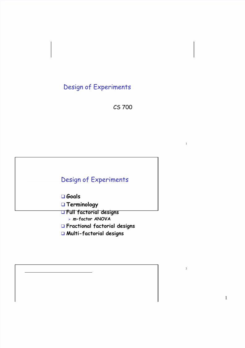
Design of Experiments

CS 700

2

Design of Experiments

Goals

Terminology

Full factorial designs m -factor ANOVA

Fractional factorial designs

Multi-factorial designs



2

3

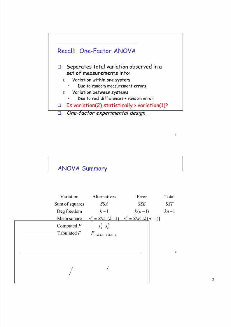
Recall: One-Factor ANOVA

Separates total variation observed in aset of measurements into:

1. Variation within one system• Due to random measurement errors

2. Variation between systems• Due to real differences + random error

Is variation(2) statistically > variation(1)?

One-factor experimental design

4

ANOVA Summary

)]1(),1(;1[

22

22

Tabulated

Computed

)]1([)1(squareMean

1)1(1freedomDeg

squaresof Sum

TotalError esAlternativVariation

!!!

!=!=

!!!

nk k

ea

ea

F F

s s F

nk SSE sk SSA s

knnk k

SST SSE SSA

"



3

5

Generalized Design of Experiments

Goals Isolate effects of each input variable.

Determine effects of interactions.

Determine magnitude of experimental error

Obtain maximum information for given effort

Basic idea Expand 1-factor ANOVA to m factors

6

Terminology

Response variable Measured output value

• E.g. total execution time

Factors Input variables that can be changed

• E.g. cache size, clock rate, bytes transmitted

Levels Specific values of factors (inputs)

• Continuous (~bytes) or discrete (type of system)



4

7

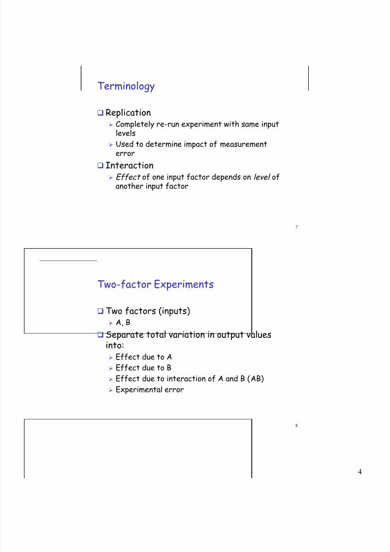
Terminology

Replication Completely re-run experiment with same input

levels

Used to determine impact of measurementerror

Interaction Effect of one input factor depends on level of

another input factor

8

Two-factor Experiments

Two factors (inputs) A, B

Separate total variation in output valuesinto: Effect due to A

Effect due to B

Effect due to interaction of A and B (AB)

Experimental error



5

9

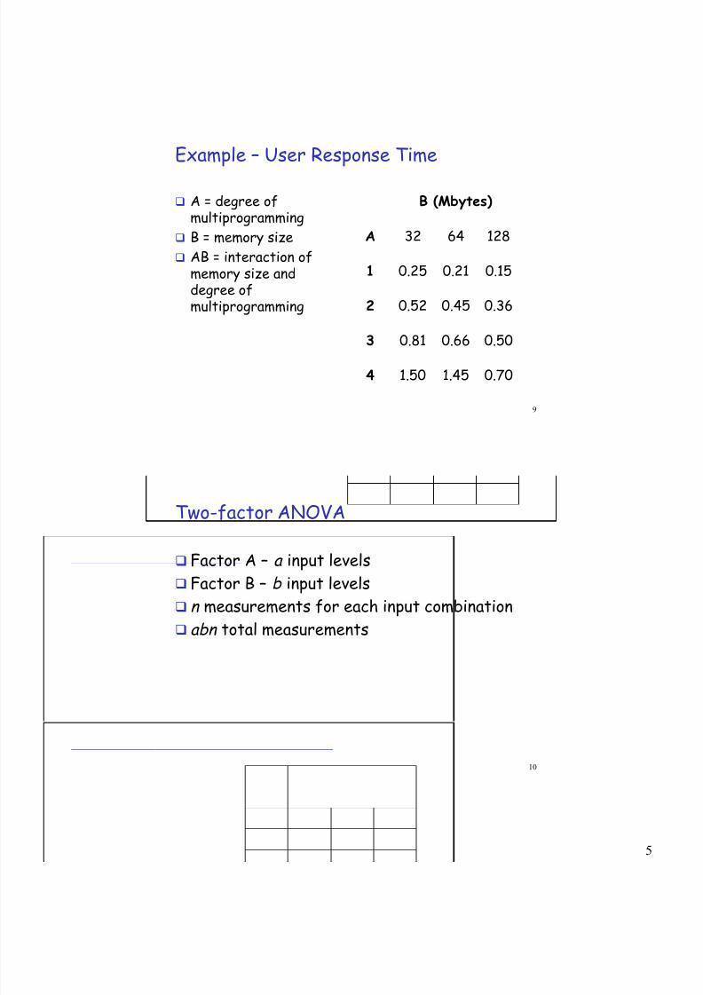
Example – User Response Time

A = degree ofmultiprogramming

B = memory size

AB = interaction ofmemory size anddegree ofmultiprogramming

0.701.451.504

0.500.660.813

0.360.450.522

0.150.210.251

1286432A

B (Mbytes)

10

Two-factor ANOVA

Factor A – a input levels

Factor B – b input levels

n measurements for each input combination

abn total measurements



6

11

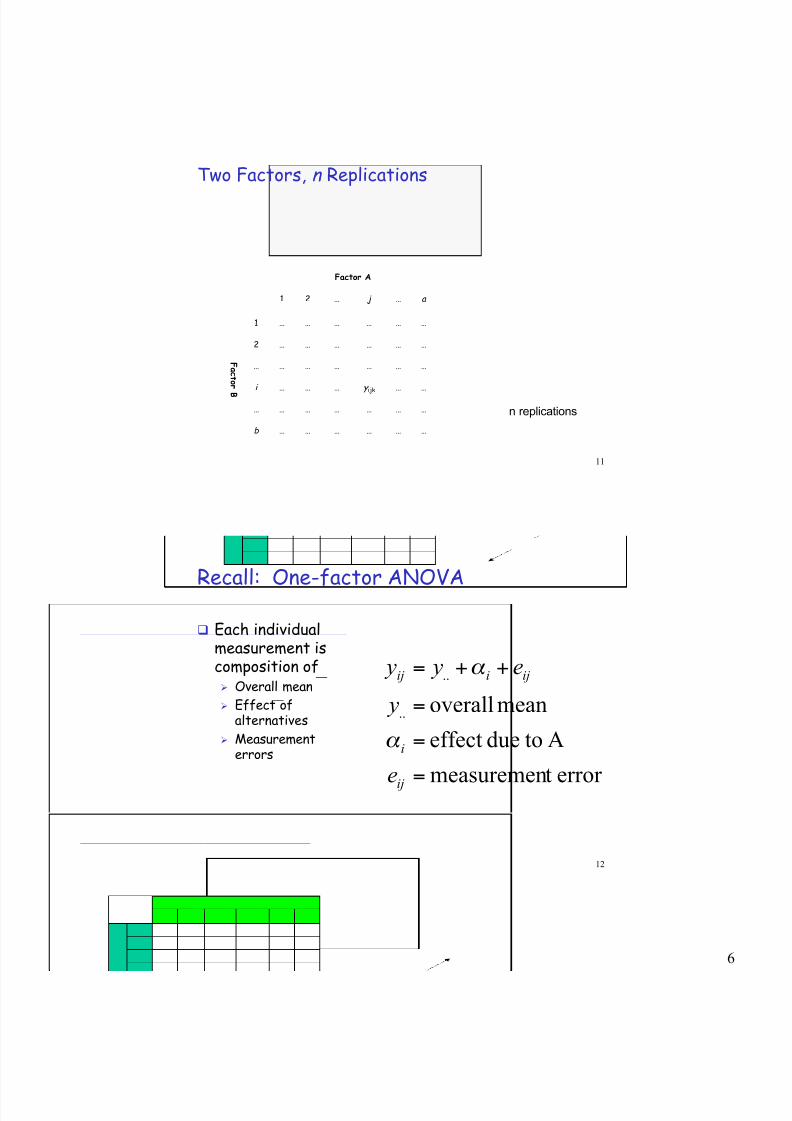
Two Factors, n Replications

F a c t o r

B

………………b

…………………

……y ijk

………i

…………………

………………2

………………1

a … j …21

Factor A

n replications

12

Recall: One-factor ANOVA

Each individualmeasurement iscomposition of Overall mean

Effect ofalternatives

Measurementerrors

error tmeasuremen

Atodueeffect

meanoverall..

..

=

=

=

++=

ij

i

ijiij

e

y

e y y

!

!



7

13

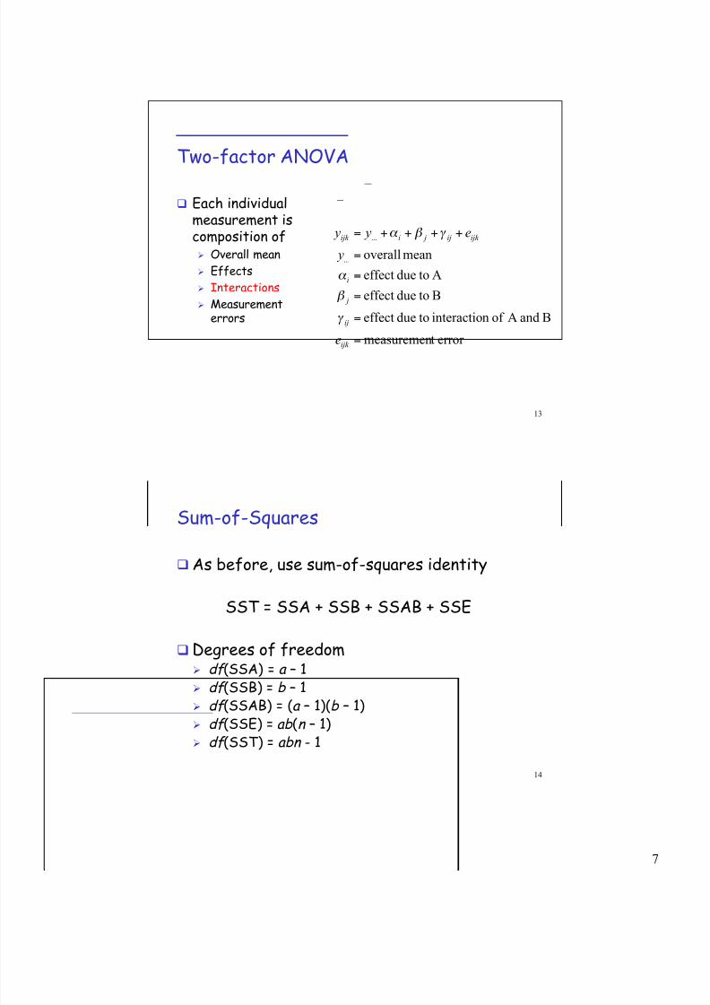
Two-factor ANOVA

Each individualmeasurement iscomposition of Overall mean

Effects

Interactions

Measurementerrors

error tmeasuremen

BandAof ninteractiotodueeffect

Btodueeffect

Atodueeffect

meanoverall...

...

=

=

=

=

=

++++=

ijk

ij

j

i

ijk ij jiijk

e

y

e y y

!

"

#

! " #

14

Sum-of-Squares

As before, use sum-of-squares identity

SST = SSA + SSB + SSAB + SSE

Degrees of freedom df (SSA) = a – 1 df (SSB) = b – 1

df (SSAB) = (a – 1)(b – 1) df (SSE) = ab (n – 1) df (SST) = abn - 1



8

15

Two-Factor ANOVA

)]1(),1)(1(;1[)]1(),1(;1[)]1(),1(;1[

222222

2222

Tabulated

Computed

)]1([)]1)(1[()1()1(squareMean

)1()1)(1(11freedomDeg

squaresof Sum

Error ABBA

!!!!!!!!!!

===

!=!!=!=!=

!!!!!

nabbanabbnaba

eababebbeaa

eabba

F F F F

s s F s s F s s F F

nabSSE sbaSSAB sbSSB saSSA s

nabbaba

SSE SSABSSBSSA

" " "

16

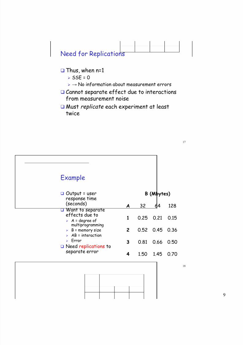
Need for Replications

If n=1 Only one measurement of each configuration

Can then be shown that SSAB = SST – SSA – SSB

Since SSE = SST – SSA – SSB – SSAB

We have SSE = 0



9

17

Need for Replications

Thus, when n=1 SSE = 0

→ No information about measurement errors

Cannot separate effect due to interactionsfrom measurement noise

Must replicate each experiment at leasttwice

18

Example Output = user

response time(seconds)

Want to separateeffects due to A = degree of

multiprogramming B = memory size AB = interaction

Error Need replications to

separate error0.701.451.504

0.500.660.813

0.360.450.522

0.150.210.251

1286432A

B (Mbytes)



10

19

Example

0.701.451.504

0.681.321.61

0.610.590.76

0.300.490.48

0.110.190.28

0.500.660.813

0.360.450.522

0.150.210.251

1286432A

B (Mbytes)

20

Example

00.389.349.3Tabulated

5.295.1052.460Computed

0024.00720.02576.01238.1squareMean

12623freedomDeg

0293.04317.05152.03714.3squaresof Sum

Error ABBA

]12,6;95.0[]12,2;95.0[]12,3;95.0[ === F F F F

F



11

21

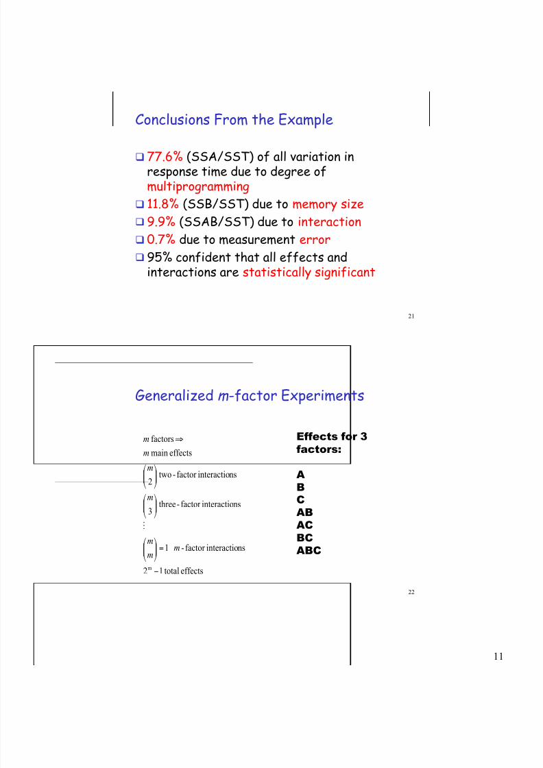
Conclusions From the Example

77.6% (SSA/SST) of all variation inresponse time due to degree ofmultiprogramming

11.8% (SSB/SST) due to memory size

9.9% (SSAB/SST) due to interaction

0.7% due to measurement error

95% confident that all effects and

interactions are statistically significant

22

Generalized m -factor Experiments

effectstotal12

nsinteractiofactor - 1

nsinteractiofactor -three3

nsinteractiofactor -two2

effectsmain

factors

m !

=""#

$%%&

'

""#

$%%&

'

""#

$%%&

'

(

m

m

m

m

m

m

m

M

Effects for 3

factors:

A

B

C

AB

AC

BCABC



12

23

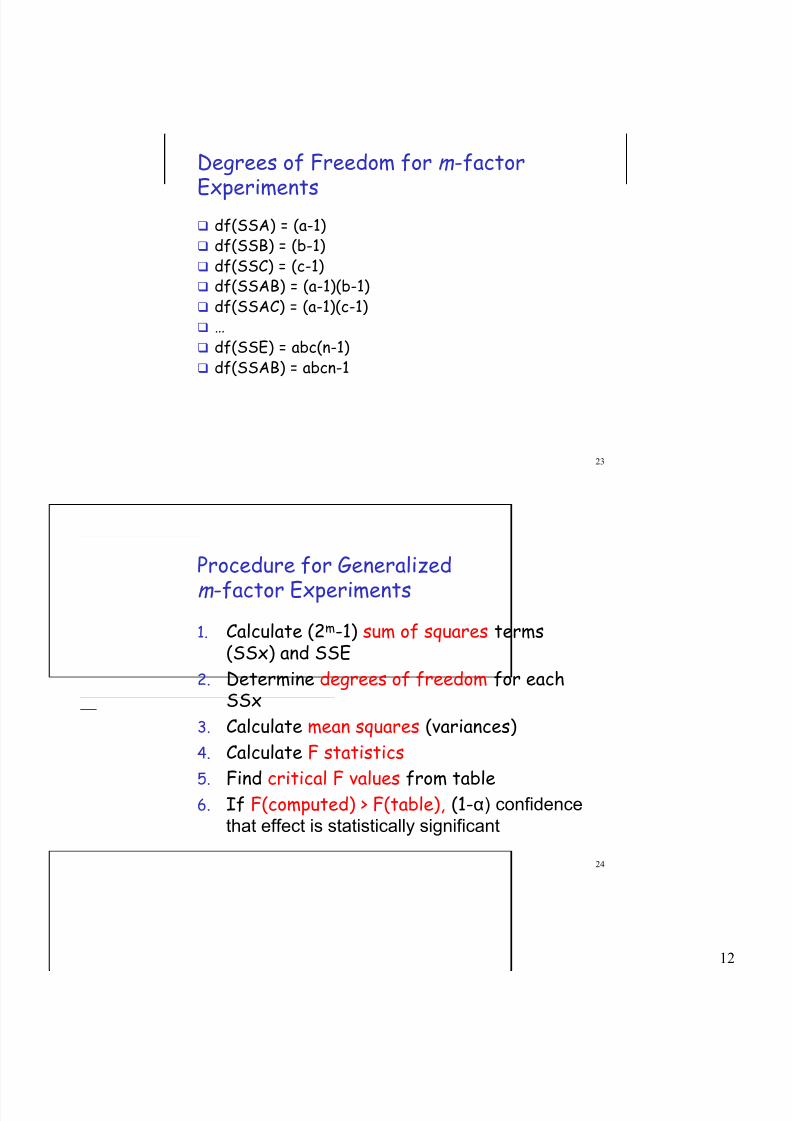
Degrees of Freedom for m -factor

Experiments df(SSA) = (a-1) df(SSB) = (b-1) df(SSC) = (c-1) df(SSAB) = (a-1)(b-1) df(SSAC) = (a-1)(c-1) … df(SSE) = abc(n-1) df(SSAB) = abcn-1

24

Procedure for Generalized

m -factor Experiments

1. Calculate (2m-1) sum of squares terms(SSx) and SSE

2. Determine degrees of freedom for eachSSx

3. Calculate mean squares (variances)

4. Calculate F statistics

5. Find critical F values from table6. If F(computed) > F(table), (1-α) confidence

that effect is statistically significant



13

25

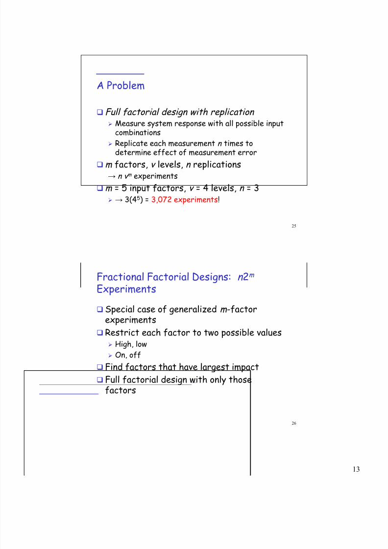
A Problem

Full factorial design with replication Measure system response with all possible input

combinations

Replicate each measurement n times todetermine effect of measurement error

m factors, v levels, n replications→ n v m experiments

m = 5 input factors, v = 4 levels, n = 3 → 3(45) = 3,072 experiments!

26

Fractional Factorial Designs: n 2m

Experiments

Special case of generalized m -factorexperiments

Restrict each factor to two possible values High, low

On, off

Find factors that have largest impact

Full factorial design with only thosefactors



14

27

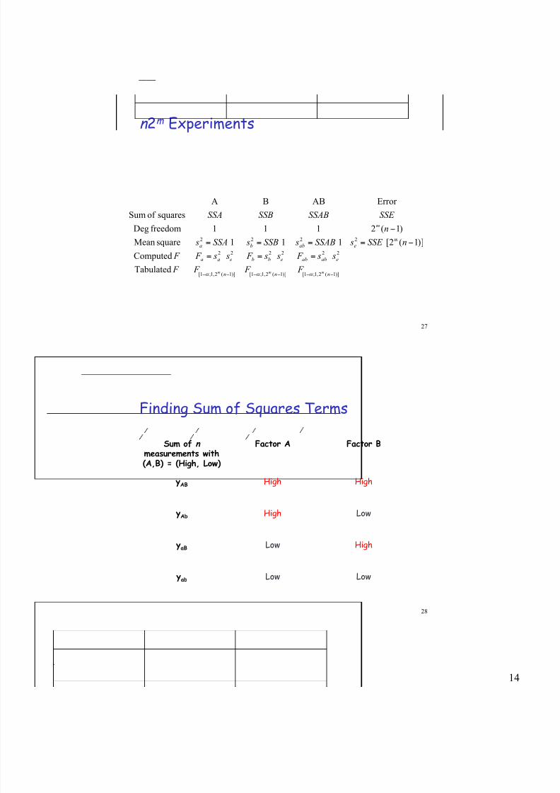
n 2m Experiments

)]1(2,1;1[)]1(2,1;1[)]1(2,1;1[

222222

2222

Tabulated

Computed

)]1(2[111squareMean

)1(2111freedomDeg

squaresof Sum

Error ABBA

!!!!!!

===

!====

!

nnn

eababebbeaa

m

eabba

m

mmm F F F F

s s F s s F s s F F

nSSE sSSAB sSSB sSSA s

n

SSE SSABSSBSSA

" " "

28

Finding Sum of Squares Terms

LowLowyab

HighLowyaB

LowHighyAb

HighHighyAB

Factor BFactor ASum of n

measurements with(A,B) = (High, Low)



15

29

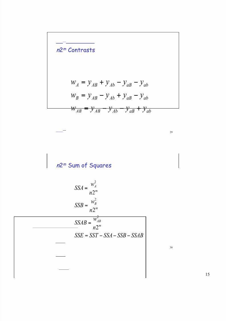
n 2m Contrasts

abaB Ab AB AB

abaB Ab AB B

abaB Ab AB A

y y y yw

y y y yw

y y y yw

+!!=

!+!=

!!+=

30

n 2m

Sum of Squares

SSABSSBSSASST SSE

n

wSSAB

n

wSSB

n

wSSA

m

AB

m

B

m

A

!!!=

=

=

=

2

2

2

2

2

2



16

31

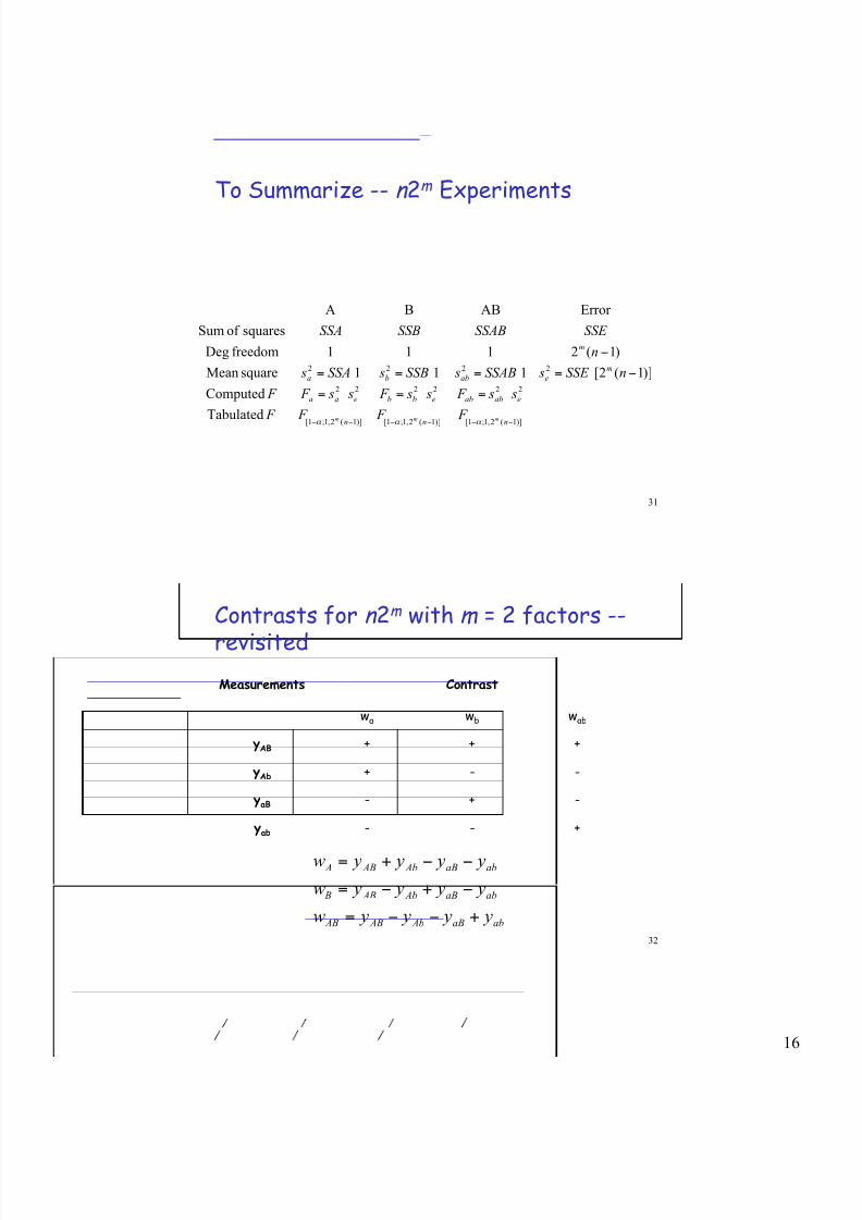
To Summarize -- n 2m Experiments

)]1(2,1;1[)]1(2,1;1[)]1(2,1;1[

222222

2222

Tabulated

Computed

)]1(2[111squareMean

)1(2111freedomDeg

squaresof Sum

Error ABBA

!!!!!!

===

!====

!

nnn

eababebbeaa

m

eabba

m

mmm F F F F

s s F s s F s s F F

nSSE sSSAB sSSB sSSA s

n

SSE SSABSSBSSA

" " "

32

Contrasts for n 2m with m = 2 factors --

revisited

wabwbwa

-

+

-

+

+-yab

--yaB

-+yAb

++yAB

ContrastMeasurements

abaB Ab AB AB

abaB Ab AB B

abaB Ab AB A

y y y yw

y y y yw

y y y yw

+!!=

!+!=

!!

+=



17

33

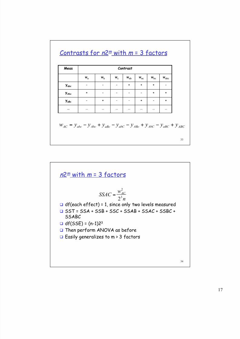
Contrasts for n 2m with m = 3 factors

…

+

+

-

wabc

…

-

+

+

wbc

…

+

-

+

wac

…

-

-

+

wabwcwbwa

…

+

-

-

………

--yaBc

-+yAbc

--yabc

ContrastMeas

ABC aBC AbC ABcabC aBc Abcabc AC y y y y y y y yw +!+!!+!=

34

n 2m

with m = 3 factors

n

wSSAC

AC

3

2

2=

df(each effect) = 1, since only two levels measured

SST = SSA + SSB + SSC + SSAB + SSAC + SSBC +SSABC

df(SSE) = (n-1)23

Then perform ANOVA as before

Easily generalizes to m > 3 factors



18

35

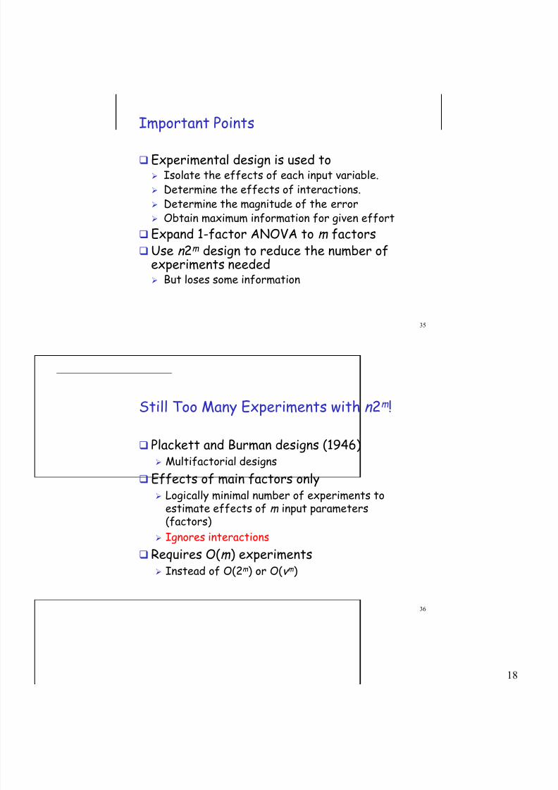
Important Points

Experimental design is used to Isolate the effects of each input variable. Determine the effects of interactions. Determine the magnitude of the error Obtain maximum information for given effort

Expand 1-factor ANOVA to m factorsUse n 2m design to reduce the number of

experiments needed But loses some information

36

Still Too Many Experiments with n 2m

!

Plackett and Burman designs (1946) Multifactorial designs

Effects of main factors only Logically minimal number of experiments to

estimate effects of m input parameters(factors)

Ignores interactions

Requires O(m ) experiments Instead of O(2m ) or O(v m )



19

37

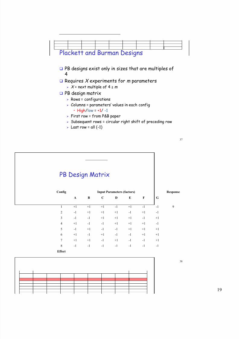
Plackett and Burman Designs

PB designs exist only in sizes that are multiples of4

Requires X experiments for m parameters X = next multiple of 4 ≥ m

PB design matrix Rows = configurations

Columns = parameters’ values in each config

• High/low = +1/ -1

First row = from P&B paper

Subsequent rows = circular right shift of preceding row

Last row = all (-1)

38

PB Design Matrix

ResponseInput Parameters (factors)Config

Effect

8

7

6

5

4

3

2

1

-1-1-1-1-1-1-1

+1-1-1+1-1+1+1

+1+1-1-1+1-1+1

+1+1+1-1-1+1-1

-1+1+1+1-1-1+1

+1-1+1+1+1-1-1

-1+1-1+1+1+1-1

9-1-1+1-1+1+1+1

GFEDCBA



20

39

PB Design Matrix


Effect

8

7

6

5

4

3

2

1

-1-1-1-1-1-1-1

+1-1-1+1-1+1+1

+1+1-1-1+1-1+1

+1+1+1-1-1+1-1

-1+1+1+1-1-1+1

+1-1+1+1+1-1-1

11-1+1-1+1+1+1-1

9-1-1+1-1+1+1+1

GFEDCBA

40

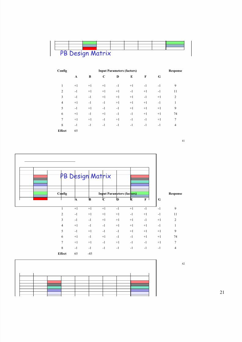
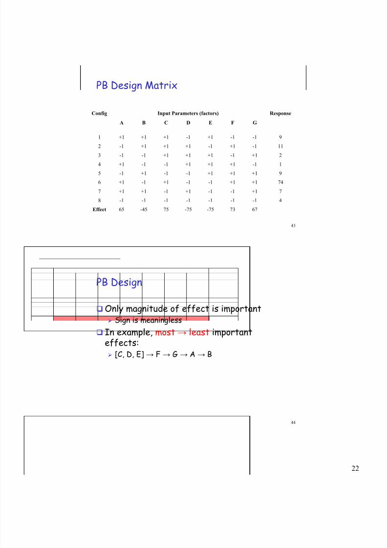
PB Design Matrix


Effect

8

7

6

5

4

3

2

1

4-1-1-1-1-1-1-1

7+1-1-1+1-1+1+1

74+1+1-1-1+1-1+1

9+1+1+1-1-1+1-1

1-1+1+1+1-1-1+1

2+1-1+1+1+1-1-1

11-1+1-1+1+1+1-1

9-1-1+1-1+1+1+1

GFEDCBA



21

41

PB Design Matrix


Effect

8

7

6

5

4

3

2

1

65

4-1-1-1-1-1-1-1

7+1-1-1+1-1+1+1

74+1+1-1-1+1-1+1

9+1+1+1-1-1+1-1

1-1+1+1+1-1-1+1

2+1-1+1+1+1-1-1

11-1+1-1+1+1+1-1

9-1-1+1-1+1+1+1

GFEDCBA

42

PB Design Matrix


Effect

8

7

6

5

4

3

2

1

-4565

4-1-1-1-1-1-1-1

7+1-1-1+1-1+1+1

74+1+1-1-1+1-1+1

9+1+1+1-1-1+1-1

1-1+1+1+1-1-1+1

2+1-1+1+1+1-1-1

11-1+1-1+1+1+1-1

9-1-1+1-1+1+1+1

GFEDCBA



22

43

PB Design Matrix


Effect

8

7

6

5

4

3

2

1

6773-75-7575-4565

4-1-1-1-1-1-1-1

7+1-1-1+1-1+1+1

74+1+1-1-1+1-1+1

9+1+1+1-1-1+1-1

1-1+1+1+1-1-1+1

2+1-1+1+1+1-1-1

11-1+1-1+1+1+1-1

9-1-1+1-1+1+1+1

GFEDCBA

44

PB Design

Only magnitude of effect is important Sign is meaningless

In example, most → least importanteffects: [C, D, E] → F → G → A → B



23

45

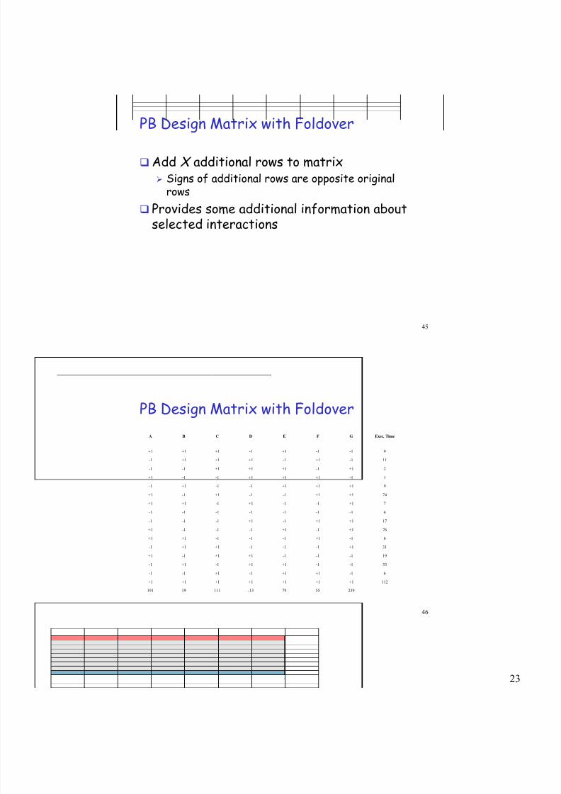
PB Design Matrix with Foldover

Add X additional rows to matrix Signs of additional rows are opposite original

rows

Provides some additional information aboutselected interactions

46

PB Design Matrix with Foldover

2395579-1311119191

112+1+1+1+1+1+1+1

6-1+1+1-1+1-1-1

33-1-1+1+1-1+1-1

19-1-1-1+1+1-1+1

31+1-1-1-1+1+1-1

6-1+1-1-1-1+1+1

76+1-1+1-1-1-1+1

17+1+1-1+1-1-1-1

4-1-1-1-1-1-1-1

7+1-1-1+1-1+1+1

74+1+1-1-1+1-1+1

9+1+1+1-1-1+1-1

1-1+1+1+1-1-1+1

2+1-1+1+1+1-1-1

11-1+1-1+1+1+1-1

9-1-1+1-1+1+1+1

Exec. TimeGFEDCBA



24

47

Case Study #1

Determine the most significant parameters in aprocessor simulator.

[Yi, Lilja, & Hawkins, HPCA, 2003.]

48

Determine the Most Significant

Processor Parameters

Problem So many parameters in a simulator How to choose parameter values? How to decide which parameters are most

important?

Approach

Choose reasonable upper/lower bounds. Rank parameters by impact on total execution

time.



25

49

Simulation Environment

SimpleScalar simulator sim-outorder 3.0

Selected SPEC 2000 Benchmarks gzip, vpr, gcc, mesa, art, mcf, equake, parser, vortex, bzip2,

twolf

MinneSPEC Reduced Input Sets Compiled with gcc (PISA) at O3

50

Functional Unit Values

Equal to Int Div LatencyInt Div Throughput

41FP Mult/Div Units

2 Cycles5 CyclesFP Mult Latency

10 Cycles35 CyclesFP Div Latency

10 Cycles80 CyclesInt Div Latency

1Int Mult Throughput

15 Cycles35 CyclesFP Sqrt Latency

2 Cycles

41Int Mult/Div Units

15 CyclesInt Mult Latency

Equal to FP Sqrt LatencyFP Sqrt Throughput

Equal to FP Div LatencyFP Div Throughput

Equal to FP Mult LatencyFP Mult Throughput

1FP ALU Throughputs

1 Cycle5 CyclesFP ALU Latency

41FP ALUs

1Int ALU Throughput

1 Cycle2 CyclesInt ALU Latency

41Int ALUs

High ValueLow ValueParameter



26

51

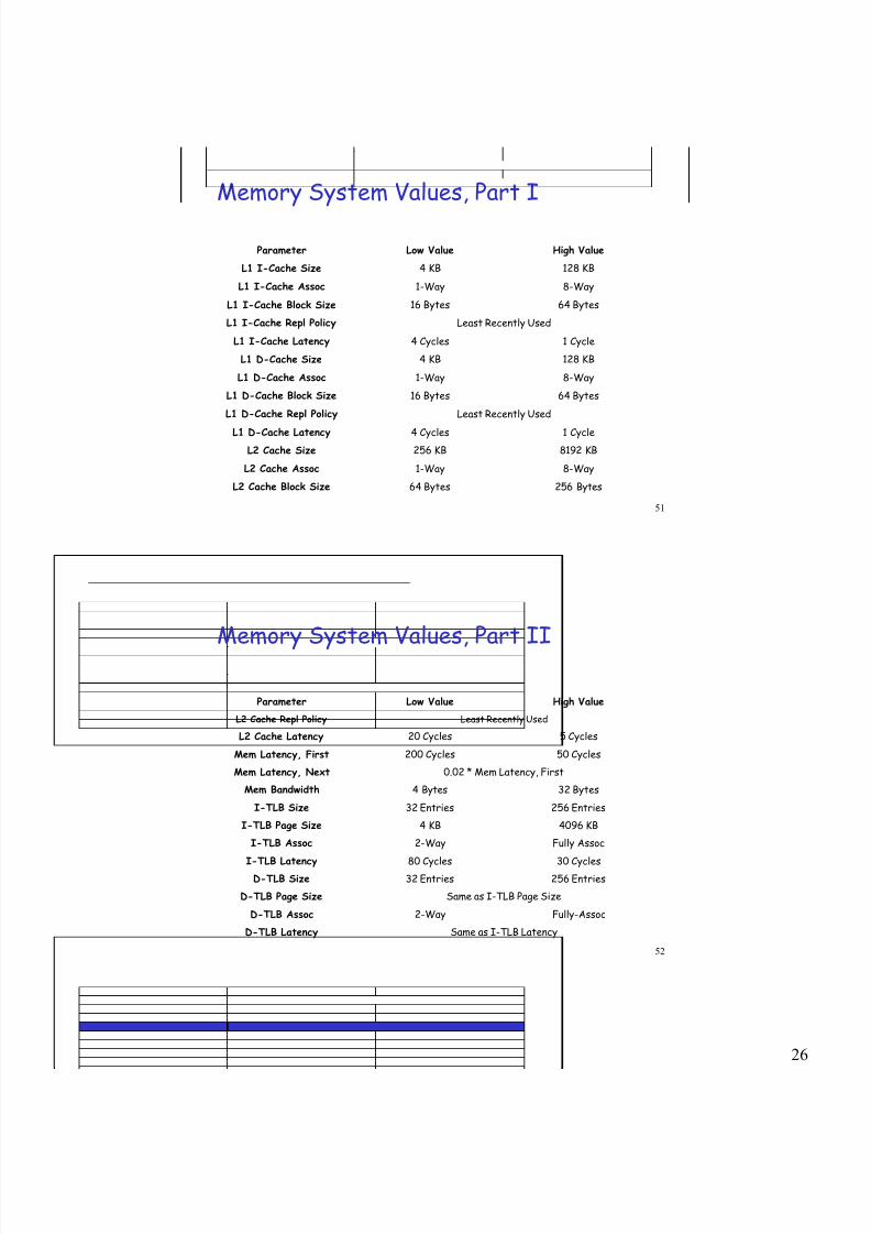
Memory System Values, Part I

8192 KB256 KBL2 Cache Size1 Cycle4 CyclesL1 D-Cache Latency

Least Recently UsedL1 D-Cache Repl Policy

64 Bytes16 BytesL1 D-Cache Block Size

8-Way1-WayL1 D-Cache Assoc

128 KB4 KBL1 D-Cache Size

1 Cycle4 CyclesL1 I-Cache Latency

Least Recently UsedL1 I-Cache Repl Policy

256 Bytes64 BytesL2 Cache Block Size

8-Way1-WayL2 Cache Assoc

64 Bytes16 BytesL1 I-Cache Block Size

8-Way1-WayL1 I-Cache Assoc

128 KB4 KBL1 I-Cache Size


52

Memory System Values, Part II

Least Recently UsedL2 Cache Repl Policy

Fully-Assoc

256 Entries32 EntriesI-TLB Size

4096 KB4 KBI-TLB Page Size

Fully Assoc2-WayI-TLB Assoc

30 Cycles80 CyclesI-TLB Latency

0.02 * Mem Latency, FirstMem Latency, Next

32 Bytes4 BytesMem Bandwidth

256 Entries32 EntriesD-TLB Size

50 Cycles

5 Cycles20 CyclesL2 Cache Latency

200 CyclesMem Latency, First

Same as I-TLB LatencyD-TLB Latency

2-WayD-TLB Assoc

Same as I-TLB Page SizeD-TLB Page Size




27

53

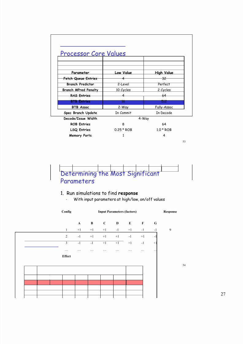
Processor Core Values

In DecodeIn CommitSpec Branch Update

4-WayDecode/Issue Width

41Memory Ports

1.0 * ROB0.25 * ROBLSQ Entries

648ROB Entries

Fully-Assoc2-WayBTB Assoc

51216BTB Entries

644RAS Entries

2 Cycles10 CyclesBranch MPred Penalty

Perfect2-LevelBranch Predictor

324Fetch Queue Entries


54

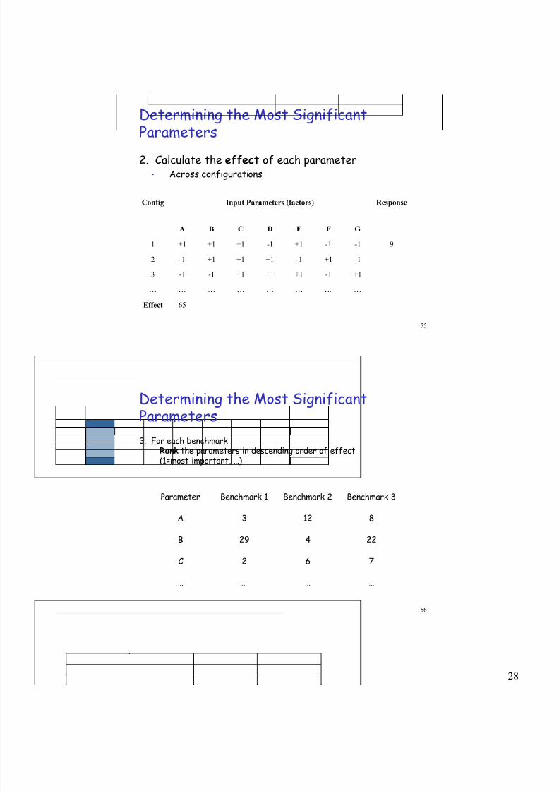
Determining the Most Significant

Parameters

1. Run simulations to find response• With input parameters at high/low, on/off values


Effect

…

3

2

1

…………………

+1-1+1+1+1-1-1

-1+1-1+1+1+1-1

9-1-1+1-1+1+1+1

GFEDCBA



28

55


Parameters2. Calculate the effect of each parameter

• Across configurations


Effect

…

3

2

1

65

…………………

+1-1+1+1+1-1-1

-1+1-1+1+1+1-1

9-1-1+1-1+1+1+1

GFEDCBA

56


Parameters3. For each benchmark

Rank the parameters in descending order of effect(1=most important, …)

…………

762C

22429B

8123A

Benchmark 3Benchmark 2Benchmark 1Parameter



29

57


Parameters4. For each parameter

Average the ranks

……………

5

18.3

7.67

Average

762C

22429B

8123A

Benchmark 3Benchmark 2Benchmark 1Parameter

58

Most Significant Parameters

18.23

12.62

12.31

11.77

10.62

10.23

10.00

9.08

7.69

4.00

2.77

Average

28

10

9

3

6

1

7

8

5

2

4

gcc

11

10

9

8

7

6

5

4

3

2

1

Number

8

12

36

16

9

6

7

3

2

4

1

gzip

16

39

3

10

1

12

8

29

27

4

2

art

L2 Cache Size

Branch Predictor Accuracy

Speculative Branch Update

LSQ Entries

Memory Latency, First

L1 I-Cache Block Size

L1 I-Cache Size

L1 D-Cache Latency

Number of Integer ALUs

L2 Cache Latency

ROB Entries

Parameter



30

59

General Procedure

Determine upper/lower bounds forparameters

Simulate configurations to find response Compute effects of each parameter for

each configuration Rank the parameters for each benchmark

based on effectsAverage the ranks across benchmarks Focus on top-ranked parameters for

subsequent analysis

60

Case Study #2

Determine the “big picture” impact of a systemenhancement.



31

61

Determining the Overall Effect of an

Enhancement

Problem: Performance analysis is typically limited to single

metrics• Speedup, power consumption, miss rate, etc.

Simple analysis• Discards a lot of good information

62

Determining the Overall Effect of an

Enhancement

Find most important parameters withoutenhancement Using Plackett and Burman

Find most important parameters withenhancement Again using Plackett and Burman

Compare parameter ranks



32

63

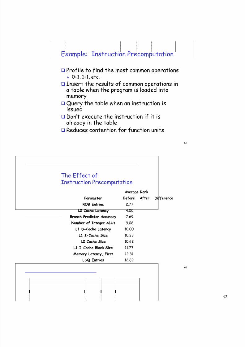
Example: Instruction Precomputation

Profile to find the most common operations 0+1, 1+1, etc.

Insert the results of common operations ina table when the program is loaded intomemory

Query the table when an instruction isissued

Don’t execute the instruction if it isalready in the table

Reduces contention for function units

64

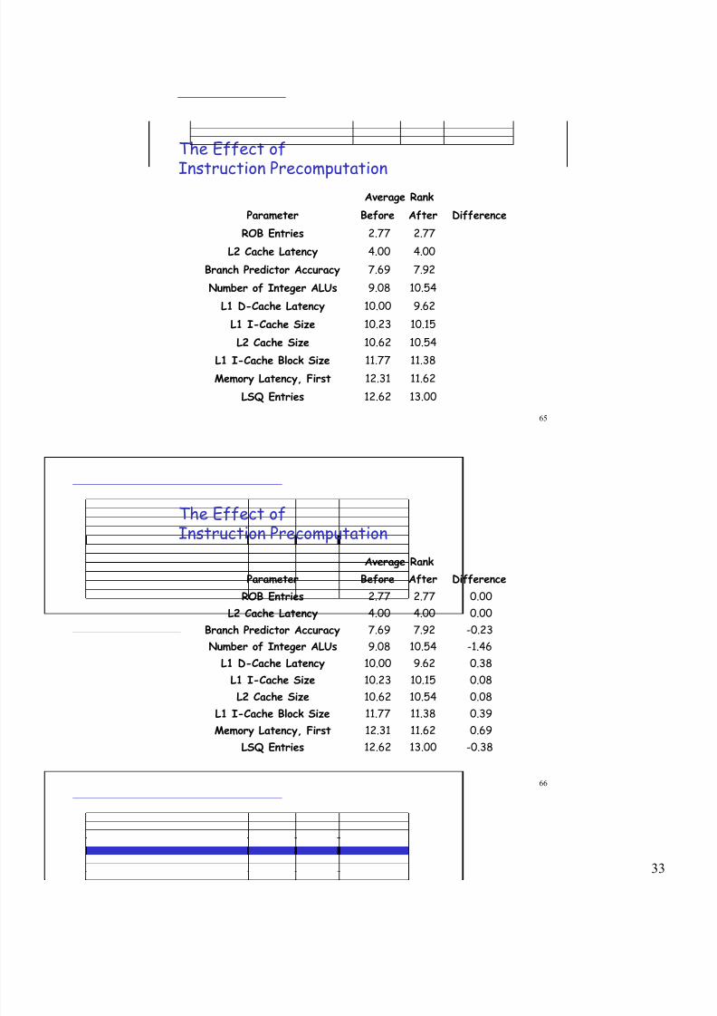
The Effect of

Instruction PrecomputationAverage Rank

After Difference

LSQ Entries


L1 I-Cache Block SizeL2 Cache Size

L1 I-Cache Size

L1 D-Cache Latency



L2 Cache Latency

ROB Entries

Parameter

12.62

12.31

11.7710.62

10.23

10.00

9.08

7.69

4.00

2.77

Before



33

65

The Effect of


13.00

11.62

11.38

10.54

10.15

9.62

10.54

7.92

4.00

2.77

After Difference

LSQ Entries



L2 Cache Size

L1 I-Cache Size

L1 D-Cache Latency



L2 Cache Latency

ROB Entries

Parameter

12.62

12.31

11.77

10.62

10.23

10.00

9.08

7.69

4.00

2.77

Before

66

The Effect of


13.00

11.6211.38

10.54

10.15

9.62

10.54

7.92

4.00

2.77

After

-0.38

0.690.39

0.08

0.08

0.38

-1.46

-0.23

0.00

0.00

Difference

LSQ Entries

Memory Latency, FirstL1 I-Cache Block Size

L2 Cache Size

L1 I-Cache Size

L1 D-Cache Latency



L2 Cache Latency

ROB Entries

Parameter

12.62

12.3111.77

10.62

10.23

10.00

9.08

7.69

4.00

2.77

Before



34

67

Case Study #3

Benchmark program classification.

68

Benchmark Classification

By application type Scientific and engineering applications Transaction processing applications Multimedia applications

By use of processor function units Floating-point code Integer code

Memory intensive code Etc., etc.



35

69

Another Point-of-View

Classify by overall impact on processor

Define: Two benchmark programs are similar if –

• They stress the same components of a system tosimilar degrees

How to measure this similarity? Use Plackett and Burman design to find ranks

Then compare ranks

70

Similarity metric

Use rank of each parameter as elements ofa vector

For benchmark program X, let X = (x1, x2,…, xn-1, xn)

x1 = rank of parameter 1

x2 = rank of parameter 2

…



36

71

Vector Defines a Point in

n -space

• (y1, y2, y3)

Param #3

• (x1, x2, x3)

Param #2

Param #1

D

72

Similarity Metric

Euclidean Distance Between Points

2/122

11

2

22

2

11 ])()()()[( nnnn y x y x y x y x D !+!++!+!=!!

K



37

73

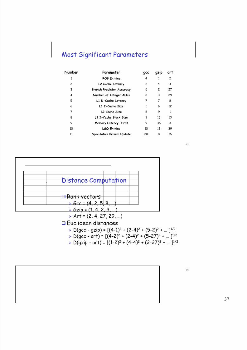
Most Significant Parameters

28

10

9

3

6

1

7

8

5

2

4

gcc

11

10

9

8

7

6

5

4

3

2

1

Number

8

12

36

16

9

6

7

3

2

4

1

gzip

16

39

3

10

1

12

8

29

27

4

2

art

L2 Cache Size


Speculative Branch Update

LSQ Entries



L1 I-Cache Size

L1 D-Cache Latency


L2 Cache Latency

ROB Entries

Parameter

74

Distance Computation

Rank vectors Gcc = (4, 2, 5, 8, …) Gzip = (1, 4, 2, 3, …) Art = (2, 4, 27, 29, …)

Euclidean distances D(gcc - gzip) = [(4-1)2 + (2-4)2 + (5-2)2 + … ]1/2

D(gcc - art) = [(4-2)2 + (2-4)2 + (5-27)2 + … ]1/2

D(gzip - art) = [(1-2)2

+ (4-4)2

+ (2-27)2

+ … ]1/2



38

75

Euclidean Distances for Selected

Benchmarks

0mcf

98.6

109.6

94.5

mcf

0art

113.50gzip

92.681.90gcc

artgzipgcc

76

Dendogram of Distances Showing (Dis-

)Similarity



39

77

Final Benchmark Groupings

ammpVIII

EquakeVIIMcfVI

ArtV

Gcc, vortexIV

Vpr-Route, parser, bzip2III

Vpr-Place,twolfII

Gzip,mesaI

BenchmarksGroup

78

Important Points

Multifactorial (Plackett and Burman) design Requires only O(m ) experiments

Determines effects of main factors only

Ignores interactions

Logically minimal number of experiments toestimate effects of m input parameters

Powerful technique for obtaining a big-picture view of a lot of data



40

79

Summary

Design of experiments

Isolate effects of each input variable.

Determine effects of interactions.

Determine magnitude of experimental error

m -factor ANOVA (full factorial design )

All effects, interactions, and errors

80

Summary

n2m designs Fractional factorial design

All effects, interactions, and errors

But for only 2 input values high/low

on/off



81

Summary

Plackett and Burman (multi-factorial design )

O(m ) experiments

Main effects only No interactions

For only 2 input values (high/low, on/off)

Examples – rank parameters, group

benchmarks, overall impact of anenhancement

doe lecture 10

Documents