does exchange rate regime explain differences in economic
TRANSCRIPT

No 2004 – 05May
Does Exchange Rate Regime Explain Differences inEconomic Results for Asian Countries ?
_____________
Virginie CoudertMarc Dubert
CEPII, Working Paper No 2003 -05
2
Does Exchange Rate Regime Explain Differences inEconomic Results for Asian Countries ?
_____________
Virginie CoudertMarc Dubert
No 2004 – 05May

Does Exchange Rate Regime Explain Differences in Economic Results for Asian Countries ?
3
TABLE OF CONTENTS
SUMMARY..............................................................................................................................................4
ABSTRACT..............................................................................................................................................4
RÉSUMÉ..................................................................................................................................................6
RÉSUMÉ COURT....................................................................................................................................7
1. INTRODUCTION ...........................................................................................................................8
2. HOW TO CLASSIFY? DRAWING LESSONS FROM THE LITERATURE....................................9
3. THE CLASSIFICATION METHODUSED IN THIS STUDY.........................................................14
4. CLASSIFICATION RESULTS ......................................................................................................21
5. ECONOMETRIC ANALYSIS .......................................................................................................26
6. CONCLUSION..............................................................................................................................34
BIBLIOGRAPHY...................................................................................................................................36
APPENDIX.............................................................................................................................................40
LIST OF WORKING PAPERS RELEASED BY CEPII ..........................................................................48

CEPII, Working Paper No 2003 -05
4
DOES EXCHANGE RATE REGIME EXPLAIN DIFFERENCES IN ECONOMIC RESULTSFOR ASIAN COUNTRIES ?
SUMMARY
The paper aims at determining whether exchange rate regimes have an impact on inflationand growth, on a sample of ten major Asian countries for the period 1990:1-2001:4.
First, we review the main existing de facto classifications for exchange rate regimes andfind some features that could distort results. For example, in the most famous one, byLevy-Yeyati and Sturzenegger, (2000, 2003), in addition to the number of inconclusiveobservations, ruptures of anchorage are not identified and mostly classified as floats, whichmakes the “float” category not really relevant. This caveat is solved in the “naturalclassification” by Calvo and Reihnart (2003). However, this classification does not takeinto account the central banks’ behaviour on the forex market, which can be important todiscriminate between “managed float” and “float”.
Secondly, we propose a new statistical method for identifying de facto exchange rateregimes: observations are classified into four categories: float, managed float, crawling pegand peg. We take stock of the results of Bénassy-Quéré and Coeuré (2000), evidencing thedollar as the main anchor currency in the Asian countries. The procedure includes severalsteps: successively taking into account the trends in the exchange rate levels in order toseparate crawling pegs from pegs, comparing the variances in the exchange rates and forexreserves changes to the ones of a benchmark sample of floating currencies. More precisely,we calculate quarterly variances of exchange rates using weekly data and carry out a Fishertest for comparing this variance to the one calculated on a benchmark sample of floatingcurrencies: USD/DEM-EUR, USD/JPY and USD/GBP. We perform the same kind of testfor forex reserves to discriminate between float and managed float. In a final stage,devaluation periods are identified, on the basis of quarterly trend of depreciation. Thismethod yields quarterly results that are checked to be consistent with common knowledge:most South Asian countries had de facto pegs before the Asian crisis and let their currencyfloat afterwards.
Thirdly, we use this classification for assessing the effects of exchange rates regimes oninflation and growth. We perform pooled regressions with lagged exchange rate regimesdummies and several control variables. Results show that pegs are associated with weakergrowth and lower inflation. However, results on inflation are questionable, as anendogeneity bias is not excluded.
ABSTRACT
The paper aims at determining whether exchange rate regimes have an impact on inflationand growth for a sample of ten major Asian countries for the period 1990:01-2001:04.First, we try to improve upon existing de facto classifications and propose a new statisticalmethod for identifying de facto exchange rate regimes: observations are classified into fourcategories: float, managed float, crawling peg and peg. The procedure includes severalsuccessive steps: taking into account the trends in the exchange rate levels, comparing the

Does Exchange Rate Regime Explain Differences in Economic Results for Asian Countries ?
5
variances in the exchange rates and forex reserves changes to a benchmark sample offloating currencies. Devaluation periods are also identified. This method yields quarterlyresults that are checked to be consistent with common knowledge. Second, we use thisclassification for assessing the effects of exchange rates regimes on inflation and growth.We perform pooled regressions with lagged exchange rate regimes dummies and severalcontrol variables. Results show that pegs are associated with weaker growth than floatingexchange rate regimes. Results on inflation are more questionable, as an endogeneity biasis not excluded.
J.E.L. classification: F33Keywords: Exchange rate regime, Economic performance, Asian countries

CEPII, Working Paper No 2003 -05
6
LES RÉGIMES DE CHANGE ONT-ILS UNE INFLUENCE SUR LES PERFORMANCESÉCONOMIQUES DES PAYS ASIATIQUES ?
RÉSUMÉ
Le but de cette étude est de déterminer si les régimes de change ont un impact surl’inflation et la croissance sur un échantillon de dix pays asiatiques pour la période1990:01-2001:04. Premièrement, nous passons en revue les méthodes de classificationsexistantes et identifions un certain nombre de caractéristiques qui peuvent biaiser lesrésultats. Par exemple, dans la classification fameuse de Levy-Yeyati and Sturzenegger,(2000, 2003), en plus du nombre important d’observations sur lesquelles la méthode nepeut conclure, les ruptures d’ancrage ne sont pas identifiées. En conséquence, cesobservations sont souvent classées à tort dans la catégorie « flottement », ce qui rend cettecatégorie peu pertinente. Ce travers ne se retrouve pas dans la classification de Calvo andReihnart (2003) . Cependant, cette méthode ne prend pas en compte les interventions desbanques centrales sur le marché des changes, pourtant décisives pour distinguer entre lesflottements gérés et les flottements purs.
Deuxièmement, nous proposons une nouvelle méthode statistique pour identifier lesrégimes de change de facto : les observations sont classées en quatre catégories: taux dechange flottants, flottement géré, taux de change fixes et à parités glissantes. Nous nousappuyons sur les résultats obtenus par Bénassy-Quéré and Coeuré (2000), qui mettent enévidence l’ancrage des monnaies asiatiques sur le dollar. La procédure mise en œuvrecomporte plusieurs étapes successives: la prise en en compte des tendances des taux dechanges – afin de départager les taux de changes fixes des parités glissantes - ; lacomparaison des variances des taux de change et des réserves officielles avec celles d’unéchantillon de référence composé de monnaies flottantes. Plus précisément, nous calculonsdes variances trimestrielles des taux de change en utilisant des données hebdomadaires etfaisons un test de Fisher pour comparer les variances obtenues pour chaque pays asiatique àcelles d’un échantillon de référence composé de monnaies que nous considérons commeflottantes : USD/DEM-EUR, USD/JPY et USD/GBP. Nous procédons au même test en cequi concerne les réserves officielles pour séparer les flottements des flottements gérés. Dansune étape finale, nous identifions les périodes de dévaluation sur la base de la tendancetrimestrielle. La méthode donne des résultats qui permettent de retrouver les faits stylisés,mis en évidence dans les études sur la question : la plupart des pays asiatiques avaient desrégimes de change fixes de facto avant la crise de 1997 et ont laissé flotter leur monnaieensuite.
Troisièmement, nous utilisons cette classification pour évaluer les effets des régimes dechange sur l’inflation et la croissance. Pour cela, nous faisons des régressions empilées avecdes variables muettes représentant les régimes de change et des variables de contrôle. Lesrésultats montrent que les taux de change fixes sont associés à une croissance plus faibleque les changes flottants. L’effet sur le taux de croissance persiste après correction d’unbiais éventuel d’endogénéité. Les résultats sur l’inflation sont moins tranchés car un biaisd’éndogénéité n’est pas exclu.

Does Exchange Rate Regime Explain Differences in Economic Results for Asian Countries ?
7
RÉSUMÉ COURT
Le but de cette étude est de déterminer si les régimes de change ont un impact surl’inflation et la croissance sur un échantillon de dix pays asiatiques pour la période1990:01-2001:04. Premièrement, nous essayons d’améliorer les classifications existantes enproposant une nouvelle méthode statistique pour identifier les régimes de change de facto :les observations sont classées en quatre catégories: taux de change flottants, flottementgéré, taux de change fixes et à parités glissantes. La procédure mise en œuvre comporteplusieurs étapes successives: la prise en en compte des tendances des taux de changes, lacomparaison des variances des taux de change et des réserves officielles à celles d’unéchantillon de référence composé de monnaies flottantes. Deuxièmement, nous utilisonscette classification pour évaluer les effets des régimes de change sur l’inflation et lacroissance. Pour cela, nous faisons des régressions empilées avec des variables muettesreprésentant les régimes de change et des variables de contrôle. Les résultats montrent queles taux de change fixes sont associés à une croissance plus faible que les changes flottants.Les résultats sur l’inflation sont moins tranchés car un biais d’éndogénéité ne peut êtreexclu.
J.E.L.: F33Mots-clés: régime de change, performance économique, Asie
CEPII, Working Paper No 2003 -05
8
DOES EXCHANGE RATE REGIME EXPLAIN DIFFERENCES IN ECONOMIC RESULTSFOR ASIAN COUNTRIES ? 1
Virginie Coudert 2 and Marc Dubert
3
1. INTRODUCTION
The exchange rate regime is one of the central choice of the economic policy. However,the debate over fixed-versus-floating systems has often been muddied by therecommendations of the International Monetary Fund (IMF), which have shifted accordingto circumstances. In the wake of the 1997 Asian crisis, the IMF accused “soft” pegs, notreally of playing a part in the Asian meltdown, but of amplifying the cost of the crisis. It istrue that pegged exchange rates encouraged growth in unhedged foreign-currency debt andcurrency mismatch of balance-sheets. This pushed up the costs of devaluation forborrowers, triggering chains of business and bank failures. These events, together with themassive losses incurred by the monetary authorities as they sought to defend their exchangerates from speculative attack, resulted in an even higher bill for the crisis resolution and,hence, played a role in the ensuing IMF’s doctrinal shift. Having long supported fixedexchange rate regimes as a weapon in the fight against inflation, the IMF turned to “corner”solutions, based on hard pegs - currency boards or dollarisation - or pure floats, in the latenineties (Fischer, 2001). However, there was another shift of doctrine, after the Argentinecrisis in 2001-2002. Since that time, the IMF has stopped recommending currency boardsas a credible solution and has switched to its current doctrine of floating arrangements withinflation targeting (Rogoff and alii, 2003). Such changes in recommendations show thegreat uncertainty, that still undermines this issue.
Accordingly, the debate must be recast to include research that analyses countries'macroeconomic performances according to their exchange rate regime and get ridded ofpartisan considerations. In theory, the nominal regime should be able to influence inflation,by creating an external anchor for the currency, and thus have a neutral impact on long-term growth. But if the risks of crisis are increased by keeping rates fixed for too long,macroeconomic performance is likely to be affected.
To briefly sum up this long debate, let us go back to Obsfeld and Rogoff (1995), whosearticle, “The Mirage of Fixed Exchange Rates”, warns against fixed regimes. Their paperargues that such systems last on average for a couple of years and are regularly followed bya collapse in the exchange rate and a currency crisis. In countries with stubborn inflation, a
1 We thank Agnès Bénassy-Quéré and Francisco Serranito for helpful comments on a first draft of this
paper. We also thank participants of the internal seminar of the CEPN, University of Paris 13, where a firstversion of the paper was presented in June 2003, especially Jacques Mazier and Dominique Plihon, for theirremarks. We are also grateful to participants of the conference on “Econometrics of Emerging Markets”organised by the Applied Econometric Association in November 2003. The opinions expressed are those ofthe authors and do not reflect the view of institutions they belong to.2 Banque de France, CEPII and University Paris 13, CEPN , CNRS-UMR7115
3 University Paris 13, CEPN , CNRS-UMR7115

Does Exchange Rate Regime Explain Differences in Economic Results for Asian Countries ?
9
fixed exchange rate often causes the real exchange rate to become overvalued. This turnsout to be unsustainable in the medium term, leaving the regime vulnerable to speculativeattack. Williamson (2000) therefore recommends making fixed exchange rate regimes moreflexible by introducing soft crawling bands pegged to currency baskets. In her famousarticle, “The Mirage of Floating Exchange Rates”, Reinhart (2000) says that floating ratesare even more of a delusion than fixed ones, for the simple reason that they do not exist.Looking at a large sample of countries, she demonstrates that no emerging country actuallyallows its exchange rate to float, because the governments of these countries suffer fromwhat Calvo and Reinhart (2002) dubbed the “fear of floating”. This subject has spawned anample literature. But in the end, few empirical studies have considered the issue of howexchange rate regimes affect countries’ economic performances. To our knowledge, theonly existing studies to offer a statistical analysis of this question are those commissionedby the IMF: Ghosh and alii (1997) and Levy-Yeyati and Sturzenegger (2001), Rogoff andalii (2003).
In this paper, we have focused on a sample of ten Asian countries – China, South Korea,Hong Kong, India, Indonesia, Malaysia, Pakistan, the Philippines, Singapore and Thailand– over the period 1990-2001. This sample is of particular interest, for several reasons.First, these countries employed a diverse array of exchange rate systems during the periodunder review. Second, they share common characteristics that facilitate a comparativeanalysis. Third, the crisis that marked this period allows to test the vulnerability ofdifferent regimes to speculative attacks.
An important preliminary stage of this study was to identify the "de facto" exchange rateregimes in each country. The recent literature contains several methods for this, notablythose of Calvo and Reinhart (2002), and Levy-Yeyati and Sturzenegger (2000, 2003).However, having conducted a critical examination of these methods, we opted to constructone of our own, explained in detail below. The second stage consisted in performing aneconometric analysis of the macroeconomic performances of countries according to theiridentified exchange rate regime. We concentrate on the results in terms of growth andinflation.
The rest of this paper is organised as follows. Section two describes the methods used inthe economic literature to identify the de facto regimes actually in use in different countries.Section three explains and justifies our method. Section four sets out the findings andcompares them with those of the other available studies. Section five consists of aneconometric analysis of the effects of exchange rate regimes. Section six concludes.
2. HOW TO CLASSIFY? DRAWING LESSONS FROM THE LITERATURE
Several studies were carried out in the early 1990s with the aim of identifying "de facto"exchange rate regimes. Two methods were used for this. The first one analyses centralbank interventions through changes in official reserves and interest rates; Popper andLowell (1994) employed this method to examine the situation in the United States, Canada,Australia and Japan. The second method, used by Frankel and Wei (1993), consists of an aposteriori analysis of the results of the exchange rate policy by examining changes inparities. In fact, both methods are necessary to assess exchange rate regimes, and they aregenerally used jointly in the studies described below.

CEPII, Working Paper No 2003 -05
10
2.1 Fear of floating
Calvo and Reinhart (2002) show that there are major distortions between "de jure"exchange rate regimes, i.e. the ones reported by countries to the IMF, and the "de facto"regimes resulting from the policy that the countries actually pursue. In particular, the twoauthors demonstrate that most of the countries that announce a floating regime in factintervene regularly on the foreign exchange market to contain the parity. According toCalvo and Reinhart(2002), this points to a widespread “fear of floating” among emergingcountries, stemming from the inability of floating exchange rates to stabilise their economicshocks. This is due to several factors, which are specific to emerging countries. Especially,the “currency mismatch” in domestic agents’ balance sheets - ie the higher share ofdollarised liabilities compared to assets – provides an incentive for stabilising the currency,since any depreciation is costly. (see Hausmann et alii, 1999, Coudert, 2004).
Calvo-Reinhart (2002) and Reinhart (2000) cross-reference several criteria to identify the"de facto" exchange rate regimes. They take account of the variance of exchange rates,interest rates and official reserves (Table 1). Floats are characterised by high variance inthe exchange rate and low variance in official reserves, while the variance of the interestrate depends on the intermediate targets of monetary policy. Pegged regimes are dividedinto four categories (Table 1). The first of these is credible pegs, where the nominalexchange rate remains fixed and the interest rate is equal to the interest rate of the anchorcurrency, with interventions of varying sizes. Non-credible pegs are characterised by largeswings in interest rates and reserves. “Disguised” pegs, split into Type 1 and Type 2,display low exchange rate variance, with, as a corollary, high interest rate variance.Reserves vary little in Type 1 regimes, where the parity is managed in the money market,but vary considerably in Type 2 regimes as a result of interventions in the currency market.
For fixed exchange rate regimes, the bilateral exchange rate reported is the rate against theanchor currency. In other cases, the exchange rate against the dollar is used, except forEuropean currencies, where the peg to the mark is tested.
Table 1: Characterisation of exchange rate arrangements, Reinhart 2000
Exchange rate regime Variance of thenominal exchange rate
Variance of thenominal interest
rate
Variance offorex
reservesFloat / money-supply rule High ? 0Float / interest rate smoothing High Low 0Credible peg 0 = variance of i* ?Non-credible peg 0 High HighNon-credible peg in disguise,Type 1
Low High Low
Non-credible peg in disguise,Type 2
Low High High
Source: Reinhart, 2000.
Once the regime has been characterised according to Table 1, it is necessary to establishwhat constitutes “high” and “low” variance. Calvo and Reinhart solve the problem by

Does Exchange Rate Regime Explain Differences in Economic Results for Asian Countries ?
11
considering the major currencies, such as the USD/JPY and the USD/DEM, to be floating.By definition, they assume that these currencies exhibit high variance in terms of theexchange rate and low variance in terms of reserves. As a result, the authors use thesecurrencies as a benchmark against which to assess the behaviour of others.
Calvo and Reinhart calculate the empirical probability that the monthly percentage changein the exchange rate will fall within a band of ±1% and ±2.5%. The same calculation isdone for official reserves and interest rates. The sample includes a large number ofcountries over the period 1973-1999. The results show, for example, that the probability ofthe percentage change in the exchange rate to fall within a band of ±1% is only 27% for theUSD/DEM and is much higher for the emerging countries. For example, this figureamounts to 73% for Bolivia. Therefore, the currencies of emerging economies appear to becomparatively far more stable than the major floating currencies. Emerging countries’reserves and interest rates are also more variable, revealing a stronger de facto exchangerate fixity.
This analysis is useful, both in its results and in its method. However, we identify threemain drawbacks. First, there is no statistical test to differentiate variances between theemerging country being examined and a country with a floating exchange rate. Second,crawling pegs, which were frequently used during the period, are not identified. Third,interest rates do not seem to play a genuinely discriminating role, because their variancemay be high regardless of whether the regime is fixed or floating.
Consequently, we do not use Calvo and Reinhart’s (2002) calculation method. We are notincluding interest rates among the criteria to be taken into account. We have, however,drawn on their research by comparing emerging economies against a benchmark sample offloating currencies.
2.2 The Levy-Yeyati and Sturzenegger classification method
Levy-Yeyati and Sturzenegger (LYS) (2000, 2003) also propose an exhaustive statisticalanalysis of the exchange rate regimes used around the world. Their “LYS” classification isbased on the volatility of the exchange rate and of the official reserves. To discriminatebetween crawling pegs and dirty floats, two measures are made for the volatility of theexchange rate: the average of the absolute monthly percentage change in the exchange rate,and the standard deviation of the monthly percentage change in the exchange rate, bothbeing calculated for a calendar year. Reserves volatility is measured by the average ofabsolute monthly change in net dollar reserves divided by the monetary base of theprevious month taken in dollars too. The sample involves 153 countries in the period 1974-2000.
Straightaway this approach makes two improvements on the previous study by Calvo andReinhart. First, the interest rate is not one of the criteria. Second, crawling pegs areidentified by average fluctuations in exchange rate levels and low variance of theirpercentage changes. Table 2 describes the different exchange rate regimes identified in thisanalysis. The problem of the anchor was dealt with as follows: for countries reporting apeg to a given currency, the exchange rate used was calculated against that currency;otherwise, the exchange rate was calculated against a number of currencies (USD, FRF,

CEPII, Working Paper No 2003 -05
12
DEM, GBP, SDR, XEU, JPY) and the bilateral exchange rate exhibiting the lowestvariance was used. Countries that pegged their currency to a basket were excluded unlessthe central peg parity or the basket weights were known.
Table 2: Characterisation of exchange rate regimes by LYS (2000, 2003) (*)
Exchangerate regime
Fluctuations in theexchange rate level
Average ∆e/e
Fluctuations in thepercentage change of the
exchange rateVariance (∆e/e)
Fluctuations in thereserves ratio
Average ∆R/B
Flexible High High LowDirty Float Average Average AverageCrawling peg Average Low Average/HighPeg Low Low HighInconclusive Low Low Low
(*) e: nominal exchange rate against anchor currency, R: net reserves in dollars, B:monetary of the previous month in dollars
Source: Levy-Yeyati and Sturzenegger (2000, 2003)
Next, the problem is once again to determine whether the values of the calculated variablesare low or high. Levy-Yeyati and Sturzenegger solve it by means of cluster analysis. Oncethe three variables have been computed for each year and for each of the countries beinganalysed, the entire set of observations is grouped into five clusters: flexible, dirty float,crawling peg, fixed and inconclusive, according to the criteria given in Table 2. The clusteranalysis is made in two rounds: among 2860 observations, 1062 are classified in the firstround, the remaining 1798 observations are submitted to the same treatment, in order toreduce the number of inconclusive observations. At the end of the second round, 698observations, which amount to 24% of the total, are still found “inconclusive”.
This is a serious drawback of the cluster analysis. Strangely, this “inconclusiveness” isfound for observations that seem very easy to classify statistically, because their exchangerates are almost entirely fixed. That is the case of currency boards. For example, Argentina,which had a currency board in place from 1991 to 2001, and a 1-for-1 exchange rate againstthe dollar in the whole period, is deemed to have an “inconclusive” regime in 1996-1997-1998. It is the same for currency boards in Lithuania from 1995 to 2000 and Estonia from1994 to 1997. To solve this problem, the authors had to add another step to the process, inthe latest version of their study. They considered that the inconclusive observations arepegs either if the volatility in their exchange rate is zero, or if they are declared as fixers bythe IMF and the volatility in their nominal exchange rate is smaller than 0,1%.
Obviously, Argentina’s currency board fulfils this second condition. This latest step allowsto drastically reduce the number of inconclusive observations, which falls to 2.4%.
The LYS method is interesting because it takes a statistical approach to classification,unlike the previous method, which includes a subjective judgement when assessing thedifferences between countries. Many studies have used the LYS classification as a basis,for it is available on-line on their web site. For example, Von Hagen and Zhou (2002) used

Does Exchange Rate Regime Explain Differences in Economic Results for Asian Countries ?
13
this classification to assess de facto arrangements in the transition economies; Juhn andMauro (2002) used it when estimating the determinants of exchange rate regimes with aProbit model.
However, the LYS classification is not entirely satisfying. First, it is not reliable for theyears of changes in regimes or when a devaluation occurs. This is linked to the fact thatregimes are assessed on a calendar year basis. For example, in a year of devaluation, a pegcould be wrongly classified as a dirty float or a crawling peg. This is the case for France in1981, 82, 83, 86, classified as “dirty float”, although the exchange rate was pegged insidethe European Monetary System, with devaluations within these years. Second, theclassifications of many observations are questionable: for example, France was classified asa “dirty floater” in 1987, 1995, 1996, and found “inconclusive” in 1997, although theexchange rate was pegged within the European Monetary System without devaluation inthose periods; Poland was deemed as a floater in the whole nineties, although his exchangerate followed a crawling peg with bands from 1993 to 1999; India was considered as afloater or “inconclusive” in the nineties, although the exchange rate regime was mainly acrawling peg, with frequent devaluations (see figure 1 in appendix).
2.3 Further approaches to classification
Bénassy-Quéré and Coeuré (2000, 2003) propose a method aimed at improving anchordetermination. In particular, they seek to take better account of de facto pegs to currencybaskets, which are overlooked in other classifications, especially when they are notrevealed by the monetary authorities. One major caveat when trying to find the anchorcurrency is that the choice of the numeraire can distort results. The advantage of themethod by Bénassy-Quéré and Coeuré (2000, 2003) is to get rid of this problem of thenumeraire choice. This is done by giving a symmetrical role to all key currencies in GMMestimations. The authors’ results confirm the numerous unannounced pegs to the dollar: alarge number of the currencies among the 111 in the sample are estimated to be pegged tothe dollar, while only few of them declared a peg to the IMF. The importance of the dollaranchor in Asian countries is also evidenced, confirming the former results obtained byBénassy-Quéré (1996). Here, we take stock of these results, postulating that the Asiancurrencies are pegged to the dollar, when pegged.
Poirson (2001) introduces a continuous indicator to measure the degree of flexibility ofexchange rate regimes. The indicator is the ratio of exchange rate volatility to reservesvolatility. Both volatility are calculated as the average of absolute value of monthlypercentage changes. As in Levy-Yeyati (2000, 2003), the monthly changes in reserves arenormalised by the monetary base. The anchor currency is the dollar, unless the exchangerate against some other currency, such as the JPY, FRF, DEM, GBP or SDR, is lessvolatile. The indicator has a value of 0 in the case of a completely fixed exchange rate; ittends towards infinity in the case of a totally floating rate with no interventions. Results arecalculated for 161 countries for the 12 months of year 1998, with values ranging from0.000 for the Argentine peso to 5.6 for the yen.
In their so called “natural classification”, Reinhart and Rogoff (2002) improve uponexisting methods, by using exchange rates on parallel markets for countries with a dualcurrency market. Their classification is carried out by successive sorting. First, they checkif there is a parallel market in the country. If there is one, they proceed to a statistical

CEPII, Working Paper No 2003 -05
14
classification (based on the percentage change of the nominal exchange rate in absolutevalue and on the probability of remaining in a band of fluctuation). If there is a single forexmarket, they test if the announced regime matches the statistical de facto classification.Their classification is composed of 7 possible regimes: “peg“ , “band“, “crawling peg“,“crawling band“, “moving band“, “managed float“ and “ “freely floating“ ”. Theclassification takes also account of high inflation countries: if the annual inflation rate ishigher than 40% in a country, this observation is classified as "free falling". If the monthlyrate of inflation is higher than 50%, the observation is classified as "hyper float". They usea monthly periodicity, which allows to address the problem of changes in exchange ratearrangements inside the year.
This method is relevant to deal with the issues related on the existence of a parallel forexmarket and on hyperinflation. However, it is not necessary in our sample, as theseproblems do not occur for the considered Asian countries (except for some observations onChina, from 1990 to 1994). Moreover, a drawback of this classification is to be based onlyon the behaviour of exchange rate and to neglect the changes in reserves, which can revealthe interventions of the central bank.
3. THE CLASSIFICATION METHOD USED IN THIS STUDY
3.1 Aims and principles of the classification
Our classification is based on the generally accepted principles for characterising exchangerate regimes. Floating systems feature a highly volatile nominal exchange rate and lowlevel of intervention by monetary authorities. Conversely, pegged regimes display lowvolatility in the nominal exchange rate but large swings in reserves resulting frominterventions by the central bank to identify two intermediate types of arrangement: themanaged (or “dirty”) float, typified by large nominal fluctuations and interventions by themonetary authorities, and the crawling peg, identified by an annual trend of depreciation inthe nominal exchange rate and a stable “detrended” parity.
In sum, we separate exchange rate regimes into the following categories (see Table 3):
- pure float: high variance in the exchange rate, low volatility in official reserves;
- managed float: high variance in the exchange rate, high volatility in officialreserves;
- crawling peg: strictly positive trend in the annual exchange rate ; (above a giventhreshold x1, in order to exclude very small trends that are not relevant); lowvolatility in the detrended exchange rate;
- peg: no trend in the annual exchange rate (or trend under a given threshold x1),low volatility in the nominal exchange rate without trend.
- We also add an important category that is missing in previous studies:devaluations. It is crucial to detect these episodes, during which fixed exchangerates are disrupted. Failure to do so means that pegged regimes that devalue arelikely to be grouped with floaters.

Does Exchange Rate Regime Explain Differences in Economic Results for Asian Countries ?
15
Table 3: Characteristics of exchange rate regimes, this study
Type of regime Trend in nominalexchange rate (1)
Quarterly variance innominal exchange rate (1)
(detrended if trend>0)
Variance ofreserve changes
Float - High LowManaged float - High HighPeg annual trend < x1 Low -Crawling peg annual trend > x1>0 Low -Devaluation quarterly trend > x2 - -
(1) The exchange rate is the number of national currency units per dollar, taken inlogarithm ; trends are calculated from weekly series, x1, x2 are given positivethresholds; in our sample, x1=2% and x2=6%.
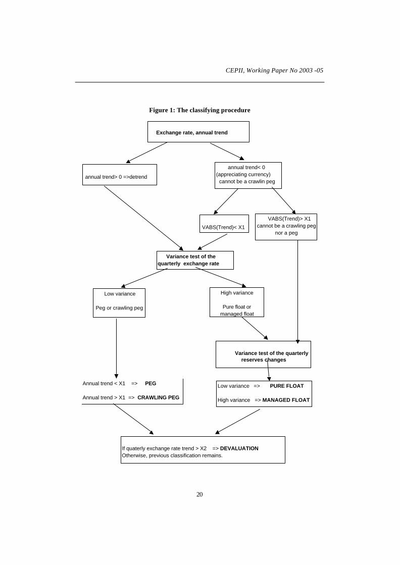
The method used to discriminate between these different regimes is based on a successionof tests (Figure 1). It can be compared to the technique used by Lambert and alii (2002) intheir empirical study of Latin American countries. In order to get round the problem ofwhat anchor to use, we assume the dollar to be the anchor currency in the sample, whichcomprises ten south-east Asian countries. This assumption is supported by studies onanchor currencies by Bénassy-Quéré (1996) and Bénassy-Quéré and Coeuré (2000).
We solve the problem of determining what constitutes high and low variance byconsidering there is a group of floating currencies – USD/DEM, USD/JPY and USD/GBP –which by definition have high exchange rate volatility and low reserve volatility. In this,we are drawing on an idea formulated by Calvo and Reinhart (2002). However, weimprove on their method by conducting formal statistical tests on the variances relatively tothis benchmark sample of floating currencies. We address the issue of unreliability ofannual classifications by drawing up a quarterly classification.
3.2 Sample and data
The study spans the 1990:1-2001:4 period and covers ten Asian countries: China, SouthKorea, Hong Kong, India, Indonesia, Malaysia, Pakistan, the Philippines, Singapore andThailand. The benchmark sample of floating currencies is made up of three countries:Germany (whose currency is the deutsche mark up to 1998 and the euro after 1999), Japanand the UK. As the classification is made on quarterly basis, an “observation” designates agiven quarter for a given country.
In order to construct quarterly variances, we use weekly exchange rates against dollar,extracted from the Datastream base and monthly data on official reserves from the IMF’sInternational Financial Statistics (see appendix 1).
All exchange rate series are taken as logarithm. The exchange rate is defined by thenumber of national currency units against the dollar, thus a positive change indicates adepreciating currency.

CEPII, Working Paper No 2003 -05
16
3.3 The classification process
Stage one: sorting observations by the annual trend in the exchange rate
The first stage consists in calculating annual trends from all the weekly exchange rate on acalendar-year basis. This stage is aimed at detecting crawling pegs. As crawling pegs aredesigned to pre-announce authorised devaluation rates, we separate the period of positivetrends, which correspond to a depreciating currency, from the period of negative trends. Asimplementations of crawling pegs are usually made at the beginning of a calendar year, wecompute trend on a calendar year basis.
§ If the trend is positive, we compute detrended series to distinguish betweenfixed regimes (pegs and crawling pegs) and floating regimes (pure ormanaged). Subsequently, the exchange rate series that we use are detrendedover periods where the trend is positive. We then go on to step two.
§ If the trend is negative, we have to establish whether it is “significant” or not.
A trend that is statistically significantly different from zero is not a sufficient criterion:if the trend is very small, we could not rule out the possibility that this might be apegged exchange rate oscillating weakly within fluctuation bands. For example whentrying to implement this method for Argentina during the period of currency board, wefound a significant trend for some years, although the rate of change was so small, thatthe exchange rate was clearly pegged. This kind of problem was also encountered byLevy-Yeyati and Sturzenegger (2000, 2003), who were not able to classify Argentinawithout setting an arbitrary threshold (in their case, the threshold was set onvolatilities).
So we assume a given threshold that we arbitrarily set at x1= 2% annually. This issimilar to the level adopted by Bubula and Ötker-Robe (2002). This threshold fits theallowed change in the exchange rate of a pegged currency with fluctuation margins of± 1%. This is the size of fluctuation band retained by the IMF for his definition of apegged exchange rate.
- If the negative trend has an absolute value smaller than x1, we go on to stage2 to determine whether we are dealing with a fixed exchange rate regime or afloat without trend.
- If the negative trend has an absolute value greater than x1 , the regime cannotbe a peg or a crawling peg. We therefore immediately deem the country tooperate a pure or a managed float, and go directly to stage four.
Stage two: Separating peg and crawling peg from float and managed float by comparingquarterly variances in the exchange rate with those of the benchmark sample.
We calculate quarterly variances in the exchange rate by using weekly data (detrended ifthe trend is found positive in stage one)). We compare the variances obtained for the Asian

Does Exchange Rate Regime Explain Differences in Economic Results for Asian Countries ?
17
economies to the average of the variances obtained for major benchmark floatingcurrencies.
Let us designate by 21S this empirical quarterly variance of the exchange rate for the Asian
country and by 20S the empirical quarterly variance of the reference sample. We assume
that exchange rates follow a normal distribution, with a theoretical variance ²1σ for the
Asian country and ²0σ for the benchmark sample. Therefore, the empirical variances,
21S , calculated with n1 observations, (n1=13 weekly observations in a quarter), follows a
chi-square distribution with (n1-1=12) degrees of freedom. Since 20S is the mean of the
empirical variances of the three benchmark floating exchange rates, it is calculated on thebasis of n0=13x3 data ; it follows a chi-square with n0-1=38 degrees of freedom. Therefore,the ratio of the two empirical variances divided by their theoretical values follows a Fisherdistribution:
( )1,1²/
²/10
12
1
02
0 −−→ nnFS
S
σ
σ (1)
The null hypothesis H0 is that in a given quarter, the variance of the exchange rate in theAsian country is smaller than the one of the benchmark sample of floating exchange rates:
H0 : 20
212
1
20 1 σσ
σ
σ<⇔> (2)
We carry out this variance equality test at a significance level of α=5%. We accept the nullhypothesis if the ratio of the empirical variances is such that :
αfS
S>2
1
20 (3)
where αf is the (1-α) quantile of the repartition function of F(n0-1, n1-1). This is
equivalent to the condition:
20
21
1S
fS
α< (4)
This amounts to consider that the exchange rate variance is “low” if it is smaller than 41%of the variance of the benchmark floating currencies. If it is greater, we reject the nullhypothesis and consider the country as having a “high” variance of his exchange rate duringthe quarter.
On the basis of this test, we are able to draw up a first sorting. In a given quarter, a countryis classified as a peg or a crawling peg if the null hypothesis is accepted, which means thathis exchange rate variance is smaller than 41% of the one of the benchmark sample.Otherwise, the country is deemed to have adopted a float or a managed float.
CEPII, Working Paper No 2003 -05
18
Stage three: Separation of pegs from crawling pegs on the basis of their annual trend
Any country qualified as pegged or crawling peg under stage two is classified as having apeg if the annual trend of its exchange rate (determined in stage one) is lower than x1=2%,and a crawling peg otherwise.
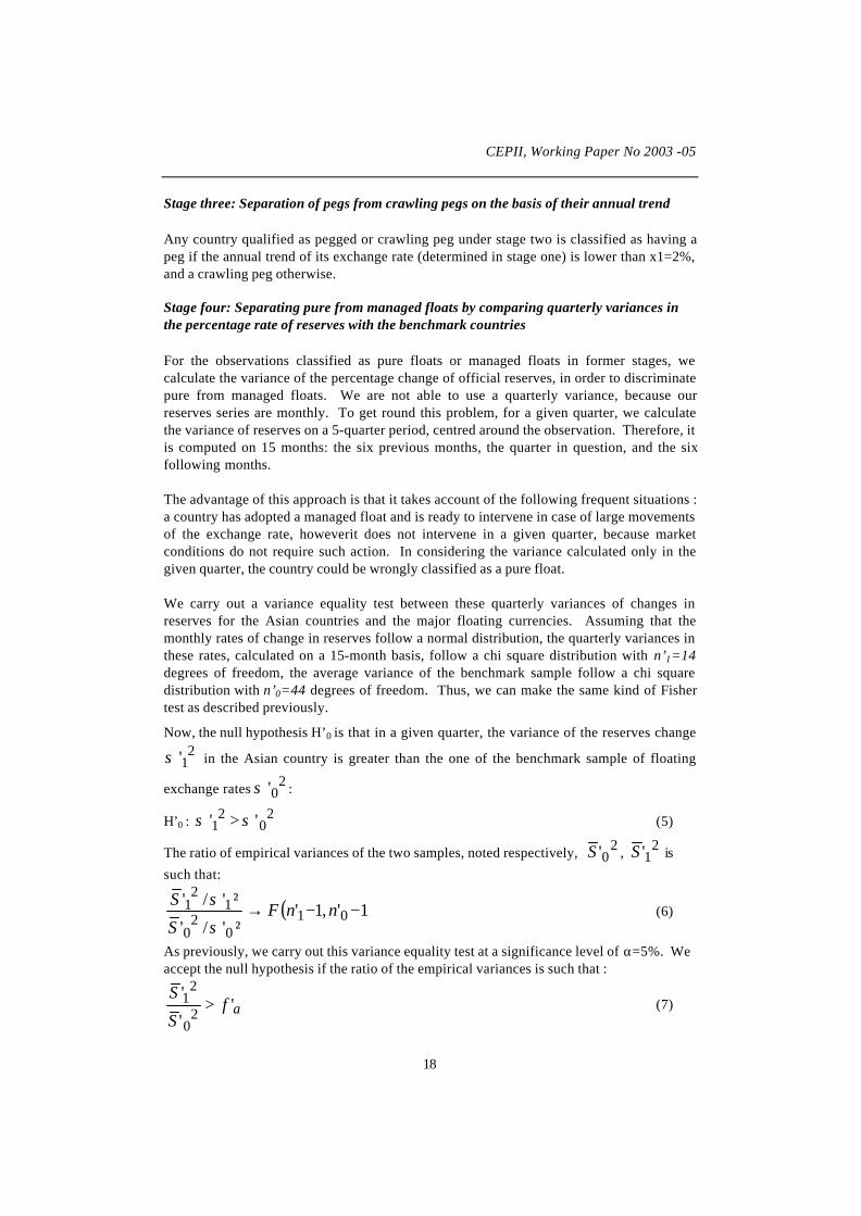
Stage four: Separating pure from managed floats by comparing quarterly variances inthe percentage rate of reserves with the benchmark countries
For the observations classified as pure floats or managed floats in former stages, wecalculate the variance of the percentage change of official reserves, in order to discriminatepure from managed floats. We are not able to use a quarterly variance, because ourreserves series are monthly. To get round this problem, for a given quarter, we calculatethe variance of reserves on a 5-quarter period, centred around the observation. Therefore, itis computed on 15 months: the six previous months, the quarter in question, and the sixfollowing months.
The advantage of this approach is that it takes account of the following frequent situations :a country has adopted a managed float and is ready to intervene in case of large movementsof the exchange rate, howeverit does not intervene in a given quarter, because marketconditions do not require such action. In considering the variance calculated only in thegiven quarter, the country could be wrongly classified as a pure float.
We carry out a variance equality test between these quarterly variances of changes inreserves for the Asian countries and the major floating currencies. Assuming that themonthly rates of change in reserves follow a normal distribution, the quarterly variances inthese rates, calculated on a 15-month basis, follow a chi square distribution with n’1=14degrees of freedom, the average variance of the benchmark sample follow a chi squaredistribution with n’0=44 degrees of freedom. Thus, we can make the same kind of Fishertest as described previously.
Now, the null hypothesis H’0 is that in a given quarter, the variance of the reserves change2
1'σ in the Asian country is greater than the one of the benchmark sample of floating
exchange rates 20'σ :
H’0 : 2
02
1 '' σσ > (5)
The ratio of empirical variances of the two samples, noted respectively, 20'S , 2
1'S is
such that:
( )1',1'²'/'
²'/'01
02
0
12
1 −−→ nnFS
S
σ
σ (6)
As previously, we carry out this variance equality test at a significance level of α=5%. Weaccept the null hypothesis if the ratio of the empirical variances is such that :
α''
'2
0
21 f
S
S> (7)

Does Exchange Rate Regime Explain Differences in Economic Results for Asian Countries ?
19
where α'f is the (1-α) quantile of the repartition function of F(n’1-1, n’0-1). This is
equivalent to the condition:
20
21 ''' SfS α> (8)
This amounts to considering that the regime is a managed float if the reserves changeshave a variance, which is greater than 2 times the variance of the benchmark sample. Ifnot, the observation is classified as a pure float.
Stage five: detecting devaluation
In a final and independent stage, we calculate quarterly deterministic trends for eachobservation in order to identify periods in which a devaluation has occurred. If thequarterly trend is greater than a given threshold x2, we classify the observation as adevaluation. Therefore, this category includes ruptures of pegs and crawling pegs, but alsosharp depreciation periods in floating and managed floats regimes.
Given our sample of Asian countries, where inflation is low and nominal depreciations aremoderate except during crises, we set the threshold at 6%. Obviously, this threshold,somewhat arbitrary, depends on the sample. It seems to fit to what we know of devaluationsize in the area. If we had been dealing with Latin America, for example, we would haveset a higher level. For European Union countries, for example in the former Exchange RateMechanism, this would have been smaller, as devaluation of 2 or 3% occurred.
CEPII, Working Paper No 2003 -05
20
Figure 1: The classifying procedure
Exchange rate, annual trend
annual trend< 0 (appreciating currency) cannot be a crawlin peg
VABS(Trend)< X1
VABS(Trend)> X1cannot be a crawling peg
nor a peg
Variance test of the quarterly exchange rate
Low variance
Peg or crawling peg
High variance
Pure float or managed float
Variance test of the quarterly
reserves changes
Annual trend < X1 => PEG
Annual trend > X1 => CRAWLING PEG
Low variance => PURE FLOAT
High variance => MANAGED FLOAT
If quaterly exchange rate trend > X2 => DEVALUATION Otherwise, previous classification remains.
annual trend> 0 =>detrend

Does Exchange Rate Regime Explain Differences in Economic Results for Asian Countries ?
21
4. CLASSIFICATION RESULTS
We used this method of successive tests to draw up a quarterly classification for exchangerate regimes adopted by the ten Asian countries under examination over the 1990-2001period. To facilitate comparison between the existing classifications, and to present theresults in a more condensed form, we draw an annual classification from the quarterlyfigures (table 4). The annual exchange rate regime presented in this table is the one foundin the majority of the four quarters. If two regimes share equal prominence, both areindicated. This annual classification is only provided for giving a synthetic view of theresults in this section. It is not used in the calculations performed in section 5. Completequarterly results are given in appendix 2.
4.1 de facto exchange rate policies of the Asian countries
This "de facto" classification highlights some stylised facts about the exchange rate policyin the area. It exhibits the strong links of the Asian currencies to the dollar until the 1997crisis and the softening of this constraint afterwards.
Table 4: De facto exchange rate regimes identified by our classification method
Thailand Malaysia India Indonesia HongKong
1990 Float Peg Crawl n.a Peg 1991 Peg Peg Managed/Devaluation n.a Peg 1992 Peg Float Craw l/Devaluation Crawl Peg 1993 Peg Peg Crawl/Devaluation Crawl Peg 1994 Peg Managed Peg Crawl Peg 1995 Peg Peg Crawl/Devaluation Crawl Peg 1996 Peg Peg Peg/Float Peg Peg 1997 Managed/Devaluation Managed/Devaluation Crawl/Devaluation Float/Devaluation Peg 1998 Float/Devaluation Float/Devaluation Crawl/Devaluation Float/Devaluation Peg 1999 Crawl/Devaluation Peg Crawl Float/Devaluation Peg 2000 Crawl Peg Crawl Float/Devaluation Peg 2001 Crawl/Float Peg Crawl Float/Devaluation Peg
China Philippines South Korea Singapore Pakistan 1990 n.a n.a Crawl Float Crawl 1991 n.a n.a Crawl Float Crawl 1992 Devaluation Float/Devaluation Crawl Peg Crawl 1993 Crawl/
Devaluation Crawl/Float Crawl Float Managed/Devaluation
1994 Managed/ Float
Managed/Float Float Float Peg
1995 Peg Crawl/Devaluation Peg Peg Crawl/Devaluation 1996 Peg Peg Crawl/Float Peg Managed/Devaluation 1997 Peg Managed/Devaluation Managed/Devaluation Crawl/Devaluation Crawl/Devaluation 1998 Peg Devaluation Managed/Devaluation Peg/Devaluation Managed/Devaluation 1999 Peg Crawl/Devaluation Peg Peg Crawl 2000 Peg Crawl/Float Crawl/Devaluation Crawl Crawl/Devaluation 2001 Peg Float Float Crawl Crawl/Managed

CEPII, Working Paper No 2003 -05
22
Between 1990 and 1995, six countries (Thailand, Indonesia, India, Korea, Hong Kong,Pakistan), among the ten in the sample, chose exchange rate regimes directly anchored tothe dollar (peg or crawling peg). The four other countries adopted a more flexible regime,without letting their currency freely float, except Singapore between 1993 and 1994.Broadly, this period is characterised by large interventions of the monetary authorities inorder to stabilise their currency. As suggested by the strong growth of reservesaccumulated over the period, the interventions mainly consisted in limiting the appreciationof the currencies relatively to the dollar, with the aim of maintaining competitiveness.
During this period, there was a general tendency to harden the peg: Thailand adopted a pegfrom the beginning of 1990, followed by China in 1994; other countries, like Singapore,hitherto in managed float, reduced their band of fluctuation de facto with respect to thedollar. In 1996, 8 countries out of the ten (Thailand, Malaysia, the Philippines, China,Indonesia, India, Singapore, Hong Kong) followed a strict peg anchored on the dollar.Only Pakistan and Korea preserved some flexibility of their exchange rate versus dollar.However, maintaining the peg was getting more and more difficult, in the countries, likeThailand, where financial liberalisation was implementing and international flows of capitalwere growing huge.
The outburst of the speculation at the time of the 1997-1998 crisis was lethal for the fixedregimes without capital controls (Thailand, Philippines, Indonesia, Malaysia), leading themonetary authorities to devaluate massively. China was able to maintain the peg becauseof rigorous exchange rate controls, and also because of a former devaluation in 1994.Hong-Kong was protected by large amounts of forex reserves and his particular politicalstatute. India and Pakistan kept out the crisis, because of their geographical remoteness andalso because they were protected by strict foreign exchange controls; they were able tocontinue their intermediate regimes, alternating periods of crawling pegs, devaluation, andmanaged float.
In the aftermath of the crisis, the concerned countries shifted to more flexible regimes: purefloat for Korea, Indonesia and Singapore, managed float for Thailand and the Philippines.This result is in line the findings by Hernandez and Montiel (2001). Malaysia was able tocome back to a pegged exchange rate, because of her decision to implement strict exchangerate controls, in spite of the disapproval of the IMF.
4.2 Comparison with other classifications
Table 5 shows how the countries in our sample are classified by LYS method. The LYSclassification has the advantage of spanning a longer period (1973-2000) and covering amuch larger number of countries (172). However, it involves several drawbacks.
First, the crisis periods (between 1996 and 1998 depending on the country) are classified asfloats, whereas most of the countries suffered major devaluations. Second, LYS resultsmakes no distinction between crawling pegs and managed floats, a problem that applies to alarge number of years and countries (22% of years are classified as Dirty float/Crawlingpeg in the sample). Third, “inconclusive” observations account for 6% of the total, notablyIndia in 1992 and 1999, Indonesia in 1994 and Pakistan in 1993; China is not covered.Fourth, some results seem more accurate in our classification: for example, LYS see a dirtyfloat or a crawling peg in Thailand in the early nineties, our detected peg in year 1991-1993

Does Exchange Rate Regime Explain Differences in Economic Results for Asian Countries ?
23
and 1995-96 seems a better assessment of the exchange rate policy adopted at that time.LYS classify India as having a floating or inconclusive exchange rate regime in thenineties, while we see mostly crawling pegs with devaluations, more in line with theevidence shown by graph 1.
By using quarterly observations, we are able to detect intra-year changes in the exchangerate regime, which is not done by the LYS method. Furthermore, we discriminate betweencrawling pegs and managed floats; and identify devaluation. We also are able to classifyregimes that fall into the “inconclusive” category under the LYS approach. Table 5: De facto exchange rate regimes identified by the LYS classification method
Thailand Malaysia India Indonesia Hong Kong 1990 Dirty/CP Fixed Dirty/CP Fixed Fixed 1991 Dirty/CP Dirty/CP Float Fixed Fixed 1992 Dirty/CP Dirty Inconclusive Fixed Fixed 1993 Dirty/CP Dirty Float Fixed Fixed 1994 Dirty/CP Fixed Inconclusive Inconclusive Fixed 1995 Dirty/CP Float Float Dirty/CP Fixed 1996 Inconclusive Dirty/CP Float Dirty/CP Fixed 1997 Dirty/CP Float Float Dirty/CP Fixed 1998 Dirty/CP Dirty/CP Float Dirty Fixed 1999 Float Fixed Inconclusive Dirty/CP Fixed 2000 Float Fixed Dirty/CP Dirty/CP Fixed 2001 n.a n.a n.a n.a Fixed
China Philippines South Korea Singapore Pakistan 1990 n.a Float Dirty Dirty Dirty/CP 1991 n.a Dirty/CP Fixed Dirty Float 1992 n.a Dirty Dirty/CP Dirty Dirty/CP 1993 n.a Fixed Dirty/CP Fixed Float 1994 n.a Float Fixed Dirty/CP Inconclusive 1995 n.a Float Dirty Dirty Float 1996 n.a Fixed Fixed Dirty/CP Float 1997 n.a Float Dirty/CP Float Float 1998 n.a Float Dirty/CP Float n.a 1999 n.a Float Fixed Fixed n.a 2000 n.a Float Fixed Fixed n.a 2001 n.a n.a n.a n.a n.a
Source: Levy-Yeyati and Sturzenegger (2003)
The IMF’s classification is published in the “Exchange Rate Arrangements” tables,included in various issues of the International Financial Statistics (IFS). It is based onmember states’ declarations and differs considerably from the de facto classifications(Table 6). The classifying method has been improved since 1999, to include morecategories and also to take into account “de facto” management of the exchange rate.However, here, we consider the broad categories available on the whole period.

CEPII, Working Paper No 2003 -05
24
Table 6: Exchange rate regimes, reported to the IMF
Thailand Malaysia India Indonesia Hong Kong 1990 Pegged Pegged Floating Intermediate Pegged 1991 Pegged Pegged Floating Intermediate Pegged 1992 Pegged Pegged Intermediate Intermediate Pegged 1993 Pegged Intermediate Floating Intermediate Pegged 1994 Pegged Intermediate Floating Intermediate Pegged 1995 Pegged Intermediate Floating Intermediate Pegged 1996 Intermediate Intermediate Floating Intermediate Pegged 1997 Intermediate Intermediate Floating Floating Pegged 1998 Floating Pegged Floating Floating Pegged 1999 Floating Pegged Floating Floating Pegged 2000 Floating Pegged Floating Floating Pegged 2001 Floating Pegged Floating Floating Pegged
China Philippines South Korea Singapore Pakistan 1990 Intermediate Floating Intermediate Intermediate Intermediate 1991 Intermediate Floating Intermediate Intermediate Intermediate 1992 Intermediate Floating Intermediate Intermediate Intermediate 1993 Intermediate Floating Intermediate Intermediate Intermediate 1994 Intermediate Floating Intermediate Intermediate Intermediate 1995 Intermediate Floating Intermediate Intermediate Intermediate 1996 Intermediate Floating Intermediate Intermediate Intermediate 1997 Intermediate Floating Floating Intermediate Intermediate 1998 Intermediate Floating Floating Intermediate Intermediate 1999 Intermediate Floating Floating Intermediate Intermediate 2000 Pegged Floating Floating Intermediate Intermediate 2001 Pegged Floating Floating Intermediate Intermediate Source: IMF, IFS.
As Levy-Yeyati and Sturzenegger (2003) point out, their classification and that of the IMFbear certain similarities. However, the IMF’s classification, which is based on memberstates’ announcements, tends to overestimate the number of pure floats. This discrepancyevidenced by Calvo and Reinhart (2002), can be ascribed to a “fear of floating”.Furthermore, the IMF classification, like the LYS one, fails to take account of devaluations.This is a major drawback when assessing the macroeconomic impact of exchange rateregime, since such breaks are usually followed by sizeable recessions, as we will see in thenext section.
Compared with the IMF classification, the results are fairly homogenous. Ourclassification subdivides “intermediate” regimes into crawling pegs and managed floats.Unsurprisingly, and as with the LYS method, we find more pegged systems than does theIMF. Thus, we are capturing situations where a de facto fixed exchange rate system is inplace, but a float has been reported to the IMF. Also, by systematically detecting episodesof devaluation, our method offers a significant advantage for analysing the impact of theseexchange rate regimes on macroeconomic performance. Table 7 compares the resultsobtained using the different approaches.

Does Exchange Rate Regime Explain Differences in Economic Results for Asian Countries ?
25
Table 7: Comparison of results obtained by the three classification methods in theAsian sample, 1990-2000
Float Intermediate Fixed Inconclusive Devaluation
IMF 30% 47% 23% - -
LYS 24% 37% 33% 6% -
Our classification (1) 15.2% 34.5% 39.6% - 10.6%
(1) calculated on the basis of the quarterly classification
Source: authors’ calculations.
Table 7 provides telling evidence of the “fear of floating” brought to light by Calvo andReinhart (2000). Far fewer floats are detected using the statistical approach than arereported to the IMF. We detect even fewer of them than the LYS approach does, becausewe take into account crawling pegs and devaluation. Our classification confirms the strongties linking the Asian currencies to the dollar – almost 65% of the regimes are pegs orcrawling pegs – which are often cited as one of the main causes behind the 1997-1998crisis.
4.3 Average performance by category
Having classified observations by de facto regime, we are able to calculate average growthand inflation performance for each category (see table 8). However, the small number offloating exchange rates obtained in the classification does not allow to yield robustconclusions about them. As GDP growth is only available on a yearly basis, we use theyearly classification of table 4, for calculating the average growth per currency regime
4.
For inflation, we use the quarterly classification given in appendix.
One striking result is the monotonous relationship found between exchange rate flexibilityand these macroeconomic variables. As the regime flexibility increases, average growth ishigher and inflation lower. Regimes based on pure floats appear to achieve the highestgrowth over the sample, with average rates of 8.4%, while pegs yield the best inflationaryperformances, with average inflation of 4.8% compared to 9.2% for floats. Intermediateregimes, crawling pegs and managed float achieve intermediate performances.
4 When two regimes are given for one year, we take the one which is also found in the previous year. When
it is the case for both, we take the one that is also found in the following year.

CEPII, Working Paper No 2003 -05
26
Table 8: Average annual GDP growth and inflation, by exchange rate regime
GDP growth Annual basis
Inflation Quarterly basis
Number of observations Annual/Quarterly
Peg 6.0% 4.8% 40/164
Crawl 6.5% 7.4% 21/106
Managed 6.0% 7.5% 2/37
Float 8.4% 9.2.% 9/63
Devaluation 2.2% 8.4% 32/44
Source : authors’ calculations from IFS, IMF data
Devaluation periods recorded the lowest growth rates and a high rate of inflation. The firstof these points is noteworthy. According to these results, far from providing an economicstimulus, devaluations seem to trigger recession. This may result from unhedged liabilitiescontracted by domestic agents. These negative consequences of devaluation explain the“fear of floating” highlighted by Calvo and Reinhart (2002). However, here, the resultsonly concerns the simultaneous link between devaluation and growth, it does not precludethat lagged or long term effects could be positive.
These results on the averages for the different categories are nevertheless questionable, forthey are subject to an assumption of ceteris paribus. To lift this assumption, we have tobring in other control variables by performing regressions.
5. ECONOMETRIC ANALYSIS
To determine the impact of the exchange rate regime on growth and inflation in the tensample countries, we perform several regressions on panel data for the 10 countries over the1990-2001 period. We measure the effect of the exchange rate regime on macroeconomicperformance by inserting dummy variables representing them in the regression, as didLevy-Yeyati and Sturzenegger (2000). This method is also used to assess the impact ofexchange rate regime on other variables, such as the degree of currency mismatch Arteta(2003), or the probability of crisis (Domaç and alii (2003).
The dummy variables of exchange rate regimes are directly deduced from the classification
and constructed in the following way. The dummy kqtiD ,, , represents the existence of an
exchange rate regime of type k (k= peg, crawling peg, managed float, float or devaluation)in country i for the year t and quarter q :
1,, =kqtiD , when the country i is classified in the regime k in year t and quarter q i=
1…10, t= 1990, 2001, q=1,..4, k=peg, crawling peg, managed float, float or devaluation(9)
0,, =kqtiD , otherwise (10)

Does Exchange Rate Regime Explain Differences in Economic Results for Asian Countries ?
27
In each regression, we use one of these regimes as the benchmark, so its dummy is takenout of the equation. The coefficients of the other dummy variables then measure the impactof a given regime relative to the benchmark.
5.1 Impact on growth
As GDP data are only available on an annual basis, the regression is made on a yearlybasis, using yearly dummy variables for exchange rate regimes. For keeping the highdegree of precision given by our quarterly classification, the yearly dummy variables foreach exchange rate regimes are constructed by averaging the quarterly dummies describedin (5) and (6).
∑=
=4
1,,, 4
1
q
kqti
kti DD (11)
This simply amounts to set the dummy ktiD , equal to the number of quarters when the
regime k has been implemented, divided by four.
4,n
D kti = , when the country i is classified in the regime k during n quarters of the year t,
40 ≤≤ n (12)
0, =ktiD , otherwise (13)
We also introduce in the regression control variables, which are supposed to act on long-term growth. These variables are based on endogenous growth models. They can be foundin empirical studies of long-term growth, such as those by Barro (1991), Barro-Lee (1994),Razin-Collins (1997) and Levy-Yeyati-Sturzenegger (2001b). They are public spending oneducation (EDU), the growth rate of the total population (POP), the degree of openness(OPEN), the investment rate (INVEST) and the initial level of GDP per capita (GDP),which is designed to stand for the catching-up process.
The expected effects of the control variables are as follows. Education spending (EDU)should have a positive impact on growth, since such expenditure is generally viewed as animprovement in human capital. The population growth (POP) and the investment rate(INVEST) should also have a positive impact, insofar as they help to increase the factors ofproduction. The likely effect of the openness variable (OPEN) is less clear-cut. However,given that most countries in our sample have based their development strategy on exports, apositive impact can be expected. The initial GDP per capita (GDP) variable should have anegative impact, if these countries do “catch up”.
The series on growth and investment rates, exports, imports and GDP are taken from theIMF’s International Financial Statistics database. The series for public educationspending, population and GDP in purchasing power parity (PPP) come from the WorldBank database (see the appendix for a description of all variables and sources). Theopenness ratio is calculated as the sum of exports and imports relative to GDP. The catch-up variable (GDP) used is the GDP in PPP per capita in 1990. We consider the EDU, POPand INVEST variables to be constant for each country over the entire period because they

CEPII, Working Paper No 2003 -05
28
are supposed to have only a long-term effect. They are fixed at their average value over theperiod and standardised with respect to the sample average.
As we do not expect short-term effect of exchange rate regime, the growth data aresmoothed annually to remove cyclical effects. To do this, the average annual growth rate iscalculated as the average of the growth rates recorded in the year in question, the previousyear and the following year. Indeed, if exchange rate regimes affect economic growth, theeffects will involve mechanisms, such as the credibility effect, that could reduce interestrate in the case of pegged exchange rate or better softening of business cycle, that couldstabilise investment, for floating exchange rates. These effects will not be seenimmediately. That is why we also introduce a lag of one year on all the explanatoryvariables. The managed float regime is used as the benchmark. The coefficients of theother regimes’ dummy variables therefore measure the growth differential relative to themanaged float.
The regression on Table 9 measures the impact of the different regimes on growth with aone-year lag. The control variables are significant, except the investment rate, which isremoved from the regression. They all have their expected effect, except population.
According to these findings, episodes of fixed exchange rates generated markedly lowergrowth rates than did managed floats. In fact, pegs led to a 2.5% reduction in growth. Thisdifferential is significantly different from zero at a 10% level of significance. By contrast,growth under crawling peg and floating regimes was not different from that of managedfloats. Their coefficients are not significantly different from zero. Devaluations have themost harmful effects on growth. The growth rate during such periods is 11.8% lower thanthat recorded under managed floats. This coefficient is significantly different from zero at a1% level of significance.
These findings are consistent with the results of the average by exchange rate regime, madein the previous section, and also with those of Levy Yeyati and Sturzenegger(2001), thatevidenced a weaker growth for fixed exchange rate regimes. Ghosh, Gulde, Ostry andWolf (1997) also found a smaller growth for pegged exchange rate countries but their resultwas not significant. The findings on negative effects of devaluation on growth could beexplained by the severity of the exchange rate crises in the sample. It is also consistentwith the “fear of floating” evidenced by Calvo and Reinhart. As devaluation does not“pay”, emerging countries have better to maintain their exchange rate.

Does Exchange Rate Regime Explain Differences in Economic Results for Asian Countries ?
29
Table 9: GDP growth regression
Dependent variable: GDP growth
Method: Pooled Least Squares; Total panel observations 100
Variable Coefficient Std. Error t-Statistic Prob.
Constant 0.415 0.082 5.01 0.0000
Dummy PEG (-1) -0.025 0.014 -1.772 0.079
Dummy CRAWL (-1) 0.007 0.014 0.50 0.614Dummy FLOAT (-1) -0.00004 0.016 -0.149 0.9978
Dummy DEVALUATION (-1) -0.118 0.027 -4.38 0.0000
OPEN 0.045 0.012 3.56 0.0005
GDP -0.0419 0.010 -4.05 0.0001
EDU 0.027 0.012 2.19 0.0309
POP -0.071 0.0168 -4.21 0.0000
R-squared 0.352 Mean dependent variable 0.051
Adjusted R-squared 0.295 S.D. dependent variable 0.042
S.E. of regression 0.035 Sum squared residuals 0.114
F-statistic 6.187 Durbin-Watson statistic 0.936
Prob (F-statistic) 0.000000
5.2 Endogeneity and growth
It is possible to have a two-way causality between economic performance and the exchangerate regime. In other words, macroeconomic performance may be a function of theexchange rate regime, which is what we are testing here, but the reverse may also be true,i.e. economic conditions themselves may drive certain choices of exchange rate regimes.We only partly address this problem of uncertain causality in the previous section byintroducing a lag of one year in the dummy variables in the regressions. Here, weinvestigate further this issue.
What would the reverse causality mean? This would imply that the monetary authoritieschoose the exchange rate regime according to the growth rate. This hypothesis is notjustified by the economic literature on the subject. The empirical studies by Edwards(1996), Rizzo (1998), Poirson (2001), Juhn and Mauro (2002) and Bénassy-Quéré andCoeuré (2002) do not retain growth among the determinants of exchange rate regime. Thisvariable is not present in the 14 studies on the subject reviewed by Juhn and Mauro (2002).Only the level of GDP is tested, for example by Edwards (1996), Rizzo (1998), Poirson(2001), Juhn and Mauro (2002) and also Alesina and Wagner (2003), in order to accountfor the size of the country; and also, the GDP per capita, standing for the level ofdevelopment, which is anyway quite a different variable from the GDP growth.

CEPII, Working Paper No 2003 -05
30
Nevertheless, we use the procedure of White (1984), which allows to address the problemof possible endogeneity of the exchange rate dummies and at the same time to correctproblems of heteroscedasticity. This method consists in using an instrumental variableregression in order to obtain an estimated occurrence probability of each exchange rateregime.
In a first step, we make a multilogit, regressing the exchange rate dummies on explanatoryinstrumental variables. The explanatory variables are those supposed to explain thecountries’ exchange rate regime choice in the studies mentioned above. They are also takenfrom Levy-Yeyati and Sturzenegger (2001) and Arteta (2003), that tried to address thequestion of endogeneity on the same type of equations. Here, we retain the followingvariables: the openness ratio; the investment rate; the ratio of domestic credit to GDP; theratio of quasi-money to money – these two latter variables measure the financial depth ofthe economy - and the ratio of initial reserves to GDP, which measures the capacity of thecentral bank to defend a fixed exchange rate. These variables are taken annually. Theregression enables us to obtain the estimated probabilities of each regime, according to thecharacteristics of the country. In the second step, we make a new regression on growthwhere regime dummies are replaced by the estimated values of their probabilities.
Results, presented in table 10, confirm those of the first regression (table 9). Growthperformances remain more limited for anchored than for floating regimes. As previously,pure floats do not seem to have generated significant differences in growth compared tomanaged floats. The only difference between the two regressions concerns crawling pegs,that seem here to have yield a lower growth than managed floats. For this secondregression, the interpretation of the coefficients associated with each regime is notstraightforward, since the dummies are now probabilities, always smaller than unity.

Does Exchange Rate Regime Explain Differences in Economic Results for Asian Countries ?
31
Table 10: Comparative regressions on growth of GDP
Dependent variable:GDP growth
Initial regressionPooled Least Squares
Two-step regression withinstrumental variables for dummies
0.415*** 0.409***Constant(5.01) (4.29)
-0.025* -0.210**Dummy PEG (–1)(-1.77) (-2.38)
0.007 -0.355***Dummy CRAWL(-1)(0.50) (-2.97)
-0.00004 -0.0815Dummy FLOT(-1)(-0.0023) (-0.779)
-0.118*** -0.029***Dummy DEV(-1)(-4.38) (-3.64)
-0.071*** -0.058***POP(-4.21) (-3.04)
-0.041*** -0.026**GDP(-4.05) (-2.18)
0.045*** 0.030OPEN(3.56) (1.25)
0.027** 0.044**EDU(2.19) (2.45)
Results of the instrumental variables regression
R-squared 0.430 Mean dependent variable 0.051
Adjusted R-squared 0.380 S.D. dependent variable 0.042
S.E. of regression 0.0335 Sum squared residuals 0.101
F-statistic 8.5021 Durbin-Watson statistic 0.916
Prob (F-statistic) 0.0000 Panel observations 99
Note :***, ** * stand for coefficients respectively 99%, 95% and 90% percent significantly differnetfrom zero. Figures in brackets are t-statistics.
5.3 Impact on inflation
Because inflation is more reactive than growth, we employ quarterly data to measure theimpact of exchange rate regimes on inflation. Therefore, we use the quarterly dummyvariables described in equations (9) and (10).
We start from the following model, where the inflation rate π is a function of thelogarithmic change in the money supply ∆m, the growth in GDP ∆GDP and the interest rater :
π = a∆m + ß∆GDP +γ r (14)

CEPII, Working Paper No 2003 -05
32
We add to this equation the dummy variables for the exchange rate regimes. As growth isnot available on a quarterly basis, it is the same smoothed annual variable, as previouslyreplicated for each quarter.
The variables are expected to have the following effects. Changes in the money supplyshould have a positive impact on inflation (a positive), given that any increase in the moneysupply is likely to result in a price rise. GDP growth should have a positive impact (ßpositive), via a Phillips curve, assuming that high growth rates are likely to cause economicactivity to heat up and wages and prices to rise. The impact of interest rates is harder topredict. In theory, a negative sign might be expected, since high interest rates signal a tightmonetary policy that is likely to curb inflation by slowing activity and lowering investment.However, a reverse causal link is possible, through the central banks’ reaction function,which responds to high inflation rates by hiking interest rates. This would also beconsistent with a “Fisher” effect.
The data on inflation, changes in the money supply and interest rates are taken from theIMF’s quarterly IFS database. We introduce a one-year lag for the peg dummy variableand a six-month lag for devaluations. Price inertia supplies the justification for these lags.Moreover, a peg is unlikely to cause inflation to abate immediately; rather the impact willbe felt after a delay, through a decline in expected inflation as the peg gains in credibility.As for the growth regression, we use the managed float as the benchmark regime for thisregression.
The regression on Table 11 measures the impact on inflation of different exchange ratearrangements. The control variables do have the expected effect. The findings demonstratethat fixed regimes were followed by lower inflation Pegs generated 1.5% lower inflationthan managed float. This difference is significantly different from zero. On the contrary,pure floats were associated by an increase in inflation, estimated at 1.7%. By contrast,crawling pegs showed no difference from a managed float in terms of inflation, as itscoefficient was not significant. As expected, devaluations were followed by an upturn ininflation, which was 2.1% higher than that recorded by managed floats.
These results on inflation are consistent with the conclusions of Levy Yeyati andSturzenegger (2001) and of Ghosh, Gulde, Ostry and Wolf (1997). However, Levy Yeyatiand Sturzenegger(2001) made a distinction between "long peg” and "short peg" whileshowing the under-performance associated with "short peg" regimes. This latter categorycorresponds to the fixed exchange rates with frequent adjustments of parity in Ghosh andalii (1997). Here, we proceed by separating the periods of rupture of pegs and we identifythem with the “devaluation” dummy. We find that pegs are associated with lower inflation,while devaluation has a large inflationary effect. Concerning pure floats, our resultsconfirm those of Levy Yeyati and Sturzenegger (2001b) and of Ghosh and alii (1997), byshowing that they are significantly more inflationary.

Does Exchange Rate Regime Explain Differences in Economic Results for Asian Countries ?
33
Table 11: Inflation regression
Dependent variable: inflation rate
Method: Pooled Least Squares
Total panel observations 358 , sample(adjusted): 1991:1 2000:4Variable Coefficient Std. Error t-statistic Prob.
Constant -7.14 1.27 -5.62 0.0000
Dummy PEG(-4) -1.468 0.71 -2.04 0.0411Dummy CRAWL 0.330 0.78 0.42 0.6747
Dummy FLOAT 1.70 0.91 1.87 0.0622
Dummy DEVALUATION(-2) 2.123 1.06 2.00 0.046
GDP growth 0.137 0.07 1.97 0.0048
Money growth? 0.075 0.03 2.67 0.0078
Interest rate 1.021 0.07 13.6 0.0000
R-squared 0.48 Mean dependent variable 6.78
Adjusted R-squared 0.47 S.D. dependent variable 8.077
S.E. of regression 5.87 Sum squared residuals 12065.08
Log likelihood -817.34 F-statistic 46.51
Durbin-Watson statistic 0.354 Prob(F-statistic) 0.00000
The findings of these regressions confirm the analysis of the previous section. In otherwords, fixed exchange rate regimes generated lower inflation, but at the price of weakergrowth. Floating regimes had higher inflation, but not stronger growth. Overall, theintermediate regimes – managed floats and crawling pegs – appeared to achieve goodresults in terms of growth and inflation.
5.4 Inflation and endogeneity
We also try to address the issue of endogeneity of the exchange rate regime to inflation. Areverse causality in the inflation regression is more likely than for growth, as inflation mayplay a role in the choice of an exchange rate regime. Two effects are possible.
First, a country could choose a fixed exchange rate because he already has a low inflation.This makes the peg more sustainable, since it avoids the main drawback of pegs, which isthe real exchange rate appreciation and subsequent loss of competitiveness. Poirson (2001)found this kind of effect in her cross-section regression on 93 countries for year 1999: thehigher the inflation rate, the more likely is the adoption of a flexible regime. This sign wasalso found by Edwards (1996) and Rizzo (1998).
Second, the reverse mechanism could be true. A country could adopt a peg because of hishigh inflation, if he expects that the peg could bring more discipline and credibility to thegovernment policy. This was clearly the case of countries like Argentina, Estonia,
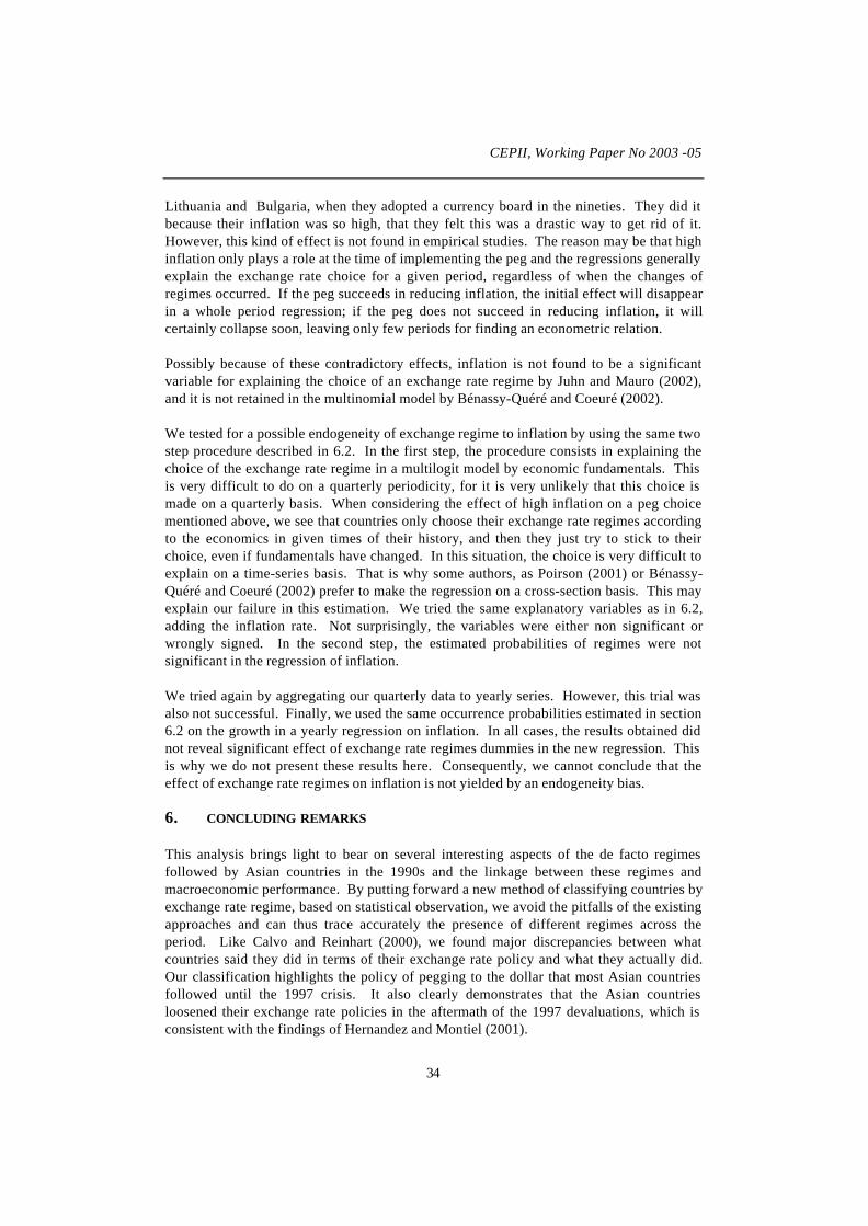
CEPII, Working Paper No 2003 -05
34
Lithuania and Bulgaria, when they adopted a currency board in the nineties. They did itbecause their inflation was so high, that they felt this was a drastic way to get rid of it.However, this kind of effect is not found in empirical studies. The reason may be that highinflation only plays a role at the time of implementing the peg and the regressions generallyexplain the exchange rate choice for a given period, regardless of when the changes ofregimes occurred. If the peg succeeds in reducing inflation, the initial effect will disappearin a whole period regression; if the peg does not succeed in reducing inflation, it willcertainly collapse soon, leaving only few periods for finding an econometric relation.
Possibly because of these contradictory effects, inflation is not found to be a significantvariable for explaining the choice of an exchange rate regime by Juhn and Mauro (2002),and it is not retained in the multinomial model by Bénassy-Quéré and Coeuré (2002).
We tested for a possible endogeneity of exchange regime to inflation by using the same twostep procedure described in 6.2. In the first step, the procedure consists in explaining thechoice of the exchange rate regime in a multilogit model by economic fundamentals. Thisis very difficult to do on a quarterly periodicity, for it is very unlikely that this choice ismade on a quarterly basis. When considering the effect of high inflation on a peg choicementioned above, we see that countries only choose their exchange rate regimes accordingto the economics in given times of their history, and then they just try to stick to theirchoice, even if fundamentals have changed. In this situation, the choice is very difficult toexplain on a time-series basis. That is why some authors, as Poirson (2001) or Bénassy-Quéré and Coeuré (2002) prefer to make the regression on a cross-section basis. This mayexplain our failure in this estimation. We tried the same explanatory variables as in 6.2,adding the inflation rate. Not surprisingly, the variables were either non significant orwrongly signed. In the second step, the estimated probabilities of regimes were notsignificant in the regression of inflation.
We tried again by aggregating our quarterly data to yearly series. However, this trial wasalso not successful. Finally, we used the same occurrence probabilities estimated in section6.2 on the growth in a yearly regression on inflation. In all cases, the results obtained didnot reveal significant effect of exchange rate regimes dummies in the new regression. Thisis why we do not present these results here. Consequently, we cannot conclude that theeffect of exchange rate regimes on inflation is not yielded by an endogeneity bias.
6. CONCLUDING REMARKS
This analysis brings light to bear on several interesting aspects of the de facto regimesfollowed by Asian countries in the 1990s and the linkage between these regimes andmacroeconomic performance. By putting forward a new method of classifying countries byexchange rate regime, based on statistical observation, we avoid the pitfalls of the existingapproaches and can thus trace accurately the presence of different regimes across theperiod. Like Calvo and Reinhart (2000), we found major discrepancies between whatcountries said they did in terms of their exchange rate policy and what they actually did.Our classification highlights the policy of pegging to the dollar that most Asian countriesfollowed until the 1997 crisis. It also clearly demonstrates that the Asian countriesloosened their exchange rate policies in the aftermath of the 1997 devaluations, which isconsistent with the findings of Hernandez and Montiel (2001).

Does Exchange Rate Regime Explain Differences in Economic Results for Asian Countries ?
35
The econometric results show that fixed exchange rate regimes are associated to betterperformances in terms of inflation. This confirms those of previous studies, as those ofLevy Yeyati and Sturzenegger (2001) and of Ghosh and alii (1997). This result seems toappear here more clearly because, thanks to a quarterly classification, we are able toseparate the periods of peg - which are associated with low inflation – from the ruptures ofanchoring, which generally correspond to devaluations generating a strong inflationaryeffect. Nevertheless, we cannot exclude the hypothesis that this result is due to anendogeneity bias, by which countries with low inflation are more likely to choose a peggedexchange rate. The regressions also show that pegs dampened GDP growth, compared tomanaged floats. This result is shown to persist after correcting for endogeneity.Furthermore, pegs are sometimes followed by severe devaluation, which causes growth tocollapse, in the concerned countries.
Floating regimes are shown to be linked to higher inflation, but fail to generate highergrowth than intermediate systems. Therefore, intermediate regimes – the managed floatand the crawling peg –appear to be reasonable options: they yield the highest GDP growthand are associated with intermediate results in terms of inflation. These results areconsistent with those of Williamson (2000), who found that intermediate arrangementswere the most suitable for emerging economies.
CEPII, Working Paper No 2003 -05
36
BIBLIOGRAPHY
Alesina, A. and A. Wagner (2003), “Choosing (and reneging) exchange rate regimes”,NBER Working paper 9809.
Arteta, C. (2003), “ Exchange rate regimes and financial dollarization: Does flexibilityreduce currency mismatches in bank intermediation? ”, Board of Governors of theFederal Reserve System, International Finance Discussion Papers n° 738.
Auernheimer, L. and S. Georges (2000), “Bad dreams under alternative anchors; are theconsequences different?”, IMF Working Paper WP/00/120.
Barro, R. (1991), “Economic Growth in a Cross-Section of Countries”, Quarterly Journal ofEconomics 16, p 406-443.
Barro, R. and J. Wa Lee (1994), “Sources of Economic Growth”, Carnegie-RochesterConference Series on Public Policy 40, p1-46.
Bénassy-Quéré, A. (1996), “Régimes et politiques de change en Asie”, EconomieInternationale no. 66.
Bénassy-Quéré, A. and B. Coeuré (2000), “Big and small currencies: the regionalconnection”, Document de travail CEPII n°2000-10.
Bénassy-Quéré, A. and B. Coeuré (2002), “ The survival of intermediate exchange rateregimes ”, CEPII, Document de travail 2002-07.
Bénassy-Quéré, A. and B. Coeuré (2003), “ On the identification of de facto currencypegs ”, mimeo.
Bordo, M., Eichengreen, B., Klingebiel, D. and Martinez Peria, M.S. (2001), “ Is the crisisproblem growing more severe? ”, Economic Policy 31, 51–82.
Bubula, A. and I. Ötker-Robe (2002), “The evolution of exchange rate regimes since 1990:evidence from de facto pegs”, IMF Working Paper WP/2002/155.
Calvo, G. and C. Reinhart (2000), “ Fixing for your life. ”, NBER, Working Paper No.8006.
Calvo, G. and and C. Reinhart (2002), “ Fear of floating ”, Quarterly Journal of Economics117, pp. 379–408.
Calvo, G. and F. Mishkin (2003), “ The mirage of exchange rate regimes for emergingcountries ”, NBER, Working Paper No. 9808.
Coudert, V. (2004), “Exchange rate Regimes and Crises: are Fixed Exchange Rates Reallyto Blame?, ” Working Paper CEPN, forthcoming, University of Paris 13,http://www.univ-paris13.fr/cepn.htm, also available in French : « Régimes de changeet crises: Les taux de change fixes sont-ils injustement suspectés?”, in R. Boyer, M.
Does Exchange Rate Regime Explain Differences in Economic Results for Asian Countries ?
37
Dehove and D. Plihon : “Les crises financières, analyses et propositions”, rapport duConseil d’Analyse Economique, à paraître, juillet 2004.
Domaç, I. and M. Soledad Martinez Peria (2003), “ Banking crises and exchange rateregimes: is there a link? ”, Journal of International Economics 61, pp. 41–72.
Dornbusch, R. (2001), “ Fewer monies, better monies ”, NBER,Working paper No. 8324.
Edwards, S. (1996), “The determinants of the choice between fixed and flexibleexchange-rate regimes,” NBER Working Paper, No. 5756.
Eichengreen, B. and P. Masson Paul (2000), “Exit strategies: Policy options for countriesseeking greater exchange rate flexibility”, IMF Occasional Paper, no. 168.
Fischer, S. (2001), “Exchange rate regimes: is the bipolar view correct?”, Lecture onEconomics in Government, American Economic Association Meeting, New Orleans.
Frankel, J.A. and Wei S.J. (1993), “Trade Blocs and Currency Blocs”, in NBER WorkingPaper no. 4335.
Frankel, J., S. Schmukler and L. Serven (2000), “Verifiability and the vanishingintermediate exchange rate regime”, NBER Working Paper No. 4901.
Frankel, J. (1999), “No single currency regime is right for all countries or at all times”,NBER Working Paper No. 7338.
Ghosh A., A.-M. Gulde, J. Ostry and H. Wolf (1997), “ Does the nominal exchange rateregime matter? ”, NBER, Working Paper 5874.
Hausmann, R., M. Gavin, C. Pages-Serra and E. Stein (1999), “ Financial Turmoil and theChoice of Exchange rate regime ”, Inter-American Development Bank, WORKINGPAPER n°400.
Hernandez, L. and P.J. Montiel P.J. (2001), “Post-crisis exchange rate policy in five Asiancountries: filling in the ‘hollow middle’, mimeo.
Juhn, G. and P. Mauro (2002), “Long-Run Determinants of Exchange Rate Regimes: ASimple Sensitivity Analysis”, IMF Working Paper WP/02/104.
Lahiri, A. and C. Végh (2001), “Living with the Fear of Floating: An Optimal PolicyPerspective”, NBER Working Paper No..
Lambert, F., C. Rebillard and J. Vierling (2002), “Quel régime de change pour les paysémergents, étude empirique sur les pays d’Amérique latine”, mimeo, ENSAE workinggroup steered by V. Coudert.
Levy Yeyati, E. and F. Sturzenegger (2000), “ Classifying Exchange rate regimes: Deedsversus Words ”, mimeo, Universidad Torcuato di Tella, forthcoming in EuropeanEconomic Review.

CEPII, Working Paper No 2003 -05
38
Levy Yeyati, E. and F. Sturzenegger (2001), “ Exchange Rate Regimes and EconomicPerformance ”, IMF, Staff papers, vol 47.
Levy Yeyati E. and F. Sturzenegger (2003), “A de facto Classification of Exchange RateRegimes: A Methodological Note,” American Economic Review, Vol. 93, No. 4.
Masson, P. (2000), “Exchange rate regime transitions” Journal of Development Economics,Vol 64, pp 571-586.
Obsfeld, M. and K. Rogoff, (1995), “ The mirage of fixed exchange rates ”, NBERWorking Paper No. 5191.
Miotti, L. D. Plihon and C. Quenan (2001), “The euro and financial relations between LatinAmerica and Europe: medium- and long-term implications”, mimeo, CEPAL, UnitedNations.
Poirson, H. (2001), “How do countries choose their exchange rate regime?”, IMF WorkingPaper WP/01/46.
Popper, H. and J. Lowell (1994), "Officially Floating, Implicitly Targeted Exchange Rates:Examples from the Pacific Basin" in R. Glick and M. Hutchison, eds., Exchange RatePolicy and Interdependence: Perspectives from the Pacific Basin, CambridgeUniversity Press.
Razin, O. and S. Collins (1997), “Real exchange rate misalignment and growth”, NBERWorking Paper No. 6174.
Reinhart, C. (2000), “The mirage of floating exchange rates”, American Economic Review,May 2000.
Reinhart, C. and K. Rogoff (2002), “The Modern History of Exchange Rate Arrangements:A Reinterpretation”, NBER Working Paper 8963, June 2002, forthcoming inQuarterly Journal of Economics.
Rizzo, J.-M. (1998), “The economic determinants of the choice of an exchange rate regime:a probit analysis,” Economics Letters, 59, No. 3, 283–287.
Rogoff, K., A. Husain and A. Mody, R. Brooks, N. Oomes (2003), “ Evolution andPerformance of Exchange Rate Regimes ”, IMF Working Paper, WP/2003/243.
Von Hagen, J. and J. Zhou (2004), The Choice of Exchange Rate Regime in DevelopingCountries: A Multinational Panel Analysis CEPR Discussion Paper No. 4227
White, H. (1984), Asymptotic Theory for Econometricians, Academic Press, New York.
Wickam, P. (2002), “Do flexible exchange rates of developing countries behave like thefloating exchange rates of industrialized countries?”, IMF Working Paper.

Does Exchange Rate Regime Explain Differences in Economic Results for Asian Countries ?
39
Williamson, J. (2000), “ Exchange Rate Regimes for Emerging Markets Reviving theIntermediate Option ”, Institute for International Economics, Policy Analyses inInternational Economics 60.

CEPII, Working Paper No 2003 -05
40
Appendix 1
Classification of de facto exchange rate regimes:
Sample period: 1990-2001.
Countries: China, South Korea, Hong Kong, India, Indonesia, Malaysia, Pakistan,Philippines, Singapore and Thailand.
Benchmark sample for the floating regime: Germany, UK and Japan.
Exchange rate series: weekly series taken from the Datastream base.
Reserves: series taken from the IFS base (1LDZF series)
Growth regression:
Dependent variable: GDP growth rate at constant prices calculated as the change in realGDP at constant 1995 prices. Source: IFS (99BVPZF series).
Control variables:
• Education spending (DPE): average ratio of education spending to GDP over theperiod, standardised with respect to the sample average. Source: World Bank.
• Total population (POP): average growth rate of the total population over theperiod, standardised with respect to the sample average. Source: World Bank.
• Investment (INVEST): average ratio of GFCF to GDP over the period,standardised with respect to the sample average. Source: IFS (99BZF and 93EZFseries).
• Openness (OP): average ratio of the sum of imports and exports to GDP over theperiod. Source: IFS (70ZF, 71ZF and 99BZF series).
• Catch-up (GDP): GDP PPP per capita in 1990 for each country considered.Source: World Bank.
Inflation regression:
Dependent variable: inflation, measured by the growth rate of consumer prices. Source: IFS(64ZF series).
Control variables:
• GDP growth rate at constant prices: change in real GDP at constant 1995 prices.Source: IFS (99BVPZF series).
• Change in the money supply. Source: IFS (34XZF series).• Interest rate. Source: IFS (60PZF series).


CEPII, Working Paper No 2003 -05
4
Appendix 2: Results of the classification of de facto exchange rate regimes
Thailand Malaysia Philippines China Indonesia India Korea Singapore Hong Kong Pakistan
1990:1 Float Peg N/A N/A N/A Crawl Crawl Float Peg Crawl
1990:2 Float Peg N/A N/A N/A Crawl Crawl Float Peg Crawl
1990:3 Float Peg N/A N/A N/A Crawl Crawl Float Peg Crawl
1990:4 Float Peg N/A N/A N/A Crawl Crawl Float Peg Crawl
1991:1 Peg Peg N/A N/A N/A Devaluation Crawl Float Peg Crawl
1991:2 Peg Peg N/A N/A N/A Devaluation Crawl Float Peg Crawl
1991:3 Peg Peg N/A N/A N/A Managed Crawl Float Peg Crawl
1991:4 Peg Peg N/A N/A N/A Managed Crawl Float Peg Crawl
1992:1 Peg Float Float N/A Crawl Devaluation Crawl Peg Peg Crawl
1992:2 Peg Float Devaluation Devaluation Crawl Crawl Crawl Peg Peg Crawl
1992:3 Peg Float Float N/A Crawl Crawl Crawl Peg Peg Crawl
1992:4 Peg Float Float Devaluation Crawl Crawl Crawl Peg Peg Crawl
1993:1 Peg Peg Crawl Devaluation Crawl Devaluation Crawl Float Peg Crawl
1993:2 Peg Peg Float Crawl Crawl Crawl Crawl Float Peg Managed
1993:3 Peg Peg Crawl Float Crawl Crawl Crawl Float Peg Devaluation
1993:4 Peg Peg Float Crawl Crawl Crawl Crawl Float Peg Managed
1994:1 Peg Managed Float Float Crawl Peg Float Float Peg Peg
1994:2 Peg Managed Managed Managed Crawl Peg Float Float Peg Peg
1994:3 Peg Managed Managed Managed Crawl Peg Float Float Peg Peg
1994:4 Peg Managed Managed Float Crawl Peg Float Float Peg Peg
1995:1 Peg Managed Devaluation Peg Crawl Crawl Peg Peg Peg Crawl
1995:2 Peg Peg Managed Peg Crawl Crawl Peg Peg Peg Crawl
1995:3 Peg Peg Crawl Peg Crawl Devaluation Peg Peg Peg Crawl
1995:4 Peg Peg Crawl Peg Crawl Managed Peg Peg Peg Devaluation

Does Exchange Rate Regime Explain Differences in Economic Results for Asian Countries ?
5
Thailand Malaysia Philippines China Indonesia India Korea SingaporeHongKong Pakistan
1996:1 Peg Peg Peg Peg Peg Float Float Peg Peg Managed
1996:2 Peg Peg Peg Peg Peg Float Float Peg Peg Managed
1996:3 Peg Peg Peg Peg Peg Peg Crawl Peg Peg Managed
1996:4 Peg Peg Peg Peg Peg Peg Crawl Peg Peg Devaluation
1997:1 Managed Managed Managed Peg Float Crawl Crawl Crawl Peg Crawl
1997:2 Managed Managed Managed Peg Managed Crawl Managed Crawl Peg Crawl
1997:3 Devaluation Devaluation Devaluation Peg Devaluation Crawl Managed Devaluation Peg Crawl
1997:4 Devaluation Devaluation Devaluation Peg Devaluation Devaluation Devaluation Devaluation Peg Devaluation
1998:1 Managed Managed Managed Peg Devaluation Managed Managed Managed Peg Managed
1998:2 Devaluation Devaluation Devaluation Peg Devaluation Devaluation Managed Devaluation Peg Managed
1998:3 Float Float Devaluation Peg Float Crawl Devaluation Peg Peg Devaluation
1998:4 Float Float Float Peg Float Crawl Float Peg Peg Float
1999:1 Crawl Peg Crawl Peg Devaluation Crawl Peg Peg Peg Crawl
1999:2 Float Peg Float Peg Float Crawl Peg Peg Peg Float
1999:3 Devaluation Peg Devaluation Peg Devaluation Crawl Peg Peg Peg Crawl
1999:4 Float Peg Crawl Peg Float Crawl Peg Peg Peg Crawl
2000:1 Crawl Peg Float Peg Float Crawl Crawl Crawl Peg Crawl
2000:2 Crawl Peg Crawl Peg Devaluation Crawl Crawl Crawl Peg Crawl
2000:3 Crawl Peg Crawl Peg Float Crawl Crawl Crawl Peg Devaluation
2000:4 Float Peg Float Peg Devaluation Crawl Devaluation Crawl Peg Managed
2001:1 Float Peg Float Peg Devaluation Crawl Float Crawl Peg Crawl
2001:2 Crawl Peg Float Peg Float Crawl Float Crawl Peg Managed
2001:3 Crawl Peg Managed Peg Float Crawl Peg Float Peg Crawl
2001:4 Crawl Peg Crawl Peg Managed Crawl Float Crawl Peg Managed


Does Exchange Rate Regime Explain Differences in Economic Results for Asian Countries ?
43
China
3
4
5
6
7
8
9
10
PMF MFCP FCP
Devaluation
Devaluation
Hong Kong
7,66
7,68
7,7
7,72
7,74
7,76
7,78
7,8
7,82
7,84
P
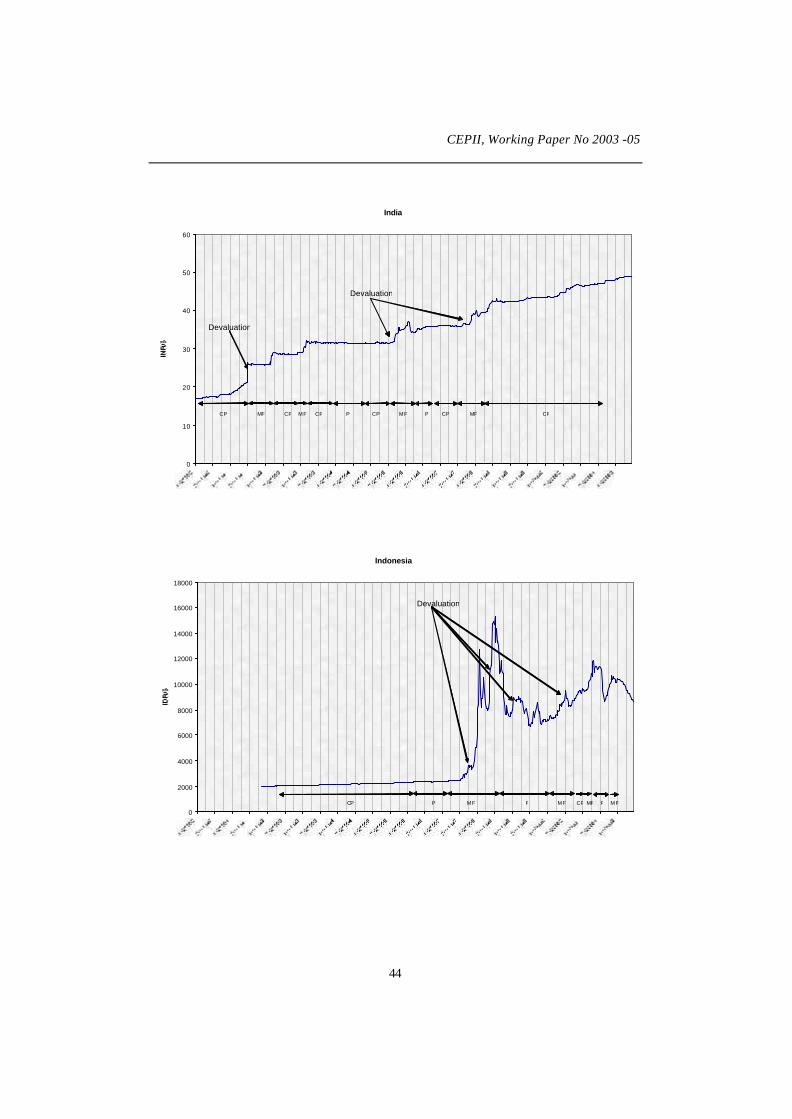
CEPII, Working Paper No 2003 -05
44
India
0
10
20
30
40
50
60
CP MF CP P CP MF P CP MF CPMF CP
Devaluation
Devaluation
Indonesia
0
2000
4000
6000
8000
10000
12000
14000
16000
18000
CP P MF F MF CP MF F MF
Devaluation

Does Exchange Rate Regime Explain Differences in Economic Results for Asian Countries ?
45
Korea
0
200
400
600
800
1000
1200
1400
1600
1800
2000
CP MF P MF CP MF F P CP MFF F P
Devaluation
Malaysia
1
1,5
2
2,5
3
3,5
4
4,5
5
P F P MF P MF F P
Devaluation

CEPII, Working Paper No 2003 -05
46
Pakistan
0
10
20
30
40
50
60
70
CP MF P CP MF CP MF CP MFCP MF MFMF CP CP
Devaluation
Philippines
10
15
20
25
30
35
40
45
50
55
60
MF CP P MF FC
PMF C
PMF C MF C F C MF C MF C
Devaluation
Devaluation
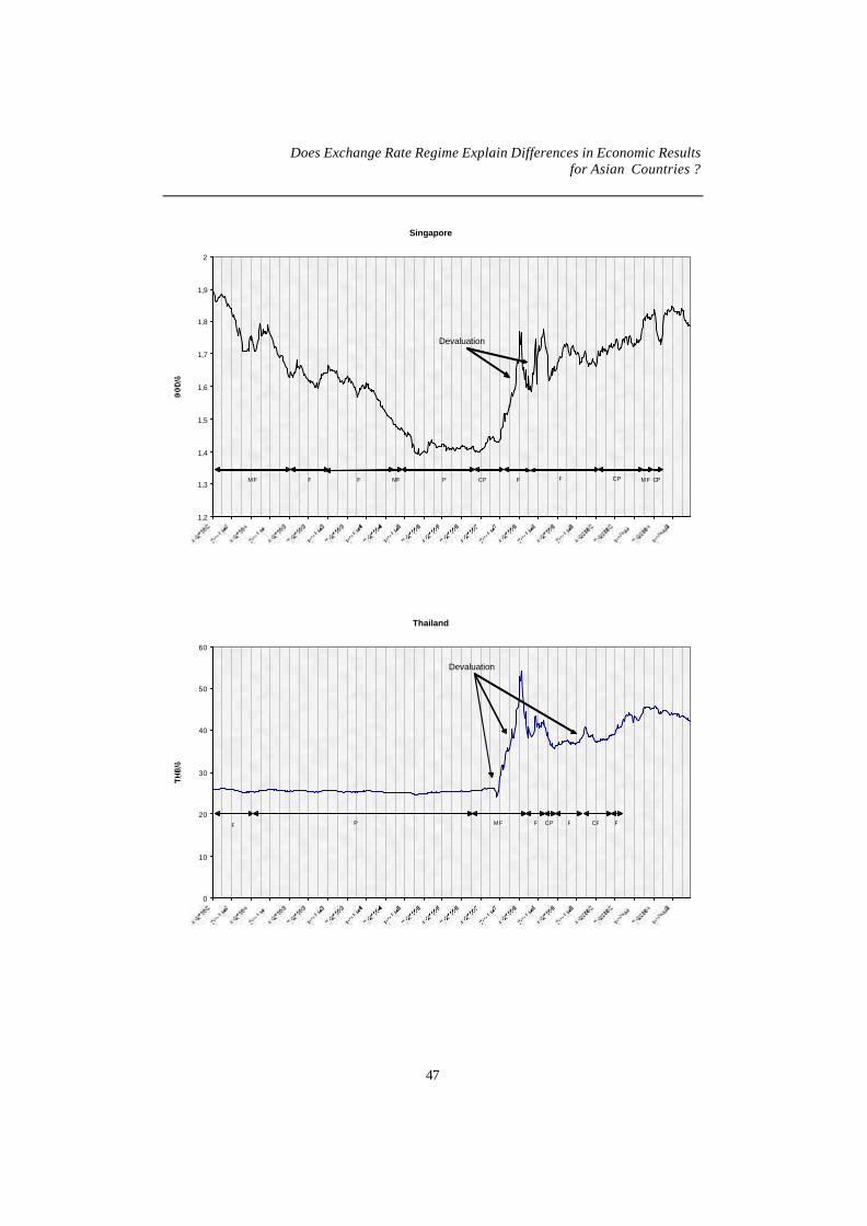
Does Exchange Rate Regime Explain Differences in Economic Results for Asian Countries ?
47
Singapore
1,2
1,3
1,4
1,5
1,6
1,7
1,8
1,9
2
MF P F P CP F P MFCP CPMF
Devaluation
Thailand
0
10
20
30
40
50
60
F P MF F CP F CP F
Devaluation
CEPII, Working Paper No 2003 -05
48
LIST OF WORKING PAPERS RELEASED BY CEPII5
No Title Authors
2004-04 Trade in the Triad: How Easy is the Access to LargeMarkets
L. Fontagné, T. Mayer& S. Zignago
2004-03 Programme de travail du CEPII pour 2004
2004-02 Technology Differences, Institutions and EconomicGrowth: a Conditional Conditional Convergence
H. Boulhol
2004-01 Croissance et régimes d’investissement P. Villa
2003-22 A New Look at the Feldstein-Horioka Puzzle using anIntegrated Panel
A. Banerjee & P.Zanghieri
2003-21 Trade Linkages and Exchange Rates in Asia: The Roleof China
A. Bénassy-Quéré &A. Lahrèche-Révil
2003-20 Economic Implications of Trade Liberalization Underthe Doha Round
J. Francois,H. Van Meijl,
F. Van Tongeren2003-19 Methodological Tools for SIA – Report of the CEPII
Worshop held on 7-8 November 2002 in BrusselsN. Kousnetzoff
2003-18 Order Flows, Delta Hedging and Exchange RateDynamics
B. Rzepkowski
2003-17 Tax competition and Foreign Direct Investment A. Bénassy-Quéré,L. Fontagné & A.
Lahrèche-Révil
2003-16 Commerce et transfert de technologies : les cascomparés de la Turquie, de l’Inde et de la Chine
F. Lemoine &D. Ünal-Kesenci
2003-15 The Empirics of Agglomeration and Trade K. Head & T. Mayer
2003-14 Notional Defined Contribution: A Comparison of theFrench and German Point Systems
F. Legros
2003-13 How Different is Eastern Europe? Structure andDeterminants of Location Choices by French Firms inEastern and Western Europe
C. Disdier &T. Mayer
2003-12 Market Access Liberalisation in the Doha Round: L. Fontagné, J.L.
5 Working papers are circulated free of charge as far as stocks are available; thank you to send your request
to CEPII, Sylvie Hurion, 9, rue Georges-Pitard, 75015 Paris, or by fax : (33) 01 53 68 55 04 or by [email protected]. Also available on: \\www.cepii.fr. Working papers with * are out of print. They cannevertheless be consulted and downloaded from this website.5 Les documents de travail sont diffusés gratuitement sur demande dans la mesure des stocks disponibles.
Merci d’adresser votre demande au CEPII, Sylvie Hurion, 9, rue Georges-Pitard, 75015 Paris, ou parfax : (33) 01 53 68 55 04 ou par e-mail [email protected]. Egalement disponibles sur : \\www.cepii.fr.Les documents de travail comportant * sont épuisés. Ils sont toutefois consultable sur le web CEPII.

Does Exchange Rate Regime Explain Differences in Economic Results for Asian Countries ?
49
Scenarios and Assessment Guérin & S. Jean
2003-11 On the Adequacy of Monetary Arrangements in Sub-Saharian Africa
A. Bénassy-Quéré &Maylis Coupet
2003-10 The Impact of EU Enlargement on Member States : aCGE Approach
H. Bchir, L. Fontagné& P. Zanghieri
2003-09 India and the World Economy : TraditionalSpecialisations and Technology Niches
S. Chauvin &F. Lemoine
2003-08 Imination Amongst Exchange-Rate Forecasters :Evidence from Survey Data
M. Beine,A. Bénassy-Quéré &
H. Colas
2003-07 Le Currency Board à travers l’expérience del’Argentine
S. Chauvin & P. Villa
2003-06 Trade and Convergence : Revisiting Ben-David G. Gaulier
2003-05 Estimating the Fundamental Equilibrium Exchange-Rate of Central and Eastern European Countries theEMU Enlargement Perspective
B Egert &A. Lahrèche-Revil
2003-04 Skills, Technology and Growth is ICT the Key toSuccess
J. Melka, L. Nayman,S. Signano &
N. Mulder
2003-03 L’investissement en TIC aux Etats-Unis et dansquelques pays européens
G. Cette & P.A. Noual
2003-02 Can Business and Social Networks Explain the BorderEffect Puzzle?
P.P. Combes,M. Lafourcade &
T. Mayer2003-01 Hyperinflation and the Reconstruction of a National
Money: Argentina and Brazil, 1990-2002J. Sgard
2002-18 Programme de travail du CEPII pour 2003
2002-17 MIRAGE, a Computable General Equilibrium Modelfor Trade Policy Analysis
M.H. Bchir,Y. Decreux,
J.L. Guérin & S. Jean2002-16 Evolutions démographiques et marché du travail : des
liens complexes et parfois contradictoiresL. Cadiou, J. Genet &
J.L. Guérin
2002-15 Exchange Rate Regimes and Sustainable Parities forCEECs in the Run-up to EMU Membership
V. Coudert &C. Couharde
2002-14 When are Structural Deficits Good Policies? J. Chateau
2002-13 Projections démographiques de quelques pays del’Union Européenne (Allemagne, France, Italie,Royaume-Uni, Pays-Bas, Suède)
R. Sleiman
2002-12 Regional Trade Integration in Southern Africa S. Chauvin &G. Gaulier

CEPII, Working Paper No 2003 -05
50
2002-11 Demographic Evolutions and Unemployment: anAnalysis of French Labour Market with WorkersGenerations
J. Château, J.L. Guérin& F. Legros
2002-10 Liquidité et passage de la valeur P. Villa
2002-09 Le concept de coût d’usage Putty-Clay des biensdurables
M.G. Foggea &P. Villa
2002-08 Mondialisation et régionalisation : le cas des industriesdu textile et de l’habillement
M. Fouquin, P. MorandR. Avisse G. Minvielle
& P. Dumont2002-07 The Survival of Intermediate Exchange Rate Regimes A. Bénassy-Quéré &
B. Coeuré2002-06 Pensions and Savings in a Monetary Union : An
Analysis of Capital FlowA. Jousten & F. Legros
2002-05 Brazil and Mexico’s Manufacturing Performance inInternational Perspective, 1970-1999
N. Mulder, S. Montout& L. Peres Lopes
2002-04 The Impact of Central Bank Intervention onExchange-Rate Forecast Heterogeneity
M. Beine,A. Benassy-Quéré,
E. Dauchy &R. MacDonald
2002-04 The Impact of Central Bank Intervention on ForecastHeterogeneity
M. Beine,A. Benassy-Quéré,
E. Dauchi &R. MacDonald
2002-03 Impacts économiques et sociaux de l’élargissementpour l’Union européenne et la France
M.H. Bchir &M. Maurel
2002-02 China in the International Segmentation of ProductionProcesses
F. Lemoine &D. Ünal-Kesenci
2002-01 Illusory Border Effects: Distance MismeasurementInflates Estimates of Home Bias in Trade
K Head & T. Mayer
2001-22 Programme de travail du CEPII pour 2002
2001-21 Croissance économique mondiale : un scénario deréférence à l’horizon 2030
N. Kousnetzoff
2001-20 The Fiscal Stabilization Policy under EMU – AnEmpirical Assessment
A. Kadareja
2001-19 Direct Foreign Investments and Productivity Growthin Hungarian Firms, 1992-1999
J. Sgard
2001-18 Market Access Maps: A Bilateral and DisaggregatedMeasure of Market Access
A. Bouët, L. Fontagné,M. Mimouni &
X. Pichot
2001-17 Macroeconomic Consequences of Pension Reforms inEurope: An Investigation with the INGENUE WorldModel
Equipe Ingénue
Does Exchange Rate Regime Explain Differences in Economic Results for Asian Countries ?
51
2001-16* La productivité des industries méditerranéennes A. Chevallier &D. Ünal-Kesenci
2001-15 Marmotte: A Multinational Model L. Cadiou, S. Dees,S. Guichard,A. Kadareja,
J.P. Laffargue &B. Rzepkowski
2001-14 The French-German Productivity ComparisonRevisited: Ten Years After the German Unification
L. Nayman &D. Ünal-Kesenci
2001-13* The Nature of Specialization Matters for Growth: AnEmpirical Investigation
I. Bensidoun,G. Gaulier
& D. Ünal-Kesenci
2001-12 Forum Economique Franco-Allemand - Deutsch-Französisches Wirtschaftspolitisches Forum, PoliticalEconomy of the Nice Treaty: Rebalancing the EUCouncil and the Future of European AgriculturalPolicies, 9th meeting, Paris, June 26th 2001
2001-11 Sector Sensitivity to Exchange Rate Fluctuations M. Fouquin, K. Sekkat,J. Malek Mansour,
N. Mulder &L. Nayman
2001-10* A First Assessment of Environment-Related TradeBarriers
L. Fontagné, F. vonKirchbach &M. Mimouni
2001-09 International Trade and Rend Sharing in Developedand Developing Countries
L. Fontagné &D. Mirza
2001-08 Economie de la transition : le dossier G. Wild
2001-07 Exit Options for Argentina with a Special Focus onTheir Impact on External Trade
S. Chauvin
2001-06 Effet frontière, intégration économique et 'ForteresseEurope'
T. Mayer
2001-05 Forum Économique Franco-Allemand – Deutsch-Französisches Wirtschaftspolitisches Forum, TheImpact of Eastern Enlargement on EU-LabourMarkets and Pensions Reforms between Economicand Political Problems, 8th meeting, Paris, January 162001
2001-04 Discrimination commerciale : une mesure à partir desflux bilatéraux
G. Gaulier
2001-03* Heterogeneous Expectations, Currency Options andthe Euro/Dollar Exchange Rate
B. Rzepkowski

CEPII, Working Paper No 2003 -05
52
2001-02 Defining Consumption Behavior in a Multi-CountryModel
O. Allais, L. Cadiou &S. Dées
2001-01 Pouvoir prédictif de la volatilité implicite dans le prixdes options de change
B. Rzepkowski
2000-22 Forum Economique Franco-Allemand - Deutsch-Französisches Wirtschaftspolitisches Forum, TradeRules and Global Governance: A long Term Agendaand The Future of Banking in Europe, 7th meeting,Paris, July 3-4 2000
2000-21 The Wage Curve: the Lessons of an Estimation Over aPanel of Countries
S. Guichard &J.P. Laffargue
2000-20 A Computational General Equilibrium Model withVintage Capital
L. Cadiou, S. Dées &J.P. Laffargue
2000-19 Consumption Habit and Equity Premium in the G7Countries
O. Allais, L. Cadiou &S. Dées
2000-18 Capital Stock and Productivity in French Transport:An International Comparison
B. Chane Kune &N. Mulder
2000-17 Programme de travail 2001
2000-16 La gestion des crises de liquidité internationale :logique de faillite, prêteur en dernier ressort etconditionnalité
J. Sgard
2000-15 La mesure des protections commerciales nationales A. Bouët
2000-14 The Convergence of Automobile Prices in theEuropean Union: An Empirical Analysis for thePeriod 1993-1999
G. Gaulier & S. Haller
2000-13* International Trade and Firms’ Heterogeneity UnderMonopolistic Competition
S. Jean
2000-12 Syndrome, miracle, modèle polder et autresspécificités néerlandaises : quels enseignements pourl’emploi en France ?
S. Jean
2000-11 FDI and the Opening Up of China’s Economy F. Lemoine
2000-10 Big and Small Currencies: The Regional Connection A. Bénassy-Quéré &B. Coeuré
2000-09* Structural Changes in Asia And Growth ProspectsAfter the Crisis
J.C. Berthélemy &S. Chauvin
2000-08 The International Monetary Fund and the InternationalFinancial Architecture
M. Aglietta
2000-07 The Effect of International Trade on Labour-DemandElasticities: Intersectoral Matters
S. Jean

Does Exchange Rate Regime Explain Differences in Economic Results for Asian Countries ?
53
2000-06 Foreign Direct Investment and the Prospects for TaxCo-Ordination in Europe
A. Bénéssy-Quéré,L. Fontagné &
A. Lahrèche-Révil
2000-05 Forum Economique Franco-Allemand - Deutsch-Französisches Wirtschaftspolitisches Forum,Economic Growth in Europe Entering a NewArea?/The First Year of EMU, 6th meeting, Bonn,January 17-18, 2000
2000-04* The Expectations of Hong Kong Dollar Devaluationand their Determinants
B. Rzepkowski
2000-03 What Drove Relative Wages in France? StructuralDecomposition Analysis in a GeneralEquilibrium Framework, 1970-1992
S. Jean & O. Bontout
2000-02 Le passage des retraites de la répartition à lacapitalisation obligatoire : des simulations à l’aided’une maquette
O. Rouguet & P. Villa
2000-01* Rapport d’activité 1999
1999-16 Exchange Rate Strategies in the Competition forAttracting FDI
A. Bénassy-Quéré,L. Fontagné &
A. Lahrèche-Révil
1999-15 Groupe d’échanges et de réflexion sur la Caspienne.Recueil des comptes-rendus de réunion (déc. 97- oct.98)"
D. Pianelli &G. Sokoloff
1999-14 The Impact of Foreign Exchange Interventions: NewEvidence from FIGARCH Estimations
M. Beine,A. Bénassy-Quéré &
C. Lecourt
1999-13 Forum Economique Franco-Allemand - Deutsch-Französisches Wirtschaftspolitisches Forum,Reduction of Working Time/Eastward Enlargment ofthe European Union, 5 th meeting, Paris, July 6-7 1999
1999-12* A Lender of Last Resort for Europe M. Aglietta
1999-11* La diversité des marchés du travail en Europe :Quelles conséquences pour l’Union Monétaire ;Deuxième partie : Les implications macro-économiques de la diversité des marchés du travail
L. Cadiou, S. Guichard& M. Maurel
1999-10* La diversité des marchés du travail en Europe :Quelles conséquences pour l’Union Monétaire ;Première partie : La diversité des marchés du travaildans les pays de l’Union Européenne
L. Cadiou &S. Guichard
1999-09 The Role of External Variables in the ChineseEconomy; Simulations from a macroeconometric
S. Dees

CEPII, Working Paper No 2003 -05
54
model of China
1999-08 Haute technologie et échelles de qualité : de fortesasymétries en Europe
L. Fontagné,M. Freudenberg &
D. Ünal-Kesenci
1999-07 The Role of Capital Accumultion, Adjustment andStructural Change for Economic Take-Off: EmpiricalEvidence from African Growth Episodes
J.C. Berthélemy &L. Söderling
1999-06 Enterprise Adjustment and the Role of Bank Credit inRussia: Evidence from a 420 Firm’s QualitativeSurvey
S. Brana, M. Maurel &J. Sgard
1999-05 Central and Eastern European Countries in theInternational Division of Labour in Europe
M. Freudenberg &F. Lemoine
1999-04 Forum Economique Franco-Allemand – EconomicPolicy Coordination – 4 th meeting, Bonn, January 11-12 1999
1999-03 Models of Exchange Rate Expectations:Heterogeneous Evidence From Panel Data
A. Bénassy-Quéré,S. Larribeau &R. MacDonald
1999-02 Forum Economique Franco-Allemand – LabourMarket & Tax Policy in the EMU
1999-01 Programme de travail 1999


CEPIIDOCUMENTS DE TRAVAIL / WORKING PAPERS
Si vous souhaitez recevoir des Documents de travail,merci de remplir le coupon-réponse ci-joint et de le retourner à :
Should you wish to receive copies of the CEPII’s Working papers,just fill the reply card and return it to:
Sylvie HURION – PublicationsCEPII – 9, rue Georges-Pitard – 75740 Paris – Fax : (33) 1.53.68.55.04
M./Mme / Mr./Mrs ................................................................................................................................
Nom-Prénom / Name-First name .........................................................................................................
Titre / Title ...............................................................................................................................................
Service / Department..............................................................................................................................
Organisme / Organisation .....................................................................................................................
Adresse / Address...................................................................................................................................
Ville & CP / City & post code .............................................................................................................Pays / Country...................................................................... Tél. ...........................................................
Désire recevoir les Document de travail du CEPII n° :
Wish to receive the CEPII’s Working Papers No: ..........................................................................
...................................................................................................................................................................
...................................................................................................................................................................
...................................................................................................................................................................
...................................................................................................................................................................
...................................................................................................................................................................
...................................................................................................................................................................
...................................................................................................................................................................
c Souhaite être placé sur la liste de diffusion permanente (pour les bibliothèques)Wish to be placed on the standing mailing list (for Libraries).