NBER WORKING PAPER SERIES

DOES HIGH HOME-OWNERSHIP IMPAIR THE LABOR MARKET?

David G. BlanchflowerAndrew J. Oswald

Working Paper 19079http://www.nber.org/papers/w19079

NATIONAL BUREAU OF ECONOMIC RESEARCH1050 Massachusetts Avenue

Cambridge, MA 02138May 2013

For suggestions and valuable discussion, we thank seminar participants at PIIE and Dean Baker, HankFarber, William Fischel, Barry McCormick, Ian M. McDonald, Michael McMahon, Robin Naylor,Jeremy Smith, Doug Staiger, Rob Valletta, and Thijs van Rens. The views expressed herein are thoseof the authors and do not necessarily reflect the views of the National Bureau of Economic Research.

At least one co-author has disclosed a financial relationship of potential relevance for this research.Further information is available online at http://www.nber.org/papers/w19079.ack

NBER working papers are circulated for discussion and comment purposes. They have not been peer-reviewed or been subject to the review by the NBER Board of Directors that accompanies officialNBER publications.

© 2013 by David G. Blanchflower and Andrew J. Oswald. All rights reserved. Short sections of text,not to exceed two paragraphs, may be quoted without explicit permission provided that full credit,including © notice, is given to the source.

Does High Home-Ownership Impair the Labor Market?David G. Blanchflower and Andrew J. OswaldNBER Working Paper No. 19079May 2013JEL No. J01,J6

ABSTRACT

We explore the hypothesis that high home-ownership damages the labor market. Our results are relevantto, and may be worrying for, a range of policy-makers and researchers. We find that rises in the home-ownership rate in a U.S. state are a precursor to eventual sharp rises in unemployment in that state.The elasticity exceeds unity: a doubling of the rate of home-ownership in a U.S. state is followed inthe long-run by more than a doubling of the later unemployment rate. What mechanism might explainthis? We show that rises in home-ownership lead to three problems: (i) lower levels of labor mobility,(ii) greater commuting times, and (iii) fewer new businesses. Our argument is not that owners themselvesare disproportionately unemployed. The evidence suggests, instead, that the housing market can producenegative ‘externalities’ upon the labor market. The time lags are long. That gradualness may explainwhy these important patterns are so little-known.

David G. BlanchflowerBruce V. Rauner Professor of Economics6106 Rockefeller HallDartmouth CollegeHanover, NH 03755-3514and NBERDavid.G.Blanchflower@Dartmouth.EDU

Andrew J. OswaldDepartment of Economicsand also CAGE Research Center University of WarwickCoventry CV4 7ALEnglanda.j.oswald@warwick.ac.uk

1

Does High Home-Ownership Impair the Labor Market?

David G. Blanchflower Andrew J. Oswald

1. Introduction

Unemployment is a major source of unhappiness, mental ill-health, and lost income.1 Yet after a

century of economic research on the topic, the determinants of the equilibrium or ‘natural’ rate

of unemployment are still imperfectly understood, and unemployment levels in the industrialized

nations are today 10%, with some nations over 20%.2 The historical focus of the research

literature has been on which labor-market characteristics -- trade unionism, unemployment

benefits, job protection, etc -- are particularly influential.

We propose a different approach to the problem. Our study provides evidence consistent

with the view that the housing market plays a fundamental role as a determinant of the rate of

unemployment. We study modern and historic data from the United States. We construct state

panels, and then estimate unemployment equations.3 Using data on two million randomly

sampled Americans, we also estimate equations for the number of weeks worked, the extent of

labor mobility, the length of commuting times, and the number of businesses. Our results seem

relevant to, and should perhaps be seen as worrying for, a wide range of policy-makers and

researchers. There are four main conclusions. First, we document a strong statistical link

1 Linn et al. (1985), DiTella et al. (2003), Murphy and Athanasou (1999), Paul and Moser (2009), and Powdthavee (2010), for example. 2 The Euro Area unemployment rate for December 2012 was 11.7%, ranging from a low of 4.3% in Austria, 5.3% in Germany, and 5.8% in the Netherlands, up to a high of 26.8% in Greece and 26.1% in Spain, who both had youth unemployment rates of >50%. France had a rate of 10.6% and Italy 10.9%, while the UK and the USA both had unemployment rates of 7.8%. http://epp.eurostat.ec.europa.eu/cache/ITY_PUBLIC/3-01022013-BP/EN/3-01022013-BP-EN.PDF 3 Our work builds upon a tradition of labor-market research with state panels from the 1990s in sources such as Blanchard and Katz (1992) and Blanchflower and Oswald (1994).

2

between high levels of home-ownership in a geographical area and high later levels of

joblessness in that area. We show that this result is robust across sub-periods going back to the

1980s. The lags from ownership levels to unemployment levels are long. They can take up to

five years to be evident. This suggests that high home-ownership may gradually interfere with

the efficient functioning of a labor market. Second, we show that, both within states and across

states, high home-ownership areas have lower labor mobility. Importantly, this is not due

merely to the personal characteristics of owners and renters. We are unable, in this paper, to say

exactly why, or to give a complete explanation for the patterns that are found, but our study’s

results are consistent with the unusual idea that the housing market can create dampening

externalities upon the labor market and the economy. Third, we show that states with higher

rates of home-ownership have longer commute times. This phenomenon is likely to be a

reflection of the greater transport congestion that goes with a less mobile workforce and it will

act to raise costs for employers and employees. Fourth, we demonstrate that states with higher

rates of home-ownership have lower rates of business formation. This might be the result of

zoning restrictions and NIMBY effects of a kind that, as Fischel (2004) discusses, are rational

for home-owners. But currently that channel can be only a conjecture.

The data used in this paper are almost wholly from the United States. However, our

conclusions may have wider implications. Taken in conjunction with new work by Laamanen

(2013), which was done independently of our own4, and reaches similar conclusions for the

country of Finland, the findings may go some way to explain why nations like Spain (80%

owners, 20+% unemployment) and Switzerland (30% owners, 3% unemployment) can have

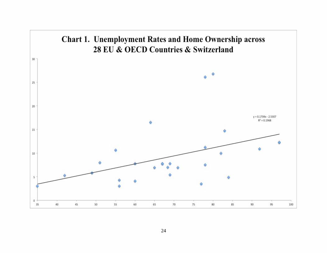
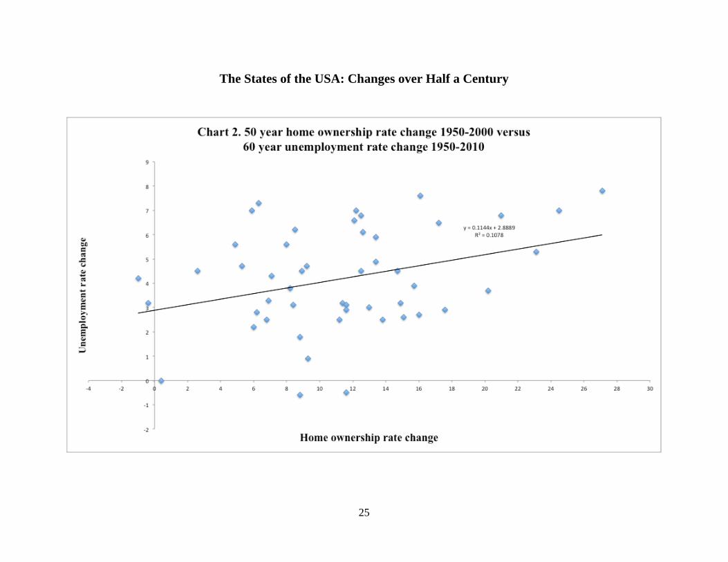
such different mixtures of home-ownership and joblessness. Chart 1 shows that there is a strong

4 In April 2013, Laanamen and Blanchflower-Oswald discovered they had equivalent empirical findings, though done in different ways, for Finland and the USA respectively.

3

positive correlation across the wealthy countries between their home-ownership rates and the

latest unemployment rates. Such a chart is open to the sensible criticism that the scatter might be

an illusion caused by country fixed-effects. However, that objection cannot be raised about

Chart 2, which is for the United States. It plots very long changes (approximately half-century

changes) in home-ownership rates and unemployment rates across the US states – minus Alaska

and Hawaii – and generates a similar result. It plots the fifty-year change in home-ownership

rates (1950-2000) against a sixty-year change in unemployment rates (1950-2010).5

The later analysis does not depend on data from the special period of the 2007 US house-

price crash;6 nor does it rely on the idea that home owners are themselves disproportionately

unemployed (there is a considerable literature that suggests such a claim is false, or, at best,

weak); nor does it imply that spatial compensating differentials theory is incorrect; nor is it

Keynesian in spirit7; nor does it rest upon the idea of ‘house-lock’ in a housing downturn (for

example, Ferreira et al. 2010, Valletta 2012). Our paper makes a simple statistical contribution

and discusses possible mechanisms. The detailed nature of any housing-labor externality remains

poorly understood.

2. Background

In his 1968 address to the American Economic Association, Milton Friedman famously

argued that the natural rate of unemployment can be expected to depend upon the degree of labor

5 Source for the 1950 state unemployment rates is http://www.census.gov/prod/www/abs/decennial/1950cenpopv2.html 6 Repercussions from the worldwide house-price bubble are discussed in sources such as Bell and Blanchflower (2010) and Dickens and Triest (2012). 7 We would like to acknowledge valuable discussions with Ian McDonald on this issue. One reason why our effect does not appear to be consistent with a Keynesian argument is that we find the lags from home-ownership are long, and that is inconsistent with the idea that our estimated unemployment effect in time t is the result of aggregate demand in time t.

4

mobility in the economy. The functioning of the labor market will thus be shaped not just by

long-studied factors such as the generosity of unemployment benefits and the strength of trade

unions,8 but also by the nature, and inherent flexibility and dynamism of, the housing market.

However, on that topic there has been relatively little empirical research.

One important early line of work stemmed from scholars such as McCormick (1983) and

Hughes and McCormick (1981). This found evidence that in certain types of public-sector

housing the degree of labor mobility was low and the associated joblessness was high9. That

research tradition still continues -- as in Dujardin and Goffette-Nagot (2009). A broader

literature at the border between labor and urban economics has considered whether there might

be fundamental differences in the labor-market impact of renting rather than owning. Some of

this work was triggered by the suggestion in a public lecture by Oswald (1996, 1997) that,

especially in Europe, at the aggregate level a higher proportion of home-ownership (or ‘owner-

occupation’) seems to be associated empirically with a larger amount of unemployment.

Oswald’s data were mainly for the western nations and for the states of the USA. He presented

no formal regression equations. Green and Hendershott (2001) subsequently reported US

econometric results that were somewhat, though not entirely, supportive.

One theoretical interpretation of these early patterns was that home-ownership might

raise unemployment by slowing the ability of jobless owners to move to new opportunities. In

response to this idea, a number of researchers later examined micro data. The ensuing literature

concluded that the bulk of the evidence is against the idea that home-owning individuals are

8 For example, OECD (1994) and Layard et al. (1991). 9 McCormick (1983) makes the interesting point that economists should not work on the assumption that low mobility is always undesirable. If home ownership facilitates the accumulation of wealth, and wealth has a negative

5

unemployed more than renters. Hence -- though the empirical debate continues -- a number of

authors concluded that Oswald’s general idea must be incorrect and the cross-country pattern

must be illusory. A modern literature includes Battu et al. (2008), Coulson and Fisher (2002,

2009), Dohmen (2005), Head and Lloyd-Ellis (2012), Van Leuvensteijn and Koning (2004),

Munch et al. (2006), Rouwendal and Nijkamp (2010), Smith and Zenou (2003), and Zabel

(2012).

An alternative possibility -- one that has not, to our knowledge, been fully explored

empirically -- is the hypothesis that the housing market might create externalities. There are a

number of ways in which such spillovers might operate. For example, Serafinelli (2012) shows

in the US labor market that there appear to be beneficial informational externalities upon

workers’ productivity from a high degree of labor mobility. Although the author does not pursue

the implication, this raises the possibility that any housing market structure that led to

immobility could, therefore, produce negative externalities on workers and firms. Oswald

(1999) suggests a different possible channel. Homeowners might act to hold back development

in their area (through zoning restrictions) in a way that could be detrimental to new jobs and

entrepreneurial ventures. This would be NIMBY pressures -- not in my back yard -- in action.

A third possibility is that regions with high home-ownership might be difficult ones in which to

attract migrant workers (who may require the flexibility of rental accommodation). As a fourth

possibility, a formal model in the literature by Dohmen (2005) predicts that high ownership can

be associated with high unemployment. The reason, within Dohmen’s framework, is not one

linked to an externality but instead to the fact that the composition of the unemployed pool is

endogenous to the structure of the housing market (in other words, the kind of person who is

effect on migration rates, then a migration cost arises which will and should influence migration and hence unemployment rates, without necessarily doing 'bad things'.

6

unemployed alters when the home ownership rate goes up). None of these mechanisms requires

the homeowners themselves to be disproportionately unemployed (as in the critique of Munch et

al. 2006).

Most unemployment researchers begin from the tradition of neoclassical economics and

with the idea that there is some underlying equation, defined over tastes and technology, that

explains the structural or long-run rates of unemployment and employment. Whether from the

modern matching tradition due especially to researchers such as Mortensen and Pissarides

(1994), the 1990s macro-labor literature due especially to researchers such as Layard, Nickell

and Jackman (1991), or the classical literature that goes back at least to Pigou (1914), a huge

body of empirical work in economics has searched for labor market characteristics -- such as the

degree of trade unionism -- that might enter that natural-rate equation.

We wish to remain open-minded about the true model of the labor market. For a region’s

unemployment rate, we will think about this generically as an autoregressive relationship that

has a steady state solution, U*, which we will think of as the natural rate of unemployment. In

estimation, we can view the relevant equation as:

Unemployment rate in a region U(t) = f(U(t-1), labor market characteristics, housing market

characteristics, people’s demographic and educational characteristics, region characteristics,

year dummies)

We will add to the usual list of variables the rate of home-ownership in an area. For some

nations, it would be ideal to allow for a division of the housing market into three broad segments

7

– owners, private renters, and public-sector renters. In our empirical work, however, we use data

from the US, where public renting is sufficiently rare that it can be largely neglected.

3. Empirics

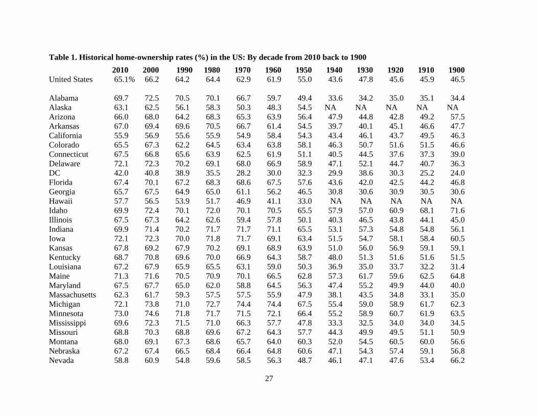
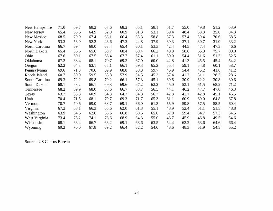
Tables 1 and 2 document the raw data. As implied by the earlier Chart 2, home-

ownership in the United States has grown strongly since 1900. It changed from a mean of

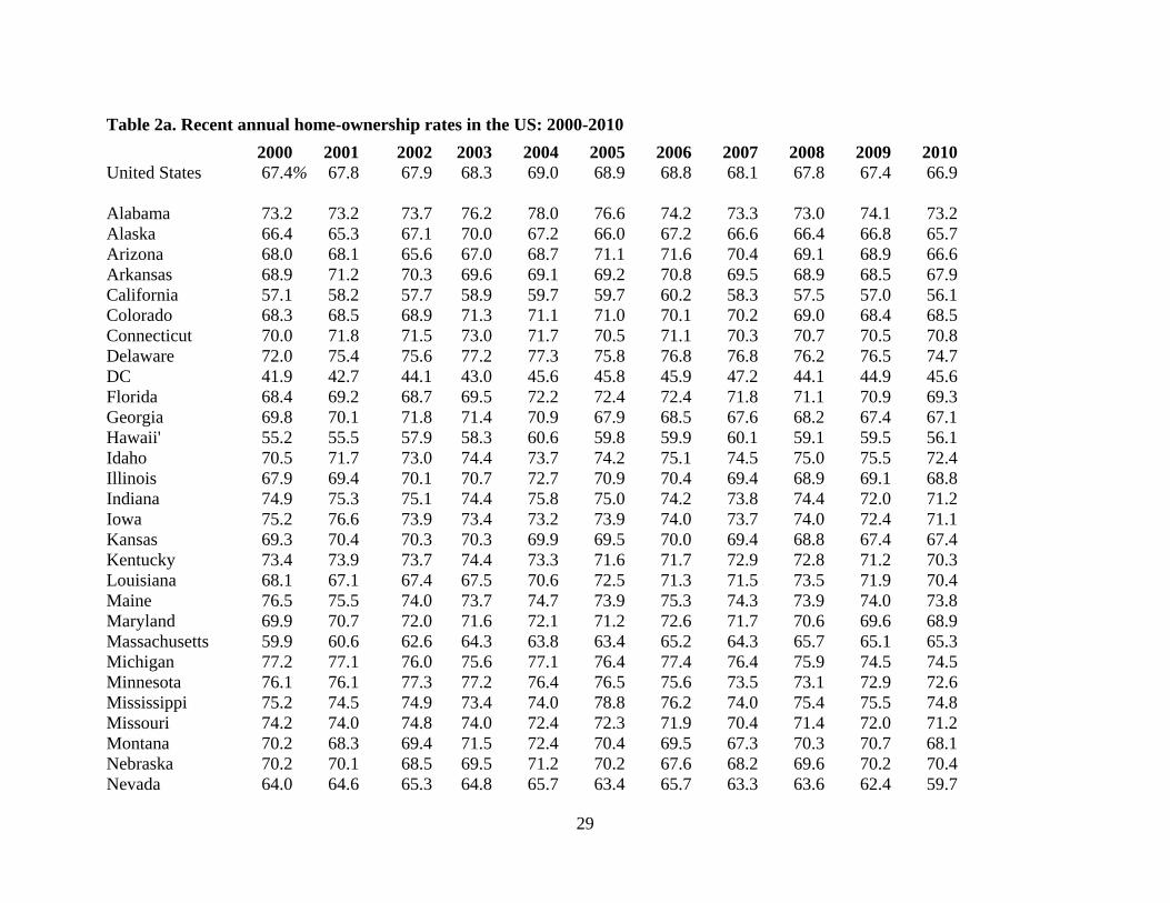
approximately 46% in that year to approximately 65% by the year 2010. Table 2 shows that the

US rate peaked in the year 2004, at 69%. This was a few years before the start of the infamous

modern housing crash. In 2010, the states of the US with the highest levels of home-ownership

were states such as Minnesota, Michigan, Delaware, and Iowa. The ownership levels were

lowest in states such as California and New York (and in DC if viewed as a state).10

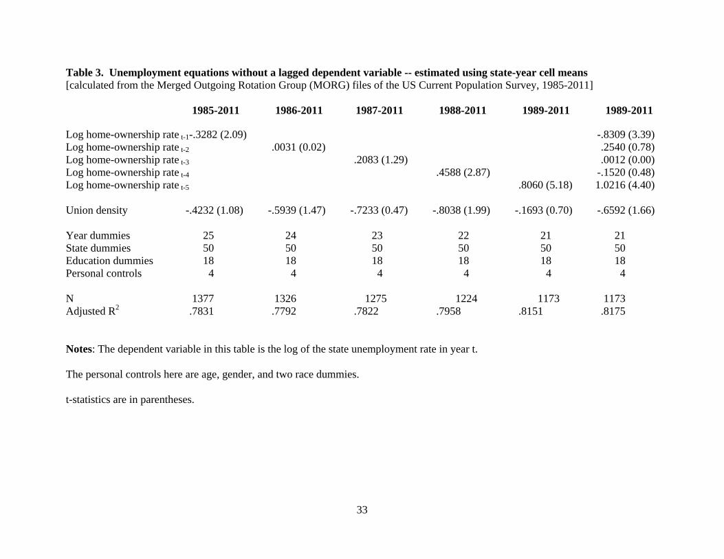
In Tables 3 and 4, we estimate unemployment equations. The estimation here is on an annual

panel of US states and uses as its dependent variable the natural logarithm of the state

unemployment rate. Our data cover a quarter of a century of consecutive years and are drawn

from the Merged Outgoing Rotation Groups of the Current Population Survey. The exact period

is 1985 to 2011, which gives us an effective sample size of 1377 area-time observations (that is,

of states by years). The different columns of Table 3 and 4 lay out a range of specifications,

including autoregressive specifications with a lagged dependent variable. Table 3 is presented

for intellectual completeness rather than because we believe it to be an adequate specification (a

lagged dependent variable enters strongly significantly, as would be expected, so Table 3 should

not be used to draw reliable inferences).

10 The most recent quarterly data on homeownership rates suggest that the decline may have slowed (%). Q1 Q2 Q3 Q4 Q1 Q2 Q3 Q4 2012 65.4 65.5 65.5 65.4 2008 67.8 68.1 67.9 67.5 2011 66.4 65.9 66.3 66.0 2007 68.4 68.2 68.2 67.8 2010 67.1 66.9 66.9 66.5 2006 68.5 68.7 69.0 68.9 2009 67.3 67.4 67.6 67.2 2005 69.1 68.6 68.8 69.0 http://www.census.gov/housing/hvs/files/qtr412/q412press.pdf

8

What emerges most clearly from Tables 3 and 4 is a correlation between unemployment in a

state in time t and the rate of home-ownership in that state in approximately year t-3 and earlier.

Summarizing, we find that unemployment:

Is higher in states that had high home-ownership rates in the past. The long-run elasticity

varies from 0.8 to 1.5. Given the context, these are large numbers.

Is autoregressive, with a coefficient on the lagged dependent variable Ut-1 of

approximately 0.8. Hence long-run effects are greatly magnified compared to the short-

run or ‘impact’ effect of the independent variable.

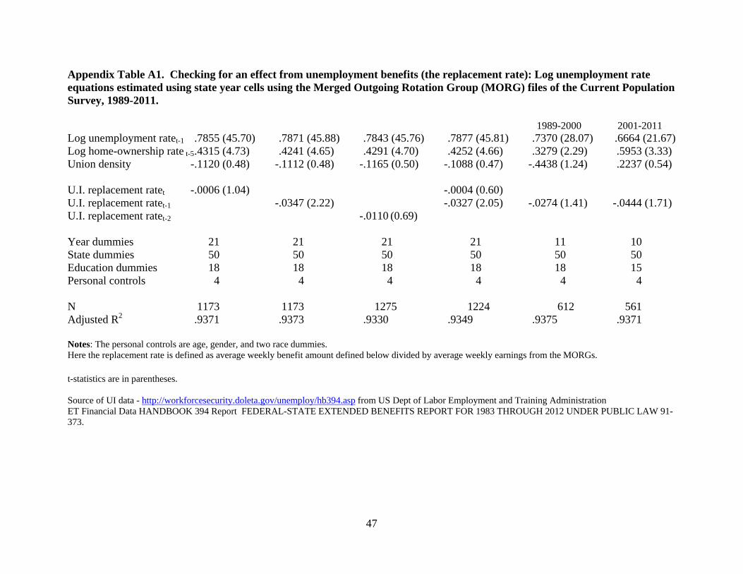
Is uncorrelated with union density in the state. The Appendix shows that that is also true

of (UI) unemployment insurance generosity.

Is correlated, as would be expected, with the personal characteristics of workers in the

state (the detailed results are not reported but follow the usual pattern of joblessness

being greater among those with fewer qualifications).

Is not significantly correlated with current home-ownership (the detailed results not

reported), which is why Tables 3 and 4 begin, in their respective column 1s, with an

ownership variable in time period t-1.

These judgments are from pooled cross-sections, so they describe associations in the data. We

should be cautious before imputing meaning into such patterns. Nevertheless, the fact that the

key correlation exists with a housing market variable so heavily lagged (back to t-5), and that the

regression equations control for state and year effects, suggests that the pattern is of interest and

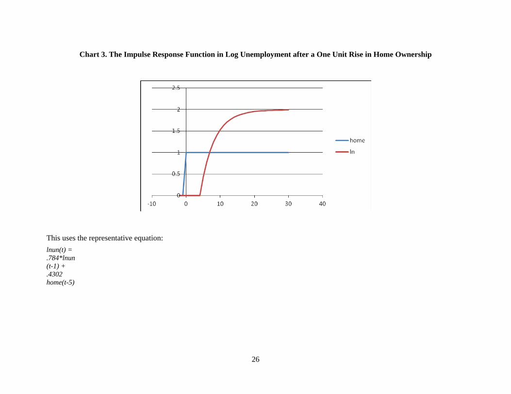
deserves to be taken seriously. Chart 3 plots the impulse-response function for one algebraic

example.

9

Table 3 contains the simplest results. In column 1, the home-ownership variable enters

negatively with a coefficient of -0.3282 and a t-statistic larger than two. If the underlying

economic prosperity in a state is captured in that year by data on either its current (high) home-

ownership rate, or by data on its (low) unemployment rate, a negative correlation here is not

surprising. Columns 2 and 3 of Table 3 then examine longer lags, and the ownership variable

becomes insignificantly different from zero.11

Columns 4, 5, and 6 of Table 3 contain results that are more remarkable. We see here

that the lagged home-ownership rate in the state becomes a powerful positive predictor of later

unemployment in that state. This finding is consistent with -- though it does not prove -- the

claim that, after some years have passed, a high degree of owner-occupation in an area can have

a deleterious structural effect on the labor market in that area. Table 3 reveals that the

coefficient on home-ownership in an unemployment equation becomes larger as the time lag

becomes longer. In column 5 of Table 3, the long-run ‘home-ownership elasticity of

unemployment’ is 0.8. These equations control for a number of independent influences on the

rate of joblessness. Importantly, both state and year dummies are included in the estimation.

Table 3 is useful for illustrative purposes but is not a natural or believable specification.

It is known that, presumably because unemployment is a stock variable and not a flow variable,

unemployment equations empirically are typically highly auto-regressive and thus (because

stocks are best characterized by differential equations) need to include a lagged dependent

variable. We now turn to that kind of specification.

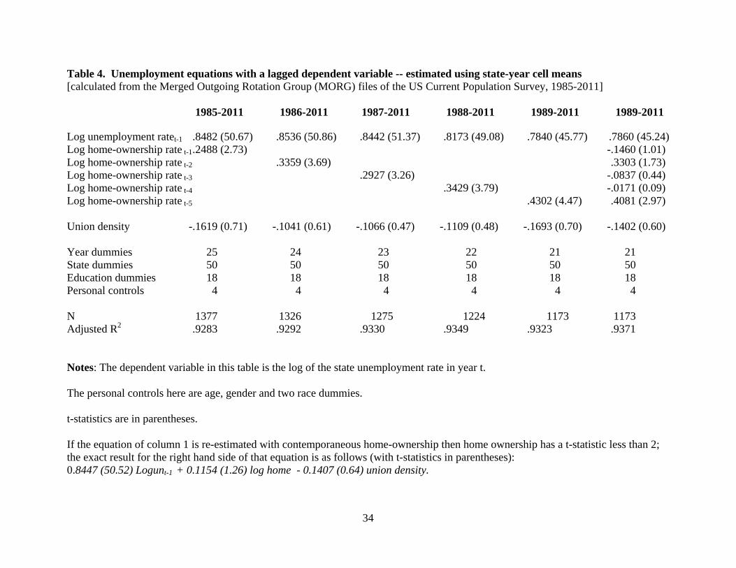
Table 4 contains the paper’s most important results. In the first column of Table 4, for

the entire period up to 2011, a lagged dependent variable has a coefficient of 0.8482 (with a t-

11 We experimented with clustering the standard errors at the level of the state in this and subsequent tables and the results were essentially unchanged.

10

statistic of approximately 50). Column 1 of Table 4 includes a set of year dummies; a set of

state dummies; 18 dummy variables for different levels, in the underlying micro data, of

people’s education; and controls for personal characteristics such as the average age of people in

the state. The unemployment rate in this form of panel is a slow-adjusting variable, and that

holds true despite the inclusion of state fixed effects. In this first column of Table 4 the

coefficient on lagged home-ownership is 0.2488. Here the lag is only a single year. The t-

statistic on this coefficient is 2.73, so the null hypothesis of a zero coefficient can be rejected at

conventional levels of confidence. The coefficient on union density has the wrong sign to be a

signal of any deleterious effect on joblessness; it is negative, with a t-statistic of only 0.71. 12

These estimates allow for adjustment for clustered standard errors.

Because this regression equation in column 1 of Table 4 is effectively a first-order

difference equation, the long-run home-ownership elasticity of unemployment is larger than the

impact effect of approximately 0.25. The long-run effect is, more precisely, 0.2488 divided by

(1.0000 – 0.8482). Hence the long run, or steady state, elasticity is estimated here at 1.7. In this

context, that is a surprisingly large number, and suggests the possibility that there are profound

connections between the workings of the US housing market and its labor market.

Interestingly, the size of the coefficient strengthens as we go further back. Column 2 of

Table 4 introduces a further lag on the home-ownership rate variable, namely, for ownership in

year t-2. It enters with a coefficient of 0.3359. The null hypothesis of zero can again be

rejected; the t-statistic is 3.69.

In columns 3, 4, and 5, respectively, further and further lags on home-ownership are

included. In the fifth column of Table 4, for example, the lagged dependent variable has a

12 In the appendix we also examine the impact of state unemployment benefits but can find no effect.

11

coefficient of 0.7840 and a coefficient on home-ownership in t-5 of 0.4302. The implied long

run elasticity is approximately 2.

The final column of Table 4 gives the fullest kind of specification where all home-

ownership rates are included from t-1 to t-5. The sum of these coefficients is approximately

0.49. The long run relationship thus continues to be a large one – in this case with a steady state

elasticity of 2.2.

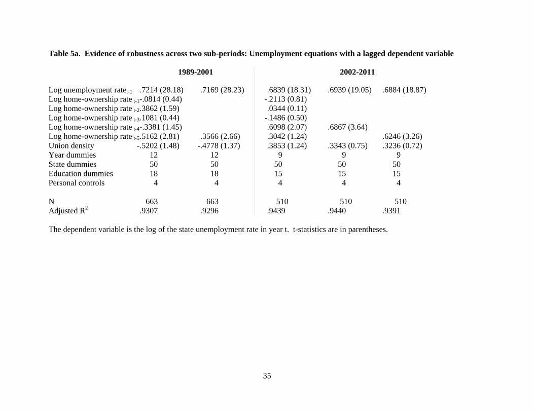
Is the pattern robust? Our experiments -- for example in Tables 5a and 5b -- suggest that

it is. First, it is conceivable that unemployment and home ownership simply both follow a state-

level business cycle but with different lagged timing. One way to probe for this is to replace the

state and year dummies with state time trends; it turns out that the results are then essentially

unchanged (results available on request).13 Splitting the data into two sub-periods, as in Table

5a, provides another illustration. It reveals the apparently reliability of the correlation between

the log of unemployment in period t and the log of home-ownership in a much earlier year. In

each of the two sub-periods in Table 5a, lagged home-ownership enters significantly. For the

period 1989-2001, the first segment of Table 5a estimates the coefficient on home-ownership in

t-5 at 0.3566. The coefficient on the lagged dependent variable in this estimated equation is

0.7169. Therefore the long-run home-ownership elasticity of unemployment is 1.3. In the later

period, the coefficient on ownership in t-5 is 0.6246, and the lagged dependent variable’s

coefficient is 0.6844. Then the long-run elasticity is 2.0.

13 Another possibility, suggested to us by Barry McCormick, is that both unemployment and home-ownership are driven by a common state level business cycle with different lag structures. Our correlation might then be illusory. We tested for this by estimating a series of state level home-ownership equations, which included long lags on both the log of the home ownership rate (5 lags) and the log of the unemployment rate (7 lags). There was no evidence of any effect from long lagged unemployment rates, which suggests that home-ownership here is not driven by local business cycles.

12

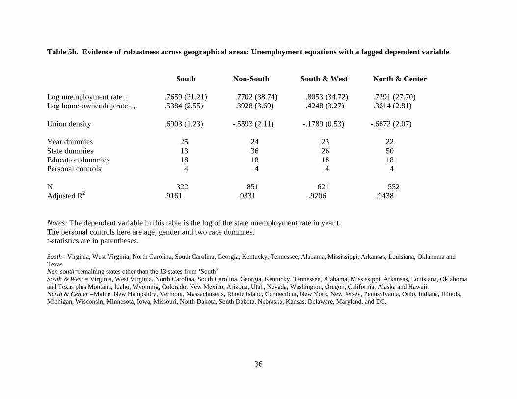
A different robustness test is presented in Table 5b. This is across different geographical

areas within the United States. Such a check seems important, because the South has had

particularly large rises in its home-ownership rate over the period, and our estimated home-

ownership effect might, in principle, be being driven in an illusory way solely by that part of the

country. Table 5b shows that that is not the case. The estimated equation exhibits a similar form

for a variety of geographical sub-divisions of the USA.

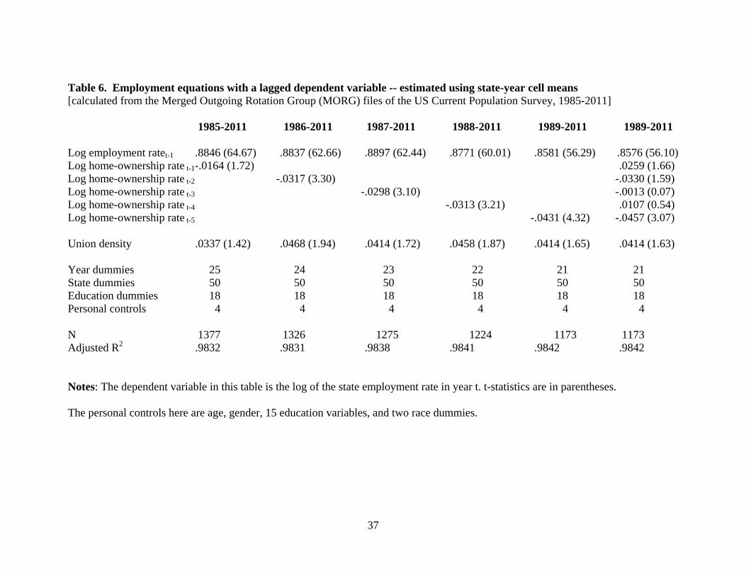
Some economists might prefer to focus on the level of employment as a key variable

rather than on the rate of joblessness itself. For that reason, Table 6 replicates the same general

finding using employment-rate, rather than unemployment-rate, data. Lagged home-ownership

rates enter strongly negatively in this state panel equation.

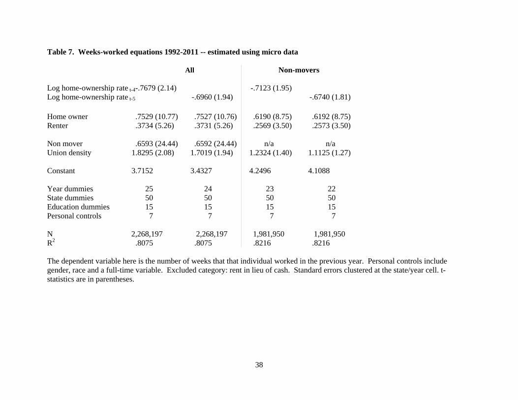
Table 7 tries a different check and turns to micro data on individual workers. It estimates

a weeks-worked equation using data from the March Current Population Surveys between 1992

and 2011. The sample size is approximately 2 million individuals. The dependent variable in

Table 7 is the number of weeks an individual worked during the previous year, rather than the

more usual 'point of time' measure of whether an individual was unemployed on the day they

were surveyed. Their answers are reported in 8 size bands in the data set; we allocated mid-

points. Non-workers were allocated zero weeks worked. In Table 7 we include controls for year

and state, as well as personal controls for race, gender and education, along with whether the

individual was a mover – defined as whether they changed their place of residence over the year

as well as if they primarily worked full-time and/or was a union member. In addition, we

include controls for whether the individual was a home owner or a renter (with the excluded

category being renters who received the accommodation for no charge). We also include the log

of the state*year home ownership rate, defined at the household level, lagged four years in

13

columns 1 and 3 and five years in columns 2 and 4. Separate results are presented for the full

sample as well as for the (vast) majority who were non-movers. Consistent with earlier results,

lagged home-ownership enters negatively with a large coefficient in Table 7 (though it hovers

close to the 95% cut-off level of confidence). It is thus associated with fewer weeks worked.

This is equivalent to our earlier finding: it seems to imply that the 'natural rate of employment' is

reduced by high ownership of homes. What is notable about Table 7 is that we are apparently

picking up deleterious effects on the labor market after controlling for the individual worker’s

own housing status (that is, whether he or she is an owner).

4. Interpreting the Patterns

Many labor economists who look at these equations will wonder about a possible role

for, and any consequences of the housing market’s structure upon, the degree of labor mobility

in the United States. We turn, therefore, to Tables 8 to 11.

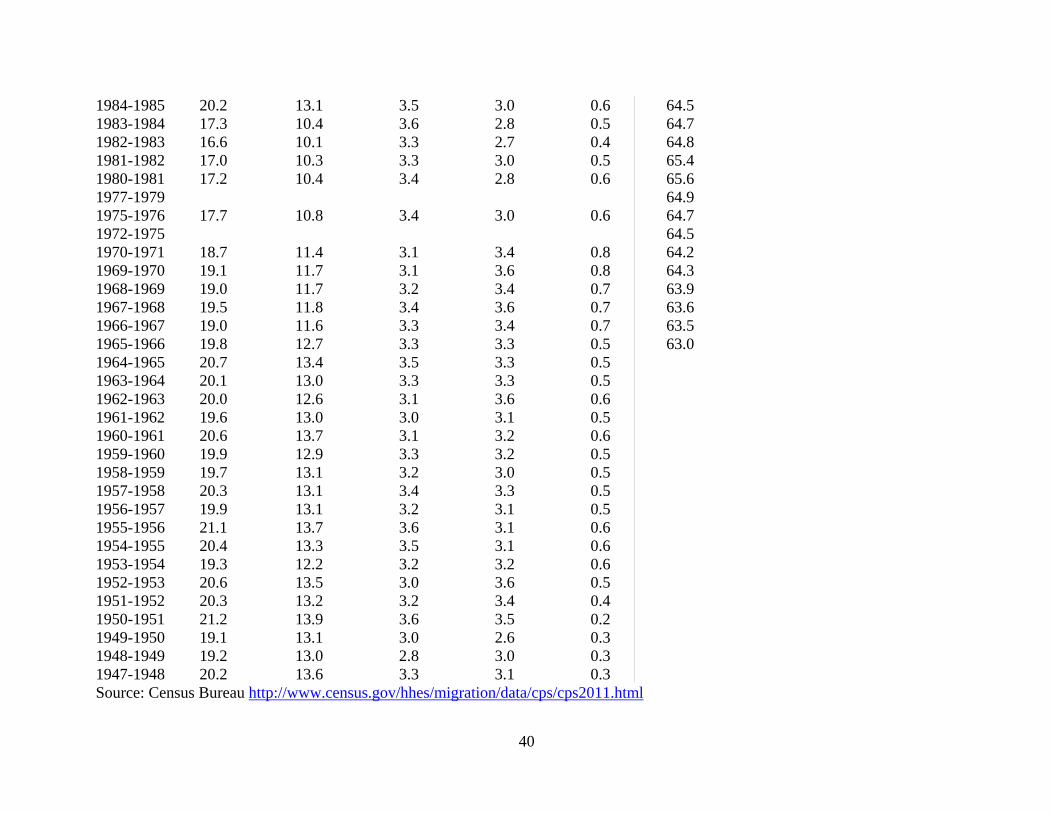
Using US Census data, Table 8 reports for a long run of years -- with some gaps because

of missing data -- the mean values for a variety of different measures of mobility. Five columns

are given. The data in the first column are on the total proportion of citizens moving their place

of residence during the year. In 2010-2011, for example, 11.6% of Americans moved home. In

1947-48, the figure was 20.2%. This much larger number was not because of the closeness of

1947 to the end of the Second World War: until the end of the 1960s the proportion of movers

continued to be approximately 20%. As column 1 of Table 8 shows, from the 1970s to the

2000s there is evidence of a secular downtrend in the “% movers”. Even before the housing

crash of 2008-9, the percentage of Americans moving residence had fallen to approximately

14% per annum.

14

In columns 2 to 5 of Table 8, the figure for total percentage movers is disaggregated. For

2010-2011, for example, the total figure of 11.6% was made up of:

11.6% total movers = 7.7% movers within the county + 2.0% movers within the state +

1.6% movers out of state to another state + 0.4% movers out of the United States itself

and this breakdown gives an arithmetical sense of the huge degree of geographical flows that go

on within a 12 month period. As the identity equation in italics makes clear, there are different

ways to measure ‘mobility’ in the USA. We start analytically with the left-hand side variable,

namely, “% total movers”.

To get a sense of the relationship between the rate of geographical movement and the

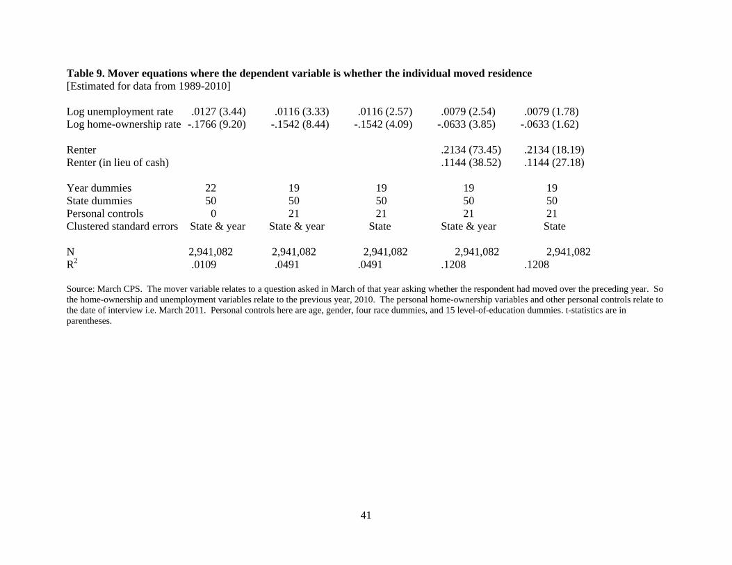
home-ownership rate, Table 9 provides a set of micro-econometric equations. In this case the

dependent variable is a zero-one variable for whether the survey respondent moved home in the

preceding 12 months. In the first column of Table 9, state and year dummies are included, but

the only other independent variables are the state unemployment rate and the home-ownership

rate in the state. As might be expected from standard economic theory, people are more likely to

have moved if there is a high degree of joblessness in their state (the coefficient is 0.0127 with a

t-statistic of 3.44). Moreover, areas with a high level of home-ownership have lower mobility,

ceteris paribus. The coefficient in the first column of Table 9 is -0.1766 with a large t-statistic.

This implies that the rate of movement in a state is nearly 18 percentage points lower in a place

with double the home-ownership rate of another area.

These results are broadly consistent with an earlier study by Hamalainen and Bockerman

(2004) who find that net migration to a region (of Finland) appears to be depressed, ceteris

paribus, by a greater level of home-ownership in that region.

15

The coefficients in column 1 of Table 9 are only marginally influenced by the addition to

the regression equation of a set of personal controls (such as the individual’s age and level of

education). Columns 2 and 3 demonstrate the apparent robustness. The coefficient on the

logarithm of state home-ownership falls in size only slightly to -0.1542. However, as more

variables, and in particular ones for whether the individual is a renter or owner, are added to the

columns of Table 9, the log of the home-ownership rate in the state drops. If standard errors are

clustered at the state level alone, then the variable loses statistical significance. As might be

expected, the variables for the literal housing status of the person are strong. Being a renter is

associated with a much greater chance of being a mover. In the final column of Table 9, that

coefficient is 0.2134. In this equation, the coefficient on the log of home-ownership is -0.0633

with a t-statistic of 1.62.

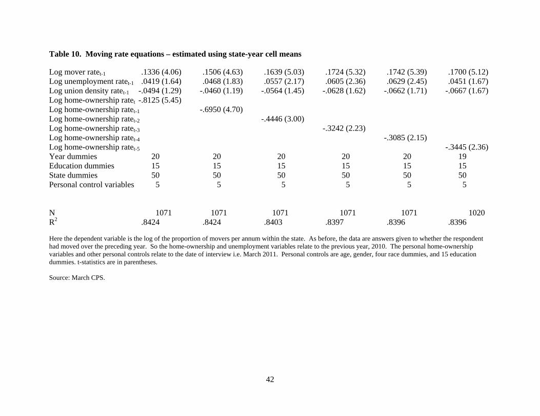
Because mobility can be conceived of more broadly, Table 10 estimates equations

instead for both within-state and out-of-state mobility combined. In this case there is evidence

of a robust negative effect of state home-ownership upon the rate of mobility. The first column

of Table 10 estimates the state-panel equation:

Log Mover Rate in t = f(Log Mover Rate in t-1, Log Unem Rate in t-1, Log Union Density Rate

in t-1, Log Home-ownership Rate in t-1, state dummies, year dummies, personal controls).

There is a smallish but statistically significant degree of auto-regression in the mover

equations of Table 10. The coefficient on the lagged dependent variable enters with a coefficient

of 0.1336. More interestingly, the degree of home-ownership in the state has a substantial effect.

Its coefficient is -0.8125 with a t-statistic greater than 5. As we add longer and longer lags of

16

home-ownership, going from column 1 to column 6 in Table 10, the coefficient drops in size (to

a still-substantial -0.3445) but retains its negative sign and its statistical significance at

conventional cut-off levels.

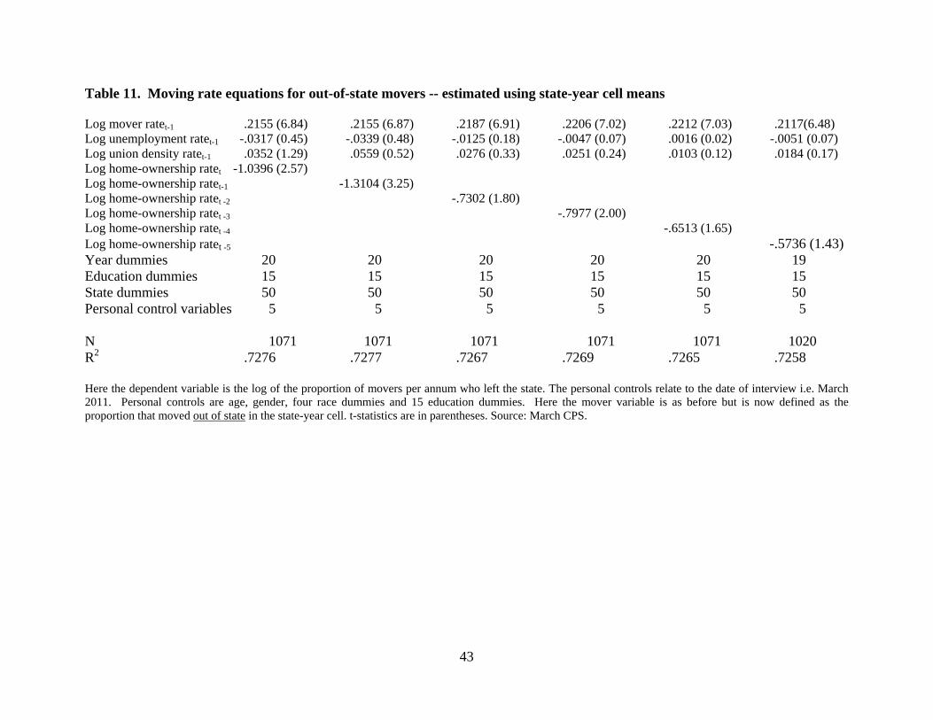
A classic issue in the economics of migration is to what extent workers move long

distances. It is possible to study this within the continental United States by using data on state-

to-state moves. Table 11 presents regression results. It takes as its dependent variable the

proportion of out-of-state movers, which is a subset of the movers examined in Table 9. Some

of the underlying changes in residence may be of a comparatively short distance -- if for

example a New Hampshire worker chooses to relocate just over the state border in Vermont --

but on average they will be larger moves than for the within-state data of Table 10.

In Table 11 our concern is again with whether there is evidence that having a high home-

ownership rate in the state is inimical to mobility. Column 1 of Table 11 estimates a mover-rate

equation in which there is a lagged dependent variable, a state unemployment variable, a state

union density variable, the home-ownership variable, a set of year and state dummies, and

variables for the degree of education and personal characteristics of citizens in the state. In this

and later columns, the lagged dependent variable enters with a well-determined coefficient of

approximately 0.2. The coefficients on the unemployment and union variables are not

statistically different from zero. Home-ownership, however, enters in a statistically significant

way in column 1 of Table 11. At more than unity, its elasticity is large. That number implies

that a doubling of the home-ownership rate would be associated with a halving of the mobility

rate. Column 2 examines the same regression equation but with a one-year lag on the home-

ownership variable. The result is the same and the elasticity now larger. Going to longer lags,

however, pushes down both the coefficient and the degree of statistical significance.

17

It is possible that the links between high home-ownership and later high unemployment

are nothing to do with the degree of labor mobility. If so, what other processes might be at

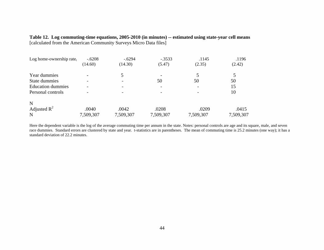
work? To try to probe possible mechanisms, Table 12 examines whether there is a connection

between home-ownership levels in an area and the ease with which individuals can get to their

workplace. Any model with a neoclassical flavor would suggest that the cost of travelling to

work should act as an impediment to the rate of employment (because it raises the opportunity

cost of a job). Table 12 shows that high home-ownership is associated with longer commuting

times, which is consistent with the idea that moving for an owner-occupier is expensive, and that

in consequence the places with high home-ownership will see more workers staying put

physically but working further from their family home. Because roads, in particular, are semi-

public goods in which individuals can create congestion problems for others, this pattern in the

data is consistent with the existence of un-priced externalities. The elasticity in the final column

of Table 12 is approximately 0.12.

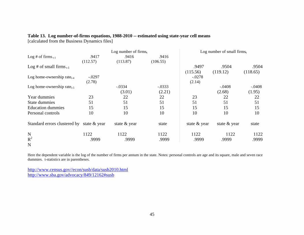
Table 13 and Table 14 turn to the possible concern that -- for zoning or NIMBY or other

reasons -- a high degree of home-ownership in an area might be associated with a lower degree

of tolerance for new businesses. Table 13 estimates regressions equations in which the

dependent variable is the number of registered firms in the state. State home-ownership enters

negatively in these equations with a coefficient of approximately -0.03 and a t-statistic greater

than 2. The right-hand segment of Table 13 reports the same equations for small firms. Once

again, the size of these estimated effects in the regression equations seem to be economically and

not just statistically significant. The implied long-run elasticities from home-ownership on to

business formation are large.

18

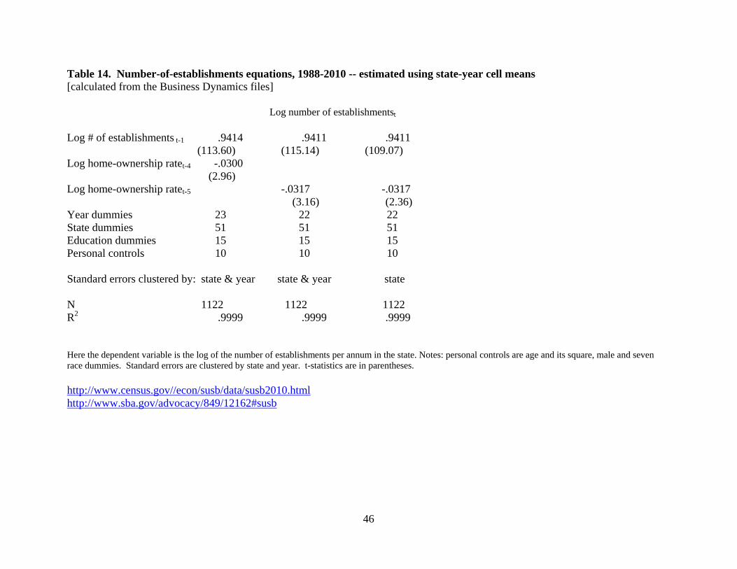
Similar patterns emerge using data on U.S. establishments rather than on firms. The

results are given in the state-panel equations of Table 14, where the lagged dependent variable

has a large coefficient, and the logarithm of the home-ownership rate in the state enters with a

coefficient of approximately -0.03. Although more research will be required on this topic, and

the detailed mechanisms are currently unknown, these findings are consistent with the view that

high home-ownership levels may be inimical to business formation rates.

5. Conclusions

The results in this paper are consistent with the view that high home-ownership impairs

the vitality of the labor market and slowly grinds out greater rates of joblessness. Given the

emphasis that most western governments put on the promotion of home-ownership (one

exception is Switzerland, which taxes home-owners’ imputed rents), it is important that other

researchers check and probe these results. Taken at face value, our findings should be worrying

for policy-makers. A possible reason why these patterns have attracted so little notice from both

researchers and the public is that the time lags are long. High levels of home-ownership do not

destroy jobs this year; they tend to do so, on our estimates, the year after next. Unless these long

linkages are studied, the consequences of high levels of home-ownership are not easy to see.

What mechanism lies behind the findings? It is not possible to be certain. Our main

contribution should be seen as a statistical one -- as documenting patterns of potential interest to

economists and social scientists, and perhaps especially to labor economists, macroeconomists,

economic geographers, and urban economists. Nevertheless, we have made an attempt to look

below the reduced-form link between current home-ownership and later joblessness. In doing

so, we have found evidence that high home-ownership in a U.S. state is associated with

(i) lower labor mobility,

19

(ii) longer commutes, and

(iii) fewer new firms and establishments.

It should be emphasized that this is after we have controlled for state fixed effects and a range of

possible confounding variables. Our results are consistent with the recent conclusions of a

European study done independently by Laamanen (2013). His study has a number of stronger

methodological features than were available to us.

We have estimated equations using micro data from the United States from the 1980s to

the present day. There are four main conclusions. First, rises in a US state’s home-ownership

rate are associated with later rises in joblessness in that state. The long run elasticity is estimated

to lie between 1 and 2. This is strikingly large. It suggests that a doubling of home-ownership

in a state would be associated in the steady state with more than a doubling of the unemployment

rate. Second, after controlling for state fixed-effects, we show that areas with higher ownership

have lower mobility. The long-run elasticity is approximately -0.3. Third, high home-

ownership areas have longer commute-to-work times, which can be expected in those areas to

raise costs for employers and employees. The long-run elasticity is approximately -0.1. Fourth,

high home-ownership areas have lower rates of business formation. It is conceivable -- we are

not able to offer proof -- that this may be due to zoning or NIMBY effects. That conjecture

deserves scrutiny in future research.

It is important to emphasize that our study does not claim that home owners are

unemployed more than renters (very probably they are not). Nor is it an attempt to build on the

idea that home owners are less mobile than renters (though they probably are). Instead, because

the estimates in Tables 7 and 9 of the paper control for whether individuals are themselves

20

renters or owners, the patterns documented in the paper are consistent with the possibility that

the housing market can generate important negative externalities upon the labor market.

Our analysis has a number of important weaknesses. Unlike Laamanen (2013), we are

unable to assess the effect of exogenous changes in the structure of the housing market. We

have had to rely, instead, upon an examination of the lagged pattern of unemployment observed

a number of years after a movement in a state’s rate of home-ownership. Thus our study adopts

the so-called ‘prospective study’ format that is common in medical science and epidemiology.

This is potentially a weakness and means that some underlying omitted variable, or causal force,

might be responsible for the link between Ht and Ut+n. That would not make the patterns in this

paper uninteresting ones, but it would mean that a key variable is missing from the analysis.

Another lacuna in our study is a detailed account of the processes by which the housing market

affects the equilibrium rates of unemployment and employment. It may be that the effect of high

home-ownership comes partly from some engendered reduction in the rate of labor mobility

within a geographical area. However, we are doubtful that this works in a classical way through

a lower amount of state-to-state migration.14 Finally, unlike McCormick (1983), we have been

unable to distinguish between those owners who are currently paying a mortgage and those who

own their home outright.

Economists currently lack a full understanding of the interplay between the housing and

labor markets. We believe these issues demand the profession’s attention.

14 There is evidence -- using a variety of statistical methods -- that Adam Smith’s compensating differentials theory of equal utility across geographical space successfully fits the data for the states of the USA (see Roback, 1982, for example; or recently Herz and Van Rens, 2012, on the inability of mismatch to explain recent US experience; or in a different way the work of Oswald and Wu, 2010). Consistent with this, new work by Modestino and Dennett (2013) finds little evidence that house-lock contributes to the pattern of US unemployment.

21

22

References Battu, H., Ma, A., and Phimister, E. 2008. Housing tenure, job mobility and unemployment in

the UK. Economic Journal, 118, 311-328. Bell, D., & Blanchflower, D.G. 2010. UK unemployment in the great recession. National

Institute Economic Review, London, October. Blanchard, O., and Katz, L.F. 1992. Regional evolutions. Brookings Papers on Economic

Activity, 1, 1-77. Blanchflower, D.G., and Oswald, A.J. 1994. The wage curve. MIT Press: Cambridge MA. Coulson, N.E., and Fisher, L.M. 2002. Tenure choice and labor market outcomes. Housing

Studies, 17, 35-49. Coulson, N.E., and Fisher, L.M. 2009. Housing tenure and labor market impacts: The search

goes on. Journal of Urban Economics, 65, 252-264. Dickens, W.T., and Triest, R.K. 2012. Potential effects of the Great Recession on the US labor

market. BE Journal of Macroeconomics, 12, article number 8. DiTella, R., MacCulloch, R.J., and Oswald, A.J. 2003. The macroeconomics of happiness.

Review of Economics and Statistics, 85, 809-827. Dohmen, T.J. 2005. Housing, mobility and unemployment. Regional Science and Urban

Economics, 35, 305-325. Dujardin, C., and Goffette-Nagot, F. 2009. Does public housing occupancy increase

unemployment? Journal of Economic Geography, 9, 823-851. Ferreira, F., Gyourko, J., and Tracy J. 2010. Housing busts and household mobility. Journal of

Urban Economics, 68, 34-45. Fischel, W.A. 2004. An economic history of zoning and a cure for its exclusionary effects.

Urban Studies, 41, 317-340. Green, R.K., and Hendershott, P.H. 2001. Home-ownership and unemployment in the US.

Urban Studies, 38, 1509-1520. Hamalainen, K. and Bockerman, P. 2004. Regional labour market dynamics, housing, and

migration. Journal of Regional Science, 44, 543-568. Head, A., and Lloyd-Ellis, H. 2012. Housing liquidity, mobility, and the labor market. Review of

Economic Studies, 79, 1559-1589. Herz, B., and Van Rens, T. 2012. Accounting for mismatch unemployment. Working paper,

University of Warwick. Hughes, G., and McCormick, B. 1981. Do council housing policies reduce migration between

regions? Economic Journal, 91, 919-937. Laamanen, J-P. 2013. Home ownership and the labour market: Evidence from rental housing

market deregulation. Tampere Economic Working Paper, No. 89, University of Tampere, Finland. Downloadable at http://tampub.uta.fi/handle/10024/68116

Layard, R., Nickell, S.J., and Jackman, R. 1991. Unemployment: Macroeconomic performance and the labor market. Oxford University Press: Oxford.

Linn, M.W., Sandifer, R., and Stein, S. 1985. Effects of unemployment on mental and physical health. American Journal of Public Health, 75, 502-506.

McCormick, B. 1983. Housing and unemployment in Great Britain. Oxford Economic Papers, 35(S), 283-305.

Modestino, A.S., and Dennett, J. 2013. Are American homeowners locked into their houses? The impact of housing conditions on state-to-state migration. Regional Science and Urban

23

Economics, 43, 322-337. Mortensen, D.T., and Pissarides, C.A. 1994. Job creation and job destruction in the theory of

unemployment. Review of Economic Studies, 61, 397-415. Munch, J.R., Rosholm, M., and Svarer, M. 2006. Are home owners really more unemployed?

Economic Journal, 116, 991-1013. Murphy, G.C., and Athanasou, J.A. 1999. The effect of unemployment on mental health. Journal

of Occupational and Organizational Psychology, 72, 83-99. OECD. 1994. The Jobs Study, Paris, France. Oswald, A.J. 1996. A conjecture on the explanation for high unemployment in the industrialized

nations: Part 1. University of Warwick Economic Research Paper 475. Oswald, A.J. 1997. Thoughts on NAIRU. Journal of Economic Perspectives, 11, 227-228. Oswald, A.J. 1999. The housing market and Europe’s unemployment: A non-technical paper.

Unpublished, University of Warwick. Oswald, A.J., and Wu, S. 2010. Objective confirmation of subjective measures of human well-

being: Evidence from the USA. Science, 327, 576-579. Paul, K.I., and Moser, K. 2009. Unemployment impairs mental health: Meta-analyses. Journal of

Vocational Behavior, 74, 264-282. Petrongolo, B., and Pissarides, C.A. 2001. Looking into the black box: A survey of the matching

function. Journal of Economic Literature, 39, 390-431. Pigou, A. 1914. Unemployment. Holt: New York. Powdthavee, N. 2010. The happiness equation. Icon Books: Duxford. Roback, J. 1982. Wages, rents, and the quality of life. Journal of Political Economy, 90, 1257-

1278. Rouwendal, J., and Nijkamp, P. 2010. Home-ownership and labor market behaviour:

Interpreting the evidence, Environment and Planning A. 42, 419-433. Serafinelli, M. 2012. Good firms, worker flows, and productivity. Working paper, UC Berkeley. Smith, T.E., and Zenou, Y. 2003. Spatial mismatch, search effort, and urban spatial structure,

Journal of Urban Economics. 54, 129-156. Valletta, R. 2012. House-lock and structural unemployment. Working paper 2012-25, Federal

Reserve Bank of San Francisco. Van Leuvensteijn, M., and Koning, P. 2004. The effect of home-ownership on labor mobility in

the Netherlands. Journal of Urban Economics, 55, 580-596. Zabel, J.E. 2012. Migration, housing market, and labor market responses to employment shocks.

Journal of Urban Economics, 72, 267-284.

24

25

The States of the USA: Changes over Half a Century

26

Chart 3. The Impulse Response Function in Log Unemployment after a One Unit Rise in Home Ownership

This uses the representative equation:

lnun(t) = .784*lnun(t-1) + .4302 home(t-5)

27

Table 1. Historical home-ownership rates (%) in the US: By decade from 2010 back to 1900

2010 2000 1990 1980 1970 1960 1950 1940 1930 1920 1910 1900 United States 65.1% 66.2 64.2 64.4 62.9 61.9 55.0 43.6 47.8 45.6 45.9 46.5 Alabama 69.7 72.5 70.5 70.1 66.7 59.7 49.4 33.6 34.2 35.0 35.1 34.4 Alaska 63.1 62.5 56.1 58.3 50.3 48.3 54.5 NA NA NA NA NA Arizona 66.0 68.0 64.2 68.3 65.3 63.9 56.4 47.9 44.8 42.8 49.2 57.5 Arkansas 67.0 69.4 69.6 70.5 66.7 61.4 54.5 39.7 40.1 45.1 46.6 47.7 California 55.9 56.9 55.6 55.9 54.9 58.4 54.3 43.4 46.1 43.7 49.5 46.3 Colorado 65.5 67.3 62.2 64.5 63.4 63.8 58.1 46.3 50.7 51.6 51.5 46.6 Connecticut 67.5 66.8 65.6 63.9 62.5 61.9 51.1 40.5 44.5 37.6 37.3 39.0 Delaware 72.1 72.3 70.2 69.1 68.0 66.9 58.9 47.1 52.1 44.7 40.7 36.3 DC 42.0 40.8 38.9 35.5 28.2 30.0 32.3 29.9 38.6 30.3 25.2 24.0 Florida 67.4 70.1 67.2 68.3 68.6 67.5 57.6 43.6 42.0 42.5 44.2 46.8 Georgia 65.7 67.5 64.9 65.0 61.1 56.2 46.5 30.8 30.6 30.9 30.5 30.6 Hawaii 57.7 56.5 53.9 51.7 46.9 41.1 33.0 NA NA NA NA NA Idaho 69.9 72.4 70.1 72.0 70.1 70.5 65.5 57.9 57.0 60.9 68.1 71.6 Illinois 67.5 67.3 64.2 62.6 59.4 57.8 50.1 40.3 46.5 43.8 44.1 45.0 Indiana 69.9 71.4 70.2 71.7 71.7 71.1 65.5 53.1 57.3 54.8 54.8 56.1 Iowa 72.1 72.3 70.0 71.8 71.7 69.1 63.4 51.5 54.7 58.1 58.4 60.5 Kansas 67.8 69.2 67.9 70.2 69.1 68.9 63.9 51.0 56.0 56.9 59.1 59.1 Kentucky 68.7 70.8 69.6 70.0 66.9 64.3 58.7 48.0 51.3 51.6 51.6 51.5 Louisiana 67.2 67.9 65.9 65.5 63.1 59.0 50.3 36.9 35.0 33.7 32.2 31.4 Maine 71.3 71.6 70.5 70.9 70.1 66.5 62.8 57.3 61.7 59.6 62.5 64.8 Maryland 67.5 67.7 65.0 62.0 58.8 64.5 56.3 47.4 55.2 49.9 44.0 40.0 Massachusetts 62.3 61.7 59.3 57.5 57.5 55.9 47.9 38.1 43.5 34.8 33.1 35.0 Michigan 72.1 73.8 71.0 72.7 74.4 74.4 67.5 55.4 59.0 58.9 61.7 62.3 Minnesota 73.0 74.6 71.8 71.7 71.5 72.1 66.4 55.2 58.9 60.7 61.9 63.5 Mississippi 69.6 72.3 71.5 71.0 66.3 57.7 47.8 33.3 32.5 34.0 34.0 34.5 Missouri 68.8 70.3 68.8 69.6 67.2 64.3 57.7 44.3 49.9 49.5 51.1 50.9 Montana 68.0 69.1 67.3 68.6 65.7 64.0 60.3 52.0 54.5 60.5 60.0 56.6 Nebraska 67.2 67.4 66.5 68.4 66.4 64.8 60.6 47.1 54.3 57.4 59.1 56.8 Nevada 58.8 60.9 54.8 59.6 58.5 56.3 48.7 46.1 47.1 47.6 53.4 66.2

28

New Hampshire 71.0 69.7 68.2 67.6 68.2 65.1 58.1 51.7 55.0 49.8 51.2 53.9 New Jersey 65.4 65.6 64.9 62.0 60.9 61.3 53.1 39.4 48.4 38.3 35.0 34.3 New Mexico 68.5 70.0 67.4 68.1 66.4 65.3 58.8 57.3 57.4 59.4 70.6 68.5 New York 53.3 53.0 52.2 48.6 47.3 44.8 37.9 30.3 37.1 30.7 31.0 33.2 North Carolina 66.7 69.4 68.0 68.4 65.4 60.1 53.3 42.4 44.5 47.4 47.3 46.6 North Dakota 65.4 66.6 65.6 68.7 68.4 68.4 66.2 49.8 58.6 65.3 75.7 80.0 Ohio 67.6 69.1 67.5 68.4 67.7 67.4 61.1 50.0 54.4 51.6 51.3 52.5 Oklahoma 67.2 68.4 68.1 70.7 69.2 67.0 60.0 42.8 41.3 45.5 45.4 54.2 Oregon 62.2 64.3 63.1 65.1 66.1 69.3 65.3 55.4 59.1 54.8 60.1 58.7 Pennsylvania 69.6 71.3 70.6 69.9 68.8 68.3 59.7 45.9 54.4 45.2 41.6 41.2 Rhode Island 60.7 60.0 59.5 58.8 57.9 54.5 45.3 37.4 41.2 31.1 28.3 28.6 South Carolina 69.3 72.2 69.8 70.2 66.1 57.3 45.1 30.6 30.9 32.2 30.8 30.6 South Dakota 68.1 68.2 66.1 69.3 69.6 67.2 62.2 45.0 53.1 61.5 68.2 71.2 Tennessee 68.2 69.9 68.0 68.6 66.7 63.7 56.5 44.1 46.2 47.7 47.0 46.3 Texas 63.7 63.8 60.9 64.3 64.7 64.8 56.7 42.8 41.7 42.8 45.1 46.5 Utah 70.4 71.5 68.1 70.7 69.3 71.7 65.3 61.1 60.9 60.0 64.8 67.8 Vermont 70.7 70.6 69.0 68.7 69.1 66.0 61.3 55.9 59.8 57.5 58.5 60.4 Virginia 67.2 68.1 66.3 65.6 62.0 61.3 55.1 48.9 52.4 51.1 51.5 48.8 Washington 63.9 64.6 62.6 65.6 66.8 68.5 65.0 57.0 59.4 54.7 57.3 54.5 West Virginia 73.4 75.2 74.1 73.6 68.9 64.3 55.0 43.7 45.9 46.8 49.5 54.6 Wisconsin 68.1 68.4 66.7 68.2 69.1 68.6 63.5 54.4 63.2 63.6 64.6 66.4 Wyoming 69.2 70.0 67.8 69.2 66.4 62.2 54.0 48.6 48.3 51.9 54.5 55.2 Source: US Census Bureau

29

Table 2a. Recent annual home-ownership rates in the US: 2000-2010

2000 2001 2002 2003 2004 2005 2006 2007 2008 2009 2010 United States 67.4% 67.8 67.9 68.3 69.0 68.9 68.8 68.1 67.8 67.4 66.9 Alabama 73.2 73.2 73.7 76.2 78.0 76.6 74.2 73.3 73.0 74.1 73.2 Alaska 66.4 65.3 67.1 70.0 67.2 66.0 67.2 66.6 66.4 66.8 65.7 Arizona 68.0 68.1 65.6 67.0 68.7 71.1 71.6 70.4 69.1 68.9 66.6 Arkansas 68.9 71.2 70.3 69.6 69.1 69.2 70.8 69.5 68.9 68.5 67.9 California 57.1 58.2 57.7 58.9 59.7 59.7 60.2 58.3 57.5 57.0 56.1 Colorado 68.3 68.5 68.9 71.3 71.1 71.0 70.1 70.2 69.0 68.4 68.5 Connecticut 70.0 71.8 71.5 73.0 71.7 70.5 71.1 70.3 70.7 70.5 70.8 Delaware 72.0 75.4 75.6 77.2 77.3 75.8 76.8 76.8 76.2 76.5 74.7 DC 41.9 42.7 44.1 43.0 45.6 45.8 45.9 47.2 44.1 44.9 45.6 Florida 68.4 69.2 68.7 69.5 72.2 72.4 72.4 71.8 71.1 70.9 69.3 Georgia 69.8 70.1 71.8 71.4 70.9 67.9 68.5 67.6 68.2 67.4 67.1 Hawaii' 55.2 55.5 57.9 58.3 60.6 59.8 59.9 60.1 59.1 59.5 56.1 Idaho 70.5 71.7 73.0 74.4 73.7 74.2 75.1 74.5 75.0 75.5 72.4 Illinois 67.9 69.4 70.1 70.7 72.7 70.9 70.4 69.4 68.9 69.1 68.8 Indiana 74.9 75.3 75.1 74.4 75.8 75.0 74.2 73.8 74.4 72.0 71.2 Iowa 75.2 76.6 73.9 73.4 73.2 73.9 74.0 73.7 74.0 72.4 71.1 Kansas 69.3 70.4 70.3 70.3 69.9 69.5 70.0 69.4 68.8 67.4 67.4 Kentucky 73.4 73.9 73.7 74.4 73.3 71.6 71.7 72.9 72.8 71.2 70.3 Louisiana 68.1 67.1 67.4 67.5 70.6 72.5 71.3 71.5 73.5 71.9 70.4 Maine 76.5 75.5 74.0 73.7 74.7 73.9 75.3 74.3 73.9 74.0 73.8 Maryland 69.9 70.7 72.0 71.6 72.1 71.2 72.6 71.7 70.6 69.6 68.9 Massachusetts 59.9 60.6 62.6 64.3 63.8 63.4 65.2 64.3 65.7 65.1 65.3 Michigan 77.2 77.1 76.0 75.6 77.1 76.4 77.4 76.4 75.9 74.5 74.5 Minnesota 76.1 76.1 77.3 77.2 76.4 76.5 75.6 73.5 73.1 72.9 72.6 Mississippi 75.2 74.5 74.9 73.4 74.0 78.8 76.2 74.0 75.4 75.5 74.8 Missouri 74.2 74.0 74.8 74.0 72.4 72.3 71.9 70.4 71.4 72.0 71.2 Montana 70.2 68.3 69.4 71.5 72.4 70.4 69.5 67.3 70.3 70.7 68.1 Nebraska 70.2 70.1 68.5 69.5 71.2 70.2 67.6 68.2 69.6 70.2 70.4 Nevada 64.0 64.6 65.3 64.8 65.7 63.4 65.7 63.3 63.6 62.4 59.7

30

New Hampshire 69.2 68.4 69.5 74.4 73.3 74.0 74.2 73.8 75.0 76.0 74.9 New Jersey 66.2 66.5 66.9 66.9 68.8 70.1 69.0 68.3 67.3 65.9 66.5 New Mexico 73.7 70.8 70.0 70.3 71.5 71.4 72.0 71.5 70.4 69.1 68.6 New York 53.4 53.9 54.8 54.3 54.8 55.9 55.7 55.9 55.0 54.4 54.5 North Carolina 71.1 71.3 70.0 70.0 69.8 70.9 70.2 70.3 69.4 70.1 69.5 North Dakota 70.7 71.0 69.4 68.7 70.0 68.5 68.3 66.0 66.6 65.7 67.1 Ohio 71.3 71.2 72.1 72.8 73.1 73.3 72.1 71.4 70.8 69.7 69.7 Oklahoma 72.7 71.5 69.6 69.1 71.1 72.9 71.6 70.3 70.4 69.6 69.2 Oregon 65.3 65.8 66.2 68.0 69.0 68.2 68.1 65.7 66.2 68.2 66.3 Pennsylvania 74.7 74.3 74.0 73.7 74.9 73.3 73.2 72.9 72.6 72.2 72.2 Rhode Island 61.5 60.1 59.4 59.9 61.5 63.1 64.6 64.9 64.5 62.9 62.8 South Carolina 76.5 76.1 77.5 75.0 76.2 73.9 74.2 74.1 73.9 74.4 74.8 South Dakota 71.2 71.5 71.5 70.9 68.5 68.4 70.6 70.4 70.4 69.6 70.6 Tennessee 70.9 69.7 70.3 70.8 71.6 72.4 71.3 70.2 71.7 71.1 71.0 Texas 63.8 63.9 63.4 64.5 65.5 65.9 66.0 66.0 65.5 65.4 65.3 Utah 72.7 72.4 72.8 73.4 74.9 73.9 73.5 74.9 76.2 74.1 72.5 Vermont 68.7 69.8 70.3 71.4 72.0 74.2 74.0 73.7 72.8 74.3 73.6 Virginia 73.9 75.1 74.4 75.0 73.4 71.2 71.1 71.5 70.6 69.7 68.7 Washington 63.6 66.4 66.9 65.9 66.0 67.6 66.7 66.8 66.2 65.5 64.4 West Virginia 75.9 76.4 77.2 78.1 80.3 81.3 78.4 77.6 77.8 78.7 79.0 Wisconsin 71.8 72.3 72.2 72.8 73.3 71.1 70.2 70.5 70.4 70.4 71.0 Wyoming 71.0 73.5 73.0 72.9 72.8 72.8 73.7 73.2 73.3 73.8 73.4 Source (here and in the next table): Current Population Survey

31

Table 2b. Annual home-ownership rates in the 1980s and 1990s in the US

1984 1985 1986 1987 1988 1989 1990 1991 1992 1993 1994 1995 1996 1997 1998 1999 USA 64.5% 63.9 63.8 64.0 63.8 63.9 63.9 64.1 64.1 64.0 64.0 64.7 65.4 65.7 66.3 66.8 Alabama 73.7 70.4 70.3 67.9 66.5 67.6 68.4 69.9 70.3 70.2 68.5 70.1 71.0 71.3 72.9 74.8 Alaska 57.6 61.2 61.5 59.7 57.0 58.7 58.4 57.1 55.5 55.4 58.8 60.9 62.9 67.2 66.3 66.4 Arizona 65.2 64.7 62.5 63.3 66.1 63.9 64.5 66.3 69.3 69.1 67.7 62.9 62.0 63.0 64.3 66.3 Arkansas 65.9 66.6 67.5 68.1 67.0 66.3 67.8 68.6 70.3 70.5 68.1 67.2 66.6 66.7 66.7 65.6 California 53.7 54.2 53.8 54.3 54.4 53.6 53.8 54.5 55.3 56.0 55.5 55.4 55.0 55.7 56.0 55.7 Colorado 64.7 63.6 63.7 61.8 60.1 58.6 59.0 59.8 60.9 61.8 62.9 64.6 64.5 64.1 65.2 68.1 Connecticut 67.8 69.0 68.1 67.0 66.5 66.4 67.9 65.5 66.1 64.5 63.8 68.2 69.0 68.1 69.3 69.1 Delaware 70.4 70.3 71.0 71.1 70.1 68.7 67.7 70.2 73.8 74.1 70.5 71.7 71.5 69.2 71.0 71.6 DC 37.3 37.4 34.6 35.8 37.5 38.7 36.4 35.1 35.0 35.7 37.8 39.2 40.4 42.5 40.3 40.0 Florida 66.5 67.2 66.5 66.3 64.9 64.4 65.1 66.1 66.0 65.5 65.7 66.6 67.1 66.9 66.9 67.6 Georgia 63.6 62.7 62.4 63.9 64.8 64.7 64.3 65.7 66.9 66.5 63.4 66.6 69.3 70.9 71.2 71.3 Hawaii 50.7 51.0 50.9 50.7 53.2 54.7 55.5 55.2 53.8 52.8 52.3 50.2 50.6 50.2 52.8 56.6 Idaho 69.7 71.0 69.8 71.6 71.5 70.2 69.4 68.4 70.3 72.1 70.7 72.0 71.4 72.3 72.6 70.3 Illinois 62.4 60.6 60.9 61.0 61.4 61.9 63.0 63.0 62.4 61.8 64.2 66.4 68.2 68.1 68.0 67.1 Indiana 69.9 67.6 67.6 69.1 68.3 68.2 67.0 66.1 67.6 68.7 68.4 71.0 74.2 74.1 72.6 72.9 Iowa 71.3 69.9 69.2 67.7 68.3 69.6 70.7 68.4 66.3 68.2 70.1 71.4 72.8 72.7 72.1 73.9 Kansas 72.7 68.3 66.4 67.9 68.6 68.1 69.0 69.7 69.8 68.9 69.0 67.5 67.5 66.5 66.7 67.5 Kentucky 70.2 68.5 68.1 67.6 65.4 64.9 65.8 67.2 69.0 68.8 70.6 71.2 73.2 75.0 75.1 73.9 Louisiana 70.1 70.2 70.4 71.0 68.5 66.3 67.8 68.9 66.7 65.4 65.8 65.3 64.9 66.4 66.6 66.8 Maine 74.1 73.7 74.0 73.2 72.2 73.6 74.2 72.0 72.0 71.9 72.6 76.7 76.5 74.9 74.6 77.4 Maryland 67.8 65.6 62.8 62.7 63.5 65.5 64.9 63.8 64.8 65.5 64.1 65.8 66.9 70.5 68.7 69.6 Massachusetts 61.7 60.5 60.3 60.6 60.0 58.9 58.6 60.2 61.8 60.7 60.6 60.2 61.7 62.3 61.3 60.3 Michigan 72.7 70.7 70.9 71.7 72.5 73.2 72.3 70.6 70.6 72.3 72.0 72.2 73.3 73.3 74.4 76.5 Minnesota 72.6 70.0 68.0 68.9 69.1 68.3 68.0 68.9 66.7 65.8 68.9 73.3 75.4 75.4 75.4 76.1 Mississippi 72.3 69.6 70.4 72.5 73.7 72.2 69.4 71.8 70.4 69.7 69.2 71.1 73.0 73.7 75.1 74.9 Missouri 69.5 69.2 67.8 66.1 64.8 63.7 64.0 64.2 65.2 66.4 68.4 69.4 70.2 70.5 70.7 72.9 Montana 66.4 66.5 64.4 65.0 65.4 67.9 69.1 69.6 69.9 69.7 68.8 68.7 68.6 67.5 68.6 70.6 Nebraska 69.3 68.5 68.3 66.8 66.6 67.2 67.3 67.5 68.4 67.7 68.0 67.1 66.8 66.7 69.9 70.9 Nevada 58.9 57.0 54.5 54.1 54.3 54.3 55.8 55.8 55.1 55.8 55.8 58.6 61.1 61.2 61.4 63.7

32

N. Hampshire 67.1 65.5 64.8 66.4 67.9 67.0 65.0 66.8 66.6 65.4 65.1 66.0 65.0 66.8 69.6 70.2 New Jersey 63.4 62.3 63.3 64.0 64.8 65.7 65.0 64.8 64.6 64.5 64.1 64.9 64.6 63.1 63.1 64.5 New Mexico 68.0 68.2 67.8 67.2 65.4 65.5 68.6 69.5 70.5 69.1 66.8 67.0 67.1 69.6 71.3 72.6 New York 51.1 50.3 51.3 52.0 50.7 52.3 53.3 52.6 53.3 52.8 52.5 52.7 52.7 52.6 52.8 52.8 N Carolina 68.8 68.0 68.2 68.4 68.3 69.4 69.0 69.3 68.6 68.8 68.7 70.1 70.4 70.2 71.3 71.7 N Dakota 70.1 69.9 69.2 68.9 67.7 67.1 67.2 65.4 63.7 62.7 63.3 67.3 68.2 68.1 68.0 70.1 Ohio 67.7 67.9 68.2 68.6 69.6 69.6 68.7 68.7 69.1 68.5 67.4 67.9 69.2 69.0 70.7 70.7 Oklahoma 71.0 70.5 69.7 70.9 72.1 71.4 70.3 69.2 68.9 70.3 68.5 69.8 68.4 68.5 69.7 71.5 Oregon 61.9 61.5 63.9 64.6 64.0 63.4 64.4 65.2 64.3 63.8 63.9 63.2 63.1 61.0 63.4 64.3 Pennsylvania 71.1 71.6 72.3 71.8 72.1 72.8 73.8 74.0 73.1 72.0 71.8 71.5 71.7 73.3 73.9 75.2 Rhode Island 60.9 61.4 62.2 60.4 62.0 61.2 58.5 58.2 56.8 57.6 56.5 57.9 56.6 58.7 59.8 60.6 S Carolina 69.1 72.0 70.3 72.8 73.8 71.0 71.4 73.1 71.0 71.1 72.0 71.3 72.9 74.1 76.6 77.1 S Dakota 69.6 67.6 65.9 66.8 66.4 65.8 66.2 66.1 66.5 65.6 66.4 67.5 67.8 67.6 67.3 70.7 Tennessee 67.6 67.6 67.4 67.2 66.9 67.3 68.3 68.0 67.4 64.1 65.2 67.0 68.8 70.2 71.3 71.9 Texas 62.5 60.5 61.0 61.1 59.9 61.0 59.7 59.0 58.3 58.7 59.7 61.4 61.8 61.5 62.5 62.9 Utah 69.9 71.5 68.0 69.0 70.2 70.4 70.1 70.7 70.0 68.9 69.3 71.5 72.7 72.5 73.7 74.7 Vermont 66.9 69.5 69.8 70.5 68.7 69.7 72.6 70.8 70.8 68.5 69.4 70.4 70.3 69.1 69.1 69.1 Virginia 68.3 68.5 68.2 69.0 69.8 70.2 69.8 68.9 67.8 68.5 69.3 68.1 68.5 68.4 69.4 71.2 Washington 65.7 66.8 65.1 64.4 64.2 64.2 61.8 61.8 62.5 63.1 62.4 61.6 63.1 62.9 64.9 64.8 W Virginia 72.0 75.9 76.4 72.5 73.2 74.8 72.0 72.4 73.3 73.3 73.7 73.1 74.3 74.6 74.8 74.8 Wisconsin 65.2 63.8 66.5 68.2 68.0 69.3 68.3 68.9 69.4 65.7 64.2 67.5 68.2 68.3 70.1 70.9 Wyoming 68.8 73.2 72.0 68.9 67.8 69.6 68.9 68.7 67.9 67.1 65.8 69.0 68.0 67.6 70.0 69.8

33

Table 3. Unemployment equations without a lagged dependent variable -- estimated using state-year cell means [calculated from the Merged Outgoing Rotation Group (MORG) files of the US Current Population Survey, 1985-2011] 1985-2011 1986-2011 1987-2011 1988-2011 1989-2011 1989-2011 Log home-ownership rate t-1-.3282 (2.09) -.8309 (3.39)

Log home-ownership rate t-2 .0031 (0.02) .2540 (0.78) Log home-ownership rate t-3 .2083 (1.29) .0012 (0.00)

Log home-ownership rate t-4 .4588 (2.87) -.1520 (0.48)

Log home-ownership rate t-5 .8060 (5.18) 1.0216 (4.40)

Union density -.4232 (1.08) -.5939 (1.47) -.7233 (0.47) -.8038 (1.99) -.1693 (0.70) -.6592 (1.66) Year dummies 25 24 23 22 21 21 State dummies 50 50 50 50 50 50 Education dummies 18 18 18 18 18 18 Personal controls 4 4 4 4 4 4 N 1377 1326 1275 1224 1173 1173 Adjusted R2 .7831 .7792 .7822 .7958 .8151 .8175 Notes: The dependent variable in this table is the log of the state unemployment rate in year t. The personal controls here are age, gender, and two race dummies. t-statistics are in parentheses.

34

Table 4. Unemployment equations with a lagged dependent variable -- estimated using state-year cell means [calculated from the Merged Outgoing Rotation Group (MORG) files of the US Current Population Survey, 1985-2011] 1985-2011 1986-2011 1987-2011 1988-2011 1989-2011 1989-2011 Log unemployment ratet-1 .8482 (50.67) .8536 (50.86) .8442 (51.37) .8173 (49.08) .7840 (45.77) .7860 (45.24) Log home-ownership rate t-1 .2488 (2.73) -.1460 (1.01)

Log home-ownership rate t-2 .3359 (3.69) .3303 (1.73) Log home-ownership rate t-3 .2927 (3.26) -.0837 (0.44)

Log home-ownership rate t-4 .3429 (3.79) -.0171 (0.09)

Log home-ownership rate t-5 .4302 (4.47) .4081 (2.97)

Union density -.1619 (0.71) -.1041 (0.61) -.1066 (0.47) -.1109 (0.48) -.1693 (0.70) -.1402 (0.60) Year dummies 25 24 23 22 21 21 State dummies 50 50 50 50 50 50 Education dummies 18 18 18 18 18 18 Personal controls 4 4 4 4 4 4 N 1377 1326 1275 1224 1173 1173 Adjusted R2 .9283 .9292 .9330 .9349 .9323 .9371 Notes: The dependent variable in this table is the log of the state unemployment rate in year t. The personal controls here are age, gender and two race dummies. t-statistics are in parentheses. If the equation of column 1 is re-estimated with contemporaneous home-ownership then home ownership has a t-statistic less than 2; the exact result for the right hand side of that equation is as follows (with t-statistics in parentheses): 0.8447 (50.52) Logunt-1 + 0.1154 (1.26) log home - 0.1407 (0.64) union density.

35

Table 5a. Evidence of robustness across two sub-periods: Unemployment equations with a lagged dependent variable 1989-2001 2002-2011 Log unemployment ratet-1 .7214 (28.18) .7169 (28.23) .6839 (18.31) .6939 (19.05) .6884 (18.87) Log home-ownership rate t-1-.0814 (0.44) -.2113 (0.81)

Log home-ownership rate t-2 .3862 (1.59) .0344 (0.11) Log home-ownership rate t-3 .1081 (0.44) -.1486 (0.50)

Log home-ownership rate t-4-.3381 (1.45) .6098 (2.07) .6867 (3.64)

Log home-ownership rate t-5 .5162 (2.81) .3566 (2.66) .3042 (1.24) .6246 (3.26)

Union density -.5202 (1.48) -.4778 (1.37) .3853 (1.24) .3343 (0.75) .3236 (0.72) Year dummies 12 12 9 9 9 State dummies 50 50 50 50 50 Education dummies 18 18 15 15 15 Personal controls 4 4 4 4 4 N 663 663 510 510 510 Adjusted R2 .9307 .9296 .9439 .9440 .9391 The dependent variable is the log of the state unemployment rate in year t. t-statistics are in parentheses.

36

Table 5b. Evidence of robustness across geographical areas: Unemployment equations with a lagged dependent variable South Non-South South & West North & Center Log unemployment ratet-1 .7659 (21.21) .7702 (38.74) .8053 (34.72) .7291 (27.70) Log home-ownership rate t-5 .5384 (2.55) .3928 (3.69) .4248 (3.27) .3614 (2.81)

Union density .6903 (1.23) -.5593 (2.11) -.1789 (0.53) -.6672 (2.07) Year dummies 25 24 23 22 State dummies 13 36 26 50 Education dummies 18 18 18 18 Personal controls 4 4 4 4 N 322 851 621 552 Adjusted R2 .9161 .9331 .9206 .9438 Notes: The dependent variable in this table is the log of the state unemployment rate in year t. The personal controls here are age, gender and two race dummies. t-statistics are in parentheses. South= Virginia, West Virginia, North Carolina, South Carolina, Georgia, Kentucky, Tennessee, Alabama, Mississippi, Arkansas, Louisiana, Oklahoma and Texas Non-south=remaining states other than the 13 states from ‘South’ South & West = Virginia, West Virginia, North Carolina, South Carolina, Georgia, Kentucky, Tennessee, Alabama, Mississippi, Arkansas, Louisiana, Oklahoma and Texas plus Montana, Idaho, Wyoming, Colorado, New Mexico, Arizona, Utah, Nevada, Washington, Oregon, California, Alaska and Hawaii. North & Center =Maine, New Hampshire, Vermont, Massachusetts, Rhode Island, Connecticut, New York, New Jersey, Pennsylvania, Ohio, Indiana, Illinois, Michigan, Wisconsin, Minnesota, Iowa, Missouri, North Dakota, South Dakota, Nebraska, Kansas, Delaware, Maryland, and DC.

37

Table 6. Employment equations with a lagged dependent variable -- estimated using state-year cell means [calculated from the Merged Outgoing Rotation Group (MORG) files of the US Current Population Survey, 1985-2011] 1985-2011 1986-2011 1987-2011 1988-2011 1989-2011 1989-2011 Log employment ratet-1 .8846 (64.67) .8837 (62.66) .8897 (62.44) .8771 (60.01) .8581 (56.29) .8576 (56.10) Log home-ownership rate t-1-.0164 (1.72) .0259 (1.66)

Log home-ownership rate t-2 -.0317 (3.30) -.0330 (1.59) Log home-ownership rate t-3 -.0298 (3.10) -.0013 (0.07)

Log home-ownership rate t-4 -.0313 (3.21) .0107 (0.54)

Log home-ownership rate t-5 -.0431 (4.32) -.0457 (3.07)

Union density .0337 (1.42) .0468 (1.94) .0414 (1.72) .0458 (1.87) .0414 (1.65) .0414 (1.63) Year dummies 25 24 23 22 21 21 State dummies 50 50 50 50 50 50 Education dummies 18 18 18 18 18 18 Personal controls 4 4 4 4 4 4 N 1377 1326 1275 1224 1173 1173 Adjusted R2 .9832 .9831 .9838 .9841 .9842 .9842 Notes: The dependent variable in this table is the log of the state employment rate in year t. t-statistics are in parentheses. The personal controls here are age, gender, 15 education variables, and two race dummies.

38

Table 7. Weeks-worked equations 1992-2011 -- estimated using micro data All Non-movers Log home-ownership rate t-4-.7679 (2.14) -.7123 (1.95)

Log home-ownership rate t-5 -.6960 (1.94) -.6740 (1.81)

Home owner .7529 (10.77) .7527 (10.76) .6190 (8.75) .6192 (8.75) Renter .3734 (5.26) .3731 (5.26) .2569 (3.50) .2573 (3.50) Non mover .6593 (24.44) .6592 (24.44) n/a n/a Union density 1.8295 (2.08) 1.7019 (1.94) 1.2324 (1.40) 1.1125 (1.27) Constant 3.7152 3.4327 4.2496 4.1088 Year dummies 25 24 23 22 State dummies 50 50 50 50 Education dummies 15 15 15 15 Personal controls 7 7 7 7 N 2,268,197 2,268,197 1,981,950 1,981,950 R2 .8075 .8075 .8216 .8216 The dependent variable here is the number of weeks that that individual worked in the previous year. Personal controls include gender, race and a full-time variable. Excluded category: rent in lieu of cash. Standard errors clustered at the state/year cell. t-statistics are in parentheses.

39

Table 8. US data on the annual rate of mobility (defined as moving residence) and the home-ownership rate [for four different definitions of mobility – within the county, within the state, across states, and overseas] % Movers Same Same Different Abroad Home county state state ownership rate 2011 66.2 2010-2011 11.6 7.7 2.0 1.6 0.4 66.9 2009-2010 12.5 8.7 2.1 1.4 0.3 67.4 2008-2009 12.5 8.4 2.1 1.6 0.4 67.8 2007-2008 11.9 7.8 2.1 1.6 0.4 68.2 2006-2007 13.2 8.6 2.5 1.7 0.4 68.8 2005-2006 13.7 8.6 2.8 2.0 0.4 68.9 2004-2005 13.9 7.9 2.7 2.6 0.6 69.0 2003-2004 13.7 7.9 2.8 2.6 0.4 68.3 2002-2003 14.2 8.3 2.7 2.7 0.4 67.9 2001-2002 14.8 8.5 2.9 2.8 0.6 67.8 2000-2001 14.2 8.0 2.7 2.8 0.6 67.4 1999-2000 16.1 9.0 3.3 3.1 0.6 66.8 1998-1999 15.9 9.4 3.1 2.8 0.5 66.3 1997-1998 16.0 10.2 3.0 2.4 0.5 65.7 1996-1997 16.5 10.5 3.0 2.4 0.5 65.4 1995-1996 16.3 10.3 3.1 2.5 0.5 64.8 1994-1995 16.4 10.8 3.1 2.2 0.3 64.0 1993-1994 16.7 10.4 3.2 2.6 0.5 64.0 1992-1993 17.0 10.7 3.1 2.7 0.6 64.2 1991-1992 17.3 10.7 3.2 2.9 0.5 64.1 1990-1991 17.0 10.3 3.2 2.9 0.6 64.0 1989-1990 17.9 10.6 3.3 3.3 0.6 63.9 1988-1989 17.8 10.9 3.3 3.0 0.6 63.8 1987-1988 17.8 11.0 3.3 3.0 0.5 64.0 1986-1987 18.6 11.6 3.7 2.8 0.5 63.8 1985-1986 18.6 11.3 3.7 3.0 0.5 63.9

40

1984-1985 20.2 13.1 3.5 3.0 0.6 64.5 1983-1984 17.3 10.4 3.6 2.8 0.5 64.7 1982-1983 16.6 10.1 3.3 2.7 0.4 64.8 1981-1982 17.0 10.3 3.3 3.0 0.5 65.4 1980-1981 17.2 10.4 3.4 2.8 0.6 65.6 1977-1979 64.9 1975-1976 17.7 10.8 3.4 3.0 0.6 64.7 1972-1975 64.5 1970-1971 18.7 11.4 3.1 3.4 0.8 64.2 1969-1970 19.1 11.7 3.1 3.6 0.8 64.3 1968-1969 19.0 11.7 3.2 3.4 0.7 63.9 1967-1968 19.5 11.8 3.4 3.6 0.7 63.6 1966-1967 19.0 11.6 3.3 3.4 0.7 63.5 1965-1966 19.8 12.7 3.3 3.3 0.5 63.0 1964-1965 20.7 13.4 3.5 3.3 0.5 1963-1964 20.1 13.0 3.3 3.3 0.5 1962-1963 20.0 12.6 3.1 3.6 0.6 1961-1962 19.6 13.0 3.0 3.1 0.5 1960-1961 20.6 13.7 3.1 3.2 0.6 1959-1960 19.9 12.9 3.3 3.2 0.5 1958-1959 19.7 13.1 3.2 3.0 0.5 1957-1958 20.3 13.1 3.4 3.3 0.5 1956-1957 19.9 13.1 3.2 3.1 0.5 1955-1956 21.1 13.7 3.6 3.1 0.6 1954-1955 20.4 13.3 3.5 3.1 0.6 1953-1954 19.3 12.2 3.2 3.2 0.6 1952-1953 20.6 13.5 3.0 3.6 0.5 1951-1952 20.3 13.2 3.2 3.4 0.4 1950-1951 21.2 13.9 3.6 3.5 0.2 1949-1950 19.1 13.1 3.0 2.6 0.3 1948-1949 19.2 13.0 2.8 3.0 0.3 1947-1948 20.2 13.6 3.3 3.1 0.3 Source: Census Bureau http://www.census.gov/hhes/migration/data/cps/cps2011.html

41

Table 9. Mover equations where the dependent variable is whether the individual moved residence [Estimated for data from 1989-2010] Log unemployment rate .0127 (3.44) .0116 (3.33) .0116 (2.57) .0079 (2.54) .0079 (1.78) Log home-ownership rate -.1766 (9.20) -.1542 (8.44) -.1542 (4.09) -.0633 (3.85) -.0633 (1.62) Renter .2134 (73.45) .2134 (18.19) Renter (in lieu of cash) .1144 (38.52) .1144 (27.18) Year dummies 22 19 19 19 19 State dummies 50 50 50 50 50 Personal controls 0 21 21 21 21 Clustered standard errors State & year State & year State State & year State N 2,941,082 2,941,082 2,941,082 2,941,082 2,941,082 R2 .0109 .0491 .0491 .1208 .1208 Source: March CPS. The mover variable relates to a question asked in March of that year asking whether the respondent had moved over the preceding year. So the home-ownership and unemployment variables relate to the previous year, 2010. The personal home-ownership variables and other personal controls relate to the date of interview i.e. March 2011. Personal controls here are age, gender, four race dummies, and 15 level-of-education dummies. t-statistics are in parentheses.

42

Table 10. Moving rate equations – estimated using state-year cell means Log mover ratet-1 .1336 (4.06) .1506 (4.63) .1639 (5.03) .1724 (5.32) .1742 (5.39) .1700 (5.12) Log unemployment ratet-1 .0419 (1.64) .0468 (1.83) .0557 (2.17) .0605 (2.36) .0629 (2.45) .0451 (1.67) Log union density ratet-1 -.0494 (1.29) -.0460 (1.19) -.0564 (1.45) -.0628 (1.62) -.0662 (1.71) -.0667 (1.67) Log home-ownership ratet -.8125 (5.45) Log home-ownership ratet-1 -.6950 (4.70) Log home-ownership ratet-2 -.4446 (3.00) Log home-ownership ratet-3 -.3242 (2.23) Log home-ownership ratet-4 -.3085 (2.15) Log home-ownership ratet-5 -.3445 (2.36) Year dummies 20 20 20 20 20 19 Education dummies 15 15 15 15 15 15 State dummies 50 50 50 50 50 50 Personal control variables 5 5 5 5 5 5 N 1071 1071 1071 1071 1071 1020 R2 .8424 .8424 .8403 .8397 .8396 .8396 Here the dependent variable is the log of the proportion of movers per annum within the state. As before, the data are answers given to whether the respondent had moved over the preceding year. So the home-ownership and unemployment variables relate to the previous year, 2010. The personal home-ownership variables and other personal controls relate to the date of interview i.e. March 2011. Personal controls are age, gender, four race dummies, and 15 education dummies. t-statistics are in parentheses. Source: March CPS.

43

Table 11. Moving rate equations for out-of-state movers -- estimated using state-year cell means Log mover ratet-1 .2155 (6.84) .2155 (6.87) .2187 (6.91) .2206 (7.02) .2212 (7.03) .2117(6.48) Log unemployment ratet-1 -.0317 (0.45) -.0339 (0.48) -.0125 (0.18) -.0047 (0.07) .0016 (0.02) -.0051 (0.07) Log union density ratet-1 .0352 (1.29) .0559 (0.52) .0276 (0.33) .0251 (0.24) .0103 (0.12) .0184 (0.17) Log home-ownership ratet -1.0396 (2.57) Log home-ownership ratet-1 -1.3104 (3.25) Log home-ownership ratet -2 -.7302 (1.80) Log home-ownership ratet -3 -.7977 (2.00) Log home-ownership ratet -4 -.6513 (1.65) Log home-ownership ratet -5 -.5736 (1.43) Year dummies 20 20 20 20 20 19 Education dummies 15 15 15 15 15 15 State dummies 50 50 50 50 50 50 Personal control variables 5 5 5 5 5 5 N 1071 1071 1071 1071 1071 1020 R2 .7276 .7277 .7267 .7269 .7265 .7258 Here the dependent variable is the log of the proportion of movers per annum who left the state. The personal controls relate to the date of interview i.e. March 2011. Personal controls are age, gender, four race dummies and 15 education dummies. Here the mover variable is as before but is now defined as the proportion that moved out of state in the state-year cell. t-statistics are in parentheses. Source: March CPS.

44

Table 12. Log commuting-time equations, 2005-2010 (in minutes) -- estimated using state-year cell means [calculated from the American Community Surveys Micro Data files] Log home-ownership ratet -.6208 -.6294 -.3533 .1145 .1196 (14.60) (14.30) (5.47) (2.35) (2.42) Year dummies - 5 - 5 5 State dummies - - 50 50 50 Education dummies - - - - 15 Personal controls - - - - 10 N Adjusted R2 .0040 .0042 .0208 .0209 .0415 N 7,509,307 7,509,307 7,509,307 7,509,307 7,509,307 Here the dependent variable is the log of the average commuting time per annum in the state. Notes: personal controls are age and its square, male, and seven race dummies. Standard errors are clustered by state and year. t-statistics are in parentheses. The mean of commuting time is 25.2 minutes (one way); it has a standard deviation of 22.2 minutes.

45

Table 13. Log number-of-firms equations, 1988-2010 -- estimated using state-year cell means [calculated from the Business Dynamics files] Log number of firmst                                    Log number of small firmst Log # of firms t-1 .9417 .9416 .9416 (112.57) (113.87) (106.55) Log # of small firms t-1 .9497 .9504 .9504 (115.56) (119.12) (118.65) Log home-ownership ratet-4 -.0297 -.0278 (2.78) (2.14) Log home-ownership ratet-5 -.0334 -.0333 -.0408 -.0408 (3.01) (2.21) (2.68) (1.95) Year dummies 23 22 22 23 22 22 State dummies 51 51 51 51 51 51 Education dummies 15 15 15 15 15 15 Personal controls 10 10 10 10 10 10 Standard errors clustered by state & year state & year state state & year state & year state N 1122 1122 1122 1122 1122 1122 R2 .9999 .9999 .9999 .9999 .9999 .9999 N Here the dependent variable is the log of the number of firms per annum in the state. Notes: personal controls are age and its square, male and seven race dummies. t-statistics are in parentheses. http://www.census.gov//econ/susb/data/susb2010.html http://www.sba.gov/advocacy/849/12162#susb

46

Table 14. Number-of-establishments equations, 1988-2010 -- estimated using state-year cell means [calculated from the Business Dynamics files] Log number of establishmentst                               Log # of establishments t-1 .9414 .9411 .9411 (113.60) (115.14) (109.07) Log home-ownership ratet-4 -.0300 (2.96) Log home-ownership ratet-5 -.0317 -.0317 (3.16) (2.36) Year dummies 23 22 22 State dummies 51 51 51 Education dummies 15 15 15 Personal controls 10 10 10 Standard errors clustered by: state & year state & year state N 1122 1122 1122 R2 .9999 .9999 .9999 Here the dependent variable is the log of the number of establishments per annum in the state. Notes: personal controls are age and its square, male and seven race dummies. Standard errors are clustered by state and year. t-statistics are in parentheses. http://www.census.gov//econ/susb/data/susb2010.html http://www.sba.gov/advocacy/849/12162#susb

47

Appendix Table A1. Checking for an effect from unemployment benefits (the replacement rate): Log unemployment rate equations estimated using state year cells using the Merged Outgoing Rotation Group (MORG) files of the Current Population Survey, 1989-2011. 1989-2000 2001-2011 Log unemployment ratet-1 .7855 (45.70) .7871 (45.88) .7843 (45.76) .7877 (45.81) .7370 (28.07) .6664 (21.67) Log home-ownership rate t-5 .4315 (4.73) .4241 (4.65) .4291 (4.70) .4252 (4.66) .3279 (2.29) .5953 (3.33) Union density -.1120 (0.48) -.1112 (0.48) -.1165 (0.50) -.1088 (0.47) -.4438 (1.24) .2237 (0.54) U.I. replacement ratet -.0006 (1.04) -.0004 (0.60) U.I. replacement ratet-1 -.0347 (2.22) -.0327 (2.05) -.0274 (1.41) -.0444 (1.71) U.I. replacement ratet-2 -.0110 (0.69) Year dummies 21 21 21 21 11 10 State dummies 50 50 50 50 50 50 Education dummies 18 18 18 18 18 15 Personal controls 4 4 4 4 4 4 N 1173 1173 1275 1224 612 561 Adjusted R2 .9371 .9373 .9330 .9349 .9375 .9371 Notes: The personal controls are age, gender, and two race dummies. Here the replacement rate is defined as average weekly benefit amount defined below divided by average weekly earnings from the MORGs. t-statistics are in parentheses. Source of UI data - http://workforcesecurity.doleta.gov/unemploy/hb394.asp from US Dept of Labor Employment and Training Administration ET Financial Data HANDBOOK 394 Report FEDERAL-STATE EXTENDED BENEFITS REPORT FOR 1983 THROUGH 2012 UNDER PUBLIC LAW 91-373.