Does Local Access to Finance Matter?

Evidence from U.S. Oil and Natural Gas Shale Booms∗

Erik Gilje†

September 4, 2012

Abstract

I use oil and natural gas shale discoveries as a natural experiment to identify whether

local access to �nance matters for economic outcomes. Shale discoveries lead to large un-

expected personal wealth windfalls, which result in an exogenous increase in local bank

deposits and a positive local credit supply shock. Using this shock I examine whether

local credit supply in�uences economic outcomes and how local banking market struc-

ture a�ects the importance of credit supply. After a credit supply shock, the number

of business establishments in industries more reliant on external �nance increases 4.6%

relative to those less reliant on external �nance. This increase is more than �ve times

higher in counties dominated by small banks relative to all other counties. After banking

deregulation, the adoption of lending technology and increased securitization of loans,

local credit supply still matters, especially in areas dominated by small banks.

Keywords: Credit Supply, Bank Lending, Bank Deposits, Shale, Exogenous Shock

JEL Classi�cations: G21, G30, E44

∗I would especially like to thank Phil Strahan for his comments and advice. I would also like to thankAshwini Agrawal, Allen Berger, David Chapman, Thomas Chemmanur, Jonathan Cohn, Edith Hotchkiss,Steven Kaplan, Sari Kerr, Darren Kisgen, Elena Loutskina, Tobias Moskowitz, Ramana Nanda, JonathanReuter, David Robinson, Jérôme Taillard, Bent Vale, and participants in the 2012 Kau�man EntrepreneurshipMentoring Workshop, 2012 Western Finance Association Annual Meeting, 2012 Financial IntermediationResearch Society Conference, and 2012 European Finance Association Annual Meeting for helpful commentsand suggestions. Additionally, I would like to thank Evan Anderson, Registered Professional Landman, forbackground and expertise on oil and gas leasing. I would like to also thank the Ewing Marion Kau�manFoundation for providing �nancial support for this project as part of the Kau�man Dissertation Fellowshipprogram. All errors are my own.†Carroll School of Management, Boston College, 140 Commonwealth Ave., Chestnut Hill, MA 02467.

Email: gilje@bc.edu

1

1 Introduction

In perfect markets, entrepreneurs and �rms should be able to obtain funding for all positive

net present value projects. In such a world, changes in the availability of local sources of

capital would have no e�ect on economic outcomes. However, if informational, regulatory,

or other frictions interfere with �nancing then suboptimal economic outcomes may occur.

In the United States, signi�cant progress has been made to mitigate frictions and reduce

the importance of geographic proximity for bank lending relationships (Petersen and Rajan

(2002), Berger (2003)). These advances include increased use of credit score models and

securitization, as well as state level banking deregulation. The contribution of this study is

to examine whether local credit supply still matters for economic outcomes and how local

banking market structure a�ects the importance of credit supply. I use exogenous variation in

local credit supply to document that local credit supply still matters for economic outcomes,

especially in areas dominated by small banks.

I use shale discoveries as a natural experiment to obtain exogenous variation in local credit

supply. I identify shale discoveries (�booms�) at the county level in seven states between 2003

and 2009 using a unique dataset of 16,731 individual shale wells. Unexpected technological

breakthroughs in shale development have caused energy companies to make high payments

to individual mineral owners for the right to develop shale discoveries. I �nd that the increase

in individual mineral wealth associated with shale booms raises local bank deposits by 8.2%.

More deposits enhance a bank's ability to make loans, resulting in a positive local credit

supply shock.

To assess how this credit supply shock a�ects economic outcomes I compare the number

of business establishments before a boom to after a boom in industries with di�erent external

�nancing needs. After a boom, the number of business establishments in industries with high

dependence on external �nance increases 4.6% relative to industries with low external �nance

needs.1 This di�erence increases to 13.5% in counties where small banks have high market

1I have excluded all economic outcome measures directly related to oil and gas extraction, construction,real estate, and �nancial services, because economic outcomes for these industries potentially improve due toreasons unrelated to better local credit supply.

2

share relative to 2.5% in all other counties. These results suggest that local credit supply is

still important for economic outcomes, particularly in areas dominated by small banks.

To formally test whether credit supply is more important in areas dominated by small

banks I undertake a triple di�erencing strategy, by comparing how outcomes di�er in boom

counties dominated by small banks relative to all other counties. This speci�cation is a

comparison of 1) boom county-years vs. non-boom county-years 2) high external �nance

dependent industries vs. low external �nance dependent industries and 3) small bank domi-

nated counties vs. all other counties. This empirical strategy is a direct test of whether local

credit supply shocks a�ect counties dominated by small banks di�erently.

Using a triple di�erencing strategy also addresses potential alternative interpretations of a

basic di�erences-in-di�erences approach that only compares industries with di�erent external

�nancing needs after a boom. For example, some industries could bene�t di�erentially from

a shale discovery due to consumer demand shocks, wealth shocks, or other non-credit based

shocks associated with a shale discovery. If any of these shocks are correlated with external

�nancing needs, then a credit supply based interpretation of the results could be problematic.

However, for these alternative shocks to alter the interpretation of the triple di�erencing

speci�cation, they would also need to be correlated with the size of a county's local banks.

In fact, there is no evidence that deposits grow faster after booms in counties dominated by

small banks than in other counties, as one might expect if demand shocks a�ected counties

di�erently. More broadly, the empirical design of this paper requires an alternative, non-

banking based, interpretation of results to reconcile why outcomes for industries with distinct

external �nancing needs respond di�erently after a shale boom, and why these di�erent

responses are larger in counties dominated by small banks.

In addition to relying on a triple di�erencing strategy to rule out alternative explanations,

I undertake a variety of robustness tests. I demonstrate that the main results of this study

are not driven by pre-existing growth trends, any single industry, or industry exposure to

economic �uctuations as proxied by industry asset beta. Additionally, I conduct robustness

tests related to local banking structure and �nd that my main results are not driven by

changes to local banking markets after a boom, di�erent small bank size de�nitions, or banks

3

that are part of holding companies.

The evidence from my study indicates that local credit supply is still important, however

existing literature suggests that geographic proximity to �nance matters less than in the past.

For example, Petersen and Rajan (2002) state: �...technology is slowly breaking the tyranny

of distance, at least in small business lending.� They document that between 1973 and 1993,

the distance between lenders and small �rms increases, and that small �rms communicate

with their lenders less in person. Further research documents increases in borrower-lending

distances from 1993 through 2001 (DeYoung et al. (2011)). However, Becker (2007) studies

the U.S. banking system from 1970 to 2000, and using senior citizens as an instrument for

local deposit supply, argues a causal link between local deposit supply and local economic

outcomes.

I extend the existing literature by studying both if and where local credit supply matters

after the erosion of frictions from banking deregulation, lending technology, and securitiza-

tion.2 Prior literature documents the importance of local credit supply (Peek and Rosengren

(2000), Ashcraft (2005), Becker (2007)). However, there is little evidence on where local

credit supply might be most important or whether local credit supply is still important after

the widespread use of credit score models and securitization. Additionally, while signi�cant

research is devoted to bank size and borrower type (Strahan and Weston (1998), Berger

et al. (2005), Berger et al. (2007)), and bank size and access to funds (Houston et al. (1997),

Jayaratne and Morgan (2000), Kashyap and Stein (2000), Campello (2002)), far less research

examines whether local bank size in�uences the importance of local credit supply. Due to

endogeneity concerns, the �eld often has challenges in cleanly identifying these questions.

Why might local credit supply be important, particularly in counties dominated by small

banks? If local banks are large, capital can be redeployed geographically to fund projects.

However, if local banks are small it could be more di�cult for capital to be redeployed from

elsewhere to be lent locally.3 Furthermore, small banks are typically more reliant on deposit

funding than large banks, and may have more challenges in obtaining external capital. Prior

2I follow the approach of other studies and focus on economic outcome variables, because detailed banklevel loan data is typically unavailable.

3Prior research discussing this issue includes Houston et al. (1997) and Jayaratne and Morgan (2000)

4

research also suggests that small banks may be more adept at lending to �soft� information

borrowers (Stein (2002), Berger et al. (2005)). If areas with more small banks have more

�soft� information borrowers, the inability of a small bank to obtain outside funding for these

types of borrowers would also lead to worse economic outcomes. The ultimate set of frictions

in�uencing outcomes could be frictions between borrowers and banks as well as frictions

between banks and funding sources. This study provides new evidence that due to these

frictions local credit supply is most important in areas dominated by small banks.

In section 2 I provide an overview of the hypothesis tested in this study and the related

literature. Section 3 provides detail on my identi�cation strategy and background on my

natural experiment. Section 4 discusses data and variable de�nitions. Section 5 discusses my

results, and Section 6 concludes the paper.

2 Hypothesis Development and Related Literature

The underlying research question in this paper: �Does local access to �nance matter?� is

a dual hypothesis test of two sets of frictions 1) frictions between borrowers and banks 2)

frictions between banks and access to funds for lending. Both sets of frictions have to be

present for the observed results.

If �rms could seamlessly access capital regardless of location, then neither local credit

supply, local banking characteristics, nor a local bank's ability to obtain external funds

for lending would matter for local economic outcomes. Any local negative credit shock

would be counteracted by distant lenders stepping in to fund positive net present value

projects. Recent research suggests that geography and distance currently play less of a role

in enhancing informational frictions between borrowers and banks due to improved use of

information technology. Berger (2003) documents the rise of internet banking, electronic

payment technologies, and credit scoring, while (Loutskina and Strahan (2009)) document

the importance of securitization. These advances would suggest a reduced importance of local

access to �nance, because borrowers can more easily convey information about themselves to

5

banks that are farther away.

Regulatory based frictions in the U.S. have also been eroded over time, reducing the

importance of distance in lending relationships. Banking deregulation in U.S. states has

a�ected output growth rates (Jayaratne and Strahan (1996)), the rate of new incorporations

(Black and Strahan (2002)), the number of �rms and �rm-size distribution (Cetorelli and

Strahan (2006)), and entrepreneurship (Kerr and Nanda (2009)). Additionally, Bertrand

et al. (2007) document that banking deregulation in France leads to better allocation of bank

loans to �rms and more restructuring activity.

If distance does aggravate information based frictions between borrowers and lenders,

then local credit supply may matter. In particular, if the cost to overcoming distance related

frictions is prohibitive as could be the case with �soft� information borrowers4, then local

credit supply could be important. In this setting, the frictions that a bank faces in obtaining

external funding become important for local economic outcomes. Existing literature suggests

that bank size is a key characteristic along which frictions in obtaining external capital may

vary. Kashyap and Stein (2000) document that monetary policy in�uences lending for small

banks more than for large banks, while Bassett and Brady (2002) document that small banks

rely more on deposit funding. Smaller banks also have fewer sources of funding outside a

local area (Houston et al. (1997), Jayaratne and Morgan (2000), Campello (2002)). If small

banks need to raise capital externally, while large banks can redeploy capital internally across

di�erent geographic regions, then areas with more small banks may have more agency and

informational issues related to obtaining external funding. These bank funding frictions may

mean that areas with a higher proportion of small banks could be less likely to have access

to funding beyond local deposits.

This paper is also more broadly related to other papers which use natural experiments

to document the importance of access to �nance for economic outcomes in di�erent settings

earlier in the United States (Peek and Rosengren (2000), Ashcraft (2005), Chava and Pur-

nanandam (2011)) and internationally (Khwaja and Mian (2008), Iyer and Peydro (2011),

4Small banks may focus more on relationship lending based on �soft� information relative to transactionlending (Berger and Udell (2006)).

6

Schnabl (2011), Paravisini (2008)). In other related work, Guiso et al. (2004) use Italian

data to document the importance of �nancial development on new �rm entry, competition,

and growth. Recent literature has also used natural experiments in the U.S. to document

the importance of local access to �nance for productivity (Butler and Cornaggia (2011)) and

risk-management (Cornaggia (2012)). Additionally, Plosser (2011) uses shale discoveries as

an instrument for bank deposits, but focuses on bank capital allocation decisions during �-

nancial crises. My contribution di�ers from these papers in that: 1) I present evidence on

the importance of local credit supply after banking deregulation, and wide adoption of new

lending technology and securitization 2) I document that local credit supply is particularly

important in areas dominated by small banks.

3 Identi�cation Strategy: Unexpected Development of

Shale

3.1 Natural Gas Shale Industry Background

The advent of natural gas shale development is one of the single biggest changes in the U.S.

energy landscape in the last 20 years. According to the U.S. Energy Information Agency,

in its 2011 Annual Energy Outlook, there are 827 Trillion Cubic Feet (Tcf) of technically

recoverable unproved shale gas reserves in the United States, this estimate is a 72% upward

revision from the previous year. 827 Tcf of natural gas is enough to ful�ll all of the United

States' natural gas consumption for 36 years. On an energy equivalent basis 827 Tcf represents

20 years of total U.S. oil consumption or 42 years of U.S. motor gasoline consumption. As

recently as the late 1990s, these reserves were not thought to be economically pro�table

to develop, and represented less than 1% of U.S. natural gas production. However, the

development of the �rst major natural gas shale �play� in the United States, the Barnett

Shale in and around Fort Worth, TX, changed industry notions on the viability of natural

gas shale.

In the early 1980s Mitchell Energy drilled the �rst well in the Barnett Shale (Yergin

7

(2011)). However, rather than encountering the typical, highly porous, rock of conventional

formations, Mitchell encountered natural gas shale. Shale has the potential to hold vast

amounts of gas, however, it is highly non-porous which causes the gas to be trapped in the

rock. Over a period of 20 years Mitchell Energy experimented with di�erent techniques,

and found that by using hydraulic fracturing (commonly referred to as �fracking�) it was

able to break apart the rock to free natural gas. With higher natural gas prices and the

combination of horizontal drilling with �fracking� in 2002, large new reserves from shale

became economically pro�table to produce. Continued development of drilling and hydraulic

fracturing techniques have enabled even more production e�ciencies, and today shale wells

have an extremely low risk of being unproductive (unproductive wells are commonly referred

to as �dry-holes�).

The low risk of dry-holes and high production rates have led to a land grab for mineral

leases which were previously passed over. Prior to initiating drilling activities a �rm must

�rst negotiate with a mineral owner to lease the right to develop minerals. Typically these

contracts are comprised of a large upfront �bonus� payment, which is paid whether the well

is productive or not, and a royalty percentage based on the value of the gas produced over

time. Across the U.S., communities have experienced signi�cant fast-paced mineral booms.

For example, the New Orleans' Times-Picayune (2008) reports the rise of bonus payments

in the Haynesville Shale, which increased from a few hundred dollars an acre to $10,000

to $30,000 an acre plus 25% royalty in a matter of a year. An individual who owns one

square mile of land (640 acres) and leases out his minerals at $30,000/acre would receive

an upfront one-time payment of $19.2 million plus a monthly payment equal to 25% of the

value of all the gas produced on his lease. The media has dubbed those lucky enough to

have been sitting on shale mineral leases as �shalionaires.� The signi�cant personal windfalls

people have experienced in natural gas shale booms has led to increases in bank deposits in

the communities that they live in. Since the �rst major shale boom in the Barnett (TX),

additional booms have occurred in the Woodford (OK), Fayetteville (AR), Haynesville (LA

+ TX), Marcellus (PA + WV), Bakken (Oil ND), and Eagle Ford (TX).

8

3.2 Identi�cation Strategy

The booms experienced by communities across the U.S. due to shale discoveries are ex-

ogenous to the underlying characteristics of the a�ected communities (health, education,

demographics etc). The exogenous factors driving shale development include technologi-

cal breakthroughs (horizontal drilling/hydraulic fracturing) and larger macroeconomic forces

(demand for natural gas and natural gas prices). Acknowledging the unexpected nature of

shale gas development John Watson, CEO of Chevron, stated in a Wall Street Journal (2011)

interview, that the technological advances associated with �fracking� took the industry �by

surprise.� The development of shale discoveries is typically undertaken by large publicly

traded exploration and production companies that obtain �nancing from �nancial markets

outside of the local area of the discovery. The exogenous nature of a shale boom and the e�ect

it has on local deposit supply creates an attractive setting for a natural experiment, which I

use to identify the importance of local credit supply and local banking market structure.

Figure 1 depicts an example of how economic outcomes, measured as establishment levels,

change over time for high external �nance dependent and low external �nance dependent

industry groups in a boom county (Johnson County, TX), relative to deposits and drilling

activity.

To track shale development I use a unique data set which has detailed information on the

time and place (county-year) of drilling activity associated with shale booms. For example,

in Johnson County, TX (Figure 1) the number of shale wells, which are used to develop shale

natural gas and oil,5 grew from 0 to 2,336 between 2002 and 2009 . As can be seen in Figure

1, drilling activity began in 2003, but signi�cant activity did not occur until 2004 and 2005.

After this date, bank deposits grew from 10% above 2000 levels to 64% above 2000 levels.

The in�uence of these increased deposits can be seen in the disproportionate increase in the

level of establishments with high dependence on external �nance. Speci�cally, after the onset

of the boom, the number of establishments in high external �nance dependent industries

5I use horizontal wells as my key measure of shale development activity. Horizontal drilling is a componentof the key technological breakthrough that enables the production of shale resources to be economicallypro�table. Nearly all horizontal wells in the U.S. are drilled to develop shale or other unconventional oil andgas resources.

9

grew from 7% above 2000 levels to 29%, while the number of establishments in low external

�nance dependent industries grew from 5% above 2000 levels to 9% above 2000 levels. This

study will provide statistical evidence that the basic result shown in Figure 1 holds across

all boom counties.

3.2.1 E�ect of Boom on Deposits

The �rst step in my analysis is to quantify the deposit shock observed in Figure 1 for the

entire sample. Speci�cally what is the impact of a shale boom on local deposit supply? In

order to do this I estimate the following regression model

Log Depositi,t = α + β1Log Popi,t + β2Boomi,t + Y ear FEt + County FEi + εi,t

Boomi,t is a measure of shale activity, in my tests I use both logarithm of total shale wells, and

a binary dummy boom variable to measure the shale boom. LogDepositi,t is the logarithm of

deposits summed across all branches in county i at time t. Log Populationi,t is included as a

control and is the logarithm of the population of county i at time t. County �xed e�ects are

included to control for time invariant county e�ects and year e�ects are included to account

for time-varying e�ects, these enter the speci�cation in the form of Y ear FEt (year �xed

e�ect) and CountyFEi (county �xed e�ect). The key variable of interest in this speci�cation

is the coe�cient β2, which indicates the change in Log Depositi,t attributable to the Boomi,t

variable.

A primary concern in my empirical setting may be whether counties with di�erent bank

size characteristics experience similar shocks. If a deposit shock were correlated with the

underlying banking structure in a county it could suggest problems for my broader empirical

tests. To test whether counties with di�erent banking characteristics are a�ected di�erently

by the deposit shock, I estimate the following regression:

10

Log Depositi,t = α + β1Log Popi,t + β2Boomi,t + β3Small Banki,t

+β4Small Banki,t ∗Boomi,t + Y ear FEt + County FEi + εi,t

The key coe�cient of interest in measuring whether counties with di�erent bank size char-

acteristics experience di�erent deposit shocks is the interaction coe�cient (β4).

3.2.2 E�ect of Credit Supply on Economic Outcomes: Di�erences-in-Di�erences

To identify the economic outcomes related to the local credit supply shock, I use a regression

speci�cation which distinguishes between economic outcomes for industries with high external

�nancing needs relative to those with low external �nancing needs. To achieve this aim, I use

a regression form of di�erences-in-di�erences, where the �rst di�erence (β2) can be thought

of as the di�erence in economic outcomes between boom county-years and non-boom county-

years. To identify the e�ect of the credit component of a boom I incorporate a second

di�erence (β4), the di�erence in economic outcomes for industries with high dependence on

external �nance and industries with low dependence on external �nance.

Log Establishmentsi,j,t = α + β1Log Popi,t + β2Boomi,t + β3Highj + β4Boomi,t ∗Highj

+IndustryTrends FEj,t + CountyIndustry FEi,j + εi,j,t

Where LogEstablishmenti,j,t is the number of establishments in county i and industry group

j at time t. Due to the low number of establishments in di�erent industries at the county

level, I have grouped establishments into two industry types: one industry group which has a

high dependence on external �nance, for which Highj = 1 and one industry group with low

dependence on external �nance Highj = 0.6 Thus, for every county I have only two industry

6Highj is not reported in the regression results because this variable is subsumed by the county-industry�xed e�ects, CountyIndustry FEi,j

11

groups, which are delineated by dependence on external �nance. I also include two sets of

�xed e�ects. IndustryTrends FEj,t control for time-varying di�erences in industry growth,

while CountyIndustry FEi,j control for county speci�c di�erences in industry make-up.7

This speci�cation is a regression form of di�erences-in-di�erences, with the key variable of

interest being the coe�cient on the interaction term, β4. If industries with a high dependence

on external �nance bene�t more from shale booms, β4 would be positive, which would indicate

the importance of the credit supply component of a boom. Alternatively, if local credit supply

does not in�uence local economic outcomes, β4 would be zero. That is, while the boom may

bene�t all industries through the coe�cient β2 (overall increased demand for goods and

services), there would be no evidence that the credit supply component of a boom enhances

local economic outcomes.

3.2.3 E�ect of Bank Size and Credit Supply on Economic Outcomes: Di�erences-

in-Di�erences-in-Di�erences

To estimate the importance of local bank size for local credit supply I use a triple di�erencing

speci�cation. The �rst two di�erences are: non-boom county-years vs. boom county-years,

high dependence on external �nance vs. low dependence on external �nance. The third

di�erence tests whether the e�ect from the �rst two di�erences is bigger in areas dominated

by small banks: high small bank market share vs. low small bank market share. SmallBanki,t

is a variable representing small bank market share in county i at time t. To measure small

bank market share, Small Banki,t , I use both the proportion of branches in a county which

belong to small banks as well as a dummy variable for the counties which are in the highest

quartile of small bank branch market share in any given year. The interaction of SmallBanki,t

with the other terms in the speci�cation yields a regression form of di�erences-in-di�erences-

in-di�erences. 8

7I document in Appendix B that my main results are similar and statistically signi�cant when usingdi�erent �xed e�ects

8Highj is not reported in the regression results because this variable is subsumed by the county-industry�xed e�ects, CountyIndustry FEi,j

12

Log Establishmentsi,j,t = α + β1Log Popi,t + β2Boomi,t + β3Highj + β4Small Banki,t

+β5Boomi,t ∗Highj + β6Boomi,t ∗ Small Banki,t + β7Highj ∗ Small Banki,t

+β8Boomi,t ∗ Small Banki,t ∗Highj + IndustryTrends FEj,t + CountyIndustry FEi,j + εi,j,t

In this regression the key variable of interest is β8. If industries with higher dependence on

external �nance bene�t more from a local credit supply shock in counties dominated by small

banks this coe�cient would be positive.

4 Data and Variable De�nition

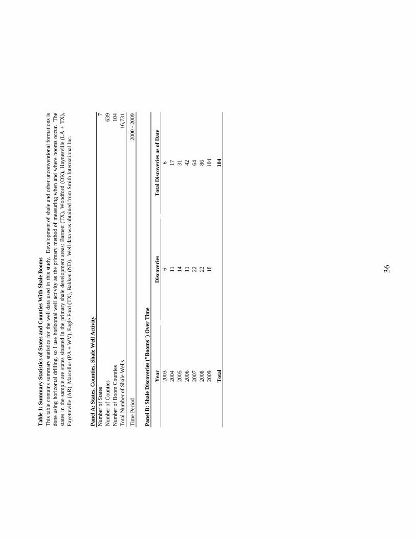
For my panel data set I include the seven states that have experienced shale booms from

2000 through 2009. These are Arkansas, Louisiana, North Dakota, Oklahoma, Pennsylvania,

Texas, and West Virginia. There are 639 counties in these states with at least one bank

branch over the sample period. Each of these states have counties that have experienced

shale booms, as well as counties which have not, and it is these non-boom county-years

which serve as the control group in empirical tests. The data is constructed on an annual

frequency and compiled from four di�erent sources:

• Well Data (From Smith International Inc.)

• Deposit and Bank Data (From FDIC Summary of Deposits Reports)

• County Level Economic Outcome Data by Industry (Census Bureau, Establishment

and Employment Data)

• External Finance Dependence Measures (From Compustat)

13

4.1 Well Data

Well data is used to calculate the Boomi,t variables in the regressions. The well data is ob-

tained from Smith International Inc. which provides detailed information on the time (year),

place (county), and type (horizontal or vertical) of well drilling activity. I use horizontal

wells as the key measure of shale development activity, as the majority of horizontal wells in

the U.S. drilled after 2002 target shale or other unconventional formations. In order to best

measure the in�uence of shale development activity I focus on two di�erent measures.

• Boomi,t = Dummyi,t : A dummy variable set to 1 if county i at time t is in the

top quartile of all county-years with shale well activity (total shale wells > 17) in the

panel dataset. Once the variable is set to 1, all subsequent years in the panel for the

county are set to 1. Based on this de�nition 88.1% of all shale wells are drilled in boom

county-years.

• Boomi,t = Log Total Shale Wellsi,t : The logarithm of the total number of shale wells

drilled in county i from 2003 to time t.

Regressions are based on the total shale wells drilled for the year leading up through March.

This corresponds to when the County Business Pattern Data are tabulated. Summary statis-

tics on sample states, counties, and well data are presented in Table 1. Figure 2 presents a

map of the intensity and location of shale development activity.

4.2 Deposit and Bank Data

Deposit and bank data are obtained from the Federal Deposit Insurance Corporation (FDIC)

Summary of Deposit data, which is reported on June 30 of each year and provides bank data

for all FDIC-insured institutions. I use the Summary of Deposit data as opposed to data

from the Reports of Condition and Income (Call Reports) because Summary of Deposit

14

data provides deposit data at the branch level, while Call Reports only provide data at the

bank level. Additionally, Summary of Deposit data provides detailed information on the

geographic location of each branch that a bank has, so I can directly observe the branches

in boom counties and the banks they belong to. To obtain county level deposit data I sum

deposits across all branches in a county. To calculate small bank market share in a county

I calculate the proportion of branches in a county which belong to small banks. I de�ne

small banks to be banks with assets below a threshold which could cause a bank to be

funding constrained. For the results in this paper I use $500 million (year 2003 dollars) as

the asset threshold for small banks.9 Prior literature (Black and Strahan (2002), Jayaratne

and Morgan (2000), Strahan and Weston (1998)), has suggested that banks with assets in

the $100 million to $500 million range may be funding constrained. In my empirical tests I

use two measures of small bank market share. Speci�cally, I use dummy variables set to 1

for the counties with the highest small bank branch market share (top quartile) in each year,

and 0 otherwise. Additionally, I also use the ratio of small bank branches to total branches

in a county. Summary data for bank and branch variables are provided in Table 2.

4.3 County Level Economic Outcome Data by Industry

Economic outcome variable data by industry was obtained from the County Business Pat-

terns survey, which is released annually by the Census Bureau. It is worth noting, that

the survey provides data only on establishments, not �rms, for example, a �rm may have

many establishments. The survey provides detailed data on establishments and employment

in each county, by North American Industry Classi�cation System (NAICS) code as of the

9 I document that the main results remain statistically signi�cant when using $200 million or $1 billion

in assets as the de�nition of a small bank. The results are also robust to basing this de�nition o� of bank

holding company assets.

15

week of March 12 every year. My main results are based on economic outcomes grouped

at the two digit NAICS code level, which I match with corresponding Compustat two digit

NAICS code external �nance dependence measures. More disaggregated NAICS codes (six

digit NAICS as opposed to two digit NAICS) provide fewer NAICS code matches to Com-

pustat, which I rely on for external �nance dependence measures. I exclude codes 21 (Oil

and Gas Extraction), 23 (Construction), 52 (Financials), 53 (Real Estate) because they may

be directly in�uenced by booms. I exclude 99 (Other) due to lack of comparability with

Compustat �rms. However, my results remain similar and statistically signi�cant when any

of these industries are included.10

After matching County Business Pattern data with Compustat external �nance depen-

dence measures, I aggregate all industry codes into two industry groups, one with above

median dependence on external �nance (high) and one with below median dependence on

external �nance (low). The two digit NAICS code from the County Business Patterns data is

used to obtain an external �nance dependence measure from Compustat, which is described

in more detail in the next subsection. The objective of the matching is to have the clean-

est sorting of NAICS codes into high external �nance dependence and low external �nance

dependence bins. Details on the industries in these bins are provided in Table 3.

While the County Business Patterns Survey provides detailed data on establishment

counts by industry, employment data may be suppressed, for privacy reasons, if there are

too few establishments in a particular industry. Employment data suppression is a particular

problem for counties with smaller populations, for this reason the number of observations in

employment regressions is reduced. Furthermore, this suppression of employment data makes

including employment in the regressions related to small bank market share problematic, as

62% of establishments in high small bank market share counties have employment reporting

suppressed.

10Using three digit NAICS code industries poses two problems 1) There are 71 industries as opposed to14, so there are far fewer comparable Compustat �rms for some industries 2) There was a change in industrycategorization that occurred in 2002-2003, which creates problems when constructing a pre-boom controlperiod for booms that occur in 2003 and 2004.

16

4.4 External Finance Dependence Measures

I use an external �nance dependence measure similar to the measure used by Rajan and

Zingales (1998). The main di�erence is that while they use this measure only for manufac-

turing �rms, I use it for all industry groups similar to Becker (2007). Speci�cally, over the

1999 to 2008 time period for each �rm in Compustat I sum the di�erence between capital

expenditures and operating cash �ow. I use the time period 1999 to 2008 because these

�scal years, which end in December for most public �rms, correspond most closely to March

of the following year (2000 to 2009), which is when the county business patterns survey is

conducted. By summing over several years the measure is less susceptible to being driven by

short term economic �uctuations. I then divide this sum by the sum of capital expenditures.

Speci�cally, for �rm n, the measure is calculated as:

ExtF inDependencen =

∑20081999(CapitalExpendituresn,t −OperatingCashF lown,t)∑2008

1999CapitalExpendituresn,t

I take the median of this measure to get an industry's external �nance dependence. The cal-

culation of this measure for each industry is displayed in Table 3. The underlying assumption

in the Rajan and Zingales (1998) measure is that some industries, for technological reasons,

have greater dependence on external �nancing than others. The measure is based on public

�rms in the United States which have among the best access to capital of any �rms in the

world, therefore the amount of capital used by these �rms is likely the best estimate that can

be obtained of an industry's true demand for external �nancing.

17

5 Results

5.1 E�ect of Shale Booms on Deposit Levels

Table 4 provides regression results of log deposits on di�erent shale boom variables. The

evidence suggests a causal relationship between shale booms and bank deposits, speci�cally,

that the individual mineral wealth generated by shale booms translates into more bank

deposits. In Panel A of Table 4 columns (1) and (2) provide results on di�erent measures

of the Boomi,t variable. In each case, the Boomi,t variable is found to have both economic

and statistical signi�cance. For example, the dummy variable measure of Boomi,t can be

interpreted as a boom increasing local deposits by 8.2%. To put this in context, the average

annual growth rate in deposits across all counties from 2000 to 2009 was 4.6%, so a boom

county would experience an additional increase of 8.2% (4.6% + 8.2% = 12.8% total increase),

or a total increase in deposits roughly triple its average annual increase.

Further tests will focus on comparisons between counties with high small bank market

share and low small bank market share. An assumption in this comparison is that both types

of counties experience similar deposit shocks. To directly test this assumption I estimate in-

teractions of county bank size characteristics interacted with the shale boom variables. Panel

B reports the results of this speci�cation. The key coe�cient of interest in assessing whether

counties experience di�erent shocks based on their banking structure is the coe�cient on the

interaction term (β4). This coe�cient is neither economically nor statistically signi�cant,

suggesting that counties with di�erent banking structure receive similar deposit shocks.

An additional concern may be that deposits could be rising in anticipation of a boom, or

that there could be some spurious correlation in a county during part of the boom period

which is causing the result in Table 4. To test the precise timing of the boom relative to

deposit growth I replace the boom dummy variable used in Table 4 with dummy variables

based on the position of an observation relative to a boom. So, for example, if a boom

occurs in 2006 in county i, then the observation in county i in 2003 would receive a t-3

18

boom dummy, county i observation in 2004 would receive the t-2 boom dummy and so on.

I include a set of dummies for each year relative to a boom from t-3 to t+3. Due to limited

observations beyond t+3, I group any observations after t+3 with the t+3 dummy (3+).

Figure 3 is a graph of the coe�cients from this regression, and provides visual evidence that

the deposit level does not change substantially until time 0, the �rst year of the boom. This

serves to alleviate concerns regarding whether deposits rise in anticipation of a boom, as well

as concerns about possible spurious correlations during part of the boom period.

5.2 E�ect of Credit Supply Shock on Economic Outcomes

Table 5 provides the results of the e�ect the shale boom on log establishments for all

industries industry types (high external �nance dependent and low external �nance depen-

dent). The economic interpretation of the results in column (1) is that the establishment

levels of all industries increases by 2.2% in a county when there is a boom. However, demand

for goods and services for all establishments may increase when there is a boom, so it is not

surprising to see the results in Table 5. In order to draw a more direct causal relationship

between the credit supply shock associated with a shale boom and economic outcomes, it is

necessary to look at the di�erence between outcomes for industries with a high dependence

on external �nance compared to those with low dependence on external �nance. In Table

6 I estimate the regression speci�cation in Table 5 on each industry group separately. The

larger magnitude of coe�cients in the regressions for industries more dependent on external

�nance (Ind = High) suggest that the industries in this industry group bene�t more from a

boom. Speci�cally, the coe�cients from (1) of Panel A in Table 6 can be interpreted as a

4.5% increase in high external �nance dependent establishments when a boom occurs relative

to no increase in low external �nance dependent establishments.11

There may be some concerns as to the timing of the boom and changes in local economic

11I document in Appendix A that for banks that have all branches in a single county, both deposits andCommercial & Industrial loans increase after a boom. Overall interest income and interest paid on depositsare unchanged after a boom. Lending driven purely by demand would be more likely to result in higherinterest rates and interest income.

19

outcomes. If establishment levels of low external �nance dependent industries and high

external �nance dependent industries trend di�erently prior to the boom, they may be poor

control/treatment groups. Additionally, if external �nance dependent establishments trend

higher well before the boom, it would suggest a problem with my empirical design, as the

deposit levels in Figure 3 do not increase until time 0. To directly assess the validity of these

concerns I construct a graph similar to Figure 3, but for establishments. Speci�cally, for each

of the industry groups I run the regressions in (1) and (2) of Table 6, but replace the Boomi,t

variable with a set of dummy variables based on the time period of an observation relative

to a boom for any given county i (similar to what is done in Figure 3). The coe�cients

from this regression are graphed for each industry group in Figure 4. As can be seen, from

time t-3 to t-1, each industry group tracks relatively closely, then at time 0, the �rst year

of a boom, there is a divergence in trends, which increases through t+3. This indicates

that when the boom occurs, establishments in high external �nance dependent industries

bene�t disproportionately more compared to low external �nance dependent industries. The

evidence presented in Figure 4 should serve to address concerns regarding the change in

establishment levels relative to the precise timing of a boom. The results outlined in Panel

A of Table 6 and Figure 4 can be formalized in a regression form of di�erences-in-di�erences.

Panel B of Table 6 provides a direct test of the evidence presented in Panel A of Table 6

and Figure 4 in a regression form of di�erences-in-di�erences. The coe�cient of interest for

assessing whether improved local credit supply plays a role in local economic outcomes is the

interaction term Boomi,t ∗ Highj. The sign and magnitude of this term indicates whether

one industry group bene�ts disproportionately when there is a boom. The coe�cient on the

interaction term is positive and statistically signi�cant in all speci�cations, suggesting that

local economic outcomes for industries more dependent on external �nance bene�t more than

outcomes for industries with low dependence on external �nance. The economic interpreta-

tion of the interaction coe�cient in (1) of Panel B of Table 6 is that, when there is a boom,

establishments in industries with high dependence on external �nance increase 4.6% relative

to establishments in industries with low dependence on external �nance. To put this number

in context, the average annual increase in high external �nance dependent establishments

20

from 2000 to 2009 is 0.9%.

5.3 E�ect of Bank Size and Credit Supply on Economic Outcomes

As previously discussed, local bank size composition could play a role in the importance

of improved local credit supply for economic outcomes. Speci�cally, counties dominated by

small banks may bene�t more from a credit supply shock. To test this in the di�erences-in-

di�erences framework, I subdivide counties into high small bank market share and low small

bank market share counties, based on whether a county is in the top quartile of small bank

market share in a given year. I estimate the speci�cation presented in Panel B of Table 6 for

each of these subgroups, and present the results in Table 7.

In every speci�cation the counties dominated by small banks have a higher coe�cient

for the interaction term Boomi,t ∗Highj. The magnitude of di�erences is often quite large,

with high small bank market share counties (Bank = High Small Bank Mkt Share) having

coe�cients more than �ve times the coe�cients of low small bank market share counties

(Bank = Low Small Bank Mkt Share), depending on the speci�cation. In order to address

concerns regarding anticipation and spurious correlations, I graph coe�cients as in Figure

4, but further subdivide high external �nance and low external �nance industries by bank

size characteristics to form four separate subgroups in Figure 5. As can be seen, all sub-

groups trend similarly until time 0, when the subgroup that comprises high external �nance

dependent industries in high small bank market share counties trends higher.

To formally test the results in Table 7 and Figure 5, I estimate a regression form of

di�erences-in-di�erences-in-di�erences, with the results shown in Table 8. This is done by

adding additional interactions with small bank market share variables. The coe�cient of

interest in these tests is the triple interaction term Boomi,t ∗Highj ∗ Small Banki,t. A posi-

tive coe�cient on the triple interaction term indicates that high external �nance dependent

industries bene�t more when there is a boom in an area with high small bank market share.

Speci�cally, the interpretation of (1) in Table 8 is that high external �nance dependent es-

tablishments increase by 10.9% relative to establishments in industries with low dependence

on external �nance in boom counties dominated by small banks relative to other boom coun-

21

ties. Across all speci�cations the coe�cient on Boomi,t ∗ Highj ∗ Small Banki,t is positive

and statistically signi�cant, providing formal evidence that higher small bank market share

counties were funding constrained prior to the boom. Speci�cally, if there were no frictions,

additional deposits from the boom should not disproportionately bene�t high external �nance

dependent industries in high small bank market share counties.

The results in Table 8 also address concerns regarding alternative explanations from

the prior di�erences-in-di�erences tests conducted. An important concern is whether high

external �nance dependent industries disproportionately bene�t from a boom for a reason

other than the credit supply component of a boom. For example, it could be the case that

high external �nance dependent industries bene�t more in general when there is an economic

boom (high asset beta). However, this explanation would not account for the di�erential

impact experienced in high small bank market share counties relative to low small bank

market share counties. An additional concern may be that there could be more demand for

goods and services for industries in the high external �nance dependence industry group.

However, in order for this explanation to be consistent with the results in Table 8, there

would also need to be a rationale for why this demand di�erential is relatively higher in

counties with high small bank market share. In summary, the results in Table 8 provide

added robustness for the initial di�erences-in-di�erences tests, while also documenting that

frictions are more problematic in counties dominated by small banks.

5.3.1 Alternative Measures of Economic Outcomes

The results presented in the main tests use logarithm of establishments as the primary eco-

nomic outcome measure. Table 9 reports the results of speci�cations that use the logarithm

of employment, establishments per capita, and logarithm of establishments per capita as eco-

nomic outcome measures. The results for these alternative measures are consistent with the

results reported in Table 6 and Table 8. One primary drawback of using employment data

as an economic outcome measure is that in many areas it is suppressed for privacy reasons.

22

5.4 Robustness

5.4.1 Sensitivity of Results to Industry Classi�cations

A potential concern with my empirical design is whether local economic outcomes for in-

dustries more dependent on external �nance improve relative to outcomes for industries less

dependent on external �nance for some reason other than improved local credit supply. The

di�erences-in-di�erences-in-di�erences tests help rule out several alternative explanations,

however, an additional test of this assumption is included in Table 10. Speci�cally, for each

industry group I calculate a measure of exposure to underlying economic �uctuations, asset

beta, using two di�erent asset beta methodologies.

βAsset1 =βEquity

1 + (1− Tax Rate) ∗ DebtEquity

βAsset2 =βEquity

1 + DebtEquity

The asset betas used are industry median asset betas. If it is the case that the asset betas for

each industry group are di�erent it could be cause for concern, as this would suggest that one

industry group would be more sensitive to overall �uctuations in an economy. The results

in Panel A of Table 10 provide evidence that the high external �nance dependent industry

group does have a higher asset beta. However, when the two highest asset beta industry

groups are dropped from the regressions causing both industry groups to have similar asset

betas, as in Panel B of Table 10, the interaction and triple interaction coe�cients from

the di�erences-in-di�erences regression and di�erences-in-di�erences-in-di�erences regression

are still positive and statistically signi�cant. This suggests that the di�erence in underlying

asset betas between the groups is not driving my main results. Additionally Table 10 provides

evidence that the regression results presented in Table 6 and Table 8 are not being driven by

any single industry group, and either its inclusion (Panel A (3) and (4)) or exclusion (Panel

C (3) and (4)) in the study.

23

5.4.2 Falsi�cation Tests

A potential concern in di�erences-in-di�erences tests is whether results are driven by pre-

existing trends or are otherwise anticipated. To directly test whether any of the local

economic outcome changes begin prior to a boom, I include dummy variables for the two

years prior to the �rst shale development. These enter the regressions in the form of the

False Boomi,t variable. As can be seen in the results in Table 11, neither the False Boomi,t

variable, nor any of the interaction variables are statistically signi�cant. This result provides

direct evidence that the changes in economic outcome variables documented in this paper do

not occur prior to the onset of shale development activity, and that there are no statistically

signi�cant pre-existing trends. Furthermore, because shale discoveries occur in di�erent years

in di�erent counties (not just a single event in all counties at the same time), alternative in-

terpretations of results would need to address changes in economic outcomes that happen to

coincide with boom events in di�erent locations at di�erent points in time.

I conduct a second falsi�cation test to assess whether growth shocks in general favor one

industry group over another. Speci�cally, in Table 12 I use data from the states immediately

adjacent to the seven shale states to test whether generic growth shocks or �booms� bene�t

one set of industries or counties dominated by small banks. False Boomi,t dummy variables

are inserted after high growth county-years so that the number of false boom county years

is approximately the same proportion of shale boom county years obtained in the main

sample (roughly 5% of all county-years). The key coe�cient of interest to test whether high

external �nance dependent industries always bene�t when there is growth in an area is on

the interaction term False Boomi,t ∗ Highj, this coe�cient is not statistically signi�cant.

Additionally, the triple interaction term False Boomi,t ∗ Highj ∗ Small Banki,t is neither

positive nor statistically signi�cant. These results suggest that the credit component of shale

booms make shale growth shocks unique from general localized growth shocks.

5.4.3 Bank Size, Bank Holding Companies, Post-Boom Banking Market Changes

The main results in this study categorize any bank with fewer than $500 million in

24

assets as a small bank. However, existing literature has sometimes used di�erent small

bank de�nitions. Additionally, banks that are part of larger bank holding companies may

have fewer funding constraints than banks that are not (Houston et al. (1997)). Table 13

reports regression results that use di�erent small bank asset thresholds: $200 million, $500

million, $1 billion (DeYoung et al. (2004)). Coe�cients on the key interaction term of interest

Boomi,t ∗Highj ∗ Small Banki,t are positive and statistically signi�cant, indicating that the

primary results reported in this paper are robust to alternate de�nitions of small bank.

Additionally, categorizing banks based o� of bank holding company assets does not alter the

main results.

There could be some concern that a county's bank size composition endogenously changes

after a shale discovery. To address this concern I estimate regressions that hold banking

market structure constant as of last year prior to a boom. These results are reported in

Table 14. The coe�cients on the triple interaction term are similar in magnitude to the main

speci�cations in Table 8 and remain statistically signi�cant. While bank structure could be

endogenous in a given year, it is unlikely that it is changed due to the anticipation of a boom.

Therefore local bank structure is not correlated with whether a county is treated (experiences

a boom) or not. Furthermore, the results from Table 14 indicate that if bank structure is

changing after a boom, it does not alter the main results signi�cantly.

6 Conclusions

The United States has one of the most developed banking systems in the world. Prior

research has demonstrated that deregulation, the adoption of lending technology and securiti-

zation, have led to improved economic outcomes. However, this paper provides new evidence

that, despite improvements, economically signi�cant frictions still remain in the U.S. banking

system. I use oil and gas shale discoveries to obtain exogenous variation in local credit supply

to document the economic magnitudes of these frictions. When there is a positive local credit

supply shock, economic outcomes for industries with more dependence on external �nance

25

improve relative to industries with less dependence on external �nance, suggesting that local

credit supply matters for economic outcomes.

The importance of local credit supply is linked to local bank size. Consistent with the

view that either small banks are funding constrained or are in areas with more �soft� informa-

tion borrowers, counties dominated by small banks experience a �vefold higher bene�t from

a local credit supply shock. These �ndings suggest that deregulation, increased use of lend-

ing technology and securitization have not fully alleviated economically important frictions,

particularly in areas dominated by small banks.

26

References

Ashcraft, A. B., 2005. Are banks really special? New evidence from the fdic-induced failure

of healthy banks. American Economic Review 95, 1712�1730.

Bassett, B., Brady, T., 2002. What drives the persistent competitiveness of small banks?

Finance and Economics Discussion Series working paper 2002-28 Board of Governors of

the Federal Reserve System.

Becker, B., 2007. Geographical segmentation of US capital markets. Journal of Financial

Economics 85, 151�178.

Berger, A. N., 2003. The economic e�ects of technological progress: Evidence from the

banking industry. Journal of Money, Credit and Banking 35, 141�176.

Berger, A. N., Miller, N., Petersen, M. A., Rajan, R. G., Stein, J. C., 2005. Does function

follow organizational form? Evidence from the lending practices of large and small banks.

Journal of Financial Economics 76, 237�269.

Berger, A. N., Rosen, R. J., Udell, G. F., 2007. Does market size structure a�ect competition?

The case of small business lending. Journal of Banking and Finance 31, 11�33.

Berger, A. N., Udell, G. F., 2006. A more complete conceptual framework for SME �nance.

Journal of Banking and Finance 30, 2945�2966.

Bertrand, M., Schoar, A., Thesmar, D., 2007. Banking deregulation and industry structure:

Evidence from the french banking reforms of 1985. Journal of Finance 62, 597�628.

Black, S. E., Strahan, P., 2002. Entrepreneurship and bank credit availability. Journal of

Finance 57, 2807�2833.

Butler, A. W., Cornaggia, J., 2011. Does access to external �nance improve productivity?

Evidence from a natural experiment. Journal of Financial Economics 99, 184�203.

27

Campello, M., 2002. Internal capital markets in �nancial conglomerates: Evidence from small

bank responses to monetary policy. Journal of Finance 57, 2773�2805.

Cetorelli, N., Strahan, P., 2006. Finance as a barrier to entry: Bank competition and industry

structure in local U.S. markets. Journal of Finance 61, 437�461.

Chava, S., Purnanandam, A., 2011. The e�ect of banking crisis on bank-dependent borrowers.

Journal of Financial Economics 99, 116�135.

Cornaggia, J., 2012. Does risk management matter? Evidence from the U.S. agriculture

industry. Journal of Financial Economics forthcoming.

DeYoung, R., Frame, W., D.Glennon, Nigro, P., 2011. The information revolution and small

business lending: The missing evidence. Journal of Financial Services Research 39, 19�33.

DeYoung, R., Hunter, W. C., Udell, G. F., 2004. The past, present, and probable future for

community banks. Journal of Financial Services Research 25, 85�133.

Guiso, L., Sapienza, P., Zingales, L., 2004. Does local �nancial development matter? Quar-

terly Journal of Economics 119, 929�969.

Houston, J., James, C., Marcus, D., 1997. Capital market frictions and the role of internal

capital markets in banking. Journal of Financial Economics 46, 135�164.

Iyer, R., Peydro, J., 2011. Interbank contagion at work: Evidence from a natural experiment.

Review of Financial Studies 24, 1337�1377.

Jayaratne, J., Morgan, D., 2000. Capital market frictions and deposit constraints at banks.

Journal of Money, Credit and Banking 32, 74�92.

Jayaratne, J., Strahan, P., 1996. The �nance-growth nexus: Evidence from bank branch

deregulation. Quarterly Journal of Economics 111, 639�670.

Kashyap, A., Stein, J. C., 2000. What do a million observations on banks say about the

transmission of monetary policy. American Economic Review 90, 407�428.

28

Kerr, W. R., Nanda, R., 2009. Democratizing entry: Banking deregulations, �nancing con-

straints and entrepreneurship. Journal of Financial Economics 94, 124�149.

Khwaja, A. I., Mian, A., 2008. Tracing the impact of bank liquidity shocks: Evidence from

an emerging market. American Economic Review 98, 1413�1442.

Loutskina, E., Strahan, P. E., 2009. Securitization and the declining impact of bank �nance

on loan supply: Evidence from mortgage originations. Journal of Finance 64, 861�889.

Paravisini, D., 2008. Local bank �nancial constraints and �rm access to external �nance.

Journal of Finance 63, 2161�2193.

Peek, J., Rosengren, E., 2000. Collateral damage: E�ects of the Japanese bank crisis on real

activity in the United States. American Economic Review 90, 30�45.

Petersen, M. A., Rajan, R. G., 2002. Does distance still matter? The information revolution

in small business lending. Journal of Finance 57, 2533�2570.

Plosser, M., 2011. Bank heterogeneity and capital allocation: Evidence from 'fracking' shocks.

Working Paper.

Rajan, R. G., Zingales, L., 1998. Financial dependence and growth. American Economic

Review 88, 559�586.

Schnabl, P., 2011. The international transmission of bank liquidity shocks: Evidence from an

emerging market. Journal of Finance forthcoming.

Stein, J. C., 2002. Information production and capital allocation: Decentralized versus hier-

archical �rms. Journal of Finance 57, 1891�1921.

Strahan, P. E., Weston, J. P., 1998. Small business lending and the changing structure of the

banking industry. Journal of Banking and Finance 22, 821�845.

Times-Picayune, 2008. `SWEET SPOT; A recent rush on natural gas drilling in northwest

louisiana is turning many landowners into instant millionaires, and stoking others' hopes

September 17.

29

Wall Street Journal, 2011. Oil without apologies April 15.

Yergin, D., 2011. The Quest: Energy, Security, and the Remaking of the Modern World. The

Penguin Press.

30

4) 6)

0%5%10%

15%

20%

25%

30%

35%

40%

0%10%

20%

30%

40%

50%

60%

70%

80%

2000 (0)

2001 (0)

2002 (0)

2003 (1)

2004

(18)

2005

(97)

2006

(361

)20

07(9

05)

2008

(164

4)20

09(2

336)

Establishment Percent Change vs. 2000 Level

Deposit Percent Change vs. 2000 Level

Year

(Num

ber

of S

hale

Wel

ls)

John

son

Cou

nty,

TX

Dep

osits

Low

Ext

erna

l Fin

ance

Dep

ende

nt In

dust

ries

Hig

h Ex

tern

al F

inan

ce D

epen

dent

Indu

strie

s

Pre-

Boo

mPo

st-B

oom

Figu

re1:

Boo

m C

ount

y, J

ohns

on C

ount

y, T

X: T

his f

igur

e pl

ots

the

rela

tive

chan

ge in

dep

osits

leve

ls a

nd e

stab

lishm

ent l

evel

s in

John

son

Cou

nty,

TX

. Es

tabl

ishm

ents

are

div

ided

into

two

indu

stry

gro

ups,

high

ext

erna

l fin

ance

dep

ende

nt in

dust

ries

and

low

ext

erna

l fin

ance

dep

ende

nt in

dust

ries.

The

num

bers

in p

aren

thes

is u

nder

the

year

s on

the

x-ax

is a

re th

e to

tal n

umbe

r of s

hale

w

ells

dril

led

in th

e co

unty

by

that

poi

nt in

tim

e.

31

Figu

re2:

Loc

atio

n an

d In

tens

ity o

f Sha

le A

ctiv

ityTh

e fig

ure

map

s the

cou

ntie

s of t

he 7

shal

e bo

om st

ates

incl

uded

in th

is st

udy:

OK

, TX

, LA

, WV

, PA

, ND

and

AR

. W

hite

cou

ntie

s are

cou

ntie

s with

no

shal

e de

velo

pmen

t act

ivity

. Th

e re

mai

ning

cou

ntie

s are

shad

ed b

ased

on

inte

nsity

of a

ctiv

ity re

late

d to

the

tota

l num

ber o

f sha

le w

ells

dril

led

thro

ugh

2009

.

TXLA

WV

PA

ND

AR

OK

Most A

ctive Quintile

LeastA

ctive Quintile

No Ac

tivity

32

Figu

re 3

: Dep

osit

Lev

els B

efor

e an

d A

fter

Sha

le B

oom

This

figur

epl

ots

the

regr

essi

onof

dum

my

varia

bles

base

don

the

year

rela

tive

toa

boom

.Th

efir

stye

arof

abo

omis

year

0,an

dth

ede

finiti

onof

boom

that

isus

edis

Boo

mD

umm

y(p

revi

ously

defin

ed).

For

exam

ple,

the

first

poin

tis

the

plot

ofa

dum

my

varia

ble

for

time

t-3re

lativ

eto

the

boom

.D

ueto

limite

dob

serv

atio

nsfo

rtim

esgr

eate

rth

ant+

3,al

lobs

erva

tions

afte

rtim

et+

3ar

egr

oupe

dw

ithth

et+

3du

mm

y(3

+).

The

depe

nden

tvar

iabl

eis

the

loga

rithm

ofto

tald

epos

itsin

the

coun

ty,

soth

eco

effic

ient

sca

nbe

inte

rpre

ted

asth

epe

rcen

tage

chan

gein

the

leve

lofd

epos

itsat

diff

eren

tpoi

ntsi

ntim

ere

lativ

eto

the

boom

. Th

e lo

garit

hm o

f pop

ulat

ion,

yea

r fix

ed e

ffec

ts, a

nd c

ount

y fix

ed e

ffec

ts w

ere

incl

uded

in th

e re

gres

sion

as w

ell.

0%2%4%6%8%10%

12%

14%

16%

18%

20%

-3-2

-10

12

3+

% Change in Deposit Level

Dep

osit

Lev

els B

efor

e an

d A

fter

Sha

le B

oom

Dep

osit

Coe

ffic

ient

Pre-

Boo

m

P

ost-B

oom

33

Figu

re 4

: E

stab

lishm

ent L

evel

s Bef

ore

and

Aft

er C

redi

t Sup

ply

Shoc

kTh

isfig

ure

plot

sse

para

tely

the

regr

essi

onco

effic

ient

sof

dum

my

varia

bles

ofth

eye

arre

lativ

eto

abo

omfo

rind

ustri

esw

ithhi

ghde

pend

ence

onex

tern

alfin

ance

and

low

depe

nden

ceon

exte

rnal

finan

ce.

The

first

year

ofa

boom

isye

ar0,

and

the

defin

ition

ofbo

omth

atis

used

isB

oom

Dum

my

(pre

viou

slyde

fined

).Fo

rex

ampl

e,th

efir

stpo

inti

sth

epl

otof

adu

mm

yva

riabl

efo

rtim

et-3

rela

tive

toth

ebo

om.

Due

tolim

ited

obse

rvat

ions

fort

imes

grea

tert

han

t+3,

allo

bser

vatio

nsaf

tert

ime

t+3

are

grou

ped

with

the

t+3

dum

my

(3+)

.Th

ede

pend

entv

aria

ble

islo

garit

hmof

esta

blis

hmen

tsin

anin

dust

ryin

aco

unty

,so

the

coef

ficie

ntsc

anbe

inte

rpre

ted

asth

epe

rcen

tage

chan

gein

esta

blish

men

tlev

els

atdi

ffer

entp

oint

sin

time

rela

tive

toth

ebo

om.

The

loga

rithm

of p

opul

atio

n, y

ear f

ixed

eff

ects

, and

cou

nty

fixed

eff

ects

wer

e in

clud

ed in

the

regr

essi

on a

s wel

l.

-2%0%2%4%6%8%10%

12%

14%

-3-2

-10

12

3+

% Change in Establishment Level

Eff

ect o

f Cre

dit S

uppl

y Sh

ock

on E

cono

mic

Out

com

es

Hig

h D

epen

denc

e on

Ext

erna

l Fin

ance

Low

Dep

ende

nce

on E

xter

nal F

inan

ce

Pre-

Boo

m

P

ost-B

oom

34

Figu

re 5

: Eff

ect o

f Cre

dit S

uppl

y Sh

ock

on C

ount

ies w

ith D

iffer

ent B

ank

Size

sTh

isfig

ure

plot

sse

para

tely

the

regr

essi

onco

effic

ient

sof

dum

my

varia

bles

ofth

eye

arre

lativ

eto

abo

omfo

rdi

ffer

ent

subg

roup

s.Sp

ecifi

cally

four

diff

eren

tgr

oup

desi

gnat

ions

are

used

base

don

whe

ther

anes

tabl

ishm

ent

has

high

orlo

wde

pend

ence

onex

tern

alfin

ance

and

whe

ther

itis

ina

coun

tyw

ithhi

ghor

low

smal

lban

km

arke

tsha

re.

The

first

year

ofa

boom

isye

ar0,

and

the

defin

ition

ofbo

omth

atis

used

isB

oom

Dum

my

(pre

viou

slyde

fined

).Fo

rexa

mpl

e,th

efir

stpo

inti

sth

epl

otof

adu

mm

yva

riabl

efo

rtim

et-3

rela

tive

toth

ebo

om.

Due

tolim

ited

obse

rvat

ions

for

times

grea

ter

than

t+3,

all

obse

rvat

ions

afte

rtim

et+

3ar

egr

oupe

dw

ithth

et+

3du

mm

y(3

+).

The

depe

nden

tvar

iabl

eis

loga

rithm

ofes

tabl

ishm

ents

inan

indu

stry

ina

coun

ty,s

oth

eco

effic

ient

sca

nbe

inte

rpre

ted

asth

epe

rcen

tage

chan

gein

esta

blis

hmen

tlev

els

atdi

ffer

ent

poin

tsin

time

rela

tive

toth

ebo

om.

The

loga

rithm

ofpo

pula

tion,

year

fixed

effe

cts,

and

coun

tyfix

edef

fect

swer

ein

clud

edin

the

regr

essi

on a

s wel

l.

-10%-5%0%5%10%

15%

20%

25%

30%

35%

-3-2

-10

12

3+

% Change in Establishment Level

Eff

ect o

f Cre

dit S

uppl

y Sh

ock

On

Diff

eren

t Sub

grou

ps

Hig

h Sm

all B

ank

+ H

igh

Ext F

in D

epLo

w S

mal

l Ban

k +

Hig

h Ex

t Fin

Dep

Hig

h Sm

all B

ank

+ Lo

w E

xt F

in D

epLo

w S

mal

l Ban

k +

Low

Ext

Fin

Dep

Pre-

Boo

m

P

ost-B

oom

35

Tab

le 1

: Sum

mar

y St

atis

tics o

f Sta

tes a

nd C

ount

ies W

ith S

hale

Boo

ms

Pane

l A: S

tate

s, C

ount

ies,

Shal

e W

ell A

ctiv

ityN

umbe

r of S

tate

s7

Num

ber o

f Cou

ntie

s63

9N

umbe

r of B

oom

Cou

ntie

s10

4To

tal N

umbe

r of S

hale

Wel

ls16

,731

Tim

e Pe

riod

2000

- 20

09

Pane

l B: S

hale

Dis

cove

ries

("B

oom

s") O

ver

Tim

e

Yea

rD

isco

veri

esT

otal

Dis

cove

ries

as o

f Dat

e20

036

620

0411

1720

0514

3120

0611

4220

0722

6420

0822

8620

0918

104

Tot

al10

4

This

tabl

eco

ntai

nssu

mm

ary

stat

istic

sfo

rth

ew

elld

ata

used

inth

isst

udy.

Dev

elop

men

tof

shal

ean

dot

heru

ncon

vent

iona

lfor

mat

ions

isdo

neus

ing

horiz

onta

ldril

ling,

soI

use

horiz

onta

lwel

lact

ivity

asth

epr

imar

ym

etho

dof

mea

surin

gw

hen

and

whe

rebo

oms

occu

r.Th

est

ates

inth

esa

mpl

ear

est

ates

situ

ated

inth

epr

imar

ysh

ale

deve

lopm

enta

reas

:Bar

nett

(TX

),W

oodf

ord

(OK

),H

ayne

svill

e(L

A+

TX),

Faye

ttevi

lle (A

R),

Mar

cellu

s (PA

+ W

V),

Eagl

e Fo

rd (T

X),

Bak

ken

(ND

). W

ell d

ata

was

obt

aine

d fr

om S

mith

Inte

rnat

iona

l Inc

.

36

Tab

le 2

: Pan

el R

egre

ssio

n Su

mm

ary

Stat

istic

s Obs

Mea

nSt

d D

ev

Dep

osits

Log

Dep

osits

6,38

212

.60

1.41

Dep

osits

($ in

thou

sand

s)6,

382

1,19

5,25

35,

228,

131

Eco

nom

ic O

utco

mes

Log

Esta

blis

hmen

ts12

,764

5.24

1.44

Esta

blis

hmen

ts12

,764

680

2,19

3

Con

trol

/Exp

lana

tory

Var

iabl

esLo

g To

tal S

hale

Wel

ls12

,764

0.45

1.07

Smal

l Ban

k B

ranc

h M

arke

t Sha

re12

,764

0.63

0.30

Log

Popu

latio

n12

,764

10.0

81.

40Po

pula

tion

12,7

6475

,938

229,

054

This

tabl

eco

ntai

nssu

mm

ary

stat

istic

sfo

rthe

data

used

inth

epa

nelr

egre

ssio

ns.

The

unit

ofob

serv

atio

nfo

rec

onom

icou

tcom

eva

riabl

esin

the

pane

lis

atth

eco

unty

-yea

r-in

dust

ry(e

xter

nal

finan

cein

dust

rygr

oup)

leve

l,w

hile

the

unit

ofob

serv

atio

nfo

rba

nkde

posi

tsis

atth

eco

unty

-yea

rle

vel.

Dat

aon

esta

blis

hmen

tsan

dem

ploy

men

tar

efr

omth

eC

ount

yB

usin

ess

Patte

rns

surv

ey.

Econ

omic

outc

ome

varia

bles

are

sum

med

acro

ssal

lind

ustri

esin

totw

ogr

oups

base

don

anin

dust

ry's

depe

nden

ceon

exte

rnal

finan

ce.

Hen

cefo

reac

hco

unty

-yea

rthe

rear

etw

oin

dust

rygr

oups

,one

with

high

depe

nden

ceon

exte

rnal

finan

cean

don

ew

ithlo

wde

pend

ence

onex

tern

alfin

ance

.D

ata

onan

nual

popu

latio

nle

vels

are

from

the

Cen

sus

Bur

eau.

Smal

lBan

ksar

eca

tego

rized

asba

nks

with

less

than

$500

mill

ion

inas

sets

,adj

uste

dfo

rin

flatio

n(y

ear2

003

dolla

rs).

Ban

kda

taw

asco

mpi

led

from

the

FDIC

Sum

mar

yof

Dep

osit

repo

rts.

Shal

ew

ell i

nfor

mat

ion

is b

ased

on

wel

l dat

a ob

tain

ed fr

om S

mith

Inte

rnat

iona

l Inc

.

37

Tab

le 3

: Ext

erna

l Fin

ance

Dep

ende

nce

of In

dust

ries

Tw

o D

igit

NA

ICS

Tw

o D

igit

NA

ICS

Nam

eE

xter

nal D

epen

denc

e M

easu

reE

xter

nal D

epen

denc

e Fl

ag

62H

ealth

Car

e an

d So

cial

Ass

ista

nce

-0.8

70

42W

hole

sale

Tra

de-0

.79

011

Agr

icul

ture

, For

estry

, Fis

hing

and

Hun

ting

-0.4

30

61Ed

ucat

iona

l Ser

vice

s-0

.43

081

Oth

er S

ervi

ces (

exce

pt P

ublic

Adm

inis

tratio

n)-0

.29

044

Ret

ail T

rade

-0.2

00

22U

tiliti

es-0

.14

056

Adm

inis

trativ

e an

d Su

ppor

t and

Was

te M

anag

emen

t and

Rem

edia

tion

Serv

ices

-0.0

11

48Tr

ansp

orta

tion

and

War

ehou

sing

-0.0

11

31M

anuf

actu

ring

0.16

172

Acc

omm

odat

ion

and

Food

Ser

vice

s0.

181

71A

rts, E

nter

tain

men

t, an

d R

ecre

atio

n0.

451

54Pr

ofes

sion

al, S

cien

tific

, and

Tec

hnic

al S

ervi

ces

0.81

151

Info

rmat

ion

0.95

1

This

tabl

ere

ports

the

indu

stry

grou

psus

edin

this

stud

y.Th

ein

dust

rygr

oups

are

base

don

the

two

digi

tN

orth

Am

eric

anIn

dust

ryC

lass

ifica

tion

Syst

emus

edin

the

repo

rting

ofth

eC

ount

yB

usin

ess

Patte

rns

surv

ey,w

hich

isre

porte

dan

nual

lyby

the

Cen

sus

Bur

eau.

Fore

ach

indu

stry

am

easu

reof

depe

nden

ceon

exte

rnal

finan

ceis

calc

ulat

ed,b

ased

onth

em

etho

dus

edby

Raj

anan

dZi

ngal

es(1

998)

.Th

eex

tern

alde

pend

ence

mea

sure

repo

rted

fore

ach

indu

stry

isth

ein

dust

rym

edia

nde

pend

ence

onex

tern

alfin

ance

.Th

eda

taus

edto

calc

ulat

eth

eex

tern

alfin

ance

depe

nden

cem

easu

reis

from

Com

pust

atfo

rthe

perio

dfr

om19

99to

2008

(the

fisca

lyea

rsth

atar

ecl

oses

tto

the

Mar

chda

taco

llect

ion

ofth

eC

ount

yB

usin

ess

Patte

rns

surv

eyfr

om20

00to

2009

).Th

eec

onom

icou

tcom

em

easu

resu

sed

are

aggr

egat

edin

totw

ose

para

tein

dust

rygr

oups

inea

chco

unty

,one

with

abov

em

edia

nde

pend

ence

onex

tern

alfin

ance

(Ext

erna

lDep

ende

nce

Flag

=1)

,and

one

with

belo

wm

edia

nde

pend

ence

onex

tern

alfin

ance

(Ext

erna

l Dep

ende

nce

Flag

= 0

).

38

Ta

ble

4: E

ffec

t of S

hale

Boo

ms o

n B

ank

Dep

osits

Pane

l A: E

ffec

t of S

hale

Boo

ms o

n B

ank

Dep

osits

Boo

m =

Dum

my

Boo

m =

Log

Tot

al S

hale

Wel

ls(1

)(2

)

Boo

mi,t

0.08

2***

0.02

2***

(4.0

9)(3

.80)

Log

Popu

latio

n i,t

0.56

2***

0.54

6***

(3.1

6)(3

.10)

Yea

r FE t

Yes

Yes

Cou

nty

FEi

Yes

Yes

R2

0.65

80.

659

N6,

382

6,38

2

Pane

l B: E

ffec

t of S

hale

Boo

m o

n B

ank

Dep

osits

: Cou

ntie

s With

Diff

eren

t Ban

k Si

zes

Boo

m =

Dum

my

Boo

m =

Log

Tot

al S

hale

Wel

ls(1

)(2

)

Boo

mi,t

0.09

2***

0.02

2***

(3.8

4)(3

.39)

Smal

l Ban

k i,t

-0.0

06-0

.008

(-0.

54)

(-0.

65)

Boo

mi,t

* S

mal

l Ban

k i,t

-0.0

38-0

.002

(-1.

04)

(-0.

21)

Log

Popu

latio

n i,t

0.55

9***

0.54

6***

(3.1

5)(3

.07)

Yea

r FE t

Yes

Yes

Cou

nty

FEi

Yes

Yes

R2

0.65

90.

659

N6,

382

6,38

2

This

tabl

ere

ports

the

resu

ltsof

regr

essi

ons

whi

chm

easu

reth

eef

fect

ofdi

ffer

entb

oom

varia

bles

onde

posi

ts.

The

depe

nden

tvar

iabl

ein

thes

ere

gres

sion

sis

the

log

ofto

tald

epos

itsin

coun

tyi

inye

art.

The

expl

anat

ory

varia

bles

are

diff

eren

tsha

lebo

omva

riabl

es,w

hich

have

prev

ious

lybe

ende

fined

.Lo

gof

coun

typo

pula

tion

isin

clud

edas

aco

ntro

l,as

are

coun

tyan

dye

arfix

edef

fect

s.Pa

nelA

docu

men

tsth

eef

fect

ofa

shal

ebo

omon

coun

tyba

nkde

posi

ts,

whi

lePa

nelB

test

sw

heth

erth

ere

isa

diff

eren

tiale

ffec

ton

bank

depo

sits

base

don

loca

lban

ksi

ze.

The

Smal

lBan

kD

umm

yva

riabl

eus

edin

Pane

lBis

equa

lto

1if

aco

unty

isin

the

top

quar

tile

ofsm

allb

ank

bran

chm

arke

tsha

rein

agi

ven

year

,and

0ot

herw

ise.

The

defin

ition

ofsm

allb

ank

inth

ese

regr

essi

ons

isan

yba

nkw

ithle

ssth

an$5

00m

illio

nin

asse

tsad

just

edfo

rinf

latio

n.St

anda

rder

rors

are

clus

tere

dby

coun

ty,w

itht-s

tatis

tics

repo

rted

inpa

rent

hese

s bel

ow c

oeff

icie

nt e

stim

ates

, whe

re *

indi

cate

s sig

nific

ance

at t

he 1

0% le

vel,

** a

t the

5%

leve

l, an

d **

* at

the

1% le

vel.

Smal

l Ban

k =

Dum

my

Log

Dep

osits

i,t =

α+ β 1

Log

Popu

latio

n i,t+ β 2

Boom

i,t+

Year

FE t

+ C

ount

y FE

i + ε

i,t

Log

Dep

osits

i,t =

α+ β 1

Log

Popu

latio

n i,t

+ β 2

Boom

i,t+ β 3

Smal

l Ban

k i,t

+ β 4

Boom

i,t *

Sm

all B

ank i,

t + Y

ear F

E t+

Cou

nty

FEi +

εi,t

39

Tab

le 5

: Eff

ect o

f Sha

le B

oom

on

Eco

nom

ic O

utco

mes

Boo

m =

Dum

my

Boo

m =

Log

Tot

al S

hale

Wel

ls(1

)(2

)

Boo

mi,t

0.02

2***

0.00

5**

(2.9

4)(2

.28)

Log

Popu

latio

n i,t

0.69

1***

0.68

9***

(16.

49)

(16.

31)

Indu

stry

Tren

ds F

E j,t

Yes

Yes

Cou

ntyI

ndus

try F

E i,j

Yes

Yes

R2

0.26

10.

260

N12

,764

12,7

64

This

tabl

ere

ports

the

resu

ltsof

regr

essi

ons

whi

chte

stth

ein

fluen

ceof

shal

ebo

oms

onec

onom

icou

tcom

es.

The

depe

nden

tvar

iabl

ein

thes

ere

gres

sion

sis

log

esta

blis

hmen

tsin

coun

tyi,

indu

stry

j,ye

art.

The

expl

anat

ory

varia

bles

are

diff

eren

tsha

lebo

omva

riabl

es,

whi

chha

vepr

evio

usly

been

defin

ed.

Log

ofco

unty

popu

latio

nis

also

incl

uded

asa

cont

rol,

asar

eco

unty

-indu

stry

and

indu

stry

-yea

r(in

dust

rytre

nds)

fixed

effe

cts.

Stan

dard

erro

rsar

ecl

uste

red

byco

unty

,w

itht-s

tatis

tics

repo

rted

inpa

rent

hese

sbe

low

coef

ficie

ntes

timat

es, w

here

* in

dica

tes s

igni

fican

ce a

t the

10%

leve

l, **

at t

he 5

% le

vel,

and

***

at th

e 1%

leve

l.

Log

Esta

blis

hmen

tsi,j

,t = α

+ β 1

Log

Popu

latio

n i,t

+ β 2

Boom

i,t+

Indu

stry

Tren

ds F

E j,t

+ C

ount

yInd

ustr

y FE

i,j +

εi,j

,t

40

Tab

le 6

: Eff

ect o

f Cre

dit S

uppl

y Sh

ock

on E

cono

mic

Out

com

es: D

iffer

ence

s-in

-Diff

eren

ces

(Boo

m v

s. N

on-B

oom

, Hig

h E

xt F

inan

ce D

epen

denc

e vs

. Low

Ext

Fin

ance

Dep

ende

nce)

Pane

l A

Ind

= H

igh

Ind

= Lo

wIn

d =

Hig

hIn

d =

Low

(1)

(2)

(3)

(4)

Boo

mi,t

0.04

5***

-0.0

020.

010*

**-0

.001

(3.2

6)(-

0.19

)(2

.90)

(-0.

55)

Log

Popu

latio

n i,t

0.68

8***

0.69

5***

0.68

2***

0.69

6***

(13.

14)

(17.

39)

(12.

97)

(17.

18)

Yea

r FE t

Yes

Yes

Yes

Yes

Cou

nty

FEi

Yes

Yes

Yes

Yes

R2

0.23

00.

328

0.22

90.

328

N6,

382

6,38

26,

382

6,38

2

Pane

l B

Boo

mi,t

Boo

mi,t

* H

igh j

Log

Popu

latio

n i,t

Indu

stry

Tren

ds F

E j,t

Cou

ntyI

ndus

try F

E i,j

R2

N

Boo

m =

Dum

my

Boo

m =

Log

Tot

al S

hale

Wel

ls

(-0.

52)

This

tabl

ere

ports

the

resu

ltsof

regr

essi

ons

mea

surin

gth

eef

fect

ofa

cred

itsu

pply

shoc

kon

diff

eren

tind

ustry

grou

ps,o

new

hich

has

high

depe

nden

ceon

exte

rnal

finan

ce(I

nd=

Hig

h)an

don

ew

hich

has

low

depe

nden

ceon

exte

rnal

finan

ce(I

nd=

Low

).Th

ede

pend

entv

aria

ble

inth

ese

regr

essi

ons

islo

ges

tabl

ishm

ents

.Pa

nelA

docu

men

tsth

edi

ffer

entia

leff

ecto

fth

ecr

edit

supp

lysh

ock

onin

dust

ries

with

high

depe

nden

ceon

exte

rnal

finan

cean

dth

ose

with

low

depe

nden

ceon

exte

rnal

finan

ce.

The

unit

ofob

serv

atio

nin

Pane

lA

islo

ges

tabl

ishm

ents

ofei

ther

Ind

=H

igh

orIn

d=

Low

inin

coun

tyi,

year

t.Pa

nelB

repr

esen

tsa

regr

essi

onfo

rmof

diff

eren

ces-

in-d

iffer

ence

san

dte

sts

whe

ther

the

cred

itsu

pply

shoc

kdi

ffer

entia

llyaf

fect

sin

dust

ries

with

high

exte

rnal

finan

cede

pend

ence

.Lo

gof

coun

typo

pula

tion

isal

soin

clud

edas

aco

ntro

l,as

are

coun

ty-in

dust

ryan

din

dust

ry-y

ear

(indu

stry

trend

s)fix

edef

fect

s.St

anda

rder

rors

are

clus

tere

dby

coun

ty,w

itht-s

tatis

tics

repo

rted

inpa

rent

hese

sbe

low

coef

ficie

ntes

timat

es,w

here

*in

dica

tes

sign

ifica

nce

atth

e10

%le

vel,

**at

the

5%le

vel,

and

***

at th

e 1%

leve

l. N

ote:

A c

oeff

icie

nt fo

r Hig

h j is

not

repo

rted

in P

anel

B, b

ecau

se it

is su

bsum

ed b

y C

ount

yInd

ustry

FE

i,j.

Boo

m =

Dum

my

Boo

m =

Log

Tot

al S

hale

Wel

ls

(1)

(2)

-0.0

01-0

.001

0.04

6***

(2.7

4)

(-0.

18)

0.26

312

,764

0.69

1***

0.01

2***

(2.6

8)

0.68

9***

(16.

31)

0.26

312

,764

Yes

Yes

Yes

(16.

48)

Yes

Log

Esta

blis

hmen

tsi,t

= α

+ β 1

Log

Popu

latio

n i,t

+ β 2

Boom

i,t+

Tim

e FE

t+

Cou

nty

FEi +

εi,t

Log

Esta

blis

hmen

tsi,j

,t = α

+ β 1

Log

Popu

latio

n i,t

+ β 2

Boom

i,t+ β 3

Hig

h j+ β 4

Boom

i,t *

Hig

h j+

Indu

stry

Tren

ds F

E j,t

+ C

ount

yInd

ustr

y FE

i,j +

εi,j

,t

41

Tab

le 7

: Eff

ect o

f Cre

dit S

uppl

y Sh

ock

on E

cono

mic

Out

com

es: S

ubdi

vide

d by

Sm

all B

ank

Mar

ket S

hare

(B

oom

vs.

Non

-Boo

m, H

igh

Ext

erna

l Fin

ance

Dep

ende

nce

vs. L

ow E

xter

nal F

inan

ce D

epen

denc

e)

Hig

h Sm

all B

ank

Mar

ket S

hare

Low

Sm

all B

ank

Mar

ket S

hare

Hig

h Sm

all B

ank

Mar

ket S

hare

Low

Sm

all B

ank

Mar

ket S

hare

(1)

(2)

(3)

(4)

Boo

mi,t

-0.0

160.

006

-0.0

070.

001

(-0.

70)

(0.9

1)(-

0.96

)(0

.54)

Boo

mi,t

* H

igh j

0.13

5***

0.02

5*0.

036*

*0.

007*

*(2

.60)

(1.9

3)(2

.33)

(2.1

2)

Log

Popu

latio

n i,t

0.41

2***

0.71

7***

0.40

5***

0.71

4***

(3.7

9)(1

3.47

)(3

.57)

(13.

38)

Indu

stry

Tren

ds F

E j,t

Yes

Yes

Yes

Yes

Cou

ntyI

ndus

try F

E i,j

Yes

Yes

Yes

Yes

R2

0.12

40.

398

0.12

00.

398

N3,

370

9,39

43,

370

9,39

4

Boo

m =

Dum

my

Boo

m =

Log

Tot

al H

oriz

onta

l Wel

ls

This

tabl

ere

ports

are

gres

sion

form

ofdi

ffer

ence

s-in

-diff

eren

ces

fort

wo

diff

eren

tcou

nty

grou

ps,o

neco

unty

grou

pw

hich

has

high

smal

lban

km

arke

tsha

re(B

ank

=H

igh

Smal

lBan

kM

ktSh

are)

,and

one

coun

tygr

oup

with

low

smal

lban

km

arke

tsha

re(B

ank

=Lo

wSm

allB

ank

Mkt

Shar

e).

The

defin

ition

ofsm

allb

ank

inth

ese

regr

essi

onsi

sany

bank

with

less

than

$500

mill

ion

inas

sets

adju

sted

fori

nfla

tion.

Fort

his

regr

essi

onhi

ghsm

allb

ank

mar

kets

hare

coun

tiesa

rede

fined

tobe

coun

ties

inth

eto

pqu

artil

eof

smal

lban

kbr

anch

mar

kets

hare

.Th

ede

pend

entv

aria

ble

inth

ese

regr

essi

ons

islo

gof

esta

blis

hmen

ts.

The

expl

anat

ory

varia

bles

are

diff

eren

tsh

ale

boom

varia

bles

,whi

chha

vepr

evio

usly

been

defin

ed.

Add

ition

ally

,an

inte

ract

ion

betw

een

boom

varia

bles

and

the

"Hig

h"ex

tern

alfin

ance

depe

nden

cedu

mm

yis

incl

uded

,thi

sis

the

diff

eren

ces-

in-d

iffer

ence

sco

effic

ient

ofin

tere

st(β

4).

Log

ofco

unty

popu

latio

nis

also

incl

uded

asa

cont

rol,

asar

eco

unty

-indu

stry

and

indu

stry

-ye

ar(in

dust

rytre

nds)

fixed

effe

cts.

Stan

dard

erro

rsar

ecl

uste

red

byco

unty

,with

t-sta

tistic

sre

porte

din

pare

nthe

ses

belo

wco

effic

ient

estim

ates

,whe

re*

indi

cate

ssi

gnifi

canc

eat

the

10%

leve

l,**

atth

e5%

leve

l,an

d**

*at

the

1%le

vel.

Not

e:A

coef

ficie

ntfo

rH

igh j

isno

tin

clud

edse

para

tely

,bec

ause

itis

subs

umed

byC

ount

yInd

ustry

FE i

,j .

Log

Esta

blis

hmen

tsi,j

,t = α

+ β 1

Log

Popu

latio

n i,t

+ β 2

Boom

i,t+ β 3

Hig

h j+ β 4

Boom

i,t *

Hig

h j+

Indu

stry

Tren

ds F

E j,t

+ C

ount

yInd

ustr

y FE

i,j +

εi,j

,t

42

Tab

le 8

: Eff

ect o

f Ban

k Si

ze a

nd C

redi

t Sup

ply

on O

utco

mes

: Diff

eren

ces-

in-D

iffer

ence

s-in

-Diff

eren

ces R

egre

ssio

n (B

oom

vs.

Non

-Boo

m, H

igh

Ext

Fin

ance

Dep

ende

nce

vs. L

ow E

xt F

inan

ce D

epen

denc

e, H

igh

Smal

l Ban

k M

arke

t Sha

re v

s. L

ow S

mal

l Ban

k M

arke

t Sha

re)

Smal

l Ban

k =

Dum

my

Smal

l Ban

k =

Rat

ioSm

all B

ank

= D

umm

ySm

all B

ank

= R

atio

(1)

(2)

(3)

(4)

Boo

mi,t

0.01

00.

034*

*0.

002

0.01

2***

(1.4

4)(2

.15)

(1.0

5)(3

.01)

Smal

l Ban

k i,t

-0.0

02-0

.016

0.00

3-0

.008

(-0.

27)

(-1.

07)

(0.4

4)(-

0.51

)

Boo

mi,t

* H

igh j

0.01

6-0

.065

*0.

005

-0.0

15*

(1.2

2)(-

1.82

)(1

.64)

(-1.

85)

Boo

mi,t

* S

mal

l Ban

k i,t

-0.0

42**

-0.0

55*

-0.0

15**

*-0

.021

***

(-2.

02)

(-1.

94)

(-2.

71)

(-3.

04)

Smal

l Ban

k i,t *

Hig

h j0.

003

0.02

3-0

.005

0.01

1(0

.25)

(0.9

4)(-

0.41

)(0

.45)

Boo

mi,t

* S

mal

l Ban

k i,t *

Hig

h j0.

109*

*0.

172*

**0.

027*

*0.

043*

**(2

.30)

(2.6

0)(2

.27)

(2.7

3)

Log

Popu

latio

n i,t

0.69

2***

0.69

4***

0.68

8***

0.68

9***

(16.

45)

(16.

39)

(16.

28)

(16.

22)

Indu

stry

Tren

ds F

E j,t

Yes

Yes

Yes

Yes

Cou

ntyI

ndus

try F

E i,j

Yes

Yes

Yes

Yes

R2

0.26

70.

268

0.26

70.

267

N12

,764

12,7

6412

,764

12,7

64

Boo

m =

Dum

my

Boo

m =

Log

Sha

le W

ells

This

tabl

ere

ports

resu

ltsfo

ra

regr

essi

onfo

rmof

diff

eren

ces-

in-d

iffer

ence

s-in

-diff

eren

ces,

whe

reth

eco

effic

ient

ofin

tere

stis

the

tripl

ein

tera

ctio

nte

rm.T

hede

pend

entv

aria

ble

inth

ese

regr

essi

ons

islo

ges

tabl

ishm

ents

inco

unty

i,ye

art,

indu

stry

grou

pj.

The

expl

anat

ory

varia

bles

are

diff

eren

tbo

omva

riabl

es,w

hich

have

prev

ious

lybe

ende

fined

.Th

ede

finiti

onof

smal

lban

kin

thes

ere

gres

sion

sis

any

bank

with

less

than

$500

mill

ion

inas

sets

adju

sted

fori

nfla

tion.

Thes

esp

ecifi

catio

nspr

ovid

ere

sults

fort

wo

diff

eren

tmea

sure

sof

Smal

lBan

k i,t.

One

mea

sure

isa

dum

my

varia

ble,

sett

o1

ifa

coun

tyis

inth

ehi

ghes

tqua

rtile

ofsm

allb

ank

bran

chm

arke

tsha

rein

any

give

nye

aran

d0

othe

rwis

e(S

mal

lBan

k=

Dum

my)

,whi

leth

eot

herm

easu

reis

the

ratio

ofbr

anch

esw

hich

belo

ngto

smal

lban

ksre

lativ

eto

the

tota

lnum

bero

fban

kbr

anch

esin

aco

unty

(Sm

allB

ank

=R

atio

).A

dditi

onal

ly,a

seto

fful

lysa

tura

ted

inte

ract

ions

betw

een

Boo

mva

riabl

es,S

mal

lBan

kva

riabl

es,a

ndth

eH

igh

exte

rnal

finan

cede

pend

ence

dum

my

are

incl

uded

.Th

eke

yco

effic

ient

ofin

tere

stfo

rth

edi

ffer

ence

s-in

-diff

eren

ces-

in-d

iffer

ence

sreg

ress

ion

isth

etri

ple

inte

ract

ion

term

β 8.

Log

ofco

unty

popu

latio

nis

also

incl

uded

asa

cont

rol,

asar

eco

unty

-indu

stry

and

indu

stry

-yea

r(in

dust

rytre

nds)

fixed

effe

cts.

Stan

dard

erro

rsar

ecl

uste

red

byco

unty

,with

t-sta

tistic

sre

porte

din

pare

nthe

ses

belo

wco

effic

ient

estim

ates

,whe

re*

indi

cate

ssi

gnifi

canc

eat

the

10%

leve

l, **

at t

he 5

% le

vel,

and

***

at th

e 1%

leve

l. N

ote:

A c

oeff

icie

nt fo

r Hig

h j is

not

repo

rted,

bec

ause

it is

subs

umed

by

Cou

ntyI

ndus

try F

E i,j .

Log

Esta

blis

hmen

tsi,j

,t = α

+ β 1

Log

Popu

latio

n i,t

+ β 2

Boom

i,t +

β3H

igh j

+ β 4

Smal

l Ban

k i,t +

β5B

oom

i,t *

Hig

h j +

β6B

oom

i,t *

Smal

l Ban

k i,t

+ β 7

Hig

h j *

Smal

l Ban

k i,t +

β8B

oom

i,t *

Smal

l Ban

k i,t *

Hig

h j +

Indu

stry

Tren

ds F

E j,t

+ C

ount

yInd

ustr

y FE i

,j + ε i,

j,t

43

Tab

le 9

: Alte

rnat

ive

Eco

nom

ic O

utco

me

Mea

sure

s

Out

com

e =

Log

Empl

oym

ent

(1)

(2)

(3)

(4)

(5)

Boo

mi,t

0.00

4-0

.402

*-0

.259

-0.0

04*

-0.0

01(0

.32)

(-1.

73)

(-1.

14)

(-1.

68)

(-0.

57)

Smal

l Ban

k i,t

-0.9

68-0

.001

(-1.

09)

(-0.

14)

Boo

mi,t

* H

igh j

0.03

5*0.

974*

**0.

575*

0.01

2***

0.00

5(1

.65)

(2.8

5)(1

.87)

(2.6

0)(1

.59)

Boo

mi,t

* S

mal

l Ban

k i,t

-0.6

43-0

.011

*(-

1.13

)(-

1.94

)

Smal

l Ban

k i,t *

Hig

h j0.

836

-0.0

06(0

.79)

(-0.

44)

Boo

mi,t

* S

mal

l Ban

k i,t *

Hig

h j1.

778*

*0.

030*

*(2

.16)

(2.2

2)

Log

Popu

latio

n i,t

0.79

7***

(17.

96)

Indu

stry

Tren

ds F

E j,t

Yes

Yes

Yes

Yes

Yes

Cou

ntyI

ndus

try F

E i,j

Yes

Yes

Yes

Yes

Yes

R2

0.14

20.

113

0.11

70.

096

0.10

2N

10,1

1212

,764

12,7

6412

,764

12,7

64

Out

com

e =

Esta

blis

hmen

ts P

er C

apita

Out

com

e =

Log

Esta

blis

hmen

ts P

er C

apita

This

tabl

ere

ports

resu

ltsfo

rth

ere

gres

sion

ses

timat

edin

Tabl

e6

(Diff

eren

ces-

in-D

iffer

ence

s)an

dTa

ble

8(D

iffer

ence

s-in

-Diff

eren

ces-

in-D

iffer

ence

s)w

ithdi

ffer

ent

econ

omic

outc

ome

mea

sure

s.Sp

ecifi

catio

n(1

)use

sLo

gEm

ploy

men

tas

anec

onom

icou

tcom

eva

riabl

e,w

hile

(2)a

nd(3

)use

esta

blis

hmen

tspe

rcap

ita(p

er10

,000

peop

le),

and

(4)a

nd(5

)use

log

esta

blis

hmen

tspe

rcap

ita.

Not

e,a

diff

eren

ces-

in-d

iffer

ence

s-in

-diff

eren

cess

peci

ficat

ion

isno

trep

orte

dfo

rLog

Empl

oym

entb

ecau

se62

%of

empl

oym

entd

ata

issu

ppre

ssed

coun

ties

with

high

smal

lban

km

arke

tsha

re.

Stan

dard

erro

rsar

ecl

uste

red

byco

unty

,with

t-sta

tistic

sre

porte

din

pare

nthe

ses

belo

wco

effic

ient

estim

ates

,whe

re*

indi

cate

ssi

gnifi

canc

eat

the

10%

leve

l,**

atth

e5%

leve

l,an

d**

*at

the

1%le

vel.

Not

e:A

coef

ficie

nt fo

r Hig

h j is

not

repo

rted,

bec

ause

it is

subs

umed

by

Cou

ntyI

ndus

try F

E i,j.

Boo

m =

Log

Sha

le W

ells

Smal

l Ban

k =

Dum

my

44

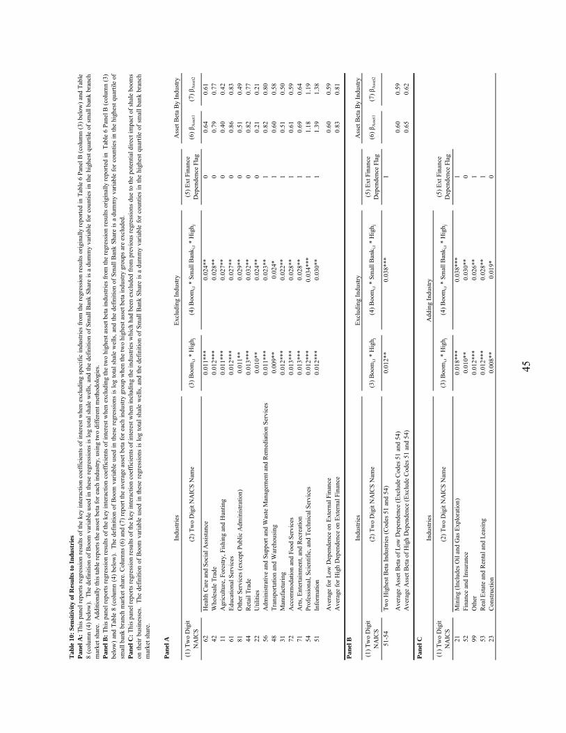
Tab

le 1

0: S

ensi

tivity

of R

esul

ts to

Indu

stri

es

Pane

l A

(1) T

wo

Dig

it N

AIC

S(2

) Tw

o D

igit

NA

ICS

Nam

e(3

) Boo

mi,t

* H

igh j

(4) B

oom

i,t *

Sm

all B

ank i

,t * H

igh j

(5) E

xt F

inan

ce

Dep

ende

nce

Flag

(6) β

Ass

et1

(7) β

Ass

et2

62H

ealth

Car

e an

d So

cial

Ass

ista

nce

0.01

1***

0.02

4**

00.

640.

6142

Who

lesa

le T

rade

0.01

2***

0.02

8**

00.

790.

7711

Agr

icul

ture

, For

estry

, Fis

hing

and

Hun

ting

0.01

1***

0.02

7**

00.

400.

4261

Educ

atio

nal S

ervi

ces

0.01

2***

0.02

7**

00.

860.

8381

Oth

er S

ervi

ces (

exce

pt P

ublic

Adm

inis

tratio

n)0.

011*

*0.

029*

*0

0.51

0.49

44R

etai

l Tra

de0.

013*

**0.

032*

*0

0.82

0.77

22U

tiliti

es0.

010*

*0.

024*

*0

0.21

0.21

56A

dmin

istra

tive

and

Supp

ort a

nd W

aste

Man

agem

ent a

nd R

emed

iatio

n Se

rvic

es0.

011*

**0.

023*

*1

0.82

0.80

48Tr

ansp

orta

tion

and

War

ehou

sing

0.00

9**

0.02

4*1

0.60

0.58

31M

anuf

actu

ring

0.01

2***

0.02

2**

10.

510.

5072

Acc

omm

odat

ion

and

Food

Ser

vice

s0.

013*

**0.

028*

*1

0.61

0.59

71A

rts, E

nter

tain

men

t, an

d R

ecre

atio

n0.

013*

**0.

028*

*1

0.69

0.64

54Pr

ofes

sion

al, S

cien

tific

, and

Tec

hnic

al S

ervi

ces

0.01

2***

0.03

4***

11.

181.

1951

Info

rmat

ion

0.01

2***

0.03

0**

11.

391.

38

Ave

rage

for L

ow D

epen

denc

e on

Ext

erna

l Fin

ance

0.60

0.59

Ave

rage

for H

igh

Dep

ende

nce

on E

xter

nal F

inan

ce0.

830.

81

Pane

l B

(1) T

wo

Dig

it N

AIC

S(2

) Tw

o D

igit

NA

ICS

Nam

e(3

) Boo

mi,t

* H

igh j

(4) B

oom

i,t *

Sm

all B

ank i

,t * H

igh j

(5) E

xt F

inan

ce

Dep

ende

nce

Flag

(6) β

Ass

et1

(7) β

Ass

et2

51-5

4Tw

o H

ighe

st B

eta

Indu

strie

s (C

odes

51

and

54)

0.01

2**

0.03

8***

1

Ave

rage

Ass

et B

eta

of L

ow D

epen

denc

e (E

xclu

de C

odes

51

and

54)

0.60

0.59

Ave

rage

Ass

et B

eta

of H

igh

Dep

ende

nce

(Exc

lude

Cod

es 5

1 an

d 54

)0.

650.

62

Pane

l C

(1) T

wo

Dig

it N

AIC

S(2

) Tw

o D

igit

NA

ICS

Nam

e(3

) Boo

mi,t

* H

igh j

(4) B

oom

i,t *

Sm

all B

ank i

,t * H

igh j

(5) E

xt F

inan

ce

Dep

ende

nce

Flag

21M

inin

g (I

nclu

des O

il an

d G

as E

xplo

ratio

n)0.

018*

**0.

038*

**1

52Fi

nanc

e an

d In

sura

nce

0.01

0**

0.03

0**

099

Oth

er0.

012*

**0.

026*

*1

53R

eal E

stat

e an

d R

enta

l and

Lea

sing

0.01

2***

0.02

8**

123

Con

stru

ctio

n0.

008*

*0.

019*

0

Indu

strie

sA

ddin

g In

dust

ry

Pane

lA:T

his

pane

lrep

orts

regr

essi

onre

sults

ofth

eke

yin

tera

ctio

nco

effic

ient

sof

inte

rest

whe

nex

clud

ing

spec

ific

indu

strie

sfr

omth

ere

gres

sion

resu

ltsor

igin

ally

repo

rted

inTa

ble

6Pa

nelB

(col

umn

(3)b

elow

)and

Tabl

e8

(col

umn

(4)b

elow

).Th

ede

finiti

onof

Boo

mva

riabl

eus

edin

thes

ere

gres

sions

islo

gto

tals

hale

wel

ls,an

dth

ede

finiti

onof

Smal

lBan

kSh

are

isa

dum

my

varia

ble

forc

ount

ies

inth

ehi

ghes

tqua

rtile

ofsm

allb

ank

bran

chm

arke

t sha

re.

Add

ition

ally

this

tabl

e re

ports

the

asse

t bet

a fo

r eac

h in

dust

ry, u

sing

two

diffe

rent

met

hodo

logi

es.

Pane

lB:T

his

pane

lrep

orts

regr

essi

onre

sults

ofth

eke

yin

tera

ctio

nco

effic

ient

sofi

nter

estw

hen

excl

udin

gth

etw

ohi

ghes

tass

etbe

tain

dust

riesf

rom

the

regr

essi

onre

sults

orig

inal

lyre

porte

din

Tabl

e6

Pane

lB(c

olum

n(3

)be

low

)and

Tabl

e8

(col

umn

(4)b

elow

).Th

ede

finiti

onof

Boo

mva

riabl

eus

edin

thes

ere

gres

sion

sis

log

tota

lsha

lew

ells,

and

the

defin

ition

ofSm

allB

ank

Shar

eis

adu

mm

yva

riabl

efo

rcou

ntie

sin

the

high

estq

uarti

leof

smal

l ban

k br

anch

mar

ket s

hare

. Col

umns

(6) a

nd (7

) rep

ort t

he a

vera

ge a

sset

bet

a fo

r eac

h in

dust

ry g

roup

whe

n th

e tw

o hi

ghes

t ass

et b

eta

indu

stry

gro

ups a

re e

xclu

ded.

Pane

lC:T

hisp

anel

repo

rtsre

gres

sion

resu

ltsof

the

key

inte

ract

ion

coef

ficie

ntso

fint

eres

twhe

nin

clud

ing

the

indu

strie

swhi

chha

dbe

enex

clud

edfr

ompr

evio

usre

gres

sion

sdue

toth

epo

tent

iald

irect

impa

ctof

shal

ebo

oms

onth

eirb

usin

esse

s.Th

ede

finiti

onof

Boo

mva

riabl

eus

edin

thes

ere

gres

sion

sis

log

tota

lsha

lew

ells,

and

the

defin

ition

ofSm

allB

ank

Shar

eis

adu

mm

yva

riabl

efo

rcou

ntie

sin

the

high

estq

uarti

leof

smal

lban

kbr

anch

mar

ket s

hare

.

Indu

strie

sEx

clud

ing

Indu

stry

Ass

et B

eta

By

Indu

stry

Indu

strie

sEx

clud

ing

Indu

stry

Ass

et B

eta

By

Indu

stry

45

Tab

le 1

1: F

alsi

ficat

ion

Tes

t of P

re-B

oom

Tre

nds

(1)

(2)

Boo

mi,t

-0.0

010.

002

(-0.5

5)(0

.86)

Fals

e B

oom

i,t-0

.001

-0.0

00(-0

.30)

(-0.0

8)

Smal

l Ban

k i,t

0.00

5(0

.58)

Boo

mi,t

* H

igh j

0.01

3***

0.00

6*(2

.81)

(1.7

8)

Fals

e B

oom

i,t *

Hig

h j0.

007

0.00

4(1

.37)

(0.7

4)

Boo

mi,t

* S

mal

l Ban

k i,t

-0.0

15**

*(-2

.76)

Fals

e B

oom

i,t *

Sm

all B

ank i

,t-0

.006

(-0.7

7)

Smal

l Ban

k Sh

are i,

t * H

igh j

-0.0

09(-0

.76)

Boo

mi,t

* S

mal

l Ban

k i,t *

Hig

h j0.

030*

*(2

.43)

Fals

e B

oom

i,t *

Sm

all B

ank i

,t * H

igh j

0.02

1(1

.25)

Log

Popu

latio

n i,t

0.68

9***

0.68

8***

(16.

28)

(16.

25)

Indu

stry

Tren

ds F

E j,t

Yes

Yes

Cou

ntyI

ndus

try F

E i,j

Yes

Yes

R2

0.26

30.

267

N12

,764

12,7

64

This

tabl

ere

ports

resu

ltsof

fals

ifica

tion

test

sfo

rthe

regr

essi

ons

inTa

bles

6an

d8.

Spec

ifica

lly,d

umm

yva

riabl

esar

ein

serte

dfo

rthe

two

year

spr

iort

oth

ebe

ginn

ing

ofsh

ale

wel

lac

tivity

.Th

ede

pend

entv

aria

ble

inth

ese

regr

essi

ons

islo

ges

tabl

ishm

ents

inco

unty

i,ye

art,

indu

stry

grou

pj.

Stan

dard

erro

rsar

ecl

uste

red

byco

unty

,with

t-sta

tistic

sre

porte

din

pare

nthe

ses

belo

wco

effic

ient

estim

ates

,whe

re*

indi

cate

ssi

gnifi

canc

eat

the

10%

leve

l,**

atth

e5%

leve

l,an

d**

*at

the

1%le

vel.

Not

e:A

coef

ficie

ntfo

rHig

h jis

noti

nclu

ded

sepa

rate

ly, b

ecau

se it

is su

bsum

ed b

y C

ount

yInd

ustry

FE i

,j .

Fals

e B

oom

= D

umm

y, B

oom

= L

og T

otal

Sha

le W

ells

Smal

l Ban

k =

Dum

my

(1) L

og E

stab

lishm

ents

i,j,t = α

+ β 1

Log

Popu

latio

n i,t

+ β 2

Boom

i,t +

β2F

Fals

e Bo

omi,t

+ β

3Hig

h j +

β4B

oom

i,t *

Hig

h j +

β4F

Fals

e Bo

omi,t

* H

igh j

+ In

dust

ryTr

ends

FE j

,t+

Cou

ntyI

ndus

try F

E i,j

+ ε i,

j,t

(2) L

og E

stab

lishm

ents

i,j,t = α

+ β 1

Log

Popu

latio

n i,t

+ β 2

Boom

i,t +

β2F

Fals

e Bo

omi,t

+ β

3Hig

h j+ β 4

Smal

l Ban

k i,t +

β5B

oom

i,t *

Hig

h j +

β5F

Fals

e Bo

omi,t

* H

igh j

+

β 6Bo

omi,t

* Sm

all B

ank i,

t + β

6FFa

lse

Boom

i,t *

Smal

l Ban

k i,t

+ β 7

Hig

h j *

Smal

l Ban

k i,t+

β8B

oom

i,t *

Smal

l Ban

k i,t *

Hig

h j

+ β 8

FFal

se B

oom

i,t *

Smal

l Ban

k i,t *

Hig

h j +

Indu

stry

Tren

ds F

E j,t

+ C

ount

yInd

ustr

y FE i

,j + ε i,

j,t

46

Tab

le 1

2: F

alsi

ficat

ion

Tes

t Usi

ng N

on-S

hale

Gro

wth

Sho

cks

(1)

(2)

Fals

e B

oom

i,t0.

152*

**0.

155*

**(1

0.52

)(9

.26)

Smal

l Ban

k i,t

0.00

5(0

.96)

Fals

e B

oom

i,t *

Hig

h j0.

002

0.01

1(0

.07)

(0.5

3)

Fals

e B

oom

i,t *

Sm

all B

ank i,

t-0

.008

(-0.

36)

Smal

l Ban

k i,t *

Hig

h j-0

.002

(-0.

26)

Fals

e B

oom

i,t *

Sm

all B

ank i,

t * H

igh j

-0.0

27(-

0.85

)

Log

Popu

latio

n i,t

0.69

2***

0.81

8***

(16.

45)

(26.

86)

Indu

stry

Tren

ds F

E j,t

Yes

Yes

Cou

ntyI

ndus

try F

E i,j

Yes

Yes

R2

0.30

70.

308

N22

,932

22,9

32

This

tabl

ere

ports

resu

ltsof

fals

ifica

tion

test

sfor

the

regr

essi

onsi

nTa

bles

6an

d8

usin

gno

n-sh

ale

grow

thbo

omsi

nst

ates

adja

cent

toth

ese

ven

shal

esta

tesi

nth

isst

udy.

Spec

ifica

lly,

dum

my

"Fal

seB

oom

"va

riabl

esar

ein

serte

daf

ter

high

grow

thco

unty

-yea

rssu

chth

atth

enu

mbe

rof

Fals

eB

oom

coun

tyye

ars

isap

prox

imat

ely

the

sam

epr

opor

tion

ofSh

ale

Boo

mco

unty

year

sob

tain

edin

the

mai

nsa

mpl

e(r

ough

ly5%

ofal

lco

unty

-yea

rs).

The

obje

ctiv

eof

this

spec

ifica

tion

isto

test

whe

ther

gene

ralg

row

thsh

ocks

diff

eren

tially

affe

cta

parti

cula

rin

dust

rygr

oup.

The

depe

nden

tvar

iabl

ein

thes

ere

gres

sion

sis

log

esta

blis

hmen

tsin

coun

tyi,

year

t,in

dust

rygr

oup

j.St

anda

rder

rors

are

clus

tere

dby

coun

ty,w

itht-

stat

istic

srep

orte

din

pare

nthe

sesb

elow

coef

ficie

ntes

timat

es,w

here

*in

dica

tess

igni

fican

ceat

the

10%

leve

l,**

atth

e5%

leve

l,an

d**

*at

the

1%le

vel.

Not

e:A

coef

ficie

ntfo

rHig

h j

is n

ot in

clud

ed se

para

tely

, bec

ause

it is

subs

umed

by

Cou

ntyI

ndus

try F

E i,j.

Fals

e B

oom

= D

umm

ySm

all B

ank

Shar

e =

Dum

my

47

Tab

le 1

3: A

ltern

ativ

e T

hres

hold

s for

Sm

all B

ank

Size

(Boo

m v

s. N

on-B

oom

, Hig

h E

xt F

inan

ce D

epen

denc

e vs

. Low

Ext

Fin

ance

Dep

ende

nce,

Hig

h Sm

all B

ank

Mar

ket S

hare

vs.

Low

Sm

all B

ank

Mar

ket S

hare

)

Smal

l Ban

k =

$500

M D

umm

yH

oldi

ng C

ompa

ny =

Yes

Hol

ding

Com

pany

= N

oH

oldi

ng C

ompa

ny =

Yes

Hol

ding

Com

pany

= N

oH

oldi

ng C

ompa

ny =

Yes

(1)

(2)

(3)

(4)

(5)

Boo

mi,t

0.00

20.

001

0.00

10.

002

0.00

2(1

.13)

(0.5

8)(0

.48)

(1.0

5)(1

.13)

Smal

l Ban

k i,t

0.00

30.

001

-0.0

010.

003

0.00

3(0

.43)

(0.1

9)(-

0.11

)(0

.44)

(0.4

3)

Boo

mi,t

* H

igh j

0.00

40.

007*

0.00

7*0.

005

0.00

4(1

.34)

(1.9

2)(1

.95)

(1.6

4)(1

.34)

Boo

mi,t

* S

mal

l Ban

k i,t

-0.0

16**

*-0

.009

**-0

.009

**-0

.015

***

-0.0

16**

*(-

2.98

)(-

2.25

)(-

1.98

)(-

2.71

)(-

2.98

)

Smal

l Ban

k i,t *

Hig

h j-0

.009

-0.0

03-0

.017

-0.0

05-0

.009

(-0.

78)

(-0.

22)

(-1.

44)

(-0.

41)

(-0.

78)

Boo

mi,t

* S

mal

l Ban

k i,t *

Hig

h j0.

032*

**0.

018*

*0.

019*

*0.

027*

*0.

032*

**(2

.76)

(2.0

9)(1

.98)

(2.2

7)(2

.76)

Log

Popu

latio

n i,t

0.68

9***

0.68

9***

0.68

9***

0.68

8***

0.68

9***

(16.

28)

(16.

30)

(16.

29)

(16.

28)

(16.

28)

Indu

stry

Tren

ds F

E j,t

Yes

Yes

Yes

Yes

Yes

Cou

ntyI

ndus

try F

E i,j

Yes

Yes

Yes

Yes

Yes

R2

0.26

80.

265

0.26

50.

267

0.26

8N

12,7

6412

,764

12,7

6412

,764

12,7

64

This

tabl

ere

ports

resu

ltsfo

rare

gres

sion

form

ofdi

ffer

ence

s-in

-diff

eren

ces-

in-d

iffer

ence

s,w

here

the

coef

ficie

ntof

inte

rest

isth

etri

ple

inte

ract

ion

term

.The

depe

nden

tvar

iabl

ein

thes

ere

gres

sion

sisl

oges

tabl

ishm

ents

inco

unty

i,ye

art,

indu

stry

grou

pj.

This

tabl

ere

ports

spec

ifica

tions

usin

gdi

ffer

ents

mal

lban

kde

finiti

ons.

The

regr

essi

ons

inth

ista

ble

repo

rtre

sults

fors

mal

lban

kcu

toff

sat

$200

mill

ion,

$500

mill

ion,

and

$1bi

llion

inas

sets

adju

sted

for

infla

tion.

Add

ition

ally

,the

spec

ifica

tions

repo

rtre

sults

for

asse

tsm

easu

red

both

atth

eba

nkle

vela

ndat

the

bank

hold

ing

com

pany

leve

l.Sm

allB

ank i

,tis

adu

mm

yva

riabl

e,se

tto

1if

aco

unty

isin

the

high

estq

uarti

leof

smal

lban

kbr

anch

mar

kets

hare

inan

ygi

ven

year

and

0ot

herw

ise

(Sm

allB

ank

=D

umm

y).

Ase

toff

ully

satu

rate

din

tera

ctio

nsbe

twee

nB

oom

varia

bles

,Sm

all

Ban

kva

riabl

es,

and

the

Hig

hex

tern

alfin

ance

depe

nden

cedu

mm

yar

ein

clud

ed.

The

key

coef

ficie

ntof

inte

rest

for

the

diff

eren

ces-

in-d

iffer

ence

s-in

-di

ffer

ence

sreg

ress

ion

isth

etri

ple

inte

ract

ion

term

β 8.

Log

ofco

unty

popu

latio

nis

also

incl

uded

asa

cont

rol,

asar

eco

unty

-indu

stry

and

indu

stry

-yea

r(in

dust

rytre

nds)

fixed

effe

cts.

Stan

dard

erro

rsar

ecl

uste

red

byco

unty

,with

t-sta

tistic

sre

porte

din

pare

nthe

ses

belo

wco

effic

ient

estim

ates

,whe

re*

indi

cate

ssi

gnifi

canc

eat

the

10%

leve

l,**

atth

e5%

leve

l,an

d**

*at

the

1%le

vel.

Not

e:A

coef

ficie

ntfo

r Hig

h j is

not

repo

rted,

bec

ause

it is

subs

umed

by

Cou

ntyI

ndus

try F

E i,j .

Smal

l Ban

k =

$20

0M D

umm

ySm

all B

ank

= $

1B D

umm

yB

oom

= L

og S

hale

Wel

ls

Log

Esta

blis

hmen

tsi,j

,t = α

+ β 1

Log

Popu

latio

n i,t

+ β 2

Boom

i,t +

β3H

igh j

+ β 4

Smal

l Ban

k i,t +

β5B

oom

i,t *

Hig

h j +

β6B

oom

i,t *

Smal

l Ban

k i,t

+ β 7

Hig

h j *

Smal

l Ban

k i,t +

β8B

oom

i,t *

Smal

l Ban

k i,t *

Hig

h j +

Indu

stry

Tren

ds F

E j,t

+ C

ount

yInd

ustr

y FE i

,j + ε i,

j,t

48

Tab

le 1

4: P

re-B

oom

Ban

king

Str

uctu

re R

obus

tnes

s

Smal

l Ban

k =

Dum

my

Smal

l Ban

k =

Rat

ioSm

all B

ank

= D

umm

ySm

all B

ank

= R

atio

(1)

(2)

(3)

(4)

Boo

mi,t

0.00

60.

041*

*0.

001

0.01

2***

(1.0

5)(2

.34)

(0.5

4)(2

.79)

Smal

l Ban

k i,t

0.00

9-0

.002

0.01

20.

003

(0.9

8)(-

0.15

)(1

.25)

(0.1

8)

Boo

mi,t

* H

igh j

0.02

0-0

.085

**0.

006*

-0.0

19**

(1.4

9)(-

2.42

)(1

.94)

(-2.

25)

Boo

mi,t

* S

mal

l Ban

k i,t

-0.0

25-0

.059

**-0

.008

-0.0

20**

*(-

1.23

)(-

1.98

)(-

1.55

)(-

2.64

)

Smal

l Ban

k i,t *

Hig

h j-0

.003

0.02

1-0

.009

0.01

0(-

0.21

)(0

.82)

(-0.

59)

(0.3

8)

Boo

mi,t

* S

mal

l Ban

k i,t *

Hig

h j0.

082*

0.18

2***

0.01

9*0.

045*

**(1

.91)

(2.9

2)(1

.70)

(2.8

1)

Log

Popu

latio

n i,t

0.69

2***

0.69

4***

0.68

9***

0.69

1***

(16.

47)

(16.

31)

(16.

25)

(16.

11)

Indu

stry

Tren

ds F

E j,t

Yes

Yes

Yes

Yes

Cou

ntyI

ndus

try F

E i,j

Yes

Yes

Yes

Yes

R2

0.26

60.

267

0.26

50.

267

N12

,764

12,7

6412

,764

12,7

64

This

tabl

ere

ports

resu

ltsfo

rare

gres

sion

form

ofdi

ffer

ence

s-in

-diff

eren

ces-

in-d

iffer

ence

s,w

here

the

coef

ficie

ntof

inte

rest

isth

etri

ple

inte

ract

ion

term

.Thi

sre

gres

sion

issi

mila

rto

the

regr

essi

onre

sults

repo

rted

inTa

ble

8,ho

wev

er,t

heba

nksi

zest

ruct

ure

ofa

coun

tyis

kept

the

sam

eas

the

year

prio

rto

expe

rienc

ing

abo

om.

The

depe

nden

tvar

iabl

ein

thes

ere

gres

sion

sis

log

esta

blis

hmen

tsin

coun

tyi,

year

t,in

dust

rygr

oup

j.Th

ese

spec

ifica

tions

prov

ide

resu

ltsfo

rtw

odi

ffer

entm

easu

res

ofSm

allB

ank i

,t.O

nem

easu

reis

adu

mm

yva

riabl

e,se

tto

1if

aco

unty

isin

the

high

estq

uarti

leof

smal

lban

kbr

anch

mar

kets

hare

inan

ygi

ven

year

and

0ot

herw

ise

(Sm

allB

ank

=D

umm

y),w

hile

the

othe

rmea

sure

isth

era

tioof

bran

ches

whi

chbe

long

tosm

allb

anks

rela

tive

toth

eto

taln

umbe

rofb

ank

bran

ches

ina

coun

ty(S

mal

lBan

k=

Rat

io).

Add

ition

ally

,ase

toff

ully

satu

rate

din

tera

ctio

nsbe

twee

nB

oom

varia

bles

,Sm

allB

ank

varia

bles

,and

the

Hig

hex

tern

alfin

ance

depe

nden

cedu

mm

yar

ein

clud

ed.

The

key

coef

ficie

ntof

inte

rest

fort

hedi

ffer

ence

s-in

-diff

eren

ces-

in-d

iffer

ence

sre

gres

sion

isth

etri

ple

inte

ract

ion

term

β 8.

Log

ofco

unty

popu

latio

nis

also

incl

uded

asa

cont

rol,

asar

eco

unty

-indu

stry

and

indu

stry

-yea

r(in

dust

rytre

nds)

fixed

effe

cts.

Stan

dard

erro

rsar

ecl

uste

red

byco

unty

,with

t-sta

tistic

sre

porte

din

pare

nthe

ses

belo

wco

effic

ient

estim

ates

,whe

re*

indi

cate

ssi

gnifi

canc

eat

the

10%

leve

l,**

atth

e5%

leve

l,an

d**

*at

the

1% le

vel.

Not

e: A

coe

ffic

ient

for H

igh j

is n

ot re

porte

d, b

ecau

se it

is su

bsum

ed b

y C

ount

yInd

ustry

FE i

,j.

Boo

m =

Dum

my

Boo

m =

Log

Sha

le W

ells

Log

Esta

blis

hmen

tsi,j

,t = α

+ β 1

Log

Popu

latio

n i,t

+ β 2

Boom

i,t +

β3H

igh j

+ β 4

Smal

l Ban

k i,t +

β5B

oom

i,t *

Hig

h j +

β6B

oom

i,t *

Smal

l Ban

k i,t

+ β 7

Hig

h j *

Smal

l Ban

k i,t +

β8B

oom

i,t *

Smal

l Ban

k i,t *

Hig

h j +

Indu

stry

Tren

ds F

E j,t

+ C

ount

yInd

ustr

y FE i

,j + ε i,

j,t

49

App

endi

x A

: Ban

k R

egre

ssio

ns fo

r B

anks

with

All

Bra

nche

s in

One

Cou

nty

Pane

l A

Out

com

e =

Log

Dep

osits

Out

com

e =

Log

C&

I Loa

nsO

utco

me

= In

tere

st R

ate

Out

com

e =

Dep

osit

In

tere

st R

ate

(1)

(2)

(3)

(4)

Boo

mi,t

0.09

19**

*0.

1007

**0.

0004

0.00

04(4

.11)

(2.3

2)(0

.13)

(1.0

9)

Log

Popu

latio

n i,t

0.24

65**

*0.

3920

***

-0.0

020

0.00

15**

*(4

.94)

(4.7

3)(-

0.94

)(2

.92)

Yea

r FE t

Yes

Yes

Yes

Yes

Ban

k FE

jY

esY

esY

esY

es

R2

0.39

90.

118

0.39

90.

872

N8,

176

8,17

68,

176

8,17

6

Pane

l B

Out

com

e =

Log

Dep

osits

Out

com

e =

Log

C&

I Loa

nsO

utco

me

= In

tere

st R

ate

Out

com

e =

Dep

osit

In

tere

st R

ate

(1)

(2)

(3)

(4)

Boo

mi,t

0.02

65**

*0.

0297

**-0

.000

70.

0000

(4.2

2)(2

.55)

(-0.

86)

(0.2

9)

Log

Popu

latio

n i,t

0.24

57**

*0.

3911

***

-0.0

020

0.00

15**

*(5

.08)

(4.7

1)(-

0.89

)(2

.92)

Yea

r FE t

Yes

Yes

Yes

Yes

Ban

k FE

jY

esY

esY

esY

es

R2

0.40

10.

119

0.39

90.

872

N8,

176

8,17

68,

176

8,17

6

This

tabl

ere

ports

the

resu

ltsof

regr

essi

onsw

hich

estim

ate

the

effe

ctof

diff

eren

tsha

lebo

omva

riabl

eson

bank

outc

omes

forb

anks

that

have

allo

fthe

irbr

anch

esin

asi

ngle

coun

ty.

The

unit

ofob

serv

atio

nin

this

pane

lis

coun

tyi,

bank

j,ye

art.

Dat

aon

bank

sw

asco

mpi

led

from

Cal

lRep

orts

and

Sum

mar

yof

Dep

osit

repo

rts.

Aba

nkis

inth

esa

mpl

eif

allo

fits

bran

ches

are

ina

sing

leco

unty

ingi

ven

year

,tre

atm

entb

anks

are

thos

eba

nks

whi

char

ein

shal

ebo

omco

unty

-yea

rs,w

hile

cont

rolb

anks

are

sing

leco

unty

bank

sin

non-

shal

ebo

omco

unty

-yea

rs.C

&Il

oans

are

the

tota

lam

ount

ofco

mm

erci

alan

din

dust

riall

oans

aba

nkre

ports

onits

Cal

lRep

ort.

Inte

rest

inco

me

isth

eto

tali

nter

esti

ncom

ea

bank

gene

rate

sin

aye

ar,d

ivid

edby

itsav

erag

eto

tall

oans

.D

epos

itIn

tere

stR

ate

isth

ein

tere

stpa

idon

alld

epos

itsdi

vide

dby

the

aver

age

amou

ntof

depo

sits

aba

nkha

sin

agi

ven

year

.B

oth

inte

rest

rate

and

depo

siti

nter

estr

ate

varia

bles

wer

ew

inso

rized

at1%

and

99%

.Lo

gof

coun

typo

pula

tion

isin

clud

edas

aco

ntro

l,as

are

year

fixed

effe

ctsa

ndba

nkfix

edef

fect

s.St

anda

rder

rors

are

clus

tere

dby

bank

,with

t-sta

tistic

sre

porte

din

pare

nthe

sesb

elow

coef

ficie

ntes

timat

es,w

here

*in

dica

tes

sign

ifica

nce

atth

e10

%le

vel,

**at

the

5%le

vel,

and

***

atth

e1%

leve

l.

Boo

m =

Dum

my

Boo

m =

Log

Tot

al S

hale

Wel

ls

Bank

Out

com

e i,j,t

= α

+ β 1

Log

Popu

latio

n i,t

+ β 2

Boom

i,t +

Yea

r FE t

+ Ba

nk F

E j+ ε i,

j,t

50

A

ppen

dix

B: D

iffer

ence

s-in

-Diff

eren

ces-

in-D

iffer

ence

s Reg

ress

ion,

Tab

le 8

Fix

ed E

ffec

t Rob

ustn

ess

(1)

(2)

(3)

(4)

(5)

(6)

Boo

mi,t

-0.0

00-0

.008

***

0.00

50.

002

(-0.

09)

(-3.

80)

(1.4

2)(1

.05)

Smal

l Ban

k Sh

are i,

t0.

064*

**0.

008

0.06

2***

0.00

3(5

.04)

(0.9

9)(4

.94)

(0.4

4)

Boo

mi,t

* H

igh j

0.01

0*0.

025*

**0.

000

0.00

50.

010*

0.00

0(1

.89)

(8.2

3)(0

.05)

(1.6

4)(1

.89)

(0.0

5)

Boo

mi,t

* S

mal

l Ban

k Sh

are i,

t-0

.023

***

-0.0

16**

*-0

.022

***

-0.0

15**

*(-

2.87

)(-

3.00

)(-

2.76

)(-

2.71

)

Smal

l Ban

k Sh

are i,

t * H

igh j

-0.1

26**

*-0

.015

-0.1

23**

*-0

.005

-0.1

26**

*-0

.123

***

(-5.

81)

(-1.

13)

(-5.

68)

(-0.

41)

(-5.

81)

(-5.

68)

Boo

mi,t

* S

mal

l Ban

k Sh

are i,

t * H

igh j

0.04

4***

0.03

1***

0.04

2***

0.02

7**

0.04

4***

0.04

2***

(2.9

7)(2

.63)

(2.8

1)(2

.27)

(2.9

7)(2

.81)

Log

Popu

latio

n i,t

0.68

8***

0.68

8***

0.68

8***

0.68

8***

(16.

29)

(16.

29)

(16.

28)

(16.

28)

Yea

r FE t

Yes

Yes

No

No

No

No

Indu

stry

Tren

ds F

E j,t

No

No

Yes

Yes

No

Yes

Cou

nty

FEi

Yes

No

Yes

No

No

No

Cou

ntyI

ndus

try F

E i,j

No

Yes

No

Yes

No

No

Cou

ntyY

ear F

E i,t

No

No

No

No

Yes

Yes

R2

0.79

40.

227

0.79

70.

267

0.81

70.

82N

12,7

6412

,764

12,7

6412

,764

12,7

6412

,764

Econ

omic

Out

com

e =

Log

Esta

blis

hmen

tsB

oom

= L

og T

otal

Sha

le W

ells

Smal

l Ban

k =

Dum

my

This

tabl

eco

ntai

nsth

esa

me

regr

essi

onsp

ecifi

catio

nas

Tabl

e8,

exce

ptfo

rthe

type

sof

fixed

effe

cts

used

.Th

ista

ble

prov

ides

resu

ltsfo

rvar

ious

com

bina

tions

ofIn

dust

ryTr

ends

FEj,t

, Yea

r FE t

, Cou

ntyI

ndus

try F

E i,j,

Cou

nty

FEi,

Cou

ntyY

ear F

E i,t.

51