1

Does Water Management Improve Corporate Value?∗

Valentin Jouvenot University of Geneva

Geneva Finance Research Institute

May 25, 2019

Preliminary and Incomplete. Please do not circulate.

Abstract

I examine whether water supply frictions affect corporate valuation and performance

using the occurrence of droughts as a source of exogenous variation. I present causal

evidence that investors value good water management because it allows firms to offset

the negative impact of droughts on operating expenses. Overall, the evidence supports

the hypothesis that good water management provides a competitive advantage for firms.

JEL classification : G32, L60, L25, Q54, Q25, Q56

Keywords: water management; firm performance; corporate value; climate change; sustainability

2

Water management plays an increasing role for investors.1 Yet, there remains

limited quantitative evidence of the economic benefits of water management at the

corporate level in developed countries. In particular, investors may wonder why firms

would invest in water management in the United States—a country with ample water

resources. In this paper, I examine whether and how water management increases firm

value. I provide causal evidence that investors value water management because it allows

firms to mitigate the damages of unexpected droughts.

Examining the potential effect of water management on firm valuations is

challenging for a least two reasons. First, it is unclear how to measure and define

corporate water management. Second, the relationship between water management and

firm value is endogenous. Although a change in water management may cause a change

in firm value, the opposite may also be true. Firms with high values, for example, may

invest more in water management than firms with low values.

To address the first challenge, I measure water management using readily

available firm-level measures from Morgan Stanley Capital International (MSCI). MSCI

water management scores capture the quality of a firm’s water management based on

qualitative and quantitative criteria such as the volume of recycled water, the number

of alternative water sources or whether water governance is part of the executive strategy

of a firm. To solve the identification challenge, I exploit geographic heat variations in

the form of drought surprises. Drought surprises, that is, the extent to which drought

intensities exceed the long-term average drought intensity in a given year are measured

1 Anecdotal evidence suggests that investors value water. For instance, in 2011 Norges Bank Investment Management, Norway’s Sovereign Wealth Fund managing about $950bn of assets, reiterated concerns over water scarcity (Norges, 2011). In 2014, Bloomberg and the Natural Capital declaration launched the water Risk Valuation Tools to help financial managers to assess how equity values could be exposed to risks from water stress. One year later, The Natural Capital Finance Alliance, RMS and GIZ supported by nine financial institutions representing more than US$10 trillion launched the Drought Stress Test. In 2015, Ceres, an environmental NGO, in collaboration with 40 institutional investors launched the Investor Water Hub to integrate water considerations into the investment decision process. In parallel, an increasing number of initiatives aimed at supporting investors and corporates to achieve water disclosure have been launched: see for instance, the Global Reporting Initiative, the Global Water Tool, or the Business Water Footprint. Lambooy (2011) or Sarni (2012) provide a complete review See also examples of proxy voting guidelines that reference water at https://engagements.ceres.org.

3

using variations in the Palmer Drought Severity Index (PDSI). The idea is that within

state variations in the drought index are exogenous and thus likely to create water supply

frictions.

Average values of good and bad water management firms when their headquarters are impacted by drought surprises. Firm value is measured by Tobin’s q. Shaded areas indicate 95% confidence interval. I calculate estimates using two-sided t-tests.

Figure 1 motivates my analysis. The figure plots the average values of firms with

good and bad water management when their headquarters are impacted by drought

surprises. I define good and bad water management firms relative to the sample median

MSCI water management score in a given year: while good firms correspond to firms

with above median MSCI scores, bad firms correspond to firms with below median MSCI

scores. The x-axis depicts the magnitude of a drought surprise. Negative drought surprise

values, on the left of the figure, correspond to unexpected wet weather; positive drought

surprise values, on the right of the figure, indicate unexpected droughts. A Drought

surprise equals to zero, in the middle, corresponds to the full distribution of weather.

The figure shows that during unexpected wet weather the values of good and bad firms

are virtually equivalent. In contrast, during unexpected droughts, the average value of

good firms increases significantly in comparison to the average value of bad firms. The

-4 -3 -2 -1 0 1 2 3 4

1.5

2

2.5

3

3.5

Good WM

Bad WM

DroughtWet Drought surprise

Fir

mvalu

e(Tobin

’sq)

Figure 1

31

4

effect is large: during the occurrence of drought surprises larger than or equal to three,

the average difference between the values of good and bad firms is around 0.72.

A natural concern is that such a sizable difference may be explained by other firm

characteristics than water management. For instance, large firms with high profitability

may afford the cost of good water management. Water-intensive industries or firms

headquartered in states with low water supplies may also have better water management

relative to low water-intensive industries or firms headquartered in states with frequent

precipitations.

To control for such different firm characteristics and isolate the causal effect of water

management on firm value, I exploit the occurrence of each drought surprises intensity

as a quasi-natural experiment. I use a difference-in-differences approach, comparing the

change in firm value between good and bad firms around the time of these drought

surprises. Controlling for a large number of state, industry and firm characteristics, I

find that the difference between the values of good and bad firms exhibit a similar

empirical pattern than in Figure 1; but the economic magnitude of this difference is

lower. For instance, during drought surprises with intensities larger than or equal to

three, the difference between the average values of good and bad firms is 14.14% relative

to the average Tobin’s q.

I then examine whether such a large difference in values during unexpected droughts

is driven by bad or good firms. To do so, I compare the values of good and bad firms

impacted by drought surprises to the value of a control group including firms that are

not impacted by drought surprises. I find that during extreme unexpected droughts, the

increase in value for good firms is of similar magnitude than the decrease in value for

bad firms. These similar magnitudes suggest that investors penalize bad firms as much

as they reward good water management.

Next, I ask why investors value water management. If investors see water management

as a positive predictor of future firm performance during unexpected droughts, we should

5

be able to identify such outperformance. I find evidence that the empirical pattern

observed for firm value in Figure 1 is explained by operating expenses. During extreme

unexpected droughts, the operating expenses of good firms decrease in comparison to the

operating expenses of bad firms. Such lower operating expenses support the view that

good water management allows firms to offset the negative impact of droughts on

operating performance. During the occurrence of drought surprises with intensities equal

or larger to three, for example, the average difference between the operating expenses of

good and bad firms is 6.47% relative to the average operating expenses.

Although operating expenses are significantly lower during drought conditions for

good firms relative to bad firms, they are also larger during wet conditions. Comparing

water management costs and benefits across the full distribution of drought surprises

provide evidence that good water management is an optimal investment: the costs due

to water management during wet weather exactly balance the water management

benefits of avoided damages during unexpected droughts. Thus, the results indicate that

investors value good water management because it reflects an effective adaptation to

unexpected droughts. By contrast, investors penalize bad water management because it

reflects suboptimal adaptation response to droughts.

In a supplementary analysis, I provide additional evidence supporting my

hypothesis that good water management allows firms to mitigate the cost of extreme

unexpected droughts. For instance, I reject the hypothesis that firms’ revenues explained

the change in firm values during unexpected droughts. Instead, by exploring further the

effects of water management on operating costs, I show that the differential in non-

production costs between good and bad firms is a consistent explanation with my results.

I also explore whether water management affect corporate value in the non-

manufacturing industry. I argue that water management is relevant to investors because

manufacturing firms rely directly or indirectly on water through their supply chain.

Water management, however, should be less or irrelevant to investors for non-

6

manufacturing firms. Consistent with this hypothesis, I find that investors negatively

value good water management for non-manufacturing firms during unexpected wet

conditions.

I additionally examine whether the effect of water management shows up in the

stock prices and conduct event studies around the dates of drought surprises. I compare

buy-and-hold abnormal returns (BHAR) of good and bad firms during drought

conditions. I find significant results during the last quarter of drought surprises with

intensities equal or larger to three. The differential in cumulative abnormal returns

between good and bad firms is 10.9%—a magnitude in line with the value-differential

found when using Tobin’s q as the dependent variable.

Finally, I address two potential concerns. The first concern is that water supply

frictions may not exist. Based on U.S. firms’ responses to CDP’s water questionnaire, I

provide direct evidence (1) that droughts impact the operating expenses of firms and (2)

that water management relates to cost savings for firms. The second potential concern

is that MSCI water management scores may be noisy estimates of the true firms’ water

management. To cross-validate and better understand how MSCI quantifies corporate

water management, I complement the MSCI water management scores with raw water-

related data on firms from two alternative sources. I find results consistent with the

methodology used by MSCI.

One main contribution of the paper is to quantify the value of water management

for both investors and companies. The existing literature has analyzed the economic

benefits of water management at the macroeconomic level (e.g., Blackhurst, Hendrickson,

and Vidal, 2010; Wang, Small, and Dzombak, 2015); for specific sectors, such as the

agricultural industry (Schlenker, Hanemann, and Fisher, 2007; De Fraiture, Giordano,

and Liao, 2008; Hoekstra, 2014); or at the corporate level by providing qualitative or

non-causal evidence (Morrison, Morikawa, Murphy, and Schulte, 2009; Larson 2012). To

7

the best of my knowledge, this study is the first to link water management, corporate

valuation, and operating performance.

A large branch of literature looks at the relationship between climate change and

finance (Bansal, Kiku, and Ochoa, 2016; Hong et al., 2016, Addoum 2018, Pankratz 2018;

Krueger, Sautner, and Starks, 2018). At the investor level, Krueger, Sautner, and Starks

(2018) provide survey evidence that institutional investors incorporate climate risks into

their investment decisions. At the corporate level, Addoum (2018) shows that extreme

temperatures significantly impact earnings in over 40% of the U.S. industries. Other

papers focus on whether and how industries adapt to the effect of climate change (Burke,

Salomon). The current paper contributes to this literature in several ways. First, I show

that unexpected droughts impact investor expectations of future profitability. Second, I

show that water management is an effective adaptation strategy able to offset the

damages of drought.

Finally, this paper contributes to the literature examining interrelationships

between Corporate Social Responsibility (CSR), firm valuations and performances

(Derwall et al., 2005; Guenster et al., 2011; Krueger, 2015; Flammer, 2015). Some studies

provide causal evidence that investors value sustainability (e.g., Hartzmark, 2018), and

that environmental and social spending is value enhancing by providing an insurance

against event risk (Albuquerque, Durnev, and Koskinen, 2013; Lins, Servaes, and

Tamayo, 2017). Guenster et al. (2011) find that environmentally efficient firms exhibit

higher firm values and operating performances than environmentally inefficient firms.

On the contrary, other studies find that CSR spending is due to agency issues (e.g.,

Cheng, Hong, and Shue, 2012). This paper supports the explanations that both CSR is

value enhancing and driven by agency issues: while water management increases firm

value for manufacturing firms, it is value-destroying for non-manufacturing firms. My

results also provide further evidence on how environmental efficiency affects firm value

and offer an identification strategy suggesting a causal interpretation.

8

The remainder of this paper is organized as follows. In Section I, I describe the

data. In Section II, I present the main results on the effect of water management on firm

value and operating expenses. In Section III, I present additional evidence on the effect

of water management. In Section IV, I address potential concerns related to the existence

of water supply frictions and to MSCI scores. In Section V, I conclude.

1. Data, Variables and Summary Statistics 1.1 Water Management Data

I use MSCI IVA scores from the MSCI ESG IVA database to measure water

management at the firm level. The management score is a 0-10 industry adjusted rating

that reflects how well a company mitigates the water stress risk “through employing

water efficient processes, alternative water sources, and water recycling” (MSCI, 2017).

Water management scores are based on publicly available information, including

corporate documents (e.g., annual or environmental reports, securities filings, etc.),

newspapers and NGOs reports. MSCI’s analysts use such information to assess the

company water management performance according to three categories: governance and

strategy, targets and performance. The detailed composition of the IVA water

management ratings is shown in Table 1.

Water management scores are computed according to a bottom-up approach. Each

metrics inside the three categories—governance and strategy, targets and performance—

is normalized into a global 0-10 score. At the end of each year, MSCI takes the weighted

average of such metrics minus a controversy reduction. This controversy reduction ranges

from 0, for minor or absence, to -5 points for severe controversies.2 Companies with the

best water management in comparison to their industry peers have higher scores.

2 According to MSCI (2014), from 2014, firms’ controversies are updated immediately in the water management score. Ongoing and structural controversies may reduce the overall management score until three years after the event occurred. In absence of new allegations or developments related to the same issue and depending on the severity level, MSCI analysts upgrade or archive a given controversy each year.

9

1.2 Drought Data

I rely on the Palmer Drought Severity Index developed by Palmer (1965) to construct

my drought measure. The data come from the National Centers for Environmental

Information (NCEI) of the US National Oceanic and Atmospheric Administration

(NOAA). The PDSI is based on a water-balance model and uses precipitation and

temperatures data as input. The index captures the occurrence and severity of droughts

in a given area at a given point in time by assigning standardized values ranging from -

10 (dry) to +10 (wet). I use monthly U.S. PDSI levels for 48 U.S. states from January

2000 to December 2016 (Alaska and Hawaii are not available). The index has been widely

adopted in U.S. climate studies (IPCC, 2008; Trenberth, Dai, Van Der Schrier, Jones,

Barichivich, Briffa, and Sheffield, 2014; Dai and Zhao, 2017) and has seen recent

applications in finance (e.g., Landon-Lane et al., 2009; Cohen, Malloy, and Nguyen, 2016;

Hong et al., 2016).

1.3 Measuring Drought Surprise

A key variable in my analysis is drought surprise. I follow common practice in the

weather and finance literature and define a surprise by considering the difference between

the actual and expected values of a given variable. Thus, I define a Drought surprise as

the difference between actual and expected drought. Actual drought corresponds to the

yearly average change in the PDSI in a given state. I estimate the expected drought by

taking the long-term average change in the PDSI in a given state over the period 2000-

2016. My estimate of the drought surprise in a state s and in year t can thus be written

as:

Drought surprises,t = [∆PDSI#,% − ∑ 1) ∆)=2016%=2000 PDSI#,%] × − 1, (1)

10

where ∆PDSI is the annual percentage change in the PDSI. I multiply the difference

between actual and expected droughts by minus one to facilitate interpretation: large

decreases in drought surprise indicate unexpected wet weather; large increases indicate

unexpected drought. For instance, a large positive Drought surprise corresponds to an

unexpected change from wet to dry weather conditions.

Previous studies (Schlenker and Roberts, Hsiang and Burke, Addoum, 2018) shows

that the effect of temperature on firms’ earnings and capital is non-linear. To account

for such potential non-linear effect, I consider drought surprise intensities. Drought

surprise intensities represent eight equally sized intervals based on the magnitude of

drought surprises. Negative intensities mark negative drought surprises lower or equal to

a given magnitude; positive intensities mark positive drought surprises larger than or

equal to a given magnitude. For example, a drought surprise of intensity three

corresponds to drought surprises greater or equal to three. I use dummy variables

marking drought surprise intensities from -4 to -1 and from 1 to 4. This specification

allows the level of a dependent variable to vary for each drought surprise intensities.

1.4 Summary Statistics

To construct my sample, I first merge annual accounting data from Compustat to

corporate water management scores from MSCI. Then, I match the measure of drought

surprise according to the state in which a firm is headquartered. Information on firm’s

headquarters is obtained from Compustat.

Panel A Table 1 provides summary statistics for key variables. Because MSCI’s water

management ratings are available only from 2013, the sample begins in 2013 and ends in

2016. The sample is restricted to U.S. manufacturing industries defined as firms with

SIC codes between 2000 and 3999. I exclude firms-year observations for which

information on total assets is not available or negative. Additionally, I winsorize ratios

11

at the 1st and 99th percentiles to mitigate the influence of outliers. This procedure leaves

me with 139 firms.

In Panel B of Table 1, I examine summary statistics by splitting the sample into good

and bad water management firms. A firm is defined as having good or bad water

management when its water management score is above or below the median score of

the sample in a given year. On average, good firms are larger and have higher Tobin’s q

and ROA than bad firms. Good and bad firms tend, however, to be equivalent in terms

of investment, sales (SOA) and operating expenses (OPEX).

In Panel C of Table 1, I examine the empirical distribution of drought surprise

intensities. Intensities are indicated by the x values. Over the period 2013-2016, the

distribution of intensities is right-skewed, meaning that firms are more likely to be

affected by unexpected wet weather (x<0) than unexpected droughts (x>0). For

instance, while the average probability to be impacted by a drought surprise of intensity

three is 26%, the average probability to be impacted by a drought surprise of intensity

minus three is 34.30%.

2 Results

2.1 Do Investors Value Water Management?

An ideal experiment to measure the effect of water management on corporate value

would be to take two identical firms and to improve water management of one firm. The

difference in value between the treated firm—with improved or good water

management—and the control firm—without improvement or bad water management—

would represent the effect of water management on firm value. I approximate such an

experimental design by comparing the values of firms with good and bad water

management when their headquarters are impacted by drought surprises. Such

specification allows me to quantify the causal effect of water management on firm value

because large intensities in drought surprise are exogenous and thus unexpected.

12

I therefore test how the difference between good and bad firms is impacted for different

drought surprise intensities. Under the null hypothesis of water management

insignificance, the differential in value between good and bad firms would be

indistinguishable from zero for all drought surprise intensities. On the other hand, if

investors value water management, positive drought surprises should increase such

differential in value between good and bad firms. I estimate the following regression for

firm i, with water management b, in industry j, state s and year t:

Q ijsbt= / + 01 Droughtst + 02 Treatedit + 03 Droughtst × Treatedit + 04 Sizeit + 1 i + 2jt + 3s + 4bt + 5ijsbt.

(2)

The dependent variable is the firm value measured by Tobin’s q. Drought is a dummy

indicating whether the headquarters of a firm located in a state s in year t experience a

drought surprise of intensity x. Treated is a dummy equal to one if a firm has a good

water management score and zero otherwise. Size corresponds to the logarithm of the

firm’s total assets. 1 i, 2jt, 3s and 4bt are firm, industry-year, state and good water

management group-year fixed effects, respectively. I define industry according to the 49

(Fama and French, 1997) classification, and cluster standard errors at the state-year

level.

Each fixed effects in Equation (2) overcome omitted variable concerns. The firm fixed

effects,1i, account for all time-invariant differences between firms such as corporate

governance, foreign sales or installed air conditioners. The industry-year fixed effects, 2jt,

capture all changes in Tobin’s q that are common to an industry, such as shocks to

energy markets or demand shocks. Such industry-year fixed effects allow for an industry

adjusted specification and ensure that a specific set of industries—for example, water-

intensive industries—do not drive the results. The state fixed effects, 3s, control for time-

invariant differences between states that impact Tobin’s q; possible examples include the

states’ economic attractivity, climate or price of water. The state fixed effects also

13

account for invariant effects due to states other than the state in which a firm is

headquartered. For example, the fixed effects account for firms diversifying the location

of their supply chains or product lines in several states to reduce water-related risks.

Finally, the good water management group-year fixed effects, 4bt, account for

unobservable trends between good and bad firms such as corporate profitability, labour

productivity or corporate exportations in a given year.

The coefficient of interest in Equation (2) is 03, which measures the change in value

between good and bad firms when their headquarters are impacted by a given drought

surprise intensity. If investors do not value water management 03 should be equal to

zero. Under the hypothesis that investors value water management, 03 should be positive

during unexpected droughts, that is, for large and positive drought surprise intensities.

The non-linear pattern in Figure 2 illustrates my main result. The figure reports #3

coefficients—that measure the differential in value between firms with good and bad

water management— estimated from Equation (2) for each drought intensities. Negative

drought surprise intensities, on the left of the figure, correspond to wet weather; positive

drought surprise intensities, on the right of the figure, correspond to drought. The dot

at Drought surprise intensities equal to zero corresponds to the average difference in

values between good and bad firms over the full distribution of weather.3 The figure

shows that, on average and during wet weather, the differential in value between good

and bad firms is indistinguishable from zero. Yet, during unexpected drought conditions,

such differential exhibit a positive, significant and concave value. In particular, this

positive effect starts to be significant when surprises are large enough, that is, from

drought surprise intensities equal to two. The effect is sizeable—the average change in

3 For drought surprises intensity equal to zero, I estimate the following equation: Q ijsbt= / + 01 Treatedit + 02 Sizeit + 1i + 2jt + 3s + 4bt + 5ijsbt. The coefficient of interest is 01, which capture the difference in value between good and bad firms over the full distribution of weather.

14

Tobin’s q between good and bad firms during drought surprises with intensity two is

0.284/2.185=13% (p<0.01), relatively to the average Tobin’s q and conditional on being

in the same industry, year and state and having similar firm characteristics. The increase

in value during unexpected droughts allows us to reject the hypothesis that investors do

not value water management.

The magnitude of this increase in value during unexpected droughts is, however,

surprising. A potential explanation for such large magnitude is that, while investors place

a positive value on good water management, they also negatively value bad water

management. To disentangle such possible increase in value for good firms from the

decrease in value for bad firms, I use a triple difference test by extending my sample to

all U.S firms with MSCI water management scores. This extended sample allows me to

compare good and bad firms impacted by drought surprise of a given intensity to the

value of a control group including firms that are not impacted by such drought surprise

intensity. The extended sample consist of 139 firms.

The specification to perform the triple difference test is the same than for Equation

(2). The only change is the interpretation of the coefficient 02, which corresponds now

to the difference in value between bad and non-impacted firms. The coefficient 03 stills

corresponds to the differential in value between good and bad firms. A benefit of the

triple difference setting is that is allows me to compare good and bad firms according to

the same group of control: while the difference between bad and non-impacted firms is

estimated by 02, the difference between good and bad firms is estimated by summing the

coefficients 02 and 03. If 02 is larger than the sum of 02 and 03, it would mean that

investors penalize more bad firms than they positively value goof firms.

Table 3 reports the estimates of the 02 and 03 coefficients using the triple differences

setting with the extended sample. Column (1) of Table 3 shows the estimates for drought

surprises intensities equal to minus three, that is, for unexpected wet weather. Consistent

15

with water management being ignored by investors during unexpected wet weather, I

find insignificant results.

In Column (2) of Table 3, I find that investors penalize bad water management and

positively value good water management during drought surprise of intensity three. I

find a significant 02 of -0.125 and 03 of 0.252. The negative 02 indicates that investors

negatively value bad firms relative to non-impacted firms: the difference in values

between bad and non-impacted firms decreases by -0.125/2.185=-5.72%. On the other

hand, the positive 03 indicates that investors positively value good firms. By summing 02

and 03, I find that the difference between good and non-impacted firms increases by (-

0.125+0.252)/2.185=5.81%. The decrease in value for bad firms is of similar magnitude

than the increase in value for good firms—meaning that investors penalize bad firms as

much as they positively value good firms.

To further examine how the values of impacted good and bad firms differ from the

values of non-impacted firms, Figure 3 reports the triple-differences estimates used in

Table 3 for each drought surprise intensity. The figure displays three differences: in red,

the differential in value between bad and non-impacted firms (02); in blue, the differential

in value between good and non-impacted firms (02 + 03); and in gray, the 95% confidence

intervals associated with the differential in value between good and bad firms (03). The

figure shows a discontinuity between drought intensity of minus one and drought

intensity of one—that is, between unexpected wet weather and unexpected droughts.

During unexpected weather, the blue line is below the pink line, meaning that good firms

exhibit lower values than bad firms. But the gray shaded area shows that this difference

between good and bad firms is indistinguishable from zero. In contrast, during

unexpected droughts, the blue line is above the pink line: investors positively value good

water management and negatively value bad water management. The figure shows that

these changes in values for good and bad firms, represented by the vertical differences

from zero to the blue or red line, are of similar magnitude relative to non-impacted firms.

16

2.2 Hedging Benefits of Water Management

The above results show that investors value water management during unexpected

drought surprises but do not explain why investors value water management. One

potential explanation on why investors view good water management as a positive

predictor of future firm performance may be that good water management mitigates the

costs of water supply frictions during unexpected droughts.

To test this hypothesis, I examine whether the differential in operating expenses

between good and bad firms increases during unexpected droughts. Using specification

(2) with operating expenses as dependent variable leads, however, to non-significant

results. Such non-significant results suggest that firms are able to smooth the effect of

unexpected droughts. To account for this effect, I modify specification (2) in two ways.

First, I lag the drought surprise event window by one quarter, meaning that I consider

one-quarter lagged operating expenses as dependent variables. Second, I add a calendar-

quarter fixed-effects to account for seasonality. If operating expenses explains the

empirical pattern for firm value observed in Figure 2, the coefficient of interest in

specification (2), 03, should be negative during unexpected drought surprises. A negative 03 indicates that good firms are less affected by unexpected droughts than bad firms;

and thus that good water management mitigate the cost of water supply frictions.

Figure 4 graphs 03 coefficients for each drought surprise intensity. For positive

drought surprise intensities, on the right of the figure, 03 coefficients are negative and

significant. Such negative coefficients are consistent with the hypothesis that good water

management increases firm value because it offsets water supply frictions costs: during

unexpected droughts, the operating expenses of good firms are lower than the operating

expenses of bad firms. For instance, the differential in operating expenses between good

and bad firms during drought surprises of intensity three is -0.0594/0.918=6.47%

(p<0.01).

17

In contrast, during unexpected wet conditions, on the left of Figure 4, 03

coefficients are positive and slightly significant (p<0.1 except for intensity of minus one

with p<0.05). And the magnitude of these coefficients is more stable than during

unexpected droughts. This flat pattern in magnitude suggests that water management

implies fixed costs during wet conditions. Thus, Figure 4 shows the costs and benefits of

water management: while good water management allows to mitigate the cost of

unexpected droughts, it implies fixed costs during unexpected wet conditions.

To support investment decision in good water management, the estimates of

avoided damages during unexpected droughts, the benefits, need to be compared against

the additional costs incurred during unexpected wet conditions. Although the initial

investment necessary to implement water management is not observable, the balance of

cash flows is directly observable in Figure 4. In particular, the average benefit of water

management over the full distribution of weather is given for a null drought surprise

intensity. According to my estimate, the average benefit of water management—that is

the economic benefits net of costs weighted by the probability of occurrence of each

drought surprise—is positive but indistinguishable from zero (03= 0.00402, p>=0.1). This

non-significant 03 for a null drought surprise intensity suggests that firms optimally

equalize water management costs and benefits according to the probability of occurrence

of each drought surprise.

Two explanations may explain why investors value good water management

despite it provides no additional cash-flow in average. First, water management may act

as an insurance against unexpected droughts and thus constitutes an attractive

investment opportunity for investors.

Second, investors may believe that the probability of unexpected droughts will be

higher in the future than the probability of unexpected wet conditions. A change in firm

value corresponds to a change in investor expectations of future firm profitability.

Because Figure 4 shows that good water management is more costly than bad water

18

management during unexpected wet conditions, one would expect the values of good

firms to decrease during unexpected wet conditions. However, Figure 1 shows that the

differential in value between good and bad firms is indistinguishable from zero during

unexpected wet conditions, suggesting that investors disregard water management costs.

On the other hand, investors accounts for the relative lower operating expenses of good

firms during unexpected droughts by increasing the values of good firms. Because the

benefits of good water management increases with the occurrence of unexpected

droughts, the results suggest that investors believe the occurrence of unexpected droughts

to increase in the future. As Bayesian investors, investors learn about changes in drought

surprises over time and adjust their expectations on good water management profitability

accordingly. This explanation is in line with the literature examining adaptations to

climate change. For instance (Burke) assumes that farmers learn about change in climate

according to a Bayesian process. Additionally, this explanation is consistent with the

literature on CSR: Servaes and Tamayo (2013) shows that “a firm can deliberately

sacrifice some current profitability to engage in CSR activities that are in the long-term

interest of firms”.

My baseline results support the hypothesis that investors value good water

management because it allows firms to offsets water supply costs during unexpected

weather. Because the differential in firm values and in operating expenses vary for each

drought surprise intensities, the results above also offer placebo tests.

3 Additional Evidence

3.1 Supply versus Demand Effects

The prior results show that droughts affect the operating expenses of firms. But one

may wonder whether droughts also affect firms according to supply factor such as firm

revenues.

19

Table 4 tests for such a supply channel. I use the same triple differences specification

than in Figure 2 because it allows to compare impacted and non-impacted firms. The

dependent variable is one-quarter lagged sales over assets (SOA), and I add calendar

fixed effects. If drought surprises affect firms according to the supply channel, I should

find that a significant difference in SOA between non-impacted and impacted bad firms

(02), as well as a between impacted good and impacted bad firms (03). Examining the

effect of drought surprises intensities of minus three in column (1) and three in column

(2) on SOA, I find no support for the supply channel. The coefficients 02 and 03 are both

insignificant. Thus, the results suggest that water management benefits are mainly

explained by their effect on operating expenses, that is, by their effect on the demand

channel.

In columns (3) to (9), I further explore such a demand channel. In columns (3) and

(4), I use the triple differences setting to estimate how impacted good and impacted bad

firms are affected by drought surprises in comparison to non-impacted firms. I find

estimates consistent with the results for firm value in Table 3. First, good water

management benefits are only significant during unexpected droughts and not during

unexpected wet weather. Second, during unexpected droughts, good water management

benefits and bad water management costs are of similar magnitudes. Using the coefficient 02 of 0.0143 in column (4), I find that the operating expenses of bad firms during drought

surprises with intensity three decrease by 0.0143/0.918=1.56% relative to the average

operating expenses and in comparison to non-impacted firms. In contrast, by summing

the coefficients 02 and 03 in column (4), I find that the operating expenses of good firms

decrease by (0.0143-0.0164)/0.918=0.23% relative to the average operating expenses and

in comparison to non-impacted firms. Thus, the estimates show that unexpected droughts

affect bad firms but not good firms. This observation is consistent with the hypothesis

that investors value good water management because it offsets the costs due to

unexpected droughts.

20

In columns (5) to (9), I examine the demand channel by breaking down operating

expenses into cost of goods sold (COGS) and selling, general, and administrative (SG&A)

costs. COGS corresponds to the cost of items that are directly associated with the

production such as raw material or direct labor costs; SG&A corresponds to the expenses

that cannot be directly related to the acquisition or production of goods such as utility

costs or distribution costs. If good water management offsets the costs of unexpected

drought surprises, this effect should be materialized in SG&A because water is a utility

cost for most industries in my sample. Thus, the coefficient 03 should be insignificant

when I use COGS as dependent variable and significant when I use SG&A as dependent

variable. Columns (5) to (9) show estimates that are consistent with this prediction.

When I use COGS as dependent variable, 03 coefficients are indistinguishable from zero

for both unexpected wet condition and unexpected droughts. In contrast, when I use

SG&A as dependent variable, the coefficient 03 is positive and significant during

unexpected wet conditions in column (7) and negative and significant during unexpected

droughts in column (8). The results therefore suggest that SG&A explained the empirical

pattern of operating expenses in Figure 4.

Taken together, the results are consistent with the hypothesis that extreme droughts

impact firms according to the demand channel and that this impact is mitigated by good

water management. Good water management is thus positively valued by investors

during extreme droughts.

3.2 Event study

The increase in values of good firms during unexpected droughts implies that

investors can (1) find water management information on firms and (2) identify drought

surprises. Because I consider MSCI’ water management scores issued in January of each

year, investors can use such scores over the current year. On the other hand, because I

measure drought surprises according to the average annual change in the PDSI, investors

21

can only identify drought surprises at the end of a calendar year. As a result, the value

of good firms should increase more at the end of a calendar year than at the beginning.

To test this hypothesis, I estimate the return reaction around drought surprises

by considering buy-and-hold abnormal returns (BHAR). I first form portfolios consisting

of the good and bad firms and then estimate the abnormal returns of each portfolio. To

estimate abnormal returns, I take the difference between the portfolios’ actual returns

and expected returns. I measure the expected returns using CRSP weekly stock returns

from 156 to 53 weeks prior to the occurrence of drought surprises with intensity three.

Next, I sum up the abnormal returns of each portfolio over a given time window to obtain

the cumulative abnormal returns of portfolios. Finally, I compare the average and median

differences in cumulative abnormal returns between the portfolio consisting of good firms

and the portfolio consisting of bad firms to estimate BHAR by comparing. I consider

several intervals as the year corresponding to a drought surprise (53 weeks) or the

semester prior to a drought surprise (24 weeks) to observe a potential pre-trend. If

investors can trade based on the occurrence of drought surprises, then BHAR should be

higher in magnitude at the end of a calendar year than at the beginning.

Table 5 shows the result of the event study. Raw (1) shows that during an annual

drought surprise of intensity three the average and median BHAR are 16% (p<0.05) and

6.05% (p<0.01), respectively. While these estimates are consistent with the increase in

the value differential between good and bad firms during unexpected droughts, it suffers

from the look-ahead bias—investors cannot identify on January the future drought

surprise that will occur during the year.

Instead, as explain above, investors, are likely to identify drought surprises in the last

months of a given year. Raws (2) to (5) examine BHAR according to time windows

shorter than a year and shows that BHAR are only significant during the second semester

of a drought surprise of intensity three. During the second semester of the event, I find

an average BHAR of 10.9% (p<0.05) and a median BHAR of 8.77% (p<0.01).

22

In Figure 5, I repeat the analysis by examining quarter-to-quarter BHAR. The figure

shows that before and after the event, BHAR are all indistinguishable from zero. During

the event, BHAR are only positive and significant in the last quarter of the even with a

magnitude of 8.6%.

These results support my main results by showing that investors can identify both

drought surprises and firm-related water management information. In addition to provide

additional evidence that water management increases shareholder value during

unexpected droughts, the above results also show the absence of a differential trend

between good and bad firms prior the event.

3.3 Non-Manufacturing Firms

The main result of the paper is that investors value water management because

it allows to offset the costs of unexpected droughts. Thus, during these unexpected

droughts, investors view water in the manufacturing industry as a critical input. This

implies that the value investors place into water management depends to the extent to

which a given firm relies on water: investors should value more water management for

firms in water-intensive industries than for firms in low water-intensive industries.

Investors may also view good water management for firms in low water-intensive

industries as too costly. In such a case, the value of good firms may decrease.

To test such implication, I use similar specifications than for my main results and

estimate how drought surprises affect the values and operating expenses of non-

manufacturing firms. Because the average non-manufacturing firms rely less on water

than the average manufacturing firms, non-manufacturing firms should be less affected

than by drought surprises than manufacturing firms. I use the triple differences

specification in Table 3 to estimate the impact of drought surprises on firm values and

the triple differences specification in Table 4—with lagged dependent variable and

calendar quarter fixed effect— to estimate the impact of drought surprises on operating

23

expenses. For each specification, I restrict my sample to non-manufacturing firms. If

investors view water management less relevant for non-manufacturing firms than for

manufacturing firms, I should find a lower coefficient 03 than for my main results, both

in statistical and economic magnitudes. Table 6 shows the results.

Columns (1) and (2) show that the coefficient 03 is only significant for drought

surprises of intensity minus three. And this coefficient is negative. It indicates that,

during unexpected wet conditions, investors negatively value good water management.

If investors negatively value water management, then water management benefits should

be too low in comparison to its costs. Columns (2) and (3) support such prediction by

showing insignificant 03 coefficients. Thus, good water management does not provide any

benefits for non-manufacturing firms.

The results in Table 6 show that investors value good water management according

to the extent to which a firm relies on water. Thus, for non-manufacturing firms,

investors do not adjust their expectation of future firm profitability. On the contrary,

investors reduce them because good water management does not allow an

outperformance. Such rational behavior leads to opposite results regarding the value of

good firms: while unexpected droughts events for manufacturing firms increase the values

of good firms, unexpected wet conditions events for non-manufacturing firms decrease

them. The results are consistent with investors positively valuing good water

management for firms that rely more on water.

The paper presents a variety of evidence showing that investors value good water

management because it allows to offset the costs of unexpected droughts. Table 4 shows

that unexpected droughts impact the operating expenses of firms, and that good firms

are less impacted than bad firms. Table 5 shows that this higher profitability of good

firms during the occurrence of drought surprises leads investors to raise the value of good

firms. But Table 6 shows that investors only value good water management when water

is an important input for firms. When water is not an important input, as for non-

24

manufacturing firms, investors view good water management as an agency cost. They

negatively value good water management because it does not maximize profit. The

evidence taken together points to investors positively valuing good water management

in the U.S. manufacturing industry.

4. Robustness

4.1 Survey Evidence

To provide additional evidence that water management allows firms to mitigate

the negative impact of droughts on operating expenses, I examine U.S. firms’ responses

to CDP’s water questionnaire.

CDP is an international non-profit organization dedicated to collecting extra financial

data for corporations on behalf of hundreds of investors representing around 69 trillion

of USD in assets in 2017. In each year, CDP sends a survey asking publicly listed

companies to report data on water related-risks and opportunities, water use and

governance of water. In 2016, out of the 1,252 companies CDP approached, 607

companies responded, including 175 U.S. companies such as Dell Inc., General Motors

Company, Starbucks Corporation or Devon Energy Corporation.

My analysis examines the voluntary disclosures of U.S. firms to investors from 2014

to 2016. I focus on U.S. firms that were exposed to water risk during this period, which

reported negative impacts, or identified any opportunities. Figure 3 reports the top five

answers for each of the three aspects.

Figure 6A reports that the most common water risks reported were droughts (41%),

poor consumer views (6.66%), unstable regulations (6.58%), ecosystem vulnerability

(6.5%) and statutory water withdrawal limits (4.52%). The survey results show clearly

that drought is the by far most important water-related risk driver for U.S. companies.

Figure 6B shows that U.S. firms are mainly affected by water-risks in terms of

operating expenses (43% of respondent firms). The other impacts, water supply

25

disruptions, litigation and brand damage represent individually only 7% of the total

impacts. Notably, all firms impacted by a drought (i.e., 41%) reported suffering from

higher operating costs as a result of droughts.

In Figure 6C, I examine the opportunities that water represents to companies. The

main opportunity related to water management is cost savings (25%), followed by

improvement in water efficiency (14%) and sales of new products (11%). Figure 1C

supports the idea that water is primarily a cost factor.

Overall the results in Figure 6 support my empirical strategy: (1) droughts affect the

performance of firms and (2) water management allows cost savings. The results also

provide some confidence that water management allows to directly mitigate the negative

impact of drought. Indeed, according to the respondents, the main water-related risk is

drought because it increases firms’ operating costs. A firm able to manage water

efficiently can therefore reduce the impact of drought on operating costs and possibly

build a competitive advantage, in particular during times of water shortages.

4.2 Robustness to the MSCI Water Management Score

In the main analysis I measure corporate water management by relying directly on

MSCI’s water management scores. One potential concern is that MSCI’s water

management scores are poor estimates of the true water management of firms. To cross-

validate the MSCI’s methodology, I regress MSCI’ water management scores on

corporates water-related items obtained from Thomson Reuters’s ASSET4 and CDP’s

survey data. I try to match each MSCI metric in Table 1 with a similar water related

items obtained from the alternative data providers. This matching procedure leads to

137 firm-year observations for the ASSET4 sample corresponding to 41 firms. The CDP

dataset contains 305 firm-year observations representing 116 firms. I do not merge the

ASSET4 and CDP datasets because the sample would become too small.

26

The dependent variables are current (MGMT) and future (MGMTt+1) MSCI’ water

management scores. I also consider an alternative third measure where I round MSCI’s

scores to the nearest integer (MGMT*) such that water management is defined according

to discrete values from zero to ten.

In Table 7, Panel A, I examine what explain MSCI’ water management scores

according to ASSET4 water related items. In all specifications, I find positive and

significant coefficients associated with the volume of water withdrawal volumes and

negative and significant coefficients associated with the water withdrawal to sales ratio

(WW/Sales).

In Panel B, I examine MSCI’ water management scores according to CDP explanatory

variables. The results show that the existence of water-related targets and the high the

level of responsibility of people in charge of the corporate water management (Highest

Responsibility) increase water management scores. I also find some slight evidence that

the number of water-related penalties or fines (#Penalties) and their absolute amount

paid by the firm (Penalties) affect negatively water management scores. Overall, I find

significant evidence that the methodology used by MSCI indeed captures corporate water

management. The results are in line with MSCI water management metrics in Table 1,

namely, water consumption, the existence of targets and the company management’s

level of commitment.

4.3 Alternative Stories

4.4 Alternative Measures, Definitions and Specifications

5 Conclusion

27

References

Addoum, J. M., D. T. Ng, and A. Ortiz-Bobea. 2018. Temperature Shocks and Earnings

News. Cornell University Working paper .

Albuquerque, R. A., A. Durnev, and Y. Koskinen. 2013. Corporate social responsibility

and firm risk: Theory and empirical evidence .

Alley, W. M. 1984. The Palmer drought severity index: limitations and assumptions.

Journal of climate and applied meteorology 23:1100–1109.

Anderson, S. W., and W. N. Lanen. 2007. Understanding Cost Management: What Can

We Learn from the Evidence on’Sticky Costs’? .

Angrist, J. D., and J.-S. Pischke. 2008. Mostly harmless econometrics: An empiricist’s

compan- ion. Princeton university press.

Auffhammer, M., S. M. Hsiang, W. Schlenker, and A. Sobel. 2013. Using weather data

and climate model output in economic analyses of climate change. Review of

Environmental Eco- nomics and Policy 7:181–198.

Balakrishnan, R., and T. S. Gruca. 2008. Cost stickiness and core competency: A note.

Con- temporary Accounting Research 25:993–1006.

Bansal, R., D. Kiku, and M. Ochoa. 2016. Price of Long-Run Temperature Shifts in

Capital Markets .

Bates, B. 2009. Climate Change and Water: IPCC technical paper VI. World Health

Organization.

Ben-David, I., S. Kleimeier, and M. Viehs. 2018. Exporting Pollution. Fisher College of

Business Working Paper p. 20.

Bénabou, R., and J. Tirole. 2010. Individual and corporate social responsibility.

Economica 77:1–19.

Blackhurst, B. M., C. Hendrickson, and J. S. i. Vidal. 2010. Direct and Indirect Water

With- drawals for U.S. Industrial Sectors. Environmental Science and Technology

44:2126–2130.

28

Burke, M., S. M. Hsiang, and E. Miguel. 2015. Global non-linear effect of temperature

on economic production. Nature 527:235–239.

CDP. 2017. A Turning Tide: Tracking corporate action on water security. Tech. rep.,

CDP, Global Water Report.

Cheng, I.-H., H. Hong, and K. Shue. 2013. Do managers do good with other people’s

money? .

Cohen, L., C. J. Malloy, and Q. H. Nguyen. 2016. The Impact of Forced Migration on

Modern Cities: Evidence from 1930s Crop Failures .

Dai, A., and T. Zhao. 2017. Uncertainties in historical changes and future projections of

drought. Part I: estimates of historical drought changes. Climatic Change 144:519–

533.

De Fraiture, C., M. Giordano, and Y. Liao. 2008. Biofuels and implications for

agricultural water use: blue impacts of green energy. Water policy 10:67–81.

Derwall, J., N. Guenster, R. Bauer, and K. Koedijk. 2005. The eco-efficiency premium

puzzle. Financial Analysts Journal 61:51–63.

Dorfleitner, G., G. Halbritter, and M. Nguyen. 2015. Measuring the level and risk of

corporate responsibility–An empirical comparison of different ESG rating approaches.

Journal of Asset Management 16:450–466.

EPA. 2013. The Importance of Water to the U.S. Economy. Tech. rep., United States

Environ- mental Protection Agency (EPA), Office of Water.

Fama, E., and K. French. 1997. Industry costs of equity. Journal of Financial Economics

43:153–193.

Fan, Y., and X. Liu. 2017. Misclassifying core expenses as special items: cost of goods

sold or selling, general, and administrative expenses? Contemporary Accounting

Research 34:400–426.

29

Field, C. B. 2012. Managing the risks of extreme events and disasters to advance climate

change adaptation: special report of the intergovernmental panel on climate change.

Cambridge Uni- versity Press.

Fisher, J. B., F. Melton, E. Middleton, C. Hain, M. Anderson, R. Allen, M. F. McCabe,

S. Hook, D. Baldocchi, P. A. Townsend, et al. 2017. The future of evapotranspiration:

Global requirements for ecosystem functioning, carbon and climate feedbacks,

agricultural management, and water resources. Water Resources Research 53:2618–

2626.

Flammer, C. 2015. Does corporate social responsibility lead to superior financial

performance? A regression discontinuity approach. Management Science 61:2549–

2568.

Frésard, L. 2010. Financial strength and product market behavior: The real effects of

corporate cash holdings. The Journal of finance 65:1097–1122.

Frésard, L., and P. Valta. 2016. How does corporate investment respond to increased

entry threat? The Review of Corporate Finance Studies 5:1–35.

Freyman, M., S. Collins, and B. Barton. 2015. An Investor Handbook for Water Risk

Integration. Boston: Ceres .

Friedman, M. 1970. The social responsibility of business is to increase its profits. New

York Times Magazine .

Giroud, X. 2013. Proximity and investment: Evidence from plant-level data. The

Quarterly Journal of Economics 128:861–915.

Giroud, X., H. M. Mueller, A. Stomper, and A. Westerkamp. 2011. Snow and leverage.

The Review of Financial Studies 25:680–710.

Gormley, T. A., and D. A. Matsa. 2011. Growing Out of Trouble? Corporate Responses

to Liability Risk. The Review of Financial Studies 24:2781–2821.

Gormley, T. A., and D. A. Matsa. 2014. Common Errors: How to (and Not to) Control

for Unobserved Heterogeneity. Review of Financial Studies 27:617–661.

30

Gormley, T. A., and D. A. Matsa. 2016. Playing it safe? Managerial preferences, risk,

and agency conflicts. Journal of Financial Economics 122:431–455.

Guenster, N., R. Bauer, J. Derwall, and K. Koedijk. 2011. The economic value of

corporate eco-efficiency. European Financial Management 17:679–704.

Hartzmark, S. M., and A. B. Sussman. 2018. Do Investors Value Sustainability? A

Natural Experiment Examining Ranking and Fund Flows.

Henderson, J. V., and Y. Ono. 2008. Where do manufacturing firms locate their

headquarters? Journal of Urban Economics 63:431–450.

Hoekstra, A. Y. 2014. Water scarcity challenges to business. Nature climate change 4:318.

Hong, H., F. W. Li, and J. Xu. 2018. Climate risks and market efficiency. Journal of

Econometrics.

Hu, X. 2017. Does Executive Compensation Depend on Product Market Structure?

Evidence from Shocks to Firm Risk .

Krueger, P. 2015. Climate change and firm valuation: Evidence from a quasi-natural

experiment .

Lambooy, T. 2011. Corporate social responsibility: sustainable water use. Journal of

Cleaner Production 19:852–866.

Landon-Lane, J., H. Rockoff, and R. H. Steckel. 2009. Droughts, floods and financial

distress in the United States .

Larson, W. M., P. L. Freedman, V. Passinsky, E. Grubb, and P. Adriaens. 2012.

Mitigating Corporate Water Risk: Financial Market Tools and Supply Management

Strategies. Water Alternatives 5.

Liang, H., and L. Renneboog. 2017. On the foundations of corporate social responsibility.

The Journal of Finance 72:853–910.

Lins, K. V., H. Servaes, and A. Tamayo. 2017. Social Capital, Trust, and Firm

Performance: The Value of Corporate Social Responsibility during the Financial

Crisis. Journal of Finance 72:1785–1824.

31

Mekonnen, M. M., and A. Y. Hoekstra. 2011. The green, blue and grey water footprint

of crops and derived crop products. Hydrology and Earth System Sciences 15:1577–

1600.

Morrison, J., M. Morikawa, M. Murphy, and P. Schulte. 2009. Water Scarcity & climate

change. Growing risks for business and investors, Pacific Institute, Oakland, California

.

MSCI. 2017. MSCI ESG Controversies Methodology. Tech. rep., MSCI ESG Research.

Palmer, W. C. 1965. Meteorological drought, vol. 30. US Department of Commerce,

Weather Bureau Washington, DC.

Pankratz, N. 2018. High Temperatures, Firm Performance and Investor Surprises.

Maastricht University Working Paper .

Porter, M. E., and C. Van der Linde. 1995. Toward a new conception of the environment-

competitiveness relationship. Journal of economic perspectives 9:97–118.

Ratings, S. G., and R. Economics. 2018. The Effects of Weather Events on Corporate

Earnings Are Gathering Force. Tech. rep.

Sarni, W. 2012. Corporate water strategies. Routledge.

Schlenker, W., W. M. Hanemann, and A. C. Fisher. 2007. Water availability, degree

days, and the potential impact of climate change on irrigated agriculture in California.

Climatic Change 81:19–38.

Servaes, H., and A. Tamayo. 2013. The impact of corporate social responsibility on firm

value: The role of customer awareness. Management science 59:1045–1061.

Sims, C. A. 2003. Implications of rational inattention. Journal of monetary Economics

50:665– 690.

Sims, C. A., et al. 2005. Rational inattention: a research agenda. Tech. rep., Discussion

paper Series 1/Volkswirtschaftliches Forschungszentrum der Deutschen Bundesbank.

Sinkin, C., C. J. Wright, and R. D. Burnett. 2008. Eco-efficiency and firm value. Journal

of Accounting and Public Policy 27:167–176.

32

Trenberth, K. E., A. Dai, G. Van Der Schrier, P. D. Jones, J. Barichivich, K. R. Briffa,

and J. Sheffield. 2014. Global warming and changes in drought. Nature Climate

Change 4:17–22.

Wang, B. H., M. J. Small, and D. A. Dzombak. 2015. Improved efficiency reduces US

industrial water withdrawals, 2005–2010. Environmental Science & Technology

Letters 2:79–83.

Zingales, L. 2015. Presidential Address: Does Finance Benefit Society? Journal of Finance

70:1327–1363.

-4 -3 -2 -1 0 1 2 3 4

-0.4

-0.2

0

0.2

0.4

DroughtWet

Distribution of

Drought surprise

Drought surprise

Diff

erence

infirm

valu

e(Tobin

’sq)

Figure. 2 | Conditional Effect of drought surprise on the difference between the values of good andbad water management firms. This graph shows the relation between drought surprise intensities and thedifference between the values of good and bad water management firms. For each intensity, I estimate specification(1) and report the coefficient �3. Standard errors are clustered at the state-year level. The histogram shows thedistribution of drought surprise intensities.

33

-4 -3 -2 -1 1 1 2 3

�0.2

0

0.2

0.4

0.6

Bad WM

Good WM

DroughtWet

95%

CI

diff

eren

ceG

ood

v.B

ad

Drought surprise

Diff

eren

cein

firm

valu

ere

lati

veto

non-

impa

cted

firm

s(T

obin

’sq)

Figure. 3 | Difference between the values of firms impacted by drought surprise and non impactedfirms. This graph shows the relation between drought surprise intensities, the difference between the valuesof good and bad water management (WM) firms and the difference between the values of impacted and nonimpacted firms. For each drought surprise intensity, I estimate specification (1) and report the coefficient �2 (inpink, bad firms) and the sum of the coefficients �2 and �3 (in blue, good firms) as well as the 95% confidenceinterval associated with the coefficient �3 (gray areas). Standard errors are clustered at the state-year level. Thesample includes firms impacted and non-impacted by drought surprises.

34

-4 -3 -2 -1 0 1 2 3 4

-0.06

-0.04

-0.02

0

0.02

DroughtWet

Distribution of Drought surprise

Drought surprise

Diff

erence

inoperatin

gexpenses

(q t

+1)

Figure. 4 | Effect of drought surprise on the difference between the operating expenses of goodand bad water management firms. This graph shows the relation between drought surprise intensities andthe difference between the operating expenses of good and bad water management firms. I use specification (1)but I add calendar-quarter fixed effects and use lagged quarterly operating expenses as dependent variable. Foreach intensity, I report the coefficient �3. Standard errors are clustered at the state-year level. The histogramshows the distribution of drought surprise intensities.

35

�10

0

10

20

3 quarters

prior

2 quarters

prior

1 quarter

prior

Drought Surprise 1 quarter

after

Average

BH

AR

s(%

)

Figure. 5 | Buy-and-hold abnormal returns around drough surprises.This graph reports quarterlybuy-and-hold abnormal returns (BHARs). BHARs are calculated as the difference between the buy-and-holdreturns of the firms with best water management and the firms with poor water management. The sample periodis from 2013 to 2016. The event quarters 0, 1, 2 and 3 in gray correspond to the first, second, third and fourthquarters of an annual ADV. Standard errors to calculate test statistics are clustered at the state-year level.

36

0% 10% 20% 30% 40% 50%

Regulatory-Statutorywater withdrawal lim-

its/changes to water allocation

Physical-Ecosystem vulnerability

Regulatory-Unclear and/or un-stable regulations on water allo-cation and wastewater discharge

Other: Poor Consumer Views

Physical-Drought

6A Risk Driver (N=1344)

0% 10% 20% 30% 40% 50%

Transport disruption

Brand damage

Litigation

Water supply disruption

Higher operating costs

6B Impact (N=1344)

0% 10% 20% 30% 40% 50%

Increased brand value

Carbon management

Sales of new products/services

Improved water efficiency

Cost savings

6C Opportunities (N=1045)

Figure. 6 | Survey Evidence. This figure reports the firm responses to three questions from a surveyconducted by CDP. The time period is 2013-2016. The sample is restricted to U.S firms that experienced animpact in the United-Sates. The number of firms is 67 in figures 1A and 1B and 47 in figures 1C. The figures 1Aand 1B report the top five firm responses to the question: "Please describe the detrimental impacts experiencedby your organization related to water in the reporting period". Firms are required to report the water-relatedimpact experienced by a given facility in the reporting period in a given country, and to specify the impact driver.Figure 6A shows the impact drivers while Figure 6B reports the water-related impacts. Figure 6C depicts thetop five firm responses to the question: Please describe the opportunities water presents to your organization".N is the total number of responses.

37

Table 1 – Description of the MSCI Water Management Score

Definition Efforts to reduce exposure through employing water efficient processes, alter-native water sources, and water recycling.

Category (weight) Metrics

Governance and Strategy (1/3)• Is there a specific executive body responsible for the company’s water

management strategy and performance?– CEO– Senior Executive or Executive Committee– CH&S or CSR or Sustainability Committees or H&S task force/risk

officer– Other

• Assessment of the extent to which the company addresses communityrelations with regards to its water usage

• Assessment of the extent to which the company has successfully imple-mented water efficient production processes to reduce water intensity

• What percentage of the company’s total water consumption is from al-ternative water sources (e.g. grey water, rainwater, sewage)?

• What is the company’s water recirculation/recycling rate?• Evidence of using alternative water sources

Targets (1/3)• Has the company set a target to improve water consumption perfor-

mance?• What reduction in water consumption is the company targeting to

achieve by or in the following years?– Target Year, Reduction (%), Baseline, Baseline Year

• Assessment of the aggressiveness of the company’s reduction target incontext of its current

• Has the company articulated a detailed implementation strategy toachieve reduction in its water use?

• Does the company have a demonstrated track record of achieving waterreduction?

Performance (1/3 )• Water intensity trend• Assessment the company’s water consumption relative to industry peers

– Water Consumption (reported units, cubic meter - m3)– Water Consumption Intensity (reported units, m3/$1 million sales)– Water Withdrawal (reported units,m3)– Water Withdrawal Intensity (reported units, m3/$1 million sales)

Controversies (from 0 to -5 pts)• Water conflicts controversies

Controversies over the past three years, scored based on severity andwhether the controversy is judged to be structural (systematic problemthroughout the company’s governance and management) or nonstructural(likely to be a one-off or isolated incident).

Data Sources• Company disclosure and news searches (sustainability report, AGM re-

sults, company websites, NGO websites, Regulatory and Governmentagency published data, press releases, newspapers, trade journals, etc)

• University of New Hampshire’s Water Systems Analysis Group (countrydata)

• Hoekstra, A.Y. and Mekonnen, M.M. (2011)• IERS’ Comprehensive Environmental Data Archive (CEDA) data• Canadian Industrial Water Survey – Water intake in manufacturing and

extractive industries

38

Table 2 – Summary Statistics

This table shows summary statistics for the main variables in my sample. The time period is 2013-2016. Panel Aexamines the whole sample. Panel B shows summary statistics for good and bad water management firms. PanelC examines the distribution of drought surprises. Good and bad water maangement firms correspond to firmswith a water management score higher than the manufacturing industry’s median in year t. Tobin’s Q is definedas Market capitalization plus Book value of total liabilities over Book value of common equity (StockholdersEquity - Total (SEQ) + Deferred Taxes and Investment Tax Credit (TXDITC) - Preferred/Preference Stock(Capital) - Total (PSTK)) plus Book value of total liabilities (Assets - Total (AT) - Book Equity), that isTobin’s Q = Common Shares Outstanding (CSHO) ⇥ Price Close - Annual Fiscal Year (PRCC F) + BookDebt (BD)) / Assets - Total (AT). Size is the logarithm of the total assets (ln(AT)). MGMT. is the MSCI’sIVA water management score as defined is Table 1. ROA is net income over totals assets (NIQ/ATQ). SOA istotal sales over total assets (SALEQ/ATQ). COGS corresponds to cost of goods sold and SG&A correspond toselling, general and administrative expenses. All other ratio variables are winsorized at the 99 and 1 percent level.

Panel A: Overall Summary statistics

Observations Mean p25 p50 p75

Water Management Score 481 3.49 1.8 3.3 5.3Size 481 9.483 8.636 9.407 10.25Tobin’s q 481 2.185 1.453 1.956 2.567ROA 481 0.148 0.107 0.138 0.174SOA 481 0.897 0.567 0.766 1.087Operating expenses 479 0.918 0.567 0.775 1.11Investment 480 0.0361 0.0202 0.0294 0.0435

Panel B: Summary statistics for good and bad water management groups

Bad WM firms Good WM firms Diff.

Observations Mean Observations Mean

Water Management Score 256 2.025 225 5.157 -3.132⇤⇤⇤Size 256 9.18 225 9.828 -0.647⇤⇤⇤Tobin’s q 256 2.008 225 2.386 -0.377⇤⇤⇤ROA 256 0.138 225 0.159 -0.0215⇤⇤⇤SOA 256 0.914 225 0.878 0.0363Operating expenses 256 0.93 223 0.904 0.0256Investment 256 0.0363 224 0.0359 0.000383

Panel C: Distribution of drought surprise by intensity

-4 -3 -2 -1 1 2 3 4

32.00% 34.30% 45.30% 51.60% 32.80% 27.40% 26.00% 19.80%

39

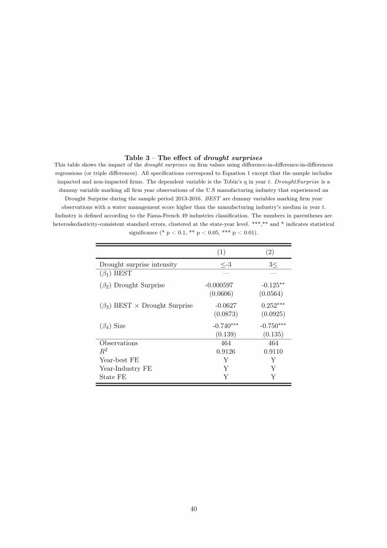
Table 3 – The effect of drought surprisesThis table shows the impact of the drought surprises on firm values using difference-in-difference-in-differencesregressions (or triple differences). All specifications correspond to Equation 1 except that the sample includesimpacted and non-impacted firms. The dependent variable is the Tobin’s q in year t. DroughtSurprise is adummy variable marking all firm year observations of the U.S manufacturing industry that experienced an

Drought Surprise during the sample period 2013-2016. BEST are dummy variables marking firm yearobservations with a water management score higher than the manufacturing industry’s median in year t.

Industry is defined according to the Fama-French 49 industries classification. The numbers in parentheses areheteroskedasticity-consistent standard errors, clustered at the state-year level. ***,** and * indicates statistical

significance (* p < 0.1, ** p < 0.05, *** p < 0.01).

(1) (2)

Drought surprise intensity -3 3(�1) BEST — —

(�2) Drought Surprise -0.000597 -0.125⇤⇤(0.0606) (0.0564)

(�3) BEST ⇥ Drought Surprise -0.0627 0.252⇤⇤⇤(0.0873) (0.0925)

(�4) Size -0.740⇤⇤⇤ -0.750⇤⇤⇤(0.139) (0.135)

Observations 464 464R2 0.9126 0.9110Year-best FE Y YYear-Industry FE Y YState FE Y Y

40

Table

4–

The

econom

icchannels

behin

dw

ater

managem

ent

Thi

sta

ble

show

sth

eim

pact

ofth

edr

ough

tsu

rpri

ses

onse

vera

lfir

m-le

vel

outc

ome

vari

able

sus

ing

diffe

renc

e-in

-diff

eren

ce-in

-diff

eren

ces

regr

essi

ons

(or

trip

ledi

ffere

nces

).T

hede

pend

ent

vari

able

sca

ptur

eth

esu

pply

orde

man

deff

ects

.A

llsp

ecifi

cati

ons

corr

espo

ndto

Equ

atio

n1,

exce

ptth

atI

incl

ude

cale

ndar

quar

ter

fixed

effec

t.T

hesa

mpl

ein

clud

esim

pact

edan

dno

n-im

pact

edfir

ms.

Stan

dard

erro

rsar

ecl

uste

red

atth

est

ate-

year

leve

l.**

*,**

and

*in

dica

tes

stat

isti

cals

igni

fican

ce(*

p<

0.1,

**p

<0.

05,*

**p

<0.

01).

(1)

(2)

(3)

(4)

(5)

(6)

(7)

(8)

SOA

q+1

SOA

q+1

Op.

Ex.

q+1

Op.

Ex.

q+1

CO

GS q

+1

CO

GS q

+1

SGA

q+1

SGA

q+1

Dro

ught

surp

rise

inte

nsity

-3

3

-33

-3

3

-33

(�1)

BE

ST—

——

——

——

—

(�2)

Dro

ught

Surp

rise

0.00

363

-0.0

0663

-0.0

0635

0.01

43⇤⇤

⇤0.

0036

4-0

.004

22-0

.011

6⇤⇤⇤

0.03

37⇤⇤

⇤

(-0.

0051

8)(-

0.00

538)

(-0.

0050

9)(-

0.00

521)

(-0.

0024

8)-(

0.00

392)

-0.0

0439

)(0

.006

51)

(�3)

BE

ST⇥

Dro

ught

Surp

rise

0.00

680.

0072

0.00

878

-0.0

164⇤

⇤0.

0013

6-0

.007

490.

0112

⇤⇤⇤

-0.0

315⇤

⇤⇤

(-0.

0081

6)(-

0.00

633)

(-0.

0072

5)(-

0.00

788)

(-0.

0039

4)(-

0.00

563)

(-0.

0038

6)(0

.006

29)

(�4)

Size

-0.0

521⇤

⇤⇤-0

.053

7⇤⇤⇤

-0.0

237⇤

-0.0

213

0.00

386

-0.0

0638

-0.0

274⇤

⇤⇤-0

.036

1⇤⇤

(-0.

0094

8)(-

0.00

951)

(-0.

0138

)(-

0.01

31)

(-0.

0092

7)(-

0.00

806)

(-0.

0104

)(0

.016

5)

Obs

erva

tion

s19

4519

4519

2919

2918

1211

1117

9811

12Y

ear-

best

FEY

YY

YY

YY

YY

ear-

Indu

stry

FEY

YY

YY

YY

YSt

ate

FEY

YY

YY

YY

YQ

uart

erFE

YY

YY

YY

YY

41

Table 5 – Buy-and-hold abnormal returns (%)

This table reports average and median weekly buy-and-hold abnormal returns (BHARs) around ADV s. BHARsare calculated as the difference between the buy-and-hold returns of the firms with best water managementand the firms with poor water management. The sample period is from 2013 to 2016. The day event windowinclude weeks from 0 to 53 and is denoted [0,53]. N is the number of observations. t-stats are in parenthe-ses. Standard errors are heteroskedasticity-consistent standard errors for median BHARs and are clusteredat the state-year level for average BHARs. *, ** and *** denote significance at the 10%, 5% and 1%, respectively.

Mean Median Observations

(1) [0,53] 16.0⇤⇤ 6.05⇤⇤⇤ 3002(2.46) (3.77)

(2) [-24,0[ 2.57 0.712 1344(0.62) (1.60)

(3) [-12,0[ 1.89 0.0520 672(0.66) (0.09)

(4) [0,24] 5.82 4.01⇤⇤⇤ 1400(1.75) (3.31)

(5) [24,53] 10.9⇤⇤ 8.77⇤⇤⇤ 1658(2.43) (7.81)

(6) ]53,65] 3.48 0.259 2250(-0.60) (0.51)

42

Table 6 – Water Management in the non-manufacturing sector

This table shows the impact of the drought surprises on annual firm values and quarterly operating expenses usingdifference-in-difference-in-differences regressions (or triple differences). All specifications correspond to Equation1 except that the sample includes impacted and non-impacted non-manufaturing firms. The dependent variableis the Tobin’s q in year t or the operating expenses in quarter q+1. DroughtSurprise is a dummy variablemarking all firm year observations of the U.S manufacturing industry that experienced an Drought Surpriseduring the sample period 2013-2016. BEST are dummy variables marking firm year observations with a watermanagement score higher than the manufacturing industry’s median in year t. Industry is defined accordingto the Fama-French 49 industries classification. The numbers in parentheses are heteroskedasticity-consistentstandard errors, clustered at the state-year level. ***,** and * indicates statistical significance (* p < 0.1, ** p< 0.05, *** p < 0.01).

(1) (2) (3) (4)Tobins’ q Tobins’ q Op. Ex.q+1 Op. Ex.q+1

Drought surprise intensity -3 3 -3 3(�1) BEST — — — —

(�2) Drought Surprise 0.0382 0.0333 -0.0108 -0.00219(-0.0357) (0.0311) (-0.0119) (0.0112)

(�3) BEST ⇥ Drought Surprise -0.129⇤⇤ -0.0322 0.013 -0.0123(-0.0625) (0.0376) (-0.0258) (0.0193)

(�4) Size -0.702⇤⇤⇤ -0.709⇤⇤⇤ 0.0231 0.0203(-0.105) (0.107) (-0.0437) (0.0441)

Observations 747 747 2174 2174Best-Year FE Y Y Y YIndustry-Year FE Y Y Y YState FE Y Y Y YQuarter FE N N Y Y

43

Table 7 – What is Water Management ?

This table presents estimates from pooled OLS regressions where the dependent variable is the IVA MSCIwater management score in year t (MGMT ) or in year t + 1 (MGMTt+1) ranging from 0 to 10. MGMT ⇤

corresponds to MGMT but rounded at the nearest integer. Panel A reports estimates using water related itemsfrom Thomson Reuters’s ASSET4. Panel B reports estimates from survey data collected by CDP. CDP Surveyand ASSET4 Data approximately match some MSCI water management metrics in Table 1. Water Withdrawalis the volume of water withdrawal in decameter meters (⇡ 219969 gallons). Water Recycled is the amountof water recycled or reused in decameter meters (⇡ 219969 gallons). WW and WR is the volume of waterwithdrawal and water recycled in cubic meters, respectively. Accidental Spills is the direct and accidental oiland other hydrocarbon spills in thousands of barrels (kbls). Size is the logarithm of the total assets (ln(AT)).All regressions control for year and industry fixed effects. Industry is 8-digit GICS. Standard errors are clusteredat the state-year level. ***,** and * indicates statistical significance (* p < 0.1, ** p < 0.05, *** p < 0.01).

PANEL A: ASSET4 ESG

MGMT MGMT MGMTt+1 MGMT⇤

Water Withdrawal 0.552⇤⇤⇤ 0.381⇤⇤⇤ 0.530⇤⇤⇤ 0.615⇤⇤⇤(0.156) (0.122) (0.150) (0.170)

Water Recycled 0.205 -0.0471 -0.460 0.0799(0.653) (0.736) (0.491) (0.754)

WW/Sales -0.00766⇤⇤⇤ -0.00546⇤⇤⇤ -0.00735⇤⇤⇤ -0.00817⇤⇤⇤(0.00187) (0.00127) (0.00174) (0.00207)

WR/Sales -0.00146 -0.00168 0.00282 -0.000824(0.00503) (0.00607) (0.00504) (0.00556)

WR/WW 0.00634⇤⇤ -0.0624 0.00121 0.00663⇤⇤(0.00276) (0.151) (0.00296) (0.00286)

Accidental Spills -0.0705 -0.0602 -0.120⇤⇤⇤ -0.0813(0.0530) (0.0457) (0.0269) (0.0594)

Size -6.139 -9.872⇤ -5.631 -5.978(5.740) (5.882) (6.225) (6.434)

Size2 0.183 0.292⇤ 0.172 0.176(0.165) (0.169) (0.181) (0.186)

MGMTt�1 0.300⇤⇤⇤(0.0899)

N 134 94 101 134Adj R2 0.401 0.641 0.575 0.375Year FE Y Y Y YIndustry FE Y Y Y Y

PANEL B: CDP

MGMT MGMT MGMTt+1 MGMT⇤

MGMT Integration 0.646 0.748 1.236 0.550(0.477) (0.504) (0.791) (0.483)

Highest Responsibility 0.343⇤⇤ 0.408⇤⇤ 0.265⇤ 0.371⇤⇤⇤(0.134) (0.159) (0.152) (0.136)

Targets 0.872⇤⇤ 1.044⇤⇤⇤ 0.936⇤ 0.912⇤⇤(0.379) (0.381) (0.513) (0.385)

# Penalties -0.0365⇤⇤ -0.0300⇤ 0.00481 -0.0362⇤⇤(0.0171) (0.0176) (0.0181) (0.0172)

Penalties 0.000000260 -0.00000107⇤⇤ -0.000000563 -0.000000246(0.000000511) (0.000000511) (0.000000538) (0.000000545)

Size 0.391 0.291 0.937 -0.0701(1.430) (1.318) (1.576) (1.459)

Size2 -0.00157 -0.0112 -0.0348 0.0181(0.0695) (0.0660) (0.0776) (0.0709)

MGMTt�1 0.382⇤⇤⇤(0.0706)

N 290 188 179 290Adj R2 0.369 0.540 0.417 0.348Year FE Y Y Y YIndustry FE Y Y Y Y

44