does work organisation impact individuals’ labour market...
TRANSCRIPT

MASTER’S THESIS IN ECONOMICS
International Business and Economics Programme
Does Work Organisation Impact Individuals’ Labour Market
Position?
Påverkar arbetsorganisation individers arbetsmarknadsstatus?
Erla Resare Elsa Söderholm
Supervisor: Ali Ahmed
Spring semester 2015 ISRN Number: LIU-IEI-FIL-A--15/02068--SE Department of Management and Engineering (IEI)

English title:
Does Work Organisation Impact Individuals’ Labour Market Position?
Swedish title: Påverkar arbetsorganisation individers arbetsmarknadsstatus?
Authors:
Erla Resare [email protected]
Elsa Söderholm [email protected]
Supervisor: Ali Ahmed
Publication type:
Master’s Thesis in Economics International Business and Economics Programme
Advanced level, 30 credits Spring semester 2015
ISRN Number: LIU-IEI-FIL-A--15/02068--SE
Linköping University Department of Management and Engineering (IEI)
www.liu.se

Abstract
The purpose of this study is to investigate the relationship between work organisation and the
labour market status of employees in Sweden, during the years 2008 to 2012. The main interest
is to analyse the probability of staying employed or not, and staying employed after the general
retirement age.
To assess this relationship three different data sources are combined. Work organisation is
approximated with the NU2012 survey, which was conducted by the Swedish Work
Environment Authority. We use an empirical combination of the questions, and the work
organisation is assumed constant throughout the years. Separate regressions are estimated for
each possible labour market status. The regressions are estimated with cross section models and
random effects panel data models.
We find that there is a relationship between work organisation and employees’ labour market
positions. Numerical flexibility is found to affect the work environment and the individuals’
labour market statuses negatively. Decentralisation’s and learning’s impact on the individuals’
labour market status is, however, incoherent with theories and previous research. These results
are probably due to the reverse time causality of the study. Finally we propose that it is
important to investigate this relationship further to be able to make policy changes.
Keywords: Work organisation, Labour market, Flexibility, Numerical Flexibility,
Decentralisation, Learning, Work environment.

Acknowledgements
We would like to express a sincere thank you to all the people that have helped and guided us
through the process of writing this master’s thesis. First, we would like to thank our supervisor
Ali Ahmed for his encouragement, inspiration, and advice throughout the process. We would
also like to thank Hans-Olof Hagén at Statistics Sweden for his patience and guidance of the
subject. We are utterly grateful for all the rewarding discussions. We are also thankful for the
relevant and interesting inputs from Annette Nylund at The Swedish Work Environment
Authority. Further, this study would not have been possible without the data provided by
Statistics Sweden and The Swedish Work Environment Authority. The study is financed by
Statistics Sweden and the Swedish Work Environment Authority through the project The Good
Work, for which we are appreciative. Last but not least we would like to communicate our
gratitude to our opponent Björn Backgård and our seminar group that have provided great
constructive feedback on our work.
Linköping, June 2015.
Erla Resare Elsa Söderholm

Table of Contents
1. Introduction .................................................................................................................................................... 1 1.1. Significance of This Study ..................................................................................................................................2 1.2. Purpose ......................................................................................................................................................................3 1.3. Method .......................................................................................................................................................................4 1.4. Delimitation .............................................................................................................................................................4 1.5. Contribution to the Research Field ...................................................................................................................5 1.6. Research Ethics .......................................................................................................................................................5
2. Theories and Previous Research .............................................................................................................. 6 2.1. Numerical Flexibility ............................................................................................................................................8 2.2. Functional Flexibility ............................................................................................................................................9
3. Data ................................................................................................................................................................ 13 3.1. The NU2012 Survey........................................................................................................................................... 13 3.2. The LISA Database ............................................................................................................................................ 13 3.3. The Statistical Business Register ................................................................................................................... 14 3.4. Merging the Data Sets ....................................................................................................................................... 14 3.5. Dependent Variables .......................................................................................................................................... 15 3.6. Independent Variables ....................................................................................................................................... 19 3.7. Description of Data ............................................................................................................................................. 21
4. Econometric Method ................................................................................................................................ 25 4.1. Creating a Cross Section Model for the Whole Population ................................................................... 25 4.2. Creating a Cross Section Model Using the NU2012 Survey................................................................. 26 4.3. Panel Data Models .............................................................................................................................................. 27 4.4. Criticism of the Methodology ......................................................................................................................... 28
5. Results and Analysis ................................................................................................................................. 30 5.1. The Cross Section Model.................................................................................................................................. 30 5.2. The Panel Data Model ....................................................................................................................................... 34 5.3. Sensitivity Analysis ............................................................................................................................................ 41
6. Discussion .................................................................................................................................................... 43 6.1. Policy Implications ............................................................................................................................................. 47
7. Conclusions and Further Research ....................................................................................................... 49
References ........................................................................................................................................................ 50
Appendices ....................................................................................................................................................... 55 Appendix A – Description of the Excluded Variables ..................................................................................... 55 Appendix B – Cross Section Results with all Parameters .............................................................................. 57 Appendix C – Panel Data Results with all Parameters .................................................................................... 69

List of Figures FIGURE 1: THE SUBCATEGORIES OF WORK ORGANISATION .........................................................................................................7 FIGURE 2: OVERVIEW OF THE NINE POSSIBLE LABOUR MARKET STATUSES ....................................................................... 16 FIGURE 3: THE COMPOSITION OF THE ELEVEN WORK ORGANISATION PCA COMPONENTS ........................................... 20
List of Tables TABLE 1: SAMPLE SIZE OVER THE YEARS ........................................................................................................................................ 22 TABLE 2: SIZE OF EACH LABOUR MARKET STATUS IN OUR SAMPLE ..................................................................................... 22 TABLE 3: MEAN VALUES OF THE INDIVIDUAL CHARACTERISTICS ........................................................................................... 23 TABLE 4: MEAN VALUES OF THE FIRM SPECIFIC FACTORS OF OUR SAMPLE ....................................................................... 24 TABLE 5: CROSS SECTION RESULTS: MAIN CATEGORIES ........................................................................................................... 30 TABLE 6: CROSS SECTION RESULTS: SUBCATEGORIES OF EMPLOYED ................................................................................... 32 TABLE 7: CROSS SECTION RESULTS: SUBCATEGORIES OF NEGATIVE LABOUR MARKET STATUS ................................ 33 TABLE 8: PANEL DATA RESULTS: MAIN CATEGORIES ................................................................................................................. 35 TABLE 9: PANEL DATA RESULTS: SUBCATEGORIES OF EMPLOYED......................................................................................... 37 TABLE 10: PANEL DATA RESULTS: SUBCATEGORIES OF NEGATIVE LABOUR MARKET STATUS ................................... 39 TABLE 11: A COMPARISON OF THE SIGNIFICANT PANEL DATA RESULTS WITH THE CROSS SECTION RESULTS ....... 41 TABLE 12: CROSS SECTION RESULTS REGARDING EMPLOYED ................................................................................................. 57 TABLE 13: CROSS SECTION RESULTS REGARDING SAME FIRM ................................................................................................ 58 TABLE 14: CROSS SECTION RESULTS REGARDING ANOTHER FIRM ........................................................................................ 59 TABLE 15: CROSS SECTION RESULTS REGARDING NEGATIVE LABOUR MARKET STATUS .............................................. 60 TABLE 16: CROSS SECTION RESULTS REGARDING UNEMPLOYED ........................................................................................... 61 TABLE 17: CROSS SECTION RESULTS REGARDING SICK LEAVE ............................................................................................... 62 TABLE 18: CROSS SECTION RESULTS REGARDING DISABILITY PENSIONER ......................................................................... 63 TABLE 19: CROSS SECTION RESULTS REGARDING OTHER, LOW INCOME ............................................................................ 64 TABLE 20: CROSS SECTION RESULTS REGARDING EMPLOYED AFTER THE AGE OF 65 ..................................................... 65 TABLE 21: CROSS SECTION RESULTS REGARDING EARLY PENSIONER .................................................................................. 66 TABLE 22: CROSS SECTION RESULTS REGARDING STUDENT .................................................................................................... 67 TABLE 23: CROSS SECTION RESULTS REGARDING OTHER, HIGH INCOME............................................................................ 68 TABLE 24: PANEL DATA RESULTS REGARDING EMPLOYED TO SICK LEAVE ....................................................................... 69 TABLE 25: PANEL DATA RESULTS REGARDING DISABILITY PENSIONER TO OTHER, HIGH INCOME ............................ 70

1
1. Introduction
Being out of the labour force is costly for individuals and it may complicate their possibility to
come back to work. Acemoglu (1995) shows that it is difficult for unemployed individuals to
maintain their working skills. Similarly, it is problematic for employers to observe the
individuals’ maintenance of their working skills when they are unemployed and not part of the
working labour force. Therefore employers could discriminate against long-term unemployed
people (Acemoglu, 1995). Work experience is an important signal of productivity for
employers, especially for high skilled jobs and it increases the probability of becoming or
staying employed (Eriksson and Rooth, 2014; Becker, 1980).
It is important to understand how firms affect the workers. In recent years, more focus has been
directed to how work organisation impacts employees and the labour market. Work
organisation is a broad concept but generally it refers to the structure of the firm such as, the
structure of the production process, the relationship between staff and production departments,
the responsibilities at different hierarchical levels, and the design of the job positions
(Eurofound, 2011). Studies show that the type of work organisation has an effect on the health
of the employees and, therefore, also has an effect on their labour market statuses (MEADOW
Consortium, 2010). A good work environment increases the well-being of the employees as
well as lowers the employee turnover. Moreover, it has several other beneficial effects, for
example; higher productivity, motivation among employees, and lower absence rates (Petersson
and Rasmussen, 2013; European Agency for Safety and Health at Work, 2015). Nevertheless,
some studies find that new types of work organisation might have a negative effect on
employees, for example, flexibility can lead to a higher degree of stress and sickness
(Eurofound, 2011).
A large amount of data is needed to evaluate how work organisation impacts individuals. It is
also difficult to measure work organisation since it is a wide concept. To facilitate the measure
of work organisation, the European Commission have developed guidelines, called The
Meadow Guidelines (MEADOW Consortium, 2010). However, few studies have been
conducted on the subject and further research is, therefore, necessary to comprehend the
relationship between work organisation and the labour market.

2
1.1. Significance of This Study
Work organisation appears to affect the employees’ labour market status. The Swedish National
Board for Industrial and Technical Development, NUTEK, (1996) finds that a flexible work
organisation is beneficial for the employees, resulting in lower absence due to sickness and a
lower employee turnover. On the other hand, depending on the method used, Aksberg (2012)
finds contradictory results regarding work organisation’s effect on the probability of becoming
unemployed. With a cross sectional method, decentralisation diminishes the risk of becoming
unemployed, while with a generalised estimating equation method the results are inconclusive.
In addition, Aksberg (2012) tries to evaluate the impact of numerical flexibility and individual
learning with the two different methods but again finds inconsistency in the results. 1
Nevertheless, the research within this area is limited (MEADOW Consortium, 2010).To
strengthen the understanding of how work organisation impacts individuals, further research is
necessary. To be able to draw robust conclusions about the relationship between individuals’
labour market positions and the work organisation, more extensive data is needed. A
disturbance in the labour market has both economic consequences, such as unemployment and
a decreased employability, and consequences in the health, criminality, and the wellbeing of
individuals (Forslund and Nordström Skans, 2007). Further, unhappy or unhealthy individuals
affect the economy since they might be less productive and need more of the society’s
resources. In order for policy makers to create well-functioning regulations, it is necessary to
know all possible impacts. It is therefore important to investigate the economy using as large
sample as possible.
The studies of NUTEK (1996) and Aksberg (2012) both use a theoretical division of work
organisation. The existing theories usually view the work organisation from three different
aspects: flexibility, decentralisation, and learning (Aksberg, 2012; The Swedish Work
Environment Authority, forthcoming). Nevertheless, how firms use work organisation in reality
is rarely represented in the literature. Statistics Sweden (2011) uses an empirical approach when
examining both the effect that it has on individuals and how it affects firms. Another example
that also uses an empirical approach is the study of Petersson and Rasmussen (2013), however,
they investigate the relationship between work organisation and firms’ productivity. In other
words, there is a need to keep studying how work organisation affects individuals using an
empirical perspective.
1 Numerical flexibility is the possibility for the firm to adjust the labour input (Kalleberg, 2001).
3
Previous research has investigated the relationship between work organisation and the Swedish
labour market, during time periods when the Swedish economy was growing (Statistics
Sweden, 2011; Aksberg, 2012). To understand the effects of work organisation, it is important
to examine the effect during all time periods of a business cycle. A labour market that is under
distress due to an economic crisis will react differently to policy changes. Firms use work
organisation to become more productive and increase their competitiveness, something that is
especially important during an economic crisis (Statistics Sweden, 2011; Petersson and
Rasmussen, 2013). As firms use work organisation to survive, it is important to investigate how
it affects the employees during crises. If there is a way for firms to be more flexible that also
benefits the individuals, implementing these work organisation tools would be more
advantageous for the economy.
The Swedish labour force is ageing and it seems probable that the general retirement age will
increase in the future (Bucht, Bylund, and Norlin, 2000; Arbetsgivarverket, 2002; SOU
2013:25). As these individuals are normally not considered a part of the labour force, they are
sometimes excluded from studies of the labour market.2 If work organisation has an effect on
the older employees’ work-life, it is necessary to explore it. The general discussion regards the
regulation of the general retirement age (Motion 2014/15:400). If work organisation affects the
desire to keep working at an older age, it could be used to motivate workers to continue to be a
part of the labour force. In 2011, the Government of Sweden authorised a commission to
examine how to increase the general retirement age. The commission concluded that it is
necessary, and that one solution would be to adjust the work environment (SOU 2013:25). As
with any regulation, there is a need for meticulous studies in this area.
1.2. Purpose
The purpose of this study is to examine how work organisation affects employees’ status in the
Swedish labour market, during the time period 2008 to 2012. Labour market status refers to
different labour market outcomes.3
2 One example of a study that does not include individuals over the age of 65 is the study of Aksberg (2012). 3 For example, working at the same company, working at a different company, becoming unemployed, becoming
a disability pensioner, working after the age of 65 or not belonging to any of the mentioned groups.

4
Research questions
What is the relationship between work organisation and the employees’ labour market
positions?
Specifically, how do numerical flexibility, decentralisation, and learning affect
employees’ labour market status?
How does work organisation affect the probability of working after the general
retirement age?
1.3. Method
We apply econometric methodologies to examine the relationship between work organisation
and labour status of employees. The age of the individuals included range from 16 to 74 years
of age in 2007 and are followed throughout the years 2008 to 2012. Three different data sources
are utilised and combined together. The first set of data comes from the NU2012 survey. The
data is assumed constant over the time period and we use an empirical division of work
organisation. The second set of data comes The Longitudinal Integration Database for Health
Insurance and Labour Market Studies (LISA). And, the third dataset is The Statistical Business
Register (FDB). The regressions are run for each possible labour market outcome separately.
To estimate the impact of work organisation on labour market outcomes we first estimate a
linear probability model using individual data for all Swedish citizens employed in 2007. The
estimated equation is later applied to the individuals of the survey to produce an estimated
variable of the labour market status of the employees. In the final model, a quotient constitutes
the dependent variable and is measured at the company level. To create the quotient, the actual
mean of the work status is divided by the mean of the estimated probability of the work status.
The dependent variable then captures the possible labour market status. The final estimations
of the model are done using two different econometric methods: a cross sectional method and
a random effects panel data method.
1.4. Delimitation
We use the NU2012 survey as a proxy for work organisation. Since the utilised survey was
conducted in 2012 and no further data and information after this year have been collected, the
study goes back five years in time, and therefore starts in 2007. The firms of interest are the
ones that can be traced back to 2007 and that have been active during the whole time period of
this study. To investigate the effect on individuals, we only consider individuals that were
employed in 2007 and follow them until 2012. We investigate the relationship between work

5
organisation and individuals’ labour market status. Other possible impacts on individuals’
labour market positions are not examined in this study.
1.5. Contribution to the Research Field
In contrast to previous studies, this study uses another empirical measure of work organisation.
Previous studies that have used an empirical approach have approximated work organisation
using eight or four components (Petersson and Rasmussen, 2013; Swedish National Board for
Industrial and Technical Development, 1996). This study approximates work organisation
using eleven different components. This is to make the approximation of work organisation
closer to how it used by firms in reality. We also cover a time period that has previously not
been researched within the academia. This provides a wider comprehension on how firms use
work organisation in crises. Moreover, various kinds of possible labour market statuses are
examined. In contrast to previous studies, this study also considers employed individuals older
than the normal retirement age.
1.6. Research Ethics
All data are obtained from various databases at Statistics Sweden and the survey is obtained
from The Swedish Work Environment Authority. The Swedish Work Environment Authority
states that conventional research ethic guidelines have been followed when developing and
conducting the survey (Stelacon, 2013). The data sources at Statistics Sweden and The Swedish
Work Environment Authority are regulated by the Public Access to Information and Secrecy
Act (SFS 2009:400). Regarding personal information about individuals and specific firm data,
these are only used in order to trace the individuals to the firms. Their information is not
presented in accordance with the Swedish Public Access to Information and Secrecy Act (SFS
2009:400). Even though this thesis is financed by Statistics Sweden and the Swedish Work
Environment Authority, the funding is independent of the results and conclusions presented in
the thesis. Moreover the authors of this thesis make their own the decisions and are responsible
for the study’s contents. We acknowledge the Mertonian norms regarding research ethics
(CODEX, 2015).

6
2. Theories and Previous Research
Many existing theories concerning work organisation have emerged from a business point of
view, or from a more humanistic side of organisational structure. In an effort to connect these
theories to general economics, one idea is that both companies and employees are trying to
maximise their benefits. Consequently, an employment contract can end due to two main
problems; the worker is no longer maximising the utility of the firm, or the firm is no longer
maximising the utility of the individual. The theories regard how to maximise firms’ utility of
the employee, hence, they relate to labour economics (Mondy and Mondy, 2014; Lazear and
Oyer, 2012).4
Labour economic theory states that job security and wage have a trade-off relationship; the
more precarious the work is, the higher the salary has to be. This is known as the compensating
wage differential (Björklund et al., 2006). Smith (1964) also emphasises that individuals with
a higher level of human capital are assumed to obtain a higher salary. This idea has developed
into the human capital theory along with the theories of Theodore Schultz and Gary Becker
(Kwon, 2009). In other words, labour market theory does acknowledge that work environment
has an effect on the preferences of the employees, even so, studies regarding work organisation
are dominated by a business perspective.
Another example that examines the work environment and why the individuals are motivated
to work is the motivation-hygiene theory, also called the two-factor theory, by Frederick
Herzberg (Herzberg, Mausner, and Snyderman, 1993). The theory emphasises that for the
individual to be motivated to work, the company needs to provide at least the so-called hygiene
factors. These factors concern, for example, salary, job security, working conditions, company
policy, and firm administration. When these needs have been satisfied, only then the employees
can be encouraged with motivators to develop and become more productive. Achievement,
responsibility, and promotion are counted as motivators, which typically are more directly
connected to the assignment (Bruzelius and Skärvad, 2011). A good work environment is
achieved when the two stages mentioned above are accomplished (Herzberg, Mausner, and
Snyderman, 1993).
Further aspects of the organisational structure are found within the three categories: flexibility,
decentralisation, and learning. Flexibility can be seen as an umbrella category since
4 One field of labour economics that is especially concerned with these practices is personnel economics, yet it
normally excludes the future career of the employees (Lazear and Oyer, 2012).

7
decentralisation and learning are types of functional flexibility (Swedish National Board for
Industrial and Technical Development, 1996). Flexibility is often viewed as beneficial in a
workplace environment, especially for the employees. 5 According to most researchers,
flexibility can be divided into two subgroups, functional and numerical flexibility.6 Functional
and numerical flexibility are, however, also studied in combination. In a report for the OECD,
Tangian (2008) studies if the idea of flexicurity is met in the real world and finds it not being
the case in any of the European countries.7 He studies the relationship between work flexibility
and work precariousness and finds a positive relationship, implying that flexibility increases
the instability of the work for the employees.8 He also examines the flexibility measure:
numerical and functional flexibility, separately.
This study treats numerical and functional flexibility as two separate key categories, where
decentralisation and learning are types of functional flexibility. Figure 1 presents an overview
of the flexibility characteristics.
5 See for example the Society for Human Resource Management (2009). 6 Kalleberg (2001) explains that Atkinson and Smith call it functional and numerical flexibility, meanwhile
Cappelli and Neumark refer to it as internal and external flexibility. 7 Flexibility is often related to the concept of flexicurity which was developed in Denmark (Madsen, 2004). The
idea is that a combination of work flexibility and employment security would be optimal for the labour market and
employability should increase (Tangian, On the European Readiness for Flexicurity: Empirical Evidence with
OECD/HBS Methodologies and Reform Proposals, 2008). 8 The composite indicator of work uncertainty includes questions regarding employability, employment stability,
and income. To assess the relationship he used a combined measure of flexibility, which also included wage
flexibility.
Work Organisation
Flexibility
Functional
Decentralisation
Learning
Structural
Individual
Numerical
External
Internal
Figure 1: The Subcategories of Work Organisation

8
2.1. Numerical Flexibility
Numerical flexibility is the possibility for the firm to adjust the labour input. In
macroeconomics, it is normally argued that numerical flexibility is beneficial for the economy
(Jackman, Layard, and Nickell, 1999). It is often divided into hiring consultants or hiring part-
time employees. Therefore, the numerical flexibility is categorised into external and internal
labour, since firms employ part-time workers internally, while consultants are contracted
externally (Kalleberg, 2001). Internal numerical flexibility has a close theoretical relationship
with unemployment. If employees work fewer hours, the company could hire more people.
Even though this idea has an intuitive explanation, many studies show that the relationship is
not clear-cut and therefore difficult to predict.9 For example, Erbaş and Sayers (2001) discuss
how a reduction in work hours will have a negative first-order effect since the marginal cost of
employing another person is greater than the marginal cost of letting employees work overtime.
Employing another individual could create productivity gains, which constitutes the second-
order effect. This effect might overpower the first-order effect and therefore increase
employment.
Tangian (2008) finds that external flexibility affects employment stability in a negative manner,
yet it has a positive relationship with employability. Further, the internal numerical flexibility
barely affects the employment stability negatively but it has a positive effect on employability.
According to a Swedish study (Aksberg, 2012), a workplace that uses numerical flexibility
increases the probability of becoming unemployed. Furthermore, the study presents a negative
effect during the first four years on the probability of staying employed within the same firm.
Another finding is that the use of numerical flexibility increases the probability of becoming
employed at another firm the first three year of the study and thereafter reduces it. Aksberg
(2012) concludes that the effect of having a flexible work organisation induces employees to
leave their jobs, which constitutes the reason for the positive impact on the probability of being
employed by another firm. Using the same survey as Aksberg (2012), NUTEK (1996) finds a
negative correlation between flexibility and employee turnover. 10 Furthermore they also
encounter that flexibility reduces the amount of sick days utilised by the employees by 24 per
cent.
9 See for example Brunello (1989) and Askenazy (2013). 10 A reduction in the turnover by more than 20 percent, counting turnover as employees being replaced with new
employees (Swedish National Board for Industrial and Technical Development, 1996).

9
2.2. Functional Flexibility
Functional flexibility includes a lot of different factors surrounding the workplace. Kalleberg
(2001, p. 479) defines it as “enhancing employees’ ability to perform a variety of jobs and
participate in decision-making”. This can include decentralisation, organisational learning, job
rotation, the possibility for employees to have a flexible schedule, and the possibility for
employees to decide the working hours by themselves. Decentralisation and learning are treated
separately to be able to draw conclusions on their respective effects and will therefore be
discussed more thoroughly later on in this section. Work task rotation is often considered a
constituting factor of “the good work” through the idea of variation.11 Since individuals are able
to perform different tasks they ought to feel more engaged and motivated to work. Further, the
amount of repetitive strain injuries should diminish (Bruzelius and Skärvad, 2011). Rotation of
work tasks is considered a type of functional flexibility in the workplace since it strengthens
the possibility for the workers to perform different tasks.
Tangian (2008) finds that the use functional flexibility has a positive effect on employment
stability yet constitutes a negative effect on employability. To measure functional flexibility,
Tangian uses questions regarding work task rotation (Tangian, 2007). On the contrary, Huang
(1999) shows that work task rotation enhances employees’ employability through higher
productivity. One reason for the conflicting results could be that they use different populations
for their studies.
2.2.1. Decentralisation
Decentralisation is a well-known concept, yet it has various interpretations. The general
definition of decentralisation is that the decision-making and the political and administrative
power are delegated from a central position in the organisation to a more local level (Pierre,
2001). A decentralised work organisation therefore implies that the employees have more
responsibility, such as quality control, freedom in planning their own work, and often a more
flexible working schedule (Statistics Sweden, 2011).
Decentralised work organisation has in the western world and in the OECD countries often
been seen as something positive. The general idea is that it generates a positive effect on the
work organisation and also enhances democratisation (Greffe, 2003). In order for individuals
to be productive, it is important that they are given the opportunity to develop and take
11 The good work is a broad concept that often involves safety, variety, independency, comprehensive view,
feedback, cooperation, learning and development possibilities. Another closely related work is Corporate Social
Responsibility (Bruzelius and Skärvad, 2011).

10
responsibility. It is necessary that the firm provides the employees information about the tasks
and work organisation in order for them to be motivated and productive. A human being with
information does not bypass taking responsibility (Bruzelius and Skärvad, 2011). The
possibility to work with a flexible schedule leaves larger responsibility yet greater possibilities
for the employee. Thus, the opportunity to decide more about one’s workplace is considered a
motivator according to the theory of Herzberg (Herzberg, Mausner, and Snyderman, 1993).
An empirical study on how work organisation affects individuals’ outcome on the labour market
shows that decentralised work organisations decreases the probability of being unemployed
(Aksberg, 2012). Further, Aksberg (2012) discusses that the reason may be that a decentralised
work organisation encourages employees to take more responsibility. Responsibility is often
seen as an attractive characteristic among employers, of whom these individuals are seen as
more attractive on the labour market. However, the probability that individuals change firm is
lower in a decentralised work organisation (Aksberg, 2012). An explanation is that if the work
organisation is decentralised, individuals are more motivated (Bruzelius and Skärvad, 2011;
Herzberg, Mausner, and Snyderman, 1993). A study from Statistics Sweden (2011) confirms
that a decentralised work organisation tends to have a positive relation to the work environment
and that it lowers the probability to be on sick leave.
Another way to lower the employee absenteeism due to sickness, and to reduce labour turnover,
is through the use of flexitime (Possenriede, Hassink, and Plantenga, 2014).12 A workplace that
allows employees to learn and perform different types of work tasks increases the employees’
health (Lindberg and Vingård, 2001). Lindberg and Vingård (2001) also point out that the
possibility to work with flexible hours is lower for people older than 55 years. In their sample,
43 per cent of the employees below 55 years of age are able to use flexitime, yet the fraction
for employees over the age of 55 is 18 per cent. The implication of this result is that, when
using a combined flexibility index, one has to be careful when evaluating the effect of flexitime
on employees over 55 years of age. On the other hand, Curtis and Moss (1984) do not find any
significant relationship between being on sick leave and applying flexitime.
2.2.2. Structural and Individual Learning
It is important to implement learning within the organisation for a firm to be flexible. Learning
helps the adaption of a rapidly changing environment as well on organisational level as for the
individuals (Statistics Sweden, 2011). Learning within the organisation can be distinguished
12 Flexitime is “a system of working that allows an employee to choose, within limits, the hours for starting and
leaving work each day.” according to dictionary.com.
11
into two parts, structural learning and individual learning. First we describe structural learning
followed by individual learning.
Structural learning refers to the organisational learning, i.e. the knowledge that stays within the
firm (Bruzelius and Skärvad, 2011). Specifically, it is the development of the organisation’s
practices for employees, documentation of work routines, customer satisfaction, and evaluation
of quality control (Petersson and Rasmussen, 2013). Therefore, organisations with high
structural learning will be less dependent on their employees (Statistics Sweden, 2011). A
learning organisation can confront the external effects on the market better and it the work
environment (Bruzelius and Skärvad, 2011). However, even if structural learning is viewed to
have positive effect on the firm, some studies show that it can have a negative effect on the
individuals. Statistics Sweden (2011) finds that structural learning increases the probability to
become retired early.
A learning organisation also involves that the firm enhances a team environment among the
employees, which here refers to performing projects in groups and having team meetings.
Teamwork has recently become an important and central part of work organisation. Employers
seek, to a greater extent, graduates that have good team working skills (Bradshaw, 1989). The
new forms of work organisation require this element and it is an important component for high
performance work organisations. Teamwork can favour greater job autonomy, more
responsibility, and enrich the job satisfaction. Nevertheless teamwork creates higher work
intensity. Thus, this effect may weaken the good work environment (Eurofound, 2007).
Competitive intelligence is a part of structural learning, since it involves investments in the
individuals. Kahaner (1997, p. 16) defines it as “a systematic program for gathering and
analysing information about your competitors’ activities and general business trends to further
your own company’s goals.”. In other words, it is the idea of performing environmental
scanning of the market and its agents to understand and predict changes. The employees’ point
of view is seldom represented in the literature. Nonetheless, they compose an important part of
the company since they accumulate the company’s confidentialities. Fuld and Company is a
firm that specialises in competitive intelligence. They state a directive about not stealing
employees whilst trying to learn a trade secret (Kahaner, 1997). Since the employees have
valuable information regarding the firm, a high personnel turnover will be extra costly for the
company.
The second type of learning is individual learning. Individual learning is related to the human
capital development, which is important for reinforcing individuals’ motivation at work

12
(Petersson and Rasmussen, 2013; Herzberg, Mausner, and Snyderman, 1993). According to
Aksberg’s (2012) study, individual learning within the firm decreases the probability of
becoming unemployed. In contrast to Aksberg’s result, the study of Statistics Sweden (2011)
shows a positive relationship between individual learning and being out of the labour force,
such as unemployed or early retired. Human capital has an important role for economies’
growth, productivity and competitiveness (Barro, 1992). Likewise, on-the-job training in
complement with formal education diminish the unemployment rate and lower the employment
volatility (Cairó and Cajner, 2014). The two aspects, individual learning and structural learning,
are strictly correlated with one another. For the structural learning to be effective it is necessary
to also provide individual learning (Bruzelius and Skärvad, 2011).
13
3. Data
All data used for this thesis were produced and hosted by Statistics Sweden and the Swedish
Work Environment Authority and were drawn from three different databases. The first database
accounted for the work organisation of firms. The second database provided micro data over
the characteristics of the individuals. And the third database was used to control for firm
specific characteristics. All data were processed and analysed using SAS 9.3 and SAS
Enterprise Guide.
3.1. The NU2012 Survey
The NU2012 survey, was a telephone survey that examined organisational structure. It was
conducted during the fall of 2012 by Stelacon for The Swedish Work Environment Authority.
The questions about work organisation were based on the MEADOW guidelines (The Swedish
Work Environment Authority, 2014a; MEADOW Consortium, 2010). The stratified sample
consisted of Swedish companies of various sizes from 21 different industries.13 The smallest
firms had no less than five employees but there was no upper limit. The sample included both
private and public corporations (Stelacon, 2013). The response frequency was around 65 per
cent and according to an error analysis performed by the Swedish Work Environment Authority
(2014b) there were no systematic errors. The municipalities and city councils were the only
ones based on the cfar-number of the workplace and not the Corporate Identity Number (CIN).14
This was due to the fact that municipalities and city councils were registered under one CIN,
even though they included different workplaces.15 Although the survey included 78 questions
about the firm, only question 35 to 77 were of importance for this study. This was because the
answers to these questions concern work organisation, for example, numerical flexibility,
decentralisation, and learning. The complete questionnaire is documented in Stelacon (2013).
The survey was not performed yearly, wherefore we assumed work organisation constant
during our time period.
3.2. The LISA Database
The Longitudinal Integration Database for Health Insurance and Labour Market Studies (LISA)
at Statistics Sweden was used to include data for individual characteristics of the individuals in
our study. The LISA database provided yearly micro data for the whole Swedish population
13 For more information about which industries see Stelacon (2013). 14 The cfar-number is an eight-digit identification number of a workplace used by Statistics Sweden. The CIN is a
Swedish firm identification number, assigned to all firms in Sweden. 15 Municipalities and city councils are the English words for kommuner and landsting, respectively.

14
over the age of 16, for the years 2007 to 2012. The CIN is included in the LISA database and
presents the company at which an individual is employed in November a given year. The rest
of variables used for this study are presented more thoroughly in section 3.6.
3.3. The Statistical Business Register
Information about the firms in this study was drawn from the Statistical Business Register
(FDB) at Statistics Sweden. The FDB is a register that includes all firms in Sweden and their
respective workplaces with yearly firm data. The information in the database ranges from the
CIN, to the number of employees hired by the firm. The data used in this study were for the
years 2007 to 2012, and provided control variables for the final models in this study.
3.4. Merging the Data Sets
The individuals of interest for this study were those that were employed in 2007. The CIN was
used to match individuals to organisations. However, we had to handle companies that had
changed their CIN during the time period. The Company and Workplace Dynamics register
(FAD) is a way to trace companies that change their CIN, using the Labour statistics based on
administrative sources (RAMS). If a majority of the employees is found in the company the
consecutive year, the firm is considered the same as the first year even if the CIN has changed
(Statistics Sweden, 2015a). Through the use of the FAD registry the companies that were no
longer active in 2007 were sorted out and dropped. This procedure was needed due to the
reverse time causality of this study. A firm that was assumed to have the same organisational
structure in 2007, as in 2012, needed to be active throughout our time period. This caused the
number of companies in our sample to decrease from 1,993 companies to 1,387. It was,
however, anticipated that using the FAD registry should be effective since it allows the CIN to
vary over time. The FAD registry was only developed for the CIN, hence the cfar-numbers
were assumed constant. Therefore we dropped a relatively larger share of municipalities and
city council companies, than other companies. Nonetheless, the precision of the information
that was gained by the act of dividing these companies into workplaces was of higher value for
this study.
As the individual data and the work organisation data were merged, one dataset containing the
information about the work organisation and the individual was formed. Thirty companies that
were merged by the cfar-numbers had no workers employed in 2007. These companies were
excluded from the sample, resulting in a sample of 1,357 firms. This was not unexpected since

15
the cfar-numbers were not part of the exclusion of the non-active companies via the FAD
registry.
The individuals included in the final dataset ranged from 16 to 74 years of age in 2007, and
were followed throughout the years 2008 to 2012. Each year there was an upper age limit of 74
years of age, for example, the sample of year 2010 included individuals of 19 to 74 years of
age. This led to a decreasing sample size over the time period. In the sample only working
individuals of the NU2012 survey were included since we needed information regarding their
workplace organisation. Further, only individuals that earned more than 83,000 SEK during
2007 were included. This exclusion of low-earning individuals was done to eliminate workers
that were probably not working in the company during a full year or were only employed for
few hours during the year. Since these individuals were presumed to not have spent a lot of
time at the workplace, they were likely to not be affected by the work organisation. The limit
used was based on a limit that Aksberg (2012) used, which we adjusted for inflation, for
increased comparability. Furthermore, the amount was around two Swedish base amounts,
which is a common income separation in labour economics. The low-earning individuals were
only excluded in 2007. For the rest of the studied years, individuals earning less than the two
base amounts were assigned into a category called Other, Low Income. This was made in order
to analyse the possible effects that work organisation has on low-income earners.
3.5. Dependent Variables
To define the possible outcomes on the labour market, twelve different regressions were
estimated. The main interest of this study was however to examine the probability of staying
employed or entering a negative labour market status. With negative labour market status we
refer to the labour market positions: unemployed, being on sick leave, disability pensioner and
individuals with low declared income. This section presents the dependent variables for these
two regressions and their underlying labour market statuses. The three labour market statuses
that do not regard neither employed nor negative labour market status are presented in
Appendix A. In this section we therefore present nine labour market statuses. The dependent
variable of each regression describes the employees’ possible labour market status.
To classify if the individuals were employed, their declared income needed to be higher than
83,000 SEK yearly. If their income was lower than 83,000 SEK they were classified into a
separate group called Other, Low Income. The base year was 2007 and for the forthcoming
years, until 2012, 83,000×1.02t SEK (where t=1 corresponds to 2008) was used to determine a

16
particular year’s value, where inflation was accounted for. 16 The category Employed is
combined from the two probabilities: working at the same firm as in 2007 and working for
another firm than in 2007.
In recent years it has become more common to work after the general age of retirement. This is
a special case and the individuals older than 65 years of age were, therefore, examined
separately and were not included in the regression called Employed.
If the individuals were no longer employed there were several other possible outcomes. They
could have become unemployed, on long-term sick leave, disability pensioner or still working
but with a declared income lower than 83,000 SEK annually. These four possible outcomes can
be seen as negative outcomes, and were, therefore, first examined together in one regression,
under the name Negative Labour Market Status. Later, to investigate the probability of entering
each possible outcome we made separate regressions of each labour market status. Figure 2
presents an overview of the main categories and their subcategories. The LISA database, which
holds individual information about the citizens of Sweden, was used to create the dependent
variables.
Figure 2: Overview of the Nine Possible Labour Market Statuses
16 The inflation rate is assumed to be two per cent per year, since it is the inflation goal for the Riksbank (2012).
•Same Firm
•Another FirmEmployed
•Unemployed
•Sick Leave
•Disability Pensioner
•Other, Low Income
Negative Labour Market Status
Employed after the Age of 65

17
3.5.1. Employed
One of the main dependent variables of interest was if the individuals are employed. The
variable was created for the individuals that worked at the same firm as in 2007 and the
individuals that had changed firm since the base year 2007. The components of work
organisation can affect the probabilities of staying employed at the same firm and becoming
employed at another firm in opposite directions. A component that has a positive impact on the
individuals’ probability to stay at the same firm should have a negative impact on the
individuals’ probability of becoming employed at a another firm, and vice versa. Later, to get
more precise results, same firm, and another firm were observed in separate regressions.
Same Firm
To define the individuals that were working within the same firm as in 2007, the individuals
from the LISA database were matched with the CIN from the NU2012 survey. To get the firms
from the NU2012 survey we used the FAD registry. The individuals that were traced back to
the same firms as they were registered at in 2007, were identified as working within the same
firm. To define workers, the same income restriction as mentioned before was used.
Another Firm
If the individuals were registered as workers, but at another firm than in 2007, they were
classified as working for another firm. This matching was done with the CIN, using the FAD
registry.
3.5.2. Negative Labour Market Status
The other main category of interest was if the individuals are no longer employed. The
outcomes: Unemployed, Sick Leave, Disability Pensioner and, Other, Low Income, were
merged to form the dependent variable called Negative Labour Market Status. How the four
different negative statuses were created is explained below. Similar to the employed variable,
this dependent variable was split and the negative outcomes were estimated in separate
regressions. This was made in order to get more insights about the effects of each labour market
status.
Unemployed
To identify if individuals were unemployed, the unemployment benefits were used as a
measurement. If the unemployment benefits exceeded at least one third of the yearly total
income of the individual, then the individuals were classified as unemployed. The variables

18
used from the LISA database are called, Arblos, Ampol and Deklon. The restriction was made
in the same way as the study of Aksberg (2012), for increased comparability.17
Sick Leave
The individuals with a number of sick days exceeding 90 days were defined as on Sick Leave.
The number of days used as limit is the minimum set by the Swedish Social Insurance Agency,
to classify a person as on long-term sick leave (Swedish Social Insurance Agency, 2015). The
variable used from the LISA database is called Sjuksum_ndag, which shows the total number
of sick days reported by the employees.
Disability Pensioner
Disability pension is a type of pension that is paid to individuals who are permanently or
temporarily unable to work due to a disability. In contrast to sickness allowance, which people
receive after a certain amount of sick days, disability pension is received due to a disability that
hamper your possibility to work full time during a longer time period. The variable used from
the LISA database is called Fortid, which refers to the amount of money that the individuals
receive as disability pension. No restriction of the amount of received money was made. If the
individuals received any disability pension they were classified as a Disability Pensioner.
Other, Low Income
According to our definition, the workers needed to have a yearly declared income higher than
83,000×1.02t SEK. The employees that had a declared income lower than this limit were
categorised into the category called Other, Low Income. Moreover, the individuals that could
not be included in any of the other categories, were also classified into this variable.
3.5.3. Employed after the Age of 65
As mentioned earlier we were also interested in investigating how work organisation affected
the probability of working after the general age of retirement. The normal age of retirement in
Sweden is 65 years of age, yet it has become more common to continue working after this age
(SOU 2013:25). The individuals within the age span 65 to 74 years were therefore studied
separately. To define the individuals as workers, we used the same income restriction as for the
variable Employed.
17 The restriction was made with the following equation
(𝐴𝑟𝑏𝑙𝑜𝑠+𝐴𝑚𝑝𝑜𝑙)
(𝐴𝑟𝑏𝑙𝑜𝑠+ 𝐴𝑚𝑝𝑜𝑙+𝐷𝑒𝑘𝑙𝑜𝑛>
1
3 .

19
3.6. Independent Variables
To measure work organisation, the responses from the NU2012 survey were used. This study
used an empirical division of the questions to capture how firms use work organisation in
practice. The questions that were used in combination or measured similar practices were
combined into one index. This was obtained using a method called principal component
analysis (PCA). The method analyses the common variance of a number of variables, in this
case the questions from the survey. The variables with a common variance were combined into
a common factor. This method has previously been used in related studies by Nylund (2011)
and Petersson and Rasmussen (2013). The components of our study were based on the
reconstruction made by The Swedish Work Environment Authority (forthcoming). The
difference from previous studies mentioned above, is that the variables Teamwork, Competitive
Intelligence and Flexitime were investigated separately. The mentioned variables were highly
correlated with more than one component, and it was were therefore better to study them
separately. The components used in the analysis of this study are visualised in Figure 3.

20
Figure 3: The Composition of the Eleven Work Organisation PCA Components
Component one and two referred to numerical flexibility. The first component contained
questions regarding the external forms of employment, such as consultants. The second
component, called numerical internal flexibility, regarded questions about part-time workers
and employees with temporary contracts.
Component 3 to component 11 referred to functional flexibility. The third component referred
to rotation of work tasks and was constructed from one question only. The next three
components included information concerning decentralisation. Component four observed the
decentralised planning, which contained responsibility for the weekly and daily planning and
responsibility for customer relations. The fifth component reflected decentralised quality
control, which was mainly about responsibility for daily control, follow up and evaluation of
Work Organisation Components
• Q.37 Employees from employment agencies
• Q.38 Share of consultantsComponent 1: Numerical external flexibility
• Q.35 Employees with temporary contracts
• Q.36 Share of part-time workersComponent 2: Numerical internal flexibility
• Q.67 Rotation of work tasksComponent 3: Rotation of work tasks
• Q.46 Responsibility for daily planning
• Q.47 Responsibility for weekly planning
• Q.48 Responsibility for customer relationsComponent 4: Decentralised planning
• Q.49 Purchasing of material for daily work
• Q.50 Follow up and evaluation of work
• Q.51 Responsibility for daily quality controlComponent 5: Decentralised quality control
• Q.57 Employees with flexible work hoursComponent 6: Flexitime
• Q.59 Evaluation of quality in production
• Q.60 Documentation of work routines
• Q.62 Measurement of customer satisfactionComponent 7: Follow-up
• Q.61 Enviornmental scanning
• Q.69 Employees with yearly appraisals
• Q.70 Promotion connected to appraisalsComponent 8: Individual evaluation
• Q.53 Engagement in projects or groups
• Q.55 Involvement in improvement projects
• Q.56 Frequency of team meetingsComponent 9: Teamwork
• Q.65 Formal competence developmentComponent 10: Comptetitve intelligence
• Q.63 Education on paid work hours
• Q.66 Employees with on-the-job-training.
• Q.71 Performance based salary
• Q.64 Unpaid leave for educational purposes
Component 11: Individual learning

21
work, and purchase of material for daily work. Component six referred to one question only,
which asked about flexible work hours.
Component seven, eight, nine and ten conducted information about the structural learning
within the firm. The seventh component considered documentation of work routines, measuring
of customer satisfaction, and quality evaluation in production. Component eight denoted
individual evaluation, which referred to if firms used yearly feedback for their employees. The
ninth component covered mainly the activity that the employees did in groups, for example,
teamwork activities that the firm offered. The tenth component referred to competitive
intelligence at the firm. The last component revealed the individual learning and the human
capital development at the firm. It consisted of questions about the personnel education and the
competence development.
Firm and individual characteristics were used as control variables.18 The variables related to the
firm were type of industry and number of workers at the firm. The variable for type of industry
was assembled from The Swedish Work Environment Authority’s study (forthcoming).
Number of workers was taken from the FDB. Variables regarding the economic performance
of the firms were not included since they are unavailable for public companies. Moreover, this
information was absent for many of the firms included in our study. The individual
characteristics were: age, gender, profession, children, ethnicity, and region. For these
characteristics we created dummy variables.
3.7. Description of Data
This sample only included the individuals that were employed in 2007. Table 1 shows the
number of individuals for our sample, throughout our time period. It is noteworthy that the
number decreases with time. This is because no individuals were added after the year of 2007.
As time passed, some individuals deceased or moved abroad, which explains the decreasing
sample size.
18 The included control variables are common as explanation or control variables in the science of labour
economics.
22
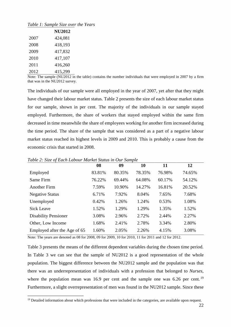
Table 1: Sample Size over the Years
NU2012
2007 424,081
2008 418,193
2009 417,832
2010 417,107
2011 416,260
2012 415,299 Note: The sample (NU2012 in the table) contains the number individuals that were employed in 2007 by a firm
that was in the NU2012 survey.
The individuals of our sample were all employed in the year of 2007, yet after that they might
have changed their labour market status. Table 2 presents the size of each labour market status
for our sample, shown in per cent. The majority of the individuals in our sample stayed
employed. Furthermore, the share of workers that stayed employed within the same firm
decreased in time meanwhile the share of employees working for another firm increased during
the time period. The share of the sample that was considered as a part of a negative labour
market status reached its highest levels in 2009 and 2010. This is probably a cause from the
economic crisis that started in 2008.
Table 2: Size of Each Labour Market Status in Our Sample 08 09 10 11 12
Employed 83.81% 80.35% 78.35% 76.98% 74.65%
Same Firm 76.22% 69.44% 64.08% 60.17% 54.12%
Another Firm 7.59% 10.90% 14.27% 16.81% 20.52%
Negative Status 6.71% 7.92% 8.04% 7.65% 7.68%
Unemployed 0.42% 1.26% 1.24% 0.53% 1.08%
Sick Leave 1.52% 1.29% 1.29% 1.35% 1.52%
Disability Pensioner 3.08% 2.96% 2.72% 2.44% 2.27%
Other, Low Income 1.68% 2.41% 2.78% 3.34% 2.80%
Employed after the Age of 65 1.60% 2.05% 2.26% 4.15% 3.08%
Note: The years are denoted as 08 for 2008, 09 for 2009, 10 for 2010, 11 for 2011 and 12 for 2012.
Table 3 presents the means of the different dependent variables during the chosen time period.
In Table 3 we can see that the sample of NU2012 is a good representation of the whole
population. The biggest difference between the NU2012 sample and the population was that
there was an underrepresentation of individuals with a profession that belonged to Nurses,
where the population mean was 16.9 per cent and the sample one was 6.26 per cent. 19
Furthermore, a slight overrepresentation of men was found in the NU2012 sample. Since these
19 Detailed information about which professions that were included in the categories, are available upon request.

23
variables were control variables, the overrepresentation of certain groups should not
systematically change our results.
Table 3: Mean Values of the Individual Characteristics
Population NU2012 Population NU2012
Age Kids
16 - 34 22.72% 19.90% No kids 34.95% 37.72%
35 - 54 49.40% 50.70% Kids 0 – 6 years 18.86% 17.57%
55 - 64 21.71% 23.99% Kids 7 – 15 years 22.21% 21.26%
65 - 74 6.17% 5.40% Kids >15 years 23.97% 23.44%
Education Background
Compulsory School 12.36% 11.26% Swedish 86.16% 86.62%
Upper Sec. School 48.87% 46.96% Western 3.96% 4.05%
Higher Education 38.77% 41.78% Other 7.25% 6.82%
Occupation Region
Managers 6.65% 6.07% Stockholm 26.08% 28.43%
High Skill 33.52% 42.40% Big City 22.24% 18.52%
Priests 0.14% 0.01% Larger Reg C 37.31% 41.04%
Operators 7.47% 7.63% Smaller Reg C 10.80% 8.91%
Drivers 5.55% 6.97% Small Reg Private 2.24% 2.20%
Nurses 16.90% 6.26% Small Reg Public 1.30% 1.14%
Low Skill 20.02% 22.23%
Artisan 9.77% 8.18%
Gender
Male 51.65% 56.85%
Female 48.35% 43.15%
Note: The population is all the individuals that were employed in 2007. The NU2012 refers to our sample. All the
percentages are means of the shares throughout the time period. Upper Sec. School refers to Upper Secondary
School. The classification regarding occupation was made on the basis of our data and Statistics Sweden’s division
of occupational group called SSYK (Statistics Sweden, 2015b). Our division of the occupations are available upon
request. The background categorisation refers to the birth country. Western refers to North America, The Nordic
countries (except Sweden), EU15 and Oceania. Other refers to the countries that are not part of the classification
Western or Swedish.
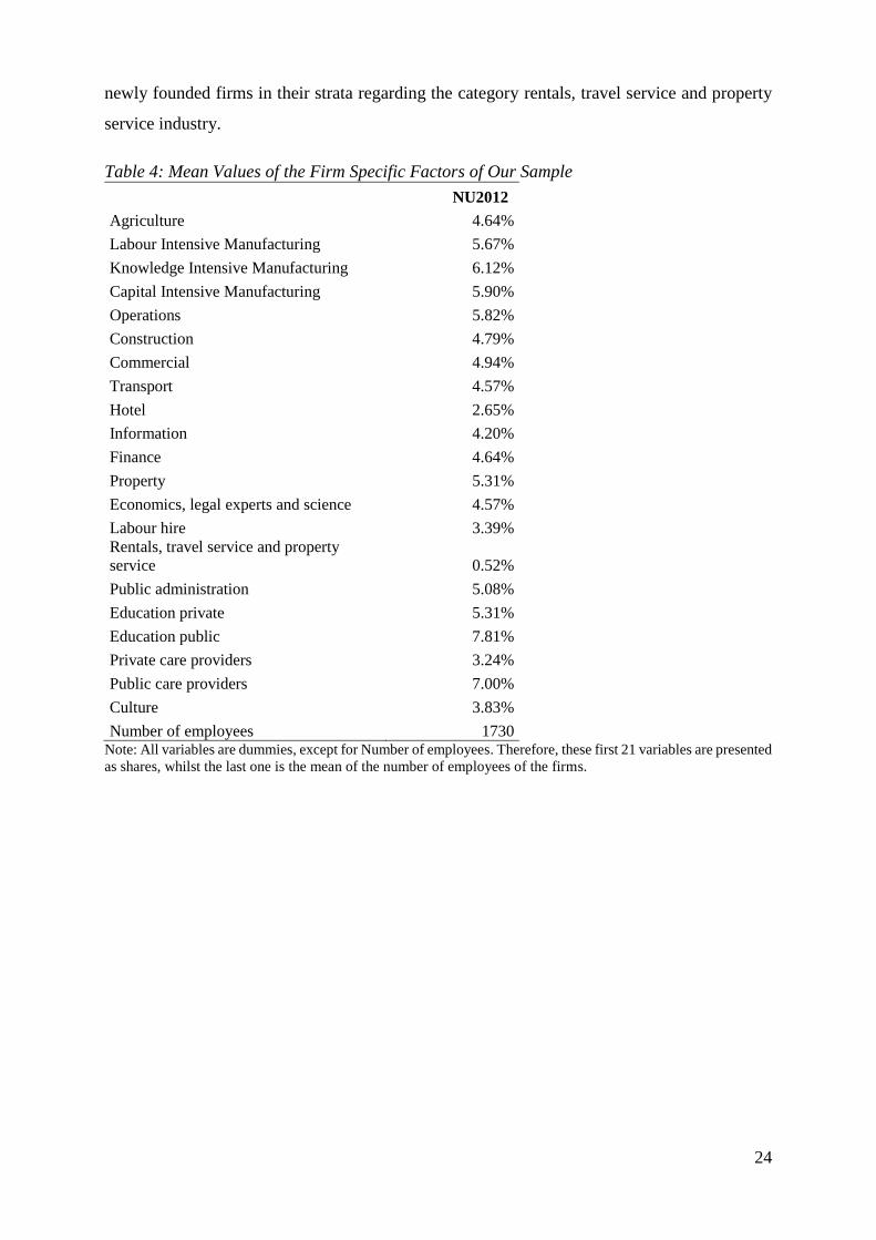
Table 4 shows the industry composition of the NU2012 sample and the mean of the number of
employees in the sample. Since the sample was stratified, the industries were more or less
equally represented in the sample. The industry that had the highest representation was public
care providers, representing seven per cent of the sample. The industry, which included rentals,
travel service and property service, represented only 0.52 per cent of the sample. Assessing the
response rate shown in the technical report of the survey, it was noted that this industry had a
different response level in comparison to ours, presented in Table 4 (Stelacon, 2013). An
explanation is that, in our survey we excluded the firms that were inactive throughout the years
2007 to 2012. Since the survey was conducted in 2012 it can, however, include firms that have
been established after the year of 2007. It could therefore be that the survey included many
24
newly founded firms in their strata regarding the category rentals, travel service and property
service industry.
Table 4: Mean Values of the Firm Specific Factors of Our Sample NU2012
Agriculture 4.64%
Labour Intensive Manufacturing 5.67%
Knowledge Intensive Manufacturing 6.12%
Capital Intensive Manufacturing 5.90%
Operations 5.82%
Construction 4.79%
Commercial 4.94%
Transport 4.57%
Hotel 2.65%
Information 4.20%
Finance 4.64%
Property 5.31%
Economics, legal experts and science 4.57%
Labour hire 3.39%
Rentals, travel service and property
service 0.52%
Public administration 5.08%
Education private 5.31%
Education public 7.81%
Private care providers 3.24%
Public care providers 7.00%
Culture 3.83%
Number of employees 1730 Note: All variables are dummies, except for Number of employees. Therefore, these first 21 variables are presented
as shares, whilst the last one is the mean of the number of employees of the firms.

25
4. Econometric Method
The individuals that were employed in the year of 2007 were followed through the years 2008
to 2012. First we estimated a cross section model using the whole population that was employed
in 2007. This assured that our sample was a good representation of the whole population.
Secondly the effect of work organisation on our sample was estimated using both cross section
and panel data models. The explanatory variables of the two different models were the same.
4.1. Creating a Cross Section Model for the Whole Population
Different individuals have different labour market prospects. It was therefore a need to control
for individual characteristics when estimating the probability of entering each labour market
status. We calculated an estimated value of the labour market positions for each firm, using
data from the whole population. If our sample was not a perfect representation of the population,
this technique would improve the robustness of our estimations.
A linear probability model (LPM) was estimated using individual data of all employed
individuals of 2007. In order to compare the population to the sample, all labour market statuses
were coded equally and data were processed the same way as when the sample of individuals
employed at NU2012 firms was created. Hence, the dataset only included individuals that were
employed in the year of 2007, earning more than 83,000 SEK during that year. The estimations
were made with a year-wise OLS for each labour market status. To control for individual
characteristics, various dummy variables were included. The equation
𝑦𝑖 = 𝛼0 + 𝛼1𝐴𝑔𝑒 + 𝛼2𝐺𝑒𝑛𝑑𝑒𝑟 + 𝛼3𝑃𝑟𝑜𝑓𝑒𝑠𝑠𝑖𝑜𝑛 + 𝛼4𝐶ℎ𝑖𝑙𝑑𝑟𝑒𝑛 + 𝛼5𝐸𝑡ℎ𝑛𝑖𝑐𝑖𝑡𝑦 + 𝛼6𝑅𝑒𝑔𝑖𝑜𝑛 + 𝜀𝑖
[Eq1]
was estimated for all the different labour market outcomes separately. Therefore yi took the
form of the twelve different probabilities for each individual, i, since there were twelve different
labour market outcomes.20 Even though some variables were not statistically significant in
some of our models, they were still kept throughout all models for consistency. This was also
due to the theoretical justification of the model and because the variables included have been
proven to empirically affect the labour market outcomes.
As a model was estimated for the probability of the presence of each labour market status,
twelve different models were estimated for each year. Using all the models, a prediction of the
20 The results from these regressions are available upon request.
26
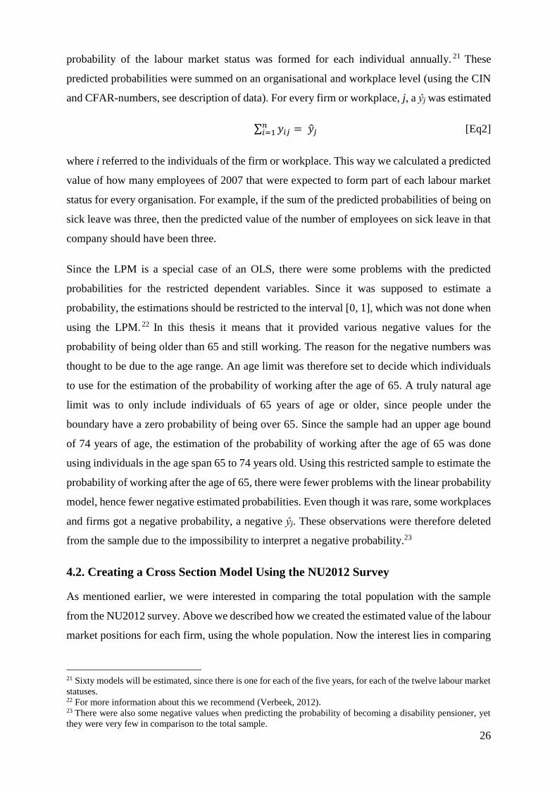
probability of the labour market status was formed for each individual annually. 21 These
predicted probabilities were summed on an organisational and workplace level (using the CIN
and CFAR-numbers, see description of data). For every firm or workplace, j, a ŷj was estimated
∑ 𝑦𝑖𝑗 = �̂�𝑗𝑛𝑖=1 [Eq2]
where i referred to the individuals of the firm or workplace. This way we calculated a predicted
value of how many employees of 2007 that were expected to form part of each labour market
status for every organisation. For example, if the sum of the predicted probabilities of being on
sick leave was three, then the predicted value of the number of employees on sick leave in that
company should have been three.
Since the LPM is a special case of an OLS, there were some problems with the predicted
probabilities for the restricted dependent variables. Since it was supposed to estimate a
probability, the estimations should be restricted to the interval [0, 1], which was not done when
using the LPM. 22 In this thesis it means that it provided various negative values for the
probability of being older than 65 and still working. The reason for the negative numbers was
thought to be due to the age range. An age limit was therefore set to decide which individuals
to use for the estimation of the probability of working after the age of 65. A truly natural age
limit was to only include individuals of 65 years of age or older, since people under the
boundary have a zero probability of being over 65. Since the sample had an upper age bound
of 74 years of age, the estimation of the probability of working after the age of 65 was done
using individuals in the age span 65 to 74 years old. Using this restricted sample to estimate the
probability of working after the age of 65, there were fewer problems with the linear probability
model, hence fewer negative estimated probabilities. Even though it was rare, some workplaces
and firms got a negative probability, a negative ŷj. These observations were therefore deleted
from the sample due to the impossibility to interpret a negative probability.23
4.2. Creating a Cross Section Model Using the NU2012 Survey
As mentioned earlier, we were interested in comparing the total population with the sample
from the NU2012 survey. Above we described how we created the estimated value of the labour
market positions for each firm, using the whole population. Now the interest lies in comparing
21 Sixty models will be estimated, since there is one for each of the five years, for each of the twelve labour market
statuses. 22 For more information about this we recommend (Verbeek, 2012). 23 There were also some negative values when predicting the probability of becoming a disability pensioner, yet
they were very few in comparison to the total sample.
27
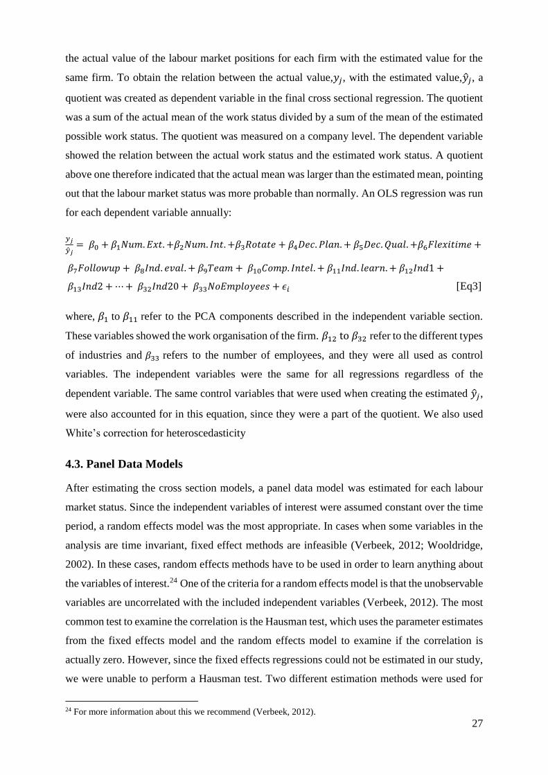
the actual value of the labour market positions for each firm with the estimated value for the
same firm. To obtain the relation between the actual value,𝑦𝑗, with the estimated value,�̂�𝑗, a
quotient was created as dependent variable in the final cross sectional regression. The quotient
was a sum of the actual mean of the work status divided by a sum of the mean of the estimated
possible work status. The quotient was measured on a company level. The dependent variable
showed the relation between the actual work status and the estimated work status. A quotient
above one therefore indicated that the actual mean was larger than the estimated mean, pointing
out that the labour market status was more probable than normally. An OLS regression was run
for each dependent variable annually:
𝑦𝑗
�̂�𝑗= 𝛽0 + 𝛽1𝑁𝑢𝑚. 𝐸𝑥𝑡. +𝛽2𝑁𝑢𝑚. 𝐼𝑛𝑡. +𝛽3𝑅𝑜𝑡𝑎𝑡𝑒 + 𝛽4𝐷𝑒𝑐. 𝑃𝑙𝑎𝑛. + 𝛽5𝐷𝑒𝑐. 𝑄𝑢𝑎𝑙. +𝛽6𝐹𝑙𝑒𝑥𝑖𝑡𝑖𝑚𝑒 +
𝛽7𝐹𝑜𝑙𝑙𝑜𝑤𝑢𝑝 + 𝛽8𝐼𝑛𝑑. 𝑒𝑣𝑎𝑙. + 𝛽9𝑇𝑒𝑎𝑚 + 𝛽10𝐶𝑜𝑚𝑝. 𝐼𝑛𝑡𝑒𝑙. + 𝛽11𝐼𝑛𝑑. 𝑙𝑒𝑎𝑟𝑛. + 𝛽12𝐼𝑛𝑑1 +
𝛽13𝐼𝑛𝑑2 + ⋯ + 𝛽32𝐼𝑛𝑑20 + 𝛽33𝑁𝑜𝐸𝑚𝑝𝑙𝑜𝑦𝑒𝑒𝑠 + 𝜖𝑖 [Eq3]
where, 𝛽1 to 𝛽11 refer to the PCA components described in the independent variable section.
These variables showed the work organisation of the firm. 𝛽12 to 𝛽32 refer to the different types
of industries and 𝛽33 refers to the number of employees, and they were all used as control
variables. The independent variables were the same for all regressions regardless of the
dependent variable. The same control variables that were used when creating the estimated �̂�𝑗,
were also accounted for in this equation, since they were a part of the quotient. We also used
White’s correction for heteroscedasticity
4.3. Panel Data Models
After estimating the cross section models, a panel data model was estimated for each labour
market status. Since the independent variables of interest were assumed constant over the time
period, a random effects model was the most appropriate. In cases when some variables in the
analysis are time invariant, fixed effect methods are infeasible (Verbeek, 2012; Wooldridge,
2002). In these cases, random effects methods have to be used in order to learn anything about
the variables of interest.24 One of the criteria for a random effects model is that the unobservable
variables are uncorrelated with the included independent variables (Verbeek, 2012). The most
common test to examine the correlation is the Hausman test, which uses the parameter estimates
from the fixed effects model and the random effects model to examine if the correlation is
actually zero. However, since the fixed effects regressions could not be estimated in our study,
we were unable to perform a Hausman test. Two different estimation methods were used for
24 For more information about this we recommend (Verbeek, 2012).

28
the random effects estimation; the Fuller and Battese’s method and the Wansbeek and
Kapteyn’s method. The former is used for balanced data and the latter for unbalanced data. SAS
9.3 uses these methods as default for balanced and unbalanced data, respectively (SAS Institute
Inc., 2015). The unbalanced data was due to the exclusion of estimations of probabilities that
were negative. To correct the standard error for possible heteroscedasticity, we applied the
Arellano (1987) correction.
4.4. Criticism of the Methodology
To create the components, questions from the NU2012 survey were used. The questions were
assembled into indices. The questions that firms used in combination or the ones that measured
similar work tasks formed one component, this was done with a PCA analysis. The problem
with indices is that one cannot interpret the magnitude of the estimated regressors. If another
approach would have been used it would have been interesting to investigate which work
organisation measures have greater impacts.
The reverse time causality of this study could have proposed a problem with finding significant
results. Since the NU2012 survey was performed in 2012, the work organisation of the firms
had to be assumed constant throughout the studied time period. This method has previously
been used by Statistics Sweden (2011) when examining work organisation. They included
questions about how work organisation had changed during the last three years and concluded
that work organisation could be assumed constant throughout their time period. Based on this
finding, the reverse time causality of this thesis should not have created unreliable results.
However, the time period 2007 to 2012 could be considered a more extreme one than 2005 to
2008, due to the economic crisis of 2008. Some studies have shown that the crisis has had an
effect on work organisation, for example firing agency staff in Germany (Bispinck, Dribbusch,
and Öz, 2010), providing less flexible work arrangements in the US (Sweet et al., 2014) and
restructures of the firm in the EU27 (Eurofound, 2012). Further, Eurofound (2012) presents that
Sweden and Finland are the countries with most restructuring following the crisis, among the
EU27 member states. Hence the reverse time causality could have inhibited the possibility to
assume work organisation components constant.
The selected time period was heavily affected by the crisis of 2008. Therefore the results from
this study might not be applicable in another time period. As explained previously, an economic
recession has a negative impact on employment and if one were to test our method on data from
another time period, the results could differ.

29
The first regressions were made on the whole population to estimate the probabilities of
entering each labour market status using a linear probability model. The biggest flaws of the
linear probability model are that its estimates are not limited to the interval [0, 1] and that it
assumes the probability increases linearly (Stock and Watson, 2011). The firms for whom the
aggregated estimated probabilities were below zero for each labour market status had to be
removed. Even though there were few firms excluded in this process, using a logit or a probit
model could have solved the issue. The downsides of a LPM were however small for our
method. This was because we did not interpret the probabilities of the first model, i.e. the LPM.
This study aims to examine the relationship between work organisation and the quotient of the
possible labour market outcomes. The probabilities as absolute numbers were therefore not
analysed.
The study was also limited to investigating the effect that the firms have on people that were
already employed. Nonetheless, it could have been that providing certain work organisation
traits would change non-employed individuals’ preferences. Further, there are two parts of an
employment contract, the firm and the employee. This thesis did not distinguish between the
two affecting channels, something that could have provided a more nuanced presentation of the
issue.

30
5. Results and Analysis
This section explains and analyses the results from the two different econometric methods. The
results from the cross section models are presented first, followed by the estimations from the
panel data models. Lastly, we compare and investigate the results obtained from the two
different methods. Since the independent variables of interest, i.e., the eleven components were
indices, the interest lies in the signs of the estimated parameters (plus or minus). We focus on
analysing the statistically significant results, with the highest significance level being ten per
cent.
5.1. The Cross Section Model
This section presents the significant results of the components’ positive and negative impacts.
The regressors found significant in the cross section regressions are marked with a plus sign
(+) if the regressor had a positive sign, and a minus sign (–) if the regressor was negative and
statistically significant at ten per cent level, or less. First we present the results regarding the
main categories, Employed, Negative Labour Market Status and Employed after the Age of 65.
Thereafter, we present the results regarding the more specific outcomes for the category
Employed: Same Firm and Another Firm. Lastly we discuss the results regarding the more
specific outcomes under the category Negative Status: Unemployed, Sick leave, Disability
Pensioner, and Other Low Income. The estimated parameters for all regressions are accessible
in Tables 12 to 23 in Appendix B.
Table 5: Cross Section Results: Main Categories Employed Negative Status Employed after the Age of 65 08 09 10 11 12 08 09 10 11 12 08 09 10 11 12
Num. Ext. + + – – – – – – – – Num. Int. – + + + + + – – – – Rotate – – + Dec. Plan. – – + – – – – – Dec. Qual. + + + Flexitime – Follow-up + – – – – – – Ind. Eval. – – – – Team + + Comp.Intel. + + Ind. Learn. Note: The years are denoted as 08 for 2008, 09 for 2009, 10 for 2010, 11 for 2011 and 12 for 2012. The plus sign
indicates that the explanatory variable has a positive impact on the dependent variables, whereas, the minus sign
denotes a negative effect on the dependent variable. The regression also includes firm characteristics that were
used as control variables.
31
Table 5 displays the statistically significant results from the three main categories of the
possible outcomes on the labour market. The statistically significant results from the first cross
section model, estimated with the employed quotient as the dependent variable, are represented
under the column called Employed. The category Employed included individuals that still
worked at the same firm as in 2007, and the ones that worked for another firm. A work
organisation that is perceived as good by the employees should make them want to stay, hence
they would not want to leave. The components that had a positive impact on the probability of
staying at the same firm decreased the probability of working for a another firm. The work
organisation therefore had ambiguous influence on the variable Employed. As observed, there
were no clear-cut results. Decentralised planning, Dec.Plan, had a negative relationship with
the probability of staying employed. Work task rotation, Rotate, had a significant negative
effect during two years on the probability of staying employed. Numerical external flexibility,
Num.Ext, had a positive effect on the probability during two years, 2010 and 2012. However, it
is essential to notice that this study did not examine the effect that the work organisation had
on the externally employed personnel. This was because these employees were registered under
the leasing firms’ CIN. The individuals that were employed internally, however, were registered
under the firm’s CIN. Furthermore, in Table 5 additional significant results can be found, yet
they are irregular.25
The second main outcome on the labour market is the one called Negative Status in Table 5.
Numerical internal flexibility, Num.Int, was statistically significant and positive during all the
studied years. Moreover, numerical external flexibility was found negative during the last three
years. Aside from these effects, the statistically significant results were irregular. As for the
labour market status Employed, Negative Status was a combined category of four possible
negative labour market outcomes. Due to this, if the work organisation had diverse effects on
the different negative labour market statuses, it would have had an ambiguous effect on this
probability.
The regression regarding staying employed after the age of 65 is presented last in Table 5.
Numerical external flexibility, decentralised planning, and follow-up, Follow-Up, all showed
negative relationships with the probability throughout the years. Additionally, numerical
internal flexibility and individual evaluation, Ind.Eval, showed negative effects during four
years. Teamwork, Team, had a positive effect during three years, as had decentralised quality
control, Dec.Qual. The rest of the results were irregular.
25 The use of irregular and occasional in this section refers to that the effect is significant during only one year.

32
Table 6: Cross Section Results: Subcategories of Employed Employed
Same Firm Another Firm
08 09 10 11 12 08 09 10 11 12
Num. Ext. – + + + +
Num.Int. – + Rotate – Dec. Plan. – – – – Dec. Qual. Flexitime + Follow-up + Ind. Eval. – + + Team Comp.Intel – Ind. Learn.
Note: The years are denoted as 08 for 2008, 09 for 2009, 10 for 2010, 11 for 2011 and 12 for 2012. The plus sign
indicates that the explanatory variable has a positive impact on the dependent variables, whereas, the minus sign
denotes a negative effect on the dependent variable. The regression also includes firm characteristics that were
used as control variables.
Table 6 demonstrates the results considering the two parts of the category Employed: staying
employed at same firm as in 2007 and working for another firm than in 2007. The results for
the probability of staying employed at the same firm were mainly irregular. The only sequent
and statistically significant results were found for decentralised planning, which had a negative
effect. For the probability of becoming employed at another firm, two of the work organisation
components, numerical external flexibility and individual evaluation, showed a statistical
significant impact on the probability. Both components had a positive impact on the probability
of becoming employed at another firm. The rest of the results observed in Table 6 are mostly
irregular.
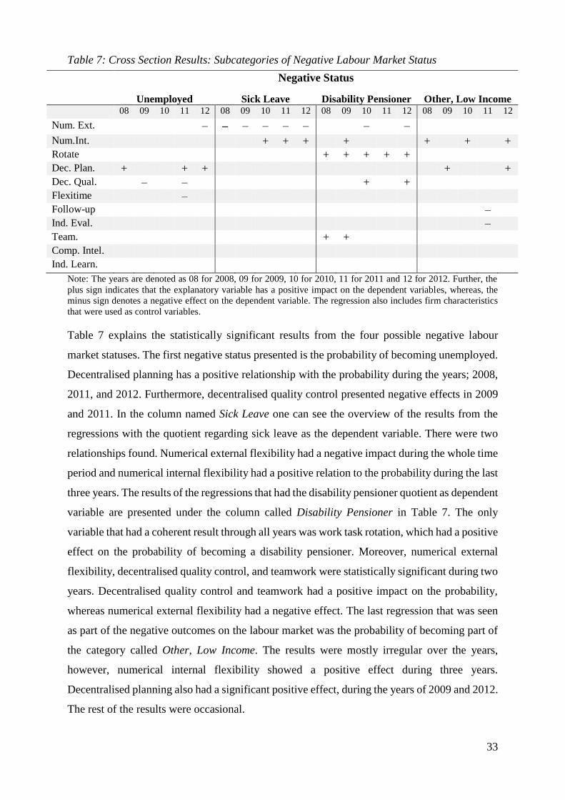
33
Table 7: Cross Section Results: Subcategories of Negative Labour Market Status
Note: The years are denoted as 08 for 2008, 09 for 2009, 10 for 2010, 11 for 2011 and 12 for 2012. Further, the
plus sign indicates that the explanatory variable has a positive impact on the dependent variables, whereas, the
minus sign denotes a negative effect on the dependent variable. The regression also includes firm characteristics
that were used as control variables.
Table 7 explains the statistically significant results from the four possible negative labour
market statuses. The first negative status presented is the probability of becoming unemployed.
Decentralised planning has a positive relationship with the probability during the years; 2008,
2011, and 2012. Furthermore, decentralised quality control presented negative effects in 2009
and 2011. In the column named Sick Leave one can see the overview of the results from the
regressions with the quotient regarding sick leave as the dependent variable. There were two
relationships found. Numerical external flexibility had a negative impact during the whole time
period and numerical internal flexibility had a positive relation to the probability during the last
three years. The results of the regressions that had the disability pensioner quotient as dependent
variable are presented under the column called Disability Pensioner in Table 7. The only
variable that had a coherent result through all years was work task rotation, which had a positive
effect on the probability of becoming a disability pensioner. Moreover, numerical external
flexibility, decentralised quality control, and teamwork were statistically significant during two
years. Decentralised quality control and teamwork had a positive impact on the probability,
whereas numerical external flexibility had a negative effect. The last regression that was seen
as part of the negative outcomes on the labour market was the probability of becoming part of
the category called Other, Low Income. The results were mostly irregular over the years,
however, numerical internal flexibility showed a positive effect during three years.
Decentralised planning also had a significant positive effect, during the years of 2009 and 2012.
The rest of the results were occasional.
Negative Status
Unemployed Sick Leave Disability Pensioner Other, Low Income 08 09 10 11 12 08 09 10 11 12 08 09 10 11 12 08 09 10 11 12
Num. Ext. – – – – – – – – Num.Int. + + + + + + + Rotate + + + + + Dec. Plan. + + + + +
Dec. Qual. – – + + Flexitime – Follow-up – Ind. Eval. – Team. + + Comp. Intel. Ind. Learn.

34
5.2. The Panel Data Model
The results are described in the same way as for the cross section results. First the results
regarding the labour market statuses: Employed, Negative Status, and Employed after the Age
of 65, are presented. Second, we present the results from the regressions regarding Same Firm
and Another Firm. Lastly, the negative statuses are analysed. We only present the explanatory
variables, since they are the ones of interest. All estimated parameters are presented in Tables
24 to 25 in Appendix C. Finally, we compare and investigate the results obtained from the two
different econometric methods.

35
Table 8: Panel Data Results: Main Categories Employed Negative Status Over 65
Intercept 1.090*** 0.733*** 0.236*** (0.022) (0.090) (0.030)
Num.Ext. 0.027** -0.272*** -0.089*** (0.014) (0.069) (0.016)
Num.Int. -0.042** 0.311*** -0.072** (0.021) (0.088) (0.029)
Rotate -0.012* 0.032 -0.007 (0.006) (0.028) (0.007)
Dec.Plan. -0.025* 0.094 -0.060*** (0.013) (0.064) (0.017)
Dec.Qual. -0.003 0.043 0.033* (0.014) (0.068) (0.018)
Flexitime 0.002 -0.053 0.007 (0.009) (0.038) (0.010)
Follow-up 0.021 -0.123* -0.087*** (0.016) (0.072) (0.024)
Ind.Eval. -0.010 -0.027 -0.034 (0.018) (0.083) (0.026)
Team -0.002 0.045 0.020 (0.014) (0.060) (0.017)
Comp.Intel. 0.016 -0.017 0.025* (0.012) (0.053) (0.014)
Ind.Learn. -0.0047 -0.004 -0.002 (0.014) (0.062) (0.019)
N 1345 1345 763
R squared 0.005 0.021 0.037
Estimation method FB WK FB Note: N denotes number of firms. The regression also includes firm characteristics that were used as control
variables. The regressions are made with two different estimation method, Fuller and Battese Variance
Components, denoted FB, and Wansbeek and Kapteyn Variance Components, denoted WK. *** indicates
significance at the 1 % level, ** at the 5 % level and * at the 10 % level. The standard error is presented in the
parenthesis and is corrected for heteroscedasticity by the Arellano (1987) method.
Table 8 shows the results from the three main categories of the possible labour market statuses.
In the estimated regression with the employed quotient as dependent variable, numerical
external flexibility and numerical internal flexibility were statistically significant at a five per
cent level. Moreover, decentralised planning and rotation of work tasks were statistically
significant at ten per cent. Decentralised planning, numerical internal flexibility and rotation of
work task all had a negative impact on the probability of staying employed. In contrast,

36
numerical external flexibility had a positive effect on the probability. These results were
coherent with the cross section regressions. Numerical external flexibility, rotation of work
tasks and decentralised planning were all statistically significant during two years in the cross
section model. Meanwhile, numerical internal flexibility was only statistically significant
during one year in the cross section model, yet significant in the panel data model.
The second regression in Table 8 shows the probability of entering a negative labour market
status. This labour market status can be viewed as the opposite of the earlier explained status
Employed. The work organisation components should therefore have had opposite effects on
the two probabilities. Three of the explanatory variables were statistically significant.
Numerical external flexibility and follow-up had negative impacts on the probability of
becoming classified as any of the negative statuses. Meanwhile, numerical internal flexibility
had a positive effect on the dependent variable. The two numerical flexibility components
worked in opposite directions, the external one decreased the probability of ending up in a
negative labour market status meanwhile the internal one increased it. This was coherent with
the cross sectional results, yet follow-up was only significant for one year. As follow-up was
only significant during one year in the cross section models, this correlation ought to be
evaluated with caution.
The last main category to discuss in Table 8, is the probability of staying employed after the
age of 65. The regression with Employed after the Age of 65 as the dependent variable was the
regression that gave the largest share of significant results. A reason for this may be that the
sample for this regression was more specifically defined and only individuals from the age of
65 and older were included. The components numerical external and internal flexibility,
decentralised planning, and follow-up all decreased the probability of staying employed after
the age of 65. This effect was also found in the cross-section model. The positive influences of
decentralised quality control and competitive intelligence were statistically significant in the
panel data regression. In the cross section regressions, decentralised quality control showed
statistically significant effects for three years, while competitive intelligence was only
significant during one year. Moreover, a contrast between the cross section regressions and the
panel data regression is that individual evaluation that was statistically significance during four
years in the cross section model but not in the panel data regression.

37
Table 9: Panel Data Results: Subcategories of Employed
Same Firm Another Firm
Intercept 1.371*** 0.406*** (0.054) (0.086)
Num.Ext. -0.045 0.136*** (0.041) (0.052)
Num.Int. -0.064 0.065 (0.054) (0.067)
Rotate -0.016 -0.005 (0.016) (0.022)
Dec.Plan. -0.076** 0.040 (0.034) (0.049)
Dec.Qual. 0.036 -0.029 (0.038) (0.048)
Flexitime 0.022 -0.020 (0.020) (0.026)
Follow-up -0.054 0.065 (0.040) (0.046)
Ind.Eval. -0.057 0.082 (0.042) (0.050)
Team 0.020 -0.030 (0.034) (0.045)
Comp.Intel. 0.039 -0.022 (0.027) (0.037)
Ind.Learn. -0.028 -0.000 (0.033) (0.042)
N 1345 1345
R squared 0.022 0.014
Estimation method FB WK Note: N denotes number of firms. The regression also includes firm characteristics that were used as control
variables. The regressions are made with two different estimation method, Fuller and Battese Variance
Components, denoted FB, and Wansbeek and Kapteyn Variance Components, denoted WK. *** indicates
significance at the 1 % level, ** at the 5 % level and * at the 10 % level. The standard error is presented in the
parenthesis and is corrected for heteroscedasticity by the Arellano (1987) method.
Table 9 displays the results for the probability of staying employed at the same firm as in 2007
and the probability of becoming employed at another firm than in 2007. Decentralised planning
was the only statistically significant variable and it had a negative impact on probability of
staying employed at the same firm. The same component was significant during four years in
the cross section model, which strengthens the effect found in the panel data regression. In the
cross section model, more components were found significant, yet these were irregular. This

38
makes their non-significant effects in the panel data model reasonable. Only one of the work
organisation components had a statistical significant impact on the probability of becoming
employed at another firm. This was numerical external flexibility and it had a positive effect.
This result was coherent with the one found in the cross section model. However, the cross
section regressions showed that individual evaluation was positive during two years, but there
was no confirmation of this relationship using the panel data model.

39
Table 10: Panel Data Results: Subcategories of Negative Labour Market Status
Unemployed Sick Leave Disability
Pensioner
Other, Low
Income
Intercept 0.649** 0.964*** 0.543* 0.499** (0.297) (0.165) (0.325) (0.095)
Num.Ext. -0.241 -0.408*** -0.984* -0.058 (0.210) (0.114) (0.298) (0.068)
Num.Int. -0.194 0.425*** 0.453 0.242*** (0.357) (0.146) (0.321) (0.086)
Rotate 0.038 0.007 0.306*** -0.029 (0.116) (0.054) (0.111) (0.031)
Dec.Plan. 0.686*** -0.079 0.206 0.144** (0.228) (0.125) (0.244) (0.064)
Dec.Qual. -0.525* -0.167 0.515** 0.025 (0.301) (0.136) (0.262) (0.071)
Flexitime -0.124 -0.099 -0.122 -0.020 (0.104) (0.068) (0.175) (0.043)
Follow-up -0.302 -0.100 -0.411 0.073 (0.257) (0.120) (0.303) (0.061)
Ind.Eval. 0.346 -0.165 -0.010 -0.083 (0.256) (0.149) (0.283) (0.084)
Team 0.047 0.066 0.244 -0.048 (0.184) (0.121) (0.245) (0.069)
Comp.Intel. -0.041 0.037 0.138 -0.068 (0.150) (0.091) (0.229) (0.054)
Ind.Learn. 0.186 0.072 0.205 -0.046 (0.274) (0.105) (0.268) (0.058)
N 1322 1345 1290 1345
R squared 0.016 0.015 0.009 0.017
Estimation method WK WK WK WK Note: N denotes number of firms. The regression also includes firm characteristics that were used as control
variables. The regressions are made with two different estimation method, Fuller and Battese Variance
Components, denoted FB, and Wansbeek and Kapteyn Variance Components, denoted WK. *** indicates
significance at the 1 % level, ** at the 5 % level and * at the 10 % level. The standard error is presented in the
parenthesis and is corrected for heteroscedasticity by the Arellano (1987) method.
Table 10 presents the results from the four negative labour market statuses. First, we have the
probability of becoming unemployed. As was found in the cross-section model, decentralised
planning and decentralised quality control had statistically significant effects on the probability.

40
Decentralised planning increased the probability of becoming unemployed while decentralised
quality control had a decreasing effect. Second, we estimated the probability of being on sick
leave. The cross section and the panel data regressions coherently showed that the probability
of becoming sick for more than 90 days was negatively correlated with numerical external
flexibility. However, numerical internal flexibility had a positive effect on the probability. The
results from the regression that measures the probability of becoming a disability pensioner are
presented under column called Disability Pensioner in Table 10. Numerical external flexibility,
work task rotation, and decentralised quality control were statistically significant. Decentralised
quality control presented a positive effect on the probability, statistically significant at a five
per cent level. Numerical external flexibility, on the other hand, had a negative impact and was
significant at a ten per cent level. Rotation of work tasks was significant at a one per cent level
and showed a positive effect on the probability. We found these components significant in both
the cross section and the panel data regressions. The explanatory variable regarding teamwork
was, however, significant for two years in the cross section regressions, yet the panel data
regression showed no statistical significance. The panel regression with Other, Low Income as
the dependent variable is presented under the title Other, Low Income in Table 10. The panel
data regression showed that numerical internal flexibility had a positive significant effect on
the probability. Moreover decentralised planning was significant at a five per cent level and
showed a positive effect on the dependent variable. These results were also confirmed in the
cross section regressions.

41
Table 11: A Comparison of the Significant Panel Data Results with the Cross Section Results
Component Sign Confirmed by Cross Section
Employed Num.Ext. + Yes (2)
Num.Int. – Yes (1)
Rotate – Yes (2)
Dec.Plan. – Yes (2)
Same Firm Dec.Plan. – Yes (4)
Another Firm Num.Ext. + Yes (4)
Negative Status Num.Ext. – Yes (3)
Num.Int. + Yes (5)
Follow-up – Yes (1)
Unemployed Dec.Plan. + Yes (3)
Dec.Qual. – Yes (2)
Sick Leave Num.Ext. – Yes (5)
Num.Int. + Yes (3)
Disability Pensioner Num.Ext. – Yes (2)
Rotate + Yes (5)
Dec.Qual. + Yes (2)
Other Low Num.Int. + Yes (3)
Dec.Plan. + Yes (2)
Employed Over the Age of 65 Num.Ext. – Yes (5)
Num.Int. – Yes (4)
Dec.Plan. – Yes (5)
Dec.Qual. + Yes (3)
Follow-up – Yes (5)
Comp.Intel. + Yes (1)
Note: These are only the significant results from the panel data models. The notation Yes indicates that the panel
data results are confirmed by the cross section regressions. The numbers in parentheses indicate during how many
of the years the cross sectional results are significant.
Throughout this section we have compared the results from the two different econometric
methods. Table 11 shows the significant variables of the panel data models and also provides
information if the effects are consistent with the cross section results.
5.3. Sensitivity Analysis
Work organisation is a broad concept and can be defined in various ways. In this study the
questions from the survey were divided into eleven PCA components to approximate work
organisation. It is, however, possible to make the approximation with another combination of
the survey questions. To test the sensitivity of the results, we used a more theoretical
approximation of the questions, which was divided into four components. 26 The four
components were numerical flexibility, decentralisation, individual learning, and structural
26 The results from these regressions are available upon request.

42
learning and were also created by The Swedish Work Environment Authority (forthcoming).
The same methodology as was used for the eleven components, was performed on these four.
Comparing the results from the two different approximations we found that the results are
mostly coherent. It was, however, difficult to fully compare the results since the approximation
with the four components is broader. It was problematic since our components, which measured
the same theoretical aspects, impacted the labour market outcomes differently. The combined
measure, which merged these components into one, did not capture this effect. One example is
the component regarding numerical flexibility. Using the broader definition, this was composed
into one component, whereas, when using the eleven components it was divided into two
separate components. When two components were used to approximate numerical flexibility,
they had opposite effects on the individuals’ labour market status. Wherefore, comparing these
results with the ones from the combined measure can be misleading. Nevertheless, if the
components showed equal signs when separated, it was possible to compare it with the results
from the four components. One example is the regression regarding the probability of working
after the age of 65. This regression showed that both numerical flexibility measures had a
negative impact when evaluating the eleven components, which was also the case when using
the four components.
We also tested to divide the industries differently, yet this made no great impact on our results.
The same was found when using a different division of the occupational variable. Further, both
the cross section regressions and the panel data regressions were first estimated without
correcting for heteroscedasticity. The standard errors changed when correcting for
heteroscedasticity, and we therefore used the corrected standard errors.27
27 All these regressions are available upon request.

43
6. Discussion
Numerical flexibility, decentralisation and learning are all important parts of a work
organisation. They are, however, affecting the individuals differently. It is therefore important
to take the firm’s and its individuals’ characteristics and prerequisites into account to find the
most suitable work organisation. Furthermore, the results from our study showed that work
organisation has an effect on the work environment and the employees’ labour market status.
The two numerical flexibility measures were found to work in opposite directions. The use of
external numerical flexibility was generally affecting the employees positively, whereas, using
numerical internal flexibility tended to have a negative effect on the workers. Consequently it
is very important to study these two numerical measures separately since they might counteract
each other.
Numerical external flexibility was shown to be the work organisation component that affected
the labour market status probabilities the most. A conclusion from the effect is that it has a two-
sided impact on the work environment. One increases the probability of becoming employed at
another firm, which can be seen as negative, since the employees no longer want to stay at the
firm with numerical external flexibility. On the other hand, it can also be positive for the
individual, since the probability of entering a negative labour market status decreases. It is
probable that the firms invest more in the permanent employees, giving them a relatively larger
share of the firms’ resources. 28 This may improve the work environment for the firms’
permanent employees, since the risk of entering a negative labour market status, such as
Disability Pensioner or Sick Leave , decreased. In addition, when firms need to adjust their
labour input, they are more likely to adjust the externally employed staff (Kalleberg, 2000).
This could therefore be a possible explanation for the positive relationship that numerical
external flexibility had with the probability of staying employed. In accordance with our results,
Tangian (2008) finds numerical external flexibility to positively affect the employment
stability. Tangian’s definition of employment stability is nevertheless not directly comparable
with our definition of staying employed.
Even though becoming employed at another firm is positive for the workers, it can be viewed
as negative from the employers’ perspective. Losing an employee is a cost for the firms,
independent of the future of the employee. From the workers’ perspective, there is a big
difference between becoming employed at another firm and entering one of the negative labour
28 A permanent employee is defined as a person employed full time internally by the firm.

44
market statuses. Working for a another firm could be something voluntary while ending up in
one of the negative labour market statuses is uncontrolled. Numerical external flexibility
implies that the employee turnover could be higher, making it harder to create a friendly work
environment. In Herzberg's motivation-hygiene theory (Herzberg, Mausner, and Snyderman,
1993), the relations at the workplace are hygiene factors, and therefore important for the
employees’ well-being. If the use of numerical external flexibility would affect the co-worker
relations, it would affect a hygiene factor. Then it would be more probable that employees
actively search for a new job. As the individuals apply for new jobs, the probability of becoming
employed at another firm rises.
In contrast to the component numerical external flexibility, the use of numerical internal
flexibility had a coherent negative effect on the employees. A firm is more likely to invest in
its permanent employees since these are the core workers of the firm. Part-time workers are less
likely to be the subjects of a firm’s investments (Nelen and de Grip, 2009). It is more reasonable
for a firm to invest in a person that they believe will stay at the firm. Employees that work at
firms with a high share of part-time workers are therefore more likely to lose their job.
Nonetheless, if firms need to adjust their labour input, they can lower the part-time workers’
working hours instead of letting them go (Askenazy, 2013; Brunello, 1989). Decreasing the
work hours for the employees indicates that they will earn less money, which increases the risk
of becoming low-income earners. In our study this is an explanation for the increased risk of
belonging to the category called Other, Low Income. In contrast to our results, Tangian (2008)
finds no strong, significant results when looking at impact of internal numerical flexibility. The
most probable reason for the conflicting results is that Tangian (2008) uses a broader measure
of internal flexibility that includes, for example, questions about flexitime.
Working at a firm that hires a large share of its employees as part-time workers or with
temporary contracts, increased the risk of becoming long termly ill. Part-time or temporary
contracts are less stable than the contracts of permanent employees. The two-factor theory
explains that job security and salary are two of the main hygiene factors (Herzberg, Mausner,
and Snyderman, 1993). If the employees feel insecure and are worried about their future, this
could cause stress. Negative stress is a known factor to affect the individuals’ health. This is a
reasonable explanation for why individuals with temporary, or part-time contracts, have a
higher probability of becoming long termly ill.
Employees that work after the age of 65 are more likely to work part-time (Statistics Sweden,
2014). It was accordingly hypothesised that the probability of working after the age of 65 would
45
increase for firms that had a large share of part-time and temporary workers. It is, however,
probable that part-time workers that are older than 65 years of age, also withdraw part of their
retirement pension. In our study these individuals would have been categorised as retired and
not as workers, which could explain our results. Thus, the reasoning behind the negative effect
is the same as in the analysis regarding staying employed. The use of numerical internal
flexibility seems to have a negative influence on the employment stability.
Aksberg (2012) finds that numerical flexibility has a positive impact on the probability of not
having a job, which is conflicting with our results regarding the use of numerical external
flexibility.29 Yet, the study uses a very broad definition of numerical flexibility, weighing in
both external and internal numerical flexibility as well as work task rotation. As these three
components are combined into one, the opposite directions of their effects makes the
comparison difficult. In our study we found that numerical external and internal flexibility
impact the labour market status of the employees in opposite directions. It is therefore important
to consider these two work organisation measures separately. Analysing both numerical
flexibility measures indicates that a work organisation with numerical flexibility leads to an
unpleasant work environment.
This thesis found inconclusive results regarding the measures of work task rotation,
decentralisation, and learning. The use of reverse time causality is one reason for these
uncertain results. The components that approximated the uses of work task rotation,
decentralisation, and learning were often irregularly significant and when significant, not
coherent with theories and previous research.
Work task rotation is normally used as a type of functional flexibility, and according to our
results it had a negative impact on the work environment. We found that work task rotation
decreases the probability of staying employed and increases the risk of becoming a disability
pensioner. This finding opposes most of the theories and previous research. Work task rotation
is normally used to promote a good work environment and decrease the absence due to sickness
(Lindberg and Vingård, 2001; Possenriede, Hassink, and Plantenga, 2014). The results that we
found in this study are not consistent with Huang’s (1999) study. On the contrary, they are in
line with Tangian’s (2008) study, which finds that work task rotation affects the employability
in a negative manner. The measure of work tasks rotation that Tangian (2008) uses, is on the
29 Aksberg (2012) predicts the probability of not having a job, which is the opposite of our definition of the variable
Employed. This means that in Aksberg’s (2012) study, numerical flexibility increases the probability of not having
a job. In other words it means that it decreases the probability of having a job, i.e. staying employed.
46
other hand different from the one used in this study, which complicates the possibility to
compare the results. One explanation for the negative impact is that work task rotation can also
be practiced as numerical flexibility. A firm that uses rotation of work tasks might not have to
hire an employee for each task, and could therefore use its internal workers to adjust the labour
input (Brewster and Mayrhofer, 2012). Nevertheless, this explanation is not widely discussed
in the literature.
Two components that were part of decentralisation were the use of decentralised planning and
decentralised quality control. Implementing decentralised planning had a negative effect on the
work environment and the employees’ future. This result did not support previous theories and
research which show that decentralisation improves the work environment and employees’
productivity. The results from applying decentralised quality control was however partially
consistent with previous theories and empirical research. The two components were both
approximations of the use of decentralisation and were therefore assumed to show congruent
results. Since these two measures did not show coherent results it is difficult to analyse the
effect of decentralisation. Flexitime was another part of decentralisation and was thought to be
more influential than our results showed. Since previous studies show a strong relationship
between becoming long termly ill and flexitime, it was expected to be significant in our study
as well. Yet, we have not found any significant results regarding this component.
As for decentralisation, the results regarding learning were contradictory to theories and prior
empirical studies. Structural and individual learning are both usually found to positively impact
the work environment and the employees (Aksberg, 2012). However this has not been found in
our study. The only component that was shown to be statistically significant was Follow-up,
which has a negative impact on the work environment and the employees. One reason could be
that learning affects individuals of various ages differently. It is known that younger individuals
have a higher payoff of learning and that they have relatively larger learning abilities. The
negative impact of using follow-up might therefore be due to elders’ abilities and preferences
regarding learning. The component approximating individual learning did not display any
statistical significant results.
This thesis examined a time period that was heavily affected by the economic crisis of 2008.
The economic crisis has had a big impact on the European market and several Swedish
industries have been negatively affected. Our sample only included the firms that survived the
crisis, yet they can still have become distressed. During crises it is especially important for
companies to be able to adjust their output rapidly to a decreasing demand. Lowering the labour

47
costs decreases the production costs, which makes numerically flexible firms more resistant to
variation in demand (Statistics Sweden, 2011; Kalleberg, 2000). Moreover, the use of numerical
external flexibility is shown to increase productivity (Petersson and Rasmussen, 2013). Since
the use of numerical flexibility has been important during the crisis, it is reasonable that our
results were found statistically significant and coherent with previous studies. Even though the
crisis did not deteriorate the results of numerical flexibility, it might have affected the use of
learning negatively. Firms that operate in international markets need to be extra competitive.
The use of learning increases the productivity, according to both theories and empirical research
(Petersson and Rasmussen, 2013; Romer, 1994). The crisis of 2008 especially affected the
export industries (The Riksbank, 2011). Even though exporting firms normally use learning,
the crisis might have hindered them from pursuing this strategy. This is an intuitive explanation
for the lacking results regarding learning in our study.
6.1. Policy Implications
The labour market is an important part of the economy and it is therefore important to know
what affects it. In accordance with other studies (Statistics Sweden, 2011; Aksberg, 2012), this
study finds that there is a relationship between work organisation and the labour market. Policy
makers that try to influence the labour market could therefore use regulations of the work
organisation as a complement to other policies. The Swedish Work Environment Authority
advises and produces directions regarding the work environment, which could be used in
supplement to other measures to improve the labour market.
One controversial tool to reduce the unemployment rate is the use of part-time (Askenazy, 2013;
Brunello, 1989). A large part of the active labour force in Sweden is part-time workers and
employees with temporary contracts. Sweden has the second highest part-time employment rate
in Europe (Eurofound, 2011). As has been noticed in this study and in other studies, working
part-time or with temporary contracts is negative for the employees. It tends to increase the
probability of being on sick leave and being out of the working labour force (Statistics Sweden,
2011; Aksberg, 2012). Almost half of all part-time workers in Sweden consider their
employment to be involuntary and they wish to work more hours (Sciarra, Davies, and
Freedland, 2004). Working part-time is often the only choice for new-entrants (Eurofound,
2011). The regulations regarding part-time and temporary contracts have however been well
discussed and several policy makers want to change the regulations (Sciarra, Davies, and
Freedland, 2004; Motion 2011/12:A298). If regulations are altered it is important to take the
work organisation and the employees’ well-being into account.

48
The work force of Europe is ageing and The European Agency for Safety and Health at Work
establish that a target for the European countries is to increase the involvement of older workers
(European Agency for Safety and Health at Work, 2015). 30 This study shows that work
organisation has a relation to the probability of staying employed after the age of 65. In 2014,
the Swedish Retirement Age Commission concluded that the retirement age in Sweden ought
to be elevated. They further suggest that a strategy to do so could be to modify the work
environment (SOU 2013:25). To facilitate the transition for the workforce, policy makers
should therefore consider the work environment; and according to our study, especially
numerical flexibility since it decreases the probability of staying employed after the age of 65.
30 This also applies to Sweden (SOU 2013:25).
49
7. Conclusions and Further Research
The primary conclusion from our study is that there is a negative relationship between the work
environment and the use of numerical flexibility, i.e. the possibility for the firm to adapt its
labour input. The firms’ adjustment of the labour input has, however, an ambiguous impact on
the employees. A work organisation with a high degree of consultants, decreases the probability
of not having a job, for the internally employed. On the other hand, it increases the probability
for the internal personnel to work for another firm. If a firm uses a high degree of part-time
workers and employees with temporary contracts, it effects the employees’ labour market
statuses negatively. It decreases the probability for the workers to stay employed and increases
the probability of not having a job. Moreover, we determine that the use numerical flexibility
has a substantial effect on the probability of working after the age of 65, as it affects it
negatively. Our findings on the effects of decentralisation and learning were not as expected
and contradicts previous studies. We predict that these approximations have been affected by
the reverse time causality, and the interpretation of these variables should therefore be made
with caution. Despite this, we find that there is a relationship between work organisation and
employees’ labour market outcomes.
To strengthen the conclusions on work organisation’s impact on employees, further research is
necessary. We recommend that research is conducted without the use of reverse time causality.
If studies are made without reverse time causality, an interesting aspect would be to investigate
how the effect of work organisation develops. For example, if the effect of the work
organisation increases during an individuals’ work-life, there is an even greater need to adjust
the labour market policies than if the effect is declining over time. Another future field of
research could be to examine the relationship between the labour market and work organisation
through the salaries of the employees. The majority of the employees in our study does not
change their labour market status. Hence, it is important to understand more about how work
organisation affects their careers. One way is to study the impact it has on the evolution of their
salaries.
Individuals that are not employed are costly for the society and unemployment has always been
considered a problem. As the labour force is ageing, the society needs to understand how to
increase the labour force participation rate. There are many aspects that influence the labour
market and we believe that policy makers need various instruments to regulate it. One way
would be to use work organisation as a countermeasure for work force absence.
50
References
Acemoglu, D. (1995). Public Policy in a Model of Long-Term Unemployment. Economica,
62(246), 161–78.
Aksberg, M. (2012). The Impact of Work Organisation on the Employee’s Future on the
Labour Market. Stockholm: Mathematical Institution: Stockholm University.
Arbetsgivarverket. (2002). Rätten att arbeta till 67 års ålder. Retrieved 05/05/2015, from
Arbetsgivarverket:
http://www.arbetsgivarverket.se/publicerat/agv_informerar/agvinfo2002/20021105_rat
ten_att_arbeta_till_67.pdf
Arellano, M. (1987). Computing Robust Standard Errors for Within-groups Estimators.
Oxford Bulletin Of Economics and Statistics, 49(4), 431-434.
Askenazy, P. (2013). Working time regulation in France from 1996 to 2012. Cambridge
Journal of Economics, 37(2), 323-347.
Barro, R. (1992). Human Capital and Economic Growth. In F. R. City, Policies for Long-Run
Economic Growth (pp. 199-216). Kansas City, Missouri: The Federal Reserve Bank of
Kansas City.
Becker, G. S. (1980). Human Capital: A Theoretical and Empirical Analysis, with Special
Reference to Education (Vol. 2). Chicago: University of Chicago Press.
Bispinck, R., Dribbusch, H., and Öz, F. (2010). Impact of the economic crisis on employees.
Düsseldorf: Hans Böckler Stiftung.
Björklund, A., Edin, P.A., Holmlund, B., and Wadensjö, E. (2006). Arbetsmarknaden (Vol.
3). Stockholm: SNS Förlag.
Bradshaw, D. (1989). Higher Education, Personal Qualities and Employment: teamwork.
Oxford Review of Education, 15(1), 55-71.
Brewster, C., and Mayrhofer, W. (2012). Handbook of Research on Comparative Human
Resource Management. Cheltenham: Edward Elgar Publishing Limited.
Brunello, G. (1989). The Employment Effects of Shorter Working Hours: An Application to
Japanese Data. Economica, 56(224), 473-486.
Bruzelius, L. H., and Skärvad, P.-H. (2011). Integrerad Organisationslära (Vol. 10). Lund:
Studentlitteratur AB.
Bucht, C., Bylund, J., and Norlin, J. (2000). En åldrande befolkning – Konsekvenser för
svensk ekonomi. Stockholm: Bilaga 9 till Långtidsutredningen 1999/2000.
Cairó, I., and Cajner, T. (2014). Human Capital and Unemployment Dynamics: Why More
Educated Workers Enjoy Greater Employment Stability. Working Papers -- U.S.
Federal Reserve Board's Finance and Economic Discussion Series, 1, 1-59.
CODEX. (2015). Forskarens etik. Retrieved 20/04/2015, from CODEX - regler och riktlinjer
för forskning: http://codex.vr.se/forskarensetik.shtml

51
Erbaş, S. N., and Sayers, C. L. (2001). Can a Shorter Workweek Induce Higher Employment?
Mandatory Reductions in the Workweek and Employment Subsidies. International
Tax and Public Finance, 8(4), 485–509.
Eriksson, S., and Rooth, D.-O. (2014). Do Employers Use Unemployment as a Sorting
Criterion When Hiring? Evidence from a Field Experiment. American Economic
Review, 104(3), 1014-39.
Eurofound. (2007). Teamwork and high performance work organisation. Dublin: European
Foundation for the Improvement of Living and Working Conditions.
Eurofound. (2011). Recent developments in work organisation in the EU27 Member States
and Norway. Dublin: European Foundation for the Improvement of Living and
Working Conditions.
Eurofound. (2012). ERM report 2012 - After restructuring: Labour markets, working
conditions and life satisfaction. Luxembourg: Publications Office of the European
Union.
European Agency for Safety and Health at Work. (2015). Hälsofrämjande instatser på
arbetsplatsen. Retrieved 20/03/2015 from European Agency for Safety and Health at
Work: https://osha.europa.eu/sv/topics/whp/index_html
Forslund, A., and Nordström Skans, O. (2007). Hur fungerar arbetsmarknaden – och vad kan
arbetsmarknadspolitiken bidra med? Stockholm: Arbetsmarknadsstyrelsen.
Greffe, X. (2003). Decentralisation: What Difference Does it Make? A Synthesis. In OECD,
Managing Decentralisation: A New Role for Labour Market Policy (pp. 31-64). Paris:
OECD Publishing.
Herzberg, F., Mausner, B., and Snyderman, B. B. (1993). The motivation to work. New
Brunswick, New Jersey: Transaction, cop. 1993.
Huang, H. J. (1999). Job Rotation from the Employees’ Point of View. Research and Practice
in Human Resource Management, 7(1), 75-85.
Jackman, R., Layard, R., and Nickell, S. J. (1999). Combating Unemployment: Is Flexibility
Enough? In R. Layard, Tackling unemployment (pp. 257-288). New York: St. Martin's
Press.
Kahaner, L. (1997). Competitive intelligence : how to gather, analyze, and use information to
move your business to the top. London: Simon and Schuster.
Kalleberg, A. L. (2000). Nonstandard Employment Relations: Part-Time, Temporary and
Contract Work. Annual Review of Sociology, 26(1), 341-365.
Kalleberg, A. L. (2001). Organizing Flexibility: The Flexible Firm in a New Century. British
Journal of Industrial Relations, 39(4), 479-504.
Kwon, D.B. (2009). Human capital and its measurement. Busan, Korea: OECD World
Forum.

52
Lazear, E. P., and Oyer, P. (2012). Personnel Economics. In R. Gibbons, and J. Roberts, The
Handbook of Organizational Economics (pp. 479-519). New Jersey: Princeton
University Press.
Lindberg, P., and Vingård, E. (2001). De friska- en studie kring livs- och arbetsbetingelser
som stödjer en positiv hälsoutveckling. Enheten för personskadeprevention.
Stockholm: Karolinska institutet.
Lockwood, B. (1991). Information Externalities in the Labour Market and the Duration of
Unemployment. Review of Economic Studies, 58(4), 733–753.
Madsen, P. K. (2004). The Danish model of 'flexicurity': experiences and lessons. European
Review of Labour and Research, 10(2), 187-207.
MEADOW Consortium. (2010). The MEADOW Guidelines. Grigny: European Commission’s
DG Research,.
Mondy, W. R., and Mondy, J. B. (2014). Human resource management. Harlow: Pearson
Education International.
Moss, R. L., and Curtis, T. D. (1984). Flextime and sick leave use. Atlantic Economic
Journal, 12(2), 79.
Motion 2011/12:A298. Heltid och deltid. Available at:
https://www.riksdagen.se/sv/Dokument-Lagar/Forslag/Motioner/Heltid-och-
deltid_GZ02A298/?text=true
Motion 2014/15:400. Höjd pensionsålder. Available at:
http://www.riksdagen.se/sv/Dokument-Lagar/Forslag/Motioner/Hojd-
pensionsalder_H202400/?text=true
Nelen, A., and de Grip, A. (2009). Why Do Part-time Workers Invest Less in Human Capital
than Full-timers? LABOUR, 23(Supplement s1), 61-83.
Nylund, A. (2011). Bundles of practices versus TQM principles and their prediction for
productivity. In Statistics Sweden, Yearbook on Productivity 2011 (pp. 35-76).
Stockholm: Statistics Sweden.
Petersson, E., and Rasmussen, J. (2013). Work Organisation and Labour Productivity - an
econometric study of Swedish firms 2001-2010. Department of Management and
Engineering. Linköping: Linköping University.
Pierre, J. (2001). Decentralisering, governance och institutionell förändring. In B. Rothstein,
Politik som organisation (Vol. 3). (pp. 105-126). Stockholm: SNS förlag.
Possenriede, D., Hassink, W., and Plantenga, J. (2014). Does temporal and locational
flexibility of work reduce absenteeism? Utrecht: Tjalling C. Koopmans Research
Institute.
Romer, P. M. (1994). The Origins of Endogenous Growth. The Journal of Economic
Perspectives, 8(1), 3-22.

53
SAS Institute Inc. (2015). SAS/ETS(R) 12.1 User's Guide: The One-Way Random-Effects
Model. Retrieved 07/05/2015, from SAS Institute Inc.:
http://support.sas.com/documentation/cdl/en/etsug/60372/HTML/default/viewer.htm#
etsug_panel_sect031.htm
Sciarra, S., Davies, P., and Freedland, M. (2004). Employment Policy and the Regulation of
Part-Time Work in the European Union : A Comparative Analysis. Cambridge:
Cambridge University Press.
SFS 1999:1395. Studiestödslag. Stockholm: Justitiedepartementet.
SFS 2009:400. Offentlighets- och sekretesslagen. Stockholm: Justitiedepartementet.
Smith, A. (1964). An Inquiry into the Nature and Causes of the Wealth of Nations. London:
Dent.
SOU 2013:25. Åtgärder för ett längre arbetsliv. Stockholm: Socialdepartementet.
Statistics Sweden. (2011). Learning Organisations Matter. Örebro: Statistics Sweden.
Statistics Sweden. (2014). Jobba efter 65 vanligast bland högutbildade män. Retrieved
12/04/2015, from Statistics Sweden: http://www.scb.se/sv_/Hitta-
statistik/Artiklar/Jobba-efter-65-vanligast-bland-hogutbildade-man/
Statistics Sweden. (2015a). Företagens och arbetställenas dynamik (FAD). Retrieved
23/02/2015, from Statistics Sweden: http://www.scb.se/sv_/Vara-tjanster/SCBs-data-
for-forskning/SCBs-datalager/Foretagens-och-arbetstallenas-dynamik-FAD/
Statistics Sweden. (2015b). Standard för svensk yrkesklassificering (SSYK). Retrieved
21/05/2015, from Statistics Sweden: http://www.scb.se/ssyk/
Stelacon. (2013). Teknisk beskrivning av SAM-Nulägesundersökning 2012. Stockholm: The
Swedish Work Environment Authority.
Stock, J. H., and Watson, M. W. (2011). Introduction to econometrics (Vol. 3). Harlow:
Pearson.
Swedish National Board for Industrial and Technical Development. (1996). Toward a flexible
organisation. Stockholm: Swedish National Board for Industrial and Technical
Development.
Swedish Social Insurance Agency. (2015). Assessment of working capacity. Retrieved
26/02/2015, from Försäkringskassan:
http://www.forsakringskassan.se/arbetsgivare/sjukfranvaro/bedomning_av_arbetsform
aga
Sweet, S., Besen, E., Pitt-Catsouphes, M., and McNamara, T. K. (2014). Do options for job
flexibility diminish in times of economic uncertainty? Work, Employment and Society,
28(6), 882-903.
Tangian, A. (2007). Is flexible work precarious? A study based on the 4th European survey of
working conditions 2005. Düsseldorf: Hans-Böckler-Stiftung.

54
Tangian, A. (2008). On the European Readiness for Flexicurity: Empirical Evidence with
OECD/HBS Methodologies and Reform Proposals. Düsseldorf: Hans Böckler
Foundation.
The Riksbank. (2011). Årsredovisning 2011. Stockholm: The Riksbank.
The Riksbank. (2012). The inflation target. Retrieved 10/05/2015, from Sveriges Riksbank:
http://www.riksbank.se/en/Monetary-policy/Inflation/Adoption-of-the-inflation-target/
The Society for Human Resource Management. (2009). Workplace Flexibility in the 21st
Century: Meeting the Needs of the Changing Workforce. Alexandria, Virginia: The
Society for Human Resource Management.
The Swedish Work Environment Authority. (2014a). The Nordic Seminar An abstract about
how four Nordic countries have used the MEADOW guideline. Stockholm: The
Swedish Work Environment Authority.
The Swedish Work Environment Authority. (2014b). Bortfallsanalys - Representerar de
svarande organisationerna i Arbetsmiljöverket Nulägesundersökning 2012 svenskt
näringsliv? Stockholm: The Swedish Work Environment Authority.
The Swedish Work Environment Authority. (forthcoming). Antologi över tiotal analyser från
NU2012 (preliminary title). Stockholm: The Swedish Work Environment authority.
Verbeek, M. (2012). A Guide to Modern Econometrics. Hoboken, New Jersey: Wiley.
Wooldridge, J. M. (2002). Econometric Analysis of Cross Section and Panel Data.
Cambridge, Massachusetts: The MIT Press.
55
Appendices
Appendix A – Description of the Excluded Variables
The three labour market statuses; Early Pensioner, Student, and Other, High Income are
presented in this section. In this section we present how the variables were created and in
Appendix B: Tables 21 to 23, and Appendix C: Table 25, the results from the regression are
presented. The LISA database, which holds individual information about the citizens of
Sweden, was used to create the dependent variables.
Early Pensioner
This variable referred to the individuals that had withdrawn retirement pension before the age
of 65. These individuals were defined on the basis of the variable retirement pension, Aldpens,
in the LISA database. If they received any amount of retirement pension they were classified
as early retired, notice that no amount restriction was made. No amount restriction was made
due to that some individuals could have been working part-time and been partially retired. Since
it is normally an active choice made by the individual, it was important to include all the
individuals that decided to work less.
Students
Students were defined as those who were taking part of the student benefits. Their total income
could not be higher than the sum of the student benefits and their declared income the current
year. These restrictions were implemented since we wanted to categorise the individuals as
correctly as possible. Individuals can work alongside their studies. Nevertheless, if they did not
obtain any student benefits, we considered these individuals’ main occupation were workers
and not students. These restrictions were also made by Aksberg (2012) and utilising the same
restraints should increase comparability.
To estimate the regression regarding students we needed to only estimate the probability of
becoming a student for people for whom it was at least somewhat probable that they could
become a student. To decide the suitable group of individuals to estimate the probability of
becoming a student, an age limit was set. An appropriate age limit was an artificial one, set by
the law of financial aid for studies (SFS 1999:1395). The law states that after the age of 47 one
cannot get a student loan and after the age of 56 one can no longer obtain the governmental
study grant. Since old students should be seen as an exception, the lower limit was chosen.
Even though it was the lower limit out of the two, it was still a very inclusive limit since the

56
average age of a student is 27 years old. 31 In conclusion, a regression on data from people in
the age range of 16 to 47 years old seemed appropriate.
Other, High Income
The individuals that had a declared income higher than 83 000*1.02t SEK, and that could not
be defined into any of the other categories, were classified as part of this variable Other, High
Income.
31 The age mean is calculated using the data from the LISA database. It is calculated using individuals that,
according to our definition, are students in 2008, yet were employed in 2007.

57
Appendix B – Cross Section Results with all Parameters Table 12: Cross Section Results Regarding Employed
Employed
2008 2009 2010 2011 2012
Intercept 1.117*** 1.094*** 1.127*** 1.040*** 1.068***
(0.025) (0.028) (0.028) (0.031) (0.031)
Dec.Plan. -0.023 -0.010 -0.031* -0.029 -0.034* (0.014) (0.016) (0.016) (0.018) (0.019)
Follow-Up 0.030* 0.014 0.016 0.020 0.022
(0.016) (0.018) (0.019) (0.019) (0.020)
Team -0.003 0.002 -0.002 0.006 -0.015
(0.016) (0.018) (0.018) (0.017) (0.018)
Dec.Qual. -0.006 -0.004 -0.016 -0.006 0.020 (0.015) (0.018) (0.019) (0.018) (0.019)
Ind.Eval. -0.004 -0.006 -0.027 0.001 -0.016
(0.018) (0.023) (0.022) (0.024) (0.025)
Num.Ext. 0.006 0.012 0.048*** 0.024 0.044**
(0.017) (0.019) (0.017) (0.018) (0.018)
Num.Int. -0.018 -0.037 -0.078*** -0.034 -0.041 (0.023) (0.029) (0.027) (0.027) (0.029)
Ind.Learn. -0.001 -0.002 -0.009 0.001 -0.012
(0.015) (0.017) (0.017) (0.017) (0.018)
Rotate -0.011 -0.014* -0.017** -0.012 -0.007
(0.007) (0.008) (0.008) (0.008) (0.009)
Flexitime -0.009 -0.004 0.009 0.010 0.005 (0.010) (0.011) (0.012) (0.011) (0.011)
Comp.Intel. 0.011 0.023 0.027* 0.004 0.014
(0.013) (0.015) (0.015) (0.015) (0.016)
Agriculture 0.041* 0.058** 0.047 0.067** 0.037
(0.023) (0.028) (0.029) (0.032) (0.033)
Labour Intensive Manufacturing -0.063*** -0.038* -0.058*** -0.003 -0.029 (0.018) (0.022) (0.022) (0.023) (0.024)
Knowledge Intensive Manufacturing -0.034** -0.020 -0.037* 0.000 -0.001
(0.017) (0.021) (0.021) (0.025) (0.025)
Capital Intensive Manufacturing -0.066*** -0.030 -0.049** -0.007 -0.043*
(0.019) (0.023) (0.021) (0.022) (0.024)
Operations -0.046** -0.001 -0.003 0.022 0.014 (0.018) (0.021) (0.020) (0.022) (0.022)
Construction -0.027 -0.002 -0.027 0.024 0.010
(0.017) (0.022) (0.021) (0.022) (0.024)
Commercial -0.034* -0.012 -0.009 0.032 0.003
(0.019) (0.021) (0.023) (0.022) (0.022)
Transport -0.055*** -0.031 -0.035 -0.014 -0.012 (0.020) (0.024) (0.022) (0.023) (0.025)
Hotel -0.032 -0.008 -0.009 -0.004 -0.004
(0.021) (0.033) (0.029) (0.028) (0.029)
Information -0.036** -0.030 -0.034* 0.014 -0.028
(0.017) (0.020) (0.020) (0.021) (0.024)
Finance -0.058*** -0.048** -0.065*** -0.013 -0.030 (0.018) (0.021) (0.021) (0.021) (0.021)
Property -0.005 0.008 -0.006 0.002 0.017
(0.017) (0.022) (0.024) (0.025) (0.024)
Economics, law and science -0.045** -0.026 -0.023 0.023 0.016
(0.018) (0.020) (0.019) (0.021) (0.022)
Labour hire -0.041 -0.032 -0.097*** -0.042 -0.049 (0.029) (0.037) (0.037) (0.037) (0.036)
Consulting -0.076** -0.051 -0.054 0.045 0.014
(0.037) (0.050) (0.042) (0.042) (0.045)
Public administration -0.054*** -0.045** -0.065*** 0.009 -0.013
(0.017) (0.020) (0.021) (0.021) (0.022)
Education private -0.052*** -0.029 -0.026 0.030 0.003 (0.019) (0.024) (0.020) (0.024) (0.024)
Private care providers -0.088*** -0.069** -0.040 0.004 0.011
(0.029) (0.028) (0.029) (0.028) (0.033)
Public care providers -0.030 -0.029 -0.008 0.006 -0.026
(0.020) (0.022) (0.022) (0.020) (0.023)
Culture -0.127*** -0.073** -0.079** -0.043 -0.063** (0.030) (0.033) (0.034) (0.032) (0.032)
Number of employees 0.000 -0.000 0.000 0.000 0.000
(0.000) (0.000) (0.000) (0.000) (0.000)
F Value 3.42*** 1.99*** 2.90*** 1.55** 1.60**
Adjusted R-squared 0.057 0.023 0.043 0.013 0.014
N 1357 1357 1357 1357 1357 Missing values 12 12 12 12 12
Note: *** indicates significance at the 1 % level, ** at the 5 % level and * at the 10 % level. The standard error
is presented in the parenthesis. Public Education was the reference variable for the dummy industry variables.

58
Table 13: Cross Section Results Regarding Same Firm Same Firm
2008 2009 2010 2011 2012
Intercept 1.337*** 1.364*** 1.434*** 1.376*** 1.363***
(0.046) (0.055) (0.059) (0.071) (0.080)
Dec.Plan. -0.063** -0.066* -0.098*** -0.079* -0.071
(0.029) (0.035) (0.038) (0.043) (0.050)
Follow-Up -0.014 -0.049 -0.046 -0.080 -0.079 (0.029) (0.036) (0.041) (0.052) (0.063)
Team 0.014 0.021 0.018 0.029 0.020
(0.029) (0.034) (0.038) (0.043) (0.050)
Dec.Qual. -0.011 0.032 0.022 0.047 0.090
(0.029) (0.037) (0.042) (0.049) (0.058)
Ind.Eval. -0.016 -0.019 -0.095** -0.065 -0.088 (0.034) (0.044) (0.048) (0.053) (0.066)
Num.Ext. -0.002 -0.031 -0.031 -0.052 -0.102*
(0.031) (0.040) (0.044) (0.053) (0.062)
Num.Int. -0.067 -0.085 -0.097* -0.048 -0.025
(0.044) (0.059) (0.058) (0.070) (0.084)
Ind.Learn. 0.000 -0.023 -0.049 -0.026 -0.041 (0.027) (0.033) (0.037) (0.041) (0.048)
Rotate -0.015 -0.027* -0.019 -0.014 -0.001
(0.013) (0.016) (0.018) (0.020) (0.023)
Flexitime -0.008 0.004 0.038* 0.039 0.037
(0.017) (0.020) (0.022) (0.025) (0.030)
Comp.Intel. 0.041* 0.038 0.036 0.023 0.053
(0.023) (0.029) (0.031) (0.035) (0.039)
Agriculture 0.276*** 0.300*** 0.293*** 0.282*** 0.277*** (0.041) (0.053) (0.058) (0.069) (0.081)
Labour Intensive Manufacturing 0.086** 0.078* 0.038 0.089* 0.062
(0.035) (0.040) (0.042) (0.048) (0.056)
Knowledge Intensive Manufacturing 0.116*** 0.111*** 0.099** 0.113** 0.104*
(0.033) (0.043) (0.046) (0.050) (0.059)
Capital Intensive Manufacturing 0.091** 0.098** 0.082* 0.108** 0.072 (0.035) (0.043) (0.044) (0.047) (0.057)
Operations 0.093** 0.133*** 0.164*** 0.147** 0.179**
(0.036) (0.044) (0.047) (0.063) (0.077)
Construction 0.208*** 0.203*** 0.166*** 0.194*** 0.183**
(0.037) (0.046) (0.050) (0.060) (0.072)
Commercial 0.160*** 0.178*** 0.188*** 0.192*** 0.146**
(0.036) (0.043) (0.051) (0.050) (0.060)
Transport 0.114*** 0.123*** 0.057 0.049 0.026
(0.037) (0.046) (0.045) (0.051) (0.058)
Hotel 0.070 0.070 0.018 -0.050 -0.145
(0.052) (0.068) (0.073) (0.081) (0.093)
Information 0.075** 0.073 0.087 0.078 -0.011 (0.033) (0.048) (0.056) (0.065) (0.077)
Finance 0.087** 0.127*** 0.114** 0.148*** 0.203***
(0.035) (0.046) (0.051) (0.055) (0.063)
Property 0.174*** 0.157*** 0.157*** 0.124** 0.134**
(0.032) (0.040) (0.046) (0.051) (0.061)
Economics, law and science 0.046 0.064 0.053 0.042 0.027 (0.033) (0.041) (0.043) (0.053) (0.060)
Labour hire 0.179*** 0.166** 0.026 0.033 -0.005
(0.063) (0.080) (0.063) (0.072) (0.077)
Consulting 0.029 0.027 -0.019 0.070 0.053
(0.111) (0.158) (0.168) (0.205) (0.234)
Public administration 0.024 -0.040 -0.077* -0.048 -0.056 (0.032) (0.045) (0.045) (0.055) (0.061)
Education private -0.061** -0.039 -0.043 -0.008 -0.055
(0.031) (0.037) (0.039) (0.046) (0.049)
Private care providers -0.095** -0.127*** -0.133*** -0.176*** -0.180***
(0.043) (0.048) (0.049) (0.054) (0.063)
Public care providers -0.010 -0.004 0.016 0.011 0.015 (0.028) (0.034) (0.035) (0.036) (0.044)
Culture -0.072* -0.030 -0.077 -0.054 -0.068
(0.043) (0.055) (0.055) (0.066) (0.076)
Number of employees 0.000 0.000 0.000 0.000 0.000
(0.000) (0.000) (0.000) (0.000) (0.000)
F Value 8.87*** 6.41*** 6.32*** 4.51*** 3.93*** Adjusted R-squared 0.158 0.114 0.113 0.077 0.065
N 1345 1345 1345 1345 1345
Missing values 12 12 12 12 12
Note: *** indicates significance at the 1 % level, ** at the 5 % level and * at the 10 % level. The standard error
is presented in the parenthesis. Public Education was the reference variable for the dummy industry variables.
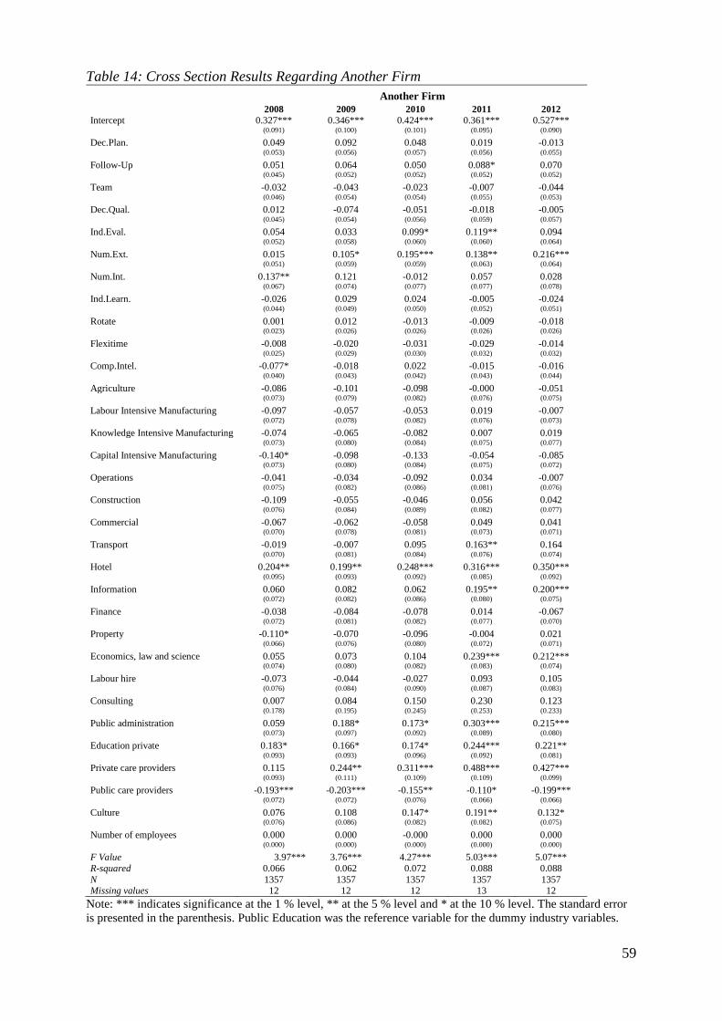
59
Table 14: Cross Section Results Regarding Another Firm
Another Firm
2008 2009 2010 2011 2012
Intercept 0.327*** 0.346*** 0.424*** 0.361*** 0.527***
(0.091) (0.100) (0.101) (0.095) (0.090)
Dec.Plan. 0.049 0.092 0.048 0.019 -0.013
(0.053) (0.056) (0.057) (0.056) (0.055)
Follow-Up 0.051 0.064 0.050 0.088* 0.070 (0.045) (0.052) (0.052) (0.052) (0.052)
Team -0.032 -0.043 -0.023 -0.007 -0.044
(0.046) (0.054) (0.054) (0.055) (0.053)
Dec.Qual. 0.012 -0.074 -0.051 -0.018 -0.005
(0.045) (0.054) (0.056) (0.059) (0.057)
Ind.Eval. 0.054 0.033 0.099* 0.119** 0.094
(0.052) (0.058) (0.060) (0.060) (0.064)
Num.Ext. 0.015 0.105* 0.195*** 0.138** 0.216*** (0.051) (0.059) (0.059) (0.063) (0.064)
Num.Int. 0.137** 0.121 -0.012 0.057 0.028
(0.067) (0.074) (0.077) (0.077) (0.078)
Ind.Learn. -0.026 0.029 0.024 -0.005 -0.024
(0.044) (0.049) (0.050) (0.052) (0.051)
Rotate 0.001 0.012 -0.013 -0.009 -0.018 (0.023) (0.026) (0.026) (0.026) (0.026)
Flexitime -0.008 -0.020 -0.031 -0.029 -0.014
(0.025) (0.029) (0.030) (0.032) (0.032)
Comp.Intel. -0.077* -0.018 0.022 -0.015 -0.016
(0.040) (0.043) (0.042) (0.043) (0.044)
Agriculture -0.086 -0.101 -0.098 -0.000 -0.051 (0.073) (0.079) (0.082) (0.076) (0.075)
Labour Intensive Manufacturing -0.097 -0.057 -0.053 0.019 -0.007
(0.072) (0.078) (0.082) (0.076) (0.073)
Knowledge Intensive Manufacturing -0.074 -0.065 -0.082 0.007 0.019
(0.073) (0.080) (0.084) (0.075) (0.077)
Capital Intensive Manufacturing -0.140* -0.098 -0.133 -0.054 -0.085 (0.073) (0.080) (0.084) (0.075) (0.072)
Operations -0.041 -0.034 -0.092 0.034 -0.007
(0.075) (0.082) (0.086) (0.081) (0.076)
Construction -0.109 -0.055 -0.046 0.056 0.042
(0.076) (0.084) (0.089) (0.082) (0.077)
Commercial -0.067 -0.062 -0.058 0.049 0.041 (0.070) (0.078) (0.081) (0.073) (0.071)
Transport -0.019 -0.007 0.095 0.163** 0.164
(0.070) (0.081) (0.084) (0.076) (0.074)
Hotel 0.204** 0.199** 0.248*** 0.316*** 0.350***
(0.095) (0.093) (0.092) (0.085) (0.092)
Information 0.060 0.082 0.062 0.195** 0.200*** (0.072) (0.082) (0.086) (0.080) (0.075)
Finance -0.038 -0.084 -0.078 0.014 -0.067
(0.072) (0.081) (0.082) (0.077) (0.070)
Property -0.110* -0.070 -0.096 -0.004 0.021
(0.066) (0.076) (0.080) (0.072) (0.071)
Economics, law and science 0.055 0.073 0.104 0.239*** 0.212*** (0.074) (0.080) (0.082) (0.083) (0.074)
Labour hire -0.073 -0.044 -0.027 0.093 0.105
(0.076) (0.084) (0.090) (0.087) (0.083)
Consulting 0.007 0.084 0.150 0.230 0.123
(0.178) (0.195) (0.245) (0.253) (0.233)
Public administration 0.059 0.188* 0.173* 0.303*** 0.215*** (0.073) (0.097) (0.092) (0.089) (0.080)
Education private 0.183* 0.166* 0.174* 0.244*** 0.221**
(0.093) (0.093) (0.096) (0.092) (0.081)
Private care providers 0.115 0.244** 0.311*** 0.488*** 0.427***
(0.093) (0.111) (0.109) (0.109) (0.099)
Public care providers -0.193*** -0.203*** -0.155** -0.110* -0.199***
(0.072) (0.072) (0.076) (0.066) (0.066)
Culture 0.076 0.108 0.147* 0.191** 0.132* (0.076) (0.086) (0.082) (0.082) (0.075)
Number of employees 0.000 0.000 -0.000 0.000 0.000
(0.000) (0.000) (0.000) (0.000) (0.000)
F Value 3.97*** 3.76*** 4.27*** 5.03*** 5.07***
R-squared 0.066 0.062 0.072 0.088 0.088
N 1357 1357 1357 1357 1357 Missing values 12 12 12 13 12
Note: *** indicates significance at the 1 % level, ** at the 5 % level and * at the 10 % level. The standard error
is presented in the parenthesis. Public Education was the reference variable for the dummy industry variables.

60
Table 15: Cross Section Results Regarding Negative Labour Market Status
Negative Labour Market Status
2008 2009 2010 2011 2012
Intercept 0.708*** 0.830*** 0.665*** 0.833*** 0.650***
(0.110) (0.109) (0.119) (0.120) (0.134)
Dec.Plan. 0.018 0.010 0.067 0.189** 0.186 (0.063) (0.070) (0.085) (0.092) (0.127)
Follow-Up -0.156** -0.072 -0.050 -0.103 -0.234
(0.075) (0.078) (0.090) (0.088) (0.165)
Team 0.054 0.045 0.077 -0.004 0.057
(0.068) (0.072) (0.090) (0.080) (0.101)
Dec.Qual. 0.066 0.009 0.084 -0.011 0.074 (0.071) (0.079) (0.091) (0.084) (0.183)
Ind.Eval. -0.067 0.012 -0.039 -0.091 0.050
(0.088) (0.090) (0.119) (0.124) (0.134)
Num.Ext. -0.121 -0.151 -0.392*** -0.261*** -0.434***
(0.108) (0.099) (0.086) (0.082) (0.140)
Num.Int. 0.225** 0.228** 0.359*** 0.255** 0.489*** (0.101) (0.104) (0.121) (0.115) (0.122)
Ind.Learn. -0.001 -0.064 0.051 0.026 -0.039
(0.072) (0.072) (0.088) (0.078) (0.083)
Rotate 0.027 0.019 0.054 0.081** -0.023
(0.033) (0.034) (0.040) (0.037) (0.049)
Flexitime -0.031 -0.090* -0.077 -0.062 -0.009 (0.050) (0.047) (0.053) (0.048) (0.067)
Comp.Intel. -0.027 -0.068 -0.022 -0.001 0.032
(0.058) (0.060) (0.070) (0.065) (0.096)
Agriculture -0.225** -0.227** -0.145 -0.131 0.038
(0.111) (0.115) (0.139) (0.149) (0.154)
Labour Intensive Manufacturing -0.129 -0.095 -0.053 -0.219** -0.036 (0.084) (0.081) (0.101) (0.093) (0.090)
Knowledge Intensive Manufacturing -0.241*** -0.179** -0.124 -0.197 -0.044
(0.079) (0.079) (0.110) (0.130) (0.116)
Capital Intensive Manufacturing -0.054 -0.079 0.066 -0.109 0.153
(0.091) (0.094) (0.108) (0.103) (0.104)
Operations -0.128 -0.231*** -0.156* -0.237** -0.071 (0.081) (0.077) (0.093) (0.095) (0.105)
Construction -0.263*** -0.239*** -0.216** -0.302*** -0.058
(0.079) (0.087) (0.096) (0.093) (0.101)
Commercial -0.196*** -0.223*** -0.156 -0.326*** -0.043
(0.074) (0.076) (0.095) (0.085) (0.088)
Transport -0.199*** -0.218*** -0.120 -0.136 -0.027
(0.075) (0.080) (0.104) (0.098) (0.098)
Hotel -0.075 -0.206** -0.072 -0.071 0.023 (0.076) (0.090) (0.099) (0.115) (0.110)
Information -0.205*** -0.133 -0.187* -0.196* 0.054
(0.080) (0.094) (0.104) (0.104) (0.109)
Finance -0.235*** -0.241*** -0.171* -0.302*** -0.127
(0.070) (0.079) (0.100) (0.090) (0.092)
Property -0.212*** -0.322*** -0.266*** -0.285*** -0.180* (0.067) (0.068) (0.095) (0.098) (0.099)
Economics, law and science -0.172 -0.197** -0.321*** -0.331*** 0.196
(0.109) (0.099) (0.086) (0.084) (0.391)
Labour hire 0.047 0.011 0.175 -0.002 0.106
(0.129) (0.126) (0.139) (0.124) (0.108)
Consulting -0.136 -0.093 -0.014 -0.213 -0.023 (0.202) (0.209) (0.214) (0.187) (0.206)
Public administration -0.031 0.029 0.076 -0.167* -0.033
(0.081) (0.094) (0.118) (0.096) (0.102)
Education private -0.003 -0.022 -0.085 -0.215** -0.045
(0.078) (0.088) (0.086) (0.090) (0.089)
Private care providers -0.059 -0.018 -0.192* -0.137 -0.084 (0.096) (0.101) (0.109) (0.109) (0.107)
Public care providers 0.008 -0.016 -0.075 -0.104 0.008
(0.072) (0.079) (0.095) (0.080) (0.085)
Culture 0.282** 0.146 0.334** 0.280** 0.301**
(0.132) (0.126) (0.164) (0.138) (0.141)
Number of employees 0.000** 0.000 0.000 -0.000 0.000 (0.000) (0.000) (0.000) (0.000) (0.000)
F Value 3.62*** 3.10*** 3.38*** 3.26*** 1.53**
Adjusted R-squared 0.059 0.048 0.054 0.051 0.013 N 1357 1357 1357 1357 1357
Missing values 12 12 12 13 13
Note: *** indicates significance at the 1 % level, ** at the 5 % level and * at the 10 % level. The standard error
is presented in the parenthesis. Public Education was the reference variable for the dummy industry variables.

61
Table 16: Cross Section Results Regarding Unemployed
Unemployed
2008 2009 2010 2011 2012
Intercept -0.244 1.198*** 0.702** 0.793* 0.473
(0.584) (0.425) (0.273) (0.474) (0.464)
Dec.Plan. 0.901*** 0.750 0.256 0.865** 0.864**
(0.345) (0.572) (0.223) (0.383) (0.338)
Follow-Up -0.656 -0.530 -0.004 0.092 -0.320 (0.424) (0.696) (0.241) (0.338) (0.300)
Team -0.003 -0.341 -0.015 0.319 0.262
(0.408) (0.441) (0.232) (0.296) (0.315)
Dec.Qual. 0.430 -1.201* -0.377 -1.145*** -0.274
(0.644) (0.694) (0.266) (0.390) (0.338)
Ind.Eval. 0.342 0.768 0.208 0.371 0.018
(0.315) (0.494) (0.261) (0.484) (0.361)
Num.Ext. 0.039 -0.283 -0.237 -0.229 -0.586** (0.481) (0.486) (0.231) (0.300) (0.284)
Num.Int. 0.093 -0.762 0.133 -0.818 0.695
(0.630) (0.571) (0.296) (0.529) (0.509)
Ind.Learn. 0.645 0.462 -0.269 0.101 0.137
(0.443) (0.659) (0.237) (0.350) (0.266)
Rotate 0.164 -0.091 -0.002 0.147 -0.109 (0.196) (0.283) (0.105) (0.167) (0.134)
Flexitime 0.204 0.048 -0.051 -0.555*** -0.177
(0.215) (0.236) (0.112) (0.164) (0.128)
Comp.Intel. -0.126 -0.028 0.013 -0.112 -0.056
(0.283) (0.183) (0.161) (0.238) (0.197)
Agriculture -0.351 -0.574* -0.240 -0.171 -0.058 (0.319) (0.296) (0.238) (0.462) (0.328)
Labour Intensive Manufacturing 0.068 -0.242 0.016 -0.195 0.129
(0.370) (0.333) (0.227) (0.430) (0.327)
Knowledge Intensive Manufacturing -0.259 0.963 0.239 0.070 0.405
(0.349) (1.390) (0.289) (0.601) (0.434)
Capital Intensive Manufacturing -0.029 -0.027 0.408 0.188 0.626* (0.341) (0.376) (0.259) (0.509) (0.373)
Operations -0.405 -0.837*** -0.343* -0.384 -0.296
(0.329) (0.273) (0.207) (0.419) (0.281)
Construction -0.202 -0.764** -0.318 -0.713 -0.243
(0.356) (0.319) (0.222) (0.434) (0.321)
Commercial -0.045 -0.421 0.301 -0.260 0.457 (0.394) (0.324) (0.290) (0.462) (0.402)
Transport -0.065 -0.707** -0.074 0.156 0.097
(0.357) (0.299) (0.236) (0.604) (0.314)
Hotel 0.033 -0.453 0.040 -0.428 0.057
(0.342) (0.356) (0.247) (0.417) (0.383)
Information -0.568* -0.427 0.385 0.493 0.393 (0.328) (0.577) (0.347) (0.622) (0.386)
Finance -0.371 -1.060*** -0.281 -0.310 -0.157
(0.360) (0.364) (0.204) (0.413) (0.328)
Property -0.155 -0.773*** -0.305 -0.525 -0.392
(0.354) (0.293) (0.192) (0.375) (0.264)
Economics, law and science -0.376 -0.810** 0.374 -0.185 -0.013 (0.338) (0.333) (0.398) (0.434) (0.407)
Labour hire 1.297* 0.348 0.282 0.367 0.274
(0.760) (0.406) (0.267) (0.533) (0.351)
Consulting 1.292 0.034 0.291 -0.194 -0.058
(0.793) (0.528) (0.449) (0.466) (0.540)
Public administration 1.977* 0.145 0.705 1.025 1.024 (1.071) (0.704) (0.469) (0.789) (0.782)
Education private 0.272 -0.427 -0.238 -0.374 -0.055
(0.394) (0.295) (0.235) (0.420) (0.312)
Private care providers 0.764 0.669 0.354 -0.207 -0.118
(0.598) (0.611) (0.399) (0.407) (0.312)
Public care providers -0.269 -0.504** -0.362 -0.169 -0.651*
(0.279) (0.235) (0.254) (0.419) (0.358)
Culture 1.699* 0.072 0.705* 0.262 1.101** (0.986) (0.374) (0.390) (0.487) (0.536)
Number of employees 0.000 -0.000 0.000 -0.000 0.000
(0.000) (0.000) (0.000) (0.000) (0.000)
F Value 2.72*** 1.27 1.88*** 1.50** 1.99***
Adjusted R-squared 0.040 0.006 0.021 0.012 0.023
N 1357 1357 1357 1357 1357 Missing values 18 31 19 17 19
Note: *** indicates significance at the 1 % level, ** at the 5 % level and * at the 10 % level. The standard error
is presented in the parenthesis. Public Education was the reference variable for the dummy industry variables.

62
Table 17: Cross Section Results Regarding Sick Leave
Sick Leave
2008 2009 2010 2011 2012
Intercept 1.099*** 1.316*** 0.296 1.258*** 0.859***
(0.265) (0.293) (0.251) (0.310) (0.279)
Dec.Plan. -0.054 -0.302 -0.058 0.088 -0.072
(0.146) (0.208) (0.192) (0.233) (0.219)
Follow-Up -0.018 0.023 0.070 -0.277 -0.297 (0.139) (0.214) (0.182) (0.214) (0.255)
Team 0.097 0.017 0.013 0.104 0.102
(0.169) (0.209) (0.194) (0.210) (0.181)
Dec.Qual. -0.243 -0.158 -0.018 -0.348 -0.063
(0.171) (0.242) (0.198) (0.245) (0.298)
Ind.Eval. -0.352 -0.246 0.286 -0.380 -0.134
(0.290) (0.261) (0.203) (0.263) (0.218)
Num.Ext. -0.359*** -0.321* -0.502*** -0.379* -0.480** (0.136) (0.184) (0.193) (0.213) (0.231)
Num.Int. 0.075 0.257 0.577** 0.460* 0.759***
(0.221) (0.269) (0.240) (0.256) (0.237)
Ind.Learn. -0.086 0.012 0.237 0.213 -0.019
(0.160) (0.179) (0.181) (0.184) (0.152)
Rotate 0.039 -0.091 0.035 0.072 -0.021 (0.074) (0.086) (0.086) (0.101) (0.088)
Flexitime -0.181** -0.284** -0.076 0.015 0.033
(0.086) (0.113) (0.115) (0.122) (0.116)
Comp.Intel. 0.051 0.028 -0.009 -0.020 0.135
(0.123) (0.150) (0.143) (0.165) (0.167)
Agriculture -0.318* -0.426 0.308 0.025 -0.163 (0.190) (0.288) (0.321) (0.354) (0.276)
Labour Intensive Manufacturing 0.029 0.184 0.291 -0.208 0.050
(0.193) (0.261) (0.235) (0.230) (0.205)
Knowledge Intensive Manufacturing -0.065 -0.032 -0.068 -0.431* -0.138
(0.198) (0.268) (0.231) (0.243) (0.205)
Capital Intensive Manufacturing 0.242 -0.184 0.166 -0.271 0.228 (0.221) (0.219) (0.206) (0.236) (0.221)
Operations 0.082 0.052 0.254 -0.168 -0.188
(0.186) (0.266) (0.238) (0.249) (0.185)
Construction -0.250 -0.165 0.287 -0.373 0.243
(0.175) (0.255) (0.267) (0.257) (0.246)
Commercial 0.009 -0.118 -0.214 -0.371 -0.120 (0.321) (0.244) (0.186) (0.226) (0.194)
Transport 0.009 -0.072 -0.122 0.131 -0.107
(0.185) (0.234) (0.193) (0.313) (0.193)
Hotel 0.132 -0.413* -0.053 -0.117 -0.020
(0.234) (0.217) (0.255) (0.302) (0.282)
Information -0.138 -0.305 -0.142 0.072 0.006 (0.227) (0.209) (0.253) (0.441) (0.299)
Finance -0.281 -0.460** -0.463** -0.641*** -0.273
(0.173) (0.190) (0.186) (0.223) (0.200)
Property -0.134 -0.211 -0.027 -0.270 0.181
(0.158) (0.204) (0.212) (0.223) (0.230)
Economics, law and science -0.384*** -0.419** -0.353* -0.637*** 0.189 (0.147 (0.208) (0.204) (0.221) (0.578)
Labour hire -0.213 -0.420** 0.113 -0.291 0.277
(0.181) (0.206) (0.232) (0.250) (0.250)
Consulting -0.317 -0.241 0.249 -0.570* -0.037
(0.206) (0.300) (0.351) (0.302) (0.295)
Public administration 0.182 0.699* 0.694* -0.307 -0.116 (0.187) (0.393) (0.357) (0.252) (0.206)
Education private -0.177 -0.117 -0.252 -0.466** -0.097
(0.156) (0.221) (0.177) (0.204) (0.209)
Private care providers -0.078 -0.461** -0.292 -0.075 -0.268
(0.251) (0.190) (0.205) (0.307) (0.179)
Public care providers 0.187 0.368 0.069 0.294 0.452**
(0.175) (0.249) (0.206) (0.220) (0.209)
Culture -0.024 -0.047 0.063 -0.109 -0.155 (0.197) (0.240) (0.251) (0.291) (0.247)
Number of employees 0.000 -0.000 0.000 -0.000 0.000*
(0.000) (0.000) (0.000) (0.000) (0.000)
F Value 1.63** 2.22*** 1.73*** 1.63** 1.36*
Adjusted R-squared 0.015 0.028 0.017 0.015 0.008
N 1357 1357 1357 1357 1357 Missing values 12 12 12 13 13
Note: *** indicates significance at the 1 % level, ** at the 5 % level and * at the 10 % level. The standard error
is presented in the parenthesis. Public Education was the reference variable for the dummy industry variables.

63
Table 18: Cross Section Results Regarding Disability Pensioner Disability Pensioner 2008 2009 2010 2011 2012
Intercept 0.577 0.531 0.659** 0.810* 0.539* (0.434) (0.367) (0.284) (0.415) (0.323)
Dec.Plan. 0.089 0.250 0.014 0.125 0.350 (0.293) (0.245) (0.191) (0.356) (0.328)
Follow-Up -0.352 -0.277 -0.301 -0.627 -0.529 (0.374) (0.310) (0.244) (0.383) (0.381)
Team 0.719* 0.681** 0.271 0.639 0.185 (0.409) (0.341) (0.229) (0.437) (0.273)
Dec.Qual. 0.211 0.302 0.477* 0.294 0.465* (0.358) (0.296) (0.248) (0.339) (0.265)
Ind.Eval. -0.248 -0.254 -0.230 -0.275 0.271 (0.352) (0.299) (0.241) (0.409) (0.311)
Num.Ext. -0.738 -0.539 -0.795*** -0.314 -0.730** (0.491) (0.404) (0.287) (0.608) (0.286)
Num.Int. 0.513 0.556* 0.500 0.354 0.366 (0.404) (0.310) (0.306) (0.423) (0.366)
Ind.Learn. -0.062 -0.065 0.150 0.262 0.262 (0.352) (0.286) (0.262) (0.289) (0.288)
Rotate 0.272* 0.377*** 0.271*** 0.493*** 0.268** (0.143) (0.141) (0.096) (0.162) (0.127)
Flexitime -0.191 -0.050 0.007 -0.056 -0.268 (0.252) (0.200) (0.147) (0.191) (0.171)
Comp.Intel. 0.252 -0.195 0.104 -0.148 0.033 (0.275) (0.363) (0.201) (0.377) (0.283)
Agriculture -0.110 -0.133 -0.242 0.141 0.290 (0.345) (0.336) (0.349) (0.820) (0.874)
Labour Intensive Manufacturing 0.113 -0.064 -0.075 -0.399 -0.184 (0.349) (0.261) (0.262) (0.272) (0.222)
Knowledge Intensive Manufacturing 0.042 -0.206 -0.233 -0.291 -0.354 (0.466) (0.299) (0.303) (0.391) (0.232)
Capital Intensive Manufacturing 0.367 0.140 0.033 -0.143 0.013 (0.388) (0.258) (0.252) (0.321) (0.288)
Operations 0.970 0.756 0.333 0.353 0.268 (0.961) (0.792) (0.432) (0.539) (0.469)
Construction 0.006 0.055 -0.074 -0.200 0.087 (0.326) (0.289) (0.302) (0.382) (0.363)
Commercial -0.126 -0.223 -0.325* -0.355 -0.357* (0.219) (0.201) (0.187) (0.238) (0.213)
Transport -0.211 -0.186 -0.306 -0.192 -0.093 (0.224) (0.198) (0.189) (0.251) (0.236)
Hotel -0.475* -0.498** -0.628*** -0.643** -0.632** (0.266) (0.232) (0.230) (0.271) (0.269)
Information -0.003 0.850 -0.074 0.663 0.075 (0.303) (0.987) (0.239) (0.911) (0.332)
Finance 0.884 0.501 0.160 0.801 -0.099 (0.597) (0.471) (0.356) (0.765) (0.303)
Property -0.368** -0.326** -0.453*** -0.426** -0.452** (0.161) (0.150) (0.157) (0.194) (0.201)
Economics, law and science -0.180 -0.392* -0.579*** -0.591** -0.420* (0.292) (0.212) (0.171) (0.239) (0.220)
Labour hire -0.189 -0.188 -0.222 -0.171 -0.236 (0.263) (0.253) (0.252) (0.315) (0.298)
Consulting -0.208 -0.272 -0.318 -0.340 -0.352 (0.527) (0.535) (0.546) (0.603) (0.595)
Public administration -0.123 -0.225 -0.372* -0.371 -0.288 (0.263) (0.234) (0.197) (0.235) (0.228)
Education private -0.208 -0.197 -0.256 -0.296 -0.326 (0.186) (0.164) (0.174) (0.196) (0.199)
Private care providers -0.309 -0.263 -0.305 -0.316 -0.508** (0.207) (0.203) (0.213) (0.237) (0.219)
Public care providers 0.048 0.037 0.041 0.005 -0.022 (0.201) (0.203) (0.243) (0.274) (0.271)
Culture 1.080* 0.885* 0.911* 1.141** 0.905* (0.554) (0.481) (0.480) (0.517) (0.497)
Number of employees 0.000 0.000 0.000 0.000 0.000 (0.000) (0.000) (0.000) (0.000) (0.000)
F Value 1.24 1.34* 2.02*** 1.35* 1.38* Adjusted R-squared 0.006 0.008 0.024 0.009 0.009
N 1313 1315 1312 1307 1304
Missing values 44 42 45 50 53
Note: *** indicates significance at the 1 % level, ** at the 5 % level and * at the 10 % level. The standard error
is presented in the parenthesis. Public Education was the reference variable for the dummy industry variables.

64
Table 19: Cross Section Results Regarding Other, Low Income Other, Low Income
2008 2009 2010 2011 2012 Intercept 0.408*** 0.555 0.564*** 0.661*** 0.319** (0.109) (0.555) (0.167) (0.146) (0.149)
Dec.Plan. 0.002 0.155 0.113 0.145 0.303*** (0.063) (0.088) (0.121) (0.090) (0.102)
Follow-Up -0.039 0.001 0.154 0.109 0.138 (0.078) (0.089) (0.096) (0.087) (0.101)
Team -0.022 -0.069 -0.041 -0.119 0.009 (0.082) (0.099) (0.123) (0.095) (0.113)
Dec.Qual. -0.011 0.045 0.156 0.049 -0.108 (0.072) (0.100) (0.131) (0.113) (0.116)
Ind.Eval. -0.043 0.021 -0.213 -0.106 -0.072 (0.090) (0.110) (0.166) (0.119) (0.132)
Num.Ext. 0.082 -0.011 -0.187* -0.041 -0.134 (0.106) (0.128) (0.109) (0.093) (0.114)
Num.Int. 0.255** 0.163 0.207 0.225* 0.359** (0.102) (0.115) (0.165) (0.132) (0.147)
Ind.Learn. -0.029 -0.116 0.086 -0.083 -0.092 (0.066) (0.085) (0.095) (0.089) (0.106)
Rotate -0.021 -0.046 -0.031 0.013 -0.060 (0.035) (0.043) (0.056 (0.046) (0.053)
Flexitime 0.007 -0.041 -0.047 -0.040 0.021 (0.056) (0.064) (0.075) (0.055) (0.066)
Comp.Intel. -0.097 -0.094 -0.089 0.010 -0.069 (0.064) (0.074) (0.095) (0.078) (0.089)
Agriculture -0.050 -0.006 -0.033 -0.169 0.296* (0.092) (0.142) (0.212) (0.132) (0.168)
Labour Intensive Manufacturing -0.074 -0.046 -0.203 -0.180 0.081 (0.076) (0.104) (0.129) (0.132) (0.126)
Knowledge Intensive Manufacturing -0.158 -0.141 -0.328*** -0.236** -0.013 (0.072) (0.112) (0.119) (0.120) (0.107)
Capital Intensive Manufacturing -0.115 -0.113 -0.172 -0.122 0.136 (0.072) (0.111) (0.137) (0.137) (0.118)
Operations -0.140* -0.181 -0.264** -0.243 0.189 (0.075) (0.114) (0.131) (0.150) (0.179)
Construction -0.097 -0.045 -0.244* -0.180 0.127 (0.085) (0.112) (0.148) (0.130) (0.126)
Commercial -0.084 -0.148 -0.213* -0.257** 0.036 (0.073) (0.099) (0.118) (0.115) (0.110)
Transport -0.121* -0.048 0.116 -0.114 0.171 (0.073) (0.125) (0.253) (0.148) (0.149)
Hotel 0.175* 0.120 0.239 0.136 0.334** (0.093) (0.117) (0.167) (0.160) (0.141)
Information 0.005 0.036 -0.228* -0.164 0.201 (0.084) (0.121) (0.130) (0.126) (0.153)
Finance -0.140** -0.087 -0.043 -0.219* 0.067 (0.066) (0.106) (0.161) (0.117) (0.122)
Property -0.017 -0.177 -0.280* -0.147 -0.025 (0.085) (0.107) (0.147) (0.147) (0.127)
Economics, law and science 0.123 0.123 -0.316*** -0.100 0.134 (0.129) (0.157) (0.116) (0.136) (0.151)
Labour hire 0.215 0.106 0.374 0.111 0.254 (0.166) (0.129) (0.250) (0.171) (0.172)
Consulting -0.141 -0.109 -0.234 -0.127 0.033 (0.145) (0.188) (0.163) (0.201) (0.235)
Public administration -0.058 -0.025 -0.175 -0.103 0.173 (0.074) (0.120) (0.135) (0.132) (0.148)
Education private 0.192** 0.238 0.138 -0.105 0.143 (0.086) (0.118) (0.150) (0.124) (0.109)
Private care providers 0.149 0.204 -0.184 -0.129 0.262 (0.173) (0.159) (0.147) (0.132) (0.180)
Public care providers -0.072 -0.110 -0.203 -0.286*** -0.089 (0.064) (0.093) (0.123) (0.105) (0.103)
Culture 0.051 -0.030 -0.050 0.137 0.253* (0.100) (0.112) (0.147) (0.137) (0.138)
Number of employees 0.000* 0.000 0.000 -5.871E-9 0.000 (0.000) (0.000) (0.000) (0.000) (0.000)
F value 2.61*** 2.02*** 2.47*** 1.77*** 1.52**
Adjusted R-squared 0.037 0.024 0.034 0.018 0.012 N 1345 1345 1344 1344 1343
Missing values 12 12 13 13 14
Note: *** indicates significance at the 1 % level, ** at the 5 % level and * at the 10 % level. The standard error
is presented in the parenthesis. Public Education was the reference variable for the dummy industry variables.

65
Table 20: Cross Section Results Regarding Employed after the Age of 65 Employed after the Age of 65 2008 2009 2010 2011 2012
Intercept 0.163*** 0.190*** 0.248*** 0.294*** 0.303*** (0.024) (0.029) (0.036) (0.039) (0.036)
Dec.Plan. -0.040*** -0.047*** -0.060*** -0.050*** -0.070*** (0.013) (0.015) (0.021) (0.018) (0.025)
Follow-Up -0.084*** -0.062*** -0.067** -0.075*** -0.063** (0.020) (0.021) (0.026) (0.025) (0.029)
Team 0.017 0.046*** 0.040* 0.040** 0.019 (0.014) (0.017) (0.022) (0.018) (0.024)
Dec.Qual. 0.030** 0.029 0.002 0.057** 0.042* (0.015) (0.018) (0.021) (0.023) (0.024)
Ind.Eval. -0.031 -0.064*** -0.105*** -0.065*** -0.114*** (0.020) (0.023) (0.030) (0.025) (0.035)
Num.Ext. -0.079*** -0.080*** -0.091*** -0.102*** -0.088*** (0.012) (0.017) (0.023) (0.020) (0.026)
Num.Int. -0.062** -0.067** -0.064** -0.060** -0.027 (0.025) (0.028) (0.033) (0.030) (0.035)
Ind.Learn. 0.016 0.004 0.002 -0.020 -0.026 (0.015) (0.018) (0.021) (0.021) (0.025)
Rotate -0.009 -0.011 -0.003 -0.008 -0.027** (0.006) (0.007) (0.010) (0.009) (0.011)
Flexitime 0.012 -0.005 0.001 0.001 0.026* (0.009) (0.011) (0.014) (0.012) (0.015)
Comp.Intel. 0.018 0.022 0.034* 0.013 0.007 (0.013) (0.014) (0.018) (0.014) (0.019)
Agriculture 0.038 0.037 0.051 0.012 0.052 (0.030) (0.033) (0.032) (0.029) (0.036)
Labour Intensive Manufacturing -0.014 -0.011 -0.009 -0.063** -0.005 (0.015) (0.020) (0.026) (0.030) (0.030)
Knowledge Intensive Manufacturing 0.007 -0.009 -0.009 -0.052* 0.001 (0.017) (0.019) (0.023) (0.029) (0.030)
Capital Intensive Manufacturing -0.014 -0.022 -0.045** -0.102*** -0.065*** (0.016) (0.021) (0.022) (0.027) (0.021)
Operations -0.009 -0.004 -0.015 -0.030 0.027 (0.015) (0.019) (0.022) (0.031) (0.025)
Construction -0.037** -0.028 -0.015 -0.071*** -0.005 (0.015) (0.019) (0.023) (0.027) (0.029)
Commercial -0.024* -0.034** -0.037** -0.092*** -0.045** (0.013) (0.017) (0.019) (0.025) (0.022)
Transport 0.004 0.007 0.023 -0.027 0.028 (0.014) (0.020) (0.027) (0.029) (0.028)
Hotel -0.007 -0.026 -0.052*** -0.096*** -0.048** (0.014) (0.017) (0.017) (0.025) (0.023)
Information -0.000 0.007 0.001 -0.058* -0.034 (0.022) (0.026) (0.037) (0.034) (0.021)
Finance -0.018 -0.000 -0.004 -0.044 -0.007 (0.016) (0.021) (0.026) (0.027) (0.025)
Property -0.016 -0.015 0.013 -0.030 0.039 (0.015) (0.018) (0.021) (0.028) (0.028)
Economics, law and science 0.006 0.037 0.065* 0.006 0.084** (0.021) (0.028) (0.035) (0.034) (0.042)
Labour hire -0.025* -0.040** -0.052** -0.088*** -0.075*** (0.015) (0.016) (0.022) (0.028) (0.023)
Consulting -0.055*** -0.068*** -0.093*** -0.117*** -0.068** (0.017) (0.017) (0.021) (0.032) (0.030)
Public administration 0.0016 0.018 0.028 0.002 0.039 (0.015) (0.019) (0.021) (0.027) (0.025)
Education private 0.019 0.015 0.012 -0.021 0.013 (0.017) (0.020) (0.023) (0.027) (0.024)
Private care providers 0.016 0.013 0.024 -0.034 0.033 (0.017) (0.019) (0.023) (0.027) (0.026)
Public care providers -0.006 -0.003 0.027 -0.025 0.025 (0.013) (0.014) (0.022) (0.027) (0.022)
Culture 0.000 -0.001 -0.023 -0.014 -0.027 (0.015) (0.017) (0.017) (0.030) (0.026)
Number of employees -0.000 -0.000 -0.000 -0.000 0.000 (0.000) (0.00) (0.000) (0.000) (0.000)
F Value 4.95*** 4.35*** 4.44*** 5.22*** 4.68***
Adjusted R-squared 0.141 0.109 0.104 0.119 0.101 N 769 875 952 1000 1049
Missing values 588 482 405 357 308
Note: *** indicates significance at the 1 % level, ** at the 5 % level and * at the 10 % level. The standard error
is presented in the parenthesis. Public Education was the reference variable for the dummy industry variables.

66
Table 21: Cross Section Results Regarding Early Pensioner Early Pensioner 2008 2009 2010 2011 2012
Intercept 0.588** 0.587** 1.062 1.533*** 1.474*** (0.287) (0.284) (0.659) (0.464) (0.440)
Dec.Plan. 0.386 0.145 0.265 -0.152 0.016 (0.249) (0.231) (0.414) (0.261) (0.247)
Follow-Up 0.353 0.524 -0.512 -0.190 -0.268 (0.294) (0.332) (0.690) (0.396) (0.369)
Team -0.092 -0.487 0.170 -0.163 -0.298 (0.348) (0.566) (0.705) (0.281) (0.252)
Dec.Qual. -0.109 0.122 -0.104 0.045 -0.108 (0.257) (0.370) (0.751) (0.356) (0.339)
Ind.Eval. -0.256 0.219 0.574 0.056 0.095 (0.367) (0.314) (0.813) (0.471) (0.391)
Num.Ext. -0.263 -0.413 -0.755 -0.192 -0.318 (0.287) (0.391) (0.461) (0.273) (0.244)
Num.Int. -0.383 -0.955 -0.401 -0.448 -0.516 (0.545) (0.682) (0.787) (0.602) (0.441)
Ind.Learn. 0.207 0.316 0.348 0.129 0.454* (0.266) (0.373) (0.456) (0.323) (0.251)
Rotate 0.038 0.328** 0.242 0.270* 0.273** (0.143) (0.142) (0.302) (0.154) (0.120)
Flexitime -0.259 -0.182 -0.308 -0.070 0.029 (0.181) (0.184) (0.357) (0.244) (0.204)
Comp.Intel. 0.102 -0.319 -0.615 -0.206 -0.338 (0.287) (0.287) (0.560) (0.376) (0.257)
Agriculture -0.078 -0.133 -0.338 -0.858*** -0.563** (0.190) (0.169) (0.335) (0.227) (0.238)
Labour Intensive Manufacturing 0.698*** 0.423** 0.928 0.081 0.210 (0.253) (0.210) (0.660) (0.437) (0.408)
Knowledge Intensive Manufacturing 0.494* 0.040 0.044 -0.302 -0.354 (0.261) (0.197) (0.327) (0.239) (-0.354)
Capital Intensive Manufacturing 0.642** 0.167 -0.043 -0.178 -0.109 (0.309) (0.250) (0.350) (0.265) (0.241)
Operations 0.392 0.068 -0.055 -0.163 -0.201 (0.272) (0.177) (0.274) (0.240) (0.237)
Construction 0.314 0.138 0.473 -0.360 -0.471** (0.295) (0.222) (0.651) (0.260) (0.239)
Commercial 0.561** 0.394 0.115 -0.258 -0.422** (0.280) (0.268) (0.256) (0.221) (0.196)
Transport 1.270* 1.135 1.326 0.991 0.537 (0.695) (0.791) (1.128) (1.093) (0.740)
Hotel 2.029* 3.668 2.434 0.394 0.268 (1.181) (2.593) (1.851) (0.798) (0.656)
Information 0.175 0.373 0.100 -0.253 0.269 (0.236) (0.257) (0.294) (0.249) (0.421)
Finance 0.649*** 0.650*** 0.839*** 0.389* 0.331 (0.210) (0.197) (0.258) (0.217) (0.244)
Property 0.231 0.409** 0.427* 0.232 -0.055 (0.164) (0.173) (0.243) (0.211) (0.184)
Economics, law and science 0.393* 0.529** 0.240 -0.140 -0.335* (0.213) (0.241) (0.271) (0.213) (0.194)
Labour hire 0.819 0.276 1.042 0.226 -0.229 (0.718) (0.262) (0.717) (0.566) (0.253)
Consulting 1.034 -0.024 18.819 -0.686*** -0.811*** (0.641) (0.281) (16.742) (0.231) (0.221)
Public administration 0.524*** 0.403** 0.331 -0.126 -0.122 (0.196) (0.174) (0.248) (0.187) (0.176)
Education private 0.703** 0.647* 0.683 0.178 -0.000 (0.294) (0.372) (0.488) (0.411) (0.183)
Private care providers 1.520** 1.059* 1.008 0.150 0.048 (0.768) (0.568) (0.693) (0.279) (0.205)
Public care providers 0.270 0.316* 0.368 -0.081 0.232 (0.173) (0.165) (0.239) (0.161) (0.194)
Culture 0.740** 0.601** 0.377 -0.196 0.143 (0.319) (0.299) (0.404) (0.330) (0.368)
Number of employees -0.000 -0.000 -0.000 -0.000 -0.000 (0.000) (0.000) (0.000) (0.000) (0.000)
F Value 1.46** 1.87*** 3.74*** 0.80 1.12
Adjusted R-squared 0.011 0.020 0.061 -0.005 0.003
N 1340 1344 1343 1344 1344 Missing values 17 13 14 13 13
Note: *** indicates significance at the 1 % level, ** at the 5 % level and * at the 10 % level. The standard error
is presented in the parenthesis. Public Education was the reference variable for the dummy industry variables.

67
Table 22: Cross Section Results Regarding Student Student 2008 2009 2010 2011 2012
Intercept -0.255* -2.557 0.070 -0.309 0.251 (0.133) (2.926) (0.662) (0.472) (0.244)
Dec.Plan. 0.220* -5.719 -1.238 -0.494 -0.238 (0.118) (5.743) (1.190) (0.624) (0.377)
Follow-Up 0.182* -6.937 0.769* -0.110 -0.238 (0.099) (7.070) (0.465) (0.256) (0.415)
Team -0.134 14.504 0.609 0.240 -0.049 (0.117) (13.800) (0.456) (0.297) (0.185)
Dec.Qual. -0.047 10.068 0.557 0.480 0.266 (0.113) (9.756) (0.397) (0.491) (0.312)
Ind.Eval. 0.263** 7.719 0.423 0.627 0.389 (0.127) (7.571) (0.328) (0.698) (0.478)
Num.Ext. -0.185 13.811 0.864 -1.172 -0.386 (0.127) (13.769) (1.279) (0.785) (0.299)
Num.Int. 0.549*** 15.150 -0.231 1.913 0.183 (0.128) (14.174) (1.200) (1.810) (0.374)
Ind.Learn. 0.019 -12.865 -0.476 -0.274 0.033 (0.124) (12.519) (0.367) (0.434) (0.309)
Rotate 0.008 -4.540 -0.111 -0.536 -0.026 (0.050) (4.446) (0.110) (0.562) (0.108)
Flexitime -0.170*** 3.693 0.377 0.020 -0.045 (0.065) (3.789) (0.413) (0.122) (0.173)
Comp.Intel. -0.120 -4.514 -0.337** -0.145 0.045 (0.082) (4.422) (0.171) (0.214) (0.224)
Agriculture 0.114 1.413 -0.239 0.413 -0.110 (0.078) (1.799) (0.473) (0.310) (0.195)
Labour Intensive Manufacturing 0.763*** 1.947 0.023 1.164** 0.657* (0.245) (1.862) (0.754) (0.541) (0.350)
Knowledge Intensive Manufacturing 0.312*** 0.902 2.360 1.412** 1.078* (0.093) (1.382) (1.485) (0.674) (0.563)
Capital Intensive Manufacturing 0.485* 1.988 -0.107 0.938* 0.378 (0.148) (1.980) (0.678) (0.507) (0.282)
Operations 0.133** 0.092 -0.569 0.627 0.025 (0.081) (1.279) (0.757) (0.466) (0.199)
Construction 0.292*** 2.346 -0.142 1.009* 0.159 (0.115) (2.387) (0.690) (0.602) (0.253)
Commercial 0.402** 1.172 0.154 4.004 0.658* (0.104) (1.376) (0.352) (3.499) (0.354)
Transport 0.420 3.733 0.103 0.731** 0.583 (0.185) (3.511) (0.365) (0.364) (0.476)
Hotel 0.308*** 0.931 0.254 0.662*** 0.413** (0.103) (1.446) (0.298) (0.202) (0.185)
Information 0.349** -1.675 -0.025 0.544 0.058 (0.160) (2.181) (0.714) (0.449) (0.241)
Finance 0.731*** 0.654 0.314 0.967* 0.086 (0.224) (1.338) (0.599) (0.508) (0.191)
Property 0.095 0.273 0.030 0.819 0.564 (0.068) (1.166) (0.402) (0.515) (0.406)
Economics, law and science 0.188** -3.288 -0.456 0.345 -0.066 (0.090) (3.544) (0.582) (0.272) (0.216)
Labour hire 0.522*** 0.763 0.053 0.654*** 0.337** (0.123) (1.452) (0.426) (0.223) (0.142)
Consulting 0.383 1.805 0.335 0.230 0.166 (0.237) (2.802) (0.324) (0.306) (0.244)
Public administration 0.158* -1.787 0.450 0.268 -0.032 (0.082) (2.400) (0.718) (0.264) (0.204)
Education private 0.198** -1.025 -0.087 0.235** 0.043 (0.077) (1.548) (0.228) (0.118) (0.114)
Private care providers 0.369*** -0.718 0.019 0.322** 0.108 (0.099) (1.531) (0.257) (0.158) (0.105)
Public care providers 0.195** -0.346 0.109 0.249** 0.154 (0.077) (1.106) (0.154) (0.112) (0.098)
Culture 0.646*** 36.672 0.522 0.316* 0.267* (0.152) (35.383) (0.447) (0.176) (0.160)
Number of employees 0.000 -0.000 -0.000 0.000 -0.000 (0.000) (0.000) (0.000) (0.000) (0.000)
F Value 3.60*** 1.30 0.99 0.88 1.07
Adjusted R-squared 0.064 0.008 -0.000 -0.003 0.002 N 1229 1206 1193 1209 1199
Missing values 128 151 164 148 158
Note: *** indicates significance at the 1 % level, ** at the 5 % level and * at the 10 % level. The standard error
is presented in the parenthesis. Public Education was the reference variable for the dummy industry variables.

68
Table 23: Cross Section Results Regarding Other, High Income Other, High Income 2008 2009 2010 2011 2012
Intercept 0.285 1.617** 1.332* 1.450 -0.276 (0.646) (0.688) (0.737) (1.430) (0.333)
Dec.Plan. 0.077 -0.131 -0.772 -0.348 0.010 (0.457) (0.436) (0.612) (0.380) (0.310)
Follow-Up -0.523 -0.082 0.019 0.556 0.237 (0.419) (0.293) (0.468) (0.437) (0.287)
Team 0.441 -0.428 -0.481 -1.258 0.484 (0.485) (0.490) (0.327) (0.815) (0.417)
Dec.Qual. -0.048 -0.071 0.384 -1.770 -0.333 (0.450) (0.391) (0.738) (1.565) (0.326)
Ind.Eval. 0.939 -0.083 0.205 -0.829 0.531 (0.643) (0.389) (0.354) (0.820) (0.377)
Num.Ext. -0.138 -0.319 -0.151 -0.815 0.262 (0.649) (0.481) (0.352) (1.022) (0.382)
Num.Int. 0.616 -0.420 -0.208 1.316 -0.164 (0.571) (0.574) (0.599) (1.152) (0.409)
Ind.Learn. -0.401 0.302 0.023 -0.925 0.334 (0.471) (0.314) (0.277) (1.246) (0.292)
Rotate 0.593*** 0.494** -0.084 -0.299 -0.108 (0.215) (0.236) (0.181) (0.557) (0.164)
Flexitime 0.169 0.491 -0.004 -0.820 0.125 (0.343) (0.312) (0.281) (0.655) (0.220)
Comp.Intel. -0.205 -0.125 0.030 1.425 -0.114 (0.395) (0.311) (0.321) (1.423) (0.185)
Agriculture 0.099 -1.457** -0.923*** -0.149 -0.019 (0.613) (0.684) (0.306) (0.204) (0.266)
Labour Intensive Manufacturing -0.477 -1.290* -0.589* 0.139 0.526 (0.410) (0.695) (0.321) (0.267) (0.441)
Knowledge Intensive Manufacturing -0.827** -0.773 0.058 1.360 -0.083 (0.401) (0.744) (0.488) (0.939) (0.262)
Capital Intensive Manufacturing -0.428 -1.153 -0.123 0.624 0.112 (0.455) (0.748) (0.735) (0.498) (0.280)
Operations -0.346 -1.327** -0.699** 0.336 -0.449** (0.413) (0.676) (-0.699) (0.301) (0.206)
Construction -0.166 -1.278* -0.785** 0.130 0.634 (0.511) (0.666) (0.387) (0.202) (0.622)
Commercial 0.013 -1.243* -0.536* 0.269 0.531 (0.829) (0.690) (0.301) (0.236) (0.476)
Transport 0.008 0.576 0.032 -0.453 0.108 (0.757) (1.309) (0.439) (0.378) (0.251)
Hotel 0.080 -0.962 -0.294 -0.489 0.830 (0.5789) (0.724) (0.325) (0.304) (0.530)
Information 1.282 -0.755 0.011 0.596 -0.505** (1.446) (0.859) (0.402) (0.535) (0.244)
Finance -0.478 -1.525** -0.203 1.645 0.097 (0.388) (0.659) (0.427) (1.333) (0.498)
Property -0.116 -1.219* -0.107 6.000 -0.399** (0.406) (0.676) (0.496) (5.881) (0.189)
Economics, law and science -0.311 -0.763 -0.289 0.671 -0.215 (0.519) (0.727) (0.310) (0.481) (0.317)
Labour hire -0.063 -0.887 -0.310 -0.457 0.703 (0.535) (0.689) (0.363) (0.394) (0.463)
Consulting -0.206 -0.586 0.263 1.636 0.035 (0.551) (0.766) (0.665) (1.899) (0.289)
Public administration -0.897*** -1.016 1.149 0.699 0.368 (0.343) (0.665) (1.150) (0.467) (0.433)
Education private 0.098 -0.571 0.230 -0.121 0.095 (0.520) (0.696) (0.579) (0.177) (0.280)
Private care providers -0.058 -1.138* -0.175 -0.262 1.254 (0.551) (0.670) (0.344) (0.239) (1.097)
Public care providers -0.101 -0.844 0.382 -0.092 0.160 (0.484) (0.632) (0.526) (0.126) (0.384)
Culture 0.279 -0.413 0.144 -0.291 0.701 (0.796) (0.825) (0.508) (0.334) (0.492)
Number of employees 0.000 -0.000 -0.000* 0.000 -0.000 (0.000) (0.000) (0.000) (0.000) (0.000)
F value 0.99 1.11 0.75 0.70 1.52**
Adjusted R-squared -0.000 0.003 -0.006 -0.007 0.012
N 1344 1345 1345 1307 1344 Missing values 13 12 12 50 13
Note: *** indicates significance at the 1 % level, ** at the 5 % level and * at the 10 % level. The standard error
is presented in the parenthesis. Public Education was the reference variable for the dummy industry variables.

69
Appendix C – Panel Data Results with all Parameters
Table 24: Panel Data Results Regarding Employed to Sick Leave
Employed Same Firm Another Firm Negative Unemployed Sick Leave
Intercept 1.090*** 1.371*** 0.406*** 0.733*** 0.649** 0.964***
(0.022) (0.054) (0.086) (0.090) (0.297) (0.165)
Dec.Plan. -0.025* -0.076** 0.040 0.094 0.686*** -0.079 (0.013) (0.034) (0.049) (0.064) (0.228) (0.125)
Follow-Up 0.021 -0.054 0.065 -0.123* -0.302 -0.100
(0.016) (0.040) (0.046) (0.072) (0.257) (0.120)
Team -0.002 0.020 -0.030 0.045 0.047 0.066
(0.014) (0.034) (0.045) (0.060) (0.184) (0.121)
Dec.Qual. -0.003 0.036 -0.029 0.043 -0.525* -0.167 (0.014) (0.038) (0.048) (0.068) (0.301) (0.136)
Ind.Eval. -0.010 -0.057 0.082 -0.027 0.346 -0.165
(0.018) (0.042) (0.050) (0.083) (0.256) (0.149)
Num.Ext. 0.027** -0.045 0.136*** -0.272*** -0.241 -0.408***
(0.014) (0.041) (0.052) (0.069) (0.210) (0.114)
Num.Int. -0.042** -0.064 0.065 0.311*** -0.194 0.425*** (0.021) (0.054) (0.067) (0.088) (0.357) (0.146)
Ind.Learn. -0.0047 -0.028 -0.000 -0.004 0.186 0.072
(0.014) (0.033) (0.042) (0.062) (0.274) (0.105)
Rotate -0.012* -0.016 -0.005 0.032 0.038 0.007
(0.006) (0.016) (0.022) (0.028) (0.116) (0.054)
Flexitime 0.002 0.022 -0.020 -0.053 -0.124 -0.099 (0.009) (0.020) (0.026) (0.038) (0.104) (0.068)
Comp.Intel. 0.016 0.039 -0.022 -0.017 -0.041 0.037
(0.012) (0.027) (0.037) (0.053) (0.150) (0.091)
Agriculture 0.049** 0.290*** -0.078 -0.135 -0.304 -0.114
(0.024) (0.055) (0.070) (0.1161) (0.255) (0.214)
Labour Intensive Manufacturing -0.039** 0.075** -0.050 -0.103 -0.071 0.070 (0.016) (0.037) (0.068) (0.068) (0.256) (0.132)
Knowledge Intensive Manufacturing -0.019 0.113*** -0.050 -0.154** 0.259 -0.146
(0.015) (0.038) (0.069) (0.076) (0.395) (0.141)
Capital Intensive Manufacturing -0.040** 0.094** -0.113 -0.001 0.200 0.037
(0.017) (0.039) (0.070) (0.080) (0.275) (0.130)
Operations -0.003 0.148*** -0.040 -0.162** -0.475** 0.008 (0.015) (0.046) (0.071) (0.068) (0.228) (0.137)
Construction -0.005 0.195*** -0.033 -0.212*** -0.479* -0.050
(0.015) (0.045) (0.074) (0.069) (0.249) (0.147)
Commercial -0.005 0.177*** -0.030 -0.186*** -0.006 -0.161
(0.015) (0.042) (0.067) (0.063) (0.253) (0.131)
Transport -0.030* 0.078* 0.069 -0.137* -0.135 -0.031 (0.018) (0.040) (0.069) (0.070) (0.256) (0.135)
Hotel -0.012 -0.003 0.252*** -0.077 -0.165 -0.093
(0.022) (0.067) (0.082) (0.077) (0.242) (0.167)
Information -0.024 0.065 0.108 -0.131* 0.0811 -0.100
(0.015) (0.049) (0.072) (0.073) (0.372) (0.197)
Finance -0.044*** 0.140*** -0.062 -0.212*** -0.419* -0.423*** (0.015) (0.044) (0.068) (0.067) (0.232) (0.126)
Property 0.002 0.154*** -0.063 -0.250*** -0.438** -0.091 (0.016) (0.039) (0.065) (0.061) (0.221) (0.120)
Economics, law and science -0.012 0.051 0.125* -0.162* -0.198 -0.320**
(0.014) (0.040) (0.070) (0.094) (0.251) (0.161)
Labour hire -0.053** 0.084* 0.000 0.070 0.495 -0.106
(0.024) (0.051) (0.075) (0.092) (0.330) (0.141)
Consulting -0.025 0.035 0.113 -0.093 0.376 -0.182 (0.039) (0.171) (0.213) (0.188) (0.516) (0.198)
Public administration -0.034** -0.035 0.177** -0.022 0.903 0.231
(0.015) (0.041) (0.077) (0.073) (0.596) (0.193)
Education private -0.016 -0.037 0.186** -0.071 -0.168 -0.221*
(0.017) (0.034) (0.081) (0.066) (0.237) (0.117)
Private care providers -0.037 -0.138*** 0.306*** -0.095 0.250 -0.234** (0.023) (0.044) (0.093) (0.079) (0.303) (0.117)
Public care providers -0.017 0.002 -0.161** -0.034 -0.283 0.275**
(0.016) (0.030) (0.063) (0.064) (0.203) (0.121)
Culture -0.078*** -0.056 0.120* 0.272** 0.765** -0.053
(0.028) (0.053) (0.072) (0.116) (0.360) (0.149)
Number of employees -0.000 0.000 -0.000 0.000 -0.000 0.000 (0.000) (0.000) (0.000) (0.000) (0.000) (0.000)
N 1345 1345 1345 1345 1322 1345
R squared 0.005 0.022 0.014 0.021 0.016 0.015 Estimation method FB FB WK WK WK WK
Note: Fuller and Battese Variance Components, denoted FB, and Wansbeek and Kapteyn Variance Components,
denoted WK. *** indicates significance at the 1 % level, ** at the 5 % level and * at the 10 % level. The standard
error is presented in the parenthesis and is corrected for heteroscedasticity by the Arellano (1987) method.

70
Table 25: Panel Data Results Regarding Disability Pensioner to Other, High Income
Disability
Pensioner
Other, Low
Income Over 65
Early
Pensioner Student
Other, High
Income
Intercept 0.543* 0.499** 0.236*** 1.048*** -0.209* 0.895**
(0.325) (0.095) (0.030) (0.351) (0.126) (0.376)
Dec.Plan. 0.206 0.144** -0.060*** 0.130 -0.059 -0.232
(0.244) (0.064) (0.017) (0.221) (0.168) (0.212)
Follow-Up -0.411 0.073 -0.087*** -0.016 0.119 0.042 (0.303) (0.061) (0.024) (0.329) (0.102) (0.194)
Team 0.244 -0.048 0.020 -0.174 0.070 -0.244
(0.245) (0.069) (0.017) (0.327) (0.108) (0.237)
Dec.Qual. 0.515** 0.025 0.033* -0.031 0.109 -0.356
(0.262) (0.071) (0.018) (0.311) (0.150) (0.364)
Ind.Eval. -0.010 -0.083 -0.034 0.131 0.383* 0.154 (0.283) (0.084) (0.026) (0.381) (0.208) (0.247)
Num.Ext. -0.984* -0.058 -0.089*** -0.383 -0.325 -0.231
(0.298) (0.068) (0.016) (0.261) (0.200) (0.280)
Num.Int. 0.453 0.242*** -0.072** -0.547 0.717* 0.216
(0.321) (0.086) (0.029) (0.540) (0.411) (0.313)
Ind.Learn. 0.205 -0.046 -0.002 0.294 -0.009 -0.132 (0.268) (0.058) (0.019) (0.275) (0.146) (0.292)
Rotate 0.306*** -0.029 -0.007 0.232* -0.122 0.115
(0.111) (0.031) (0.007) (0.135) (0.135) (0.143)
Flexitime -0.122 -0.020 0.007 -0.157 -0.127** -0.007
(0.175) (0.043) (0.010) (0.197) (0.055) (0.184)
Comp.Intel. 0.138 -0.068 0.025* -0.271 -0.158** 0.196 (0.229) (0.054) (0.014) (0.304) (0.080) (0.308)
Agriculture 0.032 0.009 0.029 -0.394** 0.147306 -0.502** (0.504) (0.101) (0.029) (0.172) (0.088) (0.204)
Labour Intensive Manufacturing -0.039 -0.083 -0.019 0.464 0.794*** -0.352*
(0.235) (0.077) (0.021) (0.329) (0.185) (0.205)
Knowledge Intensive Manufacturing -0.106 -0.173** -0.014 -0.021 0.489*** -0.067
(0.300) (0.070) (0.020) (0.183) (0.146) (0.281)
Capital Intensive Manufacturing 0.089 -0.075 -0.057*** 0.094 0.545*** -0.207 (0.243) (0.078) (0.015) (0.225) (0.145) (0.258)
Operations 0.637 -0.126 -0.023 0.007 0.148 -0.511***
(0.634) (0.087) (0.015) (0.159) (0.108) (0.190)
Construction 0.037 -0.086 -0.039** 0.010 0.309** -0.308
(0.309) (0.080) (0.019) (0.220) (0.121) (0.229)
Commercial -0.244 -0.131* -0.061*** 0.079 1.325 -0.206 (0.190) (0.068) (0.013) (0.189) (0.812) (0.254)
Transport -0.135 0.002 0.002 1.052 0.389*** 0.043
(0.203) (0.119) (0.020) (0.877) (0.109) (0.328)
Hotel -0.532** 0.202** -0.048*** 1.759 0.461*** -0.177
(0.239) (0.097) (0.015) (1.209) (0.105) (0.233)
Information 0.038 -0.028 -0.009 0.133 0.331** 0.111 (0.245) (0.075) (0.027) (0.216) (0.159) (0.362)
Finance 0.086 -0.083 -0.027 0.572*** 0.659*** -0.107
(0.308) (0.074) (0.019) (0.175) (0.228) (0.421)
Property -0.400** -0.127* -0.016 0.249* 0.434** 0.805
(0.159) (0.073) (0.014) (0.132) (0.198) (1.182)
Economics, law and science -0.397** -0.006 0.019 0.138 0.138 -0.198 (0.192) (0.089) (0.027) (0.173) (0.087) (0.224)
Labour hire -0.136 0.214* -0.057*** 0.415 0.502*** -0.215
(0.262) (0.118) (0.014) (0.333) (0.108) (0.226)
Consulting -0.279 -0.114 -0.096*** 3.668 0.311 0.217
(0.554) (0.161) (0.020) (3.257) (0.231) (0.538)
Public administration -0.246 -0.036 0.015 0.203 0.304 0.046 (0.209) (0.080) (0.018) (0.147) (0.191) (0.311)
Education private -0.225 0.123* 0.006 0.444 0.126* -0.062
(0.171) (0.073) (0.017) (0.319) (0.068) (0.280)
Private care providers -0.306 0.062 0.016 0.759* 0.272*** -0.073
(0.197) (0.112) (0.019) (0.440) (0.085) (0.290)
Public care providers 0.024 -0.151** -0.005 0.219* 0.211*** -0.095 (0.231) (0.062) (0.011) (0.129) (0.068) (0.207)
Culture 1.015** 0.074 -0.015 0.335 0.445*** 0.073
(0.479) (0.079) (0.015) (0.289) (0.108) (0.272)
Number of employees 0.000 0.000 0.000 -0.000 0.000 -0.000
(0.000) (0.000) (0.000) (0.000) (0.000) (0.000)
N 1290 1345 763 1345 1139 1345 R squared 0.009 0.017 0.037 0.009 0.010 0.003
Estimation method WK WK FB WK FB WK
Note: Fuller and Battese Variance Components, denoted FB, and Wansbeek and Kapteyn Variance Components,
denoted WK. *** indicates significance at the 1 % level, ** at the 5 % level and * at the 10 % level. The standard
error is presented in the parenthesis and is corrected for heteroscedasticity by the Arellano (1987) method.