doi: 10.19041/apstract/2015/3/9 measuring...

APSTRACT Vol. 9. Number 3. 2015. pages 63-74. ISSN 1789-7874

Applied Studies in Agribusiness and Commerce – APSTRACT Center-Print Publishing House, Debrecen SCIENTIFIC PAPERSDOI: 10.19041/APSTRACT/2015/3/9

MeaSurINg TeCHNICal, eCoNoMIC aNd alloCaTIve effICIeNCy of MaIze ProduCTIoN IN SubSISTeNCe farMINg:

evIdeNCe froM THe CeNTral rIfT valley of eTHIoPIa

Musa H. Ahmed*, Lemma Z. – Endrias G.

Haramaya University, Ethiopia*Corresponding Author; email: [email protected]

Abstract: This study measured the technical, allocative and economic efficiencies of maize production in the central rift valley of Ethiopia using cross sectional data collected from randomly selected 138 sample households. The estimated result showed that the mean technical, allocative and economic efficiencies were 84.87%, 37.47% and 31.62% respectively. Among factors hypothesized to determine the level of efficiency scores, education was found to determine allocative and economic efficiencies of farmers positively while the frequency of extension contact had a positive relationship with technical efficiency and it was negatively related to both allocative and economic efficiencies. Credit was also found to influence technical and economic efficiencies positively and distance to market affected technical efficiency negatively. The model output also indicated that soil fertility was among significant variables in determining technical efficiency in the study area. The result indicated that there is a room to increase the efficiency of maize producers in the study area.

Keywords: Maize, Efficiency, Cobb-Douglas, Stochastic Frontier, Tobit (JEL Classifications: C67, D24, D61, L23, q12, q18)

1. INTRODUCTION

Ethiopia is one of the most populous counties in Africa with the population of 73.75 million in 2007 with an annual growth rate of 2.6% CSA (2008). The projected figure for the year 2012 was 84.32 million CSA (2012). This growing population requires better economic performance than ever before at least to insure food security. yet achieving higher and sustained agricultural productivity growth remains one of the greatest challenges facing the nation Spielman et al. (2010) and the country is known for being the recipient of more food aid than any other country in the world Kirwan and Margaret (2007). As indicated by Goshu et al. (2012), the depth and intensity of food insecurity in the country are high.

In the country, agriculture contributes about 41% of GDP, employs 83% of total labor force and contributes 90% of exports EEA (2012). However, its performance has been disappointing and food production has been lagging behind population growth. For instance, from the late 1980’s to 2005, population has grown by 97%, but production has increased only by 59% EEA (2006). This incompatibility in the growth clearly requires the import of food and/or food aid unless the country improves its productivity by applying improved agricultural technologies and increases production efficiency Haji (2007).

Nevertheless, as indicated by Torkamani and Hardaker (1996), in areas where there is production inefficiency, trying to introduce a new technology may not have the anticipated impact if the existing knowledge is not efficient. Because, improvement in efficiency is a potential source of productivity growth and embarking on new technologies is meaningless unless the existing technology is used to its full potential Kalirajan et al. (1996). Thus, increasing the efficiency in production assumes greater significance in attaining potential output at the farm level Anuradha and Zala (2010). Therefore, it is important to determine if the actual production process follows the economic rationality criterion and, if not, by how much farmers are operating off the efficiency frontier Bonabana-Wabbi et al. (2012).

In a poor country such as Ethiopia where technology introduction and increasing inputs are hardly possible, the identification of the extent of inefficiencies in production given the existing technology and input levels are crucial and relevant policy issues Haji (2007). In line with this, a large number of studies on farm productivity in Ethiopia have found that inefficiency exists. Seyoum et al. (1998); Arega, et al. (2006); Haji and Andersson (2006); Haji (2007); Kassie and Holden (2007); Gelaw (2013) and Ahmed et al. (2014) are few to mention. However, the majority of farm efficiency studies in agricultural economics focus on Technical efficiency, which

64 Musa H. Ahmed*, Lemma Z. – Endrias G


is just one component of economic efficiency. In particular, no studies had been conducted in the area of economic efficiency of maize production in the study area. The extent, causes and possible remedies of inefficiency of smallholders are not yet given due attention. The purpose of this study is, therefore, to estimate the level of technical, allocative and economic efficiencies of maize producing farmers in Central Rift Valley of Ethiopia and to identify factors that determine efficiencies of smallholder farmers in maize production in the study area. This study also has policy implications because it not only provides empirical measures of different efficiency indices, but also identifies key variables that are determining the efficiency scores.

As far as maize production is concerned, it is a significant contributor to the economic and social development of the country. As indicated in CSA (2011) it is a cereal with the largest smallholder coverage with 7.96 million holders, as the vast majority of Ethiopian farmers are small-scale producers, it has a significant impact on the livelihood of smallholders in Ethiopia Rashid (2010). This role can be expanded as maize is the crop with the highest current and potential yield from available inputs, at 2.2 tons per ha in 2008/09 with a potential for 4.7 tons per ha according to field trials IFPRI (2010). According to CSA (2011), in 2010/11 production year, maize covered 1.96 million ha of land at national level. The

total output of maize in the same year at national level was 49.86 million qt. This accounted for about 25% of the total crop production in the same year.

2. ANALYTICAL FRAMEWORK

2.1 Concept and Measures of Efficiency

Economic efficiency refers to the complete minimization of economic waste either, for any observed level of output, inputs are minimized, or for any observed level of inputs, outputs are maximized, or some combination of the two Coelli et al. (1998). Economic efficiency (EE) consists Technical and allocative efficiencies. Technical efficiency (TE) measures the ability of a farmer to produce the maximum feasible output from a given bundle of inputs or produce a given level of output using the minimum feasible amounts of inputs Bradley et al. (2014). According to Koopmans (1951) a producer is technically efficient if, and only if, it is impossible to produce more of any output without producing less of some other output or using more of some input. As indicated by Fraser and Cordina (1999), TE can also be defined in terms of the production function that relates the level of various inputs. It is a measure of a farm’s success in producing maximum output from a given set of input. According to Farrell and Fieldhouse

Table 1. Recent Studies regarding the Efficiency of Agricultural Products

Author(s) Country Mean Efficiency a Data set Approach

1 Udayanganie et al. (2006) Sri Lanka TE = 0.37 Cross Sectional SFA

2 Karthick et al. (2013) India TE = 0.841 Cross Sectional SFA

3 Hardwick (2009) MalawiTE = 0.53AE = 46EE= 0.38

Cross Sectional SFA

4 Boubaker (2007) Tunisia TE =0.67 Cross Sectional SFA

5 Berdikul et al. (2014) US TE = 0.84 Cross Sectional SFA

6 Gelaw (2013) Ethiopia TE = 0.628 Cross Sectional SFA

7 Stefanos et al. (2012) EU TEVRS =0.664 Cross Sectional DAE

8 Krishna et al. (2014) Philippines TE = 0.54. Panel Data SFA

9 Bonabana et al. (2011) Uganda TE = 0.697 Cross Sectional SFA

10 Boubaker et al. (2012) Tunisia. TE = 0. 77 Cross Sectional SFA

11 Kularatne et al. (2012) Sri Lanka TE = 0.72 Cross Sectional SFA

12 Jean-Paul et al. (2005) GambiaTE =0.952AE =0.567

Cross Sectional DAE

Legend AE, Allocative efficiency TE, technical efficiency EE, economic efficiency DAE, Data Envelop Analysis SFA, stochastic frontier analysis VRS, variable return to scale CRS, constant return to scale

Measuring Technical, Economic and Allocative Efficiency of Maize Production in Subsistence Farming 65


(1962), Allocative efficiency (AE) involves the selection of an input mix that allocates factors to their highest valued uses and thus introduces the opportunity cost of factor inputs to the measurement of productive efficiency. TE and AE are then combined to give EE Coelli et al. (1998). A firm that is not efficient is wasting inputs and hence the possibility of reducing average costs Awudu and Hendrik (2007).

Parametric and nonparametric techniques are the two approaches that have been used to obtain estimates of farm efficiencies. The choice of which approaches to use is unclear Olesen et al. (1996). Studies on efficiency measurements argue that a researcher can safely choose any of the methods since there are no significant differences between the estimated results Abdourhmane et al. (2001).

The nonparametric method initiated as Data Envelopment Analysis (DEA) by Charnes et al. (1978) builds on the individual firm evaluation of Farrell (1957). In this case, Efficiency is defined in a relative sense, as the distance between observed input–output combinations and a best practice frontier Färe et al. (1994). DEA is nonparametric and does not require any parametric assumptions on the structure of technology or the inefficiency term Amin and Michael (2011). The nonparametric approach has the advantage of imposing no a priori parametric restrictions on the underlying technology. They also have some drawbacks: the traditional DEA approach does not have a solid statistical foundation behind it and is sensitive to outliers. Indeed, a deterministic frontiers statistical theory is currently accessible Simar and Wilson (2000) and Cazals et al. (2002) developed a robust nonparametric estimator.

The parametric approach consists of specifying and estimating a parametric production function representing the best available technology Jean-Paul et al. (2005). Stochastic frontier approach (SFA) is one of the parametric approaches used to measure farm efficiency. The primary characteristic of a stochastic frontier model is that it envelops rather than intersects data Kumbhakar and Knox Lovell (2000). While a typical least squares regression consists of a deterministic component and a random noise component, the stochastic frontier model is based on the premise that a production frontier cannot be generated from the deterministic component of a least squares linear regression because not all firms operate efficiently Matthew and Danny (2007). This approach provides a convenient framework for conducting hypothesis testing. Its main weakness is the assumption of an explicit functional form for the technology and the distribution of the inefficiency terms Hjalmarsson et al. (1996).

2.2 Specification and Estimation of the Empirical

Model

This study employed stochastic efficiency decomposition method of Bravo-Ureta and Rieger (1991) to decompose TE, EE and AE. SFA was used for its ability to distinguish inefficiency from deviations that are caused by factors beyond the control of farmers. Farmers possess the potential to achieve both TE and AE in farm enterprises, but inefficiency may arise due to a variety of factors, some of which are beyond the control

of the farmers Ogunniyi (2008). The assumption that all deviations from the frontier are associated with inefficiency, as assumed in DEA, is difficult to accept, given the inherent variability of agricultural production due to many factors like climatic hazards, plant pathology and insect Coelli (1995) and Kirkley et al. (1995).

SFA was first proposed in independent papers by Aigner et al. (1977) and Meeusen and van den Broeck (1977). This model can be Vanressed in the following form.

)exp();( iiii UVXFY −= β i = 1, 2, 3... n (1) (1)

Where is the production of the ith farmer, xi is a vector of inputs used by the ith farmer, is a vector of unknown parameters, Vi is a random variable which is assumed to be N () and independent of the Ui which is nonnegative random variable assumed to account for technical inefficiency in production. The variance parameters for Maximum Likelihood Estimates are expressed in terms of the parameterization

σs2 = σv

2 + σ2 and

γ = σ2 / σs2 = 22

v

2

σσσ+

(2)

)2exp()(1

)/(1)(exp2σγ

σγφ

σγσφ+

−

++=

−

i

v

i

viv

i

i ee

ee

UE (3)

Ci = C (Wi, Yi*; α) (4)

n

nn

xxMinC ∑= ω

(2)

Where,

σ2 is the variance parameter that denotes deviation from the frontier due to inefficiency

σ2v is the variance parameter that denotes deviation from

the frontier due to noiseσs

2 is the variance parameter that denotes the total deviation from the frontier

The g parameter has a value between 0 and 1. A value of g of zero indicates that the deviations from the frontier are due entirely to noise, while a value of one would indicate that all deviations are due to inefficiency. Battese and Coelli (1988) pointed out that in the prediction TE which is the best predictor of exp (-Ui) is obtained by:

γ = σ2 / σs2 = 22

v

2

σσσ+

(2)

)2exp()(1

)/(1)(exp2σγ

σγφ

σγσφ+

−

++=

−

i

v

i

viv

i

i ee

ee

UE (3)

Ci = C (Wi, Yi*; α) (4)

n

nn

xxMinC ∑= ω

(3)

Where ei = ln(yi) - xib f(.) is the density function of a standard normal random

variables.

2.3 Selection of the Functional Form

As SFA requires a prior specification of the functional form, given the assumption of self-duality xu and Jeffrey (1998), Cobb-Douglas production function was selected. This nature of the Cobb-Douglas production and cost functions provides the computational advantage in obtaining the estimates of TA and EE. As indicated by Arega and Rashid (2005), inadequate farm level price data together with little or no input price variation across farms in Ethiopia precludes any



econometric estimation of a cost function. A Cobb–Douglas production is also preferable due to collinearity and loss of degrees of freedom caused by the multiple interaction terms included in the translog function. In addition, variable returns to scale are likely to be rare in subsistence farming, making the homothetic assumption appropriate Catherine and Jeffrey (2013). As indicated by Bravo-Ureta and Evenson (1994) this functional form has also been widely used in farm efficiency analyses for both developing and developed countries. A study done by Kopp and Smith (1980) suggests that functional specification has only a small impact on measured efficiency. Ahmad and Bravo-Ureta (1996) also indicated that efficiency measures do not appear to be affected by the choice of the functional form.

Sharma et al. (1999) indicated that the corresponding dual cost frontier of the Cobb Douglas production function could be rewritten as:

Ci = C (Wi, yi*; α) (4)

Where i refers to the ith sample household; Ci is the minimum cost of production; Wi denotes input prices; yi* refers to farm output which is adjusted for noise vi and α’s are parameters to be estimated. To estimate the minimum cost frontier analytically from the production function, the solution for the minimization problem given in Equation 5 is essential Arega and Rashid (2005).

γ = σ2 / σs2 = 22

v

2

σσσ+

(2)

)2exp()(1

)/(1)(exp2σγ

σγφ

σγσφ+

−

++=

−

i

v

i

viv

i

i ee

ee

UE (3)

Ci = C (Wi, Yi*; α) (4)

n

nn

xxMinC ∑= ω

Subject to

Subject to (5)

nxYn

ni

kβ̂ˆ* ∏Α=

∏=n

ni

ki

knHYwYC αµ ω** ),(

(5)

);,( * θωαωα i

iiei

n

i YXC=

(6)

ii

tii

i XXTE '

'

ωω=

(7)

ii

ti

i XXEE ''

ωω=

(8)

i

ii TE

EEAE = = ti

tii

iX

X'

'

ωω

(9)

jjmmi zy µββ ++= ∑0*

(10)

(5)

Where Â = exp(B̂0)ωn= input prices β̂= parameter estimates of the stochastic production function andYk

i*= input oriented adjusted output level from Equation 1.

The following dual cost function will be found by substituting the cost minimizing input quantities into Equation 5.

)exp( 0BA

=

nω β

*ikY

∏=n

ni

ki


nn βµα ˆ= , 1)ˆ( −∑=n nβµ µβ

βµ

−∏Α= )ˆˆ(1 ˆn

nnH

);,( * θωαωα i

iiei

n

i YXC=

ii

tii

i XXTE '

'

ωω=

ii

ti

i XXEE '

'ω

ω=

i

ii TE

EEAE = = ti

tii

iX

X'

'

ωω


yi

*

Zjm μj

σ2

(5)Where

)exp( 0BA

=

nω β

*ikY

∏=n

ni

ki



βµ

−∏Α= )ˆˆ(1 ˆn

nnH

);,( * θωαωα i

iiei

n

i YXC=

ii

tii

i XXTE '

'

ωω=

ii

ti

i XXEE '

'ω

ω=

i

ii TE

EEAE = = ti

tii

iX

X'

'

ωω


yi

*

Zjm μj

σ2

,

)exp( 0BA

=

nω β

*ikY

∏=n

ni

ki



βµ

−∏Α= )ˆˆ(1 ˆn

nnH

);,( * θωαωα i

iiei

n

i YXC=

ii

tii

i XXTE '

'

ωω=

ii

ti

i XXEE '

'ω

ω=

i

ii TE

EEAE = = ti

tii

iX

X'

'

ωω


yi

*

Zjm μj

σ2

The economically efficient input vector for the ith firmer derived by applying Shepard’s Lemma and substituting the firms input price and adjusted output level into the resulting system of input demand equations.

)exp( 0BA

=

nω β

*ikY

∏=n

ni

ki



βµ

−∏Α= )ˆˆ(1 ˆn

nnH

);,( * θωαωα i

iiei

n

i YXC=

ii

tii

i XXTE '

'

ωω=

ii

ti

i XXEE '

'ω

ω=

i

ii TE

EEAE = = ti

tii

iX

X'

'

ωω


yi

*

Zjm μj

σ2

(6)

Where θ is the vector of parameters and n = 1, 2, 3, ...,

N inputs.

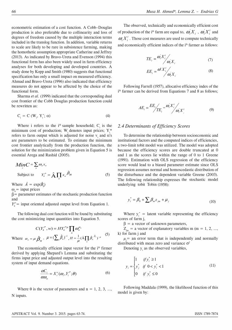
The observed, technically and economically efficient cost

of production of the ith farm are equal to, ii X'ω , t

ii X'ω and

tii X,ω . Those cost measures are used to compute technically

and economically efficient indices of the ith farmer as follows:

)exp( 0BA

=

nω β

*ikY

∏=n

ni

ki



βµ

−∏Α= )ˆˆ(1 ˆn

nnH

);,( * θωαωα i

iiei

n

i YXC=

ii

tii

i XXTE '

'

ωω=

ii

ti

i XXEE '

'ω

ω=

i

ii TE

EEAE = = ti

tii

iX

X'

'

ωω


yi

*

Zjm μj

σ2

(7)

(8)

Following Farrell (1957), allocative efficiency index of the ith farmer can be derived from Equations 7 and 8 as follows;

)exp( 0BA

=

nω β

*ikY

∏=n

ni

ki



βµ

−∏Α= )ˆˆ(1 ˆn

nnH

);,( * θωαωα i

iiei

n

i YXC=

ii

tii

i XXTE '

'

ωω=

ii

ti

i XXEE '

'ω

ω=

i

ii TE

EEAE = = ti

tii

iX

X'

'

ωω


yi

*

Zjm μj

σ2

(9)

2.4 Determinants of Efficiency Scores

To determine the relationship between socioeconomic and institutional factors and the computed indices of efficiencies, a two-limit tobit model was utilized. The model was adopted because the efficiency scores are double truncated at 0 and 1 as the scores lie within the range of 0 to 1 Greene (1991). Estimation with OLS regression of the efficiency score would lead to a biased parameter estimate since OLS regression assumes normal and homoscedastic distribution of the disturbance and the dependent variable Greene (2003). The following relationship expresses the stochastic model underlying tobit Tobin (1958):

)exp( 0BA

=

nω β

*ikY

∏=n

ni

ki



βµ

−∏Α= )ˆˆ(1 ˆn

nnH

);,( * θωαωα i

iiei

n

i YXC=

ii

tii

i XXTE '

'

ωω=

ii

ti

i XXEE '

'ω

ω=

i

ii TE

EEAE = = ti

tii

iX

X'

'

ωω


yi

*

Zjm μj

σ2

(10)

Where yi* = latent variable representing the efficiency

scores of farm j, β = a vector of unknown parameters, Zjm = a vector of explanatory variables m (m = 1, 2, ...,

k) for farm j and μj= an error term that is independently and normally

distributed with mean zero and variance σ2

Denoting yi as the observed variables,

≤

<<

≥

=

00

10

11

*i

*i

*j

*i

i

if y

y if y if y

y

(11)

∏∏∏−−−

′−−

′−

′−=

jijiji Ly

jjjj

yyyy

jjjjjj

ZLZyZLLLZyL

2*

1

2121 11),,.,(

σβ

ϕσβ

φσσ

βϕσβ (12)

(11)

Following Maddala (1999), the likelihood function of this model is given by:



≤

<<

≥

=

00

10

11

*i

*i

*j

*i

i

if y

y if y if y

y

(11)

∏∏∏−−−

′−−

′−

′−=

jijiji Ly

jjjj

yyyy

jjjjjj

ZLZyZLLLZyL

2*

1

2121 11),,.,(

σβ

ϕσβ

φσσ

βϕσβ (12)

(12)

Where L1j = 0 (lower limit), L2j = 1 (upper limit); and φ(.) and ϕ(.) are normal and standard density functions. In practice, since the log function is monotonically increasing function, it is simpler to work with log of likelihood function rather than likelihood function and the maximum values of these two functions are the same Greene (2003).

2.5 Description of the Study Area

This study was undertaken in the central rift valley of Ethiopia, explicitly in Arsi Negelle district. Geographically, the district is located from 380 25’ E to 380 54’ E longitude and 070 09’ to 070 42’ N latitude. Except for the Southeastern part, most of the district’s elevation is between 1500 and 2300 meters. The topography of the area is a gentle slope or flat and the soils of the area are lightweight, friable loam and clay loam. The main crops grown in the area include wheat, maize, teff, barley, sorghum, onion and potato. Annual crops accounted for 95% of all croplands in the district. Andosol soil type covers about 52.2% of the district, while Nitosols cover the remaining 47.8%. The temperature of the area ranges from 16oc to 25oc and annual rainfall ranges between 500-1150 mm. Livestock are an important component of the farming system and a source of intermediate products in the district. The area is intensively cultivated and private grazing land is unavailable. Communal pasture and straw from crops are the main source of feed for livestock production. According to CSA (2012), the district has a total population of 303,223 of which 150,245 are male and 152,978 are females. The average family size for the district was 5.2 (5.3 for urban and 5.1 for rural).

2.6 Sampling Technique and Sample Size

A two stage random sampling technique was used to select sample households for this study. In the first stage, three kebeles that produce maize were selected randomly. In the second stage, 138 sample farmers were selected using a simple random sampling technique from each kebeles proportional to the total number of households of the kebeles.

3. EMPIRICAL RESULT

3.1 Socioeconomic Characteristics of the Sample Respondent

The mean age of the sample farmers was about 42 years with a range of 22 to 70 years. The family size of the sample farmers ranged from one to 13 with a mean of 5.73 person per household. Concerning their literacy level, only 6.52% of the household heads were illiterate while the remaining 93.48% of the respondents were at least capable of reading and writing.

Out of the total sample household heads, 63.04% have attained formal education while 30.43% of them were able to read and write though they did not attain formal education. Regarding the sex of respondents, 93.48% of the sample households were male-headed households.

The minimum land holding of the respondents was 0.50 ha while the maximum size was 4.25 ha. The mean land owned by the sample farmers was 1.81 ha. About 11% of the sample farmers owned land not more than 0.5 ha whereas 18.12% of the sample farmers had more than two ha of land.

The farming system in Ethiopia is mainly based on plough by animal draught power that has created complementarity between crop and livestock production for centuries. About 46% of the sample farmers had a pair of oxen and 12.32% of the sample farmers had two pair of oxen. On average, respondent farmers owned livestock of 8.07 TLU ranging from zero to 81.11 TLU.

The survey result showed that 44.20% of the sample farmers accessed credit from different sources. From the total of sample household interviewed for this study, 47.10% of them indicated that they have received training which is specific to maize production. All of the sample respondents reported that they received extension services though the frequency of contact differs. About 65% of respondents have indicated that they had extension contact on a weekly basis. While nearly a quarter of the sample respondents had contact with extension workers twice a month.

3.2 Econometric Results

3.2.1 Production and Cost Function Parameter Estimates

The dependent variable of the estimated model was maize output (qt) produced in 2011/12 production season and the input variables used in the analysis were area under maize (ha), animal draught power (oxen-days), labour (man-day in man-equivalent), quantity of seed (kg) and inorganic fertilizers specifically DAP and urea (kg). To include those farmers who did not apply DAP and urea in the estimation of the frontier a very small value that approach zero was assigned for non-users of fertilizer.

Prior to model estimation, a test was made for multicollinearity among the explanatory variables using the Variance Inflation Factor (VIF). In a production function analysis, correlation between some of the explanatory variables is expected and collinearity among economic variables is an inherent and age-old problem leading to problems of multicollinearity. However, the values of VIF for all variables entered into the models were below 10 (Appendix Tables 1 and 2), which indicate the absence of multicollinearity among the variables.

Efficiency score are sensitive to specification errors that may lead to hetroskedasticity. As measures of inefficiency in SFA are based on residuals derived from the estimation of a frontier, those residuals are sensitive to specification errors that may passed on to the efficiency scores Hadri et al (2003). Breusch-pagan test was then used to detect the presence of



hetroskedasticity and the test indicated that there was no problem of hetroskedasticity in the models.

The result of the model showed that DAP, area under maize, oxen power, labour and seed had positive and significant effect on the level of output. The increase in these inputs would increase output of maize (Table 2).

Table 1. Estimates of the Cobb Douglas frontier production function

Variables Coefficients Std. Err.

DAP 0.05036*** 0.0077

Urea 0.00471 0.0291

Seed 0.52897*** 0.0843

Land 0.23204** 0.0906

Labour 0.12092* 0.0598

Oxen 0.17006** 0.0595

Constant 1.06943** 0.2988

Lambda 1.94304*** 0. 0520

Sigma square 0.05976*** 0.0125Source: own data

***,** and * represents significant levels at 1%, 5% and 10% respectively

The ratio of the standard error of u (σu) to the standard error of v (σv), known as lambda (λ), is 1.943. Based on λ, gamma (γ) which measures the effect of technical inefficiency in the variation of observed can be derived (i.e. γ= λ2/ [1+λ2]) Bravo-Ureta and Pinheiro (1997). The estimated value of γ is 0.7906 that indicates 79.06% of total variation in farm output is due to technical inefficacy.

The dual frontier cost function derived analytically from the stochastic production frontier shown in Table 2 using Equation 5 is given as:

labouroxuria

dapseedlandii YCωωω

ωωωln109.0ln154.0ln004.0

ln0455.0ln478.0ln2096.0ln903.0087.4ln *

+++

++++=

(13)

Where C is the minimum cost of production of the ith farmer, y* refers to the index of output adjusted for any statistical noise and scale effects and stands for input prices.

3.2.2 Tests of Hypothesis

Before proceeding to the estimation of the parameters from which individual level of efficiencies are estimated, it is essential to examine various assumptions related to the model specification. To do this, two hypotheses were tested. The first test was to verify whether there exists considerable inefficiency among farmers in the production of maize in the study area (to examine whether the average production function (OLS) best fits the data). The other hypothesis that was tested was that all coefficients of the inefficiency effect variables are simultaneously equal to zero. (i.e Ho: = d0 = d1 = d2 … = d13 = 0). The test was done based on the log likelihood ratio test (Table 3) which can be specified as:

labouroxuria

dapseedlandii YCωωω

ωωωln109.0ln154.0ln004.0

ln0455.0ln478.0ln2096.0ln903.0087.4ln *

+++

++++= (13)

[ ][ ])(ln)(ln2

)(/)(ln2

10

10

HLHLHLHLLR

−−=−==

λλ

(14) (15)

The λ value obtained from the log likelihood functions of the average response function and the SFA was found to be greater than the critical value. Hence, the null hypothesis that states the average response function (OLS) is an adequate representation of the data was rejected and the alternative hypothesis that stated there exists considerable inefficiency among sample farmers was accepted. The other hypothesis was also tested in the same way by calculating the λ value using the value of the log likelihood function under the SFA (without explanatory variables of inefficiency effects, (H0)) and the full frontier model with variables that are supposed to determine the inefficiency level of each farmer, (H1). The λ value obtained was again higher than the critical c2 value at the degree of freedom equal to the number of restrictions. As a result, the null hypothesis is rejected in favour of the alternative hypothesis that the explanatory variables associated with the inefficiency effects model are simultaneously different from zero.

3.2.3 Efficiency Scores

The model output presented in Table 3 indicates that farmers in the study area were relatively good in TE than AE or EE. The mean TE was found to be 84.87%. This means in the short run there are opportunities for reducing input used for maize production proportionally by 15.13% to produce the current level of output.

Table 3. Summary of descriptive statistics of efficiency measures

Typ

e of

ef

fici

ency

Min

imum

Max

imum

Mea

n

Std.

D

evia

tion

TE 0.561 0.974 0.84868 0.0819

AE 0.187 0.553 0.37472 0.0555

EE 0.164 0.504 0.31620 0.0456

Source: own data

The mean AE of farmers in the study area was 37.47% indicating there is a need to improve the present level of AE. The estimates depicted that the farmers have ample opportunities to increase their AE. For instance, farmer with an average level of AE would enjoy a cost saving of about 32.24% derived from (1 – 0.37472/0.553)*100 to attain the level of the most efficient farmer.

The mean EE showed that there was a significant level of inefficiency in the production process. That is the producer with an average EE level could reduce current average cost of production by 68.38% to achieve the potential minimum cost level without reducing output levels. It can be inferred that if farmers in the study area were to achieve 100% EE, they would experience substantial production cost saving of



68.38%. This implies that the reduction in cost of production through eliminating resource use inefficiency could add about 68.38% of the production cost to their annual income. The result also indicated that the farmer with an average level of EE would enjoy a cost saving of about 37.26% derived from (1-0.31620/0.504)*100 to attain the level of the most efficient farmer. From these results, it is observable that EE could be improved significantly, and that allocative inefficiency constitutes a more serious problem than technical inefficiency. The level of TE, AE and EE at which sample households operate is presented in Table 4.

3.2.4 Determinants of Efficiency Differentials among Farmers

After measuring levels of efficiency and determining the presence of efficiency difference among farmers, finding out factors causing efficiency disparity among them was the next most important step of this study. To see this, efficiency levels of sample farmers were regressed on factors that were expected to affect efficiency levels. These variables were selected based on previous studies and socioeconomic conditions of the study area (Table 5).

Table 4. Frequency distribution of efficiency estimates of sample farmers

Efficiency level TE AE EE

N Percent N Percent N Percent

00-09.999 0 0.00 0 0.00 0 0.00

10-19.999 0 0.00 1 0.72 3 2.17

20-29.999 0 0.00 5 3.62 44 31.88

30-39.999 0 0.00 94 68.12 87 63.04

40-49.999 0 0.00 35 25.36 3 2.17

50-59.999 1 0.72 3 2.17 1 0.72

60-60.999 8 5.80 0 0.00 0 0.00

70-79.999 22 15.94 0 0.00 0 0.00

80-89.999 62 44.93 0 0.00 0 0.00

90-99.999 45 32.61 0 0.00 0 0.00

Source: own data

Table 5. Maximum likelihood estimates of the tobit model

VariablesTE AE EE

Coef. Std. Err. Coef. Std. Err. Coef. Std. Err.

Education 0.00448 0.00482 0.0087*** 0.0032 0.00937*** 0.00264

Family size(adult-eqt) -0.00363 0.00323 0.0032 0.0022 0.00122 0.00177

Experience 0.00005 0.00062 0.0006 0.0004 0.00052 0.00034

Cultivated land -0.00018 0.00769 -0.0051 0.0051 -0.00415 0.00421

Crop rotation 0.01337 0.01215 -0.0061 0.0081 0.00185 0.00665

Livestock (TLU) 0.00012 0.00090 0.0004 0.0006 0.00037 0.00049

Extension contact 0.00065* 0.00034 -0.0011** 0.0002 -0.00056*** 0.00018

Training -0.01153 0.01394 -0.0074 0.0093 -0.00989 0.00763

Credit 0.04747*** 0.01490 0.0064 0.0100 0.02458*** 0.00815

Distance to market -0.00730** 0.00349 0.0021 0.0023 -0.00126 0.00191

Home to farm distance 0.00418 0.00663 -0.0023 0.0044 0.00002 0.00363

Off/non-farm activity 0.02416 0.01451 -0.0041 0.0097 0.00461 0.00794

Soil fertility 0.00731* 0.01661 0.0097 0.0111 0.00741 0.00909

Cons 0.79409*** 0.03675 0.3806*** 0.0246 0.29721** 0.02012

Source: own data***,** and * represents significant levels at 1%, 5% and 10% respectively



The coefficient for educational level was significant and was positively related to AE and EE at one percent. The positive sign indicates that an increase in human capital enhances the efficiency of farmers. Similar results were obtained in the works of Himayatullah and Imranullah (2011). Ahmed et al. (2001) indicated that education enhances farmers’ ability to interpret and make good use of information about markets and prices in environments.

Frequency of extension contact had significant positive relationship with TE at 10% significance level. The frequent contact facilitates the flow of new ideas between the extension agent and the farmer, thereby giving a room for improvement in farm efficiency. Advisory service rendered to the farmers can help farmers to improve their average performance in the overall farming operation as the service widens the household’s knowledge with regard to the use of productivity and input allocation. This result is also similar to those obtained by Jude et al (2011) and Mbanasor and Kalu (2008). However, the negative coefficient of extension contact, which is significant in AE and EE, indicates that efficiency in resource allocation is deteriorating as the frequency of extension contact increases. This may be due to the fact that extension workers are basically trained to solve the problem of food security and they have limited knowledge for appropriate resource allocation. In addition to this, as Haji (2007) indicated extension workers in the country devotes ample of their time for nonfarm activities such as credit application processing, input distributions and collection of loans and taxes.

The results also indicated that access to credit had a positive and statistically significant effect on both TE and EE at one percent significant level, which indicates that farmers with access to credit tend to exhibit higher levels of efficiency. Credit availability shifts the cash constraint outwards and enables farmers to make timely purchases of those inputs that they cannot provide from their own sources. This result is in line with the argument of Jude et al. (2011).

Distance from home to the nearest market was also significant in determining TE. Farmers far from markets are less technically efficient compared to their counterparts who reside nearby markets. This might be due to the fact that as farmers are located far from the market, there would be limited access to input and output markets and market information. Moreover, higher distance to market leads to higher transaction cost that reduces the benefits that accrue to the farmer. More importantly, longer distance from market discourages farmers from participating in market-oriented production.

The result also indicated that soil fertility was positively and significantly related to TE. This implies that farmers who allocated a land that was relatively fertile were good in TE. Therefore, decline in soil fertility could be taken as cause for significant output loss.

4. CONCLUSIONS AND RECOMMENDATIONS

The result of the analysis showed that maize producers in the study area are not operating at full TE, AE and EE levels and the result indicated that there is opportunity for maize producers to increase output at existing levels of inputs and minimize cost without compromising yield with present technologies available in the hands of producers. Those findings stresses the need for appropriate policy formulation and implementation to enable farmers reduce their inefficiency in production as this is expected to have multiplier effects ranging from farm productivity growth to economic growth and poverty reduction at the macro level.

Education was very important determining factor. Thus, government has to give due attention to training farmers through strengthening and establishing both formal and informal type of framers’ education, farmers’ training centers, technical and vocational schools, as farmer education would reduce both allocative and economic inefficiencies.

The study also revealed that distance to market has a significant influence on the TE of smallholders. Therefore, farmers have to get inputs easily and communication channels have to be improved to get a better level of TE.

Appropriate and adequate extension services should be provided. This could done by designing appropriate capacity building program to train additional development agents to reduce the existing higher ratio of farmers to development agents as well as to provide refreshment training for development agents.

Extension agents have to give due attention for appropriate input allocation and cost minimization in addition to their acknowledgeable effort to increase production. This calls for the need to more effective policy support for extension services and additional efforts need to be devoted to upgrade the skills and knowledge of the extension agents.

Better credit facility has to be produced via the establishment of adequate rural finance institutions and strengthening of the available micro-finance institutions and agricultural cooperatives to assist farmers in terms of financial support through credit are crucial to improve farm productivity.

Farmers have to work to improve the fertility status of the farm. Though it is difficult to achieve this in the short run, farmers can do this by applying fertilizers (organic or inorganic) that are suitable for the farm and practicing soil conservation practices.

Thus, the results of the study give information to policy makers and extension workers on how to better aim efforts to improve farm efficiency as the level and specific determinant for specific efficiency types are identified. This could contribute to compensation of high production cost, hence improve farm revenue, welfare and generally help agricultural as well as economic development. Those findings stresses the need for appropriate policy formulation and implementation to enable farmers reduce their inefficiency in production as this is expected to have multiplier effects ranging from farm productivity growth to economic growth and poverty reduction at macro level.



REFERENCES

Abdourahmane, T., Bravo-Ureta, B., Teodoro, E., 2001. Technical Efficiency in Developing Country Agriculture: A Meta-Analysis. Agricultural Economics, 25: 235-243.

Ahmed, H., Lemma, Z., Endrias, G., 2014. Technical Efficiency of Maize Producing Farmers in Arsi Negelle, Central Rift Valley of Ethiopia: Stochastic Frontier Approach. Agriculture and For-estry, 60 (1): 157-167.

Ahmed, M., Gebremedhin, B., Benin, S., Ehui, S., 2002. Mea-surement of Sources of Technical Efficiency of Land Tenure Con-tracts in Ethiopia. Environmental and Development Economics, 7 (3): 507-527.

Ahmad, M., Bravo-Ureta, B., 1996. Technical Efficiency Mea-sures for Dairy Farms Using Panel Data: A Comparison of Al-ternative Model Specifications. Productivity Analysis, 7:399–416.

Aigner, D., Lovell, C., Schmidt, P., 1977. Formulation and Esti-mation of Stochastic Frontier Production Function Models. Journal of Econometrics, 6: 21–37.

Amin, W., Michael, M., Langemeier, R., 2011. Does Farm Size and Specialization Matter for Productive Efficiency? Results from Kansas. Journal Agricultural and Applied Economics, 43(4):515–528.

Anuradha, N., Zala, y.C., 2010. Technical Efficiency of Rice Farms under Irrigated Conditions in Central Gujarat. Agricultural Economics Research Review, 23: 375-381.

Arega, A., Victor, M., James, G., 2006. The Production Effi-ciency of Intercropping Annual and Perennial Crops in Southern Ethiopia: A Comparison of Distance Functions and Production Frontiers. Agricultural Systems, 91: 51–70.

Arega, D., Rashid, M.H., 2005. The Efficiency of Traditional and Hybrid Maize Production in Eastern Ethiopia: An Extended Ef-ficiency Decomposition Approach. Journal of African Economics, 15: 91-116.

Awudu, A., Hendrik, T., 2007. Estimating Technical Efficiency under Unobserved Heterogeneity with Stochastic Frontier Models: Application to Northern German Dairy Farms. European Review of Agricultural Economics, 34 (3): 393–416.

Battese, G. E., Coelli, T., 1988. Prediction of Firm Level Techni-cal Efficiency with Generalized Frontier Production Function and Panel Data. Journal of Econometrics, 38: 387-399.

Berdiku, q., Gillespie, J., Kenneth, Mc., 2014. Productivity and Efficiency of U.S. Meat Goat Farms: Prepared for the Southern Association of Agricultural Economists Annual Conference, Dal-las, Texas.

Bonabana-Wabbi, J., Mugonola, B., Ajibo, S., Kirinya, J., Kato, E., Kalibwani, R., Kasenge, V., Nyamwaro, S., Tumwesigye, S., Chiuri, W., Mugabo, J., Fungo, B., Tenywa, M., 2011. Agricul-tural Profitability and Technical Efficiency: The Case of Pineapple and Potato in South West Uganda. African Journal of Agricultural and Resource Economics, 8 (3): 145-159.

Boubaker, D., Lassad, L., Mohammed, E., Emna, B., 2007. Mea-suring Irrigation Water Use Efficiency Using Stochastic Produc-tion Frontier: An Application on Citrus Producing Farms in Tu-nisia. African Journal of Agricultural and Resource Economics, 1 (2): 1-15.

Boubaker, D., Haithema, B., Mohamed, A., 2012. Input and Out-put Technical Efficiency and Total Factor Productivity of Wheat Production in Tunisia. African Journal of Agricultural and Re-

source Economics, 7 (1): 70-87.

Bradley, K., Tatjana, H., Mazzanti, R., Charles, E., Wilson, J., Lance, S., 2014. Measurement of Technical, Allocative, Econom-ic, and Scale Efficiency of Rice Production in Arkansas using Data Envelopment Analysis. Journal of Agricultural and Applied Eco-nomics, 46,(1):89–106.

Bravo-Ureta, B.E., Pinheiro, A.E., 1997. Technical, Economic and Allocative Efficiency in Peasant Farming: Evidence from the Dominican Republic. The Developing Economies, 34(1): 48-67.

Bravo- Ureta, B.E., Evenson, E.R., 1994. Efficiency in Agricul-tural Production: The Case of Peasant Farmers in Eastern Para-guay. Agricultural Economics, 10(1): 27-37.

Bravo-Ureta, B. E., Laszlo R., 1991. Dairy Farm Efficiency Mea-surement Using Stochastic Frontiers and Neoclassical Duality. American Journal of Agricultural Economics, 73 (2): 421–28.

Catherine, L., Jeffrey, A., 2013. The Role of Risk Mitigation in Production Efficiency: A Case Study of Potato Cultivation in the Bolivian Andes. Agricultural Economics, 64(2): 363–381.

Cazals, C., Florens, J.P., Simar, L., 2002. Nonparametric Frontier Estimation: A Robust Approach. Journal of Econometrics, 106: 1–25.

Charnes, A., Cooper, W., Rhodes, E., 1978. Measuring the Ef-ficiency of Decision-Making Units. European Journal of Opera-tional Research 2, 429-444.

Coelli, T., Rahman, S., Thirtle, C., 2002. Technical, Allocative, Cost and Scale Efficiencies in Bangladesh Rice Cultivation: A Non-Parametric Approach. Agricultural Economics, 53(3): 607-626.

Coelli, T., Rao D., and Battese, G. E., 1998. An Introduction to Efficiency and Productivity Analysis. Boston, MA: Kluwer Aca-demic Publishers.

Coelli, T., 1995. Recent Development in Frontier Modelling and Efficiency Measurement. Australian Journal of Agricultural Eco-nomics, 39: 219-245.

CSA (Central Statistical Agency), 2012. Statistical Report on Popu-lation Projected Figures for the year 2012, Addis Ababa, Ethiopia.

CSA (Central Statistical Agency), 2011. Statistical Report on Area and Crop Production, Addis Ababa, Ethiopia.

CSA (Central Statistical Agency), 2008. Population and Housing Census Report, Addis Ababa, Ethiopia.

EEA (Ethiopian Economic Association), 2012. Annual Report on Ethiopian Economy. Addis Ababa, Ethiopia.

EEA (Ethiopian Economic Association), 2006. Fourth Annual Re-port on Ethiopian Economy. Addis Ababa, Ethiopia.

Farrell, M.J., Fieldhouse, M., 1962. Estimating Efficient Produc-tion under Increasing Returns to Scale. Journal of the Royal Statis-tical Society, 125: 252 – 267.

Farrell, M. J., 1957. The Measurement of Productive Efficiency, Journal of the Royal Statistical Society, 120:253-281.

Fraser, I., Cordina, D., 1999. An Application of Data Envelopment Analysis to Irrigated Dairy Farms in Northern Victoria, Australia. Agricultural Systems, 59: 267-82.

F€re, R., Grosskopf, S., Lovell, K., 1994. Production Frontiers. Cambridge University Press, Cambridge, 296.

Green, W., 1991. LIMDEP: Users€s Manual and Reference Guide, New york: Econometric Software, Inc.



Greene, W.H., 2003. Econometric Analysis, 5th ed. Pearson Edu-cation Inc., Upper Saddle River, New Jersey.

Gelaw, F., 2013. Inefficiency and Incapability Gaps as Causes of Poverty: A Poverty Line-Augmented Efficiency Analysis Using Stochastic Distance Function. African Journal of Agricultural and Resource Economics, 8(2): 24-68.

Goshu, D., Kassa, B.,Mengistu, K., 2012. Is Food Security En-hanced By Agricultural Technologies In Rural Ethiopia? African Journal of Agricultural and Resource Economics, 8 (1): 58 – 68.

Hadri, K., Guermat, C., Whittaker, J., 2003. Estimating Farm Efficiency In The Presence Of Double Heteroscedasticity Using Panel Data. Journal of Applied Economics, 6(2): 255-268.

Haji, J., 2007. Production Efficiency Of Smallholders’ Vegetable Dominated Mixed Farming System In Eastern Ethiopia: A Non-Parametric Approach. Journal of African Economies, 16(1), 1-27.

Haji, J., Andersson, H., 2006. Determinants of Efficiency of Veg-etable Production in Smallholder Farms: The Case of Ethiopia. Food Economics, 3(3): 125-137.

Hardwick, T., 2009. The Efficiency of Smallholder Agriculture in Malawi. African Journal of Agricultural and Resource Economics, 3 (2):101-121.

Himayatullah, K., Imranullah, S., 2011. Measurement of Tech-nical, Allocative and Economic Efficiency of Tomato Farms in Northern Pakistan. Paper Presented at International Conference on Management, Economics and Social Sciences, Bangkok.

Hjalmarsson, L., Kumbhakar, S., Heshmati, A., 1996. DEA, DFA and SFA: A Comparison. Productivity Analysis, 7: 303-327.

IFPRI (International Food Policy Research Institute), 2010. Maize Value Chain in Ethiopia: Constraints and Opportunities for En-hance the System.

Jean-Paul, C., Ragan, P., Michael, R., 2005. Farm Household Production Efficiency: Evidence from the Gambia. American Journal of Agricultural Economics, 87(1):160–179

Jude, C., Benjamen, C., Patrick, C., 2011. Measurement and De-terminants of Production Efficiency among Smallholder Sweet Po-tato Farmers in Imo State, Nigeria. European Journal of Scientific Research, 59 (3):307-317.

Kalirajan, P., Obwona, B., Zhao, S., 1996. A Decomposition of Total Factor Productivity Growth: The Case of Chinese Agricul-tural Growth Before and After Reforms. American Journal of Ag-ricultural Economics, 78: 331-338.

Karthick, V., Alagumani, T., Amarnath, J., 2013. Resource–Use Efficiency and Technical Efficiency of Turmeric Production in Tamil Nadu: A Stochastic Frontier Approach. Agricultural Eco-nomics Research Review, 26(1): 109-114.

Kassie, M., Holden, S., 2007. Sharecropping Efficiency in Ethi-opia: Threats of Eviction and Kinship. Agricultural Economics, 37:179-188.

Kirkley, E., Squires, D., Strand, E., 1995. Assessing Technical Efficiency in Commercial Fisheries: The Mid-Atlantic Sea Scallop Fishery. American Journal of Agricultural Economics, 77: 686–97.

Kirwan,B.E.,Margaret,M., 2007.Food aid and Poverty.American Journal of Agricultural Economics, 89(5): 1152-1160.

Koopmans, T., 1951. Analysis of Production as an Efficient Com-bination of Activities. Cowles Commission for Research in Eco-nomics, New york, Wiley.

Kopp, J., Smith, K., 1980. Frontier Production Function Estimates for Steam Electric Generation. A Comparative Analysis. Southern Economic Journal, 47: 1049–1059.

Krishna, K., Ashok, M., Samarendu, M., 2014. Determinants of Rice Productivity and Technical Efficiency in the Philippines: Se-lected Paper Prepared for Presentation at the Southern Agricul-tural Economics Association Annual Meeting, Dallas, Texas.

Kularatne, G., Clevo, W., Sean, P., Tim, R., 2012. Factors Af-fecting Technical Efficiency Of Rice Farmers In Village Reservoir Irrigation Systems Of Sri Lanka. Agricultural Economics, 63(3): 627–638.

Kumbhakar, C., Lovell, K., 2000. Stochastic Frontier Analysis. Cambridge University Press, Cambridge.

Maddala, S., 1999. Limited Dependent Variable in Econometrics. Cambridge University Press, New york.

Maddala, G.S., 1999. Limited dependent variable in econometrics. Cambridge University Press, New york.

Matthew, H., Danny, R., 2007. On the Productivity of Public For-ests: A Stochastic Frontier Analysis of Mississippi School Trust Timber Production. Canadian Journal of Agricultural Economics, 55 (2007): 171–183.

Mbanasor, J., Kalu, C., 2008. Economic Efficiency of Commer-cial Vegetable Production System in Akwa Ibom State, Nigeria. Journal of Tropical and Subtropical Agro Ecosystems, 8(3):313-318.

Meeusen, W., Van Den Broeck, J., 1977. Efficiency Estimation from Cobb–Douglas Production Function with Composed Error. International Economic Review, 18:435–444.

Ogunniyi, T., 2008. Profit Efficiency among Cocoa yam Produc-tion in Osun State, Nigeria. International Journal of Agricultural Economics and Rural Development, 1(1), 38-46.

Olesen, O.B., Petersen, N.C., Lovell, K., 1996. Editor’s Introduc-tion. Productivity Analysis, 7:87–98.

Rashid, S., 2010. Staple Food Prices in Ethiopia. Paper Prepared for the COMESA Policy Seminar on Variation in Staple Food Prices: Causes, Consequence, and Policy Options, Maputo, Mo-zambique, the African Agricultural Marketing Project.

Sharma, K., Leung, R, Zaleski, M., 1999. Technical, Alloca-tive and Economic Efficiencies in Swine Production in Hawaii: A Comparison of Parametric and Nonparametric Approaches. Agri-cultural Economics, 20: 23-35.

Seyoum, E.T., Battese, G.E., Fleming, E.M., 1998. Technical Ef-ficiency and Productivity of Maize Producers in Eastern Ethiopia: A Study of Farmers within and Outside the Sasakawa-Global 2000 Project. Agricultural Economics, 19: 341-348.

Simar, L., Wilson, P., 2000. Statistical Inference in Nonparamet-ric Frontier Models: The State of the Art. Productivity Analysis, 13: 49–78.

Spielman, D., Byerlee, D., Avid, J., Alemu, D.,KelemeworkD., 2010. Policies to promote cereal intensification in Ethiopia: The search for appropriate public and private roles. Food Policy, 35: 185-194.

Stefanos, A., Evangelos, P., Zamanidis, S., 2012. Productive Ef-ficiency of Subsidized Organic Alfalfa Farms. Journal of Agricul-tural and Resource Economics, 37(2):280–288.

Tobin, J., 1958: Estimation of relationships for limited dependent variables. Econometrica, 26 (1): 26-36.



Torkamani, J., Hardaker, J., 1996. A Study of Economic Effi-ciency of Iranian Farmers in Ramjerd District: An Application of Stochastic Programming. Agricultural Economics, 14, 73-83.

Udayanganie, A.D., Prasada, D.V., Kodithuwakku, S., Weera-hewa, J., Little, C., 2006. Efficiency of the Agrochemical Input Usage in the Paddy Farming Systems in the Dry Zone of Sri Lan-ka: Prepared for the Annual Meeting of the Canadian Agricul-tural Economics Society, Montreal, quebec.

xu, x., Jeffrey, R., 1998. Efficiency and Technical Progress In and Modern Agriculture: Evidence from Rice Production in Chi-na. Agricultural Economics, 19:157-165.

Appendix Table 1. VIF for the variables entered in to the stochastic frontier model

Variable VIF 1/VIF

Land 8.5 0.117647

Seed 8.32 0.120192

Oxen power 3 0.333333

Labour 2.84 0.352113

DAP 1.42 0.704225

Urea 1.29 0.775194

Mean VIF 4.228333

Appendix Table 2. VLF for the continuous variables entered in to the efficiency model

Variable VIF 1/VIF

cultivated land 2.26 0.442119

Livestock 2.2 0.454481

Family size 1.41 0.71001

Experience 1.27 0.784836

extension contact 1.22 0.820667

distance to mkt 1.22 0.820771

plot to home distance 1.07 0.933107

education 1.04 0.963307

Mean VIF 1.46

Appendix Table 3. Contingency Coefficients of the dummy variables entered in to the efficiency model

Crop rotation Training Credit Soil fertility Off/nonfarm activity

Crop rotation 1.0000

Training -0.0780 1.0000

Credit 0.0104 -0.0341 1.0000

Soil fertility -0.0543 0.0923 0.1514 1.0000

Off/nonfarm activity -0.0950 0.0027 -0.1330 -0.1781 1.0000

doi: 10.19041/apstract/2015/3/9 measuring...

Documents