doi:10.1016/j.jinteco.2005.01.002
DESCRIPTION
* Corresponding author. Gerald R. Ford School of Public Policy, University of Michigan, Lorch Hall, 611 Tappan Street, Ann Arbor, MI 48109-1220, United States. Tel.: +1 734 764 9498; fax: +1 734 763 9181. E-mail addresses: [email protected] (K.M.E. Dominguez), [email protected] (L.L. Tesar). 1 Tel.: +1 734 763 2254; fax: +1 734 764 2769. 1. Introduction Abstract Received 23 November 2001; received in revised form 1 October 2004; accepted 21 January 2005 NBER, United States b a cTRANSCRIPT

Journal of International Economics 68 (2006) 188–218
www.elsevier.com/locate/econbase
Exchange rate exposure
Kathryn M.E. Domingueza,b,c,*, Linda L. Tesarb,c,1
aFord School of Public Policy, University of Michigan, United StatesbNBER, United States
cDepartment of Economics, University of Michigan, Lorch Hall, 611 Tappan Street, Ann Arbor,
MI 48109-1220, United States
Received 23 November 2001; received in revised form 1 October 2004; accepted 21 January 2005
Abstract
In this paper we examine the relationship between exchange rate movements and firm value. We
estimate the exchange rate exposure of publicly listed firms in a sample of eight (non-US)
industrialized and emerging markets. We find that exchange rate movements do matter for a
significant fraction of firms, though which firms are affected and the direction of exposure depends
on the specific exchange rate and varies over time, suggesting that firms dynamically adjust their
behavior in response to exchange rate risk. Exposure is correlated with firm size, multinational
status, foreign sales, international assets, and competitiveness and trade at the industry level.
D 2005 Elsevier B.V. All rights reserved.
Keywords: Firm- and industry-level exposure; Exchange rate risk; Pass-through
JEL classification: F23; F31; G15
1. Introduction
It is widely believed that changes in exchange rates have important implications for
financial decision-making and for the profitability of firms. One of the central
0022-1996/$ -
doi:10.1016/j.j
* Correspond
Tappan Street,
E-mail add1 Tel.: +1 73
see front matter D 2005 Elsevier B.V. All rights reserved.
inteco.2005.01.002
ing author. Gerald R. Ford School of Public Policy, University of Michigan, Lorch Hall, 611
Ann Arbor, MI 48109-1220, United States. Tel.: +1 734 764 9498; fax: +1 734 763 9181.
resses: [email protected] (K.M.E. Dominguez), [email protected] (L.L. Tesar).
4 763 2254; fax: +1 734 764 2769.

K.M.E. Dominguez, L.L. Tesar / Journal of International Economics 68 (2006) 188–218 189
motivations for the creation of the euro was to eliminate exchange rate risk to enable
European firms to operate free from the uncertainties of changes in relative prices
resulting from exchange rate movements. At the macro level, there is evidence that the
creation of such currency unions results in a dramatic increase in bilateral trade
(Frankel and Rose, 2002). But do changes in exchange rates have measurable effects on
firms? The existing literature on the relationship between international stock prices (at
the industry or firm level) and exchange rates finds only weak evidence of systematic
exchange rate exposure (see Doidge et al., 2003; Griffin and Stulz, 2001 for two recent
studies). This is particularly true in studies of US firm share values and exchange
rates.2
The first objective of this paper is to document the extent of exchange rate
exposure in a sample of eight (non-US) industrialized and developing countries over a
relatively long time span (1980–1999) and over a broad sample of firms. We follow
the literature in defining exchange rate exposure as a statistically significant (ex post)
relationship between excess returns at the firm- or industry-level and foreign exchange
returns. A key result from our analysis is the finding that exchange rate exposure
matters for non-US firms. We find that for five of the eight countries in our sample
over 20% of firms are exposed to weekly exchange rate movements and exposure at
the industry level is generally much higher, with over 40% of industries exposed in
Germany, Japan, the Netherlands and the UK.3 We find that there is considerable
heterogeneity in the extent of exposure across our sample of countries as well as large
variation in the direction and magnitude of exposure. Our analysis suggests that exchange
rate movements do matter for a significant fraction of firms, although which firms are
affected and the direction of exposure depends on the specific exchange rate and varies
over time.
Having established that there is a statistically significant relationship between
profitability (as measured by stock returns) and the exchange rate, the second objective
of the paper is to try to explain why some firms are exposed and others are not. We use the
exposure coefficients estimated in the first part of the paper in a set of second-stage
regressions to test three hypotheses about the factors that could explain exposure. The first
hypothesis is that firm characteristics, namely firm size and its industry affiliation, are
correlated with exposure. We find no evidence that exposure is concentrated in a particular
sector, but we do find that small-, rather than large- and medium-sized firms, are more
likely to be exposed. One rationale for this finding could be that larger firms have more
access to mechanisms for hedging exposure than small firms, although data limitations do
not allow us to test this conjecture directly.
Our second hypothesis is that firms engaged in international activities are more
likely to be directly affected by changes in exchange rates. We conjecture that
2 In a sample of US multinational corporations (which are assumed to be the firms most likely to be exposed)
over the period 1971–1987 Jorion (1990) found that only 15 of 287 (5%) had significant exchange rate exposure.
Amihud (1994) found no evidence of significant exchange rate exposure for a sample of the 32 largest US
exporting firms over the period 1982–1988.3 Bodnar and Gentry (1993) test for exchange rate exposure at the industry level in the US, Japan and Canada.
They find significant exposure in 11 of 39 US industries (28%) over the period 1979–1988.

K.M.E. Dominguez, L.L. Tesar / Journal of International Economics 68 (2006) 188–218190
multinational firms, firms with extensive foreign sales and firms with holdings of
international assets are more likely to be exposed to exchange rate movements, and
that they are likely to benefit from a depreciation of their home currency. In France,
Germany, Japan and the UK we find evidence that measures of a firm’s international
activities are linked to exposure and the coefficient on the direction of exposure is
indeed positive.
Our third hypothesis is that firms engaged in trade are more likely to face exchange
rate risk. Here, the direction of the exposure is more complicated. Exporting firms may
benefit from a depreciation of the local currency if its products subsequently become
more affordable to foreign consumers. On the other hand, firms that rely on imported
intermediate products may see their profits shrink as a consequence of increasing costs
of production due to a depreciating currency. One might expect, then, to find a
correlation between exposure (positive or negative) and a firm’s engagement in
international markets. Lacking firm-level data on exports and imports, we use a number
of proxies for a firm’s relationship with international markets to test this hypothesis. We
group firms into traded and nontraded sectoral categories to see if exposure is more
concentrated in firms in the traded sector. Finally, we use data on bilateral trade flows at
the industry level to examine the link between firm-level returns and bilateral, industry-
level trade flows.
Even firms that do no international business directly, however, could be affected
by the exchange rate through competition with foreign firms. For example, if Ford
Motor Company were to sell no cars abroad nor import any foreign auto parts,
domestic automobile sales would still be affected if the dollar price of competing
Japanese automobile imports falls or rises. We posit that exposure could depend on
the competitiveness of a particular industry—in less competitive industries, prices are
set farther from marginal cost implying higher mark-ups. In such industries firms
will have some ability to absorb exchange rate changes by adjusting profit margins
and lowering bpass throughQ. In more competitive industries we might expect close
to perfect pass-through and therefore larger effects of exchange rate movements on
stock returns.4 To test this hypothesis we examine the link between firm-level exposure
and two OECD measures of market concentration, a Herfindahl index and a mark-up
index.
On a country-by-country basis we find only weak evidence that measures of trade and
the degree of competitiveness of a particular industry are linked to firm-level exposure.
Note that all of our measures used to test this hypothesis are industry-level indicators. It
could be that there is sufficient heterogeneity in the trading patterns of firms within an
industry that our industry-level variables simply do not reflect the impact of trade at the
firm level. In our cross-country regressions, we find the industry-level export and import
variables enter significantly and are correctly signed, suggesting that the additional
4 Bodnar et al. (2002) and Marston (2001) develop a framework for analyzing the joint phenomena of pass-
through and exposure. Nucci and Pozzolo (2001) examine the impact of exchange rate fluctuations on investment
in a sample of Italian manufacturing firms and find a link between monopoly power and the impact of exchange
rate effects. Allayannis and Ihrig (2000), Campa and Goldberg (1995, 1999) and Dekle (2000) also find a
relationship between market structure and exposure.

K.M.E. Dominguez, L.L. Tesar / Journal of International Economics 68 (2006) 188–218 191
variation in the cross-country trade data helps us better identify exposed firms. We also
find that the Herfindahl index enters significantly in the cross-country regression;
however, the sign on the coefficient indicates that firms in more concentrated industries are
more exposed.5
Taken as a whole, our findings suggest that a significant fraction of firms are exposed to
exchange rate risk in our sample of countries, but which firms are exposed changes over
time. We do find a link between international activity and exposure, but for the vast
majority of firms we are unable to identify the factors that account for their exposure. At
first pass, this would seem to be a puzzling finding. If exchange rate movements matter for
firms, why is it so difficult to identify the determinants of that exposure? On deeper
reflection, however, it is not clear that there is a puzzle after all. Exchange rate exposure,
as measured by the co-movement between exchange rates and excess returns, incorporates
the effects of any hedging activity undertaken by the firm. Firms may use financial
derivatives to help insure against exchange rate risk, or they may manage risk
operationally by importing intermediate inputs from a number of suppliers, or by selling
to an internationally-diversified consumer market.6 Indeed the finding that the subset of
firms exposed to exchange rate movements is not stable over time is likely an indication
that firms dynamically adjust their behavior in response to exchange rate risk. Viewed
from this perspective, it would perhaps have been more puzzling to have identified a set of
firms whose profits were consistently affected by movements of a particular exchange rate
over a long span of time.7
The paper is organized as follows. The definition of exchange rate exposure is covered
in Section 2 and Section 3 describes our dataset. The benchmark exposure results and the
robustness of these results are discussed in Section 4. The second-stage results on the links
between exchange rate exposure and other factors are reported in Section 5. Section 6
concludes.
2. Defining exchange rate exposure
We follow the extensive literature on foreign exchange rate exposure by defining
exposure as the relationship between excess returns and the change in the exchange rate
5 A positive coefficient on the Herfindahl index is puzzling because we would expect firms in less competitive
industries to have lower exchange rate pass through. It may be, however, that the Herfindahl index in this context
is picking up the small firm size effect. Recall that our Herfindahl indices are only available at the industry level.
It may be that industries with high Herfindahl indices are made up of a few large firms and a number of smaller
firms. Our coding assigns the same Herfindahl index to both sets of firms (in the same industry), suggesting that
our positive coefficient may be driven by the small (competitive) firms assigned to high Herfindahls.6 Bodnar and Marston (2001) find that foreign exchange exposure is low for a sample of 103 US firms that
answered their survey of derivative usage. On the other hand, survey results reported in Loderer and Pichler
(2000) suggest that Swiss firms do not seem to know the extent of their cash-flow exposure to exchange rate risk.
And, based on surveys, Bodnar et al. (1998) find that firms do not seem to use derivatives to hedge exchange rate
risk and in many instances, appear to use derivatives to take open positions with respect to the exchange rate.7 To be clear, persistent ex post exchange rate exposure should not be interpreted as evidence against market
efficiency because idiosyncratic exchange rate risk could still be diversified away by individual investors.

K.M.E. Dominguez, L.L. Tesar / Journal of International Economics 68 (2006) 188–218192
(Adler and Dumas, 1984). More formally, we measure exposure as the value of b2,i
resulting from the following two-factor regression specification:
Ri;t ¼ b0;i þ b1;iRm;t þ b2;iDst þ ei;t ð1Þ
where Ri,t is the return on firm i at time t, Rm,t is the return on the market portfolio, b1,i is
the firm’s market beta and Dst is the change in the relevant exchange rate. Under this
definition, the coefficient b2,i reflects the change in returns that can be explained by
movements in the exchange rate after conditioning on the market return. Exposure in this
context is defined as marginal in the sense that each firm’s exposure is measured relative to
the market average.8
Note that a literal interpretation of the CAPM suggests that in equilibrium, only market
risk should be relevant to a firm’s asset price, and therefore only changes in the market
return should be systematically related to firm returns (Ri,t). If the CAPM were the true
model for asset pricing, the coefficient on the change in the exchange rate, b2,i, should be
equal to zero and evidence that b2,i is non-zero could be interpreted as evidence against the
joint hypothesis that the CAPM holds (i.e. the market efficiently prices systematic risk)
and that exchange rate risk is unimportant for stock returns. In this paper, we are not
interested in testing a specific version of the CAPM, nor are we testing whether exchange
rate risk is bpricedQ. Our approach is to use the market model (Eq. (1)) as a framework for
isolating the relationship between excess returns and exchange rates in a cross-section of
firms. In the second stage of our analysis (Section 5), we will try to link the estimated
exchange rate bbetasQ with a set of factors that could proxy for plausible channels for
exposure.
3. The data set
Our dataset includes firm-, industry- and market-level returns and exchange rates for
a sample of eight countries including Chile, France, Germany, Italy, Japan, the
Netherlands, Thailand and the United Kingdom over the 1980–1999 period. The
specific countries in our sample were chosen both on the basis of data availability and
to include in our sample both OECD and developing countries. Returns are weekly
(observations are sampled on Wednesdays) and are taken from Datastream. For
countries with a large number of publicly traded firms (in our sample these include
Germany, Japan and the United Kingdom) we select a representative sample of firms
(25% of the population) based on market capitalization and industry affiliation. For the
remaining countries we include the population of firms. Table 1 provides summary
information on the degree of data coverage across the eight countries. Our sample
includes 2387 firms. On average the sample includes 300 firms for each country; the
8 An alternative approach is to measure total exposure, or the unconditional correlation of exchange rates and
returns. The advantage of total exposure is that it allows one to measure the exposure of all firms as a group,
rather than individual firms relative to the country average. The disadvantage of total exposure is that it does not
allow one to distinguish between the direct effects of exchange rate changes and the effects of macroeconomic
shocks that simultaneously affect firm value and exchange rates.

Table 1
Data coverage
Chile France Germany Italy Japan Neth Thailand UK
1. Coverage of population of firms
# of firms in sample 199 228 204 278 488 213 389 388
# of firms in population 225 228 897 301 1942 248 409 1550
% coverage 88.4 100 22.7 92.4 25.1 85.9 95.1 25
2. Coverage of industries
# of industry indices 23 36 34 31 36 29 20 39
% coverage 100 100 100 100 100 100 100 100
3. Multinational status
# of MNCs in our sample 0 33 27 21 64 16 0 47
% of firms 0 14.5 13.2 7.6 13.1 7.5 0 12.1
4. Trade data
Industry-level bilateral trade yes yes yes yes yes yes yes yes
Trade concentration shares no no no no yes no no yes
5. Market concentration indices
Industry-level Herfindahl index no yes yes no yes no no yes
Industry-level Mark-up index no yes yes yes yes yes no yes
6. International asset data
% of firms reporting during 1996–1999 12.1 21.9 9.8 25.9 69.5 17.8 53.2 70.1
% of firms reporting non-zero values 0 6 9.8 0.4 26.2 9.4 3.9 36.6
7. Foreign sales data
% of firms reporting during 1996–1999 13.6 53.5 58.8 70.1 75.2 59.6 54.8 76
% of firms reporting non-zero values 3 39.4 39.2 49.3 33.8 53.1 5.9 46.1
Firm- and industry-level returns are Wednesday returns from Datastream in local currencies. Firms are sampled based
on industry affiliation and firm size. Industry returns are at the 4-digit level.Multinational status is based on inclusion in
(1) Worldwide Branch Locations of Multinationals (1994), (2) Directory of Multinationals (1998), or (3) the Financial
TimesMultinationals Index. Industry-level bilateral trade data are from Feenstra (2000). Market concentration data are
OECD Secretariat calculations for 1990. Trade concentration shares are from Campa and Goldberg (1997).
International asset and foreign sales data are annual averages over the period 1996–1999 from Worldscope.
K.M.E. Dominguez, L.L. Tesar / Journal of International Economics 68 (2006) 188–218 193
largest fraction of firms in the total sample are Japanese firms (20%), and the smallest
fraction are Chilean (8%). Firms with fewer than 6 months of data during the period
1980–1999 were excluded from our sample.
In Section 5 of the paper, we attempt to link our estimates of exposure to variables such
as industry affiliation, firm size, a firm’s multinational status, information on trade,
industry-level market concentration and a firm’s holdings of international assets and its
foreign sales. Parts 2 through 6 of Table 1 provide information about the coverage of these
variables. Datastream provides industry-level returns at a fairly disaggregated level (we
focus on the 4-digit level). As shown in the second part of Table 1, there are between 23
and 39 industry categories across our sample of countries. (The list of industries is
provided in Appendix Table A1).
Information about multinational status comes from three sources. The first source is
Worldwide Branch Locations of Multinationals (1994), which includes a sample of 500
companies that have foreign branches. The second source, The Directory of Multinationals
(1998), includes the 500 largest firms with consolidated sales in excess of $US 1 billion
and overseas sales in excess of $US 500 million in 1996. Our third source of multinational
information comes from the Financial Times Multinational Index (created in 2000). If a

K.M.E. Dominguez, L.L. Tesar / Journal of International Economics 68 (2006) 188–218194
firm appeared as a multinational in any of the three sources, we coded that firm as a
multinational.
We draw on two sources to gather information about trade, both of which provide data
only at the industry level. The first is Feenstra’s (2000) database on world bilateral trade
flows over the 1980–1997 period. This data source allows us to identify each country’s
major bilateral trading partners by industry. As shown in part 4 of Table 1, the Feenstra
database covers all of the countries in our sample, although it does not cover all of the
industry categories available from Datastream. The second source of trade information is
the export, import and net input shares in manufacturing industries reported by Campa and
Goldberg (1997). Their study covers two of the countries in our sample, Japan and the
United Kingdom.
We are able to test whether exposure is related to industry level market structure using
two measures of market concentration, both based on OECD data. The Herfindahl index,
commonly used to rank the competitiveness of industries, is calculated as the sum of the
squares of the market shares of all firms in an industry (these are OECD Secretariat
calculations for 1990 based on the STAN database). Our second measure of industry
structure is a mark-up index estimated by Oliveira Martins et al. (1996) based on the
method suggested by Roeger (1995). As shown in part 5 of Table 1, the mark-up measure
is available for all the countries in our sample except Chile and Thailand and the
Herfindahl index is also unavailable for Italy and the Netherlands.
While Datastream provides information about industry affiliation and market
capitalization for all firms in our dataset, the coverage ratios for international asset and
foreign sales9 data (available through Worldscope) is more limited. In the regression
analysis below we use annual values of foreign sales and international assets averaged
over the period 1996–1999. As shown in parts 6 and 7 of Table 1, the number of firms that
report international assets and/or foreign sales varies considerably from country to country.
Over 50% of Japanese and UK firms provide these data, while only 3% of Chilean firms
(the country with the lowest coverage) provided non-zero foreign sales data and no
Chilean firms provided non-zero international asset data. Worldscope codes firms that do
not provide international asset or foreign sales data in two ways, with either a missing
value code or a zero. Unfortunately the decision about whether to code a firm without data
as missing or with a zero is apparently arbitrary. Firms that do provide information,
however, also may genuinely have no foreign sales or international assets. This means that
both a zero and a missing value code provide ambiguous information. If one looks only at
those firms that report non-zero, and therefore unambiguous information, about foreign
sales and international assets, the percent of the sample reporting drops dramatically,
especially for international assets. Less than 10% of firms report non-zero international
assets in Chile, France, Germany, Italy, Netherlands and Thailand. In Japan and the UK,
the share of firms reporting any data on international assets is about 70%, and drops to less
than 40% if we only use non-zero values.
9 Foreign sales are defined as sales by foreign affiliates, not the total sales of the firm to foreign markets. These
data have been found to be good indicators of exposure in a number of previous studies, including Doidge et al.
(2003), He and Ng (1998), Frennberg (1994) and Jorion (1990).

K.M.E. Dominguez, L.L. Tesar / Journal of International Economics 68 (2006) 188–218 195
4. The extent and robustness of foreign exchange exposure
We begin by running a benchmark specification for exposure where the independent
variable is weekly firm- (or industry-) level returns and the right-hand-side variables are
the equally-weighted local market return for each country10 and the change in the
exchange rate. One of the first problems that arises when thinking about exchange rate
exposure is bWhich is the relevant exchange rate?Q. Many, if not most studies use the
trade-weighted exchange rate to measure exposure.11 As Williamson (2001) notes, the
main shortcoming of using a trade-weighted basket of currencies in exposure tests is that
the results lack power if a firm is mostly exposed to a small number of currencies. For
instance, if a firm is exposed to only one or a few of the currencies within the basket, this
may lead to an underestimation of the exposure of the firm. One possible research strategy
to mitigate this problem is to create firm- and industry-specific exchange rates. The
difficulty with this approach is that it is not clear on what basis these exchange rates should
be chosen. As we will show below, firms within the same industry have very different
exposure coefficients, suggesting that one needs detailed firm-specific data to isolate
which exchange rate is relevant for capturing exchange risk.
Fig. 1a and b show the benchmark results for firm- and industry-level exposure across
the eight countries using three different currencies: the trade-weighted exchange rate (in
large part to compare our results with those in the literature), the dollar exchange rate, and
one additional bilateral exchange rate based on the country’s direction of trade data.12 The
bars in the plots show the percentages of firms (Fig. 1a) and industries (Fig. 1b) in the
sample with significant (at the 5% level using robust standard errors) exposure using each
of the three currencies. The bar labeled bany exchange rateQ is the percentage of industriesor firms that have significant exposure at the 5% level to at least one of the three listed
exchange rates. Note that exposure to bany exchange rateQ is an indirect measure of the
correlation between the three currencies. If the correlation between the three currencies
were zero, exposure to any of the three would simply be the sum of the exposure to the
three currencies separately. The scale across Fig. 1a and b is the same to make the
comparison between industry- and firm-level exposure easier.
Focusing first on exposure at the firm level, we find that the percent of firms exposed to
any of the three exchange rates ranges from a minimum of 14% in Chile to a maximum of
31% in Japan. Looking across countries, in five of the eight countries over 20% of firms
exhibit significant exposure, a result that differs markedly from the low levels of exposure
found in studies of US firms. Fig. 1b shows the sensitivity of exposure to the three
different exchange rates at the industry-level. The extent of exposure is significantly higher
10 In robustness checks, we compare results using the value-weighted local index and the international index as
alternatives to the equally-weighted index. See Fig. 3 below.11 Three exceptions are Williamson (2001), Dominguez (1998) and Dominguez and Tesar (2001a). Doidge et al.
(2003) use both bilateral rates and trade-weighted exchange rates but bscoreQ total exposure based on one rate.12 The country’s bmajor trading partnerQ is the country with the most trade with the reference country, where
trade is defined as the average of exports plus imports in the 1990s. Trade data are taken from the Direction of
Trade statistics reported by the International Monetary Fund. If the US is the country’s major trading partner, the
currency of the second largest trading country is used.

0
10
20
30
40
50
60
70
Chile France Germany Italy Japan Neth Thailand UK
Per
cent
of f
irms
expo
sed
at th
e 5%
leve
l
Any exch rate Trade-weighted exch rate US dollar Currency of major trading partner
b
a
0
10
20
30
40
50
60
70
Chile France Germany Italy Japan Neth Thailand UK
Per
cent
of i
ndus
trie
s ex
pose
d at
the
5% le
vel
Any exch rate Trade-weighted exch rate US dollar Currency of major trading partner
Fig. 1. (a) Firm-level exposure to different exchange rates. Percentages are based on the number of firms in that
country with a significant coefficient on the exchange rate in Eq. (1) using robust standard errors and
conditioning on the local market index. Exposure to bany exchange rateQ indicates the percent of firms for which
any of the three exchange rates (trade-weighted, US$ and currency of major trading partner) is significant at the
5% level. (b) Industry-level exposure to different exchange rates. Percentages are based on the number of
industries in that country with a significant coefficient on the exchange rate in Eq. (1) using robust standard errors
and conditioning on the local market index. Exposure to bany exchange rateQ indicates the percent of industries
for which any of the three exchange rates (trade-weighted, US$ and currency of major trading partner) is
significant at the 5% level.
K.M.E. Dominguez, L.L. Tesar / Journal of International Economics 68 (2006) 188–218196

K.M.E. Dominguez, L.L. Tesar / Journal of International Economics 68 (2006) 188–218 197
at the industry level for all the countries, though particularly so for Germany, Japan, the
Netherlands and the UK. Over 50% of Japanese industries exhibit significant exposure to
the dollar (and the trade-weighted exchange rate). The high level of dollar exposure in
Japan is consistent with the fact that most exporting firms in Japan invoice their sales in
dollars.13
Since much of the literature has focused on exposure to the traded-weighted exchange
rate, it is interesting to ask whether exposure to the trade-weighted exchange rate differs
from results using a bilateral rate. To get at this question, we calculate the percent of times
a firm is exposed to the dollar, but is not exposed to the country’s trade-weighted exchange
rate. This percentage varies from 15% in Thailand, to 39% in the UK, 65% in France, and
86% in Chile. We take this as an indication that the trade-weighted exchange rate, taken
alone, may not be a good indicator of overall exposure for many countries.
It could still be the case that the restriction to the three exchange rates in Fig. 1a and b
still misses the exchange rate that is most relevant for a given firm. While we do not have
enough information at the firm level to identify the brightQ firm-level exchange rate, we
can form industry-specific exchange rates based on industry-level trade flows. Although
firm-level export and import data is not available for a large sample of firms, information
on industry-level international trade is available in Feenstra’s (2000) World Trade Flows
database. Rather than include the same exchange rate for all firms in a country as we did in
Fig. 1a and b, we can now use an exchange rate that reflects industry-level bilateral trade
flows. These data will only be a good proxy for firm-level trade flows in industries where
trade patterns at the firm level are similar across firms within the same industry. For
example, the country that imports the largest fraction of Japanese automobiles is the
United States, suggesting that the appropriate currency to include in the exposure
regression for Japanese firms in the automotive industry is the US dollar. If, however,
some firms in the Japanese automotive industry specialize in sales to the UK and not the
United States, the regression coefficient will only pick up exposure to the extent that the
dollar–yen rate is correlated with the pound–yen rate.
Fig. 2 presents the percentages of firms that are significantly exposed to these industry-
specific trade-based exchange rates.14 The scale is set to be the same as in Fig. 1a and b for
easy comparison. Interestingly the results using both the industry-specific leading export
country currencies and the industry-specific leading import country currencies do not
differ significantly from the exposure levels we find when we use the dollar rate for all the
firms.15 The fact that the trade-based currency does not identify more exposure could be
due to two reasons. The first could be that a firm’s engagement in international trade
simply doesn’t increase a firm’s exposure to exchange rate movements—firms either
hedge the effects of exchange rate changes, or the exchange rate movements are not the
key factor affecting profitability. The second explanation could be that trade does indeed
result in exposure to exchange rate movements, but the industry-level exchange rate is
13 See Dominguez (1998) for further discussion of the link between exposure and invoicing in Japan.14 We include results based on just the top export or import country’s currency. We also examined exposure to a
basket of the top three trade partners’ currency and found little difference in the results.15 The industry-specific trade data were not available for all the Datastream industries, therefore the exposure
estimates in Fig. 2 are based on the subsample of firms in industries for which we have the trade data.

0
10
20
30
40
50
60
70
Chile France Germany Italy Japan Neth Thailand UK
Per
cent
of f
irms
expo
sed
at th
e 5%
leve
l
Currency of industry exports Currency of industry imports
Fig. 2. Firm-level exposure to trade-based industry-specific exchange rates. Percentages are based on the number
of firms in that country with a significant coefficient on the exchange rate in Eq. (1) using robust standard errors
and conditioning on the local market index. The exchange rates are the currencies of the country’s top trading
partner by industry. The first bar shows the percent of firms exposed to the currency of its industry’s top market
for exports. The second bar shows the percent of firms exposed to the currency of its industry’s top source of
imports. Firms are assigned an industry affiliation according to Datastream. Industry-level trade data are from
Feenstra (2000).
K.M.E. Dominguez, L.L. Tesar / Journal of International Economics 68 (2006) 188–218198
misspecified. Although we do not have good data on firm-level trade, we do know that on
average, about half of the exposure betas in a given industry are negative and about half
are positive, suggesting considerable heterogeneity across firms’ exposure even within an
industry.16 Whatever the true explanation, the fact that we do not find that firm-level
exposure increases when we use a trade-based currency in the benchmark regression
suggests that we are unlikely to find a strong connection between trade and exposure in
our second-stage analysis below.17
4.1. Specification of market index
Our measure of marginal exposure, which is the one typically used in the literature,
reflects the relationship between returns and exchange rates after conditioning on the
market. There are two issues that arise when estimating marginal exposure. The first has to
do with which market index one should use to proxy for bthe marketQ. Empirical tests of
the standard CAPM model typically include the return on the value-weighted market
16 Examples of studies in the literature that test for exposure at the industry level include Allayannis (1997),
Allayannis and Ihrig (2000), Bodnar and Gentry (1993), Campa and Goldberg (1995) and Griffin and Stulz
(2001).17 Forbes (2002) examines the connection between trade linkages and country vulnerability to currency crises for
a sample of developing countries. In future work we hope to explore the relationships between the ex ante
magnitude of firm level exposures in (currency) crisis and non-crisis countries.

K.M.E. Dominguez, L.L. Tesar / Journal of International Economics 68 (2006) 188–218 199
rather than the equally-weighted market. Bodnar and Wong (2003), however, argue that
the value-weighted market return is dominated by large firms that are more likely to be
involved in international activity and as a consequence are more likely to experience
negative cash flow reactions to dollar appreciations than other US firms. Therefore,
including the value-weighted return in an exposure test not only removes the
bmacroeconomicQ effects, but also the more negative effect of exchange rates on cash
flow in larger firms. This would likely bias tests toward finding no exposure. Alternatively,
one could argue that in a world of perfectly integrated capital markets the bmarket returnQmight better be proxied by a global portfolio of stocks rather than a national portfolio.
To sort out the impact of the choice of market index on exposure, Fig. 3 shows the
percent of firms in each country with a significant exposure to the US dollar under
different specifications of the market index. In general the difference in the amount of
estimated exposure across the equally-weighted and the value-weighted specification is
slight; in some countries (France, Germany and the UK) there is slightly more evidence of
exposure when the value-weighted index is used, and in other countries (Italy, Japan and
Thailand) there is slightly more exposure with the equally-weighted index. Because the
results using the equally-weighted and the value-weighted market indices are so similar,
we will use the equally-weighted index in the remaining analysis.
The third bar for each country in Fig. 3 allows for a comparison of the incidence of
exposure across the specifications using the local market indices and the international
index. The international index is the World index reported by Datastream converted to the
reference country’s currency. The percentage of firms found to be significantly exposed
0
10
20
30
40
50
60
70
80
C
Per
cent
of f
irms
expo
sed
at th
e 5%
leve
l
Equally weighted market index Value weighted market index International index
Fig. 3. Sensitivity of firm-level dollar exposure to different market indices. Percentages are based on the number
of firms in that country with a significant coefficient (at the 5% level) on the exchange rate in Eq. (1) using robust
standard errors and conditioning on one of three market indices. The exchange rate in all regressions is the
bilateral rate with the US dollar. All regressions include one of: the equally-weighted local market index, the
value-weighted local market index or the international index.

K.M.E. Dominguez, L.L. Tesar / Journal of International Economics 68 (2006) 188–218200
when conditioning on the international index is now substantially higher, with over 20% of
firms in all eight countries exposed, and over 70% of firms exposed in Japan and the UK.
The likely reason for the increase in the significance of the exchange rate in the benchmark
regression is due to the fact that the international index does a poor job of explaining
returns. The average adjusted-R2 in the regression using the international index falls
relative to the adjusted-R2 when the local market index is used, in some cases by 50% or
more.18 Thus, more firms appear to be exposed simply because the exchange rate is
picking up more of the variability of returns and the market is picking up substantially less.
It is also the case that correlations between the international index and changes in the
relevant exchange rate are generally high (ranging from 0.22 to 0.48) suggesting that
multicollinearity may be a problem.19 In the remaining tests, we will use the local rather
than the international index as our conditioning variable, though it is worth noting that this
may downward bias our estimates of exposure.20
Another potential problem with conditioning on the market is that, in cases where the
market index as a whole is correlated with the exchange rate, marginal firm-level exposure
will appear to be small even though aggregate market-level exposure is high. Conceivably
some of the relatively lower levels of exposure, for example in our two developing
countries, found in Figs. 1a,b and 2 could be explained by high correlations between the
market index and exchange rates. We did not find convincing evidence that this is the case.
In general, correlations between market indices and exchange rates are small and vary
considerably across countries and over time. For example, over the full sample of data
(1980–1999) the weekly correlation between the equally-weighted market index and the
bilateral exchange rate with the dollar ranges from small and negative (Thailand, �0.15;
Japan, �0.07; Chile, �0.001) to small and positive (Germany, 0.12; Netherlands, 0.25).21
As a consequence, the reported levels of exposure are unlikely to be biased downward
because the market index is absorbing the impact of movements in the exchange rate.
4.2. Sensitivity of exposure to horizon
Several studies of exposure have found that the extent of estimated exposure is
increasing in the return horizon (see, for example, Bartov and Bodnar, 1994; Allayannis,
1997; Bodnar and Wong, 2003; Chow et al., 1997a,b). Indeed, most studies of exposure
are conducted using monthly returns, suggesting that our results based on weekly returns
18 As in most CAPM regressions, the R2’s are small under any specification. The key point here is that the
explanatory power of the regression is much smaller when the international index is used. We do not report the
R2’s here but they are available upon request.19 An international index, by its very nature, will be correlated with exchange rates given that it contains returns
for various countries which then all need to be translated into one currency.
21 For completeness, we examined the correlation between the market index (equally-weighted and value-
weighted) and the exchange rate (trade-weighted, US dollar, and currency of major trading partner) over the full
time period and over various subperiods. Although there were some instances when the correlation was
significantly different from zero, no consistent relationship between a particular exchange rate and the market
index emerged that would lead to a serious underestimation of exposure based on Eq. (1).
20 Connolly et al. (2000) indirectly measure exposure by testing whether the relevant regional or country indices
outperform the international index in explaining cross-country firm-level returns.

0
10
20
30
40
50
60
70
C
Per
cent
of f
irm
s ex
pose
d at
the
5% le
vel
1 week 4 weeks 12 weeks 24 weeks 52 weeks
Fig. 4. Sensitivity of firm-level dollar exposure to the return horizon. Percentages are based on the number of
firms in that country with a significant coefficient (at the 5% level) on the exchange rate in Eq. (1) using robust
standard errors and conditioning on the equally-weighted local market index. The exchange rate is US dollar
exchange rate. Returns are based on rolling regressions using 1-week, 4-week, 12-week, 24-week and 52-week
lengths estimated with GMM, correcting for serial correlation.
K.M.E. Dominguez, L.L. Tesar / Journal of International Economics 68 (2006) 188–218 201
may understate the true extent of exposure. Fig. 4 shows the percent of firms with
significant US dollar exposure in our eight-country sample at the 1-, 4-, 12-, 24- and 52-
week return horizons. The results are based on rolling regressions estimated by GMM,
correcting for serial correlation. Consistent with the literature, we find that exposure is
indeed increasing in the return horizon for most firms in our sample. Exposure in Chile
stands out as the most extreme case. Using weekly returns, less than 4% of Chilean firms
appeared to be exposed to the US dollar. That fraction increased to 30% at the quarterly
horizon and to 39% at the yearly horizon. Japan is the only country in the sample where
exposure peaks at the quarterly horizon.22
The fact that exposure increases with the return horizon raises the possibility that the
second-stage regressions might be more successful in explaining exposure if one were to
use exposure coefficients based on monthly or quarterly data. Repeating the second-stage
regressions for Chile and Italy (the two countries with the largest increase in exposure
level with an increase in horizon) and the UK and Japan (the countries with the most
significant exposure over all horizons), with monthly and quarterly exposure coefficients,
however, did not change the qualitative conclusions we report below. Analysis of the beta
estimates for firms in these countries indicates that there is quite a bit of variation in both
the magnitude and sign of betas across the three return horizons. However, there is little
beta variation for those firms with significant exposure betas across all three horizons—
22 Analysis of the beta coefficients at different horizons suggests that the magnitude, statistical significance, and
in many cases the sign of a firm’s exposure coefficient changes across different horizons.

K.M.E. Dominguez, L.L. Tesar / Journal of International Economics 68 (2006) 188–218202
suggesting that it is these firms in the second stage cross-section that are driving the
results. Thus, we will continue to use exposure estimates based on weekly returns in the
second-stage analysis below.
4.3. Magnitude and direction of exposure
Table 2 provides summary information on the sign and the magnitude of the exposure
coefficients. Part A of Table 2 reports the percent of exposure coefficients that are positive
and the percent that are negative. Currencies are measured in units of the reference
country’s currency per foreign currency (TW, $US or major trading partner). In regressions
that include changes in the trade-weighted exchange rate three of the countries (Chile,
Germany and Italy) have about evenly split positive and negative exposure. In another four
countries (France, Japan, the Netherlands and the UK) 60–70% of firms exhibit positive
exposure (meaning that a depreciation of the home currency results in an increase in firm
share value). In Thailand, 79% of exposed firms have negative exposure coefficients,
Table 2
Direction and magnitude of FX exposure
Chile France Germany Italy Japan Neth Thailand UK
A. Direction of exposure
1. TW exchange rate
% positive 50 61 54 53 62 63 21 70
2. $US
% positive 43 53 43 54 47 42 25 45
B. Average increase in R2 (in percent)
1. Across all firms
tw exchange rate �0.017 0.015 �0.028 0.150 0.250 0.141 0.632 0.077
US$ 0.015 �0.001 �0.004 0.031 0.233 0.178 0.707 0.083
Major trading partner 1.469 0.023 �0.004 0.218 0.507 0.143 0.380 0.041
2. At 5% level of significance
tw exchange rate 0.851 1.060 0.418 1.099 0.924 1.187 2.641 1.119
US$ 2.512 1.171 0.480 0.975 1.111 1.271 2.837 1.147
Major trading partner 1.469 1.234 0.471 1.017 1.207 1.363 2.243 1.159
C. Average magnitude of exposure
1. Significant positive exposure
tw exchange rate 0.421 2.027 0.637 0.728 0.334 1.452 0.812 0.385
US$ 0.568 0.364 0.168 0.426 0.421 0.650 0.739 0.457
Major trading partner 0.253 9.061 0.717 0.563 0.187 3.327 0.602 0.435
2. Significant negative exposure
tw exchange rate �0.117 �1.123 �0.502 �0.548 �0.417 �1.801 �1.009 �0.465
US$ �0.777 �0.555 �0.180 �0.268 �0.361 �0.270 �1.024 �0.356
Major trading partner �0.467 �1.509 �0.244 �1.103 �0.248 �21.364 �0.668 �0.399
Part A of the table reports the percent of firms in each country with positive exposure. Part B reports the average
increase in R2 from adding the change in the exchange rate to the market model. Part C reports the average
magnitude of the coefficient on the change in the exchange rate. Results are based on the benchmark specification
using the equally-weighted market index and one of the three exchange rates (trade-weighted, $US, or currency of
major trading partner). All significance levels are set at 5% based on robust standard errors.

K.M.E. Dominguez, L.L. Tesar / Journal of International Economics 68 (2006) 188–218 203
suggesting that a depreciation of the baht generally led to a decrease in the value of Thai
firm share values.23
We also provide information on the average increase in the adjusted R2 (a measure of
goodness of fit) at the firm level when we include the exchange rate as an explanator of
excess returns (Part B of Table 2). The first set of results (B.1) includes all firms, and the
second set of results (B.2) includes only those firms with significant (at the 5% level)
exposure. When averaging across all firms and exchange rates, the increase in the adjusted
R2 is small, ranging from � .004% to 1.5%. Note that the R2’s are very small to begin with
(i.e. the explanatory power of the market index for returns is low) and the addition of the
exchange rate adds little additional explanatory power. When we average across the
regressions in which exchange rate exposure is found to be statistically significant the
increase in the adjusted R2 ranges from about one-half of 1% to nearly 3%. It is interesting
to note that although our two developing countries, Chile and Thailand, show relatively
low levels of industry and firm exposure, the average increase in adjusted R2 when we
include an exchange rate in the CAPM specification for these countries is relatively high.
This suggests that although fewer firms in these countries are exposed, those that are
exposed have a relatively high degree of exposure. This phenomenon also shows up in the
average size of the coefficient on the exposure variable provided in Part C of the table.
Thus far, we have focused on the extent of exposure as reflected in the fraction of firms
that have significant exposure coefficients, but we are also interested in the magnitude of
the exposure to exchange rate risk. In other words, it may be that a significant fraction of
firms is exposed to exchange rate risk, but we would also like to know if that exposure is
economically significant. Part C of Table 2 shows the average magnitude of the significant
exposure coefficients, sorted by sign. The figures suggest that the magnitude of the
positive US dollar exposure beta ranges from 0.2 to 0.7. A positive coefficient of 0.2
indicates that a 1% appreciation of the US dollar relative to the local currency is correlated
with a 0.2% increase in local stock returns. France and the Netherlands exhibit the largest
betas with respect to changes in the exchange rate of their major trading partners. The
negative betas are of roughly the same order of magnitude. Averaging across significant
dollar exposure betas across countries, the data suggest that a 1% change in the exchange
rate is correlated with a one-half percent change in stock returns.
4.4. Robustness across sub-samples
The exposure results we have reported up to this point are based on regressions over the
period January 1980–May 1999. To test for the sensitivity of our exposure estimates to the
sample period, we divide the sample in two different ways. First, we examine the extent of
exposure using just the last five years of data in our sample. This will be particularly useful
for our second-stage analysis as coverage of many of our explanatory variables, such as
foreign sales and international assets, increase dramatically in the second half of the 1990s.
23 It is likely that the main reason that a depreciation of the baht led to a fall in the value of Thai firms is that
those firms had large dollar-denominated liabilities. See also Allayannis et al. (2003) for evidence on large net
foreign liabilities for East Asian firms.

0
10
20
30
40
50
60
70
Chile France Germany Italy Japan Neth Thailand UK
Per
cent
of f
irms
expo
sed
at th
e 5%
leve
l
1980-99 1994-99
Fig. 5. Firm-level dollar exposure in the full sample (1980–1999) and the last 5 years (1994–1999) of data.
Percentages are based on the number of firms in that country with a significant coefficient on the exchange rate in
Eq. (1) using robust standard errors and conditioning on the equally-weighted local market index. Significance is
at the 5% level.
K.M.E. Dominguez, L.L. Tesar / Journal of International Economics 68 (2006) 188–218204
Second, we divide our data into three separate sub-periods and examine the consistency of
the beta coefficients across subsamples.
Turning first to the results based on the 1994–1999 period, Fig. 5 provides a
comparison of the extent of firm-level US dollar exposure in the full sample and in the last
5 years of the sample. The figure shows that there is very little, if any, difference in the
overall extent of exposure across the samples.
Next we look at the consistency of our beta coefficients across three subperiods. Rather
than arbitrarily splitting the full sample into three equally sized subperiods, we selected
subperiods on the basis of changes in the underlying currencies used for each country.24
For example, in Thailand all the exchange rate bactionQ occurs during and after the
currency crisis of 1997. Arbitrarily splitting the Thai sample at an earlier point would not
allow us to focus on the period in which we might expect firm and industry level
exposures to change. Also, by splitting the sample in this way we are able to test whether
exposure levels (or changes in exposure) are highest during periods of home currency
appreciation and/or depreciation, and whether changes in the underlying volatility of the
home currency are related to exposure.25
24 We also perform the subsample robustness tests over equal sized subperiods for the sake of completeness—
results over these subsamples are qualitatively similar to those reported in Table 3.25 The subperiods used for each of the countries are as follows: Chile (10/4/88–5/12/92, 5/19/92–4/18/95, 4/25/
95–5/18/99); France (1/1/80–6/3/86, 6/10/86–5/23/95, 5/30/95–5/18/99); Germany (1/1/80–3/5/85, 3/12/85–2/17/
87, 2/24/87–5/18/99); Italy (1/1/80–9/8/92, 9/15/92–4/25/95, 5/2/95–5/18/99); Japan (1/1/80–2/19/85, 2/26/85–4/
18/95, 4/25/95–5/18/99); Netherlands (1/1/80–3/5/85, 3/12/85–1/5/88, 1/12/88–5/18/99); Thailand (1/1/80–6/17/
97, 6/24/97–1/13/98,1/20/98–5/18/99); UK (1/1/80–3/5/85, 3/12/85–12/1/92, 12/8/92–5/18/99).
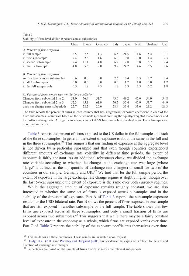
Table 3
Stability of firm-level dollar exposure across subsamples
Chile France Germany Italy Japan Neth Thailand UK
A. Percent of firms exposed
in full sample 3.5 7.5 11.3 6.5 21.5 14.6 15.4 13.1
in first sub-sample 7.4 2.6 1.6 6.6 9.8 13.0 11.4 7.3
in second sub-sample 7.4 11.1 4.8 6.2 17.8 9.8 16.7 17.4
in third sub-sample 4.8 5.3 9.0 9.7 24.2 14.6 15.5 9.6
B. Percent of firms exposed
Across two or more subsamples 0.6 0.0 0.0 2.6 10.4 7.5 3.7 3.4
in all 3 subsamples 0.0 0.0 0.0 0.0 1.2 1.0 0.0 1.7
in the full sample only 0.5 1.8 9.3 1.8 3.3 2.3 6.2 1.8
C. Percent of firms whose sign on the beta coefficient
Changes from subperiod 1 to 2 53.0 56.4 51.7 43.6 49.2 45.0 54.9 54.8
Changes from subperiod 2 to 3 52.3 45.1 61.9 50.7 35.4 45.9 53.7 44.9
does not change acrss subperiods 22.7 28.2 20.0 28.4 35.4 33.0 21.2 26.3
The table reports the percent of firms in each country that has a significant exposure coefficient in each of the
three sub-samples. Results are based on the benchmark specification using the equally-weighted market index and
the dollar exchange rate. All significance levels are set at 5% based on robust standard error. The subsamples are
described in the text.
K.M.E. Dominguez, L.L. Tesar / Journal of International Economics 68 (2006) 188–218 205
Table 3 reports the percent of firms exposed to the US dollar in the full sample and each
of the three subsamples. In general, the extent of exposure is about the same in the full and
in the three subsamples.26 This suggests that our finding of exposure at the aggregate level
is not driven by a particular subsample and that even though countries experienced
different amounts of exchange rate volatility in different time periods, the extent of
exposure is fairly constant. As an additional robustness check, we divided the exchange
rate variable according to whether the change in the exchange rate was large (where
blargeQ is defined as the top quartile of exchange rate changes) or small for two of the
countries in our sample, Germany and UK.27 We find that for the full sample period the
extent of exposure in the large exchange rate change regime is slightly higher, though over
the last 5-year subsample the extent of exposure is the same over both currency regimes.
While the aggregate amount of exposure remains roughly constant, we are also
interested in whether the same set of firms is exposed across subsamples and in the
stability of the direction of exposure. Part A of Table 3 reports the subsample exposure
results for the USD bilateral rate. Part B shows the percent of firms exposed in one sample
that are still exposed in another subsample or the full sample. The table shows that few
firms are exposed across all three subsamples, and only a small fraction of firms are
exposed across two subsamples.28 This suggests that while there may be a fairly constant
level of exposure in the economy as a whole, which firms are exposed varies over time.
Part C of Table 3 reports the stability of the exposure coefficients themselves over time.
26 This holds for all three currencies. These results are available upon request.27 Doidge et al. (2003) and Priestley and Odegaard (2003) find evidence that exposure is related to the size and
direction of exchange rate changes.28 Percentages are based on the sample of firms that exist across the relevant sub-periods.

K.M.E. Dominguez, L.L. Tesar / Journal of International Economics 68 (2006) 188–218206
In 20–35% of the firms that exist over all the subperiods, the sign on the exposure
coefficient stays the same across the three subsamples. And, in about half of the sample
of firms that exist in at least two subperiods, the exposure coefficient switches sign
across at least one subsample, suggesting that both the incidence of exposure (i.e. who is
exposed) and the direction of exposure is time-varying.
The most likely explanation for the time-variation in exposure across the sample is that
it reflects the adaptability of firms to exchange rate risk. Firms that find themselves highly
exposed in one period will react by changing operational or financial policies to offset (or
exploit) any adverse (positive) consequences of the exposure.29 Unfortunately, the detailed
firm-specific time series data necessary to confirm this conjecture is not available for the
wide cross-section of firms included in this study. However, there do exist firm- and
industry-level data that may help us distinguish which firms are most likely to find
themselves exposed to foreign exchange risk. In the next section of the paper we attempt to
explain the average level of firm exposure to exchange rate movements using these data.
5. Explaining exposure: second-stage regressions
In this section we attempt to link the foreign exchange exposure estimates we have
documented in the previous section to firm- and industry-specific characteristics. We test a
series of hypotheses by running a second-stage regression that takes the estimated
exposure betas from Eq. (1) and regresses these on a variety of potential explanatory
variables.
b2;i ¼ k0 þ c1Xi þ ei: ð2Þ
The basic regression specification has the firm-level weekly dollar exposure beta
estimated over the 1994–1999 period as the dependent variable and firm- and industry-
level information as explanatory variables.
Hypothesis 1. Firm-level dollar exposure and firm characteristics.
Our first testable hypothesis is that dollar exposure is a function of firm characteristics,
namely a firm’s size and its industry affiliation. Our prior about the relationship between
firm size and exposure is ambiguous. On the one hand, large firms may be more likely to
be engaged in international activities, and therefore more likely to be affected by exchange
rate movements. On the other hand, larger firms may be more likely to hedge exchange
rate risk, so that smaller firms may be more likely to be exposed.30 To capture firm size,
we sort each country’s sample of firms into thirds based on firm-level market
capitalization. Separate dummies are used for large-sized (top-third) and medium-sized
(middle-third) firms (small-sized firms being the excluded category). We also examine
whether a firm’s industry affiliation is linked to exposure. Datastream provides a set of (2-
29 Allayannis and Ihrig (2001) also find in their study of US industries that exchange rate exposure varies both
over time and switches sign. They hypothesize that these changes in industry exposure are linked to changes in
imported input share, export share and the value of markup.30 Nance et al. (1993) suggest that larger firms are more likely to hedge exchange rate risks.

K.M.E. Dominguez, L.L. Tesar / Journal of International Economics 68 (2006) 188–218 207
digit) industry groupings (10 categories, see the Appendix for a detailed breakdown), from
which we create a set of dummy variables (the excluded category being industry 50
bretailers, restaurants, transportQ).31
The results from the second-stage regressions for each of the eight countries in our
sample are reported in part A of Table 4. The black cells indicate a significant
negative coefficient at the 5% level (based on robust standard errors) and the grey
cells indicate a significant positive coefficient at the 5% level (based on robust
standard errors). The first thing to note from the table is that firm size is generally not
systematically related to exposure betas. It is also striking that most of the significant
industry coefficients are found for Japan.32 Looking over all eight countries, the results
suggest that neither firm size nor industry affiliation consistently explain the variation in
firm level exposure.33
The specification of Eq. (2) is somewhat restricted, however, in that it asks not
only whether firm size and industry play a role in foreign exchange exposure, but it also
implicitly restricts the direction of the exposure to be the same within each of those
categories. It is possible, for example, that two firms in the same industry are strongly
affected by exchange rate movements, but one firm benefits from an exchange rate
appreciation while another firm is made worse off by an appreciation. To test whether our
firm-level explanatory variables contain information about the magnitude of exposure, if
not the direction of the exposure, we next regress the square-root of the absolute value of
the exposure betas on the same set of firm and industry characteristics.34 The results are
reported in Part B of Table 4. The number of significant coefficients on the firm size
dummy variables rises substantially when we ignore the sign on the exposure betas. Now
firm size is statistically significant for six of the eight countries and the sign on the
coefficients suggests that large- and medium-sized firms are likely to have lower levels of
exposure than the excluded category, small firms.35 It is also now the case that the
31 We also tried using a more disaggregated set of industry groupings (at the 4-digit level) in our basic second
stage regression specification. These results, reported in Dominguez and Tesar (2001b), are qualitatively the same
as those reported here using 2-digit industry categories.32 Chamberlain et al. (1997) find that while the returns on US banks are sensitive to exchange rate changes,
Japanese bank returns are not exposed. In Table 4 we find evidence that firms in the Japanese finance industry
(which includes banking, insurance and real estate) are likely to have higher levels of exposure than are firms in
our excluded category (Distributors, Retail, Hotel, Rest and Transport).33 We also experimented with interaction effects between firm size and industry affiliation but found little
evidence that such interactions are operative in the data.34 A number of studies in the literature estimate the second-stage regression using the simple absolute value of
the exposure beta as the dependent variable. This imposes a truncated bias. We include the square root of the
absolute value of the exposure beta, which allows for both positive and negative values and therefore (largely)
leaves the error term normally distributed. It is still the case, however, that this specification restricts the error term
from taking on extremely large negative values. An alternative transformation of the betas, used in Dominguez
and Tesar (2001b), which takes the log odds of the absolute value of beta, is undefined for values of beta that
exceed (�1,1). Our results are qualitatively similar using the two possible transformations of the exposure betas.35 It is worth noting that if derivatives are used by larger firms to hedge exposures, we should expect a negative
relationship between large firms (derivative use) and positive exposure and a positive relationship between large
firms and negative exposures. It is unfortunately not possible to test this hypothesis directly due to the problem of
truncation bias (described in footnote 34).

K.M.E. Dominguez, L.L. Tesar / Journal of International Economics 68 (2006) 188–218208
significant industry coefficients are more evenly distributed across the eight countries.
However, it remains true that the signs on the industry dummies are generally not
consistent across countries. For example, in Germany, Italy and the Netherlands firms in
the Mining, Oil and Gas industry are less exposed than other firms, while the reverse is
true in Japan and the UK. The one industry in which firms across all the countries seem to
be exposed in the same way is the electric, gas and water industry, where the results
suggest that firms in this industry are less exposed than other firms.
Hypothesis 2. Firm-level dollar exposure and international activity.
The second hypothesis we test is whether a firm’s activities in international markets
increase the likelihood of exchange rate exposure.36 We conjecture that the profitability of
multinational firms, and/or firms with significant foreign sales or international assets, will
increase with a depreciation of their home currency relative to the dollar, yielding a
positive coefficient in the first-stage regressions. Those betas, then, will be positively
linked with multinational status. As measures of international activity we include (i) a
dummy variable denoting whether the firm is a multinational corporation, (ii) the firm’s
percentage of foreign to total sales, and (iii) the firm’s percentage of international to total
assets. As described earlier in the paper, firm level data on foreign sales and foreign assets
is limited for most countries, so that the degrees of freedom in these regression
specifications are often quite low. Further, we would expect that firms that are designated
as multinational are also likely to have high levels of foreign assets and foreign sales, so
that the explanatory power of the three variables included in this table should be
qualitatively similar.37
Notes to Table 4:
The table reports the significance of the coefficient on the dummy variable for firm size or industry affiliation in
the following regression
b2i ¼ k0 þ c1Xi þ ei
In part A the dependent variable is the weekly dollar exposure coefficients estimated using Eq. (1) for the 1994–
1999 period.
In part B the regression is repeated using exposure coefficients that are transformed by taking the absolute value
of the square root of the exposure betas.
denotes a significantly positive coefficient at the 5% level based on robust standard errors.
denotes a significantly negative coefficient at the 5% level based on robust standard errors.
denotes a statistically insignificant coefficient at the 5% level based on robust standard errors.
(1) Reference industry for creating firm-size dummies is small, defined as the bottom one-third of the distribution
of the market capitalizations.
(2) Reference industry for creating industry dummies is Distrib, Retail, Hotel, Rest, Transport.
(3) Transformed beta is the square root of the absolute value of the exposure beta.
36 A number of studies in the literature (for example, Jorion, 1990; Bartov et al., 1996; Gao, 1996; Bodnar and
Weintrop, 1997; He and Ng, 1998) test for exchange rate exposure in samples of exclusively multinational firms.37 Note that the multinational status variable is a (1,0) dummy variable while the foreign sales and assets
variables are in percentages. We also tried specifications of Eq. (2) that include dummy variables which
distinguish large, medium and small percentages of foreign sales or assets. We find that results generally did not
change depending on how we specify the variables (as dummies or percentages).

Table 4
Firm-level US dollar exposure and firm characteristics
Part A. Dependent variable: exposure beta estimated over 1994–1999
Firm size (1) LargeMedium
Industry (2) Mining, Oil and GasChem, Const, Forestry, SteelAerosp, Indust, Elect, EngAuto, Hhold goods, TextilesBev, Food, health, Pkg, Pharm, TobFood and drug retail, TelecomElect, Gas and WaterFinance, Ins and Real estateInfo technol., Software and comp
Firm size (1) LargeMedium
Industry (2) Mining, Oil and GasChem, Const, Forestry, SteelAerosp, Indust, Elect, EngAuto, Hhold goods, TextilesBev, Food, health, Pkg, Pharm, TobFood and drug retail, TelecomElect, Gas and WaterFinance, Ins and Real estateInfo technol., Software and comp
Part B. Dependent variable: transformed exposure beta estimated over 1994–1999 (3)
Degree of Freedom
Chile France Germany Italy Japan Neth Thailand UK
194 220 201 274 485 210 386 382
K.M
.E.Dominguez,
L.L.Tesa
r/JournalofIntern
atio
nalEconomics
68(2006)188–218
209

K.M.E. Dominguez, L.L. Tesar / Journal of International Economics 68 (2006) 188–218210
The results of these tests are reported in Table 5, where again a black cell indicates
a significant negative coefficient and a grey cell a significant positive coefficient. The
results suggest that there does appear to be a significant relationship between exposure
and international activity, especially for Germany, Japan and the UK. The results also
suggest that the sign of exposure matters: the second-stage coefficients in the top of
the table are all positive, and there is less explanatory power when we use the
transformed beta coefficients. This is consistent with our conjecture that multi-
nationals, more than other firms in the sample, are likely to benefit from a currency
depreciation.
Table 5
Firm-level US dollar exposure and international activities
Chile France Germany Italy Japan Neth Thailand UK
Part A. Dependent variable: exposure beta estimated over 1994–1999
Multinational status(1)
Foreign sales(2)
International assets(3)
Part B. Dependent variable: transformed exposure beta estimated over 1994-1999 (4)
Multinational status(1)
Foreign sales(2)
International assets(3)
The table reports the significance of the coefficient on the dummy variable for each firm’s multinational status, its
foreign sales and its international assets in the following regression:
b2i ¼ k0 þ c1Xi þ ei
In part A the dependent variable is the weekly dollar exposure coefficients estimated using Eq. (1) for the 1994–
1999 period.
In part B the regression is repeated using exposure coefficients that are transformed by taking the absolute value
of the square root of the exposure betas.
denotes a significantly positive coefficient at the 5% level based on robust standard errors.
denotes a significantly negative coefficient at the 5% level based on robust standard errors.
denotes a statistically insignificant coefficient at the 5% level based on robust standard errors.
indicates missing value due to insufficient data.
(1) The degrees of freedom are 221, 202, 275, 486, 211, 383, respectively, for the 6 countries (excluding Chile
and Thailand).
(2) The degrees of freedom are 25, 118, 106, 193, 365, 125, 211, 292, respectively, for the eight countries.
(3) The degrees of freedom are 48, 58, 70, 337, 36, 203, 272, respectively, for the seven countries (excluding
Chile).
(4) Transformed beta is the square root of the absolute value of the exposure beta.

K.M.E. Dominguez, L.L. Tesar / Journal of International Economics 68 (2006) 188–218 211
Hypothesis 3. Firm-level dollar exposure and international trade.
Another plausible hypothesis regarding exchange rate exposure suggests that firms that
are heavily involved in international trade will be more exposed than purely domestic
firms. Table 6 presents the results of four variants of our second stage regression (2) that
include various proxies for firm-level international trade. The first specification includes a
dummy variable that indicates whether the firm is in a traded-goods industry or a non-
traded industry (see Appendix Table A1 for the list of industries included in each
category). There is no evidence that being a btradedQ or a bnontradedQ classified firm is
systematically linked to exposure.
Our second btradeQ specification includes the volume of world trade flows in exports
and imports for each country by industry.38 Note that the hypothesis is that an exporter will
be more likely to benefit from a depreciation (hence a positive coefficient in the second
stage) and an importer will be more likely to be harmed by a depreciation (yielding a
negative coefficient). The results are strongest for importing firms, where we find a
negative relationship between exposure and the industry-level volume of imports for
Germany, Italy and Japan.
Campa and Goldberg (1997) provide another measure of industry-specific trade
orientation for two of our eight countries, Japan and the UK. They provide measures of
export share, import share and imported input shares for a number of manufacturing
industries in 1993. These data provide another proxy for relative levels of trade across
industries. The results for regression (2) using these data, presented in Table 6, suggest that
all three measures of trade shares are statistically significant for Japan. In the case of
Japan, higher export shares are indeed positively related to firm-level dollar exposure betas
in that industry, while higher imports and imported input shares in an industry are
negatively related to firm level exposure in that industry. While these results are more
encouraging for the hypothesis that trade is related to exposure, it is difficult to know
whether the results for Japan would also hold in a broader set of countries, especially given
that the results are insignificant for the UK.
The final hypothesis we examine is whether market concentration is related to
exposure. The conjecture is that firms in less competitive industries are more likely to pass
exchange rate movements through to prices, and therefore profitability will not be affected
by exchange rate changes. We would expect, then that the coefficient on indicators of
competitiveness would be negative in our second stage regressions. We use two measures
to proxy for market concentration—a Herfindahl index and a markup index, both based on
OECD data. We find that this hypothesis only seems to hold for Japan using the mark-up
index. For France and the UK, the Herfindahl index is significant, but positive. One
explanation for this result is that industries with high Herfindahl indices may contain a few
large firms and numerous smaller firms, so that we may be picking up the small firm size
effect again with this indicator.
38 Again, because the trade data are not available for all the Datastream industries, these regressions include the
subsample of firms in the industries covered by the World Trade Flows data. In addition, we include both the
world trade flows as well as the bilateral flows to the US (to correspond with the dollar exposure betas). Results
using the US bilateral flows are qualitatively similar to those using world trade flows.

K.M.E. Dominguez, L.L. Tesar / Journal of International Economics 68 (2006) 188–218212
5.1. Pooled regressions explaining exposure
All of the analysis we have conducted thus far has been on a country-by-country basis. It
may be the case, however, that there is not enough variation within countries to identify the
distinguishing characteristics of exposed firms relative to non-exposed firms. As a final
robustness check, Table 7 shows the results of a pooled cross-country regression of the firm-
level dollar exposure betas on the indicators for a firm’s international activity and market
structure. We also include country fixed effects. Interestingly, we find that our three
indicators of international activity, and industry-level exports and imports again emerge with
significant coefficients. We also find that the Herfindahl index enters significantly andwith a
positive sign. This confirms the results we find in the country-by-country regressions.
6. Conclusions
We use firm- and industry-level stock returns to test for the presence of exchange rate
exposure in eight countries. We find a significant amount of exposure to a range of
different exchange rates. We find that at the country level, the extent of exposure is robust,
although which firms are affected by movements in the exchange rate and the direction of
exposure depends on the specific exchange rate and varies over time. We postulate that
exchange rate exposure may be linked to a number of firm- and industry-level
characteristics. Our second-stage regressions confirm that exposure is more prevalent in
small- (rather than large- or medium-) sized firms and in firms engaged in international
activities (measured by multinational status, holdings of international assets and foreign
sales). We also find weak evidence linking industry-level measures of international trade
and competitiveness to firm-level exposure.
Notes to Table 6:
The table reports the significance of the coefficient on the dummy variable for the firm’s industry measure of
world trade flow, trade shares, Herfindahl index and markup index in the following regression:
b2i ¼ k0 þ c1Xi þ ei
In part A the dependent variable is the weekly dollar exposure coefficients estimated using Eq. (1) for the 1994–
1999 period.
In part B the regression is repeated using exposure coefficients that are transformed by taking the absolute value
of the square root of the exposure betas.
denotes a significantly positive coefficient at the 5% level based on robust standard errors.
denotes a significantly negative coefficient at the 5% level based on robust standard errors.
denotes a statistically insignificant coefficient at the 5% level based on robust standard errors.
indicates missing value due to insufficient data.
(1) Industry dummy set to 1 if firm is in a traded-good industry. Dof are 192, 214, 202, 263, 483, 210, 347 and
382, respectively, for the 8 countries.
(2) Feenstra world trade industry-level volume data. Degrees of freedom are 86, 110, 111, 130, 279, 97, 176, 123,
respectively, for the 8 countries.
(3) Campa Goldberg trade share data. Degrees of freedom are 253 for Japan and 105 for the UK.
(4) Herfindahl index dofs are 105, 108, 295, 130 for France, Germany, Japan, UK. Markup index dof are 89, 83,
93, 225, 41, 94 (excl Chile and Thailand).
(5) Transformed beta is the square root of the absolute value of the exposure beta.

Table 6
Firm-level US dollar exposure and international trade
Part A. Dependent variable: exposure beta estimated over 1994–1999
Chile France Germany Italy Japan Neth Thailand UK
Traded sector (1)
World trade flows (2) ExportImport
Trade shares (3) Export shareImport shareNet input share
Market concentration (4) Herfindahl index markup index
ExportImport
Export shareImport shareNet input share
Herfindahl index markup index
Part B. Dependent variable: transformed exposure beta estimated over 1994–1999 (5)
Traded sector (1)
World trade flows (2)
Trade shares (3)
Market concentration (4)
K.M
.E.Dominguez,
L.L.Tesa
r/JournalofIntern
atio
nalEconomics
68(2006)188–218
213

Table 7
Cross-country regression using firm-level exposure US$ betas
Independent variables Signed exposure beta (1)
1 2 3 4 5 6 7
Constant �0.064* �0.089* �0.095 �0.051 0.074 �0.034 �0.015
Multinational status 0.168**
Foreign sales 0.002**
International assets 0.006**
Herfindahl index 0.001**
Mark-up index �0.088
Exports 0.006**
Imports �0.771**
Country fixed effects(3)
Chile na 0.184 0.283 na na 0.155* 0.152*
Germany 0.025 �0.014 �0.015 0.069 0.035 0.023 0.031
Italy 0.070* 0.016 0.106 na 0.015 0.016 0.047
Japan �0.025 �0.001 �0.004 �0.042 �0.020 �0.079* �0.048
Netherlands 0.137** 0.042 0.189 na 0.161* 0.131* 0.131*
Thailand na 0.070 �0.071 na na �0.133* �0.094
UK �0.018 0.025 �0.021 0.057 0.065 0.037 0.054
Number of observation 1786 1443 1054 643 635 1122 1122
Adjusted R2 0.028 0.032 0.043 0.021 0.006 0.027 0.023
Independent variables Transformed beta (2)
1 2 3 4 5 6 7
Constant 0.471** 0.446** 0.462** 0.446** 0.501** 0.457** 0.447**
Multinational status 0.024
Foreign sales �0.000
International assets 0.001
Herfindahl index 0.001
Mark-up index �0.036
Exports �0.001
Imports 0.179
Country fixed effects(3)
Chile na 0.227* 0.163 na na 0.099** 0.099**
Germany �0.022 �0.126 �0.029 0.018 0.023 0.015 0.014
Italy �0.38 �0.027 �0.026 na �0.026 �0.018 �0.024
Japan 0.005 0.034 0.014 0.038 0.025 0.039 0.032
Netherlands �0.011 �0.003 0.052 na �0.028 0.015 0.015
Thailand na 0.162** 0.138** na na 0.161** 0.152**
UK 0.035 0.031 0.002 0.054 0.079* 0.051 0.047
Number of observation 1786 1443 1054 643 635 1122 1122
Adjusted R2 0.006 0.053 0.038 0.004 0.009 0.038 0.038
The table shows the results from a pooled regression of exposure betas in the eight countries on dummies for each
firm’s multinational status, foreign sales, international assets, industry-level Herfindahl index, industry-level
mark-up index, industry-level exports and imports, and country fixed effects.
(1) Dollar exposure betas are estimated over 1994–1999.
(2) Transformed beta is the square root of the absolute value of the exposure beta.
(3) Reference country for creating country fixed effects is France.
K.M.E. Dominguez, L.L. Tesar / Journal of International Economics 68 (2006) 188–218214
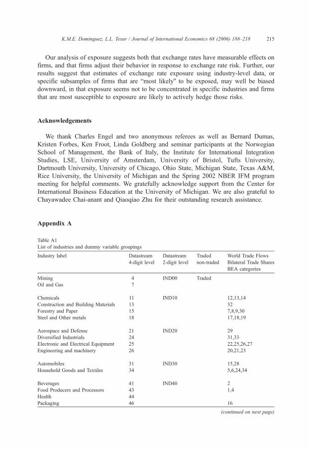
K.M.E. Dominguez, L.L. Tesar / Journal of International Economics 68 (2006) 188–218 215
Our analysis of exposure suggests both that exchange rates have measurable effects on
firms, and that firms adjust their behavior in response to exchange rate risk. Further, our
results suggest that estimates of exchange rate exposure using industry-level data, or
specific subsamples of firms that are bmost likelyQ to be exposed, may well be biased
downward, in that exposure seems not to be concentrated in specific industries and firms
that are most susceptible to exposure are likely to actively hedge those risks.
Acknowledgements
We thank Charles Engel and two anonymous referees as well as Bernard Dumas,
Kristen Forbes, Ken Froot, Linda Goldberg and seminar participants at the Norwegian
School of Management, the Bank of Italy, the Institute for International Integration
Studies, LSE, University of Amsterdam, University of Bristol, Tufts University,
Dartmouth University, University of Chicago, Ohio State, Michigan State, Texas A&M,
Rice University, the University of Michigan and the Spring 2002 NBER IFM program
meeting for helpful comments. We gratefully acknowledge support from the Center for
International Business Education at the University of Michigan. We are also grateful to
Chayawadee Chai-anant and Qiaoqiao Zhu for their outstanding research assistance.
Appendix A
Table A1
List of industries and dummy variable groupings
Industry label Datastream
4-digit level
Datastream
2-digit level
Traded
non-traded
World Trade Flows
Bilateral Trade Shares
BEA categories
Mining 4 IND00 Traded
Oil and Gas 7
Chemicals 11 IND10 12,13,14
Construction and Building Materials 13 32
Forestry and Paper 15 7,8,9,30
Steel and Other metals 18 17,18,19
Aerospace and Defense 21 IND20 29
Diversified Industrials 24 31,33
Electronic and Electrical Equipment 25 22,25,26,27
Engineering and machinery 26 20,21,23
Automobiles 31 IND30 15,28
Household Goods and Textiles 34 5,6,24,34
Beverages 41 IND40 2
Food Producers and Processors 43 1,4
Health 44
Packaging 46 16
(continued on next page)

Table A1 (continued)
Industry Label Datastream
4-digit level
Datastream
2-digit level
Traded
non-traded
World Trade Flows
Bilateral Trade Shares
BEA categories
Personal Care and Household Products 47 11
Pharmaceuticals 48 10
Tobacco 49 3
Distributors 51 IND50 non-traded
Retailers, General 52
Leisure, Entertainment and Hotel 53
Media and Photography 54
Restaurants, Pubs, Breweries 56
Support Services 58
Transport 59
Food and Drug Retailers 63 IND60
Telecom Services 67
Electricity 72 IND70
Gas 73
Water 78
Banks 81 IND80
Insurance 83
Life Assurance 84
Investment companies 85
Real Estate 86
Specialty and other Finance 87
Information Technology Hardware 93 IND90
Software and Computer Services 97
K.M.E. Dominguez, L.L. Tesar / Journal of International Economics 68 (2006) 188–218216
References
Adler, M., Dumas, B., 1984. Exposure to currency risk: definition and measurement. Financial Management 13,
41–50.
Allayannis, G., 1997. The time-variation of the exchange rate exposure: an industry analysis DSWP 97-29,
December.
Allayannis, G., Ihrig, J., 2000. The effect of markups on the exchange rate exposure of stock returns. International
Finance Discussion Papers, vol. 661. Board of Governors of the Federal Reserve System.
Allayannis, G., Ihrig, J., 2001. Exposure and markups. Review of Financial Studies 14 (3), 805–835.
Allayannis, G., Brown, G., Klapper, L., 2003. Capital structure and financial risk: evidence from foreign debt use
in East Asia. Journal of Finance 58 (6), 2667–2710.
Amihud, Y., 1994. Evidence on exchange rates and valuation of equity shares. In: Amihud, Y., Levich, R. (Eds.),
Exchange Rates and Corporate Performance. Irwin Professional Publishing, New York, pp. 49–59.
Bartov, E., Bodnar, G., 1994. Firm valuation, earnings expectations, and the exchange rate exposure effect.
Journal of Finance 49, 1755–1785.
Bartov, E., Bodnar, G., Kaul, A., 1996. Exchange rate variability and the riskiness of U.S. multinational firms:
evidence from the breakdown of the Bretton Woods system. Journal of Financial Economics 42, 105–132.
Bodnar, G., Gentry, W., 1993. Exchange-rate exposure and industry characteristics: evidence from Canada, Japan
and US. Journal of International Money and Finance 12 (1), 29–45.

K.M.E. Dominguez, L.L. Tesar / Journal of International Economics 68 (2006) 188–218 217
Bodnar, G., Marston, R., 2001. A simple model of foreign exchange exposure. In: Negishi, T., Ramachandran,
R., Mino, K. (Eds.), Economic Theory, Dynamics and Markets: Essays in Honor of Ryuzo Sata. Kluwer,
New York.
Bodnar, G., Weintrop, J., 1997. The valuation of the foreign income of U.S. multinational firms: a growth
opportunities perspective. Journal of Accounting and Economics 24, 69–97.
Bodnar, G., Wong, F., 2003. Estimating exchange rate exposures: issues in model structure. Financial
Management 32 (1), 35–67.
Bodnar, G., Hayt, G., Marston, R., 1998. Wharton 1998 survey of risk management by US non-financial firms.
Financial Management 27, 4.
Bodnar, G., Dumas, B., Marston, R., 2002. Pass-through and exposure. Journal of Finance 57 (1), 199–231.
Campa, J., Goldberg, L., 1995. Investment in manufacturing, exchange-rates and external exposure. Journal of
International Economics 38, 297–320.
Campa, J., Goldberg, L., 1997. The evolving external orientation of manufacturing: a profile of four countries.
FRBNY Economic Policy, 53–81.
Campa, J., Goldberg, L., 1999. Investment, pass-through and exchange rates: a cross-country comparison.
International Economic Review 40 (2), 287–314.
Chamberlain, S., Howe, J., Popper, H., 1997. The exchange rate exposure of U.S. and Japanese banking
institutions. Journal of Banking and Finance 21, 871–892.
Chow, E., Lee, W., Solt, M., 1997a. The exchange rate exposure of asset returns. Journal of Business 70 (1),
105–123.
Chow, E., Lee, W., Solt, M., 1997b. The economic exposure of U.S. multinational firms. The Journal of Financial
Research, 191–210.
Connolly, R.A., Ozoguz, A., Ravenscraft, D.J., 2000. Foreign market cash flow exposure: a multi-country, firm-
level study. University of North Carolina Working Paper.
Dekle, R., 2000. Exchange rates and corporate exposure: evidence from Japanese firm level panel data. USC
Working Paper, April.
Doidge, C., Griffin, J., Williamson, R., 2003. The international determinants and the economic importance of
exchange rate exposure. Mimeo, June.
Dominguez, K., 1998. The dollar exposure of Japanese companies. Journal of Japanese and International
Economics 12, 388–405.
Dominguez, K., Tesar, L., 2001a. A re-examination of exchange rate exposure. American Economic Review
Papers and Proceedings 91, 2396–2399.
Dominguez, K., Tesar, L., 2001b. Trade and exposure. American Economic Review Papers and Proceedings 91
(2), 367–370.
Feenstra, R., 2000. World trade flows: 1980–1997, March.
Financial Times Multinational Index, 2000.
Forbes, K., 2002. Are trade linkages important determinants of country vulnerability to crises? In: Edwards, S.,
Frankel, J. (Eds.), Currency Crisis Prevention. University of Chicago Press for the NBER, pp. 77–128.
Frankel, J., Rose, A., 2002. An estimate of the effect of common currencies on trade and income. Quarterly
Journal of Economics, 437–466.
Frennberg, P., 1994. Stock prices and large exchange rate adjustments: some Swedish experience. Journal of
International Financial Markets, Institutions, and Money 4 (3/4), 127–148.
Gao, T., 1996. Exchange rate movements and the profitability of U.S. multinationals. University of Michigan
working paper.
Griffin, J., Stulz, R., 2001. International competition and exchange rate shocks: a cross-country industry analysis
of stock returns. Review of Financial Studies, 215–241.
He, J., Ng, L., 1998. The foreign exchange exposure of japanese multinational corporations. Journal of Finance
LIII (2), 733–753.
Jorion, P., 1990. The exchange rate exposure of U.S. multinationals. Journal of Business 63, 33–45.
Loderer, C., Pichler, K., 2000. Firms, do you know your currency risk exposure?Q Universitat Bern Working
Paper.
Marston, R., 2001. The effects of industry structure on economic exposure. Journal of International Money and
Finance 20, 149–164.

K.M.E. Dominguez, L.L. Tesar / Journal of International Economics 68 (2006) 188–218218
Nance, D., Smith, C., Smithson, C., 1993. On the determinants of corporate hedging. Journal of Finance 1,
267–284.
Nucci, F., Pozzolo, A.F., 2001. Investment and the exchange rate: an analysis with firm-level panel data.
European Economic Review 45, 259–283.
Oliveira Martins, J.O., Scarpetta, S., Pilat, D., 1996. Mark-up ratios in manufacturing industries: estimates for 14
OECD countries. OECD Economics Department WP No. 162.
Priestley, R., Odegaard, B.A., 2003. Long Swings in the Dollar and the Exchange Rate Exposure of Stock
Returns. Norwegian School of Management. (July).
Roeger, W., 1995. Can imperfect competition explain the difference between primal and dual productivity
measures? Estimates for US manufacturing. Journal of Political Economy 103, 316–330.
The Directory of Multinationals, 1998.
Williamson, R., 2001. Exchange rate exposure and competition: evidence from the world automotive industry.
Journal of Financial Economics 59, 441–475.
Worldwide Branch Locations of Multinationals, 1994.