Domain TheoryCorrected and expanded version

Samson Abramsky1 and Achim Jung2

This text is based on the chapter Domain Theory in the Handbook for Logic inComputer Science, volume 3, edited by S. Abramsky, Dov M. Gabbay, and T. S.E. Maibaum, published by Clarendon Press, Oxford in 1994. While the numbering ofall theorems and definitions has been kept the same, we have included comments andcorrections which we have received over the years. For ease of reading, small typo-graphical errors have simply been corrected. Where we felt the original text gave amisleading impression, we have included additional explanations, clearly marked assuch.

If you wish to refer to this text, then please cite the published original version wherepossible, or otherwise this on-line version which we try to keep available from the pagehttp://www.cs.bham.ac.uk/!axj/papers.html

We will be grateful to receive further comments or suggestions. Please send themto A.Jung@cs.bham.ac.uk

So far, we have received comments and/or corrections from Francesco Consentino,Joseph D. Darcy, Mohamed El-Zawawy, Weng Kin Ho, Klaus Keimel, Olaf Klinke,Xuhui Li, Homeira Pajoohesh, Dieter Spreen, and Dominic van der Zypen.

1Computing Laboratory, University of Oxford, Wolfson Building, Parks Road, Oxford, OX1 3QD, Eng-land.

2School of Computer Science, University of Birmingham, Edgbaston, Birmingham, B15 2TT, England.

Contents1 Introduction and Overview 5

1.1 Origins . . . . . . . . . . . . . . . . . . . . . . . . . . . . . . . . . 51.2 Our approach . . . . . . . . . . . . . . . . . . . . . . . . . . . . . . 71.3 Overview . . . . . . . . . . . . . . . . . . . . . . . . . . . . . . . . 7

2 Domains individually 102.1 Convergence . . . . . . . . . . . . . . . . . . . . . . . . . . . . . . 10

2.1.1 Posets and preorders . . . . . . . . . . . . . . . . . . . . . . 102.1.2 Notation from order theory . . . . . . . . . . . . . . . . . . . 112.1.3 Monotone functions . . . . . . . . . . . . . . . . . . . . . . 132.1.4 Directed sets . . . . . . . . . . . . . . . . . . . . . . . . . . 132.1.5 Directed-complete partial orders . . . . . . . . . . . . . . . . 142.1.6 Continuous functions . . . . . . . . . . . . . . . . . . . . . . 15

2.2 Approximation . . . . . . . . . . . . . . . . . . . . . . . . . . . . . 172.2.1 The order of approximation . . . . . . . . . . . . . . . . . . 182.2.2 Bases in dcpo’s . . . . . . . . . . . . . . . . . . . . . . . . . 182.2.3 Continuous and algebraic domains . . . . . . . . . . . . . . . 192.2.4 Comments on possible variations . . . . . . . . . . . . . . . 222.2.5 Useful properties . . . . . . . . . . . . . . . . . . . . . . . . 242.2.6 Bases as objects . . . . . . . . . . . . . . . . . . . . . . . . . 25

2.3 Topology . . . . . . . . . . . . . . . . . . . . . . . . . . . . . . . . 292.3.1 The Scott-topology on a dcpo . . . . . . . . . . . . . . . . . 292.3.2 The Scott-topology on domains . . . . . . . . . . . . . . . . 30

3 Domains collectively 343.1 Comparing domains . . . . . . . . . . . . . . . . . . . . . . . . . . . 34

3.1.1 Retractions . . . . . . . . . . . . . . . . . . . . . . . . . . . 343.1.2 Idempotents . . . . . . . . . . . . . . . . . . . . . . . . . . . 353.1.3 Adjunctions . . . . . . . . . . . . . . . . . . . . . . . . . . . 363.1.4 Projections and sub-domains . . . . . . . . . . . . . . . . . . 393.1.5 Closures and quotient domains . . . . . . . . . . . . . . . . . 40

3.2 Finitary constructions . . . . . . . . . . . . . . . . . . . . . . . . . . 413.2.1 Cartesian product . . . . . . . . . . . . . . . . . . . . . . . . 423.2.2 Function space . . . . . . . . . . . . . . . . . . . . . . . . . 433.2.3 Coalesced sum . . . . . . . . . . . . . . . . . . . . . . . . . 443.2.4 Smash product and strict function space . . . . . . . . . . . . 453.2.5 Lifting . . . . . . . . . . . . . . . . . . . . . . . . . . . . . 453.2.6 Summary . . . . . . . . . . . . . . . . . . . . . . . . . . . . 45

3.3 Infinitary constructions . . . . . . . . . . . . . . . . . . . . . . . . . 463.3.1 Limits and colimits . . . . . . . . . . . . . . . . . . . . . . . 463.3.2 The limit-colimit coincidence . . . . . . . . . . . . . . . . . 473.3.3 Bilimits of domains . . . . . . . . . . . . . . . . . . . . . . . 51

2

4 Cartesian closed categories of domains 544.1 Local uniqueness: Lattice-like domains . . . . . . . . . . . . . . . . 554.2 Finite choice: Compact domains . . . . . . . . . . . . . . . . . . . . 57

4.2.1 Bifinite domains . . . . . . . . . . . . . . . . . . . . . . . . 574.2.2 FS-domains . . . . . . . . . . . . . . . . . . . . . . . . . . . 604.2.3 Coherence . . . . . . . . . . . . . . . . . . . . . . . . . . . 61

4.3 The hierarchy of categories of domains . . . . . . . . . . . . . . . . . 634.3.1 Domains with least element . . . . . . . . . . . . . . . . . . 634.3.2 Domains without least element . . . . . . . . . . . . . . . . . 65

5 Recursive domain equations 685.1 Examples . . . . . . . . . . . . . . . . . . . . . . . . . . . . . . . . 68

5.1.1 Genuine equations . . . . . . . . . . . . . . . . . . . . . . . 685.1.2 Recursive definitions . . . . . . . . . . . . . . . . . . . . . . 685.1.3 Data types . . . . . . . . . . . . . . . . . . . . . . . . . . . . 69

5.2 Construction of solutions . . . . . . . . . . . . . . . . . . . . . . . . 705.2.1 Continuous functors . . . . . . . . . . . . . . . . . . . . . . 705.2.2 Local continuity . . . . . . . . . . . . . . . . . . . . . . . . 715.2.3 Parameterized equations . . . . . . . . . . . . . . . . . . . . 73

5.3 Canonicity . . . . . . . . . . . . . . . . . . . . . . . . . . . . . . . . 745.3.1 Invariance and minimality . . . . . . . . . . . . . . . . . . . 745.3.2 Initiality and finality . . . . . . . . . . . . . . . . . . . . . . 765.3.3 Mixed variance . . . . . . . . . . . . . . . . . . . . . . . . . 77

5.4 Analysis of solutions . . . . . . . . . . . . . . . . . . . . . . . . . . 795.4.1 Structural induction on terms . . . . . . . . . . . . . . . . . . 795.4.2 Admissible relations . . . . . . . . . . . . . . . . . . . . . . 805.4.3 Induction with admissible relations . . . . . . . . . . . . . . 815.4.4 Co-induction with admissible relations . . . . . . . . . . . . 82

6 Equational theories 856.1 General techniques . . . . . . . . . . . . . . . . . . . . . . . . . . . 85

6.1.1 Free dcpo-algebras . . . . . . . . . . . . . . . . . . . . . . . 856.1.2 Free continuous domain-algebras . . . . . . . . . . . . . . . 876.1.3 Least elements and strict algebras . . . . . . . . . . . . . . . 92

6.2 Powerdomains . . . . . . . . . . . . . . . . . . . . . . . . . . . . . . 936.2.1 The convex or Plotkin powerdomain . . . . . . . . . . . . . . 936.2.2 One-sided powerdomains . . . . . . . . . . . . . . . . . . . . 966.2.3 Topological representation theorems . . . . . . . . . . . . . . 976.2.4 Hyperspaces and probabilistic powerdomains . . . . . . . . . 103

7 Domains and logic 1067.1 Stone duality . . . . . . . . . . . . . . . . . . . . . . . . . . . . . . 106

7.1.1 Approximation and distributivity . . . . . . . . . . . . . . . . 1067.1.2 From spaces to lattices . . . . . . . . . . . . . . . . . . . . . 1097.1.3 From lattices to topological spaces . . . . . . . . . . . . . . . 1107.1.4 The basic adjunction . . . . . . . . . . . . . . . . . . . . . . 111

3

7.2 Some equivalences . . . . . . . . . . . . . . . . . . . . . . . . . . . 1127.2.1 Sober spaces and spatial lattices . . . . . . . . . . . . . . . . 1127.2.2 Properties of sober spaces . . . . . . . . . . . . . . . . . . . 1147.2.3 Locally compact spaces and continuous lattices . . . . . . . . 1167.2.4 Coherence . . . . . . . . . . . . . . . . . . . . . . . . . . . 1177.2.5 Compact-open sets and spectral spaces . . . . . . . . . . . . 1177.2.6 Domains . . . . . . . . . . . . . . . . . . . . . . . . . . . . 1197.2.7 Summary . . . . . . . . . . . . . . . . . . . . . . . . . . . . 121

7.3 The logical viewpoint . . . . . . . . . . . . . . . . . . . . . . . . . . 1217.3.1 Working with lattices of compact-open subsets . . . . . . . . 1217.3.2 Constructions: The general technique . . . . . . . . . . . . . 1267.3.3 The function space construction . . . . . . . . . . . . . . . . 1307.3.4 The Plotkin powerlocale . . . . . . . . . . . . . . . . . . . . 1327.3.5 Recursive domain equations . . . . . . . . . . . . . . . . . . 1367.3.6 Languages for types, properties, and points . . . . . . . . . . 137

8 Further directions 1458.1 Further topics in “Classical Domain Theory” . . . . . . . . . . . . . 145

8.1.1 Effectively given domains . . . . . . . . . . . . . . . . . . . 1458.1.2 Universal Domains . . . . . . . . . . . . . . . . . . . . . . . 1458.1.3 Domain-theoretic semantics of polymorphism . . . . . . . . . 1468.1.4 Information Systems . . . . . . . . . . . . . . . . . . . . . . 146

8.2 Stability and Sequentiality . . . . . . . . . . . . . . . . . . . . . . . 1478.3 Reformulations of Domain Theory . . . . . . . . . . . . . . . . . . . 147

8.3.1 Predomains and partial functions . . . . . . . . . . . . . . . . 1488.3.2 Computational Monads . . . . . . . . . . . . . . . . . . . . . 1488.3.3 Linear Types . . . . . . . . . . . . . . . . . . . . . . . . . . 149

8.4 Axiomatic Domain Theory . . . . . . . . . . . . . . . . . . . . . . . 1508.5 Synthetic Domain Theory . . . . . . . . . . . . . . . . . . . . . . . . 151

9 Guide to the literature 152

References 153

Index 165

4

1 Introduction and Overview1.1 OriginsLet us begin with the problems which gave rise to Domain Theory:

1. Least fixpoints as meanings of recursive definitions. Recursive definitions ofprocedures, data structures and other computational entities abound in program-ming languages. Indeed, recursion is the basic effective mechanism for describ-ing infinite computational behaviour in finite terms. Given a recursive definition:

X = . . . X . . . (1)

How can we give a non-circular account of its meaning? Suppose we are work-ing inside some mathematical structure D. We want to find an element d ! Dsuch that substituting d for x in (1) yields a valid equation. The right-hand-sideof (1) can be read as a function of X , semantically as f : D " D. We can nowsee that we are asking for an element d ! D such that d = f(d)—that is, for afixpoint of f . Moreover, we want a uniform canonical method for constructingsuch fixpoints for arbitrary structures D and functions f : D " D within ourframework. Elementary considerations show that the usual categories of math-ematical structures either fail to meet this requirement at all (sets, topologicalspaces) or meet it in a trivial fashion (groups, vector spaces).

2. Recursive domain equations. Apart from recursive definitions of computa-tional objects, programming languages also abound, explicitly or implicitly, inrecursive definitions of datatypes. The classical example is the type-free !-calculus [Bar84]. To give a mathematical semantics for the !-calculus is to finda mathematical structure D such that terms of the !-calculus can be interpretedas elements of D in such a way that application in the calculus is interpretedby function application. Now consider the self-application term !x.xx. By theusual condition for type-compatibility of a function with its argument, we seethat if the second occurrence of x in xx has type D, and the whole term xx hastype D, then the first occurrence must have, or be construable as having, type[D #" D]. Thus we are led to the requirement that we have

[D #" D] $= D.

If we view [. #" .] as a functor F : Cop % C " C over a suitable category Cof mathematical structures, then we are looking for a fixpoint D $= F (D, D).Thus recursive datatypes again lead to a requirement for fixpoints, but now liftedto the functorial level. Again we want such fixpoints to exist uniformly andcanonically.

This second requirement is even further beyond the realms of ordinary mathemati-cal experience than the first. Collectively, they call for a novel mathematical theory toserve as a foundation for the semantics of programming languages.

5

A first step towards Domain Theory is the familiar result that every monotonefunction on a complete lattice, or more generally on a directed-complete partial or-der with least element, has a least fixpoint. (For an account of the history of thisresult, see [LNS82].) Some early uses of this result in the context of formal lan-guage theory were [Ard60, GR62]. It had also found applications in recursion theory[Kle52, Pla64]. Its application to the semantics of first-order recursion equations andflowcharts was already well-established among Computer Scientists by the end of the1960’s [dBS69, Bek69, Bek71, Par69]. But Domain Theory proper, at least as we un-derstand the term, began in 1969, and was unambiguously the creation of one man,Dana Scott [Sco69, Sco70, Sco71, Sco72, Sco93]. In particular, the following keyinsights can be identified in his work:

1. Domains as types. The fact that suitable categories of domains are cartesianclosed, and hence give rise to models of typed !-calculi. More generally, thatdomains give mathematical meaning to a broad class of data-structuring mecha-nisms.

2. Recursive types. Scott’s key construction was a solution to the “domain equa-tion”

D $= [D #" D]

thus giving the first mathematical model of the type-free !-calculus. This ledto a general theory of solutions of recursive domain equations. In conjunctionwith (1), this showed that domains form a suitable universe for the semantics ofprogramming languages. In this way, Scott provided a mathematical foundationfor the work of Christopher Strachey on denotational semantics [MS76, Sto77].This combination of descriptive richness and a powerful and elegant mathemati-cal theory led to denotational semantics becoming a dominant paradigm in The-oretical Computer Science.

3. Continuity vs. Computability. Continuity is a central pillar of Domain theory.It serves as a qualitative approximation to computability. In other words, formost purposes to detect whether some construction is computationally feasibleit is sufficient to check that it is continuous; while continuity is an “algebraic”condition, which is much easier to handle than computability. In order to givethis idea of continuity as a smoothed-out version of computability substance, itis not sufficient to work only with a notion of “completeness” or “convergence”;one also needs a notion of approximation, which does justice to the idea thatinfinite objects are given in some coherent way as limits of their finite approx-imations. This leads to considering, not arbitrary complete partial orders, butthe continuous ones. Indeed, Scott’s early work on Domain Theory was semi-nal to the subsequent extensive development of the theory of continuous lattices,which also drew heavily on ideas from topology, analysis, topological algebraand category theory [GHK+80].

4. Partial information. A natural concomitant of the notion of approximation indomains is that they form the basis of a theory of partial information, which ex-tends the familiar notion of partial function to encompass a whole spectrum of

6

“degrees of definedness”. This has important applications to the semantics ofprogramming languages, where such multiple degrees of definition play a keyrole in the analysis of computational notions such as lazy vs. eager evaluation,and call-by-name vs. call-by-value parameter-passing mechanisms for proce-dures.General considerations from recursion theory dictate that partial functions areunavoidable in any discussion of computability. Domain Theory provides anappropriately abstract, structural setting in which these notions can be lifted tohigher types, recursive types, etc.

1.2 Our approachIt is a striking fact that, although Domain Theory has been around for a quarter-century, no book-length treatment of it has yet been published. Quite a number ofbooks on semantics of programming languages, incorporating substantial introduc-tions to domain theory as a necessary tool for denotational semantics, have appeared[Sto77, Sch86, Gun92b, Win93]; but there has been no text devoted to the underlyingmathematical theory of domains. To make an analogy, it is as if many Calculus text-books were available, offering presentations of some basic analysis interleaved with itsapplications in modelling physical and geometrical problems; but no textbook of RealAnalysis. Although this Handbook Chapter cannot offer the comprehensive coverageof a full-length textbook, it is nevertheless written in the spirit of a presentation of RealAnalysis. That is, we attempt to give a crisp, efficient presentation of the mathematicaltheory of domains without excursions into applications. We hope that such an accountwill be found useful by readers wishing to acquire some familiarity with Domain The-ory, including those who seek to apply it. Indeed, we believe that the chances forexciting new applications of Domain Theory will be enhanced if more people becomeaware of the full richness of the mathematical theory.

1.3 OverviewDomains individually

We begin by developing the basic mathematical language of Domain Theory, and thenpresent the central pillars of the theory: convergence and approximation. We put con-siderable emphasis on bases of continuous domains, and show how the theory can bedeveloped in terms of these. We also give a first presentation of the topological viewof Domain Theory, which will be a recurring theme.

Domains collectively

We study special classes of maps which play a key role in domain theory: retractions,adjunctions, embeddings and projections. We also look at construction on domainssuch as products, function spaces, sums and lifting; and at bilimits of directed systemsof domains and embeddings.

7

Cartesian closed categories of domains

A particularly important requirement on categories of domains is that they should becartesian closed (i.e. closed under function spaces). This creates a tension with therequirement for a good theory of approximation for domains, since neither the categoryCONT of all continuous domains, nor the category ALG of all algebraic domainsis cartesian closed. This leads to a non-trivial analysis of necessary and sufficientconditions on domains to ensure closure under function spaces, and striking resultson the classification of the maximal cartesian closed full subcategories of CONT andALG. This material is based on [Jun89, Jun90].

Recursive domain equations

The theory of recursive domain equations is presented. Although this material formedthe very starting point of Domain Theory, a full clarification of just what canonicity ofsolutions means, and how it can be translated into proof principles for reasoning aboutthese canonical solutions, has only emerged over the past two or three years, throughthe work of Peter Freyd and Andrew Pitts [Fre91, Fre92, Pit93b]. We make extensiveuse of their insights in our presentation.

Equational theories

We present a general theory of the construction of free algebras for inequational theo-ries over continuous domains. These results, and the underlying constructions in termsof bases, appear to be new. We then apply this general theory to powerdomains andgive a comprehensive treatment of the Plotkin, Hoare and Smyth powerdomains. In ad-dition to characterizing these as free algebras for certain inequational theories, we alsoprove representation theorems which characterize a powerdomain over D as a certainspace of subsets ofD; these results make considerable use of topological methods.

Domains and logic

We develop the logical point of view of Domain Theory, in which domains are charac-terized in terms of their observable properties, and functions in terms of their actionson these properties. The general framework for this is provided by Stone duality; wedevelop the rudiments of Stone duality in some generality, and then specialize it todomains. Finally, we present “Domain Theory in Logical Form” [Abr91b], in which ametalanguage of types and terms suitable for denotational semantics is extended witha language of properties, and presented axiomatically as a programming logic in sucha way that the lattice of properties over each type is the Stone dual of the domain de-noted by that type, and the prime filter of properties which can be proved to hold ofa term correspond under Stone duality to the domain element denoted by that term.This yields a systematic way of moving back and forth between the logical and deno-tational descriptions of some computational situation, each determining the other up toisomorphism.

8

AcknowledgementsWe would like to thank Jirı Adamek, Reinhold Heckmann, Michael Huth, MathiasKegelmann, Philipp Sunderhauf, and Paul Taylor for very careful proof reading. AchimJung would particularly like to thank the people from the “Domain Theory Group” atDarmstadt, who provided a stimulating and supportive environment.

Our major intellectual debts, inevitably, are to Dana Scott and Gordon Plotkin. Themore we learn about Domain Theory, the more we appreciate the depth of their insights.

9

2 Domains individuallyWe will begin by introducing the basic language of Domain Theory. Most topics wedeal with in this section are treated more thoroughly and at a more leisurely pace in[DP90].

2.1 Convergence2.1.1 Posets and preorders

Definition 2.1.1. A set P with a binary relation & is called a partially ordered set orposet if the following holds for all x, y, z ! P :

1. x & x (Reflexivity)

2. x & y ' y & z =( x & z (Transitivity)

3. x & y ' y & x =( x = y (Antisymmetry)

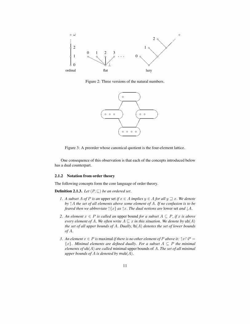
Small finite partially ordered sets can be drawn as line diagrams (Hasse diagrams).Examples are given in Figure 1. We will also allow ourselves to draw infinite posetsby showing a finite part which illustrates the building principle. Three examples aregiven in Figure 2. We prefer the notation & to the more common ) because the orderon domains we are studying here often coexists with an otherwise unrelated intrinsicorder. The flat and lazy natural numbers from Figure 2 illustrate this.

If we drop antisymmetry from our list of requirements then we get what is knownas preorders. This does not change the theory very much. As is easily seen, the sub-relation & * + is in any case an equivalence relation and if two elements from twoequivalence classes x ! A, y ! B are related by &, then so is any pair of elementsfrom A and B. We can therefore pass from a preorder to a canonical partially orderedset by taking equivalence classes. Pictorially, the situation then looks as in Figure 3.

Many notions from the theory of ordered sets make sense even if reflexivity fails.Hence we may sum up these considerations with the slogan: Order theory is the studyof transitive relations. A common way to extract the order-theoretic content from arelation R is to pass to the transitive closure of R, defined as

!

n"N\{0} Rn.Ordered sets can be turned upside down:

Proposition 2.1.2. If ,P,&- is an ordered set then so is P op = ,P,+-.

!The flat booleans

.

!true !false

!! "

" !The four-element lattice

! !!

!!"

" !!"

" !The four-element chain

!!!

Figure 1: A few posets drawn as line diagrams.

10

!ordinal

0

! 1! 2

! """"

!flat

.

!0 !1 !2 !3 " " "####!!

"" !

lazy

!0 !!1 !

!2!

" " "

!! "

""

"""

!!

!!

Figure 2: Three versions of the natural numbers.

! ! ! !

! ! ! ! !

!

$$$

%%%

%%%

$$$

#$

%&

#$

%&

#$

%&

#$

%&

Figure 3: A preorder whose canonical quotient is the four-element lattice.

One consequence of this observation is that each of the concepts introduced belowhas a dual counterpart.

2.1.2 Notation from order theory

The following concepts form the core language of order theory.

Definition 2.1.3. Let (P,&) be an ordered set.

1. A subset A of P is an upper set if x ! A implies y ! A for all y + x. We denoteby /A the set of all elements above some element of A. If no confusion is to befeared then we abbreviate /{x} as /x. The dual notions are lower set and 0A.

2. An element x ! P is called an upper bound for a subset A 1 P , if x is aboveevery element of A. We often write A & x in this situation. We denote by ub(A)the set of all upper bounds of A. Dually, lb(A) denotes the set of lower boundsof A.

3. An element x ! P ismaximal if there is no other element of P above it: /x*P ={x}. Minimal elements are defined dually. For a subset A 1 P the minimalelements of ub(A) are called minimal upper bounds of A. The set of all minimalupper bounds of A is denoted by mub(A).

11

4. If all elements of P are below a single element x ! P , then x is said to be thelargest element. The dually defined least element of a poset is also called bottomand is commonly denoted by .. In the presence of a least element we speak of apointed poset.

5. If for a subset A 1 P the set of upper bounds has a least element x, then xis called the supremum or join. We write x =

"

A in this case. In the otherdirection we speak of infimum or meet and write x =

!A.

6. A partially ordered set P is a 2-semilattice (3-semilattice) if the supremum (in-fimum) for each pair of elements exists. If P is both a 2- and a 3-semilatticethen P is called a lattice. A lattice is complete if suprema and infima exist for allsubsets.

The operations of forming suprema, resp. infima, have a few basic properties whichwe will use throughout this text without mentioning them further.

Proposition 2.1.4. Let P be a poset such that the suprema and infima occurring in thefollowing formulae exist. (A, B and all Ai are subsets of P .)

1. A 1 B implies"

A &"

B and!

A +!

B.

2."

A ="

(0A) and!

A =!

(/A).

3. If A =!

i"I Ai then"

A ="

i"I("

Ai) and similarly for the infimum.

Proof. We illustrate order theoretic reasoning with suprema by showing (3). The el-ement

"

A is above each element"

Ai by (1), so it is an upper bound of the set{"

Ai | i ! I}. Since"

i"I("

Ai) is the least upper bound of this set, we have"

A +"

i"I("

Ai). Conversely, each a ! A is contained in some Ai and there-fore below the corresponding

"

Ai which in turn is below"

i"I("

Ai). Hence theright hand side is an upper bound of A and as

"

A is the least such, we also have"

A &"

i"I("

Ai).

Let us conclude this subsection by looking at an important family of examples ofcomplete lattices. Suppose X is a set and L is a family of subsets of X . We callL a closure system if it is closed under the formation of intersections, that is, when-ever each member of a family (Ai)i"I belongs to L then so does

#

i"I Ai. Becausewe have allowed the index set to be empty, this implies that X is in L. We call themembers of L hulls or closed sets. Given an arbitrary subset A of X , one can form#

{B ! L | A 1 B}. This is the least superset of A which belongs to L and is calledthe hull or the closure of A.

Proposition 2.1.5. Every closure system is a complete lattice with respect to inclusion.

Proof. Infima are given by intersections and for the supremum one takes the closure ofthe union.

12

2.1.3 Monotone functions

Definition 2.1.6. Let P and Q be partially ordered sets. A function f : P " Q iscalled monotone if for all x, y ! P with x & y we also have f(x) & f(y) in Q.

‘Monotone’ is really an abbreviation for ‘monotone order-preserving’, but since wehave no use for monotone order-reversing maps (x & y =( f(x) + f(y)), we haveopted for the shorter expression. Alternative terminology is isotone (vs. antitone) orthe other half of the full expression: order-preservingmapping.

The set [Pm#" Q] of all monotone functions between two posets, when ordered

pointwise (i.e. f & g if for all x ! P , f(x) & g(x)), gives rise to another partiallyordered set, the monotone function space between P and Q. The category POSET ofposets and monotone maps has pleasing properties, see Exercise 2.3.9(9).

Proposition 2.1.7. If L is a complete lattice then every monotone map from L to L hasa fixpoint. The least of these is given by

"{x ! L | f(x) & x} ,

the largest by$

{x ! L | x & f(x)} .

Proof. Let A = {x ! L | f(x) & x} and a =!

A. For each x ! A we have a & xand f(a) & f(x) & x. Taking the infimum we get f(a) &

!f(A) &

!A = a and

a ! A follows. On the other hand, x ! A always implies f(x) ! A by monotonicity.Applying this to a yields f(a) ! A and hence a & f(a).

For lattices, the converse is also true: The existence of fixpoints for monotonemapsimplies completeness. But the proof is much harder and relies on the Axiom of Choice,see [Mar76].

2.1.4 Directed sets

Definition 2.1.8. Let P be a poset. A subset A of P is directed, if it is nonempty andeach pair of elements ofA has an upper bound inA. If a directed setA has a supremumthen this is denoted by

"

#A.Directed lower sets are called ideals. Ideals of the form 0x are called principal.The dual notions are filtered set and (principal) filter.

Simple examples of directed sets are chains. These are non-empty subsets whichare totally ordered, i.e. for each pair x, y either x & y or y & x holds. The chainof natural numbers with their natural order is particularly simple; subsets of a posetisomorphic to it are usually called "-chains. Another frequent type of directed set isgiven by the set of finite subsets of an arbitrary set. Using this and Proposition 2.1.4(3),we get the following useful decomposition of general suprema.

Proposition 2.1.9. Let A be a non-empty subset of a 2-semilattice for which"

Aexists. Then the join of A can also be written as

$

#{$

M | M 1 A finite and non-empty} .

13

General directed sets, on the other hand, may be quite messy and unstructured.Sometimes one can find a well-behaved cofinal subset, such as a chain, where we saythat A is cofinal in B, if for all b ! B there is an a ! A above it. Such a cofinal subsetwill have the same supremum (if it exists). But cofinal chains do not always exist, asExercise 2.3.9(6) shows. Still, every directed set may be thought of as being equippedexternally with a nice structure as we will now work out.

Definition 2.1.10. A monotone net in a poset P is a monotone function # from adirected set I into P . The set I is called the index set of the net.

Let # : I " P be a monotone net. If we are given a monotone function $ : J " I ,where J is directed and where for all i ! I there is j ! J with $(j) 4 i, then we call# 5 $ : J " P a subnet of #.

A monotone net # : I " P has a supremum in P , if the set {#(i) | i ! I} has asupremum in P .

Every directed set can be viewed as a monotone net: let the set itself be the indexset. On the other hand, the image of a monotone net # : I " P is a directed set in P .So what are nets good for? The answer is given in the following proposition (whichseems to have been stated first in [Kra39]).

Lemma 2.1.11. Let P be a poset and let # : I " P be a monotone net. Then # has asubnet # 5 $ : J " P , whose index set J is a lattice in which every principal ideal isfinite.

Proof. Let J be the set of finite subsets of I . Clearly, J is a lattice in which every prin-cipal ideal is finite. We define the mapping $ : J " I by induction on the cardinalityof the elements of J :

$(%) = any element of I;

$(A) = any upper bound of the set A 6 {$(B) | B 7 A}, A 8= %.

It is obvious that $ is monotone and defines a subnet.

This lemma allows us to base an induction proof on an arbitrary directed set. Thiswas recently applied to settle a long-standing conjecture in lattice theory, see [TT93].

Proposition 2.1.12. Let I be directed and # : I % I " P be a monotone net. Underthe assumption that the indicated directed suprema exist, the following equalities hold:

$

#

i,j"I

#(i, j) =$

#

i"I

($

#

j"J

#(i, j)) =$

#

j"J

($

#

i"I

#(i, j)) =$

#

i"I

#(i, i).

2.1.5 Directed-complete partial orders

Definition 2.1.13. A posetD in which every directed subset has a supremum we call adirected-complete partial order, or dcpo for short.

Examples 2.1.14. • Every complete lattice is also a dcpo. Instances of this arepowersets, topologies, subgroup lattices, congruence lattices, and, more gener-ally, closure systems. As Proposition 2.1.9 shows, a lattice which is also a dcpois almost complete. Only a least element may be missing.

14

• Every finite poset is a dcpo.

• The set of natural numbers with the usual order does not form a dcpo; we haveto add a top element as done in Figure 2. In general, it is a difficult problemhow to add points to a poset so that it becomes a dcpo. Using Proposition 2.1.15below, Markowsky has defined such a completion via chains in [Mar76]. Luckily,we need not worry about this problem in domain theory because here we areusually interested in algebraic or continuous dcpo’s where a completion is easilydefined, see Section 2.2.6 below. The correct formulation of what constitutes acompletion, of course, takes also morphisms into account. A general frameworkis described in [Poi92], Sections 3.3 to 3.6.

• The points of a locale form a dcpo in the specialization order, see [Vic89, Joh82].

More examples will follow in the next subsection. There we will also discuss thequestion of whether directed sets or "-chains should be used to define dcpo’s. Arbi-trarily long chains have the full power of directed sets (despite Exercise 2.3.9(6)) as thefollowing proposition shows.

Proposition 2.1.15. A partially ordered set D is a dcpo if and only if each chain in Dhas a supremum.

The proof, which uses the Axiom of Choice, goes back to a lemma of Iwamura[Iwa44] and can be found in [Mar76].

The following, which may also be found in [Mar76], complements Proposi-tion 2.1.7 above.

Proposition 2.1.16. A pointed poset P is a dcpo if and only if every monotone mapon P has a least fixpoint.

2.1.6 Continuous functions

Definition 2.1.17. Let D and E be dcpo’s. A function f : D " E is (Scott-) con-tinuous if it is monotone and if for each directed subset A of D we have f(

"

#A) ="

#f(A). We denote the set of all continuous functions fromD toE, ordered pointwise,by [D #" E].

A function between pointed dcpo’s, which preserves the bottom element, is calledstrict. We denote the space of all continuous strict functions by [D

$!#" E].

The identity function on a set A is denoted by idA, the constant function with im-age {x} by cx.

The preservation of joins of directed sets is actually enough to define continuousmaps. In practice, however, one usually needs to show first that f(A) is directed. Thisis equivalent to monotonicity.

Proposition 2.1.18. LetD andE be dcpo’s. Then [D #" E] is again a dcpo. Directedsuprema in [D #" E] are calculated pointwise.

15

Proof. Let F be a directed collection of functions fromD to E. Let g : D " E be thefunction, which is defined by g(x) =

"

#f"F f(x). Let A 1 D be directed.

g($

#A) =$

#

f"F

f($

#A)

=$

#

f"F

$

#

a"A

f(a)

=$

#

a"A

$

#

f"F

f(a)

=$

#

a"A

g(a).

This shows that g is continuous.

The class of all dcpo’s together with Scott-continuous functions forms a category,which we denote byDCPO. It has strong closure properties as we shall see shortly. Forthe moment we concentrate on that property of continuous maps which is one of themain reasons for the success of domain theory, namely, that fixpoints can be calculatedeasily and uniformly.

Theorem 2.1.19. Let D be a pointed dcpo.

1. Every continuous function f on D has a least fixpoint. It is given by"

#n"N

fn(.).

2. The assignment fix : [D #" D] " D, f 9""

#n"N

fn(.) is continuous.

Proof. (1) The set {fn(.) | n ! N} is a chain. This follows from . & f(.) and themonotonicity of f . Using continuity of f we get f(

"

#n"N

fn(.)) ="

#n"N

fn+1(.)and the latter is clearly equal to

"

#n"N

fn(.).If x is any other fixpoint of f then from. & x we get f(.) & f(x) = x and so on

by induction. Hence x is an upper bound of all fn(.) and that is why it must be abovefix(f).

(2) Let us first look at the n-fold iteration operator itn : [D #" D] " D whichmaps f to fn(.). We show its continuity by induction. The 0th iteration operatorequals c$ so nothing has to be shown there. For the induction step let F be a directedfamily of continuous functions onD. We calculate:

itn+1("

#F ) = ("

#F )(itn("

#F )) definition= (

"

#F )("

#f"F itn(f)) ind. hypothesis

="

#g"F g(

"

#f"F (itn(f))) Prop. 2.1.18

="

#g"F

"

#f"F g(itn(f)) continuity of g

="

#f"F fn+1(.) Prop. 2.1.12

The pointwise supremum of all iteration operators (which form a chain as we haveseen in (1)) is precisely fix and so the latter is also continuous.

16

The least fixpoint operator is the mathematical counterpart of recursive and iterativestatements in programming languages. When proving a property of such a statementsemantically, one often employs the following proof principle which is known underthe name fixpoint induction (see [Ten91] or any other book on denotational semantics).Call a predicate on (i.e. a subset of) a dcpo admissible if it contains . and is closedunder suprema of "-chains. The following is then easily established:

Lemma 2.1.20. Let D be a dcpo, P 1 D an admissible predicate, and f : D " Da Scott-continuous function. If it is true that f(x) satisfies P whenever x satisfies P ,then it must be true that fix(f) satisfies P .

We also note the following invariance property of the least fixpoint operator. Infact, it characterizes fix uniquely among all fixpoint operators (Exercise 2.3.9(16)).

Lemma 2.1.21. Let D and E be pointed dcpo’s and let

Dh & E

D

f

' h & E

g

'

be a commutative diagram of continuous functions where h is strict. Then fix(g) =h(fix(f)).

Proof. Using continuity of h, commutativity of the diagram, and strictness of h in turnwe calculate:

h(fix(f)) = h($

#

n"N

fn(.))

=$

#

n"N

h 5 fn(.)

=$

#

n"N

gn 5 h(.)

= fix(g)

2.2 ApproximationIn the last subsection we have explained the kind of limits that domain theory dealswith, namely, suprema of directed sets. We could have said much more about these“convergence spaces” called dcpo’s. But the topic can easily become esoteric and loseits connection with computing. For example, the cardinality of dcpo’s has not been re-stricted yet and indeed, we didn’t have the tools to sensibly do so (Exercise 2.3.9(18)).We will in this subsection introduce the idea that elements are composed of (or ‘ap-proximated by’) ‘simple’ pieces. This will enrich our theory immensely and will alsogive the desired connection to semantics.

17

2.2.1 The order of approximation

Definition 2.2.1. Let x and y be elements of a dcpo D. We say that x approximates yif for all directed subsets A of D, y &

"

#A implies x & a for some a ! A. We saythat x is compact if it approximates itself.

We introduce the following notation for x, y ! D and A 1 D:

x : y ; x approximates y

00x = {y ! D | y : x}

//x = {y ! D | x : y}

//A =%

a"A

//a

K(D) = {x ! D | x compact}

The relation: is traditionally called ‘way-below relation’. M.B. Smyth introducedthe expression ‘order of definite refinement’ in [Smy86]. Throughout this text we willrefer to it as the order of approximation, even though the relation is not reflexive. Othercommon terminology for ‘compact’ is finite or isolated. The analogy to finite sets isindeed very strong; however one covers a finite set M by a directed collection (Ai)i"I

of sets,M will always be contained in some Ai already.In general, approximation is not an absolute property of single points. Rather, we

could phrase x : y as “x is a lot simpler than y”, which clearly depends on y as muchas it depends on x.

An element which is compact approximates every element above it. More gener-ally, we observe the following basic properties of approximation.

Proposition 2.2.2. LetD be a dcpo. Then the following is true for all x, x%, y, y% ! D:

1. x : y =( x & y;

2. x% & x : y & y% =( x% : y%.

2.2.2 Bases in dcpo’s

Definition 2.2.3. We say that a subset B of a dcpo D is a basis for D, if for everyelement x of D the set Bx = 00x * B contains a directed subset with supremum x. Wecall elements of Bx approximants to x relative to B.

We may think of the rational numbers as a basis for the reals (with a top elementadded, in order to get a dcpo), but other choices are also possible: dyadic numbers,irrational numbers, etc.

Proposition 2.2.4. Let D be a dcpo with basis B.

1. For every x ! D the set Bx is directed and x ="

#Bx.

2. B contains K(D).

3. Every superset of B is also a basis forD.

18

Proof. (1) It is clear that the join of Bx equals x. The point is directedness. Fromthe definition we know there is some directed subset A of Bx with

"

#A = x. Letnow y, y% be elements approximating x. There must be elements a, a% in A above y, y%,respectively. These have an upper bound a%% in A, which by definition belongs to Bx.

(2) We have to show that every element c of K(D) belongs to B. Indeed, sincec =

"

#Bc there must be an element b ! Bc above c. All of Bc is below c, so b isactually equal to c.

(3) is immediate from the definition.

Corollary 2.2.5. Let D be a dcpo with basis B.

1. The largest basis forD is D itself.

2. B is the smallest basis for D if and only if B = K(D).

The ‘only if’ part of (2) is not a direct consequence of the preceding proposition.We leave its proof as Exercise 2.3.9(26).

2.2.3 Continuous and algebraic domains

Definition 2.2.6. A dcpo is called continuous or a continuous domain if it has a basis.It is called algebraic or an algebraic domain if it has a basis of compact elements. Wesay D is "-continuous if there exists a countable basis and we call it "-algebraic ifK(D) is a countable basis.

Here we are using the word “domain” for the first time. Indeed, for us a structureonly qualifies as a domain if it embodies both a notion of convergence and a notion ofapproximation.

In the light of Proposition 2.2.4 we can reformulate Definition 2.2.6 as follows,avoiding existential quantification.

Proposition 2.2.7. 1. A dcpo D is continuous if and only if for all x ! D, x ="

#00x holds.

2. It is algebraic if and only if for all x ! D, x ="

#K(D)x holds.

The word ‘algebraic’ points to algebra. Let us make this connection precise.

Definition 2.2.8. A closure systemL (cf. Section 2.1.2) is called inductive, if it is closedunder directed union.

Proposition 2.2.9. Every inductive closure system L is an algebraic lattice. The com-pact elements are precisely the finitely generated hulls.

Proof. If A is the hull of a finite setM and if (Bi)i"I is a directed family of hulls suchthat

"

#i"I Bi =

!

i"I Bi < A, thenM is already contained in some Bi. Hence hullsof finite sets are compact elements in the complete lattice L. On the other hand, everyclosed set is the directed union of finitely generated hulls, so these form a basis. ByProposition 2.2.4(2), there cannot be any other compact elements.

19

Given a group, (or, more generally, an algebra in the sense of universal algebra),then there are two canonical inductive closure systems associated with it, the lattice ofsubgroups (subalgebras) and the lattice of normal subgroups (congruence relations).

Other standard examples of algebraic domains are:

• Any set with the discrete order is an algebraic domain. In semantics one usuallyadds a bottom element (standing for divergence) resulting in so-called flat do-mains. (The flat natural numbers are shown in Figure 2.) A basis must in eithercase contain all elements.

• The set [X & Y ] of partial functions between sets X and Y ordered by graphinclusion. Compact elements are those functions which have a finite carrier. It isnaturally isomorphic to [X #" Y$] and to [X$

$!#" Y$].

• Every finite poset.

Continuous domains:

• Every algebraic dcpo is also continuous. This follows directly from the defini-tion. The order of approximation is characterized by x : y if and only if thereexists a compact element c between x and y.

• The unit interval is a continuous lattice. It plays a central role in the theory ofcontinuous lattices, see [GHK+80], Chapter IV and in particular Theorem 2.19.Another way of modelling the real numbers in domain theory is to take all closedintervals of finite length and to order them by reversed inclusion. Single elementintervals are maximal in this domain and provide a faithful representation ofthe real line. A countable basis is given by the set of intervals with rationalendpoints.

• The lattice of open subsets of a sober space X forms a continuous lattice if andonly ifX is locally compact. Compact Hausdorff spaces are a special case. HereO : U holds if and only if there exists a compact set C such that O 1 C 1U . This meeting point of topology and domain theory is discussed in detail in[Smy92, Vic89, Joh82, GHK+80] and will also be addressed in Chapter 7.

At this point it may be helpful to give an example of a non-continuous dcpo. Theeasiest to explain is depicted in Figure 4 (labelled D). We show that the order ofapproximation on D is empty. Pairs (ai, bj) and (bi, aj) cannot belong to the orderof approximation because they are not related in the order. Two points ai & aj in thesame ‘leg’ are still not approximating because (bn)n"N is a directed set with supremumabove aj but containing no element above ai.

A non-continuous distributive complete lattice is much harder to visualize by a linediagram. From what we have said we know that the topology of a sober space which isnot locally compact is such a lattice. Exercise 2.3.9(21) discusses this in detail.

If D is pointed then the order of approximation is non-empty because a bottomelement approximates every other element.

A basis not only gives approximations for elements, it also approximates the orderrelation:

20

D : !a0

!a1

!a2

! =

! b2

! b1

! b0

" " " """

%%%%%% $$

$$$$ E : !

!!

! !

!!!

""" """

Figure 4: A continuous (E) and a non-continuous (D) dcpo.

'y'x

'b

0x \ 0y0y

!!

!!

!!

!!! "

""

""

""

""

""

""

" !!!

""

" !!

Figure 5: Basis element b witnesses that x is not below y.

Proposition 2.2.10. Let D be a continuous domain with basis B and let x and y beelements of D. Then x & y, Bx 1 By and Bx 1 0y are all equivalent.

The form in which we will usually apply this proposition is: x 8& y implies thereexists b ! Bx with b 8& y. A picture of this situation is given in Figure 5.

In the light of Proposition 2.2.10 we can now also give a more intuitive rea-son why the dcpo D in Figure 4 is not continuous. A natural candidate for a ba-sis in D is the collection of all ai’s and bi’s (certainly, = doesn’t approximate any-thing). Proposition 2.2.10 expresses the idea that in a continuous domain all informa-tion about how elements are related is contained in the basis already. And the fact that"

#n"N

an ="

#n"N

bn = = holds inD is precisely what is not visible in the would-bebasis. Thus, the dcpo should look rather like E in the same figure (which indeed is analgebraic domain).

Bases allow us to express the continuity of functions in a form reminiscent of the'-( definition for real-valued functions.

Proposition 2.2.11. A map f between continuous domains D and E with basesB and C, respectively, is continuous if and only if for each x ! D and e ! Cf(x)

there exists d ! Bx with f(/d) 1 /e.

21

Proof. By continuity we have f(x) = f("

#Bx) ="

#d"Bx

f(d). Since e approx-imates f(x), there exists d ! Bx with f(d) + e. Monotonicity of f then impliesf(/d) 1 /e.

For the converse we first show monotonicity. Suppose x & y holds but f(x) is notbelow f(y). By Proposition 2.2.10 there is e ! Cf(x) \0f(y) and from our assumptionwe get d ! Bx such that f(/d) 1 /e. Since y belongs to /d this is a contradiction. Nowlet A be a directed subset of D with x as its join. Monotonicity implies

"

#f(A) &f(

"

#A) = f(x). If the converse relation does not hold then we can again choosee ! Cf(x) with e 8&

"

#f(A) and for some d ! Bx we have f(/d) 1 /e. Since dapproximates x, some a ! A is above d and we get

"

#f(A) + f(a) + f(d) + econtradicting our choice of e.

Finally, we cite a result which reduces the calculation of least fixpoints to a basis.The point here is that a continuous function need not preserve compactness nor theorder of approximation and so the sequence ., f(.), f(f(.)), . . . need not consist ofbasis elements.

Proposition 2.2.12. If D is a pointed "-continuous domain with basis B and iff : D " D is a continuous map, then there exists an "-chain b0 & b1 & b2 & . . .of basis elements such that the following conditions are satisfied:

1. b0 = .,

2. >n ! N. bn+1 & f(bn),

3."

#n"N

bn = fix(f) (="

#n"N

fn(.)).

A proof may be found in [Abr90b].

2.2.4 Comments on possible variations

directed sets vs. "-chains Let us start with the following observation.

Proposition 2.2.13. If a dcpoD has a countable basis then every directed subset ofDcontains an "-chain with the same supremum.

This raises the question whether one shouldn’t build up the whole theory using "-chains. The basic definitions then read: An "-ccpo is a poset in which every "-chainhas a supremum. A function is "-continuous if it preserves joins of "-chains. Anelement x is "-approximating y if

"

#n"N

an + y implies an + x for some n ! N.An "-ccpo is continuous if there is a countable subsetB such that every element is thejoin of an "-chain of elements from B "-approximating it. Similarly for algebraicity.(This is the approach adopted in [Plo81], for example.) The main point about thesedefinitions is the countability of the basis. It ensures that they are in complete harmonywith our set-up, because we can show:

Proposition 2.2.14. 1. Every continuous "-ccpo is a continuous dcpo.

2. Every algebraic "-ccpo is an algebraic dcpo.

22

3. Every "-continuous map between continuous "-ccpo’s is continuous.

Proof. (1) Let (bn)n"N be an enumeration of a basis B for D. We first show that thecontinuous "-ccpo D is directed-complete, so let A be a directed subset of D. Let B%

be the set of basis elements which are below some element of A and, for simplicity,assume that B = B%. We construct an "-chain in A as follows: let a0 be an elementofA which is above b0. Then let bn1

be the first basis element not below a0. It must bebelow some a%

1 ! A and we set a1 to be an upper bound of a0 and a%1 in A. We proceed

by induction. It does not follow that the resulting chain (an)n"N is cofinal inA but it istrue that its supremum is also the supremum of A, because both subsets ofD dominatethe same set of basis elements.

This construction also shows that "-approximation is the same as approximation ina continuous "-ccpo. The same basis B may then be used to show thatD is a continu-ous domain. (The directedness of the sets Bx follows as in Proposition 2.2.4(1).)

(2) follows from the proof of (1), so it remains to show (3). Monotonicity of thefunction f is implied in the definition of "-continuity. Therefore a directed set A 1 Dis mapped onto a directed set in E and also f(

"

#A) +"

#f(A) holds. Let (an)n"N

be an "-chain in A with"

#A ="

#n"N

an, as constructed in the proof of (1). Thenwe have f(

"

#A) = f("

#n"N

an) ="

#n"N

f(an) &"

#f(A).

If we drop the crucial assumption about the countability of the basis then the twotheories bifurcate and, in our opinion, the theory based on "-chains becomes ratherbizarre. To give just one illustration, observe that simple objects, such as powersets,may fail to be algebraic domains. There remains the question, however, whether in therealm of a mathematical theory of computation one should start with "-chains. Argu-ments in favor of this approach point to pedagogy and foundations. The pedagogicalaspect is somewhat weakened by the fact that even in a continuous "-ccpo the sets 00xhappen to be directed. Glossing over this fact would tend to mislead the student. Inour eyes, the right middle ground for a course on domain theory, then, would be tostart with "-chains and motivations from semantics and then at some point (probablywhere the ideal completion of a poset is discussed) to switch to directed sets as themore general concept. This suggestion is hardly original. It is in direct analogy withthe way students are introduced to topological concepts.

Turning to foundations, we feel that the necessity to choose chains where directedsubsets are naturally available (such as in function spaces) and thus to rely on theAxiom of Choice without need, is a serious stain on this approach. To take foundationalquestions seriously implies a much deeper re-working of the theory: some pointers tothe literature will be found in Section 8.

We do not feel the need to say much about the use of chains of arbitrary cardi-nality. This adds nothing in strength (because of Proposition 2.1.15) but has all thedisadvantages pointed out for "-chains already.bases vs. intrinsic descriptions. The definition of a continuous domain given here

differs from, and is in fact more complicated than the standard one (which we pre-sented as Proposition 2.2.7(1)). We nevertheless preferred this approach to the conceptof approximation for three reasons. Firstly, the standard definition does not allow therestriction of the size of continuous domains. In this respect not the cardinality of a do-

23

main but the minimal cardinality of a basis is of interest. Secondly, we wanted to pointout the strong analogy between algebraic and continuous domains. And, indeed, theproofs we have given so far for continuous domains specialize directly to the algebraiccase if one replaces ‘B’ by ‘K(D)’ throughout. Thus far at least, proofs for algebraicdomains alone would not be any shorter. And, thirdly, we wanted to stress the idea ofapproximation by elements which are (for whatever reason) simpler than others. Sucha notion of simplicity does often exist for continuous domains (such as rational vs. realnumbers), even though its justification is not purely order-theoretical (see 8.1.1).algebraic vs. continuous. This brings up the question of why one bothers with con-

tinuous domains at all. There are two important reasons but they depend on definitionsintroduced later in this text. The first is the simplification of the mathematical theoryof domains stemming from the possibility of freely using retracts (see Theorem 3.1.4below). The second is the observation that in algebraic domains two fundamental con-cepts of domain theory essentially coincide, namely, that of a Scott-open set and that ofa compact saturated set. We find it pedagogically advantageous to be able to distinguishbetween the two.continuous dcpo vs. continuous domain. It is presently common practice to start

a paper in semantics or domain theory by defining the subclass of dcpo’s of interestand then assigning the name ‘domain’ to these structures. We fully agree with thiscustom of using ‘domain’ as a generic name. In this article, however, we will studya full range of possible definitions, the most general of which is that of a dcpo. Wehave nevertheless avoided calling these domains. For us, ‘domain’ refers to both ideasessential to the theory, namely, the idea of convergence and the idea of approximation.

2.2.5 Useful properties

Let us start right away with the single most important feature of the order of approxi-mation, the interpolation property.

Lemma 2.2.15. Let D be a continuous domain and let M 1 D be a finite set eachof whose elements approximates y. Then there exists y% ! D such that M : y% : yholds. If B is a basis for D then y% may be chosen from B. (We say, y% interpolatesbetween M and y.)

Proof. GivenM : y inD we define the set

A = {a ! D | ?a% ! D : a : a% : y}.

It is clearly non-empty. It is directed because if a : a% : y and b : b% : y then bythe directedness of 00y there is c% ! D such that a% & c% : y and b% & c% : y and againby the directedness of 00c% there is c ! D with a & c : c% and b & c : c%. We calculatethe supremumofA: let y% be any element approximating y. Since 00y% 1 Awe have that"

#A +"

#00y

% = y%. This holds for all y% : y so by continuity y ="

#00y &

"

#A.All elements of A are less than y, so in fact equality holds:

"

#00y =

"

#A. Rememberthat we started out with a setM whose elements approximate y. By definition there isam ! A with m & am for eachm ! M . Let a be an upper bound of the am in A. Bydefinition, for some a%, a : a% : y, and we can take a% as an interpolating element

24

between M and y. The proof remains the same if we allow only basis elements toenter A.

Corollary 2.2.16. LetD be a continuous domain with a basisB and letA be a directedsubset of D. If c is an element approximating

"

#A then c already approximates somea ! A. As a formula:

00$

#A =%

a"A

00a.

Intersecting with the basis on both sides gives

BF#A=

%

a"A

Ba.

Next we will illustrate how in a domain we can restrict attention to principal ideals.

Proposition 2.2.17. 1. If D is a continuous domain and if x, y are elements in D,then x approximates y if and only if for all directed sets A with

"

#A = y thereis an a ! A such that a + x.

2. The order of approximation on a continuous domain is the union of the orders ofapproximation on all principal ideals.

3. A dcpo is continuous if and only if each principal ideal is continuous.

4. For a continuous domainD we have K(D) =!

x"D K(0x).

5. A dcpo is algebraic if and only if each principal ideal is algebraic.

Proposition 2.2.18. 1. In a continuous domain minimal upper bounds of finite setsof compact elements are again compact.

2. In a complete lattice the sets 00x are 2-sub-semilattices.

3. In a complete lattice the join of finitely many compact elements is again compact.

Corollary 2.2.19. A complete lattice is algebraic if and only if each element is the joinof compact elements.

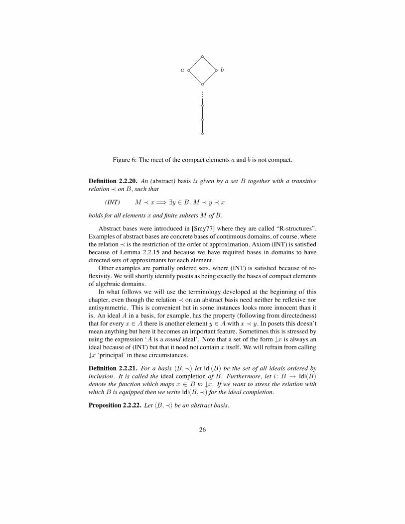
The infimum of compact elements need not be compact again, even in an algebraiclattice. An example is given in Figure 6.

2.2.6 Bases as objects

In Section 2.2.2 we have seen how we can use bases in order to express properties ofthe ambient domain. We will now study the question of how far we can reduce domaintheory to a theory of (abstract) bases. The resulting techniques will prove useful inlater chapters but we hope that they will also deepen the reader’s understanding of thenature of domains.

We start with the question of what additional information is necessary in order toreconstruct a domain from one of its bases. Somewhat surprisingly, it is just the orderof approximation. Thus we define:

25

!!!

!"""

!a ! b

!

!!"

" !!"

"

Figure 6: The meet of the compact elements a and b is not compact.

Definition 2.2.20. An (abstract) basis is given by a set B together with a transitiverelation@ on B, such that

(INT) M @ x =( ?y ! B. M @ y @ x

holds for all elements x and finite subsets M of B.

Abstract bases were introduced in [Smy77] where they are called “R-structures”.Examples of abstract bases are concrete bases of continuous domains, of course, wherethe relation@ is the restriction of the order of approximation. Axiom (INT) is satisfiedbecause of Lemma 2.2.15 and because we have required bases in domains to havedirected sets of approximants for each element.

Other examples are partially ordered sets, where (INT) is satisfied because of re-flexivity. We will shortly identify posets as being exactly the bases of compact elementsof algebraic domains.

In what follows we will use the terminology developed at the beginning of thischapter, even though the relation @ on an abstract basis need neither be reflexive norantisymmetric. This is convenient but in some instances looks more innocent than itis. An ideal A in a basis, for example, has the property (following from directedness)that for every x ! A there is another element y ! A with x @ y. In posets this doesn’tmean anything but here it becomes an important feature. Sometimes this is stressed byusing the expression ‘A is a round ideal’. Note that a set of the form 0x is always anideal because of (INT) but that it need not contain x itself. We will refrain from calling0x ‘principal’ in these circumstances.

Definition 2.2.21. For a basis ,B,@- let Idl(B) be the set of all ideals ordered byinclusion. It is called the ideal completion of B. Furthermore, let i : B " Idl(B)denote the function which maps x ! B to 0x. If we want to stress the relation withwhich B is equipped then we write Idl(B,@) for the ideal completion.

Proposition 2.2.22. Let ,B,@- be an abstract basis.

26

1. The ideal completion of B is a dcpo.

2. A : A% holds in Idl(B) if and only if there are x @ y inB such thatA 1 i(x) 1i(y) 1 A%.

3. Idl(B) is a continuous domain and a basis of Idl(B) is given by i(B).

4. If @ is reflexive then Idl(B) is algebraic.

5. If ,B,@- is a poset then B, K(Idl(B)), and i(B) are all isomorphic.

Proof. (1) holds because clearly the directed union of ideals is an ideal. Roundnessimplies that every A ! Idl(B) can be written as

!

x"A 0x. This union is directedbecause A is directed. This proves (2) and also (3). The fourth claim follows from thecharacterization of the order of approximation. The last clause holds because there isonly one basis of compact elements for an algebraic domain.

Defining the product of two abstract bases as one does for partially ordered sets,we have the following:

Proposition 2.2.23. Idl(B % B%) $= Idl(B) % Idl(B%)

Our ‘completion’ has a weak universal property:

Proposition 2.2.24. Let ,B,@- be an abstract basis and let D be a dcpo. For everymonotone function f : B " D there is a largest continuous function f : Idl(B) " Dsuch that f 5 i is below f . It is given by f(A) =

"

#f(A).

B

!!

!!

f

(Idl(B)

i

' f & D

The assignment f 9" f is a Scott-continuous map from [Bm#" D] to [Idl(B) #" D].

If the relation @ is reflexive then f 5 i equals f .

Proof. Let us first check continuity of f . To this end let (Ai)i"I be a di-rected collection of ideals. Using general associativity (Proposition 2.1.4(3))we can calculate: f(

"

#i"I Ai) = f(

!

i"I Ai) ="

#{f(x) | x !!

i"I Ai} ="

#i"I

"

#{f(x) | x ! Ai} ="

#i"I f(Ai).

Since f is assumed to be monotone, f(x) is an upper bound for f(0x). This provesthat f 5 i is below f . If, on the other hand, g : Idl(B) " D is another continuousfunction with this property then we have g(A) = g(

!

x"A 0x) ="

#x"A g(0x) =

"

#x"A g(i(x)) &

"

#x"A f(x) = f(A).

The claim about the continuity of the assignment f 9" f is shown by the usualswitch of directed suprema.

If@ is a preorder then we can show that f 5i = f : f(i(x)) = f(0x) ="

#f(0x) =f(x).

27

A particular instance of this proposition is the case that B and B% are two abstractbases and f : B " B% is monotone. By the extension of f to Idl(B) we mean the map!i% 5 f : Idl(B) " Idl(B%). It maps an ideal A 1 B to the ideal 0f(A).

Proposition 2.2.25. Let D be a continuous domain with basis B. Viewing ,B,:- asan abstract basis, we have the following:

1. Idl(B) is isomorphic to D. The isomorphism ) : Idl(B) " D is the extension eof the embedding of B into D. Its inverse $ maps elements x ! D to Bx.

2. For every dcpoE and continuous function f : D " E we have f = g 5 $ whereg is the restriction of f to B.

Proof. In a continuous domain we have x ="

#Bx for all elements, so ) 5 $ = idD.Composing the maps the other way round we need to see that every c ! B which ap-proximates

"

#A, whereA is an ideal in ,B,:-, actually belongs toA. We interpolate:c : d :

"

#A and using the defining property of the order of approximation, we finda ! A above d. Therefore c approximates a and belongs to A.

The calculation for (2) is straightforward: f(x) = f("

#Bx) ="

#f(Bx) = g(Bx) = g($(x)).

Corollary 2.2.26. A continuous function from a continuous domain D to a dcpo E iscompletely determined by its behavior on a basis ofD.

As we now know how to reconstruct a continuous domain from its basis and how torecover a continuous function from its restriction to the basis, we may wonder whetherit is possible to work with bases alone. There is one further problem to overcome,namely, the fact that continuous functions do not preserve the order of approximation.The only way out is to switch from functions to relations, where we relate a basiselement c to all basis elements approximating f(c). This can be axiomatized as follows.

Definition 2.2.27. A relation R between abstract bases B and C is called approx-imable if the following conditions are satisfied:

1. >x ! B >y, y% ! C. (xRy A y% =( xRy%);

2. >x ! B >M 1fin C. (>y ! M. xRy =( (?z ! C. xRz and z A M));

3. >x, x% ! B >y ! C. (x% A xRy =( x%Ry);

4. >x ! B >y ! C. (xRy =( (?z ! B. x A zRy)).

The following is then proved without difficulties.

Theorem 2.2.28. The category of abstract bases and approximable relations is equiv-alent to CONT, the category of continuous dcpo’s and continuous maps.

The formulations we have chosen in this section allow us immediately to read offthe corresponding results in the special case of algebraic domains. In particular:

Theorem 2.2.29. The category of preorders and approximable relations is equivalentto ALG, the category of algebraic dcpo’s and continuous maps.

28

2.3 TopologyBy a topology on a space X we understand a system of subsets of X (called the opensets), which is closed under finite intersections and infinite unions. It is an amazingfact that by a suitable choice of a topology we can encode all information about con-vergence, approximation, continuity of functions, and even points ofX themselves. Toa student of Mathematics this appears to be an immense abstraction from the intuitivebeginnings of analysis. In domain theory we are in the lucky situation that we can tieup open sets with the concrete idea of observable properties. This has been done indetail earlier in this handbook, [Smy92], and we may therefore proceed swiftly to themathematical side of the subject.

2.3.1 The Scott-topology on a dcpo

Definition 2.3.1. Let D be a dcpo. A subset A is called (Scott-)closed if it is a lowerset and is closed under suprema of directed subsets. Complements of closed sets arecalled (Scott-)open; they are the elements of )D, the Scott-topology on D.

We shall use the notation Cl(A) for the smallest closed set containingA. Similarly,Int(A) will stand for the open kernel of A.

A Scott-open setO is necessarily an upper set. By contraposition it is characterizedby the property that every directed set whose supremum lies in O has a non-emptyintersection with O.

Basic examples of closed sets are principal ideals. This knowledge is enough toshow the following:

Proposition 2.3.2. Let D be a dcpo.

1. For elements x, y ! D the following are equivalent:

(a) x & y,(b) Every Scott-open set which contains x also contains y,(c) x ! Cl({y}).

2. The Scott-topology satisfies the T0 separation axiom.

3. ,D,)D- is a Hausdorff (= T2) topological space if and only if the order on Dis trivial.

Thus we can reconstruct the order between elements of a dcpo from the Scott-topology. The same is true for limits of directed sets.

Proposition 2.3.3. Let A be a directed set in a dcpo D. Then x ! D is the supremumof A if and only if it is an upper bound for A and every Scott-neighborhood of xcontains an element of A.

Proof. Indeed, the closed set 0"

#A separates the supremum from all other upperbounds of A.

29

Proposition 2.3.4. For dcpo’sD and E, a function f from D to E is Scott-continuousif and only if it is topologically continuous with respect to the Scott-topologies on Dand E.

Proof. Let f be a continuous function from D to E and let O be an open subset of E.It is clear that f&1(O) is an upper set because continuous functions are monotone. Iff maps the element x =

"

#i"I xi ! D into O then we have f(x) = f(

"

#i"I xi) =

"

#i"I f(xi) ! O and by definition there must be some xi which is mapped into O.

Hence f&1(O) is open in D.For the converse assume that f is topologically continuous. We first show that f

must be monotone: Let x & x% be elements of D. The inverse image of the Scott-closed set 0f(x%) contains x%. Hence it also contains x. Now let A 1 D be directed.Look at the inverse image of the Scott-closed set 0(

"

#a"A f(a)). It contains A and is

Scott-closed, too. So it must also contain"

#A. Since by monotonicity f("

#A) is anupper bound of f(A), it follows that f(

"

#A) is the supremum of f(A).

So much for the theme of convergence. Let us now proceed to see in how farapproximation is reflected in the Scott-topology.

2.3.2 The Scott-topology on domains

In this subsection we work with the second-most primitive form of open sets, namelythose which can be written as //x. We start by characterizing the order of approxima-tion.

Proposition 2.3.5. Let D be a continuous domain. Then the following are equivalentfor all pairs x, y ! D:

1. x : y,

2. y ! Int(/x),

3. y ! //x.

Comment: Of course, (1) is equivalent to (3) in all dcpos.

Proposition 2.3.6. Let D be a continuous domain with basis B. Then openness of asubset O of D can be characterized in the following two ways:

1. O =!

x"O//x,

2. O =!

x"O'B//x.

This can be read as saying that every open set is supported by its members from thebasis. We may therefore ask how the Scott-topology is derived from an abstract basis.

Proposition 2.3.7. Let (B,@) be an abstract basis and letM be any subset ofB. Thenthe set {A ! Idl(B) | M * A 8= B} is Scott-open in Idl(B) and all open sets on Idl(B)are of this form.

30

This, finally, nicely connects the theory up with the idea of an observable property.If we assume that the elements of an abstract basis are finitely describable and finitelyrecognisable (and we strongly approve of this intuition) then it is clear how to observea property in the completion: we have to wait until we see an element from a given setof basis elements.

We also have the following sharpening of Proposition 2.3.6:

Lemma 2.3.8. Every Scott-open set in a continuous domain is a union of Scott-openfilters.

Proof. Let x be an element in the open set O. By Proposition 2.3.6 there is an ele-ment y ! O which approximates x. We repeatedly interpolate between y and x. Thisgives us a sequence y : . . . : yn : . . . : y1 : x. The union of all /yn is aScott-open filter containing x and contained in O.

In this subsection we have laid the groundwork for a formulation of Domain The-ory purely in terms of the lattice of Scott-open sets. Since we construe open sets asproperties we have also brought logic into the picture. This relationship will be lookedat more closely in Chapter 7. There and in Section 4.2.3 we will also exhibit moreproperties of the Scott-topology on domains.

Exercises 2.3.9. 1. Formalize the passage from preorders to their quotient posets.

2. Draw line diagrams of the powersets of a one, two, three, and four element set.

3. Show that a poset which has all suprema also has all infima, and vice versa.

4. Refine Proposition 2.1.7 by showing that the fixpoints of a monotone function ona complete lattice form a complete lattice. Is it a sublattice?

5. Show that finite directed sets have a largest element. Characterize the class ofposets in which this is true for every directed set.

6. Show that the directed set of finite subsets of real numbers does not contain acofinal chain.

7. Which of the following are dcpo’s: R, [0, 1] (unit interval), Q, Z& (negativeintegers)?

8. Let f be a monotone map between complete lattices L and M and let A be asubset of L. Prove: f(

"

A) +"

f(A).

9. Show that the category of posets and monotone functions forms a cartesianclosed category.

10. Draw the line diagram for the function space of the flat booleans (see Figure 1).

11. Show that an ideal in a (binary) product of posets can always be seen as theproduct of two ideals from the individual posets.

31

12. Show that a map f between two dcpo’sD and E is continuous if and only if forall directed sets A in D, f(

"

#A) ="

f(A) holds (i.e., monotonicity does notneed to be required explicitly).

13. Give an example of a monotone map f on a pointed dcpo D for which"

#n"N

fn(.) is not a fixpoint. (Some fixpoint must exist by Proposition 2.1.16.)

14. Use fixpoint induction to prove the following. Let f, g : D " D be continuousfunctions on a pointed dcpo D with f(.) = g(.), and f 5 g = g 5 f . Thenfix(f) = fix(g).

15. (Dinaturality of fixpoints) Let D, E be pointed dcpo’s and let f : D "E, g : E " D be continuous functions. Prove

fix(g 5 f) = g(fix(f 5 g)) .

16. Show that Lemma 2.1.21 uniquely characterizes fix among all fixpoint operators.

17. Prove: Given pointed dcpo’sD and E and a continuous function f : D % E "E there is a continuous function Y (f) : D " E such that Y (f) = f 5,idD, Y (f)- holds. (This is the general definition of a category having fixpoints.)How does Theorem 2.1.19 follow from this?

18. Show that each version of the natural numbers as shown in Figure 2 is an exam-ple of a countable dcpo whose function space is uncountable.

19. Characterize the order of approximation on the unit interval. What are the com-pact elements?

20. Show that in finite posets every element is compact.

21. Let L be the lattice of open sets of Q, where Q is equipped with the ordinarymetric topology. Show that no two non-empty open sets approximate each other.Conclude that L is not continuous.

22. Prove Proposition 2.2.10.

23. Extend Proposition 2.2.10 in the following way: For every finite subset M ofa continuous dcpo D with basis B there exists M % 1 B, such that x 9" x% isan order-isomorphism between M and M % and such that for all x ! M , theelement x% belongs to Bx.

24. Prove Proposition 2.2.17.

25. Show that elements of an abstract basis, which approximate no other element,may be deleted without changing the ideal completion.

26. Show that if x is a non-compact element of a basisB for a continuous domainDthen B \ {x} is still a basis. (Hint: Use the interpolation property.)

32

27. The preceding exercise shows that different bases can generate the same do-main. Show that for a fixed basis different orders of approximation may alsoyield the same domain. Show that this will definitely be the case if the two orders@1 and @2 satisfy the equations@15@2 =@1 and @25@1 =@2.

28. Consider Proposition 2.2.22(2). Give an example of an abstract basis B whichshows that i(x) : i(y) in Idl(B) does not entail x @ y.

29. What is the ideal completion of ,Q, <-?

30. Let @ be a relation on a set B such that @5@ = @ holds. Give an exampleshowing that Axiom (INT) (Definition 2.2.20) need not be satisfied. Nevertheless,Idl(B,@) is a continuous domain. What is the advantage of our axiomatizationover this simpler concept?

31. Spell out the proof of Theorem 2.2.28.

32. Prove that in a dcpo every upper set is the intersection of its Scott-neighborhoods.

33. Show that in order to construct the Scott-closure of a lower setA of a continuousdomain it is sufficient to add all suprema of directed subsets to 0A. Give anexample of a non-continuous dcpo where this fails.

34. Given a subsetX in a dcpoD let X be the smallest superset ofX which is closedagainst the formation of suprema of directed subsets. Show that the cardinalityof X can be no greater than 2|X|. (Hint: Construct a directed suprema closedsuperset of X by adding all existing suprema to X .)

33

3 Domains collectively3.1 Comparing domains3.1.1 Retractions

A reader with some background in universal algebra may already have missed a discus-sion of sub-dcpo’s and quotient-dcpo’s. The reason for this omission is quite simple:there is no fully satisfactory notion of sub-object or quotient in domain theory basedon general Scott-continuous functions. And this is because the formation of directedsuprema is a partial operation of unbounded arity. We therefore cannot hope to be ableto employ the tools of universal algebra. But if we combine the ideas of sub-object andquotient then the picture looks quite nice.

Definition 3.1.1. Let P and Q be posets. A pair s : P " Q, r : Q " P of monotonefunctions is called a monotone section retraction pair if r 5 s is the identity on P . Inthis situation we will call P a monotone retract of Q.

If P and Q are dcpo’s and if both functions are continuous then we speak of acontinuous section retraction pair.

We will omit the qualifying adjective ‘monotone’, respectively ‘continuous’, if theproperties of the functions are clear from the context. We will also use s-r-pair as ashorthand.

One sees immediately that in an s-r-pair the retraction is surjective and the sectionis injective, so our intuition about P being both a sub-object and a quotient of Q isjustified. In such a situation P inherits many properties from Q:

Proposition 3.1.2. Let P and Q be posets and let s : P " Q, r : Q " P be a mono-tone section retraction pair.

1. Let A be any subset of P . If s(A) has a supremum in Q then A has a supremumin P . It is given by r(

"

s(A)). Similarly for the infimum.

2. IfQ is a (pointed) dcpo, a semilattice, a lattice or a complete lattice then so is P .

Proof. Because of r 5 s = idP and the monotonicity of r it is clear that r("

s(A))is an upper bound for A. Let x be another such. Then by the monotonicity of s wehave that s(x) is an upper bound of s(A) and hence it is above

"

s(A). So we getx = r(s(x)) + r(

"

s(A)).The property of being a (pointed) dcpo, semilattice, etc., is defined through the ex-

istence of suprema or infima of certain subsets. The shape of these subsets is preservedby monotone functions and so (2) follows from (1).

Let us now turn to continuous section retraction pairs.

Lemma 3.1.3. Let (s, r) be a continuous section retraction pair between dcpo’sD and E and let B be a basis for E. Then r(B) is a basis forD.

34

Proof. Let c ! B be an approximant to s(x) for x ! D. We show that r(c) approxi-mates x. To this end let A be a directed subset of D with

"

#A + x. By the continuityof s we have

"

#s(A) = s("

#A) + s(x) and so for some a ! A, s(a) + c must hold.This implies a = r(s(a)) + r(c). The continuity of r gives us that x is the supremumof r(Bs(x)).

Theorem 3.1.4. A retract of a continuous domain via a continuous s-r-pair is contin-uous.

The analogous statement for algebraic domains does not hold in general. Insteadof constructing a particular counterexample, we use our knowledge about the idealcompletion to get a general, positive result which implies this negative one.

Theorem 3.1.5. Every ("-) continuous domain is the retract of an ("-) algebraic do-main via a continuous s-r-pair.

In more detail, we have:

Proposition 3.1.6. Let D be a continuous domain with basis B. Then the mapss : D " Idl(B,&), x 9" Bx and r : Idl(B,&) " D, A 9"

"

#A constitute a con-tinuous section retraction pair betweenD and Idl(B,&).

Proof. The continuity of r follows from general associativity, Proposition 2.1.4, andthe fact that directed suprema in Idl(B) are directed unions. For the continuity of s weuse the interpolation property in the form of Proposition 2.2.16(2).

3.1.2 Idempotents

Often the section part of an s-r-pair is really a subset inclusion. In this case we can hideit and work with the map s 5 r on E alone. It is idempotent, because (s 5 r) 5 (s 5 r) =s 5 (r 5 s) 5 r = s 5 r.

Proposition 3.1.7. 1. The image of a continuous idempotent map f on a dcpoD isa dcpo. The suprema of directed subsets of im(f), calculated in im(f), coincidewith those calculated in D. The inclusion im(f) " D is Scott-continuous.

2. The set of all continuous idempotent functions on a dcpo is again a dcpo.

Proof. (1) The first part follows from Proposition 3.1.2 because the inclusion is surelymonotone. For the second part let A be a directed set contained in im(f). We need tosee that

"

#A belongs to im(f) again. This holds because f is continuous:"

#A ="

#f(A) = f("

#A).(2) Let (fi)i"I be a directed family of continuous idempotents. For any x ! D we

35

can calculate

($

#

i"I

fi) 5 ($

#

j"I

fj)(x) =$

#

i"I

fi($

#

j"I

fj(x))

=$

#

i"I

$

#

j"I

fi(fj(x))

=$

#

i"I

fi(fi(x))

=$

#

i"I

fi(x).

Hence the supremum of continuous idempotents is again an idempotent function. Wehave proved in Proposition 2.1.18 that it is also continuous.

If f is a continuous idempotent map on a continuous domain D then we knowthat its image is again continuous. But it is not true that the order of approximationon im(f) is the restriction of the order of approximation on D. For example, everyconstant map is continuous and idempotent. Its image is an algebraic domain with oneelement, which is therefore compact. But surely not every element of a continuousdomain is compact. However, we can say something nice about the Scott-topology onthe image:

Proposition 3.1.8. If f is a continuous idempotent function on a dcpo D then theScott-topology on im(f) is the restriction of the Scott-topology onD to im(f).

Proof. This follows immediately because a continuous idempotent function f givesrise to a continuous s-r-pair between im(f) andD.

Useful examples of idempotent self-maps are retractions retx onto principal ideals.They are given by

retx(y) =

&

y, if y & x;x, otherwise.

Their continuity follows from the fact that 0x is always Scott-closed. Dually, we candefine a retraction onto a principal filter /c. It is Scott-continuous if (but not only if)its generator c is compact.

3.1.3 Adjunctions

An easy way to avoid writing this subsection would be to refer to category theory and totranslate the general theory of adjoint functors into the poset setting. However, we feelthat the right way to get used to the idea of adjointness is to start out with a relativelysimple situation such as is presented by domain theory. (In fact, we will use adjointfunctors later on, but really in a descriptive fashion only.)

Let us start with the example of a surjective map f from a poset Q onto a poset P .It is natural to ask whether there is a one-sided inverse e : P " Q for f , i.e. a mapsuch that f 5 e = idP holds. Figure 7 illustrates this situation. Such a map must

36

'a

'b

'c)))

)))f&1(a)

f&1(b)

f&1(c)f

?

*

&

(

)

*

+

(

)

*

+Figure 7: The right inverse problem for a surjective function

pick out a representative from f&1(x) for each x ! P . Set-theoretically this can bedone, but the point here is that we want e to be monotone. If we succeed then e and fform a (monotone) section retraction pair. Even nicer would it be if we could pickout a canonical representative from f&1(x), which in the realm of order theory meansthat we want f&1(x) to have a least (or largest) element. If this is the case then howcan we ensure that the assignment e : x 9" min(f&1(x)) is monotone? The solutionis suggested by the observation that if e is monotone then e(x) is not only the leastelement of f&1(x) but also of f&1(/x). This condition is also sufficient. The switchfrom f&1(x) to f&1(/x) (and this is a trick to remember) may allow us to constructa partial right inverse even if f is not surjective. Thus we arrive at a first, tentativedefinition of an adjunction.

Definition 3.1.9. (preliminary) Let P andQ be posets and let l : P " Q and u : Q "P be monotone functions. We say that (l, u) is an adjunction between P and Q if forevery x ! P we have that l(x) is the least element of u&1(/x).

This definition is simple and easy to motivate. But it brings out just one aspect ofadjoint pairs, namely, that l is uniquely determined by u. There is much more:

Proposition 3.1.10. Let P and Q be posets and l : P " Q and u : Q " P be mono-tone functions. Then the following are equivalent:

1. >x ! P. l(x) = min(u&1(/x)),

2. >y ! Q. u(y) = max(l&1(0y)),

3. l 5 u & idQ and u 5 l + idP ,

4. >x ! P >y ! Q. (x & u(y) ; l(x) & y).

(For (4)=((1) the monotonicity of u and l is not needed.)

Proof. (1)=((2) Pick an element y ! Q. Then because u(y) & u(y)we have from (1)that l(u(y)) & y holds. So u(y) belongs to l&1(0y). Now let x% be any element ofl&1(0y), or, equivalently, l(x%) & y. Using (1) again, we see that this can only happenif u(y) + x% holds. So u(y) is indeed the largest element of l&1(0y). The converse isproved analogously, of course.

(1) and (2) together immediately give both (3) and (4).From (3) we get (4) by applying the monotone map l to the inequality x & u(y)

and using l 5 u & idQ.

37

Assuming (4) we see immediately that l(x) is a lower bound for u&1(/x). Butbecause l(x) & l(x) and hence x & u(l(x))we have that l(x) also belongs to u&1(/x).We get the monotonicity of l as follows: If x & x% holds in P then because l(x%) &l(x%) we have x% & u(l(x%)) and by transitivity x & u(l(x%)). Using (4) again, we getl(x) & l(x%).

We conclude that despite the lopsided definition, the situation described by an ad-junction is completely symmetric. And indeed, adjunctions are usually introduced us-ing either (3) or (4).

Definition 3.1.11. (official) Let P and Q be posets and let l : P " Q and u : Q " Pbe functions. We say that (l, u) is an adjunction between P and Q if for all x ! P andy ! Q we have x & u(y) ; l(x) & y. We call l the lower and u the upper adjoint andwrite l : P ! Q : u.

Proposition 3.1.12. Let l : P ! Q : u be an adjunction between posets.

1. u 5 l 5 u = u and l 5 u 5 l = l,

2. The image of u and the image of l are order-isomorphic. The isomorphisms aregiven by the restrictions of u and l to im(l) and im(u), respectively.

3. u is surjective; u 5 l = idP ; l is injective,

4. l is surjective; l 5 u = idQ ; u is injective,

5. l preserves existing suprema, u preserves existing infima.

Proof. (1) We use Proposition 3.1.10(3) twice: u = idP 5u & (u5 l)5u = u5(l5u) &u 5 idQ = u.

(2) The equations from (1) say precisely that on the images of u and l, u 5 l andl 5 u, respectively, act like identity functions.

(3) If u is surjective then we can cancel u on the right in the equation u 5 l 5 u = uand get u 5 l = idP . From this it follows that l must be injective.

(5) Let x ="

A for A 1 P . By monotonicity, l(x) + l(a) for each a ! A.Conversely, let y be any upper bound of l(A). Then u(y) is an upper bound for eachu(l(a)) which in turn is above a. So u(y) +

"

A = x holds and this is equivalent toy + l(x).

The last property in the preceding proposition may be used to define an adjunc-tion in yet another way, the only prerequisite being that there are enough sets with aninfimum (or supremum). This is the Adjoint Functor Theorem for posets.

Proposition 3.1.13. Let f : L " P be a monotone function from a complete lattice toa poset. Then the following are equivalent:

1. f preserves all infima,

2. f has a lower adjoint.

And similarly: f preserves all suprema if and only if f has an upper adjoint.

38

Proof. We already know how to define a candidate for a lower adjoint g; we try g(x) =!f&1(/x). All that remains, is to show that g(x) belongs to f&1(/x). This follows

because f preserves meets: f(g(x)) = f(!

f&1(/x)) =!

f(f&1(/x)) +!/x =

x.

This proposition gives us a way of recognizing an adjoint situation in cases whereonly one function is explicitly given. It is then useful to have a notation for the missingmapping. We write f( for the upper and f( for the lower adjoint of f .

Now it is high time to come back to domains and see what all this means in oursetting.

Proposition 3.1.14. Let l : D ! E : u be an adjunction between dcpo’s.

1. l is Scott-continuous.

2. If u is Scott-continuous then l preserves the order of approximation.

3. If D is continuous then the converse of (2) is also true.

Proof. Continuity of the lower adjoint follows from Proposition 3.1.12(5). So let x :y be elements in D and let A be a directed subset of E such that l(y) &

"

#A holds.This implies y & u(

"

#A) and from the continuity of u we deduce y &"

#u(A).Hence some u(a) is above x which, going back to E, means l(x) & a.

(3) For the converse let A be any directed subset of E. Monotonicity of u yields"

#u(A) & u("

#A). In order to show that the other inequality also holds, we provethat

"

#u(A) is above every approximant to u("

#A). Indeed, if x : u("

#A)we havel(x) : l(u(

"

#A)) &"

#A by assumption. So some a is above l(x) and for this a wehave x & u(a) &

"

#u(A).

3.1.4 Projections and sub-domains

Let us now combine the ideas of Section 3.1.1 and 3.1.3.

Definition 3.1.15. Let D and E be dcpo’s and let e : D " E and p : E " D becontinuous functions. We say that (e, p) is a continuous embedding projection pair (ore-p-pair) if p 5 e = idD and e 5 p & idE .

We note that the section retraction pair between a continuous domain and its idealcompletion as constructed in Section 3.1.1 is really an embedding projection pair.

From the general theory of adjunctions and retractions we already know quite abit about e-p-pairs. The embedding is injective, p is surjective, e preserves existingsuprema and the order of approximation, p preserves existing infima, D is continuousif E is continuous, and, finally, embeddings and projections uniquely determine eachother. Because of this last property the term ‘embedding’ has a well-defined meaning;it is an injective function which has a Scott-continuous upper adjoint.

An injective lower adjoint also reflects the order of approximation:

Proposition 3.1.16. Let e : D ! E : p be an e-p-pair between dcpo’s and let x and ybe elements of D. Then e(x) : e(y) holds in E if and only if x approximates y in D.

39

Let us also look at the associated idempotent e5p onE. As it is below the identity, itmakes good sense to call such a function a kernel operator, but often such maps are justcalled projections. We denote the set of kernel operators on a dcpo D by [D

)#" D].

It is important to note that while a kernel operator preserves infima as a map fromD toits image, it does not have any preservation properties as a map from D to D besidesScott-continuity. What we can say is summarized in the following proposition.

Proposition 3.1.17. Let D be a dcpo.

1. [D)

#" D] is a dcpo.

2. If p is a kernel operator on D then for all x ! D we have that p(x) = max{y !im(p) | y & x}.

3. The image of a kernel operator is closed under existing suprema.

4. :im(p)= (:D) * (im(p) % im(p)).

5. For kernel operators p, p% on D we have p & p% if and only if im(p) 1 im(p%).

Proof. (1) is proved as Proposition 3.1.7 and (2) follows because p together with theinclusion of im(p) intoD form an adjunction. This also shows (4). Finally, (3) and (5)are direct consequences of (2).

In the introduction we explained the idea that the order on a semantic domainmodels the relation of some elements being better than others, where—at least insemantics—‘better’ may be replaced more precisely by ‘better termination’. Thus weview elements at the bottom of a domain as being less desirable than those higher up;they are ‘proto-elements’ from which fully developed elements evolve as we go up inthe order. Now, the embedding part of an e-p-pair e : D ! E : p places D at the bot-tom ofE. Following the above line of thought, we may think ofD as being a collectionof proto-elements from which the elements of E evolve. Because there is the projec-tion part as well, every element of E exists in some primitive form in D already. Also,D contains some information about the order and the order of approximation on E.We may therefore think of D as a preliminary version of E, as an approximation to Eon the domain level. This thought is made fruitful in Sections 4.2 and 5. Although theword does not convey the whole fabric of ideas, we name D a sub-domain of E, justin case there is an e-p-pair e : D ! E : p.

3.1.5 Closures and quotient domains

The sub-domain relation is preeminent in domain theory but, of course, we can alsocombine retractions and adjunctions the other way around. Thus we arrive at contin-uous insertion closure pairs (i-c-pairs). Because adjunctions are not symmetric as faras the order of approximation is concerned, Proposition 3.1.14, the situation is not justthe order dual of that of the previous subsection. We know that the insertion preservesexisting infima and so on, but in addition we now have that the surjective part preservesthe order of approximation and therefore, D is algebraic if E is.

40

The associated idempotent is called a closure operator. For closure operators thesame caveat applies as for kernel operators; they need not preserve suprema. Worse,such functions do no longer automatically have a Scott-continuous (upper) adjoint.This is the price we have to pay for the algebraicity of the image. Let us formulate thisprecisely.

Proposition 3.1.18. Let D be an algebraic domain and let c : D " D be a monotoneidempotent function above idD . Then im(c) is again an algebraic domain if and only ifit is closed under directed suprema.

The reader will no doubt recognize this statement as being a reformulation andgeneralization of our example of inductive closure systems from Chapter 2, Proposi-tion 2.2.9. It is only consequent to callD a quotient domain of the continuous domainE if there exists an i-c-pair e : D " E : c.

3.2 Finitary constructionsIn this section we will present a few basic ways of putting domains together so as tobuild up complicated structures from simple ones. There are three aspects of theseconstructions which we are interested in. The first one is simply the order-theoreticdefinition and the proof that we stay within dcpo’s and Scott-continuous functions.The second one is the question how the construction can be described in terms of basesand whether the principle of approximation can be retained. The third one, finally, isthe question of what universal property the construction has. This is the categoricalviewpoint. Since this Handbook contains a chapter on category theory, [Poi92] (inparticular, Chapter 2), we need not repeat here the arguments for why this is a fruitfuland enlightening way of looking at these type constructors.

There are, however, several categories that we are interested in and a constructionmay play different roles in different settings. Let us therefore list the categories that,at this point, seem suitable as a universe of discourse. There is, first of all, DCPO, thecategory of dcpo’s and Scott-continuous functions as introduced in Section 2.1. Wecan restrict the objects by taking only continuous or, more special, algebraic domains.Thus we arrive at the full subcategories CONT and ALG of DCPO. Each of thesemay be further restricted by requiring the objects to have a bottom element (and Theo-rem 2.1.19 tells us why one would be interested in doing so) resulting in the categoriesDCPO$, CONT$, and ALG$. The presence of a distinguished point in each objectsuggests that morphisms should preserve them. But this is not really appropriate insemantics; strict functions are tied to a particular evaluation strategy. For us this meansthat there is yet another cascade of categories,DCPO$!, CONT$!, andALG$!, whereobjects have bottom elements and morphisms are strict and Scott-continuous. Finally,we may bound the size of (minimal) bases for continuous and algebraic domains to becountable. We indicate this by the prefix ‘"-’.

41

3.2.1 Cartesian product

Definition 3.2.1. The cartesian product of two dcpo’sD andE is given by the followingdata:

D % E = {,x, y- | x ! D, y ! E},

,x, y- & ,x%, y%- if and only if x & x% and y & y%.

This is just the usual product of sets, augmented by the coordinatewise order.Through induction, we can define the cartesian product for finite non-empty collec-tions of dcpo’s. For the product over the empty index set we define the result to be afixed one-element dcpo I.

Proposition 3.2.2. The cartesian product of dcpo’s is a dcpo. Suprema and infima arecalculated coordinatewise.

With each productD % E there are associated two projections:

*1 : D % E " D and *2 : D % E " E.

These projections are always surjective but they are upper adjoints only ifD and E arepointed. So there is a slight mismatch with Section 3.1.4 here. Given a dcpo F andcontinuous functions f : F " D and g : F " E, we denote the mediating morphismfrom F toD % E by ,f, g-. It maps x ! F to ,f(x), g(x)-.

Proposition 3.2.3. Projections and mediating morphisms are continuous.

If f : D " D% and g : E " E% are Scott-continuous, then so is the mediating map,f 5 *1, g 5 *2- : D % E " D% % E%. The common notation for it is f % g. Sinceour construction is completely explicit, we have thus defined a functor in two variableson DCPO.

Proposition 3.2.4. Let D and E be dcpo’s.

1. A tuple ,x, y- approximates a tuple ,x%, y%- inD%E if and only if x approximatesx% in D and y approximates y% in E.

2. If B and B% are bases for D and E, respectively, then B % B% is a basis forD % E.

3. D % E is continuous if and only if D and E are.

4. K(D % E) = K(D) % K(E).

The categorical aspect of the cartesian product is quite pleasing; it is a categoricalproduct in each case. But we can say even more.

Lemma 3.2.5. Let C be a full subcategory of DCPO or DCPO$! which has finiteproducts. Then these are isomorphic to the cartesian product.

42

In a restricted setting this was first observed in [Smy83a]. The general proof maybe found in [Jun89].

A useful property which does not follow from general categorical or topologicalconsiderations, is the following.

Lemma 3.2.6. A function f : D % E " F is continuous if and only if it is continuousin each variable separately.

Proof. Assume f : D % E " F is separately continuous. Then f is monotone, be-cause given (x, y) & (x%, y%) we can fill in (x, y%) and use coordinatewise monotonicitytwice. The same works for continuity: if A 1 D % E is directed then

$

#

(x,y)"A

f(x, y) =$

#

x"!1(A)

$

#

y"!2(A)

f(x, y)

=$

#

x"!1(A)

f(x,$

#

y"!2(A)

y)

= f($

#

x"!1(A)

x,$

#

y"!2(A)

y)

= f($

#A).

This proves the interesting direction.

3.2.2 Function space

We have introduced the function space in Section 2.1.6 already. It consists of allcontinuous functions between two dcpo’s ordered pointwise. We know that thisis again a dcpo. The first morphism which is connected with this construction isapply : [D #" E] % D " E, ,f, x- 9" f(x). It is continuous because it is contin-uous in each argument separately: in the first because directed suprema of functionsare calculated pointwise, in the second, because [D #" E] contains only continuousfunctions.

The second standard morphism is the operation which rearranges a function of twoarguments into a combination of two unary functions. That is, if f maps D % E to F ,then Curry(f) : D " [E #" F ] is the mapping which assigns to d ! D the functionwhich assigns to e ! E the element f(d, e). Curry(f) is a continuous function becauseof Lemma 3.2.6. And for completely general reasons we have that Curry itself is acontinuous operation from [D % E #" F ] to [D #" [E #" F ]]. Another derivedoperation is composition which is a continuous operation from [D #" E]%[E #" F ]to [D #" F ].

All this shows that the continuous function space is the exponential in DCPO.Taking cartesian products and function spaces together we have shown that DCPO iscartesian closed.

We turn the function space construction into a functor from DCPOop % DCPO toDCPO by setting [· #" ·](f, g)(h) = g 5 h 5 f , where f : D% " D, g : E " E% andh is an element of [D #" E].

43

++

++

++

+++ ,

,,,,,------ .

..

..

..

..

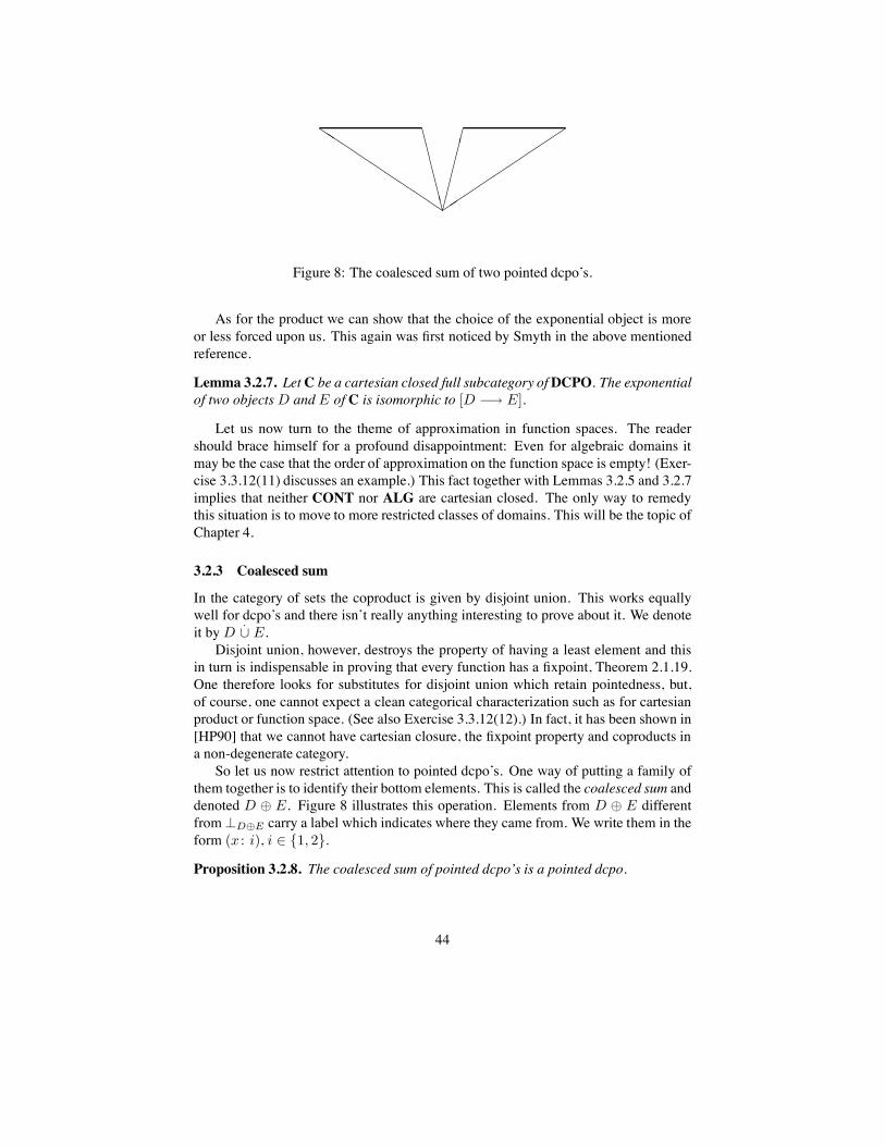
Figure 8: The coalesced sum of two pointed dcpo’s.

As for the product we can show that the choice of the exponential object is moreor less forced upon us. This again was first noticed by Smyth in the above mentionedreference.

Lemma 3.2.7. LetC be a cartesian closed full subcategory ofDCPO. The exponentialof two objectsD and E of C is isomorphic to [D #" E].

Let us now turn to the theme of approximation in function spaces. The readershould brace himself for a profound disappointment: Even for algebraic domains itmay be the case that the order of approximation on the function space is empty! (Exer-cise 3.3.12(11) discusses an example.) This fact together with Lemmas 3.2.5 and 3.2.7implies that neither CONT nor ALG are cartesian closed. The only way to remedythis situation is to move to more restricted classes of domains. This will be the topic ofChapter 4.

3.2.3 Coalesced sum

In the category of sets the coproduct is given by disjoint union. This works equallywell for dcpo’s and there isn’t really anything interesting to prove about it. We denoteit byD

.6 E.

Disjoint union, however, destroys the property of having a least element and thisin turn is indispensable in proving that every function has a fixpoint, Theorem 2.1.19.One therefore looks for substitutes for disjoint union which retain pointedness, but,of course, one cannot expect a clean categorical characterization such as for cartesianproduct or function space. (See also Exercise 3.3.12(12).) In fact, it has been shown in[HP90] that we cannot have cartesian closure, the fixpoint property and coproducts ina non-degenerate category.

So let us now restrict attention to pointed dcpo’s. One way of putting a family ofthem together is to identify their bottom elements. This is called the coalesced sum anddenoted D C E. Figure 8 illustrates this operation. Elements from D C E differentfrom.D*E carry a label which indicates where they came from. We write them in theform (x : i), i ! {1, 2}.

Proposition 3.2.8. The coalesced sum of pointed dcpo’s is a pointed dcpo.

44

The individual dcpo’s may be injected into the sum in the obvious way:

inl(x) =

&

(x : 1), x 8= .D;.D*E, x = .D

;

andinr(x) =

&

(x : 2), x 8= .E;.D*E, x = .E

.

A universal property for the sum holds only in the realm of strict functions:

Proposition 3.2.9. The coalesced sum of pointed dcpo’s is the coproduct in DCPO$!,CONT$!, and ALG$!.

Once we accept the restriction to bottom preserving functions it is clear how to turnthe coalesced sum into a functor.

3.2.4 Smash product and strict function space

It is clear that inside DCPO$! a candidate for the exponential is not the full functionspace but rather the set [D $!

#" E] of strict continuous functions from D to E. How-ever, it does not harmonize with the product in DCPO$!, which, as we have seen, mustbe the cartesian product. We do get a match if we consider the so-called smash product.It is defined like the cartesian product but all tuples which contain at least one bottomelement are identified. Common notation isD D E.

We leave it to the reader to check that smash product and strict function space turnDCPO$! into a monoidal closed category.

3.2.5 Lifting

Set-theoretically, lifting is the simple operation of adding a new bottom element to adcpo. Applied to D, the resulting structure is denoted by D$. Clearly, continuity oralgebraicity don’t suffer any harm from this.

Associated with it is the map up : D " D$ which maps each x ! D to its name-sake in D$.

The categorical significance of lifting stems from the fact that it is left adjoint tothe inclusion functor from DCPO$! into DCPO. (Where a morphism f : D " E islifted by mapping the new bottom element ofD$ to the new bottom element of E$.)

3.2.6 Summary

For quick reference let us compile a table of the constructions looked at so far. A ‘#’indicates that the category is closed under the respective construction, a ‘+’ says that, inaddition, the construction plays the expected categorical role as a product, exponentialor coproduct, respectively. Observe that for the constructions considered in this sectionit makes no difference if we restrict the size of a (minimal) basis.

45

DCPO DCPO! DCPO!! CONT ALGCONT!ALG!

CONT!!ALG!!

D % E + + + + + +[D #" E] + + #

D.6 E + +

D D E # # # #

[D$!#" E] # +D C E # + # +

D$ # # # # # #

3.3 Infinitary constructionsThe product and sum constructions from the previous section have infinitary counter-parts. Generally, these work nicely as long as we are only concerned with questionsof convergence, but they cause problems with respect to the order of approximation.This is exemplified by the fact that an infinite power of a finite poset may fail to bealgebraic. In any case, there is not much use of these operations in semantics. Muchmore interesting is the idea of incrementally building up a domain in a limit process.This is the topic of this section.

3.3.1 Limits and colimits

Our limit constructions are to be understood categorically and hence we refer oncemore to [Poi92] for motivation and general results. Here are the basic defini-tions. A diagram in a category C is given by a functor from a small category Ito C. We can describe, somewhat sloppily but more concretely, a diagram by a pair,(Di)i"O, (fj : Dd(j) " Dc(j))j"M - of a family of objects and a family of connect-ing morphisms. The shape of the diagram is thus encoded in the index sets O (whichcorrespond to the objects of I) and M (which correspond to the morphisms of I) andin the maps c, d : M " O which corresponds to the dom and codom map on I. Whatis lost is the information about composition in I. In the cases which interest us, thisis not a problem. A cone over such a diagram is given by an object D and a fam-ily (fi : D " Di)i"O of morphisms such that for all j ! M we have fj 5fd(j) = fc(j).A cone is limiting if for every other cone ,E, (gi)i"O- there is exactly one morphismf : E " D such that for all i ! O, gi = fi 5 f . If ,D, (fi)i"O- is a limiting cone,then D is called limit and the fi are called limiting morphisms. The dual notions arecocone, colimit, and colimiting morphism.

Theorem 3.3.1. DCPO has limits of arbitrary diagrams.

Proof. The proof follows general category theoretic principles. We describe the limitof the diagram ,(Di)i"O, (fj : Dd(j) " Dc(j))j"M - as a set of particular elements ofthe product of all Di’s, the so-called commuting tuples.

D = {,xi : i ! O- !'

i"O

Di | >j ! M. xc(j) = fj(xd(j))}

46

! ,! !

,, ,

! ! ! !! !

,, ,

, , , ,, ,! ! !! ! ! !

//

// 00

00

!!

##$$ 111 222 %

%222

%%

333----

!!

##$$ 111 222 %

%222

%%

333----

$$%

%4455 6677

Figure 9: An expanding sequence of finite domains.

The order on the limit object is inherited from the product, that is, tuples are orderedcoordinatewise. It is again a dcpo because the coordinatewise supremumof commutingtuples is commuting as all fj are Scott-continuous. This also proves that the projections*j :

(

i"O Di " Dj restricted to D are continuous. They give us the maps needed tocomplementD to a cone.

Given any other cone ,E, (gi : E " Di)i"O-, we define the mediating morphismh : E " D by h(x) = ,gi(x) : i ! O-. Again, it is obvious that this is well-definedand continuous, and that it is the only possible choice.

We also have the dual:

Theorem 3.3.2. DCPO has colimits of arbitrary diagrams.

This was first noted in [Mar77] and, for a somewhat different setting, in [Mes77].The simplest way to prove it is by reducing it to completeness a la Theorem 23.14of [HS73]. This appears in [LS81]. A more detailed analysis of colimits appears in[Fie92]. There the problem of retaining algebraicity is also addressed.

Theorem 3.3.3. DCPO is cartesian closed, complete and cocomplete.

Theorem 3.3.4. DCPO$! is monoidal closed, complete and cocomplete.

How about DCPO$, where objects have least elements but morphisms need notpreserve them? The truth is that both completeness and cocompleteness fail for thiscategory. On the other hand, it is the right setting for denotational semantics in mostcases. As a result of this mismatch, we quite often must resort to detailed proofs onthe element level and cannot simply apply general category theoretic principles. Let usnevertheless write down the one good property of DCPO$:

Theorem 3.3.5. DCPO$ is cartesian closed.

3.3.2 The limit-colimit coincidence

The theorems of the previous subsection fall apart completely if we pass to domains,that is, to CONT or ALG. To get better results for limits and colimits we must restrictboth the shape of the diagrams and the connecting morphisms used.

47

For motivation let us look at a chain D1, D2, . . . of domains where each Dn isa sub-domain of Dn+1 in the sense of Section 3.1.4. Taking up again the animatedlanguage from that section we may think of the points of Dn+1 as growing out ofpoints ofDn, the latter being the buds which contain the leaves and flowers to be seenat later stages. Figure 9 shows a, hopefully inspiring, example. Intuition suggests thatin such a situation a well-structured limit can be found by adding limit points to theunion of theDn, and that it will be algebraic if theDn are.

Definition 3.3.6. A diagram ,(Dn)n"N, (emn : Dn " Dm)n+m"N- in the categoryDCPO is called an expanding sequence, if the following conditions are satisfied:

1. Each emn : Dn " Dm is an embedding. (The associated projection e(mn wedenote by pnm.)

2. >n ! N. enn = idDn.

3. >n ) m ) k ! N. ekn = ekm 5 emn .

Note that because lower adjoints determine upper adjoints and vice versa, we havepnk = pnm 5 pmk whenever n ) m ) k ! N.

It turns out that, in contrast to the general situation, the colimit of an expandingsequence can be calculated easily via the associated projections.

Theorem 3.3.7. Let ,(Dn)n"N, (emn : Dn " Dm)n+m"N- be an expanding sequencein DCPO. Define

D = {,xn : n ! N- !(

n"NDn | >n ) m ! N. xn = pnm(xm)},

pm : D " Dm, ,xn : n ! N- 9" xm, m ! N,

em : Dm " D, x 9" ,"

#k,n,m pnk 5 ekm(x) : n ! N-, m ! N .3

Then

1. The maps (em, pm), m ! N, form embedding projection pairs and"

#m"N

em 5pm = idD holds.

2. ,D, (pn)n"N- is a limit of the diagram ,(Dn)n"N, (pnm)n+m"N-. If,C, (gn)n"N- is another cone, then the mediating map from C to D is givenby g(x) = ,gn(x) : n ! N- or g =

"

#n"N

en 5 gn.

3. ,D, (en)n"N- is a colimit of the diagram ,(Dn)n"N, (emn)n+m"N-. If,E, (fn)n"N- is another cocone, then the mediating map from D to E is givenby f(,xn : n ! N-) =

"

#n"N

fn(xn) or f ="

#n"N

fn 5 pn.

Proof. We have already shown in Theorem 3.3.1 that a limit of the diagram,(Dn), (pnm)- is given by ,D, (pn)- and that the mediating morphism has the (first)postulated form.

3he directed supremumF

!k"n,m pnk ! ekm(x) in the definition of em could be replaced by pnk !

ekm(x) for any upper bound k of {n, m} in N. However, this would actually make the proofs more cum-bersome to write down.

48

For the rest, let us start by showing that the functions em are well-defined, i.e. thaty = em(x) is a commuting tuple. Assume n ) n%. Then we have pnn"(yn") =pnn"(

"

#k,n",m pn"k 5 ekm(x)) =

"

#k,n",m pnn" 5 pn"k 5 ekm(x) =

"

#k,n",m pnk 5

ekm(x) = yn. The assignment x 9" em(x) is Scott-continuous because of generalassociativity and because only Scott-continuous maps are involved in the definition.

Next, let us now check that em and pm form an e-p-pair.

em 5 pm(,xn : n ! N-) = em(xm)

= ,"

#k,n,m pnk 5 ekm(xm) : n ! N-

= ,"

#k,n,m pnk 5 ekm 5 pmk(xk) : n ! N-

& ,"

#k,n,m pnk(xk) : n ! N-

= ,xn : n ! N-

and pm 5 em(x) = pm(,"

#k,n,m pnk 5 ekm(x) : n ! N-) =

"

#k,m pmk 5 ekm(x) =

x.A closer analysis reveals that em 5 pm will leave all those elements of the tuple

,xn : n ! N- unchanged for which n ) m:

pn(em 5 pm(,xn : n ! N-)) = . . . =$

#

k-n,m

pnk 5 ekm 5 pmk(xk)

=$

#

k-n,m

pnm 5 pmk 5 ekm 5 pmk(xk)

=$

#

k-n,m

pnm 5 pmk(xk) =$

#

k-n,m

xn = xn

This proves that the em5pm,m ! N, add up to the identity, as stated in (1). Putting thisto use, we easily get the second representation for the mediating map intoD viewed asa limit: g = id 5 g =

"

#m"N

em 5 pm 5 g ="

#m"N

em 5 gm.It remains to prove the universal property of D as a colimit. To this end let

,E, (fn)n"N- be a cocone over the expanding sequence. We have to check thatf =

"

#n"N

fn 5 pn is well-defined in the sense that the supremum is over a directedset. So let n ) m. We get fn 5 pn = fm 5 emn 5 pnm 5 pm & fm 5 pm. It commuteswith the colimiting maps because

f 5 em =$

#

n-m

fn 5 pn 5 em

=$

#

n-m

fn 5 pn 5 en 5 enm

=$

#

n-m

fn 5 enm =$

#

n-m

fm = fm

We also have to show that there is no other choice for f . Again the equation in (1)comes in handy: Let f % be any mediating morphism. It must satisfy f % 5 em = fm

and so f % 5 em 5 pm = fm 5 pm. Forming the supremum on both sides gives f % ="

#m"N

fm 5 pm which is the definition of f .

49

This fact, that the colimit of an expanding sequence is canonically isomorphic tothe limit of the associated dual diagram, is called the limit-colimit coincidence. It isone of the fundamental tools of domain theory and plays its most prominent role inthe solution of recursive domain equations, Chapter 5. Because of this coincidence wewill henceforth also speak of the bilimit of an expanding sequence and denote it bybilim,(Dn), (emn)-.

We can generalize Theorem 3.3.7 in two ways; we can replace N by an arbitrarydirected set (in which case we will speak of an expanding system) and we can usegeneral Scott-continuous adjunctions instead of e-p-pairs. The first generalization isharmless and does not need any serious adjustments in the proofs. We will freely useit from now on. The second, on the other hand, is quite interesting. By the passagefrom embeddings to, no longer injective, lower adjoints, we allow domains not only togrow but also to shrink as we move on in the index set. Thus points, which at somestage looked different, may at a later stage be recognised to be the same. The interestedreader will find an outline of the mathematical theory of this in the exercises. For themain text, we must remind ourselves that this generalization has so far not found anyapplication in semantics.

Part (1) of the preceding theorem gives a characterization of bilimits:

Lemma 3.3.8. Let ,E, (fn)n"N- be a cocone for the expanding sequence,(Dn)n"N,(emn : Dn " Dm)n+m"N-. It is colimiting if and only if, firstly, thereare Scott-continuous functions gn : E " Dn such that each (fn, gn) is an e-p-pairand, secondly,

"

#n"N

fn 5 gn = idE holds.

Proof. Necessity is Part (1) of Theorem 3.3.7. For sufficiency we show that thebilimitD as constructed there, is isomorphic to E. We already have maps f : D " Eand g : E " D because D is the bilimit. These commute with the limiting and thecolimiting morphisms, respectively. So let us check that they compose to identities:

f 5 g(x) = f(,gn(x) : n ! N-)

=$

#

n"N

fn 5 gn(x)

= x

and

g 5 f = ($

#

n"N

en 5 gn) 5 ($

#

m"N

fm 5 pm)

=$

#

n"N

en 5 gn 5 fn 5 pn

=$

#

n"N

en 5 pn = idD.

We note that in the proof we have used the condition"

#n"N

fn 5 gn = idE onlyfor the first calculation. Without it, we still get that f and g form an e-p-pair. Thus wehave:

50

Proposition 3.3.9. Let ,E, (fn)n"N- be a cocone over the expanding sequence,(Dn)n"N, (emn : Dn " Dm)n+m"N- where the fn are embeddings. Then the bilimitof the sequence is a sub-domain of E.

In other words:

Corollary 3.3.10. The bilimit of an expanding sequence is also the colimit (limit) inthe restricted category of dcpo’s with embeddings (projections) as morphisms.

3.3.3 Bilimits of domains

Theorem 3.3.11. Let ,(Dn)n"N, (emn : Dn " Dm)n+m"N- be an expanding se-quence and ,D, (en)n"N- its bilimit.

1. If all Dn are ("-)continuous then so is D. If we are given bases Bn, n ! N foreach Dn then a basis forD is given by

!

n"Nen(Bn).

2. If all Dn are ("-)algebraic then so is D and K(D) =!

n"Nen(K(Dn)).

Proof. Given an element x ! D we first show that!

n"Nen(Bn

pn(x)) is directed. Tothis end it is sufficient to show that for all n ) m ! N and for each y ! Bn

pn(x) there isy% ! Bm

pm(x) with en(y) & em(y%). Well, because y approximates pn(x) and becauseembeddings preserve the order of approximation, we have emn(y) : emn(pn(x)) =emn(pnm 5 pm(x)) & pm(x). Since pm(x) =

"

#Bmpm(x), some y% : pm(x) is

above emn(y). This implies en(y) = em(emn(y)) & em(y%).The set

!

n"Nen(Bn

pn(x)) gives back x because x ="

#n"N

en 5 pn(x) ="

#n"N

en("

#Bnpn(x)) =

"

#n"N

"

#en(Bnpn(x)) =

"

#!

en(Bnpn(x)). It consists

solely of approximants to x because the en are lower adjoints.

Exercises 3.3.12. 1. Let D be a continuous domain and let f : D " D be anidempotent Scott-continuous function. Show that f(x) : f(y) holds in theimage of f if and only if there exists z : f(y) in D such that f(x) & f(z) &f(y). In the case that D is algebraic conclude that an element x of im(f) iscompact if and only if there is c ! K(D)f(x) with f(c) = f(x).

2. Let p be a kernel operator with finite image. Show that im(p) is containedin K(D) and that p itself is compact in [D #" D].

3. [Hut92] A chain C is called order dense if it has more than one element and foreach pair x $ y there exists z ! C such that x $ z $ y.

(a) Let C be an order dense chain of compact elements in an alge-braic domain D with least element. Consider the function g(x) ="

{c ! C | c $ x}. Show that this is continuous and below the identity.Give an example to demonstrate that g need not be idempotent. Show thath = g 5 g is idempotent and hence a kernel operator. Finally, show that theimage of h is not algebraic (it must be continuous by Theorem 3.1.4).

51

(b) Let, conversely, f be a continuous and idempotent function on an algebraicdcpo D such that its image is not algebraic. Show that K(D) contains anorder dense chain.

(c) An algebraic domain is called projection stable if every projection on Dhas an algebraic image. Conclude that an algebraic domain with bottomis projection stable if and only if K(D) does not contain an order densechain.

4. Let e : D ! E : p be an embedding projection pair between 3-semilattices.Show that im(e) is a lower set in E if and only if for all x & y in E we havee(p(x)) = e(p(y)) 3 x.

5. Formulate and prove a generalization of Proposition 3.1.13 for arbitrary posets.

6. Formulate an analogue of Proposition 3.2.4 for infinite products. Proceed as fol-lows: First restrict to pointed dcpo’s. Next find an example of a (non-pointed) fi-nite poset which has a non-algebraic infinite power. This should give you enoughintuition to try the general case.

7. A dcpo may be seen as a topological space with respect to the Scott-topology.Given two dcpo’s we can form their product in DCPO. Show that the Scott-topology on the product need not be the product topology but that the two topolo-gies coincide if one of the factors is a continuous domain.

8. Construct an example which shows that Lemma 3.2.6 does not hold for infiniteproducts.

9. Derive Curry and composition as maps in an arbitrary cartesian closed category.

10. Let C be a cartesian closed full subcategory of DCPO. Let R-C be the fullsubcategory of DCPO whose objects are the retracts of objects of C. Show thatR-C is cartesian closed.

11. Let Z& be the negative integers with the usual ordering. Show that the orderof approximation on [Z& #" Z&] is empty. Find a pointed algebraic dcpo inwhich a similar effect takes place.

12. Show that DCPO$ does not have coproducts.

13. Show that CONT does not have equalizers for all pairs of morphisms. (Hint:First convince yourself that limits in CONT, if they exist, have the same under-lying dcpo as when they are calculated in DCPO.)

14. Complement the table in Section 3.2.6 with the infinitary counterparts of carte-sian product, disjoint union, smash product and sum. Observe that for thesethe cardinality of the basis does play a role, so you have to add columns for"-CONT etc.

52

15. Show that the embeddings into the bilimit of an expanding sequence are givenmore concretely by em(x) = ,xn : n ! N- with

xn =

&

pnm(x), n < m;enm(x), n 4 m.

Find a similar description for expanding systems.

16. Redo Section 3.3.2 for directed index sets and Scott-continuous adjunctions. Thefollowing are the interesting points:

(a) The limit-colimit coincidence, Theorem 3.3.7, holds verbatim.(b) The characterization of bilimits given in Lemma 3.3.8 does not suffice. It

states that E must not contain superfluous elements. Now we also need tosay that E does not identify too many elements.

(c) Given an expanding system ,(Di), (lji)- with adjunctions, we can pass toquotient domains D%

i by setting D%i = im(

"

#k,i uik 5 lki). Show that the

original adjunctions when restricted and corestricted to the D%i become e-

p-pairs and that these define the same bilimit.

17. Let RD be the space of Scott-continuous idempotents on a dcpo D. Apply theprevious exercise to show that

"

#i"I ri = r in RD implies bilim(im(ri)) $=

im(r) (where the connecting adjunctions are given by restricting the retractionsto the respective image).

18. Prove that the Scott-topology on a bilimit of continuousdomains is the restrictionof the product topology on the product of the individual domains.

53

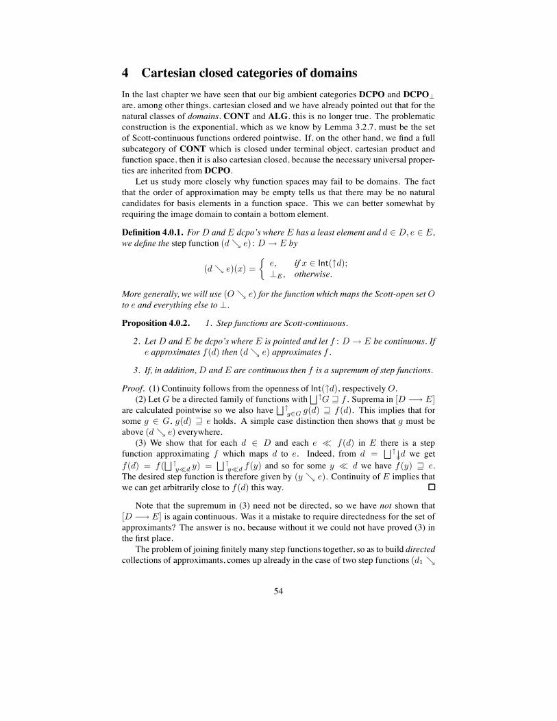
4 Cartesian closed categories of domainsIn the last chapter we have seen that our big ambient categories DCPO and DCPO$

are, among other things, cartesian closed and we have already pointed out that for thenatural classes of domains, CONT and ALG, this is no longer true. The problematicconstruction is the exponential, which as we know by Lemma 3.2.7, must be the setof Scott-continuous functions ordered pointwise. If, on the other hand, we find a fullsubcategory of CONT which is closed under terminal object, cartesian product andfunction space, then it is also cartesian closed, because the necessary universal proper-ties are inherited from DCPO.

Let us study more closely why function spaces may fail to be domains. The factthat the order of approximation may be empty tells us that there may be no naturalcandidates for basis elements in a function space. This we can better somewhat byrequiring the image domain to contain a bottom element.

Definition 4.0.1. For D and E dcpo’s where E has a least element and d ! D, e ! E,we define the step function (d E e) : D " E by

(d E e)(x) =

&

e, if x ! Int(/d);.E, otherwise.

More generally, we will use (O E e) for the function which maps the Scott-open setOto e and everything else to ..

Proposition 4.0.2. 1. Step functions are Scott-continuous.

2. Let D and E be dcpo’s where E is pointed and let f : D " E be continuous. Ife approximates f(d) then (d E e) approximates f .

3. If, in addition,D and E are continuous then f is a supremum of step functions.

Proof. (1) Continuity follows from the openness of Int(/d), respectivelyO.(2) LetG be a directed family of functions with

"

#G + f . Suprema in [D #" E]are calculated pointwise so we also have

"

#g"G g(d) + f(d). This implies that for

some g ! G, g(d) + e holds. A simple case distinction then shows that g must beabove (d E e) everywhere.

(3) We show that for each d ! D and each e : f(d) in E there is a stepfunction approximating f which maps d to e. Indeed, from d =

"

#00d we get

f(d) = f("

#y.d y) =

"

#y.d f(y) and so for some y : d we have f(y) + e.

The desired step function is therefore given by (y E e). Continuity of E implies thatwe can get arbitrarily close to f(d) this way.

Note that the supremum in (3) need not be directed, so we have not shown that[D #" E] is again continuous. Was it a mistake to require directedness for the set ofapproximants? The answer is no, because without it we could not have proved (3) inthe first place.

The problem of joining finitely many step functions together, so as to build directedcollections of approximants, comes up already in the case of two step functions (d1 E

54

D : E :

A B < f(A)

' d1

' d2 'f(d1) ' f(d2)'e1 ' e2

!!

!!

!!!"

""

""

"" !!

!!

!!

!!""

""

""

""!!

!! ""

""!!! "

"" !!! "

""!!! "

""""

""

Figure 10: Finding an upper bound for two step functions.

e1) and (d2 E e2) which approximate a given continuous function f . The situationis illustrated in Figure 10. The problem is where to map the (Scott-open but otherwiseunstructured) set A = //d1 * //d2. It has to be done in such a way that the resultingfunction still approximates f . As it will turn out, it suffices to make special assumptionsabout either the image domain E—the topic of Section 4.1— or about the pre-imagedomainD – the topic of Section 4.2. In both cases we restrict our attention to pointeddomains, and we work with step functions and joins of these. From these we can pass tomore general domains in again two ways. This will be outlined briefly in Section 4.3.2.The question then arises whether we have not missed out on some alternative way ofbuilding a cartesian closed category. This is not the case as we will see in Section 4.3.The basic tool for this fundamental result, Lemma 4.3.1, will nicely connect up withthe dichotomy distinguishing 4.1 and 4.2.

4.1 Local uniqueness: Lattice-like domainsThe idea for adjusting the image domain is simple; we assume that e1 and e2 have aleast upper bound e (if bounded at all). Mapping the intersection A to e (and //d1 \ Ato e1 and //d2 \ A to e2) results in a continuous function h which is above (d1 E e1)and (d2 E e2) and still approximates f . This is seen as follows: Suppose G is adirected collection of functions with supremum above f . Some g1 ! G must be above(d1 E e1) and some g2 ! G must be above (d2 E e2). Then by construction everyupper bound of {g1, g2} in G is above h.

In fact, we do not need that the join of e1 and e2 exists globally in E. It suffices toform the join for every a ! A inside 0f(a), because we have seen in Proposition 2.2.17that all considerations about the order of approximation can be performed inside prin-cipal ideals. We have the following list of definitions.

Definition 4.1.1. Let E be a pointed continuous domain. We say thatE is

1. an L-domain, if each pair e1, e2 ! E bounded by e ! E has a supremum in 0e;

2. a bounded-complete domain (or bc-domain), if each bounded pair e1, e2 ! Ehas a supremum;

55

' .X ! ALG \ L

'a ' b

'c1 ' c2

' =

!!!

""" !

!!

"""

//

//

//00

00

00

'C ! L \ BC

' '

' '

"""!

!!

//

//

//

00

00

00

'V ! BC \ LAT

' '!

!! """

Figure 11: Separating examples for the categories of lattice-like domains.

3. (repeated for comparison) a continuous lattice, if each pair e1, e2 ! E has asupremum.

We denote the full subcategories of CONT$ corresponding to these definitions byL, BC, and LAT. For the algebraic counterparts we use aL, aBC, and aLAT.

All this still makes sense if we forget about approximation but, surely, at this pointthe reader does not suffer from a lack of variety as far as categories are concerned.We would like to point out that continuous lattices are the main objects of study in[GHK+80], a mathematically oriented text, whereas the objects of "-aBC are oftenthe domains of choice in semantics, where they appear under the name Scott-domain.Typical examples are depicted in Figure 11. They even characterize the correspondingcategories, see Exercise 4.3.11(3).

Since domains have directed joins anyway, we see that in L-domains every subsetof a principal ideal has a supremum in that ideal. We also know that complete latticescan alternatively be characterized by infima. The same game can be played for theother two definitions:

Proposition 4.1.2. Let D be a pointed continuous domain. Then D is an L-domain, abc-domain, or a continuous lattice if and only if it has infima for bounded non-empty,non-empty, or arbitrary subsets, respectively.

The consideration of infima may seem a side issue in the light of the problem ofturning function spaces into domains. Its relevance becomes clear when we rememberthat upper adjoints preserve infima. The second half of the following is therefore asimple observation. The first half follows from Proposition 3.1.2 and Theorem 3.1.4.

Proposition 4.1.3. Retracts and bilimits of L-domains (bc-domains, continuous lat-tices) are again L-domains (bc-domains, continuous lattices).

We can treat continuous and algebraic lattice-like domains nicely in parallel be-cause the ideal completion respects these definitions:

56

Proposition 4.1.4. Let D be an L-domain (bc-domain, continuous lattice). ThenIdl(D,&) is an algebraic L-domain (bc-domain, lattice).

Thus L, BC, and LAT contain precisely the retracts of objects of aL, aBC, andaLAT, respectively. We conclude this section by stating the desired closure propertyof lattice-like domains.

Proposition 4.1.5. Let D be a continuous domain and E an L-domain (bc-domain,continuous lattice). Then [D #" E] is again an L-domain (bc-domain, continuouslattice).

Corollary 4.1.6. The categories L, BC, LAT, and their algebraic counterparts arecartesian closed.

4.2 Finite choice: Compact domainsLet us now turn our attention to the first argument of the function space construction,which means by the general considerations from the beginning of this chapter, the studyof open sets and their finite intersections. Step functions are defined using basic opensets of the form //d, and the fact that there is a single generator d was crucial in theproof that (d E e) approximates f whenever e approximates f(d). Arbitrary opensets are unions of such basic opens (Proposition 2.3.6) but in general this is an infiniteunion and so the proof of Proposition 4.0.2 will no longer work. For the first timewe have now reached a point in our exposition where the theory of algebraic domainsis definitely simpler and better understood than that of continuous domains. Let ustherefore treat this case first.

4.2.1 Bifinite domains

Step functions (d E e) may in the algebraic case be defined using compact elementsonly, where the characteristic pre-image //d is actually equal to /d. Taking up ourline of thought from above, we want for the algebraicity of the function space thatthe intersection A = /d1 * /d2 is itself generated by finitely many compact points:A = /c1 6 . . . 6 /cn. Note that the ci must be minimal upper bounds of {d1, d2}. Foreach ci we choose a compact element below f(ci) and above e1, e2. New intersectionsthen come up, this time between the different /ci’s. Let us therefore further assume thatafter finitely many iterations this process stops. It is an easy exercise to show that thefunction constructed in this way is a compact element below f and above (d1 E e1)and (d2 E e2). We hope that this provides sufficient motivation for the following listof definitions.

Definition 4.2.1. Let P be a poset. (Think of P as the basis of an algebraic domain.)

1. We say that P is mub-complete (or: has property m) if for every upper bound xof a finite subset M of P there is a minimal upper bound ofM below x. Writtenas a formula: >M 1fin P.

#

m"M /m = /mub(M).

2. For a subset A of P let its mub-closure mc(A) be the smallest superset of Awhich for every finiteM 1 mc(A) also containsmub(M).

57

3. We say that P has the finite mub property if it is mub-complete and if every finitesubset has a finite mub-closure. If, in addition, P has a least element, then wecall it a Plotkin-order.

4. An algebraic domain whose basis of compact elements is a Plotkin-order iscalled a bifinite domain. The full subcategory of ALG$ of bifinite domains wedenote by B.

With this terminology we can formulate precisely how finitely many step functionscombine to determine a compact element in the function space [Abr91b].

Definition 4.2.2. Let D be a bifinite domain and let E be pointed and algebraic. Afinite subset F of K(D) % K(E) is called joinable if

>G 1 F ?H 1 F. (*1(H) = mub(*1(G)) ' >c ! *2(G), d ! *2(H). c & d).

The function which we associate with a joinable family F is

x 9"$

{e | ?d ! K(D). d & x ' (d, e) ! F}.

Lemma 4.2.3. If D is a bifinite domain and E is pointed and algebraic, then everyjoinable subset of K(D) % K(E) gives rise to a compact element of [D #" E].

If F andG are joinable families then the corresponding functions are related if andonly if

>(d, e) ! G ?(d%, e%) ! F. d% & d and e & e%.

The expected result, dual to Proposition 4.1.5 above, then is:

Proposition 4.2.4. If D is a bifinite domain and E is pointed and algebraic, then[D #" E] is algebraic. All compact elements of [D #" E] arise from joinable fami-lies.

Comment: Proof sketch: Let f be a continuous function from D to E, and M be a finite mub-closedset of compact elements of D. Let (em)m#M be a collection of compact elements of E such thatfor all m " M , em # f(m). Then there exists a collection (em)m#M of compact elements of Esuch that the assignment m $% em is order-preserving. The new elements can be found by repeatedlyconsidering a minimal elementm ofM for which em has not yet been chosen, and by picking an upperbound for {em}& {em" | m$ < m}. With this construction one finds a directed collection of compactelements of [D '% E] arbitrarily close to f .

Note that this is strictly weaker than Proposition 4.1.5 and we do not immediatelyget that B is cartesian closed. For this we have to find alternative descriptions. Thefact that we can get an algebraic function space by making special assumptions abouteither the argument domain or the target domain was noted in a very restricted form in[Mar81].

The concept of finite mub closure is best explained by illustrating what can gowrong. In Figure 12 we have the three classical examples of algebraic domains whichare not bifinite; in the first one the basis is not mub-complete, in the second one there isan infinite mub-set for two compact elements, and in the third one, although all mub-sets are finite, there occurs an infinite mub-closure. On a more positive note, it is clear

58

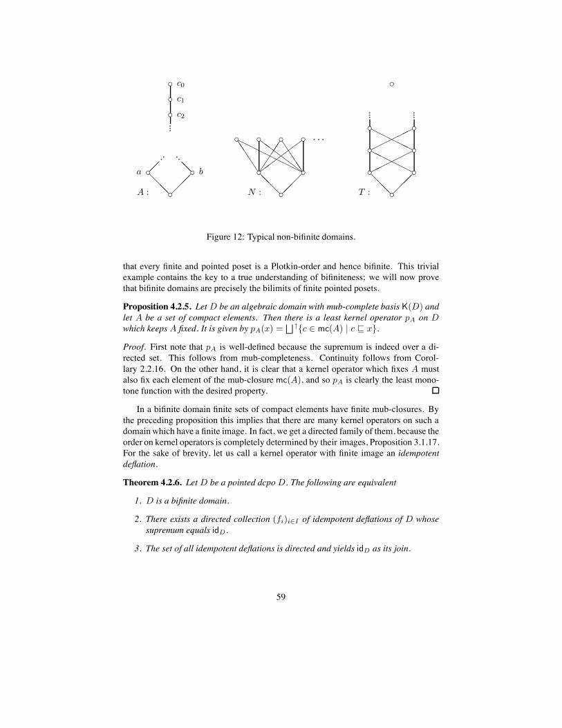
'A :

'a ' b

' c0

' c1

' c2

" " ""

"""

""!

!! """!!

'N :

' '

' ' ' ' " " "

"""!

!!8

888#######/

//

//

9999 8

888

00

000

'T :

' '' '' '

'

""" """

!!! "

""

#####))))) #####

)))))

Figure 12: Typical non-bifinite domains.

that every finite and pointed poset is a Plotkin-order and hence bifinite. This trivialexample contains the key to a true understanding of bifiniteness; we will now provethat bifinite domains are precisely the bilimits of finite pointed posets.

Proposition 4.2.5. Let D be an algebraic domain with mub-complete basis K(D) andlet A be a set of compact elements. Then there is a least kernel operator pA on Dwhich keeps A fixed. It is given by pA(x) =

"

#{c ! mc(A) | c & x}.

Proof. First note that pA is well-defined because the supremum is indeed over a di-rected set. This follows from mub-completeness. Continuity follows from Corol-lary 2.2.16. On the other hand, it is clear that a kernel operator which fixes A mustalso fix each element of the mub-closure mc(A), and so pA is clearly the least mono-tone function with the desired property.

In a bifinite domain finite sets of compact elements have finite mub-closures. Bythe preceding proposition this implies that there are many kernel operators on such adomainwhich have a finite image. In fact, we get a directed family of them, because theorder on kernel operators is completely determined by their images, Proposition 3.1.17.For the sake of brevity, let us call a kernel operator with finite image an idempotentdeflation.

Theorem 4.2.6. Let D be a pointed dcpoD. The following are equivalent

1. D is a bifinite domain.

2. There exists a directed collection (fi)i"I of idempotent deflations of D whosesupremum equals idD.

3. The set of all idempotent deflations is directed and yields idD as its join.

59

Proof. What we have not yet said is how algebraicity ofD follows from the existenceof idempotent deflations. For this observe that the inclusion of the image of a kerneloperator is a lower adjoint and as such preserves compactness. For the implication‘2 =( 3’ we use the fact that idempotent deflations are in any case compact elementsof the function space.

It is now only a little step to the promised categorical characterization.

Theorem 4.2.7. A dcpo is bifinite if and only if it is a bilimit of an expanding systemof finite pointed posets.

Proof. Let D be bifinite and let (fi)i"I be a family of idempotent deflations gener-ating the identity. Construct an expanding system by taking as objects the images ofthe deflations and as connecting embeddings the inclusion of images. The associatedupper adjoint is given by fi restricted to im(fj). D is the bilimit of this system byLemma 3.3.8.

If, conversely, ,D, (fi)i"I- is a bilimit of finite posets then clearly the compositionsfi 5 gi, where gi is the upper adjoint of fi, satisfy the requirements of Theorem 4.2.6.

So we have three characterizations of bifiniteness, the original one, which maybe called an internal description, a functional description by Theorem 4.2.6, and acategorical one by Theorem 4.2.7. Often, the functional characterization is the mosthandy one in proofs. We should also mention that bifinite domains were first definedby Gordon Plotkin in [Plo76] using expanding sequences. (In our taxonomy these areprecisely the countably based bifinite domains.) The acronym he used for them, SFP,continues to be quite popular.

Theorem 4.2.8. The category B of bifinite domains is closed under cartesian product,function space, coalesced sum, and bilimits. In particular, B is cartesian closed.

Proof. Only function space and bilimit are non-trivial. We leave the latter as an exer-cise. For the function space let D and E be bifinite with families of idempotent defla-tions (fi)i"I and (gj)j"J . A directed family of idempotent deflations on [D #" E] isgiven by the maps Fij : h 9" gj 5 h 5 fi, ,i, j- ! I % J .

4.2.2 FS-domains

Let us now look at continuous domains. The reasoning about what the structure of Dshould be in order to ensure that [D #" E] is continuous is pretty much the same asfor algebraic domains. But at the point where we there introduced the mub-closure ofa finite set of compact elements, we must now postulate the existence of some finiteand finitely supported partitioning of D. This is clearly an increase in the logicalcomplexity of our definition and also of doubtful practical use. It is more satisfactoryto generalise the functional characterization.

Definition 4.2.9. Let D be a dcpo and f : D " D be a Scott-continuous function.We say that f is finitely separated from the identity on D, if there exists a finite set M

60

such that for any x ! D there is m ! M with f(x) & m & x. We speak of strongseparation if for each x there are elements m, m% ! M with f(x) & m : m% & x.

A pointed dcpoD is called an FS-domain if there is a directed collection (fi)i"I ofcontinuous functions on D, each finitely separated from idD, with the identity map astheir supremum.

It is relatively easy to see that FS-domains are indeed continuous. Thus it makessense to speak of FS as the full subcategory of CONT where the objects are the FS-domains.

We have exact parallels to the properties of bifinite domains, but often the proofsare trickier.

Proposition 4.2.10. If D is an FS-domain and E is pointed and continuous then[D #" E] is continuous.

Comment: Unfortunately, the proof of this is not only “trickier” but as yet unknown. What is true,is that when both D and E are FS-domains, then [D '% E] is also an FS-domains. This was shownin [Jun90]. The following theorem is therefore still valid.

Theorem 4.2.11. The category FS is closed under the formation of products, functionspaces, coalesced sums, and bilimits. It is cartesian closed.

What we do not have are a categorical characterization or a description of FS-domains as retracts of bifinite domains. All we can say is the following.

Proposition 4.2.12. 1. Every bifinite domain is an FS-domain.

2. A retract of an FS-domain is an FS-domain.

3. An algebraic FS-domain is bifinite.

To fully expose our ignorance, we conclude this subsection with an example of awell-structured FS-domain of which we do not know whether it is a retract of a bifinitedomain.Example. Let Disc be the collection of all closed discs in the plane plus the plane

itself, ordered by reversed inclusion. One checks that the filtered intersection of discsis again a disc, so Disc is a pointed dcpo. A disc d1 approximates a disc d2 if and onlyif d1 is a neighborhood of d2. This proves that Disc is continuous. For every ' > 0we define a map f" on Disc as follows. All discs inside the open disc with radius 1

"are

mapped to their closed '-neighborhood, all other discs are mapped to the plane whichis the bottom element of Disc. Because the closed discs contained in some compactset form a compact space under the Hausdorff subspace topology, these functions arefinitely separated from the identity map. This proves that Disc is a countably basedFS-domain.

4.2.3 Coherence

This is a good opportunity to continue our exposition of the topological side of domaintheory, which we began in Section 2.3. We need a second tool complementing the

61

lattice )D of Scott-open sets, namely, the compact saturated sets. Here ‘compact’ is tobe understood in the classical topological sense of the word, i.e. a setA of a topologicalspace is compact if every covering of A by open sets contains a finite subcovering.Saturated are those sets which are intersections of their neighborhoods. In dcpo’sequipped with the Scott-topology these are precisely the upper sets, as is easily seenusing opens of the formD \ 0x.

Theorem 4.2.13. Let D be a continuous domain. The sets of open neighborhoods ofcompact saturated sets are precisely the Scott-open filters in )D .

By Proposition 7.2.27 this is a special case of the Hofmann-MisloveTheorem 7.2.9.Let us denote the set of compact saturated sets of a dcpo D, ordered by reverse

inclusion, by +D. We will refer to families in +D which are directed with respect toreverse inclusion, more concretely as filtered families. The following, then, is only are-formulation of Corollary 7.2.11.

Proposition 4.2.14. Let D be a continuous domain.

1. +D is a dcpo. Directed suprema are given by intersection.

2. If the intersection of a filtered family of compact saturated sets is contained in aScott-open set O then some element of it belongs to O already.

3. +D \ {B} is a dcpo.

Proposition 4.2.15. Let D be a continuous domain.

1. +D is a continuous domain.

2. A : B holds in +D if and only if there is a Scott-open set O with B 1 O 1 A.

3. O : U holds in )D if and only if there is a compact saturated set A withO 1 A 1 U .

Proof. All three claims are shown easily using upper sets generated by finitely manypoints: If O is an open neighborhood of a compact saturated set A then there exists afinite setM of points of O with A 1 //M 1 /M 1 O.

The interesting point about FS-domains then is, that their space of compact sat-urated sets is actually a continuous lattice. We already have directed suprema (inthe form of filtered intersections) and continuity, so this boils down to the propertythat the intersection of two compact saturated sets is again compact. Let us call do-mains for which this is true, coherent domains. Given the intimate connection between)D and +D , it is no surprise that we can read off coherence from the lattice of opensets.

Proposition 4.2.16. A continuous domain D is coherent if and only if for allO, U1, U2 ! )D with O : U1 and O : U2 we also have O : U1 * U2.

(In Figure 6 we gave an example showing that the condition is not true in arbitrarycontinuous lattices.)

This result specializes for algebraic domains as follows:

62

Proposition 4.2.17. An algebraic domain D is coherent if and only if K(D) is mub-complete and finite sets of K(D) have finite sets of minimal upper bounds.

This proposition was named ‘2/3-SFP Theorem’ in [Plo81] because coherencerules out precisely the first two non-examples of Plotkin-orders, Figure 12, but notthe third. The only topological characterization of bifinite domains we have at themoment, makes use of the continuous function space, see Lemma 4.3.2.

We observe that for algebraic coherent domains, )D and +D have a common sub-lattice, namely that of compact-open sets. These are precisely the sets of the form/c1 6 . . . 6 /cn with the ci compact elements. This lattice generates both )D and +D

when we form arbitrary suprema. This pleasant coincidence features prominently inChapter 7.

Theorem 4.2.18. FS-domains (bifinite domains) are coherent.

Let us reformulate the idea of coherence in yet another way.

Definition 4.2.19. The Lawson-topology on a dcpo D is the smallest topology con-taining all Scott-open sets and all sets of the formD \ /x. It is denoted by !D.

Proposition 4.2.20. Let D be a continuous domain.

1. The Lawson-topology on D is Hausdorff. Every Lawson-open set has the formO \ A where O is Scott-open and A is Scott-compact saturated.

2. The Lawson-topology on D is compact if and only if D is coherent.

3. A Scott-continuous retract of a Lawson-compact continuous domain is Lawson-compact and continuous.

So we see that FS-domains and bifinite domains carry a natural compact Hausdorfftopology. We will make use of this in Chapter 6.

4.3 The hierarchy of categories of domainsThe purpose of this section is to show that there are no other ways of constructing acartesian closed full subcategory ofCONT orALG than those exhibited in the previoustwo sections. The idea that such a result could hold originated with Gordon Plotkin,[Plo81]. For the particular class "-ALG$ it was verified by Mike Smyth in [Smy83a],for the other classes by Achim Jung in [Jun88, Jun89, Jun90]. All these classificationresults depend on the Axiom of Choice.

4.3.1 Domains with least element

Let us start right away with the crucial bifurcation lemma on which everything else inthis section is based.

Lemma 4.3.1. Let D and E be continuous domains, where E is pointed, such that[D #" E] is continuous. ThenD is coherent or E is an L-domain.

63

Proof. By contradiction. Assume D is not coherent and E is not an L-domain. ByProposition 4.2.16 there exist open sets O, U1, and U2 in D such that O : U1 andO : U2 hold but notO : U1 *U2. Therefore there is a directed collection (Vi)i"I ofopen sets covering U1 * U2, none of which covers O. We shall also need interpolatingsets U %

1 and U %2, that is, O : U %

1 : U1 and O : U %2 : U2.

The assumption aboutE not being an L-domain can be transformed into two specialcases. EitherE contains the algebraic domainA from Figure 12 (where the descendingchain in A may generally be an ordinal) or X from Figure 11 as a retract. We have leftthe proof of this as Exercise 4.3.11(3). Note that if E% is a retract of E then [D #" E%]is a retract of [D #" E] and hence the former is continuous if the latter is. Let us nowprove for both cases that [D #" E] is not continuous.

Case 1: E = A. Consider the step functions f1 = (U %1 E a) and f2 = (U %

2 E b).They clearly approximate f , which is defined by

f(x) =

)

*

*

+

*

*

,

c0, if x ! U1 * U2;a, if x ! U1 \ U2;b, if x ! U2 \ U1;., otherwise.

Since approximating sets are directed we ought to find an upper bound g for f1 and f2

approximating f . But this impossible: Given an upper bound of {f1, f2} below f wehave the directed collection (hi)i"I defined by

hi(x) =

)

+

,

c0, if x ! Vi;cn+1, if x ! (U1 * U2) \ Vi and g(x) = cn;g(x), otherwise.

No hi is above g because (U1*U2)\Vi must contain a non-empty piece ofO and therehi is strictly below g. The supremum of the hi, however, equals f . Contradiction.

Case 2: E = X . We choose open sets in D as in the previous case. The variousfunctions, giving the contradiction, are now defined by f1 = (U %

1 E a), f2 = (U %2 E

b),

f(x) =

)

*

*

+

*

*

,

c1, if x ! U1 * U2;a, if x ! U1 \ U2;b, if x ! U2 \ U1;., otherwise.

hi(x) =

)

+

,

=, if x ! Vi;c2, if x ! (U1 * U2) \ Vi;g(x), otherwise.

The remaining problem is that coherence does not imply that D is an FS-domain(nor, in the algebraic case, that it is bifinite). It is taken care of by passing to higher-order function spaces:

Lemma 4.3.2. Let D be a continuous domain with bottom element. Then D is anFS-domain if and only if both D and [D #" D] are coherent.

64

(The proof may be found in [Jun90].)Combining the preceding two lemmas with Lemmas 3.2.5 and 3.2.7 we get the

promised classification result.

Theorem 4.3.3. Every cartesian closed full subcategory of CONT$ is contained inFS or L.

Adding Proposition 4.2.12 we get the analogue for algebraic domains:

Theorem 4.3.4. Every cartesian closed full subcategory of ALG$ is contained in Bor aL.

Forming the function space of an L-domain may in general increase the cardinalityof the basis (Exercise 4.3.11(17)). If we restrict the cardinality, this case is ruled out:

Theorem 4.3.5. Every cartesian closed full subcategory of "-CONT$ ("-ALG$) iscontained in "-FS ("-B).

4.3.2 Domains without least element

The classification of pointed domains, as we have just seen, is governed by the di-chotomy between coherent and lattice-like structures. Expressed at the element level,and at least for algebraic domains we have given the necessary information, it is thedistinction between finite mub-closures and locally unique suprema of finite sets. Itturns out that passing to domains which do not necessarily have bottom elements im-plies that we also have to study the mub-closure of the empty set. We get again thesame dichotomy. Coherence in this case means that D itself, that is, the largest ele-ment of )D, is a compact element. This is just the compactness of D as a topologicalspace. And the property that E is lattice-like boils down to the requirement that eachelement of E is above a unique minimal element, so E is really the disjoint union ofpointed components.

Lemma 4.3.6. LetD andE be continuous domains such that [D #" E] is continuous.Then D is compact or E is a disjoint union of pointed domains.

The proof is a cut-down version of that of Lemma 4.3.1 above. The surprisingfact is that this choice can be made independently from the choice between coher-ent domains and L-domains. Before we state the classification, which because of thisindependence, will now involve 2 % 2 = 4 cases, we have to refine the notion of com-pactness, because just like coherence it is not the full condition necessary for cartesianclosure.

Definition 4.3.7. A dcpoD is a finite amalgam if it is the union of finitely many pointeddcpo’sD1, . . . , Dn such that every intersection of Di’s is also a union of Di’s. (Com-pare the definition of mub-complete.)

For categories whose objects are finite amalgams of objects from another cate-gory C we use the notation F-C. Similarly, we write U-C if the objects are disjointunions of objects of C.

65

Proposition 4.3.8. A mub-complete dcpo is a finite amalgam if and only if the mub-closure of the empty set is finite.

Lemma 4.3.9. If bothD and [D #" D] are compact and continuous thenD is a finiteamalgam.

Theorem 4.3.10. 1. The maximal cartesian closed full subcategories ofCONT areF-FS, U-FS, F-L, and U-L.

2. The maximal cartesian closed full subcategories of ALG are F-B, U-B, F-aL,and U-aL.

At this point we can answer a question that may have occurred to the diligent readersome time ago, namely, why we have defined bifinite domains in terms of pointed finiteposets, where clearly we never needed the bottom element in the characterizations ofthem. The answer is that we wanted to emphasize the uniform way of passing frompointed to general domains. The fact that the objects of F-B can be represented asbilimits of finite posets is then just a pleasant coincidence.

Exercises 4.3.11. 1. [Jun89] Show that a dcpo D is continuous if the functionspace [D #" D] is continuous.

2. LetD be a bounded-complete domain. Show that ‘3’ is a Scott-continuous func-tion from D % D to D.

3. Characterize the lattice-like (pointed) domains by forbidden substructures:

(a) E is "-continuous but not mub-complete if and only if domain A in Fig-ure 12 is a retract of E.

(b) E is mub-complete but not an L-domain if and only if domain X in Fig-ure 11 is a retract of E.

(c) E is an L-domain but not bounded-complete if and only if domain C inFigure 11 is a retract of E.

(d) E is a bounded-complete domain but not a lattice if and only if domain Vin Figure 11 is a retract of E.

4. Find a poset in which all pairs have finite mub-closures but in which a triple ofpoints exists with infinite mub-closure.

5. Show that if for an algebraic domain D the basis is mub-complete then D itselfis not necessarily mub-complete.

6. Show that in a bifinite domain finite sets of non-compact elements may haveinfinitely many minimal upper bounds and, even if these are all finite, may haveinfinite mub-closures.

7. Show that if A is a two-element subset of an L-domain then A 6 mub(A) ismub-closed.

8. Prove that bilimits of bifinite domains are bifinite.

66

9. Prove the following statements about retracts of bifinite domains.

(a) A pointed dcpo D is a retract of a bifinite domain if and only if there is adirected family (fi)i"I of functions on D such that each fi has a finite im-age and such that

"

#i"I fi = idD. (You may want to do this for countably

based domains first.)(b) The ideal completion of a retract of a bifinite domain need not be bifinite.(c) If D is a countably based retract of a bifinite domain then it is also the

image of a projection from a bifinite domain. (Without countability this isan open problem.)

(d) The category of retracts of bifinite domains is cartesian closed and closedunder bilimits.

10. Prove that FS-domains have infima for downward directed sets. As a conse-quence, an FS-domain which has binary infima, is a bc-domain.

11. Show that in a continuous domain the Lawson-closed upper sets are preciselythe Scott-compact saturated sets.

12. Characterize Lawson-continuous maps between bifinite domains.

13. We have seen that every bifinite domain is the bilimit of finite posets. As such,it can be thought of as a subset of the product of all these finite posets. Provethat the Lawson-topology on the bifinite domain is the restriction of the producttopology if each finite poset is equipped with the discrete topology.

14. Prove that a coherent L-domain is an FS-domain.

15. Characterize those domains which are both L-domains and FS-domains.

16. Characterize Scott-topology and Lawson-topology on both L-domains and FS-domains by the ideal of functions approximating the identity.

17. [Jun89] Let E be an L-domain such that [E #" E] is countably based. Showthat E is an FS-domain.

67

5 Recursive domain equationsThe study of recursive domain equations is not easily motivated by reference to othermathematical structure theories. So we shall allow ourselves to deviate from our gen-eral philosophy and spend some time on examples. Beyond motivation, our examplesrepresent three different (and almost disjoint) areas in which recursive domain equa-tions arise, in which they serve a particular role, and in which particular aspects aboutsolutions become prominent. It is an astonishing fact that within domain theory allthese aspects are dealt with in a unified and indeed very satisfactory manner. This rich-ness and interconnectedness of the theory of recursive domain equations, beautiful as itis, may nevertheless appear quite confusing on a first encounter. As a general guidelinewe offer the following: Recursive domain equations and the domain theory for solv-ing them comprise a technique that is worth learning. But in order to understand themeaning of a particular recursive domain equation, you have to know the context inwhich it came up.

5.1 Examples5.1.1 Genuine equations

The prime example here is X $= [X #" X ]. Solving this equation in a cartesianclosed category gives a model for the untyped !-calculus [Sco80, Bar84], in which, aswe know, no type distinction is made between functions and arguments. When settingup an interpretation of !-terms with values in D, where D solves this equation, weneed the isomorphisms % : D " [D #" D] and , : [D #" D] " D explicitly. Weconclude that even in the case of a genuine equation we are looking not only for anobject but an object plus an isomorphism. This is a first hint that we shall need totreat recursive domain equations in a categorical setting. However, the function spaceoperator is contravariant in its first and covariant in its second argument and so thereis definitely an obstacle to overcome. A second problem that this example illustratesis that there may be many solutions to choose from. How do we recognize a canonicalone? This will be the topic of Section 5.3.

Besides this classical example, genuine equations are rare. They come up in se-mantics when one is confronted with the ability of computers to treat information bothas program text and as data.

5.1.2 Recursive definitions

In semantics we sometimes need to make recursive definitions, for very much the samereasons that we need recursive function calls, namely, we sometimes do not know howoften the body of a definition (resp. function) needs to be repeated. To give an example,take the following definition of a space of so-called ‘resumptions’:

R $= [S #" (S C S % R)].

We read it as follows: A resumption is a map which assigns to a state either a final stateor an intermediary state together with another resumption representing the remaining

68

computation. Such a recursive definition is therefore nothing but a shorthand for aninfinite (but regular) expression. Likewise, awhile loop could be replaced by an infiniterepetition of its body. This analogy suggests that the way to give meaning to a recursivedefinition is to seek a limit of the repeated unwinding of the body of the definitionstarting from a trivial domain. No doubt this is in accordance with our intuition, andindeed this is how we shall solve equations in general. But again, before we can dothis, we need to be able to turn the right hand side of the specification into a functor.

5.1.3 Data types

Data types are algebras, i.e. sets together with operations. The study of this notion isknown as ‘Algebraic Specification’ [EM85] or ‘Initial Algebra Semantics’ [GTW78].We choose a formulation which fits nicely into our general framework.

Definition 5.1.1. Let F be a functor on a categoryC. An F -algebra is given by an ob-ject A and a map f : F (A) " A. A homomorphism between algebras f : F (A) " Aand f % : F (A%) " A% is a map g : A " A% such that the following diagram commutes:

F (A)F (g)& F (A%)

A

f

' g & A%

f %

'

For example, if we let F be the functor over Set which assigns I.6 A % A to A

(where I is the one-point dcpo as discussed in Section 3.2.1), then F -algebras are pre-cisely the algebras with one nullary and one binary operation in the sense of universalalgebra. Lehmann and Smyth [LS81] discuss many examples. Many of the data typeswhich programming languages deal with are furthermore totally free algebras, or termalgebras on no generators. These are distinguished by the fact that there is preciselyone homomorphism from them into any other algebra of the same signature. In our cat-egorical language we express this by initiality. Term algebras (alias initial F -algebras)are connected with the topic of this chapter because of the following observation:

Lemma 5.1.2. If i : F (A) " A is an initial F -algebra then i is an isomorphism.

Proof. Consider the following composition of homomorphisms:

F (A)F (f)& F 2(A)

F (i)& F (A)

A

i

' f & F (A)

F (i)

' i & A

i

'

where f is the unique homomorphism from i : F (A) " A to F (i) : F 2(A) " F (A)guaranteed by initiality. Again by initiality, i 5 f must be idA. And from the first

69

quadrangle we get f 5 i = F (i) 5 F (f) = F (idA) = idF (A). So f and i are inversesof each other.

So in order to find an initial F -algebra, we need to solve the equationX $= F (X).But once we get a solution, we still have to check initiality, that is, we must validatethat the isomorphism from F (X) to X is the right structure map.

In category theory we habitually dualize all definitions. In this case we get (final)co-algebras. Luckily, this concept is equally meaningful. Where the map f : F (A) "A describes the way how new objects of type A are constructed from old ones, a mapg : A " F (A) stands for the opposite process, the decomposition of an object into itsconstituents. Naturally, we want the two operations to be inverses of each other. Inother words, if i : F (A) " A is an initial F -algebra, then we require i&1 : A " F (A)to be the final co-algebra.

Peter Freyd [Fre91] makes this reasoning the basis of an axiomatic treatment ofdomain theory. Beyond and above axiomatizing known results, he treats contravariantand mixed variant functors and offers a universal property encompassing both initial-ity and finality. This will allow us to judge the solution of general recursive domainequations with respect to canonicity.

5.2 Construction of solutionsSuppose we are given a recursive domain equation X $= F (X) where the right handside defines a functor on a suitable category of domains. As suggested by the ex-ample in Section 5.1.2, we want to repeat the trick which gave us fixpoints for Scott-continuous functions, namely, to take a (bi-)limit of the sequence I, F (I), F (F (I)), . . . .Remember that bilimits are defined in terms of e-p-pairs. This makes it necessary thatwe, at least temporarily, switch to a different category. The convention that we adoptfor this chapter is to let D stand for any category of pointed domains, closed underbilimits. All the cartesian closed categories of pointed domains mentioned in Chapter 4qualify. We denote the corresponding subcategory where the morphisms are embed-dings by De. Some results will only hold for strict functions. Recall that our notationfor these were f : D

$!#" E andD$! for categories. Despite this unhappy (but unavoid-

able) proliferation of categories, recall that the central limit-colimit Theorem 3.3.7 andCorollary 3.3.10 state a close connection: Colimits of expanding sequences in De arealso colimits in D and, furthermore, if the embeddings defining the sequence are re-placed by their upper adjoints, the colimit coincides with the corresponding limit. Thiswill bear fruit when we analyze the solutions we get in De from various angles assuggested by the examples in the last subsection.

Let us now start by just assuming that our functor restricts to De.

5.2.1 Continuous functors

Definition 5.2.1. A functor F : De " De is called continuous, if for every ex-panding sequence ,(Dn)n"N, (emn : Dn " Dm)n/m"N- with colimit ,D, (en)n"N-we have that ,F (D), (F (en))n"N- is a colimit of the sequence ,(F (Dn))n"N,(F (emn) : F (Dn) " F (Dm))n/m"N-.

70

This, obviously, is Scott-continuity expressed for functors. Whether we formulateit in terms of expanding sequences or expanding systems is immaterial. The question isnot, what is allowed to enter the model, but rather, how much do I have to check beforeI can apply the theorems in this chapter. And sequences are all that is needed.

This, then, is the central lemma on which our domain theoretic technique for solv-ing recursive domain equations is based (recall that f( is our notation for the upperadjoint of f ):

Lemma 5.2.2. Let F be a continuous functor on a category De of domains. For eachembedding e : A " F (A) consider the colimit ,D, (en)n"N- of the expanding se-quence A

e#" F (A)

F (e)#" F (F (A))

F (F (e))#" · · · . Then D is isomorphic to F (D) via

the maps

fold ="

#n"N

en+1 5 F (en)( : F (D) " D, andunfold =

"

#n"N

F (en) 5 e(n+1 : D " F (D).

For each n ! N they satisfy the equations

F (en) = unfold 5 en+1

F (en)( = e(n+1 5 fold .

Proof. We know that ,D, (en)n"N\{0}- is a colimit over the diagram

F (A)F (e)#" F (F (A))

F (F (e))#" · · ·

(clipping off the first approximation makes no difference), where there is also the co-cone ,F (D), (F (en))n"N-. The latter is also colimiting by the continuity of F . Inthis situation Theorem 3.3.7 provides us with unique mediating morphisms which areprecisely the stated fold and unfold. They are inverses of each other because both co-cones are colimiting. The equations follow from the explicit description of mediatingmorphisms in Theorem 3.3.7.

Note that since we have restricted attention to pointed domains, we always have theinitial embedding e : I " F (I). The solution to X $= F (X) based on this embeddingwe call canonical and denote it by FIX(F ).

5.2.2 Local continuity

Continuity of a functor is a hard condition to verify. Luckily there is a property whichis stronger but nevertheless much easier to check. It will also prove useful in the nextsection.

Definition 5.2.3. A functor F from D to E, where D and E are categories of domains,is called locally continuous, if the maps Hom(D, D%) #" Hom(F (D), F (D%)), f 9"F (f), are continuous for all objectsD andD% from D.

Proposition 5.2.4. A locally continuous functor F : D " E restricts to a continuousfunctor from De to Ee.

71

We will soon generalize this, so there is no need for a proof at this point.Typically, recursive domain equations are built from the basic constructions listed

in Section 3.2. The strategy is to check local continuity for each of these individuallyand then rely on the fact that composition of continuous functors yields a continuousfunctor. However, we must realize that the function space construction is contravariantin its first and covariant in its second variable, and so the technique from the precedingparagraph does not immediately apply. Luckily, it can be strengthened to cover thiscase as well.

Definition 5.2.5. A functor F : Dop % D’ " E, contravariant in its first, covariant inits second variable, is called locally continuous, if for directed setsA 1 Hom(D2, D1)andA% 1 Hom(D%

1, D%2) (whereD1, D2 are objects inD andD%

1, D%2 are objects inD’)

we haveF (

$

#A,$

#A%) =$

#

f"A,f ""A"

F (f, f %)

in Hom(F (D1, D%1), F (D2, D%

2)).

Proposition 5.2.6. If F : Dop % D’" E is a mixed variant, locally continuous functor,then it defines a continuous covariant functor F from De % D’e to Ee as follows:

F (D, D%) = F (D, D%) for objects, andF (e, e%) = F (e(, e%) for embeddings.

The upper adjoint to F (e, e%) is given by F (e, e%().

Proof. Let (e, e() and (e%, e%() be e-p-pairs in D and D’, respectively. We calculateF (e, e%() 5 F (e, e%) = F (e, e%() 5 F (e(, e%) = F (e( 5 e, e%( 5 e%) = F (id, id) = id andF (e, e%) 5 F (e, e%() = F (e(, e%) 5 F (e, e%() = F (e 5 e(, e% 5 e%() & F (id, id) = id, soF maps indeed pairs of embeddings to embeddings.

For continuity, let ,(Dn), (emn)- and ,(D%n), (e%mn)- be expanding sequences in

D and D’ with colimits ,D, (en)- and ,D%, (e%n)-, respectively. By Lemma 3.3.8this implies

"

#n"N

en 5 e(n = idD and"

#n"N

e%n 5 e%(n = idD" . By lo-cal continuity we have

"

#n"N

F (en, e%n) 5 F (en, e%n)( ="

#n"N

F (e(n, e%n) 5F (en, e%(n) =

"

#n"N

F (en 5 e(n, e%n 5 e%(n) = F ("

#n"N

en 5 e(n,"

#n"N

e%n 5 e%(n) =

F (idD, idD") = idF (D,D") and so ,F (D, D%), (F (en, e%n))n"N- is a colimit of,(F (Dn, D%

n))n"N, (F (emn, e%mn))n/m"N-.

While it may seem harmless to restrict a covariant functor to embeddings in orderto solve a recursive domain equation, it is nevertheless not clear what the philosophicaljustification for this step is. For mixed variant functors this question becomes evenmore pressing since we explicitly change the functor. As already mentioned, a satis-factory answer has only recently been found, [Fre91, Pit93b]. We present Peter Freyd’ssolution in the next section.

Let us take stock of what we have achieved so far. Building blocks for recursivedomain equations are the constructors of Section 3.2, %,C,", etc. , each of which isreadily seen to define a locally continuous functor. Translating them to embeddings

72

via the preceding proposition, we get continuous functors of one or two variables. Wefurther need the diagonal ! : De " De % De to deal with multiple occurrences ofX in the body of the equation. Then we note that colimits in a finite power of De

are calculated coordinatewise and hence the diagonal and the tupling of continuousfunctors are continuous. Finally, we include constant functors to allow for constants tooccur in an equation. Two more operators will be added below: the bilimit in the nextsection and various powerdomain constructions in Chapter 6.

5.2.3 Parameterized equations

Suppose that we are given a locally continuous functor F in two variables. Givenany domain D we can solve the equation X $= F (D, X) using the techniques ofthe preceding sections. Remember that by default we mean the solution accordingto Lemma 5.2.2 based on e : I " F (D, I), so there is no ambiguity. Also, we havegiven a concrete representation for bilimits in Theorem 3.3.7, so FIX(F (D, ·)) is alsowell-defined in this respect. We want to show that it extends to a functor.

Notation is a bit of a problem. Let F : D$! % E$! " E$! be a functor in twovariables. We set FD for the functor on E$! which maps E to F (D, E) for objects andg : E

$!#" E% to F (idD, g) for morphisms. Similarly for FD" . The embeddings into the

canonical fixpoint of FD , resp. FD" , we denote by e0, e1, . . . and e%0, e%1, . . . , and we

use e and e% for the unique strict function from I intoD andD%, respectively.

Proposition 5.2.7. Let F : D$! % E$! " E$! be a locally continuous functor. Thenthe following defines a locally continuous functor from D$! to E$!:

On objects : D 9" FIX(FD),

on morphisms : (f : D " D%) 9"$

#

n"N

e%n 5 fn 5 e(n

where the sequence (fn)n"N is defined recursively by f0 = idI, fn+1 = F (f, fn).

Proof. Let D and D% be objects of D$! and let f : D$!#" D% be a strict function. The

solution toX $= F (D, X) is given by the bilimit

FIX(FD)

""

""

e0

: ;!!

!!

e2 . . .

Ie& FD(I)

e1

<

FD(e)& F 2D(I) & · · ·

and similarly for D%. Corresponding objects of the two expanding sequences are con-nected by fn : Fn

D(I) $!#" Fn

D"(I). They commute with the embeddings of the expand-ing sequences: For n = 0 we have F 0

D"(e%) 5 f0 = e% 5 idI = e% = f1 5 e = f1 5 F 0D(e)

because there is only one strict map from I to F 1(D%). Higher indices follow by induc-

73

tion:

Fn+1D" (e%) 5 fn+1 = F (idD" , Fn

D"(e%)) 5 F (f, fn)

= F (f, FnD"(e%) 5 fn)

= F (f, fn+1 5 FnD(e))

= F (f, fn+1) 5 F (idD, FnD(e))

= fn+2 5 Fn+1D (e).

So we have a second cocone over the sequence defining FIX(FD) and using the factthat colimits in E$!

e are also colimits in E$!, we get a (unique) mediating morphismfrom FIX(FD) to FIX(FD"). By Theorem 3.3.7 it has the postulated representation.

Functoriality comes for free from the uniqueness of mediating morphisms. It re-mains to check local continuity. So let A be a directed set of maps from D to D%. Weeasily get (

"

#A)n ="

#f"A fn by induction and the local continuity of F . The supre-

mum can be brought to the very front by the continuity of composition and generalassociativity.

Note that this proof works just as well for mixed variant functors. As an application,suppose we are given a system of simultaneous equations

X1$= F1(X1, . . . , Xn)

......

Xn$= Fn(X1, . . . , Xn).

We can solve these one after the other, viewing X2, . . . , Xn as parameters for thefirst equation, substituting the result for X1 in the second equation and so on. It ismore direct to pass from D to Dn, for which Theorem 3.3.7 and the results of thischapter remain true, and then solve these equations simultaneously with the tupling ofthe Fi. The fact that these two methods yield isomorphic results is known as Bekic’srule [Bek69].

5.3 CanonicityWe have seen in the first section of this chapter that recursive domain equations arisein various contexts. After having demonstrated a technique for solving them, we mustnow check whether the solutions match the particular requirements of these applica-tions.

5.3.1 Invariance and minimality

Let us begin with a technique of internalizing the expanding sequence I " F (I) "F (F (I)) " · · · into the canonical solution. This will allow us to do proofs aboutFIX(F ) without (explicit) use of the defining expanding sequence.

Lemma 5.3.1. Let F be a locally continuous functor on a category of domains D andlet i : F (A) " A be an isomorphism. Then there exists a least homomorphism hC,A

74

from A to every other F -algebra f : F (C) " C. It equals the least fixpoint of thefunctional %C,A on [A #" C] which is defined by

%C,A(g) = f 5 F (g) 5 i&1 .

Least homomorphisms compose: If j : F (B) " B is also an isomorphism, thenhC,A = hC,B 5 hB,A.

Proof. The functional % = %C,A is clearly continuous because F is locally continu-ous and composition is a continuous operation. Since we have globally assumed leastelements, the function space [A #" C] contains c$ as a least element. So the leastfixpoint hC,A of %C,A calculated as the supremum of the chain c$ & %(c$) & · · ·exists. We show by induction that it is below every homomorphism h. For c$ this isobvious. For the induction step assume g & h. We calculate: %(g) = f 5F (g) 5 i&1 &f 5F (h) 5 i&1 = h. It follows that fix(%) = hC,A & h holds. On the other hand, everyfixpoint of % is a homomorphism: h 5 i = %(h) 5 i = f 5 F (h) 5 i&1 5 i = f 5 F (h).

The claim about composition of least homomorphisms can also be shown by in-duction. But it is somewhat more elegant to use the invariance of least fixpoints,Lemma 2.1.21. Consider the diagram

[B #" C]H& [A #" C]

[B #" C]

%C,B

' H& [A #" C]

%C,A

'

whereH is the strict operation which assigns g 5hB,A to g ! [B #" C]. The diagramcommutes, because H 5 %C,B(g) = f 5 F (g) 5 j&1 5 hB,A = f 5 F (g 5 hB,A) 5 i&1

(because hB,A is an homomorphism) = %C,A(H(g)). Lemma 2.1.21 then gives usthe desired equality: hC,A = fix(%C,A) = H(fix(%C,B)) = fix(%C,B) 5 hB,A =hC,B 5 hB,A.

Specializing the second algebra in this lemma to be i : F (A) " A itself, we de-duce that on every fixpoint of a locally continuous functor there exists a least endomor-phism hA,A. Since the identity is always an endomorphism, the least endomorphismmust be below the identity and idempotent, i.e. a kernel operator and in particular strict.This we will use frequently below.

Theorem 5.3.2. (Invariance, Part 1) Let F be a locally continuous functor on a cate-gory of domains D and let i : F (A) " A be an isomorphism. Then the following areequivalent:

1. A is isomorphic to the canonical fixpoint FIX(F );

2. idA is the least endomorphism of A;

3. idA = fix(%A,A) where %A,A : [A #" A] " [A #" A] is defined by %A,A(g) =i 5 F (g) 5 i&1;

75

4. idA is the only strict endomorphism of A.

Proof. (1=( 2) The least endomorphism on D = FIX(F ) is calculated as the leastfixpoint of %D,D : g 9" fold5F (g)5unfold. With the usual notation for the embeddingsof Fn(I) into D we get (by induction): c$ = e0 5 e(0 and %n(c$) = %(%n&1(c$)) =%(en&1 5e(n&1) = fold5F (en&1)5F (e(n&1)5unfold = en 5e(n, where the last equalityfollows because fold and unfold are mediating morphisms. Lemma 3.3.8 entails thatthe supremum of the %n(c$) is the identity.

The equivalence of (2) and (3) is a reformulation of Lemma 5.3.1.(3=( 4) Suppose h : A

$!#" A defines an endomorphism of the algebra

i : F (A) " A. We apply the invariance property of least fixpoints, Lemma 2.1.21,to the diagram (where % now stands for %A,A)

[A #" A]H& [A #" A]

[A #" A]

%

' H& [A #" A]

%

'

whereH maps g ! [A #" A] to h5g. This is a strict operation because h is assumed tobe strict. The diagram commutes: H 5%(g) = H(i5F (g)5 i&1) = h5 i5F (g)5 i&1 =i 5 F (h) 5 F (g) 5 i&1 = %(H(g)). By Lemma 2.1.21 we have idA = fix(%) =H(fix(%)) = h 5 idA = h.

(4=( 1) By the preceding lemma we have homomorphisms between A andFIX(F ). They compose to the least endomorphisms on A, resp. FIX(F ), which weknow to be strict. But then they must be equal to the identity as we have just shown forFIX(F ) and assumed for A.

If, in the last third of this proof, we do not assume that idA is the only strict endo-morphism onA, then we still get an embedding-projectionpair between FIX(F ) andA.Thus we have:

Theorem 5.3.3. (Minimality, Part 1) The canonical fixpoint of a locally continuousfunctor is a sub-domain of every other fixpoint.

So we have shown that the canonical solution is the least fixpoint in a relevantsense. This is clearly a good canonicity result with respect to the first class of examples.For pedagogical reasons we have restricted attention to the covariant case first, but, aswe will see in section 5.3.3, this characterization is also true for functors of mixedvariance.

5.3.2 Initiality and finality

By a little refinement of the proofs of the preceding subsection we get the desiredresult that the canonical fixpoint together with fold is an initial F -algebra. One of theadjustments is that we have to pass completely to strict functions, because Lemma 5.3.1

76

does not guarantee the existence of strict homomorphisms and only of these can weprove unicity.Theorem 5.3.4. (Initiality) Let F : D$! " D$! be a locally continuous functor ona category of domains with strict functions. Then fold : F (D) " D is an initial F -algebra where D is the canonical solution to X $= F (X).

Proof. Let f : F (A)$!#" A be a strict F -algebra. The homomorphism h : D " A we

get from Lemma 5.3.1 is strict as we see by inspecting its definition. That there are noothers is shown as in the proof of Theorem 5.3.2, (3=( 4). The relevant diagram forthe application of Lemma 2.1.21 is now:

[D #" D]H& [D #" A]

[D #" D]

%D,D

' H& [D #" A].

%A,D

'

By dualizing Lemma 5.3.1 and the proof of Theorem 5.3.2, (3=( 4), we get thefinal co-algebra theorem. It is slightly stronger than initiality since it holds for allco-algebras, not only the strict ones.

Theorem 5.3.5. (Finality) Let F : D" D be a locally continuous functor with canon-ical fixpointD = FIX(F ). Then unfold : D " F (D) is a final co-algebra.

5.3.3 Mixed variance

Let us now tackle the case that we are given an equation in which the variableX occursboth positively and negatively in the body, as in our first example X $= [X #" X ].We assume that by separating the negative occurrences from the positive ones, we havea functor in two variables, contravariant in the first and covariant in the second. Asthe reader will remember, solving such an equation required the somewhat magicalpassage to adjoints in the first coordinate. We will now see in how far we can extendthe results from the previous two subsections to this case. Note that for a mixed variantfunctor the concept of F -algebra or co-algebra is no longer meaningful, as there are nohomomorphisms. The idea is to pass to pairs of mappings. Lemma 5.3.1 is replaced by

Lemma 5.3.6. Let F : Dop % D " D be a mixed variant, locally continuous functorand let i : F (A, A) " A and j : F (B, B) " B be isomorphisms. Then there exists aleast pair of functions h : A " B and k : B " A such that

F (A, A)F (k, h)& F (B, B) F (B, B)

F (h, k)& F (A, A)

and

A

i

' h & B

j

'B

j

' k & A

i

'

77

commute.The composition of two such least pairs gives another one.

Proof. Define a Scott-continuous function % on [A #" B] % [B #" A] by %(f, g) =(j 5F (g, f) 5 i&1, i 5F (f, g) 5 j&1) and let (h, k) be its least fixpoint. Commutativityof the two diagrams is shown as in the proof of Lemma 5.3.1.

Comment: The statement about composition of least pairs of functions is certainly true for constantbottom maps, and this is lifted to the limits by induction over the fixpoint computation.

By equating A and B in this lemma, we get a least endofunction h which satisfiesh5f = f 5F (h, h). Again, it must be below the identity. Let us call such endofunctionsmixed endomorphisms.

Theorem 5.3.7. (Invariance, Part 2) Let F : Dop % D " D be a mixed variant andlocally continuous functor and let i : F (A, A) " A be an isomorphism. Then thefollowing are equivalent:

1. A is isomorphic to the canonical fixpoint FIX(F );

2. idA is the least mixed endomorphism of A;

3. idA = fix(%A,A) where %A,A : [A #" A] " [A #" A] is defined by %A,A(g) =i 5 F (g, g) 5 i&1;

4. idA is the only strict mixed endomorphism of A.

Proof. The proof is of course similar to that of Theorem 5.3.2, but let usspell out the parts where mixed variance shows up. Recall from Sec-tion 5.2.2 how the expanding sequence defining D = FIX(F ) looks like:I e& F (I, I) F (e#,e)& F (F (I, I), F (I, I)) & · · · . If e0, e1, . . . are the col-imiting maps into D, then F (e(0, e0), F (e(1, e1), . . . form the cocone into F (D, D),which, by local continuity, is also colimiting. The equations from Lemma 5.2.2 read:F (e(n, en) = unfold 5 en+1 and F (e(n, en)( = F (en, e(n) = e(n+1 5 fold. We show thatthe n-th approximation to the least mixed endomorphism equals en 5 e(n. For n = 0 weget c$ = e0 5 e(0, and for the induction step:

%n+1(c$) = %(%n(c$))

= %(en 5 e(n)

= fold 5 F (en 5 e(n, en 5 e(n) 5 unfold

= fold 5 F (e(n, en) 5 F (en, e(n) 5 unfold

= en+1 5 e(n+1.

(Note how contravariance in the first argument of F shuffles en and e(n in just the rightway.)

(3=( 4) The diagram to which Lemma 2.1.21 is applied is as before, butH : [A #" A] " [A #" A] now maps g : A " A to h 5 g 5 h.

The rest can safely be left to the reader.

78

Theorem 5.3.8. (Minimality, Part 2) The canonical fixpoint of a mixed variant andlocally continuous functor is a sub-domain of every other fixpoint.

Now that we have some experience with mixed variance, it is pretty clear howto deal with initiality and finality. The trick is to pass once more to pairs of (strict)functions.

Theorem 5.3.9. (Free mixed variant algebra) Let F : D$!op % D$! " D$! be a

mixed variant, locally continuous functor and let D be the canonical solution toX $= F (X, X). Then for every pair of strict continuous functions f : A

$!#" F (B, A)

and g : F (A, B)$!#" B there are unique strict functionsh : A

$!#" D and k : D

$!#" B

such that

F (B, A)F (k, h)& F (D, D) F (D, D)

F (h, k) & F (A, B)

and

A

f

<

h & D

unfold

<

D

fold

' k & B

g

'

commute.

We should mention that the passage from covariant to mixed-variant functors,which we have carried out here concretely, can be done on an abstract, categoricallevel as was demonstrated by Peter Freyd in [Fre91]. The feature of domain theorywhich Freyd uses as his sole axiom is the existence and coincidence of initial algebrasand final co-algebras for “all” endofunctors (“all” to be interpreted in some suitableenriched sense, in our case as “all locally continuous endofunctors”). Freyd’s resultsare the most striking contribution to date towards Axiomatic Domain Theory, for whichsee 8.4 below.

5.4 Analysis of solutionsWe have worked hard in the last section in order to show that our domain theoreticsolutions are canonical in various respects. Besides this being reassuring, the advantageof canonical solutions is that we can establish proof rules for showing properties ofthem. This is the topic of this section.

5.4.1 Structural induction on terms

This technique is in analogy with universal algebra. While one has no control overarbitrary algebras of a certain signature, we feel quite comfortable with the initial orterm algebra. There, every element is described by a term and no identifications aremade. The first property carries over to our setting quite easily. For each of the finitaryconstructions of Section 3.2, we have introduced a notation for the basis elements of theconstructed domain, to wit, tuples ,d, e-, variants (d : i), one-element constant . ! I,and step-functions (d E e). Since our canonical solutions are built as bilimits, starting

79

from I, and since every basis element of a bilimit shows up at a finite iteration already,Theorem 3.3.11, these can be denoted by finite expressions. The proof can then bebased on structural induction on the length of these terms.

Unicity, however, is hard to achieve and this is the fault of the function space. Onehas to define normal forms and prove conversion rules. A treatment along these lines,based on [Abr91b], is given in Chapter 7.3.

5.4.2 Admissible relations

This is a more domain-theoretic formulation of structural induction, based on certainrelations. The subject has recently been expanded and re-organized in an elegant wayby Andrew Pitts [Pit93b, Pit94]. We follow his treatment closely but do not seek thesame generality. We start with admissible relations, which we have met shortly inChapter 2 already.

Definition 5.4.1. A relation R 1 Dn on a pointed domain D is called admissible if itcontains the constantly-bottom tuple and if it is closed under suprema of "-chains. Wewrite R

n(D) for the set of all admissible n-ary relations on D, ordered by inclusion.Unary relations of this kind are also called admissible predicates.

This is tailored to applications of the Fixpoint Theorem 2.1.19, whence we pre-ferred the slightly more inclusive concept of "-chain over directed sets. If we are givena strict continuous function f : D

$!#" E, then we can apply it to relations pointwise in

the usual way:

f rel(R) = {,f(x1), . . . , f(xn)- | ,x1, . . . , xn- ! R}.

Proposition 5.4.2. For dcpo’sD and E and admissible n-ary relationsR onD and S

on E the set {f | f rel(R) 1 S} is an admissible predicate on [D$!#" E].

We also need to say how admissible relations may be transformed by our locallycontinuous functors. This is a matter of definition because there are several – andequally useful – possibilities.

Definition 5.4.3. Let F : D$!op % D$! " D$! be a mixed variant and locally contin-

uous functor on a category of domains and strict functions. An admissible action on(n-ary) relations for F is given by a function F rel which assigns to each pair ,D, E-a map F rel

0D,E1 from R(D) % R(E) to R(F (D, E)). These maps have to be compatible

with strict morphisms in D$! as follows: If f : D2$!#" D1 and g : E1

$!#" E2 and if

R1 ! R(D1) etc., such that f rel(R2) 1 R1 and grel(S1) 1 S2, then

F (f, g)rel(F rel0D1,E11

(R1, S1)) 1 F rel0D2,E21

(R2, S2).

(Admittedly, this is a bit heavy in terms of notation. But in our concrete examplesit is simply not the case that the behaviour of F rel

0D,E1 on R and S is the same as – orin a simple way related to – the result of applying the functor to R and S viewed asdcpo’s.)

Specializing f and g to identity mappings in this definition, we get:

80

Proposition 5.4.4. The maps F rel0D,E1 are antitone in the first and monotone in the

second variable.

Theorem 5.4.5. Let D$! be a category of domains and let F be a mixed variant andlocally continuous functor fromD$!

op%D$! to D$! together with an admissible actionon relations. Abbreviate FIX(F ) by D. Given two admissible relationsR, S ! R

n(D)such that

unfoldrel(R) 1 F rel(S, R) and foldrel(F rel(R, S)) 1 S

then R 1 S holds.

Proof. We know from the invariance theorem that the identity onD is the least fixpointof %, where %(g) = fold5F (g, g)5unfold. Let P = {f ! [D

$!#" D] | f rel(R) 1 S},

which we know is an admissible predicate. We want that the identity on D belongsto P and for this it suffices to show that % maps P into itself. So suppose g ! P :

%(g)rel(R) = foldrel 5 F (g, g)rel 5 unfoldrel(R) by definition1 foldrel 5 F (g, g)rel(F rel(S, R)) by assumption1 foldrel(F rel(R, S)) because g ! P1 S by assumption

Indeed, %(g) belongs again to P .

In order to understand the power of this theorem, we will study two particularactions in the next subsections. They, too, are taken from [Pit93b].

5.4.3 Induction with admissible relations

Definition 5.4.6. Let F be a mixed variant functor as before. We call an admissibleaction on (n-ary) relations logical, if for all objectsD and E andR ! R

n(D) we haveF rel0D,E1(R, En) = F (D, E)n.

Specializing R to be the whole D in Theorem 5.4.5 and removing the assumptionunfoldrel(R) 1 F rel(S, R), which for this choice of R is always satisfied for a logicalaction, we get:

Theorem 5.4.7. (Induction) Let D$! be a category of domains and let F : D$!op %

D$! " D$! be a mixed variant and locally continuous functor together with a logicalaction on admissible predicates. LetD be the canonical fixpoint of F . If S ! R

1(D) isan admissible predicate, for which x ! F rel(D, S) implies fold(x) ! S, then S mustbe equal to D.

The reader should take the time to recognize in this the principle of structural in-duction on term algebras.

We exhibit a particular logical action on admissible predicates for functors whichare built from the constructors of Section 3.2. If R, S are admissible predicates on the

81

pointed domainsD and E, then we set

R$ = up(R) 6 {.} 1 D$,

R % S = {,x, y- ! D % E | x ! R, y ! S},

[R #" S] = {f ! [D #" E] | f(R) 1 S},

R C S = inl(R) 6 inr(S) 1 D C E,

and analogously forD and [·$!#" ·]. (This is not quite in accordancewith our notational

convention. For example, the correct expression for [R #" S] is [· #" ·]rel0D,E1(R, S).)

The definition of the action for the function space operator should make it clear whywe chose the adjective ‘logical’ for it.

We get more complicated functors by composing the basic constructors. Theactions also compose in a straightforward way: If F , G1, and G2 are mixed vari-ant functors on a category of domains then we can define a mixed variant composi-tion H = F 5 ,G1, G2- by setting H(X, Y ) = F (G1(Y, X), G2(X, Y )) for objectsand similarly for morphisms. Given admissible actions for each of F , G1, and G2, wecan define an action for H by setting Hrel(R, S) = F rel(Grel

1 (S, R), Grel2 (R, S)). It

is an easy exercise to show that this action is logical if all its constituents are.

5.4.4 Co-induction with admissible relations

In this subsection we work with another canonical relation on domains, namely theorder relation. We again require that it is dominant if put in the covariant position.

Definition 5.4.8. Let F be a mixed variant functor. We call an admissible action onbinary relations extensional, if for all objects D and E and R ! R

n(D) we haveF rel0D,E1(R,&E) = &F (D,E).

Theorem 5.4.9. (Co-induction) Let D$! be a category of domains and letF : D$!

op % D$! " D$! be a mixed variant and locally continuous functor togetherwith an extensional action on binary relations. Let D be the canonical fixpoint of F .If R ! R

2(D) is an admissible relation such that for all ,x, y- ! R we have,unfold(x), unfold(y)- ! F rel(&D, R), then R is contained in &D.

If we call an admissible binary relation R on D a simulation, if it satisfies thehypothesis of this theorem, then we can formulate quite concisely:

Corollary 5.4.10. Two elements of the canonical fixpoint of a mixed variant and lo-cally continuous functor are in the order relation if and only if they are related by asimulation.

We still have to show that extensional actions exist. We proceed as in the lastsubsection and first give extensional actions for the primitive constructors and thenrely on the fact that these compose. So let R, S be admissible binary relations on D,

82

resp. E. We set:

R$ = {,x, y- ! D2 | x = . or ,x, y- ! R}

R % S = {,,x, y-, ,x%, y%-- ! (D % E)2 |

,x, x%- ! R and ,y, y%- ! S}

[R #" S] = {,f, g- ! [D #" E]2 | >x ! D. ,f(x), g(x)- ! S}

R C S = {,x, y- ! (D C E)2 | x = . or(x = inl(x%), y = inl(y%) and ,x%, y%- ! R) or(x = inr(x%), y = inr(y%) and ,x%, y%- ! S)}

and similarly for D and [·$!#" ·]. We call this family of actions ‘extensional’ because

the definition in the case of the function space is the same as for the extensional orderon functions.

Exercises 5.4.11. 1. Find recursive domain equations which characterize the threeversions of the natural numbers from Figure 2.

2. [Ern85] Find an example which demonstrates that the ideal completion functoris not locally continuous. Characterize the solutions toX $= Idl(X,&).

3. [DHR71] Prove that only the one-point poset satisfies P $= [Pm#" P ].

4. Verify Bekic’s rule in the dcpo case. That is, let D, E be pointed dcpo’s and letf : D % E " D and g : D % E " E be continuous functions. We can solve theequations

x = f(x, y) y = g(x, y)

directly by taking the simultaneous fixpoint (a, b) = fix(,f, g-). Or we can solvefor one variable at a time by defining

h(y) = fix(!x.f(x, y)) k(y) = g(h(y), y)

and settingd = fix(k) c = h(d) .

Verify that (a, b) = (c, d) holds by using fixpoint induction.

5. Find an example which shows that the Initiality Theorem 5.3.4 may fail for non-strict algebras.

6. Why does Theorem 5.3.5 hold for arbitrary (non-strict) co-algebras?

7. What are initial algebra and final co-algebra for the functor X 9" I.6 X on the

category of sets? Show that they are not isomorphic as algebras.

8. (G. Plotkin) Let F be the functor which mapsX to [X #" X ]$ and letD be itscanonical fixpoint. This gives rise to a model of the (lazy) lambda calculus (see[Bar84, Abr90c, AO93]). Prove that the denotation of the Y combinator in thismodel is the least fixpoint function fix. Proceed as follows:

83

(a) Define a multiplication on D by x · y = unfold(x)(y).(b) The interpretation yf of Yf is "f · "f where "f = fold(x 9" f(x · x)).

Check that this is a fixpoint of f . It follows that fix(f) & yf holds.(c) Define a subset E of [D #" D]$ by

E = {e | e & idD and e("f ) · "f & fix(f)} .

(d) Use Theorem 5.3.7 to show that idD ! E. Then yf & fix(f) is also valid.

9. Given an action on relations for a functor in four variables, contravariant in thefirst two, covariant in the last two, define an action for the functor (D, E) 9"FIX(F (D, ·, E, ·)). Prove that the resulting action is logical (extensional) if theoriginal action was logical (extensional).

84

6 Equational theoriesIn the last chapter we saw how we can build initial algebras over domains. It is a nat-ural question to ask whether we can also accommodate equations, i.e. construct freealgebras with respect to equational theories. In universal algebra this is done by factor-ing the initial or term algebra with respect to the congruence generated by the definingequations, and we will see that we can proceed in a similar fashion for domains. Baseswill play a prominent role in this approach.

The technique of the previous chapter, namely, to generate the desired algebra inan iterative process, is no longer applicable. A formal proof for this statement maybe found in [AT89], Section III.3, but the result is quite intuitive: Recall that an F -algebra # : F (A) " A encodes the algebraic structure on A by giving informationabout the basic operations on A, where F (A) is the sum of the input domains for eachbasic operation. Call an equation flat if each of the equated terms contains preciselyone operation symbol. For example, commutativity of a binary operation is expressedby a flat equation while associativity is not. Flat equations can be incorporated intothe concept of F -algebras by including the input, on which the two operations agree,only once in F (A). For non-flat equations such a trick is not available. What we needinstead of just the basic operations is a description of all term operations overA. In thiscase, F (A) will have to be the free algebra over A, the object we wanted to construct!

Thus F -algebras are not the appropriate categorical concept to model equationaltheories. The correct formalization, rather, is that of monads and Eilenberg-Moorealgebras.

We will show the existence of free algebras for dcpo’s and continuous domains inthe first section of this chapter. For the former, we use the Adjoint Functor Theorem(see [Poi92], for example), for the latter, we construct the basis of the free algebra as aquotient of the term algebra.

Equational theories come up in semantics when non-deterministic languages arestudied. They typically contain a commutative, associative, and idempotent binaryoperation, standing for the union of two possible branches a program may take. Theassociated algebras are known under the name ‘powerdomains’ and they have been thesubject of detailed studies. We shall present some of their theory in the second section.

6.1 General techniques6.1.1 Free dcpo-algebras

Let us recall the basic concepts of universal algebra so as to fix the notation for thischapter. A signature " = ,#,#- consists of a set # of operation symbols and a map# : # " N, assigning to each operation symbol a (finite) arity. A"-algebraA = ,A, I-is given by a carrier set A and an interpretation I of the operation symbols, in the sensethat for f ! #, I(f) is a map from A#(f) to A. We also write fA or even f for theinterpreted operation symbol and speak of the operation f on A. A homomorphismbetween two "-algebras A and B is a map h : A " B which commutes with theoperations:

>f ! #. h(fA(a1, . . . , a#(f))) = fB(h(a1), . . . , h(a#(f)))

85

We denote the term algebra over a set X with respect to a signature " by T!(X). Ithas the universal property that each map from X to A, where A = ,A, I- is a "-algebra, can be extended uniquely to a homomorphism h : T!(X) " A. Let V bea fixed countable set whose elements we refer to as ‘variables’. Pairs of elements ofT!(V ) are used to encode equations. An equation -1 = -2 is said to hold in an algebraA = ,A, I- if for each map h : V " Awe have h(-1) = h(-2). The pair ,h(-1), h(-2)-is also called an instance of the equation -1 = -2. The class of "-algebras in whicheach equation from a set E 1 T!(V ) % T!(V ) holds, is denoted by Set(", E).

Here we are interested in dcpo-algebras, characterized by the property that thecarrier set is equipped with an order relation such that it becomes a dcpo, and such thateach operation is Scott-continuous. Naturally, we also require the homomorphisms tobe Scott-continuous. Because of the order we also can incorporate inequalities. Sofrom now on we let a pair ,-1, -2- ! E 1 T!(V ) % T!(V ) stand for the inequality-1 & -2. We use the notation DCPO(", E) for the class of all dcpo-algebras over thesignature " which satisfy the inequalities in E. For these we have:

Proposition 6.1.1. For every signature " and set E of inequalities, the classDCPO(", E) with Scott-continuous homomorphisms forms a complete category.

Proof. It is checked without difficulties thatDCPO(", E) is closed under products andequalizers, which both are defined as in the ordinary case.

This proves that we have one ingredient for the Adjoint Functor Theorem, namely, acomplete category DCPO(", E) and a (forgetful) functor U : DCPO(", E) " DCPOwhich preserves all limits. The other ingredient is the so-called solution set condition.For this setup it says that each dcpo can generate only set-many non-isomorphic dcpo-algebras. This is indeed the case: Given a dcpo D and a continuous map i : D " A,where A is the carrier set of a dcpo-algebra A, we construct the dcpo-subalgebra of Agenerated by i(D) in two stages. In the first we let S be the (ordinary) subalgebra ofA which is generated by i(D). Its cardinality is bounded by an expression dependingon the cardinality of D and #. Then we add to S all suprema of directed subsetsuntil we get a sub-dcpo S of the dcpo A. Because we have required the operationson A to be Scott-continuous, S remains to be a subalgebra. The crucial step in thisargument now is that the cardinality of S is bounded by 2|S| as we asked you to showin Exercise 2.3.9(34). All in all, given ", the cardinality of S has a bound dependingon |D| and so there is only room for a set of different dcpo-algebras. Thus we haveshown:

Theorem 6.1.2. For every signature " and set E of inequalities, the forgetful functorU : DCPO(", E) " DCPO has a left adjoint.

Equivalently: For each dcpo D the free dcpo-algebra over D with respect to "and E exists.

The technique of this subsection is quite robust and has been used in [Nel81] forproving the existence of free algebras under more general notions of convergence thanthat of directed-completeness. This, however, is not the direction we are interested in,and instead we shall now turn to continuous domains.

86

6.1.2 Free continuous domain-algebras

None of the categories of approximated dcpo’s, or domains, we have met so far iscomplete. Both infinite products and equalizers may fail to exist. Hence we cannot relyon the Adjoint Functor Theorem. While this will result in a more technical proof, therewill also be a clear advantage: we will gain explicit information about the basis of theconstructed free algebra, which may help us to find alternative descriptions. In the caseof dcpo’s, such concrete representations are quite complicated, see [Nel81, ANR82].

We denote the category of dcpo-algebras, whose carriers form a continuous do-main, by CONT(", E) and speak of (continuous) domain-algebras. Again there is theobvious forgetful functor U : CONT(", E) " CONT. To keep the notation manage-able we shall try to suppress mention of U , in particular, we will write A for U(A) onobjects and make no distinction between h and U(h) on morphisms. Let us write downthe condition for adjointness on which we will base our proof:

D. & F (D) F (D)

CONT

//

//

//

g=

A

ext(g)

'A

?!ext(g) CONT(", E)

'

In words: Suppose a signature " and a set E of inequalities has been fixed. Thengiven a continuous domain D we must construct a dcpo-algebra F (D), whose carrierset F (D) is a continuous domain, and a Scott-continuous function . : D " F (D)such that F (D) satisfies the inequalities in E and such that given any such domain-algebra A and Scott-continuous map g : D " A there is a unique Scott-continuoushomomorphism ext(g) : F (D) " A for which ext(g) 5 . = g. (It may be instructiveto compare this with Definition 3.1.9.)

Comment: In fact, what is shown below is that the free domain-algebra is also free for all dcpo-algebras,in other words, the adjunction between CONT and CONT(!, E) is (up to isomorphism) the restrictionof the adjunction between DCPO and DCPO(!, E) established in Theorem 6.1.2.

The idea for solving this problem is to work explicitly with bases (cf. Section 2.2.6).So assume that we have fixed a basis ,B,:- for the continuous domain D. We willconstruct an abstract basis ,FB,@- for the desired free domain-algebra F (D). Theunderlying set FB is given by the set T!(B) of all terms overB. On FB we have twonatural order relations. The first, which we denote by$$, is induced by the defining set Eof inequalities. We can give a precise definition in the form of a deduction scheme:Axioms:

(A1) t $$ t for all t ! FB.

(A2) s $$ t if this is an instance of an inequality from E.

Rules:

(R1) If f ! # is an n-ary function symbol and if s1 $$ t1, . . . , sn $$ tn thenf(s1, . . . , sn) $$ f(t1, . . . , tn).

87

(R2) If s $$ t and t $$ u then s $$ u.

The relation $$ is the ‘least substitutive preorder’ in the terminology of [Sto88]. Itis the obvious generalization of the concept of a congruence relation to the preorderedcase, and indeed, ,FB, $$- is the free preordered algebra over B. The associated equiv-alence relation we denote by F. The factor set FB/2 is ordered by $$ and this is thefree ordered algebra over B.

Let us now turn to the second relation on FB, namely, the one which arises fromthe order of approximation on B. We set t @s t% if t and t% have the same structure andcorresponding constants are related by:. Formally,@s is given through the deductionscheme:Axioms:

(A) a @s b if a : b in B.

Rules:

(R) If f ! # is an n-ary function symbol and if s1 @s t1, . . . , sn @s tn thenf(s1, . . . , sn) @s f(t1, . . . , tn).

Our first observation is that @s satisfies the interpolation axiom:

Proposition 6.1.3. ,FB,@s- is an abstract basis.

Proof. Since @s relates only terms of the same structure, it is quite obvious that itis a transitive relation. For the interpolation axiom assume that s @s t holds for allelements s of a finite setM 1 FB. For each occurrence of a constant a in t letMa bethe set of constants which occur in the same location in one of the terms s ! M . SinceMa is finite and since Ma : a holds by the definition of @s, we find interpolatingelements a% betweenMa and a. Let t% be the term in which all constants are replacedby the corresponding interpolating element. This is a term which interpolates betweenM and t in the relation @s.

The question now is how to combine $$ and @s. As a guideline we take Propo-sition 2.2.2(2). If the inequalities tell us that t1 should be below s1 and s2 should bebelow t2 and if s1 approximates s2 then it should be the case that t1 approximates t2.Hence we define @, the order of approximation on FB, to be the transitive closure of$$ 5 @s 5 $$. The following, somewhat technical properties will be instrumental forthe free algebra theorem:

Proposition 6.1.4. 1. @s 5 $$ is contained in @s 5 $$ 5 @s.

2. For every n ) m ! N we have ($$ 5 @s 5 $$)n 1 ($$ 5 @s 5 $$)m.

Proof. (1) Assume s @s t $$ u. Let C 1 B be the set of all constants which appear inthe derivation of t $$ u. For each c ! C let Mc be the set of constants which appearin s at the same place as c appears in t. Of course, c may not occur in t at all; in thiscase Mc will be empty. If it occurs several times then Mc can contain more than oneelement. In any case,Mc is finite andMc : c holds. Let c% be an interpolating elementbetween Mc and c. We now replace each constant c in the derivation of t $$ u by the

88

corresponding constant c% and we get a valid derivation of a formula t% $$ u%. (Thecatch is that an instance of an inequality is transformed into an instance of the sameinequality.) It is immediate from the construction that s @s t% $$ u% @s u holds.

(2) Using (1) and the reflexivity of $$ we get

$$ 5 @s 5 $$ 1 $$ 5(@s 5 $$ 5 @s) 1 $$ 5 @s 5 $$ 5 $$ 5 @s 5 $$ .

The general case follows by induction.

Lemma 6.1.5. ,FB,@- is an abstract basis.

Proof. Transitivity has been built in, so it remains to look at the interpolation axiom.Let M @ t for a finite set M . From the definition of @ we get for each s ! M asequence of terms s $$ s1 @s s2 $$ . . . $$ sn(s)&1 @s sn(s) $$ t. The last two stepsmay be replaced by sn(s)&1 @s s% $$ s%% @s t as we have shown in the precedingproposition. The collection of all s%% is finite and we find an interpolating term t%

between it and t according to Proposition 6.1.3. Because of the reflexivity of $$ wehaveM @ t% @ t.

So we can take as the carrier set of our free algebra over D the ideal completion of,FB,@- and from Proposition 2.2.22 we know that this is a continuous domain. Thetechniques of Section 2.2.6 also help us to fill in the remaining pieces. The operationson F (D) are defined pointwise: If A1, . . . , An are ideals and if f ! # is an n-aryfunction symbol then we let fF (D)(A1, . . . , An) be the ideal which is generated by{f(t1, . . . , tn) | t1 ! A1, . . . , tn ! An}. We need to know that this set is directed. Itwill follow if the operations on FB are monotone with respect to @. So assume weare given an operation symbol f ! # and pairs s1 @ t1, . . . , sn @ tn. By definition,each pair translates into a sequence si $$ s1

i @s s2i

$$ . . . @s sm(i)i

$$ ti. Now we useProposition 6.1.4(2) to extend all these sequences to the same lengthm. Then we canapply f step by step, using Rules (R1) and (R) alternately:

f(s1, . . . , sn) $$ f(s11, . . . , s

1n) @s f(s2

1, . . . , s2n) $$ . . .

. . . @s f(sm1 , . . . , sm

n ) $$ f(t1, . . . , tn).

Using the remark following Proposition 2.2.24 we infer that the operations fF (D) de-fined this way are Scott-continuous functions. Thus F (D) is a continuous domain-algebra. The generating domainD embeds into F (D) via the extension . of the mono-tone inclusion of B into FB.

Theorem 6.1.6. F (D) is a continuous domain algebra and is the free continuous dcpo-algebra overD with respect to " and E.

Proof. We already know the first part. For the secondwemust show that F (D) satisfiesthe inequalities in E and that it has the universal property with respect to all objects inDCPO(", E).

For the inequalities let ,-1, -2- ! E and let h : V " F (D) be a map. It assigns toeach variable an ideal in FB. We must show that h(-1) is a subset of h(-2). As wehave just seen, the ideal h(-1) is generated by terms of the form k(-1)where k is a map

89

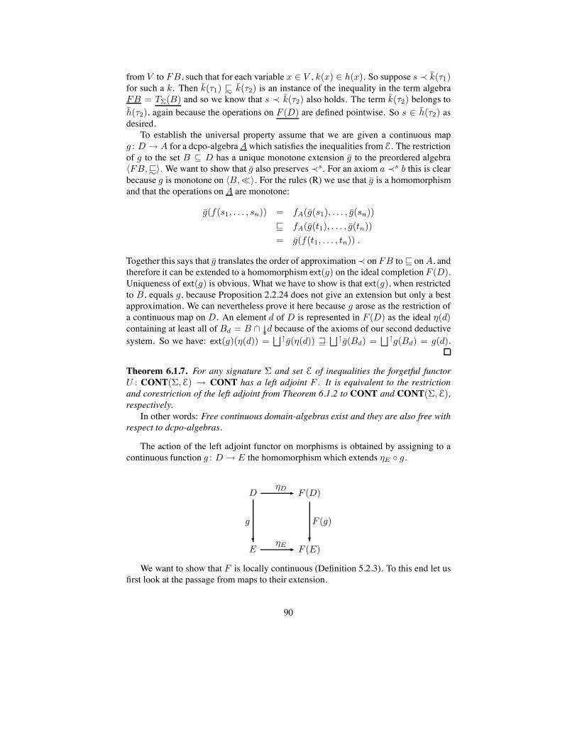
from V to FB, such that for each variable x ! V , k(x) ! h(x). So suppose s @ k(-1)for such a k. Then k(-1) $$ k(-2) is an instance of the inequality in the term algebraFB = T!(B) and so we know that s @ k(-2) also holds. The term k(-2) belongs toh(-2), again because the operations on F (D) are defined pointwise. So s ! h(-2) asdesired.

To establish the universal property assume that we are given a continuous mapg : D " A for a dcpo-algebraAwhich satisfies the inequalities from E. The restrictionof g to the set B 1 D has a unique monotone extension g to the preordered algebra,FB, $$-. We want to show that g also preserves @s. For an axiom a @s b this is clearbecause g is monotone on ,B,:-. For the rules (R) we use that g is a homomorphismand that the operations on A are monotone:

g(f(s1, . . . , sn)) = fA(g(s1), . . . , g(sn))

& fA(g(t1), . . . , g(tn))

= g(f(t1, . . . , tn)) .

Together this says that g translates the order of approximation@ on FB to& onA, andtherefore it can be extended to a homomorphism ext(g) on the ideal completion F (D).Uniqueness of ext(g) is obvious. What we have to show is that ext(g), when restrictedto B, equals g, because Proposition 2.2.24 does not give an extension but only a bestapproximation. We can nevertheless prove it here because g arose as the restriction ofa continuous map on D. An element d of D is represented in F (D) as the ideal .(d)containing at least all of Bd = B * 00d because of the axioms of our second deductivesystem. So we have: ext(g)(.(d)) =

"

#g(.(d)) +"

#g(Bd) ="

#g(Bd) = g(d).

Theorem 6.1.7. For any signature " and set E of inequalities the forgetful functorU : CONT(", E) " CONT has a left adjoint F . It is equivalent to the restrictionand corestriction of the left adjoint from Theorem 6.1.2 to CONT and CONT(", E),respectively.

In other words: Free continuous domain-algebras exist and they are also free withrespect to dcpo-algebras.

The action of the left adjoint functor on morphisms is obtained by assigning to acontinuous function g : D " E the homomorphism which extends .E 5 g.

D.D& F (D)

E

g

' .E& F (E)

F (g)

'

We want to show that F is locally continuous (Definition 5.2.3). To this end let usfirst look at the passage from maps to their extension.

90

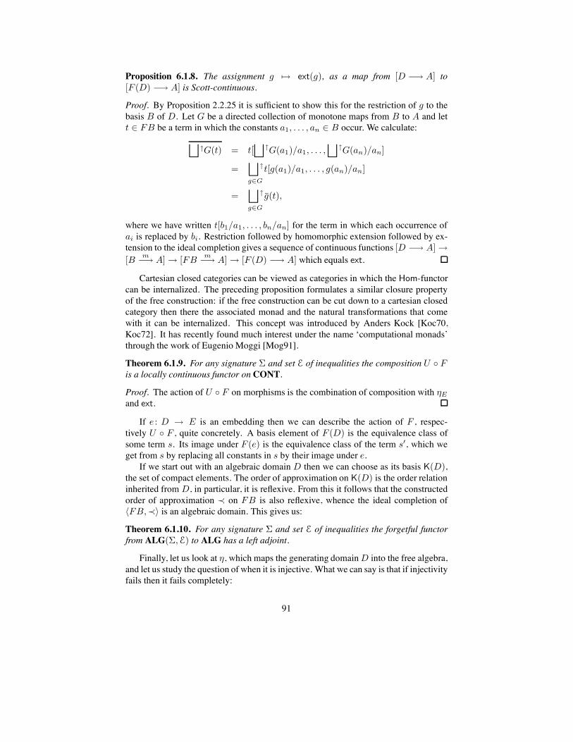
Proposition 6.1.8. The assignment g 9" ext(g), as a map from [D #" A] to[F (D) #" A] is Scott-continuous.

Proof. By Proposition 2.2.25 it is sufficient to show this for the restriction of g to thebasis B of D. Let G be a directed collection of monotone maps from B to A and lett ! FB be a term in which the constants a1, . . . , an ! B occur. We calculate:

$

#G(t) = t[$

#G(a1)/a1, . . . ,$

#G(an)/an]

=$

#

g"G

t[g(a1)/a1, . . . , g(an)/an]

=$

#

g"G

g(t),

where we have written t[b1/a1, . . . , bn/an] for the term in which each occurrence ofai is replaced by bi. Restriction followed by homomorphic extension followed by ex-tension to the ideal completion gives a sequence of continuous functions [D #" A] "[B

m#" A] " [FB

m#" A] " [F (D) #" A] which equals ext.

Cartesian closed categories can be viewed as categories in which the Hom-functorcan be internalized. The preceding proposition formulates a similar closure propertyof the free construction: if the free construction can be cut down to a cartesian closedcategory then there the associated monad and the natural transformations that comewith it can be internalized. This concept was introduced by Anders Kock [Koc70,Koc72]. It has recently found much interest under the name ‘computational monads’through the work of Eugenio Moggi [Mog91].

Theorem 6.1.9. For any signature " and set E of inequalities the composition U 5 Fis a locally continuous functor on CONT.

Proof. The action of U 5 F on morphisms is the combination of composition with .Eand ext.

If e : D " E is an embedding then we can describe the action of F , respec-tively U 5 F , quite concretely. A basis element of F (D) is the equivalence class ofsome term s. Its image under F (e) is the equivalence class of the term s%, which weget from s by replacing all constants in s by their image under e.

If we start out with an algebraic domain D then we can choose as its basis K(D),the set of compact elements. The order of approximation on K(D) is the order relationinherited from D, in particular, it is reflexive. From this it follows that the constructedorder of approximation @ on FB is also reflexive, whence the ideal completion of,FB,@- is an algebraic domain. This gives us:

Theorem 6.1.10. For any signature " and set E of inequalities the forgetful functorfrom ALG(", E) to ALG has a left adjoint.

Finally, let us look at ., which maps the generating domainD into the free algebra,and let us study the question of when it is injective. What we can say is that if injectivityfails then it fails completely:

91

Proposition 6.1.11. For any in-equational theory the canonical map . from a dcpoDinto the free algebra F (D) overD is order-reflecting if and only if there exists a dcpo-algebra A for this theory for which the carrier dcpoA is non-trivially ordered.

Proof. Assume that there exists a dcpo-algebraA which contains two elements a $ b.LetD be any dcpo and x 8& y two distinct elements. We can define a continuous map gfromD to A, separating x from y by setting

g(d) =

&

a, if d & y;b, otherwise.

Since g equals ext(g) 5 ., where ext(g) is the unique homomorphism from F (D) to A,it cannot be that .(x) & .(y) holds.

The converse is trivial, because . must be monotone.

6.1.3 Least elements and strict algebras

We have come across strict functions several times already. It therefore seems worth-while to study the problem of free algebras also in this context. But what should a strictalgebra be? There are several possibilities as to what to require of the operations onsuch an algebra:

1. An operation which is applied to arguments, one of which is bottom, returnsbottom.

2. An operation applied to the constantly bottom vector returns bottom.

3. An operation of arity greater than 0 applied to the constantly bottom vector re-turns bottom.

Luckily, we can leave this open as we shall see shortly. All we need is:

Definition 6.1.12. A strict dcpo-algebra is a dcpo-algebra for which the carrier setcontains a least element. A strict homomorphism between strict algebras is a Scott-continuous homomorphism which preserves the least element.

For pointed dcpo’s the existence of free strict dcpo-algebras can be established asbefore through the Adjoint Functor Theorem. For pointed domains the construction ofthe previous subsection can be adapted by adding a further axiom to the first deductionscheme:

(A3) . $$ t for all t ! FB.

Thus we have:

Theorem 6.1.13. Free strict dcpo- and domain-algebras exist, that is, the forgetfulfunctors

DCPO$!(", E) #" DCPO$!,

CONT$!(", E) #" CONT$!,

and ALG$!(", E) #" ALG$!

have left adjoints.

92

Let us return to the problem of strict operations. The solution is that we can adda nullary operation 0 to the signature and the inequality 0 & x to E without changingthe free algebras. Because of axiom (A3) we have . $$ 0 and because of the newinequality we have 0 $$ .. Therefore the new operation must be interpreted by thebottom element. The advantage of having bottom explicitly in the signature is thatwe can now formulate equations about strictness of operations. For example, the firstpossibility mentioned at the beginning can be enforced by adding to E the inequality

f(x1, . . . , xi&1, 0, xi+1, . . . , x#(f)) & 0

for all operation symbols f of positive arity and all 1 ) i ) #(f). The correspondingfree algebras then exist by the general theorem.

More problematic is the situation with DCPO$ (respectively CONT$ andALG$). The existence of a least element in the generating dcpo does not imply theexistence of a least element in the free algebra (Exercise 6.2.23(2)). Without it, wecannot make use of local continuity in domain equations. Furthermore, even if the freealgebra has a least element, it need not be the case that . is strict (Exercise 6.2.23(3)).The same phenomena appears if we restrict attention to any of the cartesian closed cat-egories exhibited in Chapter 4. The reason is that we require a special structure of theobjects of our category but allow morphisms which do not preserve this structure. It istherefore always an interesting fact if the general construction for a particular algebraictheory can be restricted and corestricted to one of these sub-categories. In the casethat the general construction does not yield the right objects it may be that a differentconstruction is needed. This has been tried for the Plotkin powerdomain in severalattempts by Karel Hrbacek but a satisfactory solution was obtained only at the cost ofchanging the morphisms between continuous algebras, see [Hrb87, Hrb89, Hrb88].

On a more positive note, we can say:

Proposition 6.1.14. If the free functor maps finite pointed posets to finite pointed posetsthen it restricts and corestricts to bifinite domains.

6.2 Powerdomains6.2.1 The convex or Plotkin powerdomain

Definition 6.2.1. The convex or Plotkin powertheory is defined by a signature with onebinary operation 6 and the equations

1. x 6 y = y 6 x (Commutativity)

2. (x 6 y) 6 z = x 6 (y 6 z) (Associativity)

3. x 6 x = x (Idempotence)

The operation 6 is called formal union.A dcpo-algebra with respect to this theory is called a dcpo-semilattice. The free

dcpo-semilattice over a dcpo D is called the Plotkin powerdomain of D and it is de-noted by PP(D).

93

Every semilattice can be equipped with an order by setting

x ) y if x 6 y = y.

Formal union then becomes the join in the resulting ordered set. On a dcpo-semilatticethis order has little to do with the domain ordering and it is not in the focus of ourinterest.

The free semilattice over a set X is given by the set of all non-empty finite subsetsof X , where formal union is interpreted as actual union of sets. This gives us thefirst half of an alternative description of the Plotkin powerdomain over a continuousdomain D with basis B. Its basis FB, which we constructed as the term algebraover B, is partitioned into equivalence classes by F, the equivalence relation derivedfrom $$, that is, from the defining equations. These equivalence classes are in one-to-one correspondence with finite subsets of B. Indeed, given a term from FB, we canre-arrange it because of associativity and commutativity, and because of idempotencewe can make sure that each constant occurs just once.

Remember that we have set up the order of approximation@ onFB as the transitiveclosure of $$ 5 @s 5 $$. This way we have ensured that an ideal in FB contains onlyfull equivalence classes with respect to F. We may therefore replace FB by Pf (B),the set of finite subsets of B, where we associate with a term t ! FB the set [t] ofconstants appearing in t.

Let us now also transfer the order of approximation to the new basis.

Definition 6.2.2. Two subsets M and N of a set equipped with a relation R are inthe Egli-Milner relation, written as M REM N , if the following two conditions aresatisfied:

>a ! M ?b ! N. a R b

>b ! N ?a ! M. a R b.

Here we are talking about finite subsets of ,B,:-, so we write:EM for the Egli-Milner relation between finite subsets of B. Let us establish the connection between:EM on Pf (B) and @ on FB. Firstly, if s @s t then by definition each constantin t is matched by a constant in s which approximates it and vice versa. These are justthe conditions for [s] :EM [t]. Since:EM is transitive, we find that s @ t implies[s] :EM [t] in general. Conversely, if two finite subsets M = {a1, . . . , am} andN = {b1, . . . , bn} ofB are related by:EM then we can build terms s and t, such that[s] = M , [t] = N , and s @s t hold. This is done as follows. For each ai ! M let bj(i)

be an element of N such that ai : bj(i) and for each bj ! N let ai(j) be an elementofM such that ai(j) : bj . Then we can set

s = (a1 6 . . . 6 am) 6 (ai(1) 6 . . . 6 ai(n))

and t = (bj(1) 6 . . . 6 bj(m)) 6 (b1 6 . . . 6 bn).

We have proved:

Theorem 6.2.3. The Plotkin powerdomain of a continuous domain D with basis,B,:- is given by the ideal completion of ,Pf (B),:EM -.

94

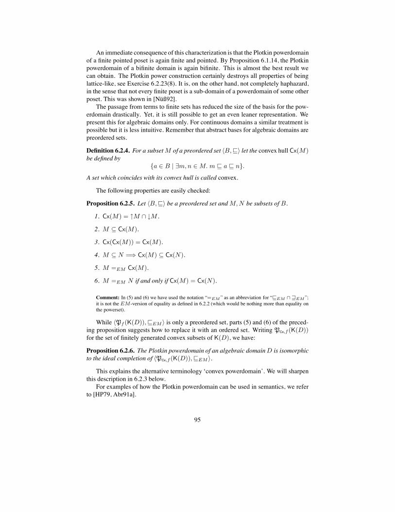
An immediate consequence of this characterization is that the Plotkin powerdomainof a finite pointed poset is again finite and pointed. By Proposition 6.1.14, the Plotkinpowerdomain of a bifinite domain is again bifinite. This is almost the best result wecan obtain. The Plotkin power construction certainly destroys all properties of beinglattice-like, see Exercise 6.2.23(8). It is, on the other hand, not completely haphazard,in the sense that not every finite poset is a sub-domain of a powerdomain of some otherposet. This was shown in [Nuß92].

The passage from terms to finite sets has reduced the size of the basis for the pow-erdomain drastically. Yet, it is still possible to get an even leaner representation. Wepresent this for algebraic domains only. For continuous domains a similar treatment ispossible but it is less intuitive. Remember that abstract bases for algebraic domains arepreordered sets.

Definition 6.2.4. For a subsetM of a preordered set ,B,&- let the convex hull Cx(M)be defined by

{a ! B | ?m, n ! M. m & a & n}.

A set which coincides with its convex hull is called convex.

The following properties are easily checked:

Proposition 6.2.5. Let ,B,&- be a preordered set andM, N be subsets of B.

1. Cx(M) = /M * 0M .

2. M 1 Cx(M).

3. Cx(Cx(M)) = Cx(M).

4. M 1 N =( Cx(M) 1 Cx(N).

5. M =EM Cx(M).

6. M =EM N if and only if Cx(M) = Cx(N).

Comment: In (5) and (6) we have used the notation “=EM ” as an abbreviation for “(EM ) *EM ”;it is not the EM -version of equality as defined in 6.2.2 (which would be nothing more than equality onthe powerset).

While ,Pf (K(D)),&EM - is only a preordered set, parts (5) and (6) of the preced-ing proposition suggests how to replace it with an ordered set. Writing PCx,f (K(D))for the set of finitely generated convex subsets of K(D), we have:

Proposition 6.2.6. The Plotkin powerdomain of an algebraic domainD is isomorphicto the ideal completion of ,PCx,f (K(D)),&EM -.

This explains the alternative terminology ‘convex powerdomain’. We will sharpenthis description in 6.2.3 below.

For examples of how the Plotkin powerdomain can be used in semantics, we referto [HP79, Abr91a].

95

6.2.2 One-sided powerdomains

Definition 6.2.7. If the Plotkin powertheory is augmented by the inequality

x & x 6 y

then we obtain the Hoare or lower powertheory. Algebras for this theory are calledinflationary semilattices. The free inflationary semilattice over a dcpo D is called thelower or Hoare powerdomain of D, and it is denoted by PH(D).

Similarly, the terminology concerning the inequality

x + x 6 y

is upper or Smyth powerdomain, deflationary semilattice, and PS(D).

It is a consequence of the new inequality that the semilattice ordering and the do-main ordering coincide in the case of the Hoare powertheory. For the Smyth powerthe-ory the semilattice ordering is the reverse of the domain ordering. This forces thesepowerdomains to have additional structure.

Proposition 6.2.8. 1. The Hoare powerdomain of any dcpo is a lattice which hasall non-empty suprema and bounded infima. The sup operation is given by formalunion.

2. The Smyth powerdomain of any dcpo has binary infima. They are given by formalunion.

Unfortunately, the existence of binary infima does not force a domain into one ofthe cartesian closed categories of Chapter 4. We take up this question again in the nextsubsection.

Let us also study the bases of these powerdomains as derived from a given basis,B,:- of a continuous domain D. The development proceeds along the same linesas for the Plotkin powertheory. The equivalence relation induced by the equations andthe new inequality has not changed, so we may again replace FB by the set Pf (B) offinite subsets of B. The difference is wholly in the associated preorder on Pf (B).

Proposition 6.2.9. For M andN finite subsets of a basis ,B,:- we have

M $$ N if and only if M 1 0N

in the case of the Hoare powertheory and

M $$ N if and only if N 1 /M

for the Smyth powertheory.

The restricted order of approximation @s is as before given by the Egli-Milnerrelation:EM . As prescribed by the general theory we must combine it with inclusion(for the lower theory) and with reversed inclusion (for the upper theory), respectively.Without difficulties one obtains the following connection

s @H t if and only if >a ! [s] ?b ! [t]. a : b

96

ands @S t if and only if >b ! [t] ?a ! [s]. a : b.

So each of the one-sided theories is characterized by one half of the Egli-Milner order-ing. Writing:H and:S for these we can formulate:

Theorem 6.2.10. Let D be a continuous domain with basis ,B,:-.

1. The Hoare powerdomain of D is isomorphic to the ideal completion of,Pf (B),:H-.

2. The Smyth powerdomain of D is isomorphic to the ideal completion of,Pf (B),:S-.

For algebraic domains we can replace the preorders on Pf(B) by an ordered set inboth cases.

Proposition 6.2.11. For subsets M andN of a preordered set ,B,)- we have

1. M =H 0M ,

2. M )H N if and only if 0M 1 0N ,

and

3. M =S /M ,

4. M )S N if and only if /M < /N .

Writing PL,f(B) for the set of finitely generated lower subsets of B andPU,f(B)for the set of finitely generated upper subsets of B, we have:

Proposition 6.2.12. Let D be an algebraic domain.

1. The Hoare powerdomain PH(D) of D is isomorphic to the ideal completion of,PL,f (K(D)),1-.

2. The Smyth powerdomain PS(D) of D is isomorphic to the ideal completion of,PU,f (K(D)),<-.

From this description we can infer through Proposition 6.1.14 that the Smyth pow-erdomain of a bifinite domain is again bifinite. Since a deflationary semilattice hasbinary infima anyway, we conclude that the Smyth powerdomain of a bifinite domainis actually a bc-domain. For a more general statement see Corollary 6.2.15.

6.2.3 Topological representation theorems

The objective of this subsection is to describe the powerdomains we have seen so fardirectly as spaces of certain subsets of the given domain, without recourse to basesand the ideal completion. It will turn out that the characterizations of Proposition 6.2.6and Proposition 6.2.12 can be extended nicely once we allow ourselves topologicalmethods.

97

Theorem 6.2.13. The Hoare powerdomain of a continuous domainD is isomorphic tothe lattice of all non-empty Scott-closed subsets of D. Formal union is interpreted byactual union.

Proof. Let ,B,:- be a basis for D. We establish an isomorphism with the repre-sentation of Theorem 6.2.10. Given an ideal I of finite sets in PH(D) we map it to%H(I) = Cl(

!

I), the Scott-closure of the union of all these sets. Conversely, for anon-empty Scott-closed set A we let ,H(A) = Pf (00A * B), the set of finite sets ofbasis elements approximating some element in A. We first check that ,H(A) is in-deed an ideal with respect to:H . It is surely non-empty as A was assumed to containelements. Given two finite subsets M and N of 00A * B then we can apply the inter-polation axiom to get finite subsets M % and N % with M :EM M % and N :EM N %.An upper bound forM andN with respect to:H is then given byM % 6N %. It is alsoclear that the Scott closure of 00A * B gives A back again because every element ofDis the directed supremum of basis elements. Hence %H 5,H = id. Starting out with anideal I , we must show that we get it back from %H(I). So letM ! I . By the roundnessof I (see the discussion before Definition 2.2.21) there is another finite setM % ! I withM :H M %. So for each a ! M there is b ! M % with a : b. Since all elements of Iare contained in %H(I), we have that a belongs to 00%(I) * B. Conversely, if a is anelement of 00%(I) * B then //a * %(I) is not empty and therefore must meet

!

I asD \ //a is closed. The set {a} is then below some element of I under the:H -ordering.Monotonicity of the isomorphisms is trivial and the representation is proved.

Formal union applied to two ideals returns the ideal of unions of the constitutingsets. Under the isomorphism this operation is transformed into union of closed subsets.

This theorem holds not just for continuous domains but also for all dcpo’s and evenall T0-spaces. See [Sch93] for this. We can also get the full complete lattice of allclosed sets if we add to the Hoare powertheory a nullary operation e and the equations

e 6 x = x 6 e = x.

Alternatively, we can take the strict free algebra with respect to the Hoare powertheory.If the domain has a least element then these adjustments are not necessary, a leastelement for the Hoare powerdomain is {.}. Homomorphisms, however, will onlypreserve non-empty suprema.

The characterization of the Smyth powerdomain builds on the material laid out inSection 4.2.3. In particular, recall that a Scott-compact saturated set in a continuousdomain has a Scott-open filter of open neighborhoods and that each Scott-open filterin )D arises in this way.

Theorem 6.2.14. The Smyth powerdomain of a continuous domain D is isomorphicto the set +D \ {B} of non-empty Scott-compact saturated subsets ordered by reversedinclusion. Formal union is interpreted as union.

Proof. Let ,B,:- be a basis forD. We show that +D \ {B} is isomorphic to PS(D) =Idl(Pf (B),:S). Given an ideal I we let %S(I) be

#

M"I /M . This constitutes a

98

monotone map from PS(D) to +D \ {B} by Proposition 4.2.14. In the other direction,we assign to a compact saturated set A the set ,S(A) of all finite setsM 1 B such thatA 1 //M . Why is this an ideal? For every open neighborhood O of A we find a finitesetM of basis elements contained in O such that A 1 //M because A is compact andO =

!

b"O'B//b (Proposition 2.3.6). Then given two finite sets M and N in ,S(A)

an upper bound for them is any such finite set P with A 1 //P 1 //M * //N . Clearly,,S is monotone as +D \ {B} is equipped with reversed inclusion.

Let us show that ,S 5%S is the identity on PS(D). ForM ! I letM % ! I be aboveM in the:S-ordering. Then %S(I) 1 /M % 1 //M and soM belongs to ,S 5 %S(I).Conversely, every neighborhood of %S(I) contains some /M with M ! I already aswe saw in Proposition 4.2.14. So if %S(I) is contained in //N for some finite setN 1 Bthen there are M and M % in I with M 1 //N andM :S M %. Hence N :S M % andN belongs to I .

The composition %S 5,S is clearly the identity as we just saw that every neighbor-hood of a compact set contains a finitely generated one and as every saturated set is theintersection of its neighborhoods.

The claim about formal union follows because on powersets union and intersectioncompletely distribute: %S(I 6 J) =

#

M"I,N"J /(M 6 N) =#

M"I,N"J(/M 6

/N) =#

M"I /M 6#

N"J /N = %S(I) 6 %S(J).

For this theorem continuity is indispensable. A characterization of the free defla-tionary semilattice over an arbitrary dcpo is not known. The interested reader mayconsult [Hec90, Hec93a] and [Sch93] for a discussion of this open problem.

Corollary 6.2.15. The Smyth powerdomain of a coherent domain with bottom is abc-domain.

Proof. That two compact saturated sets A and B are bounded by another one, C, sim-ply means C 1 A * B. In this case A * B is not empty. It is compact saturated by thevery definition of coherence.

Let us now turn to the Plotkin powerdomain. An ideal I of finite sets orderedby :EM will generate ideals with respect to both coarser orders :H and :S . Wecan therefore associate with I a Scott-closed set %H(I) = Cl(

!

I) and a compactsaturated set %S(I) =

#

M"I /M . However, not every such pair arises in this way; thePlotkin powerdomain is not simply the product of the two one-sided powerdomains.We will be able to characterize them in two special cases: for countably based domainsand for coherent domains. The general situation is quite hopeless, as is illustratedby Exercise 6.2.23(11). In both special cases we do want to show that I is faithfullyrepresented by the intersection %(I) = %H(I) * %S(I). In the first case we will needthe following weakening of the Egli-Milner ordering:

Definition 6.2.16. For a dcpo D we let Lens(D) be the set of all non-empty subsetsof D which arise as the intersection of a Scott-closed and a compact saturated subset.The elements of Lens(D) we call lenses. On Lens(D) we define the topological Egli-Milner ordering,&TEM , by

K &TEM L if L 1 /K andK 1 Cl(L).

99

Proposition 6.2.17. Let D be a dcpo.

1. Every lens is convex and Scott-compact.

2. A canonical representation for a lens L is given by /L * Cl(L).

3. The topological Egli-Milner ordering is anti-symmetric on Lens(D).

Proof. Convexity is clear as every lens is the intersection of a lower and an upper set.An open covering of a lens L = C * U , where C is closed and U compact saturated,may be extended to a covering of U by adding the complement of C to the cover.This proves compactness. Since all Scott-open sets are upwards closed, compactnessof a set A implies the compactness of /A. Using convexity, we get L = /L * 0L 1/L * Cl(L) and using boolean algebra we calculate /L = /(C * U) 1 /U = U andCl(L) = Cl(C *U) 1 Cl(C) = C, so /L*Cl(L) 1 U *C = L. Then ifK =TEM Lwe have /K = /L and Cl(K) = Cl(L). Equality ofK and L follows.

Before we can prove the representation theorem we need yet another description ofthe lens %(I).

Lemma 6.2.18. Let D be a continuous domain with basis B and let I be an ideal in,Pf (B),:EM -. Then %(I) = {

"

#A | A 1!

I directed and A * M 8= B for allM ! I}.

Proof. The elements of the set on the right clearly belong to the Scott-closure of!

I .They are also contained in %S(I) because

"

#A is above some element in A * M foreachM ! I .

Conversely, let x ! %(I) and let a ! A = 00x * B. The set //a is Scott-open andmust therefore meet some M ! I . From the roundness of I we get M % ! I withM :EM M %. The set M 6 {a} also approximates M % and so it is contained in I .Hence a !

!

I . Furthermore, given any M ! I , let again M % ! I be such thatM :EM M %. Then x is above some element of M % as %(I) 1 /M % and thereforem : x holds for somem ! M .

Theorem 6.2.19. LetD be an "-continuous domain. The Plotkin powerdomainPP(D)is isomorphic to ,Lens(D),&TEM -. Formal union is interpreted as union followed bytopological convex closure.

Proof. Let ,B,:- be a countable basis of D. We have already defined the map% : PP(D) " Lens(D). In the other direction we take the function, which assigns to alensK the set ,H(Cl(K))* ,S(/K). Before we can prove that these maps constitutea pair of isomorphisms, we need the following information about reconstructing %H(I)and %S(I) from %(I).

1. %S(I) = /%(I): Since %S(I) is an upper set which contains %(I), only oneinclusion can be in doubt. Let x ! %S(I) and I % = {M * 0x | M ! I}. Firstly,each set in I % is non-empty and, secondly, we have M * 0x :S N * 0x wheneverM :EM N . Calculating %S(I %) in the continuous domain %H(I) gives us a non-empty set which is below x and contained in the lens %(I).

100

2. %H(I) = Cl(%(I)): Again, only one inclusion needs an argument. We show thatevery element of 00%H(I)*B belongs to 0%(I). Given a basis element a approximatingsome element of %H(I) then we already know that it belongs to

!

I . Let M ! I besome set which contains a. Using countability of the basis we may assume that Mextends to a cofinal chain in I (Proposition 2.2.13): M = M0 :EM M1 :EM

M2 :EM . . . . Konig’s Lemma then tells us that we can find a chain of elementsa = a0 : a1 : a2 : . . . where an ! An. The supremum x =

"

#n"N

an belongs to%(I) and is above a.

3. % is monotone: Let I 1 I % be two ideals in ,Pf (B),:EM -. The larger idealresults in a bigger lower set %H(I %) and a smaller upper set %S(I %). Using 1 and 2 wecan calculate for the corresponding lenses:

%(I) 1 %H(I) 1 %H(I %) = Cl(%(I %)),

%(I %) 1 %S(I %) 1 %S(I) = /%(I).

So %(I) &TEM %(I %) as desired.4. The monotonicity of , follows by construction and one half of the topological

Egli-Milner ordering: K 1 /M implies L 1 /M if we assumeK &TEM L.5. % 5 , = id: Given a lens L = C * U we clearly have %S(,(L)) < L. Using

the continuity of D and the compactness of L we infer that %S(,(L)) must equal /L.Every basis element approximating some element of L occurs in some set of ,(L), so%H(,(L)) = Cl(L) is clear. Proposition 6.2.17 above then implies that % 5,(L) givesback L.

6. , 5 % = id: Given an ideal I we know that each M ! I covers the lens %(I)in the sense of //M < %(I). So M is contained in ,S(%(I)). By (2), we also havethat M is contained in ,H(Cl(%(I))). Conversely, if //M < %(I) for a finite set Mof basis elements contained in 00%(I), then for some N ! I we have //M < N by theHofmann-Mislove Theorem 4.2.14. For thisN we haveM :S N . On the other hand,each element a ofM approximates some x ! %(I) and hence belongs to someNa ! I .An upper bound for N and all Na in I , therefore, is above M in:EM which showsthatM must belong to I .

7. In the representation theorems for the one-sided powerdomains we have shownthat formal union translates to actual union. We combine this for the convex setting:%(I 6 J) = %H(I 6 J) * %S(I 6 J) = (%H(I) 6 %H(J)) * (%S(I) 6 %S(J)) =(Cl(%(I)) 6 Cl(%(J))) * (/%(I) 6 /%(J)) = Cl(%(I) 6 %(J)) * /(%(I) 6 %(J)).

Note that we used countability of the basis only for showing that %H(I) can berecovered from %(I). In general, this is wrong. Exercise 6.2.23(11) discusses an ex-ample.

The substitution of topological closure for downward closure was also necessary,as the example in Figure 13 shows. There, the set A = /a is a lens but its downwardclosure is not Scott-closed, c is missing. The set A 6 {c} is also a lens. It is below Ain the topological Egli-Milner order but not in the plain Egli-Milner order. The convexclosure of the union of the two lenses {.} and A is not a lens, c must be added.

A better representation theorem is obtained if we pass to coherent domains (Sec-tion 4.2.3). (Note that the example in Figure 13 is not coherent, because the set

101

' .

' a

'a1'a2'a3

'c1

'c2

'c3

'c """"""

"""

""

""

""!

!!

$$

$$

$$""

""!! !

!!

!!!"

""!!

Figure 13: An algebraic domain in which topological Egli-Milner ordering and ordi-nary Egli-Milner ordering do not coincide.

{c1, a} has infinitely many minimal upper bounds, violating the condition in Proposi-tion 4.2.17.) We first observe that lenses are always Lawson closed sets. If the domainis coherent then this implies that they are also Lawson-compact. Compactness willallow us to use downward closure instead of topological closure.

Lemma 6.2.20. Let L be a Lawson-compact subset of a continuous domain D. Then0L is Scott-closed.

Proof. Let x be an element of D which does not belong to 0L. For each y ! L thereexists by : x such that by 8& y. The set D \ /by is Lawson-open and contains y.By compactness, finitely many such sets cover L. Let b be an upper bound for theassociated basis elements approximating x. Then //b is an open neighborhood of xwhich does not intersect L. Hence 0L is closed.

Corollary 6.2.21. The lenses of a coherent domain are precisely the convex Lawson-compact subsets. For these, topological Egli-Milner ordering and Egli-Milner orderingcoincide.

Theorem 6.2.22. Let D be a coherent domain. The Plotkin powerdomain of D isisomorphic to ,Lens(D),&EM -. Formal union is interpreted as union followed byconvex closure.

Proof. The differences to the proof of Theorem 6.2.19, which are not taken care ofby the preceding corollary, concern part 2. We must show that Cl(%(I)) = 0%(I)contains all of 00%H(I) * B. In the presence of coherence this can be done throughthe Hofmann-Mislove Theorem 4.2.14. The lower set %H(I) is a continuous domainin itself. For an element a of 00%H(I) * B we look at the filtered collection of uppersets J = {/a * /M | M ! I}. Each of these is non-empty, because a belongs to someM ! I , and compact saturated because of coherence. Hence

#

J is non-empty. It isalso contained in %(I) and above a.

102

6.2.4 Hyperspaces and probabilistic powerdomains

In our presentation of powerdomains we have emphasized the feature that they are freealgebras with respect to certain (in-)equational theories. From the general existencetheorem for such algebras we derived concrete representations as sets of subsets. Thisis the approach which in the realm of domain theory was suggested first by MatthewHennessy and Gordon Plotkin in [HP79] but it has a rather long tradition in algebraicsemantics (see e.g. [NR85]). However, it is not the only viewpoint one can take. Onemay also study certain sets of subsets of domains in their own right. In topology,this study of ‘hyperspaces’, as they are called, is a long-standing tradition, startingwith Felix Hausdorff [Hau14] and Leopold Vietoris [Vie21, Vie22]. It is also how thesubject started in semantics and, indeed, continues to be developed. A hyperspace canbe interesting even if an equational characterization cannot be found or can be foundonly in restricted settings. Recent examples of this are the set-domains introduced byPeter Buneman [BDW88, Gun92a, Hec90, Puh93, Hec91, Hec93b] in connection witha general theory of relational databases. While these are quite natural from a domain-theoretic point of view, their equational characterizations (which do exist for some ofthem) are rather bizarre and do not give us much insight. The hyperspace approach isdeveloped in logical form in Section 7.3.

We should also mention the various attempts to define a probabilistic version ofthe powerdomain construction, see [SD80, Mai85, Gra88, JP89, Jon90]. (As an aside,these cannot be restricted to algebraic domains; the wider concept of continuous do-main is forced upon us through the necessary use of the unit interval [0, 1].) They dohave an equational description in some sense but this goes beyond the techniques ofthis chapter.

One can then ask abstractly what constitutes a powerdomain construction and builda theory upon such a definition. This approach was taken in [Hec90, Hec91]. Themost notable feature of this work is that under this perspective, too, many of the knownpowerdomains turn out to be canonical in a precise sense. How this (very natural)formulation of canonicity is connected with concerns in semantics, however, is as yetunclear.

Exercises 6.2.23. 1. For the proof of Theorem 6.1.6 we can equip FB also withthe transitive closure of@s 5 $$. Show:

(a) This relation@% satisfies the interpolation axiom.(b) In general,@% is different from @.(c) The ideal completions of ,FB,@- and ,FB,@%- are isomorphic. (Use

Exercise 2.3.9(27).)(d) What is the advantage of @ over @%?

2. Describe the free domain algebra for an arbitrary domain D and an arbitrarysignature " in the case that E is empty.

3. Set up an algebraic theory such that all its dcpo-algebras have least elementsbut the embeddings . are not strict.

103

'' '

'

- a

- -- -

..

..+

+++ .

...

!!!

++

++>>>>>>>%

%%..

..

%%%"

"" ######>>>>>>>

..

.. ++

++

./

01

./

01

./

01

./

01

Figure 14: Part of an algebraic domain where Theorem 6.2.19 fails.

4. Let ,", E- be the usual equational theory of groups (or boolean algebras). Showthat any dcpo-algebra with respect to this theory is trivially ordered. Concludethat the free construction collapses each connected component of the generatingdcpo into a single point.

5. Given signatures " and "% and sets of inequalities E and E% we call the pair,", E- a reduct of ,"%, E%- if " 1 "% and E 1 E%. In this case there is an obviousforgetful functor from C("%, E%) to C(", E), where C is any of the categoriesconsidered in this chapter. Show that the general techniques of Theorem 6.1.2and 6.1.7 suffice to prove that this functor has a left adjoint.

6. Likewise, show that partial domain algebras can be completed freely.

7. Let A be a free domain-algebra over an algebraic domain. Is it true that everyoperation, if applied to compact elements of A, returns a compact element?

8. Let D = {. & a, b & =} be the four-element lattice (Figure 1) and let E =D%D. The sets {,., a-, ,., b-} and {,a,.-, ,b,.-} are elements of the Plotkinpowerdomain of E. Show that they have two minimal upper bounds. Since{,=,=-} is a top element, PP(E) is not an L-domain.

9. Is the Plotkin powerdomain closed on F-B, the category whose objects are bilim-its of finite (but not necessarily pointed) posets?

10. Define a natural isomorphism between PH(D)$#3E and [D #" E] whereD isany continuous domain, E is a complete lattice, and ·#3· stands for the set offunctions which preserve all suprema (ordered pointwise).

11. We want to construct an algebraic domain D to which Theorem 6.2.19 cannotbe extended. The compact elements ofD are arranged in finite sets already suchthat they form a directed collection in the Egli-Milner ordering, generating theideal I . We take one finite set for each element of Pf(R), the finite powersetof the reals (or any other uncountable set), and we will have M# :EM M$ if# 1 $ 1 R. So we can arrange the M# in layers according to the cardinalityof #. Each M# contains one ‘white’ and |#|! many ‘black’ elements. If # " $then the white element of M# is below every element of M$ . For the orderbetween black elements look at adjacent layers. There are |$| many subsets of $

104

with cardinality |$| # 1. The |$|! many black elements of M$ we partition into|$| many classes of cardinality (|$| # 1)!. So we can let the black elements of alower neighbor of M$ be just below the equally many black elements of one ofthese classes. (The idea being that no two black elements have an upper bound.)Figure 14 shows a tiny fraction of the resulting ordered set K(D). Establish thefollowing facts about this domain:

(a) Above a black element there are only black, below a white element thereare only white elements.

(b) i. An ideal inK(D) can contain at most one black element from each set.ii. An ideal can contain at most one black element in each layer.iii. An ideal can contain at most countably many black elements.

(c) i. An ideal meeting all sets must contain all white elements.ii. If an ideal contains a black element, then it contains the least black

element a.iii. If an ideal meeting all sets contains a then it must contain upper

bounds for a and the uncountably many white elements of the firstlayer. These upper bounds must form an uncountable set and consistsolely of black elements.

(d) From the contradiction between b-iii and c-iii conclude that only one idealin KD meets all sets, the ideal W of white elements. Therefore, %(I) con-tains precisely one element, say b. Show that 0b equalsW 6 {b} and that itis Scott-closed. Hence it is far from containing all elements of

!

I = KD.(e) Go a step farther and prove that the lenses of D are not even directed-

complete by showing that the ideal I we started out with does not have anupper bound.

12. (R. Heckmann) Remove idempotence from the Hoare powertheory and study freedomain algebras with respect to this theory. These are no longer finite if thegenerating domain is finite. Show that the free algebra over the four-elementlattice (Figure 1) is neither bifinite nor an L-domain.

105

7 Domains and logicThere are at least three ways in which the idea of a function can be formalized. The firstis via algorithms, which is the Computer Science viewpoint. The second is via valuetables or, in more learned words, via graphs. This is the – rather recent – invention ofMathematics. The third, finally, is via propositions: We can either take propositionsabout the function itself or view a function as something which maps arguments whichsatisfy % to values which satisfy ,. The encoding in the latter case is by the set of allsuch pairs (%,,). The beauty of the subject, then, lies in the interplay between thesenotions.

The passage from algorithms (programs) to the extensional description via graphsis called denotational semantics. It requires sophisticated structures, precisely domainsin the sense of this text, because of, for example, recursive definitions in programs. Thepassage from algorithms to propositions about functions is called program logics. Ifwe take the computer scientist’s point of view as primary then denotational semanticsand program logics are two different ways of describing the behaviour of programs.It is the purpose of this chapter to lay out the connection between these two forms ofsemantics. As propositionswe allow all those formulaewhose extensions in the domainunder consideration are (compact) Scott-open sets. This choice is well justified becauseit can be argued that such propositions correspond to properties which can be detectedin a finite amount of time [Abr87]. The reader will find lucid explications of this pointin [Smy92] and [Vic89].

Mathematically, then, we have to study the relation between domains and theircomplete lattices of Scott-open sets. Stated for general topological spaces, this is thefamous Stone duality. We treat it in Section 7.1. The restriction to domains introducesseveral extra features which we discuss in a one by one fashion in Section 7.2. Theactual domain logic, as a syntactical theory, is laid out in Section 7.3.

The whole open-set lattice, however, is too big to be syntactically represented.We must, on this higher level, once more employ ideas of approximation and bases.There is a wide range of possibilities here, which can be grouped under the headingof information systems. We concentrate on one of these, namely, the logic of compactopen subsets. This is well motivated by the general framework of Stone duality andalso gives the richest logic.

7.1 Stone duality7.1.1 Approximation and distributivity

We start out with a few observations concerning distributivity. So far, this didn’t play arole due to the poor order theoretic properties of domains. Now, in the context of openset lattices, it becomes a central theme, because, as we shall see, it is closely relatedwith the concept of approximation. The earliest account of this connection is probably[Ran53].

A word on notation: We shall try to keep a clear distinction between spaces, whichin the end will be our domains, and their open-set lattices. We shall emphasize thisby using ) for the less-than-or-equal-to relation whenever we speak of lattices, even

106

though these do form a special class of domains, too, as you may remember fromSection 4.1.

Recall that a lattice L is said to be distributive if for all x, y, z ! L the equality

x ' (y G z) = (x ' y) G (x ' z)

holds. The dual of this axiom is then satisfied as well. For the infinitary version ofdistributivity, we introduce the following notation for choice functions: If (Ai)i"I is afamily of sets then we write f : I

4#"

!

Ai if f(i) takes its value inAi for every i ! I .Complete distributivity can then be expressed by the equation

-

i"I

.

Ai =.

f : I$

&56Ai

-

i"I

f(i).

It, too, implies its order dual, see Exercise 7.3.19(1). There is a lot of room for varia-tions of this and we shall meet a few of them in this section. Here comes the first:

Theorem 7.1.1. A complete lattice L is continuous if and only if-

i"I

.

#Ai =.

#

f : I$

&56Ai

-

i"I

f(i)

holds for all families (Ai)i"I of directed subsets of L.

Proof. The reader should check for himself that the supremum on the right hand sideis indeed over a directed set. Let now x be an element approximating the left handside of the equation. Then for each i ! I we have x :

/

#Ai and so there is ai !Ai with x ) ai. Let f be the choice function which selects these ai. Then x )0

i"I f(i) and x is below the right hand side as well. Assuming L to be continuous,this proves

0

i"I

/

#Ai )/

#f : I

$&56Ai

0

i"I f(i). The reverse inequality holds inevery complete lattice.

For the converse fix an element x ! L and let (Ai)i"I be the family of all directedsets A for which x )

/

#A. From the equality, which we now assume to hold, we getthat x =

/

#f : I

$&56Ai

0

f(i). We claim that for each choice function f : I4#"

!

Ai,the corresponding element y =

0

i"I f(i) is approximating x. Indeed, ifA is a directedset with x )

/

#A then A = Ai0 for some i ! I and so y ) f(i0) ! A.

Let us now look at completely distributive lattices which, by the preceding the-orem, are guaranteed to be continuous. We can go further and express this strongerdistributivity by an approximation axiom, too.

Definition 7.1.2. For a complete lattice L define a relation% on L by

x % y if >A 1 L. (y ).

A =( ?a ! A. x ) a).

Call L prime-continuous if for every x ! L, x =/

{y | y % x} holds.

107

Note that the relation % is defined in just the same way as the order of approxi-mation, except that directed sets are replaced by arbitrary subsets. All our fundamentalresults about the order of approximation hold, mutatis mutandis, for % as well. Inparticular, we shall make use of Proposition 2.2.10 and Lemma 2.2.15. Adapting theprevious theorem we get George N. Raney’s characterization of complete distributivity[Ran53].

Theorem 7.1.3. A complete lattice is prime-continuous if and only if it is completelydistributive.

Let us now turn our attention to ‘approximation’ from above. The right concept forthis is:

Definition 7.1.4. A complete lattice L is said to be '-generated by a subset A if forevery x ! L, x =

0

(/x * A) holds. (Dually, we can speak of G-generation.)

We will study '-generation by certain elements only, which we now introduce insomewhat greater generality than actually needed for our purposes.

Definition 7.1.5. An element x of a lattice L is called '-irreducible if whenever x =0

M for a finite set M 1 L then it must be the case that x = m for some m ! M .We say x is '-prime if x 4

0

M implies x 4 m for some m ! M , where M isagain finite. Stating these conditions for arbitrary M 1 L gives rise to the notionsof completely '-irreducible and completely '-prime element. The dual notions areobtained by exchanging supremum for infimum.

Note that neither '-irreducible nor '-prime elements are ever equal to the top ele-ment of the lattice, because that is the infimum of the empty set.

Proposition 7.1.6. A '-prime element is also '-irreducible. The converse holds if thelattice is distributive.

Theorem 7.1.7. A continuous (algebraic) lattice L is '-generated by its set of (com-pletely) '-irreducible elements.

Proof. If x and y are elements of L such that x is not below y then there is a Scott-open filter F which contains x but not y, because 0y is closed and the Scott-topology isgenerated by open filters, Lemma 2.3.8. Employing the Axiom of Choice in the formof Zorn’s Lemma, we find a maximal element above y in the inductive set L \ F . Itis clearly '-irreducible. In an algebraic lattice we can choose F to be a principal filtergenerated by a compact element. The maximal elements in the complement are thencompletely '-irreducible.

Theorem 7.1.8. If L is a complete lattice which is '-generated by '-prime elements,then L satisfies the equations

-

m"M

.

Am =.

f : M$

&56Am

-

m"M

f(m)

108

and.

i"I

-

Mi =-

f : I$

&56Mi

.

i"I

f(i)

where the sets M andMi are finite.A dual statement holds for lattices which are G-generated by G-prime elements.

Proof. The right hand side is certainly below the left hand side, so assume that p is a '-prime element above

/

f : M$

&56Am

0

m"M f(m). Surely, p is above0

m"M f(m) for

every f : M4#" 6Am and because it is '-prime it is above f(mf ) for someMf ! M .

We claim that the set B of all f(mf ) covers at least one Am. Assume the contrary.Then for eachm ! M there exists am ! Am \ B and we can define a choice functionf0 : m 9" am. Then f0(mf0

) ! B contradicts our construction of f0. So we knowthat for some m ! M all elements of Am are below p and hence p is also above0

m"M

/

Am. The proof for the second equation is similar and simpler.

Note that the two equations are not derivable from each other because of the sidecondition on finiteness. The first equation is equivalent to

x '.

i"I

yi =.

i"I

(x ' yi)

which can be stated without choice functions. In this latter form it is known as theframe distributivity law and complete lattices, which satisfy it, are called frames. Thebasic operations on a frame are those which appear in this equation, namely, arbitraryjoin and finite meet.

7.1.2 From spaces to lattices

Given a topology - on a set X then - consists of certain subsets of X . We may thinkof - as an ordered set where the order relation is set inclusion. This ordered set is acomplete lattice because arbitrary joins exist. Let us also look at continuous functions.In connection with open-set lattices it seems right to take the inverse image operationwhich, for a continuous function, is required to map opens to opens. Set-theoretically,it preserves all unions and intersections of subsets, and hence all joins and finite meetsof opens. This motivates the following definition.Definition 7.1.9. A frame-homomorphism between complete latticesK andL is a mapwhich preserves arbitrary suprema and finite infima.

We letCLat stand for the category of complete lattices and frame-homomorphisms.We want to relate it to Top, the category of topological spaces and continuous func-tions. The first half of this relation is given by the contravariant functor #, whichassigns to a topological space its lattice of open subsets and to a continuous map theinverse image function.

For an alternative description let 2 be the two-element chain. ) = equipped withthe Scott-topology. The open sets of a spaceX are in one-to-one correspondence withcontinuous functions fromX to 2, if for each open set O 1 X we set /O to be the mapwhich assigns = to an element x if and only if x ! O. The action of # on morphismscan then be expressed by #(f)(/O) = /O 5 f .

109

L

F

2

' x

' .

' =

""

""

""!

!!!

!!"

""

""

"!

!!"

""

""

"

!!

!

&/F

Figure 15: A ‘point’ in a complete lattice.

7.1.3 From lattices to topological spaces

For motivation, let us look at topological spaces first. An element of a topologicalspace X is naturally equipped with the following three pieces of information. We canassociate with it its filter Fx of open neighborhoods, the complement of its closure, ora map from 1, the one-element topological space, toX . Taking the filter, for example,we observe that it has the additional property that if a union of open sets belongs to itthen so does one of the opens. Also, the closure of a point has the property that it cannotbe contained in a union of closed sets without being contained in one of them already.The map 1 " X, which singles out the point, translates to a frame-homomorphismfrom #(X) to #(1) = 2. Let us fix this new piece of notation:

Definition 7.1.10. A filter F 1 L is called prime if/

M ! F implies F * M 8= Bfor all finite M 1 L. Allowing M to be an arbitrary subset we arrive at the notion ofcompletely prime filter. Dually, we speak of (completely) prime ideals.

Proposition 7.1.11. Let L be a complete lattice and let F be a subset of L. Thefollowing are equivalent:

1. F is a completely prime filter.

2. F is a filter and L \ F = 0x for some x ! L.

3. L \ F = 0x for a '-prime element x ! L.

4. /F is a frame-homomorphism from L to 2.

This proposition shows that all three ways of characterizing points through openscoincide (see also Figure 15). Each of them has its own virtues and we will takeadvantage of the coincidence. As our official definition we choose the variant which isclosest to our treatment of topological spaces.

110

Definition 7.1.12. Let L be a complete lattice. The points of L are the completelyprime filters of L. The collection pt(L) of all points is turned into a topological spaceby requiring all those subsets of pt(L) to be open which are of the form

Ox = {F ! pt(L) | x ! F}, x ! L .

Proposition 7.1.13. The sets Ox, x ! L, form a topology on pt(L).

Proof. We have#

m"M Oxm= O7m%Mxm

, M finite, because points are filters and!

i"I Oxi= O8i%Ixi

because they are completely prime.

Observe the perfect symmetry of our setup. In a topological space an element xbelongs to an open set O if x ! O; in a complete lattice a point F belongs to an openset Ox if x ! F .

By assigning to a complete lattice L the topological space of all points, and to aframe-homomorphism h : K " L the map pt(h) which assigns to a point F the pointh&1(F ) (which is readily seen to be a completely prime filter), we get a contravariantfunctor, also denoted by pt, from CLat to Top.

Again, we give the alternative description based on characteristic functions. Thefact is that we can use the same object 2 for this purpose, because it is a completelattice as well. One speaks of a schizophrenic object in such a situation. As we saw inProposition 7.1.11, a completely prime filter F gives rise to a frame-homomorphism/F : L " 2. The action of the functor pt on morphisms can then be expressed, asbefore, by pt(h)(/F ) = /F 5 h.

7.1.4 The basic adjunction

A topological space X can be mapped into the space of points of its open set lattice,simply map x ! X to the completely prime filter Fx of its open neighborhoods. Thisassignment, which we denote by .X : X " pt(#(X)), is continuous and open onto itsimage: Let U be an open set in X . Then we get by simply unwinding the definitions:Fx ! OU H( U ! Fx H( x ! U . It also commutes with continuous functionsf : X " Y : pt(#(f))(.X(x)) = #(f)&1(Fx) = Ff(x) = .Y 5 f(x). So the familyof all .X constitutes a natural transformation from the identity functor to pt 5 #.

The same holds for complete lattices. We let 0L : L " #(pt(L)) be the mapwhich assigns Ox to x ! L. It is a frame-homomorphism as we have seen in theproof of Proposition 7.1.13. To see that this, too, is a natural transformation, wecheck that it commutes with frame-homomorphisms h : K " L: #(pt(h))(0K(x)) =pt(h)&1(Ox) = Oh(x) = 0L 5 h(x), which is essentially the same calculation as for ..We have all the ingredients to formulate the Stone Duality Theorem:

Theorem 7.1.14. The functors # : Top " CLat and pt : CLat " Top are dual ad-joints of each other. The units are . and 0.

111

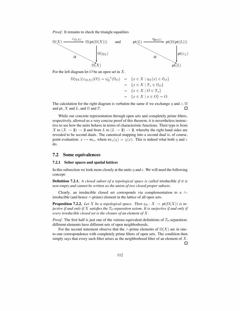
Proof. It remains to check the triangle equalities

#(X)0"(X)& #(pt(#(X))) and pt(L)

.pt(L)& pt(#(pt(L)))##########

id

?

##########id

?#(X)

#(.X)

'pt(L)

pt(0L)

'

For the left diagram let O be an open set inX .

#(.X)(0"(X)(O)) = .&1X (OO) = {x ! X | .X(x) ! OO}

= {x ! X | Fx ! OO}

= {x ! X | O ! Fx}

= {x ! X | x ! O} = O.

The calculation for the right diagram is verbatim the same if we exchange . and 0, #and pt, X and L, and O and F.

While our concrete representation through open sets and completely prime filters,respectively, allowed us a very concise proof of this theorem, it is nevertheless instruc-tive to see how the units behave in terms of characteristic functions. Their type is fromX to (X " 2) " 2 and from L to (L " 2) " 2, whereby the right hand sides arerevealed to be second duals. The canonical mapping into a second dual is, of course,point evaluation: x 9" evx, where evx(/) = /(x). This is indeed what both . and 0do.

7.2 Some equivalences7.2.1 Sober spaces and spatial lattices

In this subsection we look more closely at the units . and '. We will need the followingconcept:

Definition 7.2.1. A closed subset of a topological space is called irreducible if it isnon-empty and cannot be written as the union of two closed proper subsets.

Clearly, an irreducible closed set corresponds via complementation to a '-irreducible (and hence '-prime) element in the lattice of all open sets.

Proposition 7.2.2. Let X be a topological space. Then .X : X " pt(#(X)) is in-jective if and only if X satisfies the T0-separation axiom. It is surjective if and only ifevery irreducible closed set is the closure of an element ofX .

Proof. The first half is just one of the various equivalent definitions of T0-separation:different elements have different sets of open neighborhoods.

For the second statement observe that the '-prime elements of #(X) are in one-to-one correspondence with completely prime filters of open sets. The condition thensimply says that every such filter arises as the neighborhood filter of an element of X .

112

Definition 7.2.3. A topological space X is called sober if .X is bijective.

Note that if .X is bijective then it must be a homeomorphism because we knowfrom Section 7.1.4 that it is always continuous and open onto the image. By thepreceding proposition, a space is sober if and only if it is T0 and every irreducibleclosed set is the closure of a point. The intuitive meaning is, of course, that a space issober if it can be recovered from its lattice of open sets.

Proposition 7.2.4. For any complete latticeL the unit 0L : L " #(pt(L)) is surjectiveand monotone. Furthermore, the following are equivalent:

1. 0L is injective.

2. The elements of L are separated by completely prime filters.

3. L is '-generated by '-prime elements.

4. If x 8) y then there exists a completely prime filterF such that x ! F and y 8! F .

5. 0L is order-reflecting.

Proof. We have seen in Proposition 7.1.13 that all open sets on pt(L) are of the formOx for some x ! L. This proves surjectivity. Monotonicity is clear because filters areupper sets.

Turning to the equivalent conditions for injectivity, we note that Ox = Oy is equiv-alent to x ! F H( y ! F for all completely prime filters F . In other words, 0Lis injective if and only if the elements of L are separated by completely prime filters.Given x ! L let x% be the infimum of all '-primes above x. We want to show thatx = x%. If x% is strictly above x then there exists a completely prime filter contain-ing x% but not x. Using the equivalence of Proposition 7.1.11, we see that this is thesame as the existence of a '-prime element in /x \ /x%, a contradiction. From (3) thelast two statements follow easily. They, in turn, imply injectivity (which, in a generalorder-theoretic setting, is strictly weaker than order-reflection).

Definition 7.2.5. A complete lattice L is called spatial if 0L is bijective.

The intuitive meaning in this case is that a spatial lattice can be thought of as alattice of open sets for some topological space. A direct consequence of Theorem 7.1.8is the following:

Theorem 7.2.6. A spatial lattice is a frame. In particular, it is distributive.

Theorem 7.2.7. For any complete lattice L the topological space pt(L) is sober. Forany topological spaceX the lattice #(X) is spatial.

Proof. The space of points of a lattice L is certainly T0, because if we are given dif-ferent completely prime filters then there is x ! L which belongs to one of them butnot the other. Hence, Ox contains one but not the other. For surjectivity of .pt(L) letA be an irreducible closed set of filters. First of all, the union A of all filters in A is anon-empty upper set in L which is unreachable by joins. Hence the complement of A

113

is a principal ideal 0x. Also, the complement of A in pt(L) certainly contains Ox. Weclaim that x must be '-prime. Indeed, if y ' z ) x then A is covered by the comple-ments of Oy and Oz , whence it is covered by one of them, say the complement of Oy,which means nothing else than y ) x. It follows that A is contained in the closure ofthe point L \ 0x. On the other hand, L \ 0x belongs to the closed set A as each of itsopen neighborhoods contains an element of A.

The second statement is rather easier to argue for. If O and O% are different opensets then there is an element x of X contained in one but not the other. Hence theneighborhood filter of x, which is always completely prime, separates O and O%.

Corollary 7.2.8. The functors # and pt form a dual equivalence between the categoryof sober spaces and the category of spatial lattices.

This result may suggest that a reasonable universe of topological spaces ought toconsist of sober spaces, or, if one prefers the lattice-theoretic side, of spatial lattices.This is indeed true as far as spaces are concerned. For the lattice side, however, ithas been argued forcefully that the right choice is the larger category of frames (whichare defined to be those complete lattices which satisfy the frame distributivity law,Section 7.1.1). The basis of these arguments is the fact that free frames exist, see[Joh82], Theorem II.1.2, a property which holds neither for complete lattices nor forspatial lattices. (More information on this is in [Isb72, Joh82, Joh83].) The choiceof using frames for doing topology has more recently found support from theoreticalcomputer science, because it is precisely the frame distributivity law which can beexpected to hold for observable properties of processes. Even though this connectionis to a large extent the raison d’etre for this chapter, we must refer to [Abr87, Abr91b,Vic89, Smy92] for an in-depth discussion.

7.2.2 Properties of sober spaces

Because application of pt 5 # to a space X is an essentially idempotent operation, itis best to think of pt(#(X)) as a completion of X . It is commonly called the soberifi-cation of X . Completeness of this particular kind is also at the heart of the Hofmann-Mislove Theorem, which we have met in Section 4.2.3 already and which we are nowable to state in its full generality.

Theorem 7.2.9. Let X be a sober space. The sets of open neighborhoods of compactsaturated sets are precisely the Scott-open filters in #(X).

Proof. It is pretty obvious that the neighborhoods of compact subsets are Scott-openfilters in #(X). We are interested in the other direction. Given a Scott-open fil-ter F 1 #(X) then the candidate for the corresponding compact set is K =

#

F.We must show that each open neighborhood of K belongs to F already. For the sakeof contradiction assume that there exists an open neighborhood O 8! F. By Zorn’sLemma we may further assume that O is maximal with this property. Because F isa filter, O is '-prime as an element of #(X) and this is tantamount to saying that itscomplement A is irreducible as a closed set. By sobriety it must be the closure of asingle point x ! X . The open sets which do not contain x are precisely those which

114

are contained in O. Hence every open set from the filter F contains x and so x belongstoK . This, finally, contradicts our assumption that O is a neighborhood ofK .

This appeared first in [HM81]. Our proof is taken from [KP94]. Note that it relies,like almost everything else in this chapter, on the Axiom of Choice.

Saturated sets are uniquely determined by their open neighborhoods, so we canreformulate the preceding theorem as follows:

Corollary 7.2.10. Let X be a sober space. The poset of compact saturated sets or-dered by inclusion is dually isomorphic to the poset of Scott-open filters in #(X) (alsoordered by inclusion).

Corollary 7.2.11. Let X be a sober space. The filtered intersection of a family of(non-empty) compact saturated subsets is compact (and non-empty). If such a filteredintersection is contained in an open set O then some element of the family belongs toO already.

Proof. By the Hofmann-MisloveTheoremwe can switch freely between compact satu-rated sets and open filters in #(X). Clearly, the directed union of open filters is anothersuch. This proves the first statement. For the intersection of a filtered family to be con-tained in O means that O belongs to the directed union of the corresponding filters.Then O must be contained in one of these already. The claim about the intersection ofnon-empty sets follows from this directly because we can take O = B.

Every T0-space can be equipped with an order relation, called the specializationorder, by setting x & y if for all open sets O, x ! O implies y ! O. We may thencompare the given topology with topologies defined on ordered sets. One of thesewhich plays a role in this context, is the weak upper topology. It is defined as thecoarsest topology for which all sets of the form 0x are closed.

Proposition 7.2.12. For an T0-spaceX the topology onX is finer than the weak uppertopology derived from the specialization order.

Proposition 7.2.13. A sober space is a dcpo in its specialization order and its topologyis coarser than the Scott-topology derived from this order.

Proof. By the equivalence between sober spaces and spatial lattices we may think ofX as the points of a complete lattice L. It is seen without difficulties that the special-ization order on X then translates to the inclusion order of completely prime filters.That a directed union of completely prime filters is again a completely prime filter isimmediate.

Let!

#i"I Fi be such a directed union. It belongs to an open set Ox if and only if

x ! Fi for some i ! I . This shows that each Ox is Scott-open.

A dcpo equipped with the Scott-topology, on the other hand, is not necessarilysober, see Exercise 7.3.19(7). We also record the following fact although we shall notmake use of it.

Theorem 7.2.14. The category of sober spaces is complete and cocomplete. It is alsoclosed under retracts formed in the ambient category Top.

115

For the reader’s convenience we sum up our considerations in a table comparingconcepts in topological spaces to concepts in pt(L) for L a complete lattice.

space pt(L)

point completely prime filter (c. p. filter)specialization order inclusion order

open set c. p. filters containing some x ! Lsaturated set c. p. filters containing some upper set

compact saturated set c. p. filters containing a Scott-open filter

7.2.3 Locally compact spaces and continuous lattices

We already know that sober spaces may be seen as dcpo’s with an order-consistenttopology. We move on to more special kinds of spaces with the aim to characterize ourvarious kinds of domains through their open-set lattices. Our first step in this directionis to introduce local compactness. We have:

Lemma 7.2.15. Distributive continuous lattices are spatial.

Proof. We have shown in Theorem 7.1.7 that continuous lattices are '-generated by'-irreducible elements. In a distributive lattice these are also '-prime.

Now recall that a topological space is called locally compact if every element hasa fundamental system of compact neighborhoods. This alone does not imply sobriety,as the ascending chain of natural numbers, equipped with the weak upper topology,shows. But in combination with sobriety we get the following beautiful result:

Theorem 7.2.16. The functors # and pt restrict to a dual equivalence between thecategory of sober locally compact spaces and the category of distributive continuouslattices.

Proof. We have seen in Section 4.2.3 already that O : O% holds in #(X) if thereis a compact set between O and O%. This proves that the open-set lattice of a locallycompact space is continuous.

For the converse, let F be a point in an open set Ox, that is, x ! F . A completelyprime filter is Scott-open, therefore there is a further element y ! F with y : x.Lemma 2.3.8 tells us that there is a Scott-open filter G contained in //y which con-tains x. We know by the previous lemma that a distributive continuous lattice can bethought of as the open-set lattice of its space of points, which, furthermore, is guaran-teed to be sober. So we can apply the Hofmann-Mislove Theorem 7.2.9 and get thatthe set A of points of L, which are supersets of G, is compact saturated. In summary,F is contained in Oy which is a subset ofA and this is a subset of Ox.

From now on, all our spaces are locally compact and sober. The three propertiesintroduced in the next three subsections, however, are independent of each other.

116

7.2.4 Coherence

We have introduced coherence in Section 4.2.3 for the special case of continuous do-mains. The general definition reads as follows:

Definition 7.2.17. A topological space is called coherent, if it is sober, locally compact,and the intersection of two compact saturated subsets is compact.

Definition 7.2.18. The order of approximation on a complete lattice is called multi-plicative if x : y and x : z imply x : y ' z. A distributive continuous lattice forwhich the order of approximation is multiplicative is called arithmetic.

As a generalization of Proposition 4.2.16 we have:

Theorem 7.2.19. The functors # and pt restrict to a dual equivalence between thecategory of coherent spaces and the category of arithmetic lattices.

Proof. The same arguments as in Proposition 4.2.15 apply, so it is clear that the open-set lattice of a coherent space is arithmetic. For the converse we may, just as in theproof of Theorem 7.2.16, invoke the Hofmann-Mislove Theorem. It tells us that com-pact saturated sets of pt(L) are in one-to-one correspondence with Scott-open filters.Multiplicativity of the order of approximation is just what we need to prove that thepointwise infimum of two Scott-open filters is again Scott-open.

7.2.5 Compact-open sets and spectral spaces

By passing from continuous lattices to algebraic ones we get:

Theorem 7.2.20. The functors # and pt restrict to a dual equivalence between thecategory of sober spaces, in which every element has a fundamental system of compact-open neighborhoods, and the category of distributive algebraic lattices.

The proof is the same as for distributive continuous lattices, Theorem 7.2.16. Wenow combine this with coherence.

Definition 7.2.21. A topological space, which is coherent and in which every elementhas a fundamental system of compact-open neighborhoods, is called a spectral space.

Theorem 7.2.22. The functors # and pt restrict to a dual equivalence between thecategory of spectral spaces and the category of algebraic arithmetic lattices.

Having arrived at this level, we can replace the open-set lattice with the sublatticeof compact-open subsets. Our next task then is to reformulate Stone-duality with basesof open-set lattices. For objects we have:

Proposition 7.2.23. Let L be an algebraic arithmetic lattice. The completely prime fil-ters of L are in one-to-one correspondence with the prime filters ofK(L). The topologyon pt(L) is generated by the set of all Ox, where x is compact in L.

117

Proof. Given a completely prime filter F in L, we let F * K(L) be the set of compactelements contained in it. This is clearly an upwards closed set in K(L). It is a filter,because L is arithmetic. Primeness, finally, follows from the fact that F is Scott-openand hence equal to /(F * K(L)). Conversely, a filter G in K(L) generates a filter /Gin L. For complete primeness let A be a subset of L with join in /G. L is algebraic.So we may replace A by B = 0A * K(L) and

/

B ! /G will still hold. Because /Gis Scott-open, there is a finite subset M of B with

/

M ! /G. Some element of Gmust be below

/

M and primeness then gives us that some element ofM belongs toGalready.

The statement about the topology on pt(L) follows from the fact that every elementof L is a join of compact elements.

A frame-homomorphism between algebraic arithmetic lattices need not preservecompact elements, so in order to represent it through bases we need to resort to re-lations, as in Section 2.2.6, Definition 2.2.27. Two additional axioms are needed,however, because frame-homomorphisms are more special than Scott-continuous func-tions.

Definition 7.2.24. A relationR between lattices V andW is called join-approximableif the following conditions are satisfied:

1. >x, x% ! V >y, y% ! W. (x% 4 x R y 4 y% =( x% R y%);

2. >x ! V >N 1fin W. (>y ! N. x R y =( x R (/

N));

3. >M 1fin V >y ! W. (>x ! M. x R y =( (0

M) R y);

4. >M 1fin V >x ! W. ((/

M) R x =( ?N 1fin W.(x =

/

N ' >n ! N?m ! M. m R n)).

The following is then easily established:

Proposition 7.2.25. The category of algebraic arithmetic lattices and frame-homomorphisms is equivalent to the category of distributive lattices and join-approximable relations.

By Proposition 7.2.23 we can replace the compound functor pt 5 Idl by a directconstruction of a topological space out of a distributive lattice. We denote this functorby spec, standing for the spectrum of a distributive lattice. We also contract K 5 # toK#. Then we can say:

Theorem 7.2.26. The category of spectral spaces and continuous functions is duallyequivalent to the category of distributive lattices and join-approximable relations viathe contravariant functors K# and spec.

We supplement the table in Section 7.2.2 with the following comparison of con-cepts in a topological space and concepts in the spectrum of a distributive lattice.

118

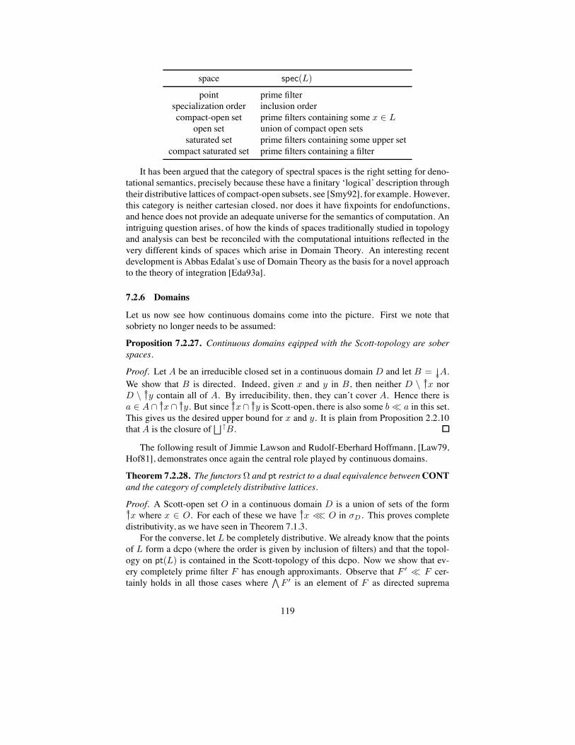
space spec(L)

point prime filterspecialization order inclusion ordercompact-open set prime filters containing some x ! L

open set union of compact open setssaturated set prime filters containing some upper set

compact saturated set prime filters containing a filter

It has been argued that the category of spectral spaces is the right setting for deno-tational semantics, precisely because these have a finitary ‘logical’ description throughtheir distributive lattices of compact-open subsets, see [Smy92], for example. However,this category is neither cartesian closed, nor does it have fixpoints for endofunctions,and hence does not provide an adequate universe for the semantics of computation. Anintriguing question arises, of how the kinds of spaces traditionally studied in topologyand analysis can best be reconciled with the computational intuitions reflected in thevery different kinds of spaces which arise in Domain Theory. An interesting recentdevelopment is Abbas Edalat’s use of Domain Theory as the basis for a novel approachto the theory of integration [Eda93a].

7.2.6 Domains

Let us now see how continuous domains come into the picture. First we note thatsobriety no longer needs to be assumed:

Proposition 7.2.27. Continuous domains eqipped with the Scott-topology are soberspaces.

Proof. Let A be an irreducible closed set in a continuous domain D and let B = 00A.We show that B is directed. Indeed, given x and y in B, then neither D \ //x norD \ //y contain all of A. By irreducibility, then, they can’t cover A. Hence there isa ! A* //x* //y. But since //x* //y is Scott-open, there is also some b : a in this set.This gives us the desired upper bound for x and y. It is plain from Proposition 2.2.10that A is the closure of

"

#B.

The following result of Jimmie Lawson and Rudolf-Eberhard Hoffmann, [Law79,Hof81], demonstrates once again the central role played by continuous domains.

Theorem 7.2.28. The functors# and pt restrict to a dual equivalence betweenCONTand the category of completely distributive lattices.

Proof. A Scott-open set O in a continuous domain D is a union of sets of the form//x where x ! O. For each of these we have //x % O in )D . This proves completedistributivity, as we have seen in Theorem 7.1.3.

For the converse, let L be completely distributive. We already know that the pointsof L form a dcpo (where the order is given by inclusion of filters) and that the topol-ogy on pt(L) is contained in the Scott-topology of this dcpo. Now we show that ev-ery completely prime filter F has enough approximants. Observe that F % : F cer-tainly holds in all those cases where

0

F % is an element of F as directed suprema

119

of points are unions of filters. Now given x ! F we get from prime-continuitythat x =

/

{y | y % x} and so there must be some y ! F with y % x. Suc-cessively interpolating between y and x gives us a sequence of elements such thaty % . . . % yn % . . . % y1 % x, just as in the proof of Lemma 2.3.8. Theset

!

n"N/yn then is a completely prime filter containing x with infimum in F . The

directedness of these approximants is clear because F is filtered. As a consequence,we have that F % : F holds if and only if

0

F % belongs to F .We are not quite finished, though, because we also need to show that we get the

Scott-topology back. To this end let O be a Scott-open set of points, that is, F < F % !O implies F ! O and

!

#i"I Fi ! O implies Fi ! O for some i ! I . Let x be the

supremum of all elements of the form0

F , F ! O. We claim that O = Ox. First ofall, for each F ! O there is F % ! O with F % : F , which, as we have just seen, istantamount to

0

F % ! F , hence x belongs to all F and O 1 Ox is proved.Conversely, if a pointG contains x then it must contain some

0

F , F ! O, becauseit is completely prime. HenceG belongs to O, too, and we have shown Ox 1 O.

To this we can add coherence and we get a dual equivalence between coherentdomains and completely distributive arithmetic lattices. Or we can add algebraicity andget a dual equivalence between algebraic domains and algebraic completely distributivelattices. Adding both properties characterizes what can be called 2/3-bifinite domainsin the light of Proposition 4.2.17. We prefer to speak of coherent algebraic domains.As these are spectral spaces, we may also ask how they can be characterized throughthe lattice of compact open subsets. The answer is rather simple: A compact open setin an algebraic domain D is a finite union of sets of the form /c for c ! K(D). These,in turn, are characterized by being G-irreducible and also G-prime.

Theorem 7.2.29. The dual equivalence of Theorem 7.2.26 cuts down to a dual equiv-alence of coherent algebraic domains and lattices in which every element is the join offinitely many G-primes.

Proof. We only need to show that if a lattice satisfies the condition stated in the theo-rem, then its ideal completion is completely distributive. But this is trivial because aprincipal ideal generated by a G-prime is completely G-prime in the ideal completionand so the result follows from Theorem 7.1.3.

All the combined strength of complete distributivity, algebraicity and multiplica-tivity of the order of approximation, however, does still not restrict the correspondingspaces far enough so as to bring us into one of our cartesian closed categories of do-mains. Let us therefore see what we have to add in order to characterize bifinite do-mains. The only solution in this setting appears to be a translation of mub-closuresinto the lattice of compact-open subsets, that is to say, the subset of G-primes has theupside-down finite mub property (Definition 4.2.1). Let us sum up these considerationsin a theorem:

Theorem 7.2.30. A lattice V is isomorphic to the lattice of compact-open subsets ofan F-B-domain (Definition 4.3.7) if and only if, firstly, V has a least element, secondly,

120

each element of V is the supremum of finitely many G-primes and, thirdly, for everyfinite set M of G-primes there is a finite superset N of G-primes such that

>A 1 M ?B 1 N.-

A =.

B.

The additional requirement that there be a largest element which is also G-prime, char-acterizes the lattices of compact-open subsets of bifinite domains.

The extra condition about finite mub-closures is not a first-order axiom and cannotbe replaced by one as was shown by Carl Gunter in [Gun86]. The smaller class ofalgebraic bc-domains has a rather nicer description:

Theorem 7.2.31. A lattice V is isomorphic to the lattice of compact-open subsets ofan algebraic bc-domain if and only if it has a least element, each element of V is thesupremum of finitely manyG-primes and the set ofG-primes plus least element is closedunder finite infima.

7.2.7 Summary

We have summarized the results of this section in Figure 16 and Table 1. As labelswe have invented a few mnemonic names for categories. We won’t use them outsidethis subsection. The filled dots correspond to categories for which there is also a char-acterization in terms of compact-open subsets (spectral spaces). A similar diagramappears in [GHK+80] but there not everything, which appears to be an intersection ofcategories, really is one.

7.3 The logical viewpointThis material is based on [Abr91b].

7.3.1 Working with lattices of compact-open subsets

Having established the duality between algebraic domains and their lattices ofcompact-open subsets we can now ask to what extent we can do domain theory throughthese lattices. We have already indicated that such an approach offers many new in-sights but for the moment our motivation could simply be that working with lattices isa lot easier than working with dcpo’s. ‘Doing domain theory’ refers to performing thedomain constructions of Sections 3.2, 3.3, 5 and 6, at least in a first approximation.

Let us try this out. Suppose you know K#(D) for some bifinite domainD, how doyou construct K#(D$), the lattice of compact-open subsets of the lifted domain? Theanswer is simple, just add a new top element: K#(D$) = K#(D)9. Coalesced sumalso works fine:

K#(D C E) = (K#(D) \ {D}) % (K#(E) \ {E}) 6 {D C E}.

We encounter the first problemswhen we look at the cartesian product. While it is clearthat every compact-open subset ofD%E is a finite union of products of compact-open

121

TOP Topological spaces. No Stone-dual.

SOB Sober spaces vs. spatial lattices.

L-C Locally-compact sober spaces vs. continuous distributivelattices.

COH Coherent spaces (= locally compact, sober, and intersection ofcompact saturated is compact) vs. arithmetic lattices (= distribu-tive, continuous, and order of approximation is multiplicative).

C-O Sober spaces with a base of compact-open sets vs. distributivealgebraic lattices.

CONT Continuous domains with Scott-topology vs. completely dis-tributive lattices.

SPEC Spectral spaces vs. algebraic arithmetic lattices vs. distributivelattices.

C-CONT Coherent domains vs. arithmetic completely distributive lattices.

ALG Algebraic domains vs. algebraic completely distributive lattices.

C-ALG Coherent algebraic domains vs. algebraic arithmetic completelydistributive lattices vs. distributive lattices in which every ele-ment is the finite join of G-primes.

F-B F-B-domains (Definition 4.3.7) (= bilimits of finite posets).Stone-dual only described through the basis (or base) ofcompact-open subsets, which is a distributive lattice with extraproperties as stated in Theorem 7.2.30.

B Bifinite domains. Stone-dual only described through the basis ofcompact-open subsets, which is a distributive lattice with extraproperties as stated in Theorem 7.2.30.

aBC Algebraic bounded-complete domains. Stone-dual only de-scribed through the basis of compact-open subsets, which isa distributive lattice with extra properties as stated in Theo-rem 7.2.31.

Table 1: The categories and their Stone-duals.

122

- aBC- B- F-B- C-ALG

-SPEC ' C-CONT ' ALG

'COH ' C-O ' CONT

' L-C' SOB' TOP""""

++

++

++

+++.

..

..

..

.. ++

++

++

+++.

..

..

..

..

++

++

++

+++.

..

..

..

.. ++

++

++

+++.

..

..

..

..

Figure 16: An overview of Stone-dualities in domain theory.

subsets in the factors, there seems to be no simple criterion on such unions which wouldguarantee unique representation.

The moral then is that we must allow for multiple representations of compact-opensubsets. Instead of lattices we shall study certain preordered structures. At first glancethis may seem as an unwanted complication but we will soon see that it really makesthe whole programme work much more smoothly.

Lattices are determined by either their order structure or their algebraic structurebut this equivalence no longer holds in the preordered case. Instead we must mentionboth preorder and lattice operations. We also make G-primeness explicit in our axiom-atization. The reason for this is that we want to keep all our definitions inductive. Thispoint will become clearer when we discuss the function space construction below.

Definition 7.3.1. A coherent algebraic prelocale A is a preordered algebra with two

123

binary operations G and ', two nullary operations 0 and 1, and a unary predicate Con A, such that a G b is a supremum for {a, b}, a ' b is an infimum for {a, b}, 0 is aleast, and 1 is a largest element. The preorder onA is denoted by&, the correspondingequivalence relation by F. The predicate C(a) is required to hold if and only if a isG-prime. Finally, every element of A must be equivalent to a finite join of G-primes.

We will not distinguish between a prelocale and its underlying set. The set{a ! A | C(a)} is abbreviated as C(A).

This is essentially the definition which appears in [Abr91b]. There another pred-icate is included. We can omit this because we will not look at the coalesced sumconstruction. The expressions ‘a supremum’, ‘an infimum’, etc., may seem contra-dictory but they are exactly appropriate in the preordered universe. It is seen withoutdifficulties that every coherent algebraic prelocale A gives rise to a lattice A/2 whichis G-generated by G-primes and hence distributive.

A domain prelocale is gotten by incorporating the two extra conditions from The-orem 7.2.30:

• >u 1fin C(A) ?v 1fin C(A). u 1 v and (>w 1 u ?z 1 v.0

w =/

z);

• C(1).

Definition 7.3.2. Let A and B be domain prelocales. A function % : A " B is calleda pre-isomorphism if it is surjective, order-preserving and order-reflecting. If A is adomain prelocale and D is a bifinite domain and if further there is a pre-isomorphism#·$ : A " K#(D) then we say that A is a localic description of D via #·$.

A pre-isomorphism % : A " B must preserve suprema, infima, and least andlargest element (up to equivalence). Furthermore, it restricts and corestricts to a surjec-tive map %0 : C(A) " C(B). Let us lookmore closely at the case of a pre-isomorphism#·$ : A " K#(D). A diagram may be quite helpful:

C(A) & & A

K(D) $=dual C(K#(D))

#·$0

'& & K#(D)

#·$

'

Remember that C(K#(D)) are just those compact-open subsets which are of theform /c for c ! K(D). The inclusion order between such principal filters is dual to theusual order on K(D).

Let us now lift the pre-isomorphism to the domain level. In the previous chapters,the natural approach would have been to apply the ideal completion functor to the pre-isomorphism between C(A)op and K(D). Here we use Stone-duality and apply specto #·$. This yields an isomorphism between spec(A) and spec(K#(D)). Composed

124

with the inverse of the unit . it gives us the isomorphism - : spec(A) " D.

spec(A)##########

-

?spec(K#(D))

spec(#·$)&1

' .&1& D

It will be good to have a concrete idea of the behaviour of - , at least for compactelements of spec(A). These are filters in A which are generated by G-prime elements.So let F = /a with a ! C(A). It is easily checked that -(F ) equals that compactelement c ofD which is least in the compact-open subset #a$0.

Proposition 7.3.3. There exists a map #·$ : A " K#(D) such that the domain prelo-cale A is a localic description of the bifinite domain D if and only if spec(A) and Dare isomorphic.

Proof. We have just described how to derive an isomorphism from a pre-isomorphism.For the converse observe that the unit 0 : A " K#(spec(A)) is surjective, order-preserving and order-reflecting (Proposition 7.2.4).

For more general functions between domains, we can translate join-approximablerelations into the language of domain prelocales. The following is then just a slightextension of Theorem 7.2.30.

Theorem 7.3.4. The category of domain prelocales and join-approximable relationsis dually equivalent to the category of bifinite domains and Scott-continuous functions.

Our attempt to mimic the cartesian product construction forced us to pass to pre-ordered structures but once we have accepted this we can go one step farther and makethe prelocales syntactic objects in which no identifications are made at all. More pre-cisely, it is no loss of generality to assume that the underlying algebra is a term algebrawith respect to the operations G,', 0, and 1. As an example, let us describe the one-point domain I in this fashion. We take the term algebra on no generators, that is, everyterm is a combination of 0’s and 1’s. The preorder is the smallest relation compatiblewith the requirements in Definition 7.3.1. The effect of this is that there are exactly twoequivalence classes with respect to F, the terms equivalent to 1 and the terms equiva-lent to 0. The former are precisely the G-prime terms. We denote the resulting domainprelocale by 1.

The syntactic approach also suggests that we look at the following relation betweendomain prelocales:

Definition 7.3.5. Let A and B be domain prelocales. We say that A is a sub-prelocaleof B if the following conditions are satisfied:

1. A is a subalgebra of B with respect to G,', 0 and 1.

2. The preorder on A is the restriction of the preorder on B to A.

125

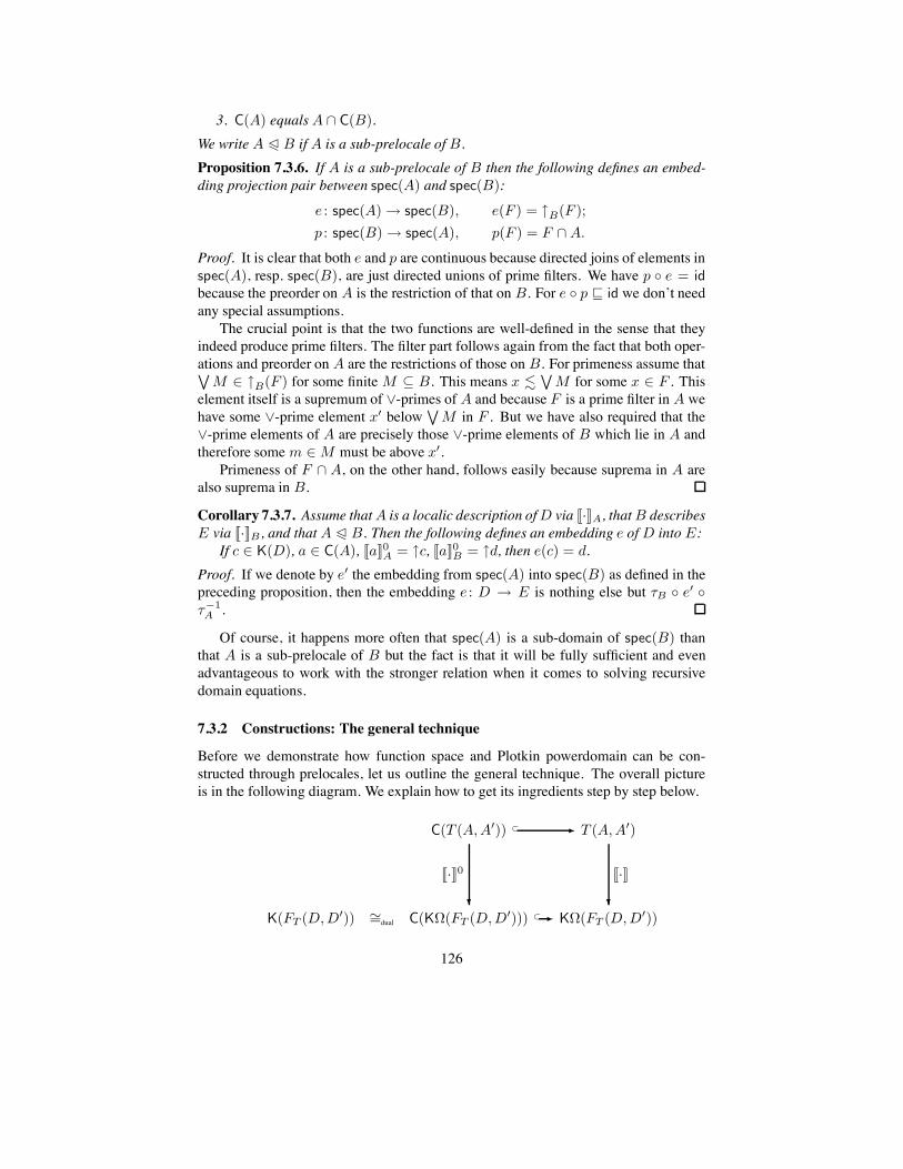
3. C(A) equalsA * C(B).We write A % B if A is a sub-prelocale of B.Proposition 7.3.6. If A is a sub-prelocale of B then the following defines an embed-ding projection pair between spec(A) and spec(B):

e : spec(A) " spec(B), e(F ) = /B(F );

p : spec(B) " spec(A), p(F ) = F * A.

Proof. It is clear that both e and p are continuous because directed joins of elements inspec(A), resp. spec(B), are just directed unions of prime filters. We have p 5 e = idbecause the preorder on A is the restriction of that on B. For e 5 p & id we don’t needany special assumptions.

The crucial point is that the two functions are well-defined in the sense that theyindeed produce prime filters. The filter part follows again from the fact that both oper-ations and preorder on A are the restrictions of those on B. For primeness assume that/

M ! /B(F ) for some finite M 1 B. This means x &/

M for some x ! F . Thiselement itself is a supremum of G-primes of A and because F is a prime filter in A wehave some G-prime element x% below

/

M in F . But we have also required that theG-prime elements of A are precisely those G-prime elements of B which lie in A andtherefore somem ! M must be above x%.

Primeness of F * A, on the other hand, follows easily because suprema in A arealso suprema in B.

Corollary 7.3.7. Assume thatA is a localic description ofD via #·$A, thatB describesE via #·$B , and that A % B. Then the following defines an embedding e of D into E:

If c ! K(D), a ! C(A), #a$0A = /c, #a$0B = /d, then e(c) = d.Proof. If we denote by e% the embedding from spec(A) into spec(B) as defined in thepreceding proposition, then the embedding e : D " E is nothing else but -B 5 e% 5-&1A .

Of course, it happens more often that spec(A) is a sub-domain of spec(B) thanthat A is a sub-prelocale of B but the fact is that it will be fully sufficient and evenadvantageous to work with the stronger relation when it comes to solving recursivedomain equations.

7.3.2 Constructions: The general technique

Before we demonstrate how function space and Plotkin powerdomain can be con-structed through prelocales, let us outline the general technique. The overall pictureis in the following diagram. We explain how to get its ingredients step by step below.

C(T (A, A%)) & & T (A, A%)

K(FT (D, D%)) $=dual C(K#(FT (D, D%)))

#·$0

'&& K#(FT (D, D%))

#·$

'

126

1. The set-up. We want to study a construction T on (bifinite) domains. Thiscould be any one from the table in Section 3.2.6 or a bilimit or one of the powerdomainconstructions from Section 6.2. The diagram illustrates a binary construction. We canassume that we understand the action of the associated functor FT on bifinite domains.In particular, we knowwhat the compact elements ofFT (D, D%) are, how they compareand how FT acts on embeddings (Proposition 5.2.6). Thus we should have a clearunderstanding of the bottom row of the diagram, in detail:

• FT (D, D%) is the effect of the functor FT on objectsD andD%.

• K(FT (D, D%)) are the compact elements of FT (D, D%).

• K#(FT (D, D%)) are the compact-open subsets of FT (D, D%) and these are pre-cisely those upper sets which are of the form /u for a finite set u of compactelements.

• C(K#(FT (D, D%))) are the G-prime elements of K#(FT (D, D%)) and these areprecisely those subsets of FT (D, D%) which are of the form /c for c a compactelement. The order is inclusion which is dual to the usual order on compactelements.

Furthermore, we assume that we are given domain prelocales A andA% which describethe bifinite domains D and D%, respectively. These descriptions are encoded in pre-isomorphisms #·$A : A " K#(D) and #·$A" : A% " K#(D%).2.The goal. We want to define a domain prelocale T (A, A%) which is a localic

description of FT (D, D%). This is achieved in the following series of steps.3. Definition of T (A, A%). This is the creative part of the enterprise. We search

for a description of compact-open subsets of FT (D, D%) based on our knowledge ofthe compact-open subsets of D and D%. The point is to do this directly, not via thecompact elements ofD,D%, and FT (D, D%). There will be an immediate payoff, as wewill gain an understanding of the construction in terms of properties rather than points.Our treatment of the Plotkin powerdomain below illustrates this most convincingly.

The definition of T (A, A%) will proceed uniformly in all concrete instances. Firsta set GT of generators is defined and then T (A, A%) is taken to be the term alge-bra over GT with respect to G,', 0, and 1. An interpretation function #·$ : GT "K#(FT (D, D%)) is defined based on the interpretations #·$A and #·$A" . It is extendedto all of T (A, A%) as a lattice homomorphism: #a G b$ = #a$6#b$, etc. Finally, axiomsand rules are given which govern the preorder and G-primeness predicate.

Next we have to check that our definitions work. This task is also broken into aseries of steps as follows.4. Soundness. We check that axioms and rules translate via #·$ into valid state-

ments about compact-open subsets of FT (D, D%). This is usually quite easy. Fromsoundness we infer that #·$ is monotone and can be restricted and corestricted to a map#·$0 : C(T (A, A%)) " C(K#(FT (D, D%))).5. Prime generation. Using the axioms and rules, we prove that every element

of T (A, A%) can be transformed (effectively) into an equivalent term which is a finitesupremum of expressions which are asserted to be G-prime. This is the crucial stepand usually contains the main technical work. It allows us to prove the remaining

127

properties of #·$ through #·$0 and for the latter we can use our knowledge of the basisof FT (D, D%).6. Completeness for G-primes. We show that #·$0 is order reflecting.7. Definability for G-primes. We show that #·$0 is surjective.At this point we can fill in the remaining pieces without reference to the concrete

construction under consideration.8. Completeness. The interpretation function #·$ itself is order-reflecting.

Proof. Let a, b ! T (A, A%) be such that #a$ 1 #b$. By 5 we can replace these ex-pressions by formal joins of G-primes: a F a1 G . . . G an and b F b1 G . . . G bm.Soundness ensures that the value under the interpretation function remains unchangedand that each #ai$ (resp. #bj$) is of the form /ci (resp. /dj) for ci, dj compact elementsin FT (D, D%). The inclusion order on K#(FT (D, D%)) translates into the formula>i ?j. /ci 1 /dj which by the completeness for G-primes can be pulled back intoT (A, A%): >i ?j. ai & bj . In every preordered lattice it must follow that a & bholds.

9. Definability. The surjectivity of #·$ is an easy consequence of the surjectivityof #·$0 because we know that compact-open subsets in an algebraic domain are finiteunions of compactly generated principal filters.10. Well-definedness. Of course, K#(FT (D, D%)) is a domain prelocale and we

have just shown that preorder and primeness predicate on T (A, A%) are preserved andreflected by #·$. This constitutes a semantic proof that T (A, A%) satisfies the two extraconditions for domain prelocales. In other words, T is a well-defined operation ondomain prelocales.11. Stone-duality. At this point we have shown that #·$ is a pre-isomorphism. As

in the previous subsection we lift it to an isomorphism - between spec(T (A, A%)) andFT (D, D%) via Stone duality:

spec(T (A, A%))##########

-

?spec(K#(FT (D, D%)))

spec(#·$)&1

' .&1& FT (D, D%)

So much for the correspondence on the object level. We also want to see howthe construction T harmonizes with the sub-prelocale relation, one the one hand,and the isomorphism - , on the other hand. Thus we assume that we are giventwo more prelocales, B and B%, which are localic descriptions of bifinite domainsE and E%, such that A % B and A% % B% hold. In Corollary 7.3.7 we have seenhow to define from this embeddings e : D " E and e% : D% " E%. In Proposi-tion 5.2.6 we have shown how the functors associated with different constructionsact on embeddings, hence we may unambiguously write FT (e, e%) for the result ofthis action, which is an embedding from FT (D, D%) to FT (E, E%). Embeddings pre-serve compact elements so FT (e, e%) restricts and corestricts to a monotone functionFT (e, e%)0 : K(FT (D, D%)) " K(FT (E, E%)). Now for both T (A, A%) and T (B, B%)

128

we have a diagram such as depicted at the beginning of this subsection. We connectthe lower left corners of these by FT (e, e%)0. This gives rise also to a map i fromC(K#(FT (D, D%))) to C(K#(FT (E, E%))). Our way of defining T (A, A%) will besuch that it is immediate that C(T (A, A%)) is a subset of C(T (B, B%)) and hence thereis an inclusion map connecting the upper left corners. Our next technical step then isthe following.12. Naturality.We show that the diagram

C(T (A, A%)) & & C(T (B, B%))

C(K#(FT (D, D%)))

#·$0T (A,A")

' i& C(K#(FT (E, E%)))

#·$0T (B,B")

'

commutes. On the element level this reads: If a ! C(T (A, A%)) and #a$0T (A,A") = /c

and #a$0T (B,B") = /d then FT (e, e%)0(c) = d. Now we can again get the remainingmissing information in a general manner.13. Monotonicity. We show that T (A, A%) % T (B, B%). From the form of our

construction it will be clear that T (A, A%) is a subset of T (B, B%) and the axioms andrules will be such that whatever can be derived in T (A, A%) can also be derived inT (B, B%). We must show that in the larger prelocale nothing extra can be proved forelements of T (A, A%). The argument is a semantic one.

Proof. Let a, a% ! C(T (A, A%)) such that a & a% holds in T (B, B%). Let #a$0T (A,A") =

/c, #a$0T (B,B") = /d and similarly for a%. Correctness says that /d 1 /d% and henced + d%. By naturality we have FT (e, e%)0(c) = d + d% = FT (e, e%)0(c%). Embeddingsare order reflecting so c + c% follows. Completeness then allows us to conclude thata & a% holds in T (A, A%) as well.

In the same way it is seen that the predicate C on T (A, A%) is the restriction of thaton T (B, B%).

14. Least prelocale. It follows from the correctness of the construction that 1 %T (A, A%) holds.15. Naturality of - . Having established the relation T (A, A%) % T (B, B%) we

can look at the embedding I : spec(T (A, A%)) " spec(T (B, B%)) which we defined inProposition 7.3.6. We claim that the following diagram commutes:

spec(T (A, A%))I & spec(T (B, B%))

FT (D, D%)

-A

' FT (e, e%)& FT (E, E%)

-B

'

In other words, FT (e, e%) equals the embedding which can be derived from T (A, A%) %T (B, B%) in the general manner of Corollary 7.3.7.

129

Proof. This is a diagram of bifinite domains and Scott-continuous functions. It there-fore suffices to check commutativity for compact elements. A compact element inspec(T (A, A%)) is a filter F generated by a term a ! C(T (A, A%)). Its image under -Ais the compact element c which generates the compact-open subset #a$0T (A,A"). Thefilter I(F ) is generated by the same term a. Applying -B to it gives us a compactelement d which is least in #a$0T (A,A"). Step 12 ensures that FT (e, e%) maps c to d.

7.3.3 The function space construction

We start out with two preparatory lemmas. The following notation will be helpful. Wewrite (A ( B) for the set of functions which map all of A into B.

Lemma 7.3.8. The Scott-topology on the function space [D #" D%] for bifinite do-mainsD andD% equals the compact-open topology.

Proof. Let A 1 D be compact and O 1 D% be open and let F 1 [D #" D%] be adirected set of continuous functions for which

"

#F maps A into O. For every x ! Awe have (

"

#F )(x) ! O and because O is open, there is fx ! F with fx(x) ! O. Thecollection of open sets of the form f&1

x (O), x ! A, covers A. By compactness, thisis true for finitely many f&1

x (O) already. If we let f be an upper bound in F for thesefx, then A 1 f&1(O) holds which is equivalent to f(A) 1 O. Hence (A ( O) is aScott-open set in [D #" D%].

If, on the other hand, f belongs to a Scott-open open set O 1 [D #" D%] thenthis is true also for some approximation g%m 5 f 5 gn with gn an idempotent deflationon D, g%m an idempotent deflation on D%. For each element x in the image of gn wehave the set (/x ( (//g%m 5 f 5 gn(x))). The intersection of all these belongs to thecompact-open topology, contains f , and is contained in O.

Lemma 7.3.9. LetD andD% be bifinite and letA 1 D andA% 1 D% be compact-open.Then (A ( A%) is compact-open in [D #" D%].

Proof. We know that (A ( A%) defines an open set by the previous lemma. Frombifiniteness we get idempotent deflations gn onD and g%m onD% such thatA = /gn(A)and A% = /g%m(A%). It follows that (A ( A%) = /Gnm(A ( A%) for the idempotentdeflationGnm on [D #" D%] which maps f to g%m 5 f 5 gn.

Now let A and A% be domain prelocales describing bifinite domains D and D%, asoutlined in the general scheme in the previous subsection. The two lemmas justifythe following choice of generators and interpretation function for our localic functionspace construction:

G5 = {(a " a%) | a ! A, a% ! A%};

#(a " a%)$ = (#a$A ( #a%$A")

Note that the elements (a " a%) are just syntactic expressions. Here are axiomsand rules for the preorder and C-predicate.

130

Axioms.(" # ') (a "

0

i"I a%i) F

0

i"I(a " a%i).

(" # G # l) (/

i"I ai " a%) F0

i"I(ai " a%).(dist) a ' (b G c) F (a ' b) G (a ' c).Rules.(" # G # r) If C(a) then (a "

/

i"I a%i) F

/

i"I(a " a%i).

(" # &) If b & a and a% & b% then (a " a%) & (b " b%).(" # C) If >i ! I. (C(ai) and C(a%

i)) and if >K 1 I ?L 1 I.(0

k"K ak F/

l"L al and (>k ! K, l ! L. a%k & a%

l)) thenC(

0

i"I(ai " a%i)).

A few comments about these formulae are in place. First a convention: we assumethat all index sets are finite, so that the expressions

0

i"I ai, etc., do indeed belong tothe term algebra overG5. Observe the use of the C-predicate in the rule (" # G # r).Without it, it would be very difficult to express this property. Also note that we enforcedistributivity. This will be a prerequisite to prove prime generation below.

It is clear that the rules are sound for the given interpretation, in particular, (" # C)is the exact mirror image of our definition of joinable families of step functions, Def-inition 4.2.2. Let us therefore immediately turn to the crucial step 5. We cannot useLemma 7.3.9 directly because we have not encoded the idempotent deflations. Wemust find the minimal elements of a compact-open subset explicitly. We illustrate thegeneral technique in an example.

Suppose #a$A is of the form /c 6 /d and #a%$A" is of the form /c% 6 /d%. We geta minimal element of ((/c 6 /d) ( (/c% 6 /d%)) by choosing a value f(c) and a valuef(d) from {c%, d%}. Then we must look at the intersection /c * /d which again is ofthe form /e1 6 . . . 6 /en by coherence. For each ei we must choose a value frommub{f(c), f(d)} = {e%1, . . . , e

%m}. And so on. Bifiniteness of the argument domain

ensures that this process stops after a finite number of iterations and that the result isa joinable family of pairs ,x, f(x)-. Coherence of the result domain guarantees thatall in all only finitely many choices are possible. (Note that it can happen that a set ofminimal upper bounds in the image domain is empty. In this case we have just beenunlucky with our choices. If #a%$A" is not empty then some minimal function exists.)

We can mimic this procedure in the prelocale as follows. For simplicity and to makethe analogy apparent, we let c, d stand for terms such that C(c), C(d) and a F c G d.Similarly for a%. We get:

(a " a%) FF ((c G d) " (c% G d%)) (" # &)F (c " (c% G d%)) ' (d " (c% G d%)) (" # G # l)F ((c " c%) G (c " d%)) ' ((d " c%) G (d " d%)) (" # G # r)F ((c " c%) ' (d " d%)) G . . . (3 more terms) (dist)

We follow up only the first of these four terms. The trick is to smuggle in the G-prime

131

terms e1, . . . , en whose join equals c ' d.

(c " c%) ' (d " d%) FF ((c G e1 G . . . G en) " c%) ' ((d G e1 G . . . G en) " d%) (" # &)F (c " c%) ' (d " d%) ' ((e1 G . . . G en) " (c% ' d%)) (" # G # l)F (c " c%) ' (d " d%) ' ((e1 G . . . G en) " (e%1 G . . . G e%m))

and now induction may do its job. Eventually we will have transformed (a " a%)into a disjunction of joinable families. For these, G-primeness may be inferred throughrule (" # C). Note that distributivity allows us to replace every term by an equivalentterm of the form

/

(0

(ai " a%i)) and for each term of the form

0

(ai " a%i) the

transformation works as illustrated.Next we show completeness for G-primes. So assume a and b are terms for which

the C-predicate holds and for which #a$ 1 #b$. It must be the case that a and b areequivalent to joinable families

0

i"I(ai " a%i) and

0

j"J (bj " b%j) as there is noother way of deriving G-primeness in [A #" A%]. The order relation between joinablefamilies has been characterized in Lemma 4.2.3. Here it says: >i ! I ?j ! J. (#bj$ 1#ai$ and #a%

i$ 1 #b%j$). Since we assume completeness for the constituting prelocalesA and A%, we may infer >i ! I ?j ! J. (bj & ai and a%

i & b%j). The relation a & b isnow easily derived from (" # &).

Definability forG-primes is immediate because we know that all compact functionsarise from joinable families (Lemma 4.2.3 and Proposition 4.2.4).

Properties 8 through 11 follow for all constructions uniformly. We are left withproving Naturality, Property 12. To this end, let us first see how the embedding[e #" e%] transforms a step function (a E a%). We have: [e #" e%]((a E a%)) =(a E e%(a%))5e( and (a E e%(a%))5e((x) = e%(a%) H( a & e((x) H( e(a) & x.We get the step function (e(a) E e%(a%)).

Now let a F0

i"I(ai " a%i) be an element of [A #" A%] for which C(a) holds.

The interpretation #a$0[A #" A%]

of a is the upper set generated by the joinable family

of step functions (ci E c%i), where #ai$0A = /ci and #a%i$0A" = /c%i for all i ! I . Ap-

plying the embedding [e #" e%] to these gives us the step functions (e(ci) E e%(c%i))as we have just seen. By Corollary 7.3.7 we can rewrite these as (di E d%i), where#ai$0B = /di and #a%

i$0B" = /d%i. The supremum of the joinable family ((di E d%i))i"I

is least in #a$0[B #" B%]

. This was to be proved.Taking D to be spec(A) and E to be spec(B) we can express the faithfulness of

our localic construction quite concisely as follows:

Theorem 7.3.10. Let A and B be domain prelocales. Then

[spec(A) #" spec(B)] $= spec([A #" B])

and this isomorphism is natural with respect to the sub-prelocale relation.

7.3.4 The Plotkin powerlocale

Next we want to describe the lattice of compact-open subsets of the Plotkin powerdo-main of a bifinite domain D. By Theorem 6.2.22 we know that PP(D) is concretely

132

represented as the set of lenses in D, ordered by the Egli-Milner ordering (Defini-tion 6.2.2). The compact elements in PP(D) are those lenses which are convex clo-sures of finite non-empty subsets of K(D) (Proposition 6.2.6). Idempotent deflations donD can be lifted to PP(D) because PP is a functor. They map a lens L to the convexclosure of d(L).

The compact-open subsets of PP(D), however, are not so readily described. Theproblem is that one half of the Egli-Milner ordering refers to closed lower sets ratherthan upper sets. We do not follow this up as there is no logical pathway from the ordertheory to the axiomatization we are aiming for. It is much more efficient to eitherconsult the mathematical literature on hyperspaces (see [Vie21, Vie22, Smy83b]) orto remind ourselves that powerdomains were introduced to model non-deterministicbehaviour. If we think of the compact-open subsets in D as observations that can bemade about outcomes of a computation, then it is pretty clear that there are two waysof using these to make statements about non-deterministic programs: It could be thecase that all runs of the program satisfy the property or it could be that at least one runsatisfies it. Let us check the mathematics:

Lemma 7.3.11. If D is a bifinite domain and O is compact-open in D, then the fol-lowing are compact-open subsets in PP(D):

A(O) = {L ! Lens(D) | L 1 O},

E(O) = {L ! Lens(D) | L * O 8= B},

Furthermore, if we let O range over all compact-open subsets inD then the collectionof all A(O) and E(O) forms a base for the Scott-topology on PP(D).

Proof. Let O be compact-open. Then O is the upper set of finitely many compactelements and we find an idempotent deflation d such that O = /d(O). It is clear thatfor d = PP(d) we have both A(O) = /d(A(O)) and E(O) = /d(E(O)). Hence thesesets are compact-open, too.

LetK be a compact lens, that is, of the form Cx(u) for u 1fin K(D). The upper setofK in PP(D) can be written as A(/u) *

#

c"u E(/c).

The following definition then comes as no surprise:

Definition 7.3.12. Let A be a domain prelocale which is a localic description of thebifinite domainD. We define the Plotkin powerlocalePP(A) overA as the term algebraover the generators

GP = {!a | a ! A} 6 {"a | a ! A}

with the interpretation function #·$ : PP(A) " K#(PP(D)) defined by

#!a$ = A(#a$), #"a$ = E(#a$)

on the generators and extended to PP(A) as a lattice homomorphism.Preorder and C-predicate are defined as follows

133

Axioms.(! # ') !(

0

i"I ai) =0

i"I !ai,(! # 0) !0 = 0,(" # G) "(

/

i"I ai) =/

i"I "ai,(" # 1) "1 = 1,(! # G) !(a G b) & !a G "b,(" # ') !a ' "b & "(a ' b),(dist) a ' (b G c) F (a ' b) G (a ' c).

Rules.(P # &) If a & b then !a & !b and"a & "b,(P # C) If C(ai) holds for all i ! I and I is non-empty, then

C(!(/

i"I ai) '0

i"I "ai).

Note that we again require distributivity explicitly. The derivation scheme is almostminimal (in combination with the rest, (! # 0) and (" # 1) are equivalent). Thefollowing derived axioms are more useful than (! # G) and (" # '):

(D1) !(a G b) F !a G (!(a G b) ' "b),(D2) !a ' "b F !a ' "(a ' b).We leave it to the interested reader to check soundness and pass straight on to the

central Step 5, which is generation by G-prime elements.

Proof. Given an expression in PP(A) we first transform it into a disjunction of con-junctions by using the distributivity axiom. Thus it suffices to represent a term of theform

-

i"I

!ai '-

j"J

"bj

as a disjunction of G-primes. But we can simplify further. Using (! # ') we can packall !-generators into a single term !a and by (D2) we can assume that for each j ! Jwe have bj & a. We represent each bj as a disjunction of G-primes of A and applying(" # G) and distributivity again we arrive at a disjunction of terms of the form

!a 'm-

j=1

"dj

where each dj ! C(A). Now we write a as a disjunction of G-primes ci. Since each dj

is below a, it doesn’t hurt to add these, too. We get:

!(c1 G . . . G cn G d1 G . . . G dm) 'm-

j=1

"dj .

As yet we can not apply the G-primeness rule (P # C) because the two sets{c1, . . . , cn, d1, . . . , dm} and {d1, . . . , dm} may fail to coincide. Looking at the se-mantics for a moment, we see that in the compact-open subset thus described the min-imal lenses are (the convex closures of) the least elements from each #dj$0A plus some

134

of the generators of the #ci$0A. We therefore take our term further apart so as to havea G-prime expression for each subset of {c1, . . . , cn}. For this we use (D1). Oneapplication (plus some distributivity) yields

1

!(c2 G . . . G cn G d1 G . . . G dm) 'm-

j=1

"dj

2

G

1

!(c1 G . . . G cn G d1 G . . . G dm) ' "c1 'm-

j=1

"dj

2

and the picture becomes obvious.

Next we check that #·$0 is order-reflecting.

Proof. Assume #!(/

i"I ai) '0

i"I "ai$0 1 #!(/

i"I bj) '0

j"J "bj$0 and letci and dj be the least compact elements in #ai$0A, respectively #bj$0A. Then we have{dj | j ! J} &EM {ci | i ! I}, that is,

>i ! I ?j ! J. /ci 1 /dj ,>j ! J ?i ! I. /ci 1 /dj .

Since we assume that #·$0A is order-reflecting, we get from the first equation/

i"I ai &/

j"J bj and from the second0

i"I "ai &0

j"J "bj .

The definability for G-primes was shown in Lemma 7.3.11 already. Hence we areleft with checking Naturality, which is Step 12.

Proof. Let t = !(/

i"I ai) '0

i"I "ai be a G-prime element in PP(A) and let Abe a sub-prelocale of B. Let e be the associated embedding from D to E. The leastelement in #t$0PP

(A)is the convex closure of the set of minimal elements ci in #ai$0A.

Applying PP(e) to it gives the convex closure of {e(ci) | i ! I}, as we have arguedin the remark following Theorem 6.1.9. Corollary 7.3.7 tells us that this is the leastelement in #t$0PP

(B).

As in the case of the function space construction we summarize:

Theorem 7.3.13. Let A be a domain prelocale. Then

PP(spec(A)) $= spec(PP(A))

and this isomorphism is natural with respect to the sub-prelocale relation.

The prelocales for Hoare and Smyth powerdomain are much easier to describe. Allwe have to do is to elide all generators and rules which refer to !, respectively".

135

7.3.5 Recursive domain equations

In this subsection we will treat bilimits in the same fashion as we have studied finitaryconstructions. We assume that we are given domain prelocales A0 % A1 % A2 % . . .such that each An describes some bifinite domain Dn. Corollary 7.3.7 states how thesub-prelocale relation between An and Am, for n ) m, translates into an embeddingemn : Dn " Dm. It is seen easily that ,(Dn)n"N, (emn)n+m- is an expanding system,that is, for n ) m ) k, ekn = ekm 5 emn holds. We claim that the directed unionA =

!

n"NAn is a domain prelocale which describes D = bilimDn. The first claim

is fairly obvious as all requirements about prelocales refer to finitely many elementsonly and hence a property of A can be inferred from its validity in some An. For thesecond claim we need to specify the interpretation function. To this end let lm be theembedding of Dm into the bilimit (as defined in Theorem 3.3.7). Then we can set#a$ = lm(#a$Am

) where m ! N is such that a is contained in Am. The exact choiceofm does not matter; ifm ) k then by Corollary 7.3.7 we have: #a$Ak

= ekm(#a$Am)

and applying lk to this yields lk(#a$Ak) = lk 5 ekm(#a$Am

) = lm(#a$Am). The in-

terpretation function is well-defined because embeddings preserve the order of approx-imation (Proposition 3.1.14), hence compact elements and compact-open subsets arealso preserved.

In order to see that #·$ is a pre-isomorphism we proceed as before, checking Steps4, 5, 6, 7, and 12. It is, actually, rather simple. Soundness holds because the lm aremonotone and map compact elements to compact elements. Prime generation holdsbecause it holds in eachAm. Since the lm are also order-reflectingwe get completenessfrom the completeness of the #·$Am

. Definability follows from Theorem 3.3.11; theonly compact elements in D are the images (under ln) of compact elements in theapproximating Dn. If we are given a second sequence B0 % B1 % B2 % . . . ofprelocales (describing E0, E1, . . .) such that for each n ! N we have An % Bn then itis clear that A % B =

!

n"NBn holds, too. For Naturality (Step 12) we must relate

this to the embedding e from D to E = bilimEn. The exact form of the latter can beextracted from Theorem 3.3.7: e =

"

n"Nkn 5 en 5 l(n, where kn is the embedding of

En into E and en : Dn " En is the embedding derived from An % Bn. Now let a beG-prime in A. We have

e(#a$0A) = ($

n"N

kn 5 en 5 l(n)(lm(#a$0Am))

=$

n-m

kn 5 en(#a$0Am)

=$

n-m

kn(#a$0Bm)

= #a$0B ,

and our proof is complete.

Theorem 7.3.14. If A0 % A1 % A2 % . . . is a chain of domain prelocales, then

spec(%

n"N

An) $= bilim(spec(An))n"N .

136

Observe how simple the limit operation for prelocales is if compared with a bilimit.This comes to full flower if we look at recursive domain equations. If T is a construc-tion built from those which can be treated localically (we have seen function space,Plotkin powerdomain, and bilimit, but all the others from Section 3.2 can also be in-cluded) then we can find the initial fixpoint of the functor FT on the localic side bysimply taking the union of 1 % T (1) % T (T (1)) % . . . . Why does this work and whydoes the result describe the canonical fixpoint of FT ? First of all, we have 1 % T (1) byStep 14. Successively applying T to this relation gives us T n(1) % T n+1(1) by Mono-tonicity (Step 13). Hence we do have a chain 1 % T (1) % T (T (1)) % . . . as stated andwe can form its union A. It obviously is a fixpoint of the construction T and thereforethe domain D described by it is a fixpoint of the functor FT . But notice that we haveT (A) = A rather than merely T (A) $= A. This is not so surprising as it may seem atfirst sight. Domain prelocales are only representations of domains and what we are ex-ploiting here is the simple idea that we can let A represent both D and FT (D) via twodifferent interpretation functions. Let us now address the question about canonicity. Itsuffices to check that the embedding corresponding to T (1) % T 2(1) is equal to FT (e)where e : I " FT (I) corresponds to 1 % T (1). This is precisely the naturality of -which we listed as Step 15. It follows that the bilimit is the same as the one constructedin Chapter 5.

7.3.6 Languages for types, properties, and points

We define a formal language of type expressions by the following grammar:

) : : = 1 | X | ()")) | ()%)) | ()C)) | ())$ | PP()) | recX.)

where X ranges over a set TV of type variables. More constructions can be added tothis list, of course, such as strict function space, smash product, Hoare powerdomain,and Smyth powerdomain. On the other hand, we do not include expressions for basictypes, such as integers and booleans, as these can be encoded in our language by simpleformulae.

We have seen two ways to interpret type expressions. The first interpretation takesvalues directly in B, the category of bifinite domains, and is based on the constructionsin Sections 3.2, 3.3, 5.1, and 6.2. Since a type expression may contain free variables,the interpretation can be defined only relative to an environment 1D : TV " B, whichassigns to each type variable a bifinite domain. The semantic clauses corresponding tothe individual rules of the grammar are as follows:

ID(1; 1D) = I;ID(X ; 1D) = 1D(X);

ID(() " -); 1D) = [ID(); 1D) #" ID(- ; 1D)];

etc.ID(recX.); 1D) = FIX(FT ),

where FT (D) = ID(); 1D[X 9" D]).

The expression 1D[X 9" D] denotes the environment which maps X to D and coin-cides with 1D at all other variables .

137

Our work in the preceding subsections suggests that we can also interpret typeexpressions in the category DomPreloc of domain prelocales. Call the correspondingmappings IL and 1L. The semantic clauses for this localic interpretation are:

IL(1; 1L) = 1;IL(X ; 1L) = 1L(X);

IL(() " -); 1L) = [IL(); 1L) " IL(- ; 1L)];

etc.IL(recX.); 1L) =

%

T n(1),where T (A) = IL(); 1L[X 9" A]).

The preceding subsections were meant to convince the reader of the following:

Theorem 7.3.15. If 1L and 1D are environments such that for each X ! TV thedomain prelocale 1L(X) is a localic description of 1D(X), then for every type expres-sion ) it holds that IL(); 1L) is a localic description of ID(); 1D). As a formula:

spec(IL(); 1L)) $= ID(); 1D) .

The next step is to define for each type expression ) a formal language L()) of(computational or observational) properties. This is done through the following induc-tive definition:

=( true, false ! L());

%,, ! L()) =( % ' ,,% G , ! L());

% ! L()),, ! L(-) =( (%",) ! L()"-),

% ! L()),, ! L(-) =( (%%,) ! L()%-);

% ! L()) =( (%Cfalse) ! L()C-);

, ! L(-) =( (falseC,) ! L()C-);

% ! L()) =( (%)$ ! L(())$);

% ! L()) =( !%, "% ! L(PP()));

% ! L()[recX.)/X ]) =( % ! L()).

Here we have used the expression )[-/X ] to denote the substitution of - for Xin ). The usual caveat about capture of free variables applies but let us not dwell onthis. The rules exhibited above will generate for each ) the carrier set of a (syntactical)domain prelocale in the style of the previous subsections. Note that we don’t needspecial properties for a recursively defined type as these are just the properties of theapproximating domains bundled together (Theorem 7.3.14).

On each L()) we define a preorder & and predicates C and T (the latter is neededfor the coalesced sum construction) through yet another inductive definition. For exam-ple, the following axioms and rules enforce that each L()) is a preordered distributive

138

lattice.

=( % & %;

% & ,,, & / =( % & /;

=( % & true;

% & ,1,% & ,2 =( % & ,1 ' ,2;

=( % ' , & %;

=( % ' , & ,;

=( false & %;

%1 & ,,%2 & , =( %1 G %2 & ,;

=( % & % G ,;

=( , & % G ,;

=( % ' (, G /) & (% ' ,) G (% ' /);

We have seen some type specific axioms and rules in the definition of the functionspace prelocale and the Plotkin powerlocale. For the full list we refer to [Abr91b],p. 49ff. If ) is a closed type expression then the domain prelocale L()) describes theintended bifinite domain:

Theorem 7.3.16. If ) is a closed type expression then

spec(L())) $= ID()) .

(Note that this is a special case of Theorem 7.3.15.)The whole scheme for deriving &, C, and T is designed carefully so as to have

finite positive information in the premise of each rule only. Hence the whole systemcan be seen as a monotone inductive definition (in the technical sense of e.g. [Acz77]).Furthermore, we have already established close connections between the syntacticalrules and properties of the described domains. This is the basis of the following result.

Theorem 7.3.17. The language of properties is decidable.

Proof. The statement is trivial for the domain prelocale 1 because only combinationsof true and false occur in L(1). For composite types we rely on the general develop-ment in Section 7.3.2, which at least for three concrete instances we have verified inSections 7.3.3–5. First of all, every expression in L()) can be effectively transformedinto a finite disjunction of G-primes (i.e. expressions satisfying the C-predicate); thisis Step 5, ‘prime generation’. Soundness and completeness ensure that the expressionssatisfying the C-predicate are precisely the G-primes in the preordered lattice L()).Hence we can decide the preorder between arbitrary expressions if we can decide thepreorder between G-primes. For the latter we note that our constructions accomplishmore than we have stated so far. All G-primes, which are produced by the transfor-mation algorithms, are of the explicit form occuring in the rules for deriving the C-predicate; rather than merely expressions which happen to be equivalent to G-primes.The preorder between these explicit G-primes is (for each construction) easily charac-terized through the semantic interpretation function #·$0. The task of establishing the

139

preorder between these primes is then reduced to establishing some formula defined bystructural induction on the type ). Since every expression in L()) is derived from trueand false in finitely many steps, we will eventually have reduced our task to checkingthe preorder between certain expressions in L(1).

Finally, we introduce a formal language to speak about points of domains. So far,we have done this in a rather roundabout way, trusting in the reader’s experience withsets and functions. Doing it formally will allow us to establish a precise relationshipbetween (expressions for) points and (expressions for) properties.

We assume that for each (closed) type expression ) we have a denumerable setV ()) = {x%, y%, z%, . . .} of typed variables. The terms are defined as follows (whereM : ) stands for ‘M is a term of type )’):

=( I% : );

=( x% : );

M : - =( !x%.M : ()"-);

M : ()"-), N : ) =( (MN) : - ;

M : ), N : - =( ,M, N- : ()%-);

M : ()%-), N : 2 =( let M be ,x% , y& -.N : 2;

M : ) =( inl(M) : ()C-) and inr(M) : (-C));

M : ()C-), N1 : 2, N2 : 2 =( cases M of inl(x%).N1 else inr(y& ).N2 : 2;

M : ) =( up(M) : ())$;

M : ())$, N : - =( lift M to up(x%).N : - ;

M : ) =( {|M |} : PP());

M : PP()), N : PP(-) =( over M extend {|x%|}.N : PP(-);

M : PP()), N : PP()) =( M 6 N : PP());

M : PP()), N : PP(-) =( M D N : PP() % -);

M : )[recX.)/X ] =( fold(M) : recX.);

M : recX.) =( unfold(M) : )[recX.)/X ];

M : ) =( µx%.M : ).

In the same fashion as for type expressions we have two alternatives for interpretinga term M of type ). We can either give a direct denotational semantics in the bifinitedomain ID()) or we can specify a prime filter in the corresponding domain prelo-cale L()). The denotational semantics suffers from the fact that in order to single outa particular element in a domain we use a mathematical language which looks embar-rassingly similar to the formal language we intend to interpret. Some of the semanticclauses to follow will therefore appear to be circular.

Again we need environments to deal with free variables. They are maps1 :

!

% V ()) ".!

% ID()) which we assume to respect the typing. In the following

140

clauses we will also suppress the type information.

#I%$1 = ., the least element in ID());

#x$1 = 1(x);

#!x.M $1 = (d 9" #M$1[x9"d]);

#(MN)$1 = #M$1(#N$1);#,M, N-$1 = ,#M$1, #N$1-;

#let M be ,x, y-.N$1 = #N$1[x9"d, y 9"e],

where d = *1(#M$1),e = *2(#M$1);

#inl(M)$1 = inl(#M$1);#inr(M)$1 = inr(#M$1);

#cases M of inl(x).N1 else inr(y).N2$1 =

)

+

,

#N1$1[x9"d], #M$1 = (d : 1);#N2$1[y 9"e], #M$1 = (e : 2);., #M$1 = .;

#up(M)$1 = up(#M$1);

#lift M to up(x%).N$1 =

&

#N$1[x9"d], #M$1 = up(d);., #M$1 = .;

#{|M |}$1 = {#M$1};#over M extend {|x%|}.N$1 = /X * Cl(X),

where X =%

{#N$1[x9"d] | d ! #M$1};

#M 6 N$1 = #M$1 6 #N$1;#M D N$1 = {,d, e- | d ! #M$1, e ! #N$1};#fold(M)$1 = fold(#M$1);

#unfold(M)$1 = unfold(#M$1);#µx.M $1 = fix(f),

where f(d) = #M$1[x9"d].

Now let us give the localic, or, as we are now justified in saying, logical interpre-tation. We use a sequent calculus style of presenting this domain logic. The problemof free variables is dealt with this time by including a finite list $ of assumptions onvariables. We write them in the form x9"% and assume that $ contains at most one ofthese for each variable x. A sequent then takes the form $ J M : % and should be read

141

as ‘M satisfies % under the assumptions in $’.

{$ J M : %i}i"I =( $ J M :-

i"I

%;

%% & %,, & ,%,

($, x9"% J M : ,) =( $, x9"%% J M : ,%;

{$, x9"%i J M : ,}i"I =( $, x9".

i"I

%i J M : ,;

$ J M : , =( $, x9"% J M : ,;

=( x9"% J x : %;

$, x9"% J M : , =( $ J !x.M : (%",);

$ J M : (%",); $ J N : % =( $ J (MN) : ,;

$ J M : %; $ J N : , =( $ J ,M, N- : (%% ,);

$ J M : (%%,),

$, x9"%, y 9", J N : / =( $ J let M be ,x, y-.N : /;

$ J M : % =( $ J inl(M) : (%Cfalse);

$ J M : % =( $ J inr(M) : (falseC%);

$ J M : (%Cfalse),T(%),

$, x9"% J N1 : , =( $ J cases M of inl(x).N1

else inr(y).N2 : ,;

$ J M : (falseC%), T(%),

$, y 9"% J N2 : , =( $ J cases M of inl(x).N1

else inr(y).N2 : ,;

$ J M : % =( $ J up(M) : (%)$;

$ J M : (%)$; $, x9"% J N : , =( $ J lift M to up(x%).N : ,;

$ J M : % =( $ J {|M |} : !%;

$ J M : % =( $ J {|M |} : "%;

$ J M : !%; $, x9"% J N : !, =( $ J over M extend {|x%|}.N : !,;

$ J M : "%; $, x9"% J N : ", =( $ J over M extend {|x%|}.N : ",;

$ J M : !%; $ J N : !% =( $ J M 6 N : !%;

$ J M : "% =( $ J M 6 N : "%;

$ J N : "% =( $ J M 6 N : "%;

$ J M : "%; $ J N : ", =( $ J MDN : "(%%,);

$ J M : !%; $ J N : !, =( $ J MDN : !(%%,);

$ J M : % =( $ J fold(M) : %;

$ J M : % =( $ J unfold(M) : %;

$ J µx.M : %; $, x9"% J M : , =( $ J µx.M : ,.

A few comments may help in reading these clauses. The first two rules guarantee

142

that the set of properties which can be deduced for a term M forms a filter in thedomain prelocale. The third rule expresses the fact that every particular x will satisfyproperties from a prime filter. In particular, it entails that $, x9"false J M : % is alwaystrue. The fourth rule (which is the last of the structural rules) is ordinary weakening.We need it to get started in a derivation. In the two rules for the cases-construct thepredicate T shows up. Instead of T(%) we could have written % 8F false but as wesaid before, we want to keep the whole logic positive, that is to say, we want to useinductive definitions only. The two rules for fold and unfold may seem a bit boring,but it is precisely at this point where we take advantage of the fact that in the worldof domain prelocales we solve domain equation up to equality. The last rule, finally,has to be applied finitely many times, starting from $ J µx.M : true, in order to yieldsomething interesting. Here we may note with regret that our whole system is based onthe logic of observable properties. A standard proof principle such as fixpoint inductionfor admissible predicates, Lemma 2.1.20, does not fit into the framework. On the otherhand, it is hopefully apparent how canonical the whole approach is. For applications,see [Abr90c, Abr91a, Bou91, Hen93, Ong93, Jen91, Jen92].

Let us now compare denotational and logical semantics. We need to say how en-vironments 1 and assumptions $ fit together. First of all, we assume that 1 maps eachvariable x% into spec(L())). Secondly, we want that 1(x) belongs to the compact-open subset described by the corresponding entry in $. But since environments arefunctions defined on the whole set of variables while assumptions are finite lists, thefollowing definition is a bit delicate. We write 1 ' $ if for all entries x9"% in $ wehave 1(x) ! #%$. Using this convention, we can formulate validity for assertions aboutterms:

$ ' M : % if and only if >1.(1 ' $ =( #M$1 ! #%$) .

The final tie-up between the two interpretations of type expressions and terms then isthe following:

Theorem 7.3.18. The domain logic is sound and complete. As a formula:

>M, $,%. $ J M : % if and only if $ ' M : % .

Exercises 7.3.19. 1. Prove that a completely distributive lattice also satisfies thedual distributivity axiom:

/

i"I

0

Ai =0

f : I$

&56Ai

/

i"I f(i).

2. [Ran60] Prove that a complete lattice L is completely distributive if and only ifthe following holds for all x ! L:

x =.

a:-x

-

b:+a

b .

(Hint: Use Theorem 7.1.3.)

3. Show that a topological space is sober if and only if every irreducible closed setis the closure of a unique point.

4. Find a complete lattice L for which pt(L) is empty.

143

5. Show that every Hausdorff space is sober. Find a T1-space which is not sober.The converse, a sober space, which is not T1, ought to be easy to find.

6. Find a dcpo which is not sober in the Scott-topology. (Reference: [Joh81]. Foran example which is a complete lattice, see [Isb82]. There is no known examplewhich is a distributive lattice.)

7. Describe the topological space pt(L) in terms of '-prime elements of the com-plete lattice L.

8. Let D be a continuous domain. Identify D with the set of '-prime elements in#(D). Prove that the Lawson-topology on D is the restriction of the Lawson-topology on #(D) to D.

9. Suppose f : V " W is a lattice homomorphism. Show thatR defined by xRy ify ) f(x) is a join-approximable relation. Characterize the continuous functionsbetween spectral spaces which arise from these particular join-approximablerelations.

10. Extend Lemma 7.3.8 to other classes of domains.

11. Try to give a localic description of the coalesced sum construction.

144

8 Further directionsOur coverage of Domain Theory is by no means comprehensive. Twenty-five yearsafter its inception, the field remains extremely active and vital. We shall try in thisSection to give a map of the parts of the subject we have not covered.

8.1 Further topics in “Classical Domain Theory”We mention four topics which the reader is likely to encounter elsewhere in the litera-ture.

8.1.1 Effectively given domains

As we mentioned in the Introduction, domain-theoretic continuity provides a qualita-tive substitute for explicit computability considerations. In order to evaluate this claimrigorously, one should give an effective version of Domain Theory, and check that thekey constructions on domains such as product, function space, least fixpoints, and solu-tions of recursive domain equations, all “lift” to this effective setting. For this purpose,the use of abstract bases becomes quite crucial; we say (simplifying a little for thisthumbnail sketch) that an "-continuous domain is effectively given if it has an abstractbasis (B,@) which is numbered as B = {bn}n"' in such a way that @ is recursivein the indices. Similarly, a continuous function f : D " E between effectively givendomains is effective if the corresponding approximablemapping is recursively enumer-able. We refer to [Smy77, Kan79, WD80] and the chapter on Effective Structures inthis Handbook for developments of effective domain theory on these lines.

There have also been some more sophisticated approaches which aim at makingeffectivity “intrinsic” by working inside a constructive universe for set theory basedon recursive realizability [McC84, Ros86, Pho91]. We shall return to this idea in sub-section 8.5.

8.1.2 Universal Domains

LetC be a cartesian closed category of domains, and U a domain inC. We say thatU isuniversal for C if, for everyD in C, there is an embedding e : D " U . Thus universal-ity means that we can, in effect, replace the category C by the single domain U . Moreprecisely, we can regard the domain D as represented by the idempotent eD = e 5 p,where p is the projection corresponding to e. Since eD : U " U , and [U #" U ] isagain in C and hence embeddable in U , we can ultimately identifyD with an elementuD ! U , which we can think of as a “code” for D. Moreover, constructions such asproduct and function space induce continuous functions

fun, prod : U2 #" U

which act on these codes, so that e.g.

fun(uD, uE) = u[D #" E] .

145

In this way, the whole functorial level of Domain Theory which we developed as abasis for the solution of recursive domain equations in Section 5 can be eliminated,and we can solve domain equations up to equality on the codes by finding fixpoints ofcontinuous functions over U .

This approach was introduced by Scott in [Sco76], and followed in the first text-book on denotational semantics [Sto77]. However, it must be said that, as regards appli-cations, universal domains have almost fallen into disuse. The main reason is probablythat the coding involved in the transition fromD to uD is confusing and unappealing;while more attractive ways of simplifying the treatment of domain equations, based oninformation systems, have been found (see 8.1.4). However, there have been two recentdevelopments of interest. Firstly, a general approach to the construction of universaldomains, using tools from Model Theory, has been developed by Gunter and Jung andDroste and Gobel, and used to construct universal domains for many categories, and toprove their non-existence in some cases [GJ88, DG90, DG91, DG93].

Secondly, there is one application where universal domains do play an importantrole: to provide models for type theories with a type of all types. Again, the originalidea goes back to [Sco76]. We say that a univeral domain U admits a universal typeif the subdomain V of all uD for D in C is itself a domain in C—and hence admitsa representation uV ! U . We can think of uV as a code for the type of all types. In[Sco76], Scott studied the powersetP(") as a univeral domain for two categories: thecategory of "-continuous lattices (for which domains are taken to be represented byidempotents onP(")), and the category of "-algebraic lattices (for which domains arerepresented by closures). Ershov [Ers75] and Hosono and Sato [HS77] independentlyproved that P(") does not admit a universe for the former category; Hancock andMartin-Lof proved that it does for the latter (reported in [Sco76]). For recent examplesof the use of universal domains to model a type of all types see [Tay87, Coq89, Ber91].

8.1.3 Domain-theoretic semantics of polymorphism

We have seen the use of continuity in Domain Theory to circumvent cardinality prob-lems in finding solutions to domain equations such as

D $= [D #" D] .

A much more recent development makes equally impressive use of continuity to givea finitary semantics for impredicative polymorphism, as in the second-order lambda-calculus (Girard’s “System F”) [Gir86, CGW87, Coq89]. This semantics makes essen-tial use of the functorial aspects of Domain Theory. There have also been semanticsfor implicit polymorphism based on ideals [MPS86] and partial equivalence relations[AP90] over domains. We refer to the chapter in this volume of the Handbook onSemantics of Types for comprehensive coverage and references.

8.1.4 Information Systems

Scott introduced information systems for bounded-complete"-algebraic dcpo’s (“Scottdomains”) in [Sco82]. The idea is, roughly, to represent a category of domains bya category of abstract bases and approximable mappings as in Theorems 2.2.28 and

146

2.2.29. One can then define constructions on domains in terms of the bases, as inPropositions 3.2.4 and 4.2.4. This gives a natural setting for effective domain theoryas in 8.1.1 above. Moreover, bilimits are given by unions of information systems, anddomain equations solved up to equality, much as in 7.3.5. More generally, informationsystems correspond to presenting just the coprime elements from the domain prelocalesof 7.3. Information system representations of various categories of domains can befound in [Win88, Zha91, Cur93]. A general theory of information systems applicableto a wide class of topological and metric structures can be found in [ES93].

8.2 Stability and SequentialityRecall the '-( style definition of continuity given in Proposition 2.2.11: given e !Cf(x) it provides d ! Bx with f(d) & e. However, there is no canonical choice of dfrom e. In an order-theoretic setting, it is natural to ask for there to be a least such d.This leads to the idea of the modulus of stability: M(f, x, e), where f(x) + e, is theleast such d, if it exists. We say that a continuous function is stable if the modulusalways exists, and define the stable ordering on such functions by

f &s g H( f & g ' >x, e. e ! Cf(x). M(f, x, e) = M(g, x, e).

We can think of the modulus as specifying the minimum information actually requiredof a given input x in order that the function f yields a given information y on theoutput; the stable ordering refines the usual pointwise order by taking this intensionalinformation into account.

It turns out that these definitions are equivalent to elegant algebraic notions in thesetting of the lattice-like domains introduced (for completely different purposes!) inSection 4.1. Let D, E be domains in L. Then a continuous function f : D " E isstable iff it preserves bounded non-empty infima (which always exist in L; cf. Propo-sition 4.1.2), and f &s g iff for all x & y, f(x) = f(y) 3 g(x). This is the first step inan extensive development of “Stable Domain Theory” in which stable functions underthe stable ordering take the place which continuous functions play in standard DomainTheory. Stable Domain theory was introduced by Berry [Ber78, Ber79]. Some morerecent references are [Gir86, CGW87, Tay90, Ehr93].

Berry’s motivation in introducing stable functions was actually to try to capture thenotion of sequentially computable function at higher types. For the theory of sequentialfunctions on concrete domains, we refer to [KP93, Cur93].

8.3 Reformulations of Domain TheoryAt various points in our development of Domain Theory (see e.g. Section 3.2), wehave referred to the need to switch between different versions C, C$, C$! of somecategory of domains, depending on whether bottom elements are required, and if sowhether functions are required to preserve them. In some sense C and C$! are themathematically natural categories, since what the morphisms must preserve matchesthe structure that the objects are required to have; while C$ is the preferred categoryfor semantics, since endomorphisms f : D " D need not have fixpoints at all in C,while least fixpoints in C$! are necessarily trivial.

147

All this suggests that something is lacking from the mathematical framework in or-der to get a really satisfactory tie-up with the applications. We shall describe a numberof attempts to make good this deficiency. While no definitive solution has yet emerged,these proposals have contributed important insights to Domain Theory and its applica-tions.

8.3.1 Predomains and partial functions

The first proposal is due to Gordon Plotkin [Plo85]. The idea is to use the objects ofC (“predomains”, i.e. domains without any requirement of bottom elements), but tochange the notion of morphism to partial continuous function: where we say that apartial function f : D & E is continuous if its domain of definition is a Scott-opensubset of D, and its restriction to this subset is a (total) continuous function. Theresulting category is denoted by C( . This switch to partial continuous functions carrieswith it a change in the type structure we can expect to have in our categories of domains:they should be partial cartesian closed categories, as defined e.g. in [RR88, Ros86].

One advantage of this approach is that it brings the usage of Domain Theory closerto that of recursion theory. For example, the hierarchy of (strict) partial continuousfunctionals over the natural numbers will be given by

N, [N& N], [[N& N]& N], . . .

rather thanN$, [N$

$!#" N$], [[N$

$!#" N$]

$!#" N$], . . . .

This avoidance of bottom elements also leads to a simpler presentation of product andsum types. For example, there is just one notion of sum, the disjoint union D

.6 E,

which is indeed the coproduct in C( .An important point is that there is a good correspondence between the operational

behaviour of functions with a call-by-value parameter-passing mechanism and the par-tial function type [ & ]. For example, there is a good fit between [ & ] and thefunction type constructor in Standard ML [MT91, MTH90].

To balance these advantages, we have the complication of dealing with partially de-fined expressions and partial cartesian closure; and also a less straightforward treatmentof fixpoints. It is not the case that an arbitrary partial continuous function f : D & Dhas a well-defined least fixpoint. However, if D itself is a partial function type, e.g.D = [E & E], then f does have a well-defined least fixpoint. This is in accord withcomputational intuition for call-by-value programming languages, but not so pleasantmathematically.

As a final remark, note that in fact C( is equivalent to C$!! Thus, in a sense,this approach brings nothing new. However, there is a distinct conceptual difference,and also C( is more amenable to constructive proof and categorical axiomatization[Ros86].

8.3.2 Computational Monads

Computational monads have been proposed by EugenioMoggi as a general structuringmechanism for denotational semantics [Mog91]. A computational monad on a carte-

148

sian category C is a monad (T, ., µ) together with a “tensorial strength”, i.e. a naturaltransformation

tA,B : A % TB " T (A % B)

satisfying some equational axioms. The import of the strength is that the monad can beinternalised along the lines mentioned after Proposition 6.1.8. Now let C be a categoryof (pre)domains and total continuous functions. Moggi’s proposal is to make a distinc-tion between values and (denotations of) computations. An element of A is a value, anelement of TA is a computation. A (call-by-value) procedure will denote a morphismA " TB which accepts an input value of type A and produces a computation over B.Composition of such morphisms is by Kleisli extension: if f : A " TB, g : B " TC,then composition is defined by

Af

#" TBTg#" TTC

µC#" TC,

with identities given by the unit .A : A " TA.In particular, partiality can be captured in this way using the lifting monad, for

which see 3.2.5. Note that this particular example is really just another way of present-ing the category C( of the previous subsection; there is a natural isomorphism

[D #" E$] $= [D & E] .

The value of the monadic approach lies in its generality and in the type distinction itintroduces between values and computations. To illustrate the first point, note that thevarious powerdomain constructions presented in Section 7.2 all have a natural structureas strong monads, with the monad unit and multiplication given by suitable versions ofthe singleton and big union operations. For the second point, we refer to the elegantaxiomatization of general recursion in terms of fixpoint objects given by Crole and Pitts[CP92], which makes strong use of the monadic approach. This work really belongs toAxiomatic Domain Theory, to which we will return in subsection 4 below.

8.3.3 Linear Types

Another proposal by Gordon Plotkin is to use Linear Types (in the sense of LinearLogic [Gir87]) as a metalanguage for Domain Theory [Plo93]. This is based on thefollowing observation. Consider a category C$! of domains with bottom elementsand strict continuous functions. This category has products and coproducts, given bycartesian products and coalesced sums. It also has a monoidal closed structure givenby smash product and strict function space, as mentioned in 3.2.4. Now lifting, whichis a monad on C by virtue of the adjunction mentioned in 3.2.5, is dually a comonadon C$!; and the co-Kelisli category for this comonad is C$.

Indeed, Linear Logic has broader connections with Domain Theory. A key idea ofLinear Logic is the linear decomposition of the function space:

[A #" B] $= [!A ( B] .

One of the cardinal principles of Domain Theory, as we have seen, is to look for carte-sian closed categories of domains as convenient universes for the semantics of com-putation. Linear Logic leads us to look for linear decompositions of these cartesian

149

closed structures. For example, the cartesian closed category of complete lattices andcontinuous maps has a linear decomposition via the category of complete lattices andsup-lattice homomorphisms—i.e. maps preserving all joins, with !L = PH(L), theHoare powerdomain of L. There are many other examples [Hoo92, Ehr93, Hut94].

8.4 Axiomatic Domain TheoryWe began our account of Domain Theory with requirements to interpret certain formsof recursive definitions, and to abstract some key structural features of computable par-tial functions. We then introduced some quite specific structures for convergence andapproximation. The elaboration of the resulting theory showed that these structures doindeed work; they meet the requirements with which we began. The question remainswhether another class of structures might have served as well or better. To addressthis question, we should try to axiomatize the key features of a category of domainswhich make it suitable to serve as a universe for the semantics of computation. Suchan exercise may be expected to yield the following benefits:

• By making it clearer what the essential structure is, it should lead to an improvedmeta-language and logic, a refinement of Scott’s Logic of Computable Functions[Sco93].

• Having a clear axiomatization might lead to the discovery of different models,which might perhaps be more convenient for certain purposes, or suggest newapplications. On the other hand, it might lead to a representation theorem, to theeffect that every model of our axioms for a “category of domains” can in factbe embedded in one of the concrete categories we have been studying in thisChapter.

Thus far, only a limited amount of progress has been made on this programme. Onestep that can be made relatively cheaply is to generalize from concrete categories of do-mains to categories enriched over some suitable subcategory ofDCPO. Much of theforce of Domain Theory carries over directly to this more general setting [SP82, Fre92].Moreover, this additional generality is not spurious. A recent development in the se-mantics of computation has been towards a refinement of the traditional denotationalparadigm, to reflect more intensional aspects of computational behaviour. This hasled to considering as semantic universes certain categories in which the morphismsare not functions but sequential algorithms [Cur93], information flows [AJ94b], game-theoretic strategies [AJ94a], or concurrent processes [Abr94]. These are quite differentfrom the “concrete” categories of domains we have been considering, in which the mor-phisms are always functions. Nevertheless, they have many of the relevant propertiesof categories of domains, notably the existence of fixpoints and of canonical solutionsof recursive domain equations. The promise of axiomatic domain theory is to allow therich theory we have developed in this Chapter to be transposed to such settings with aminimum of effort.

The most impressive step towards Axiomatic Domain Theory to date has been PeterFreyd’s work on algebraically compact categories [Fre91, Fre92]. This goes consider-

150

ably beyond what we covered in Section 5. The work by Crole and Pitts on FIX-categories should also be mentioned [CP92].

In another direction, there are limitative results which show that certain kinds ofstructures cannot serve as categories of domains. One such result appeared as Exercise5.4.11(3). For another, see [HM93].

8.5 Synthetic Domain TheoryA more radical conceptual step is to try to absorb all the structure of convergence andapproximation, indeed of computability itself, into the ambient universe of sets, byworking inside a suitable constructive set theory or topos. The slogan is: “Domainsare Sets”. This leads to a programme of “Synthetic Domain Theory”, by analogy withSynthetic Differential Geometry [Koc81], in which smoothness rather than effectivityis the structure absorbed into the ambient topos.

The programme of Synthetic Domain Theory was first adumbrated by Dana Scottaround 1980. First substantial steps on this programme were taken by Rosolini[Ros86], and subsequently by Phoa [Pho91], and Freyd, Mulry, Rosolini and Scott[FMRS90]. Axioms for Synthetic Domain Theory have been investigated by Hyland[Hyl91] and Taylor [Tay91], and the subject is currently under active development.

151

9 Guide to the literatureAs mentioned in the Introduction, there is no book on Domain Theory. For systematicaccounts by the two leading contributors to the subject, we refer to the lecture notes ofScott [Sco81] and Plotkin [Plo81]. There is also an introductory exposition by Gunterand Scott in [GS90]. An exhaustive account of the theory of continuous lattices canbe found in [GHK+80]; a superb account of Stone duality, with a good chapter oncontinuous lattices, is given in [Joh82]; while [DP90] is an excellent and quite gentleintroduction to the theory of partial orders.

Some further reading on the material covered in this Chapter:

Section 2: [DP90, Joh82];

Section 3: [Plo81, Gun92b, Win93];

Section 4: [Jun89, Jun90];

Section 5: [SP82, Fre91, Fre92, Pit93b, Pit93a];

Section 6: [Plo76, Smy78, Win83, Hec91, Sch93];

Section 7: [Abr90c, Abr91a, AO93, Ong93, Hen93, Bou94, Jen92, Jen91, Smy83b].

Applications of Domain TheoryThere is by now an enormous literature on the semantics of programming languages,much of it using substantial amounts of Domain Theory. We will simply list a numberof useful textbooks: [Sch86, Ten91, Gun92b, Win93].

In addition, a number of other applications of Domain Theory have arisen: in Ab-stract Interpretation and static program analysis [Abr90a, BHA86, AJ91] (see also thearticle on Abstract Interpretation in this Handbook); databases [BDW88, BJO91]; com-putational linguistics [PS84, PM90]; artificial intelligence [RZ94]; fractal image gen-eration [Eda93b]; and foundations of analysis [Eda93a].

Finally, the central importance of Domain Theory is well indicated by the num-ber of other chapters of this Handbook which make substantial reference to Domain-theoretic ideas: Topology, Algebraic Semantics, Semantics of Types, Correspondencebetween Operational and Denotational Semantics, Abstract Interpretation, EffectiveStructures.

152

References[Abr87] S. Abramsky. Domain Theory and the Logic of Observable Properties.

PhD thesis, University of London, 1987.

[Abr90a] S. Abramsky. Abstract interpretation, logical relations and Kan extensions.Journal of Logic and Computation, 1(1):5–40, 1990.

[Abr90b] S. Abramsky. A generalized Kahn principle for abstract asynchronousnetworks. In M. Main, A. Melton, M. Mislove, and D. Schmidt, edi-tors, Mathematical Foundations of Programming Semantics, volume 442of Lecture Notes in Computer Science, pages 1–21. Springer Verlag, 1990.

[Abr90c] S. Abramsky. The lazy lambda calculus. In D. Turner, editor, ResearchTopics in Functional Programming, pages 65–117. AddisonWesley, 1990.

[Abr91a] S. Abramsky. A domain equation for bisimulation. Information and Com-putation, 92:161–218, 1991.

[Abr91b] S. Abramsky. Domain theory in logical form. Annals of Pure and AppliedLogic, 51:1–77, 1991.

[Abr94] S. Abramsky. Interaction categories and communicating sequential pro-cesses. In A. W. Roscoe, editor, A Classical Mind: essays in honour of C.A. R. Hoare, chapter 1, pages 1–16. Prentice Hall International, 1994.

[Acz77] P. Aczel. An introduction to inductive definitions. In J. Barwise, editor,The Handbook of Mathematical Logic, volume 90 of Studies in Logic andFoundations of Mathematics, pages 739–782. North Holland, 1977.

[AJ91] S. Abramsky and T. Jensen. A relational approach to strictness analysisfor polymorphic functions. In Conference Record of the 18th Annual ACMSymposium on Principles of Programming Languages, pages 49–54. ACMPress, 1991.

[AJ94a] S. Abramsky and R. Jagadeesan. Games and full completeness for multi-plicative linear logic. Journal of Symbolic Logic, 59(2):543–574, 1994.

[AJ94b] S. Abramsky and R. Jagadeesan. New foundations for the geometry ofinteraction. Information and Computation, 1994. To appear.

[ANR82] J. Adamek, E. Nelson, and J. Reiterman. Tree constructions of free con-tinuous algebras. Journal of Computer and System Sciences, 24:114–146,1982.

[AO93] S. Abramsky and L. Ong. Full abstraction in the lazy lambda calculus.Information and Computation, 105:159–267, 1993.

[AP90] M. Abadi and G. D. Plotkin. A Per model of polymorphism and recursivetypes. In 5th Annual IEEE Symposium on Logic in Computer Science,pages 355–365. IEEE Computer Society Press, 1990.

153

[Ard60] D. N. Arden. Theory of Computing Machine Design, chapter Delayedlogic and finite state machines. Univ. of Michigan Press, 1960.

[AT89] J. Adamek and V. Trnkova. Automata and Algebras in Categories. KluwerAcademic Publishers, 1989.

[Bar84] H. P. Barendregt. The Lambda Calculus: Its Syntax and Semantics. North-Holland, revised edition, 1984.

[BDW88] P. Buneman, S. Davidson, and A. Watters. A semantics for complex ob-jects and approximate queries. In Principles of Database Systems. ACM,1988.

[Bek69] H. Bekic. Definable operations in general algebras, and the theory of au-tomata and flowcharts. Technical report, IBM Laboratory, Vienna, 1969.Reprinted in H. Bekic, Programming Languages and Their Definition, vol-ume 177 of Lecture Notes in Computer Science, pages 30–55. SpringerVerlag, 1984.

[Bek71] H. Bekic. Towards a mathematical theory of programs. Technical ReportTR 25.125, IBM Laboratory, Vienna, 1971.

[Ber78] G. Berry. Stable models of typed !-calculi. In Proceedings of the 5th In-ternational Colloquium on Automata, Languages and Programming, vol-ume 62 of Lecture Notes in Computer Science, pages 72–89. Springer Ver-lag, 1978.

[Ber79] G. Berry. Modeles Complement Adequats et Stables des Lambda-calculstypes, 1979. These de Doctorat d’Etat, Universite Paris VII.

[Ber91] S. Berardi. Retractions on dI-domains as a model for type:type. Informa-tion and Computation, 94:204–231, 1991.

[BHA86] G. Burn, C. Hankin, and S. Abramsky. Strictness analysis for higher orderfunctions. Science of Computer Programming, 7:249–278, 1986.

[BJO91] P. Buneman, A. Jung, and A. Ohori. Using powerdomains to generalizerelational databases. Theoretical Computer Science, 91:23–55, 1991.

[Bou91] G. Boudol. Lambda calculi for (strict) parallel functions. Technical Report1387, INRIA - Sophia Antipolis, 1991. To appear in Information andComputation.

[Bou94] G. Boudol. Lambda calculi for (strict) parallel functions. Information andComputation, 108:51–127, 1994.

[CGW87] T. Coquand, C. Gunter, and G. Winskel. dI-domains as a model of poly-morphism. In Third Workshop on the Mathematical Foundations of Pro-gramming Language Semantics, pages 344–363. Springer Verlag, 1987.

154

[Coq89] T. Coquand. Categories of embeddings. Theoretical Computer Science,68:221–238, 1989.

[CP92] R. Crole and A.M. Pitts. New foundations for fixpoint computations: FIX-hyperdoctrines and FIX-logic. Information and Computation, 98:171–210, 1992.

[Cur93] P.-L. Curien. Categorical Combinators, Sequential Algorithms andFunctional Programming. Progress in Theoretical Computer Science.Birkhauser, second edition, 1993.

[dBS69] J. W. de Bakker and D. S. Scott. A theory of programs. Notes, IBMSeminar, Vienna, 1969.

[DG90] M. Droste and R. Gobel. Universal domains in the theory of denotationalsemantics of programming languages. In IEEE Symposium on Logic inComputer Science, pages 19–34. IEEE Computer Society Press, 1990.

[DG91] M. Droste and R. Gobel. Universal information systems. InternationalJournal of Foundations of Computer Science, 1:413–424, 1991.

[DG93] M. Droste and R. Gobel. Universal domains and the amalgamation prop-erty. Mathematical Structures in Computer Science, 3:137–159, 1993.

[DHR71] R. O. Davies, A. Hayes, and G. Rousseau. Complete lattices and the gen-eralized Cantor theorem. Proceedings of the AMS, 27:253–258, 1971.

[DP90] B. A. Davey and H. A. Priestley. Introduction to Lattices and Order. Cam-bridge University Press, Cambridge, 1990.

[Eda93a] A. Edalat. Domain theory and integration. draft paper, 1993.

[Eda93b] A. Edalat. Dynamical systems, measures and fractals via domain theory:extended abstract. In G. Burn, S. Gay, and M. Ryan, editors, Theory andFormal Methods 1993, Workshops in Computing, pages 82–99. Springer,1993.

[Ehr93] T. Ehrhard. Hypercoherences: A strongly stable model of linear logic.Mathematical Structures in Computer Science, 3:365–386, 1993.

[EM85] H. Ehrig and B. Mahr. Fundamentals of Algebraic Specification 1, vol-ume 6 of EATCS Monographs on Theoretical Computer Science. SpringerVerlag, 1985.

[Ern85] M. Erne. Posets isomorphic to their extensions. Order, 2:199–210, 1985.

[Ers75] Y. L. Ershov. The theory of A-spaces (English translation). Algebra andLogic, 12:209–232, 1975.

[ES93] A. Edalat and M. B. Smyth. I-categories as a framework for solving do-main equations. Theoretical Computer Science, 115(1):77–106, 1993.

155

[Fie92] A. Fiech. Colimits in the category CPO. Technical report, Kansas StateUniversity, 1992.

[FMRS90] P. Freyd, P. Mulry, G. Rosolini, and D. Scott. Extensional PERs. In Logicin Computer Science, pages 346–354. IEEE Computer Society Press,1990.

[Fre91] P. J. Freyd. Algebraically complete categories. In A. Carboni, M. C.Pedicchio, and G. Rosolini, editors, Como Category Theory Conference,volume 1488 of Lecture Notes in Mathematics, pages 95–104. SpringerVerlag, 1991.

[Fre92] P. J. Freyd. Remarks on algebraically compact categories. In M. P. Four-man, P. T. Johnstone, and A. M. Pitts, editors, Applications of Categoriesin Computer Science, volume 177 of L.M.S. Lecture Notes, pages 95–106.Cambridge University Press, 1992.

[GHK+80] G. Gierz, K. H. Hofmann, K. Keimel, J. D. Lawson, M. Mislove, and D. S.Scott. A Compendium of Continuous Lattices. Springer Verlag, 1980.

[Gir86] J.-Y. Girard. The system F of variable types: Fifteen years later. Theoret-ical Computer Science, 45:159–192, 1986.

[Gir87] J.-Y. Girard. Linear logic. Theoretical Computer Science, 50:1–102, 1987.

[GJ88] C. Gunter and A. Jung. Coherence and consistency in domains. In ThirdAnnual Symposium on Logic in Computer Science, pages 309–317. IEEEComputer Society Press, 1988.

[GR62] S. Ginsburg and H. G. Rice. Two families of languages related to ALGOL.Journal of the ACM, 9:350–371, 1962.

[Gra88] S. Graham. Closure properties of a probabilistic powerdomain construc-tion. In M. Main, A. Melton, M. Mislove, and D. Schmidt, editors, Math-ematical Foundations of Programming Language Semantics, volume 298of Lecture Notes in Computer Science, pages 213–233. Springer Verlag,1988.

[GS90] C. Gunter and D. S. Scott. 12: Semantic Domains. In Jan van Leeuwen, ed-itor, Handbook of Theoretical Computer Science, volume B: Formal Mod-els and Semantics, pages 633–674. Elsevier Science Publishers, Amster-dam, 1990.

[GTW78] J. A. Goguen, J. W. Thatcher, and E. G. Wagner. An initial algebra ap-proach to the specification, correctness and implementation of abstractdata types. In R. T. Yeh, editor, Current Trends in Programming Method-ology IV: Data Structuring, pages 80–144. Prentice Hall, 1978.

[Gun86] C. Gunter. The largest first-order axiomatizable cartesian closed categoryof domains. In Symposium on Logic in Computer Science, pages 142–148.IEEE Computer Society Press, 1986.

156

[Gun92a] C. Gunter. The mixed power domain. Theoretical Computer Science,103:311–334, 1992.

[Gun92b] C. Gunter. Semantics of Programming Languages. Structures and Tech-niques. Foundations of Computing. MIT Press, 1992.

[Hau14] F. Hausdorff. Grundzuge der Mengenlehre. Veit, 1914.

[Hec90] R. Heckmann. Power Domain Constructions. PhD thesis, Universitat desSaarlandes, 1990.

[Hec91] R. Heckmann. Power domain constructions. Science of Computer Pro-gramming, 17:77–117, 1991.

[Hec93a] R. Heckmann. Observable modules and power domain constructions. InM. Droste and Y. Gurevich, editors, Semantics of Programming Languagesand Model Theory, volume 5 of Algebra, Logic, and Applications, pages159–187. Gordon and Breach Science Publishers, 1993.

[Hec93b] R. Heckmann. Power domains and second order predicates. TheoreticalComputer Science, 111:59–88, 1993.

[Hen93] M. Hennessy. A fully abstract denotational model for higher order pro-cesses. In Eighth Annual IEEE Symposium on Logic in Computer Science,pages 397–408. IEEE Computer Society Press, 1993.

[HM81] K. H. Hofmann and M. Mislove. Local compactness and continuous lat-tices. In B. Banaschewski and R.-E. Hoffmann, editors, Continuous Lat-tices, Proceedings Bremen 1979, volume 871 of Lecture Notes in Mathe-matics, pages 209–248. Springer Verlag, 1981.

[HM93] K. H. Hofmann and M. W. Mislove. All compact Hausdorff lambda mod-els are degenerate. Technical Report 93–1, Tulane University, 1993.

[Hof81] R.-E. Hoffmann. Continuous posets, prime spectra of completely dis-tributive complete lattices, and Hausdorff compactification. In B. Ba-naschewski and R.-E. Hoffmann, editors, Continuous Lattices, Proceed-ings Bremen 1979, volume 871 of Lecture Notes in Mathematics, pages159–208. Springer Verlag, 1981.

[Hoo92] R. Hoofman. Non-stable models of linear logic. PhD thesis, University ofUtrecht, 1992.

[HP79] M. C. B. Hennessy and G. D. Plotkin. Full abstraction for a simple parallelprogramming language. In J. Becvar, editor, Mathematical Foundationsof Computer Science, volume 74 of Lecture Notes in Computer Science.Springer Verlag, 1979.

[HP90] H. Huwig and A. Poigne. A note on inconsistencies caused by fixpoints ina cartesian closed category. Theoretical Computer Science, 73:101–112,1990.

157

[Hrb87] K. Hrbacek. Convex powerdomains I. Information and Computation,74:198–225, 1987.

[Hrb88] K. Hrbacek. A powerdomain construction. In M. Main, A. Melton,M. Mislove, and D. Schmidt, editors, Mathematical Foundations of Pro-gramming Semantics, volume 298 of Lecture Notes in Computer Science,pages 200–212. Springer Verlag, 1988.

[Hrb89] K. Hrbacek. Convex powerdomains II. Information and Computation,81:290–317, 1989.

[HS73] H. Herrlich and G. E. Strecker. Category Theory. Allyn and Bacon, 1973.

[HS77] C. Hosono andM. Sato. The retracts in p" do not form a continuous lattice– a solution to Scott’s problem. Theoretical Computer Science, 4:137–142,1977.

[Hut92] M. Huth. Cartesian closed categories of domains and the space Proj(D).In S. Brookes, M. Main, A. Melton, M. Mislove, and D. Schmidt, edi-tors, Mathematical Foundations of Programming Semantics, volume 598of Lecture Notes in Computer Science, pages 259–271. Springer Verlag,1992.

[Hut94] M. Huth. Linear Domains and Linear Maps. In S. Brookes, M. Main,A. Melton, M. Mislove, and D. Schmidt, editors, Mathematical Founda-tions of Programming Semantics, volume 802 of Lecture Notes in Com-puter Science, pages 438–453. Springer Verlag, 1994.

[Hyl91] J. M. E. Hyland. First steps in synthetic domain theory. In A. Carboni,C. Pedicchio, and G. Rosolini, editors, Conference on Category Theory1990, volume 1488 of Lecture Notes in Mathematics, pages 131–156.Springer Verlag, 1991.

[Isb72] J. Isbell. Atomless parts of spaces. Mathematica Scandinavica, 31:5–32,1972.

[Isb82] J. Isbell. Completion of a construction of Johnstone. Proceedings of theAmerican Mathematical Society, 85:333–334, 1982.

[Iwa44] T. Iwamura. A lemma on directed sets. Zenkoku Shijo Sugaku Danwakai,262:107–111, 1944. (In Japanese).

[Jen91] T. Jensen. Strictness analysis in logical form. In J. Hughes, editor, FifthACM Conference on Functional Programming Languages and ComputerArchitecture, volume 523 of LNCS. Springer Verlag, 1991.

[Jen92] T. Jensen. Disjunctive strictness analysis. In Seventh Annual IEEE Sym-posium on Logic in Computer Science, pages 174–185. IEEE ComputerSociety Press, 1992.

158

[Joh81] P. T. Johnstone. Scott is not always sober. In B. Banaschewski and R.-E.Hoffmann, editors, Continuous Lattices, Proceedings Bremen 1979, vol-ume 871 of Lecture Notes in Mathematics, pages 282–283. Springer Ver-lag, 1981.

[Joh82] P. T. Johnstone. Stone Spaces, volume 3 of Cambridge Studies in Ad-vanced Mathematics. Cambridge University Press, Cambridge, 1982.

[Joh83] P. T. Johnstone. The point of pointless topology. Bulletin of the AmericanMathematical Society, 8:41–53, 1983.

[Jon90] C. Jones. Probabilistic Non-Determinism. PhD thesis, University of Ed-inburgh, Edinburgh, 1990. Also published as Technical Report No. CST-63-90.

[JP89] C. Jones and G. Plotkin. A probabilistic powerdomain of evaluations. InProceedings of the 4th Annual Symposium on Logic in Computer Science,pages 186–195. IEEE Computer Society Press, 1989.

[Jun88] A. Jung. New results on hierarchies of domains. In M. Main, A. Melton,M. Mislove, and D. Schmidt, editors, Mathematical Foundations of Pro-gramming Language Semantics, volume 298 of Lecture Notes in ComputerScience, pages 303–310. Springer Verlag, 1988.

[Jun89] A. Jung. Cartesian Closed Categories of Domains, volume 66 of CWITracts. Centrum voor Wiskunde en Informatica, Amsterdam, 1989.107 pp.

[Jun90] A. Jung. The classification of continuous domains. In Proceedings, FifthAnnual IEEE Symposium on Logic in Computer Science, pages 35–40.IEEE Computer Society Press, 1990.

[Kan79] A. Kanda. Fully effective solutions of recursive domain equations. InJ. Becvar, editor, Mathematical Foundations of Computer Science, vol-ume 74. Springer Verlag, 1979. Lecture Notes in Computer Science.

[Kle52] S. C. Kleene. Introduction to Metamathematics. Van Nostrand, 1952.

[Koc70] A. Kock. Monads on symmetric monoidal closed categories. Archiv derMathematik, 21:1–10, 1970.

[Koc72] A. Kock. Strong functors and monoidal monads. Archiv der Mathematik,23:113–120, 1972.

[Koc81] A. Kock. Synthetic Differential Geometry, volume 51 of LMS LectureNotes. Cambridge University Press, 1981.

[KP93] G. Kahn and G. Plotkin. Concrete domains. Theoretical Computer Sci-ence, 121:187–277, 1993. Translation of a technical report from 1978.

159

[KP94] K. Keimel and J. Paseka. A direct proof of the Hofmann-Mislove theorem.Proceedings of the AMS, 120:301–303, 1994.

[Kra39] M. Krasner. Un type d’ensembles semi-ordones et ses rapports avec unehypothese de M. A. Weil. Bulletin de la Societe Mathematique de France,67:162–176, 1939.

[Law79] J. D. Lawson. The duality of continuous posets. Houston Journal of Math-ematics, 5:357–394, 1979.

[LNS82] J.-L. Lassez, V. L. Nguyen, and E. A. Sonenberg. Fixed point theoremsand semantics: A folk tale. Information Processing Letters, 14:112–116,1982.

[LS81] D. J. Lehmann and M. B. Smyth. Algebraic specification of data types: Asynthetic approach. Mathematical Systems Theory, 14:97–139, 1981.

[Mai85] M.Main. Free constructions of powerdomains. In A. Melton, editor,Math-ematical Foundations of Programming Semantics, volume 239 of LectureNotes in Computer Science, pages 162–183. Springer Verlag, 1985.

[Mar76] G. Markowsky. Chain-complete p.o. sets and directed sets with applica-tions. Algebra Universalis, 6:53–68, 1976.

[Mar77] G. Markowsky. Categories of chain-complete posets. Theoretical Com-puter Science, 4:125–135, 1977.

[Mar81] G. Markowsky. A motivation and generalization of Scott’s notion of acontinuous lattice. In B. Banaschewski and R.-E. Hoffmann, editors, Con-tinuous Lattices, volume 871 of Lecture Notes in Mathematics, pages 298–307. Springer Verlag, 1981.

[McC84] D. C. McCarty. Realizability and Recursive Mathematics. PhD thesis,Oxford University, 1984.

[Mes77] J. Meseguer. On order-complete universal algebra and enriched functorialsemantics. In M. Karpinski, editor, Fundamentals of Computation The-ory, volume 56 of Lecture Notes in Computer Science, pages 294–301.Springer Verlag, 1977.

[Mog91] E. Moggi. Notions of computations and monads. Information and Com-putation, 93(1):55–92, 1991.

[MPS86] D. MacQueen, G. D. Plotkin, and R. Sethi. An ideal model for recursivepolymorphic types. Information and Control, 71:95–130, 1986.

[MS76] R. E. Milne and C. Strachey. A Theory of Programming Language Seman-tics. Chapman and Hall, London, 1976.

[MT91] R. Milner and M. Tofte. Commentary on Standard ML. MIT Press, 1991.

160

[MTH90] R. Milner, M. Tofte, and R. Harper. The Definition of Standard ML. MITPress, 1990.

[Nel81] E. Nelson. Free Z-continuous algebras. In B. Banaschewski and R. E.Hoffmann, editors, Continuous Lattices, volume 871 of Lecture Notes inMathematics, pages 315–334. Springer Verlag, 1981.

[NR85] M. Nivat and J. C. Reynolds, editors. Algebraic Methods in ComputerScience. Cambridge University Press, 1985.

[Nuß92] K.-J. Nußler. Ordnungstheoretische Modelle fur nicht-deterministischeProgrammiersprachen. PhD thesis, Universitat GH Essen, 1992.

[Ong93] C.-H. L. Ong. Nondeterminism in a functional setting. In Eighth AnnualIEEE Symposium on Logic in Computer Science, pages 275–286. IEEEComputer Society Press, 1993.

[Par69] D. M. Park. Fixpoint induction and proofs of program properties. InB. Meltzer and D. Michie, editors,Machine Intelligence, volume 5, pages59–78. Edinburgh University Press, 1969.

[Pho91] W. Phoa. Domain Theory in Realizability Toposes. PhD thesis, Universityof Cambridge, 1991.

[Pit93a] A. M. Pitts. Relational properties of domains. Technical Report 321,Cambridge Univ. Computer Laboratory, December 1993. 37 pages.

[Pit93b] A. M. Pitts. Relational properties of recursively defined domains. In 8thAnnual Symposium on Logic in Computer Science, pages 86–97. IEEEComputer Society Press, Washington, 1993.

[Pit94] A. M. Pitts. A co-induction principle for recursively defined domains.Theoretical Computer Science, 124:195–219, 1994.

[Pla64] R. Platek. New foundations for recursion theory. PhD thesis, StanfordUniversity, 1964.

[Plo76] G. D. Plotkin. A powerdomain construction. SIAM Journal on Computing,5:452–487, 1976.

[Plo81] G. D. Plotkin. Post-graduate lecture notes in advanced domain theory (in-corporating the “Pisa Notes”). Dept. of Computer Science, Univ. of Ed-inburgh. Available from http://www.dcs.ed.ac.uk/home/gdp/publications/, 1981.

[Plo85] G. D. Plotkin. Lectures on predomains and partial functions. Notes fora course given at the Center for the Study of Language and Information,Stanford 1985, 1985.

161

[Plo93] G. D. Plotkin. Type theory and recursion. In Eighth Annual IEEE Sym-posium on Logic in Computer Science, page 374. IEEE Computer SocietyPress, 1993.

[PM90] C. Pollard and D. Moshier. Unifying partial descriptions of sets. In P. Han-son, editor, Information, Language and Cognition, volume 1 of VancouverStudies in Cognitive Science. University of British Columbia Press, 1990.

[Poi92] A. Poigne. Basic category theory. In S. Abramsky, D. M. Gabbay, andT. S. E. Maibaum, editors,Handbook of Logic in Computer Science, vol. 1,pages 413–640. Clarendon Press, 1992.

[PS84] F. Pereira and S. Shieber. The semantics of grammar formalisms seen ascomputer languages. In Proceedings of the 10th International Conferenceon Computational Linguistics, pages 123–129. Association for Computa-tional Linguistics, 1984.

[Puh93] H. Puhlmann. The snack powerdomain for database semantics. In A. M.Borzyszkowski and S. Sokołowski, editors, Mathematical Foundations ofComputer Science, volume 711 of Lecture Notes in Computer Science,pages 650–659, 1993.

[Ran53] G. N. Raney. A subdirect-union representation for completely distributivecomplete lattices. Proceedings of the AMS, 4:518–522, 1953.

[Ran60] G. N. Raney. Tight Galois connections and complete distributivity. Trans.AMS, 97:418–426, 1960.

[Ros86] G. Rosolini. Continuity and Effectiveness in Topoi. PhD thesis, OxfordUniversity, 1986.

[RR88] E. Robinson and G. Rosolini. Categories of partial maps. Information andComputation, 79:95–130, 1988.

[RZ94] W. Rounds and G. Q. Zhang. Domain theory meets default logic. Journalof Logic and Computation, 4:1–24, 1994.

[Sch86] D. A. Schmidt. Denotational Semantics. Allyn and Bacon, 1986.

[Sch93] A. Schalk. Algebras for Generalized Power Constructions. Doctoral the-sis, Technische Hochschule Darmstadt, 1993. 166 pp.

[Sco69] D. S. Scott. A type theoretic alternative to ISWIM, CUCH, OWHY.Manuscript, University of Oxford, 1969.

[Sco70] D. S. Scott. Outline of a mathematical theory of computation. In 4thAnnual Princeton Conference on Information Sciences and Systems, pages169–176, 1970.

162

[Sco71] D. S. Scott. The lattice of flow diagrams. In E. Engeler, editor, Symposiumon Semantics of Algorithmic Languages, volume 188 of Lecture Notes inMathematics, pages 311–366. Springer Verlag, 1971.

[Sco72] D. S. Scott. Continuous lattices. In E. Lawvere, editor, Toposes, AlgebraicGeometry and Logic, volume 274 of Lecture Notes in Mathematics, pages97–136. Springer Verlag, 1972.

[Sco76] D. S. Scott. Data types as lattices. SIAM J. Computing, 5:522–587, 1976.

[Sco80] D. S. Scott. Relating theories of lambda calculus. In J. R. Hindley and J. P.Seldin, editors, To H. B. Curry: Essays in Combinatory Logic, LambdaCalculus and Formalism, pages 403–450. Academic Press, 1980.

[Sco81] D. S. Scott. Lectures on a mathematical theory of computation. Mono-graph PRG-19, Oxford University Computing Laboratory, Oxford, 1981.

[Sco82] D. S. Scott. Domains for denotational semantics. In M. Nielson and E. M.Schmidt, editors, International Colloquium on Automata, Languages andPrograms, volume 140 of Lecture Notes in Computer Science, pages 577–613. Springer Verlag, 1982.

[Sco93] D. S. Scott. A type-theoretical alternative to ISWIM, CUCH, OWHY.Theoretical Computer Science, 121:411–440, 1993. Reprint of amanuscript written in 1969.

[SD80] N. Saheb-Djahromi. CPO’s of measures for nondeterminism. TheoreticalComputer Science, 12:19–37, 1980.

[Smy77] M. B. Smyth. Effectively given domains. Theoretical Computer Science,5:257–274, 1977.

[Smy78] M. B. Smyth. Powerdomains. Journal of Computer and Systems Sciences,16:23–36, 1978.

[Smy83a] M. B. Smyth. The largest cartesian closed category of domains. Theoreti-cal Computer Science, 27:109–119, 1983.

[Smy83b] M. B. Smyth. Powerdomains and predicate transformers: a topologicalview. In J. Diaz, editor, Automata, Languages and Programming, vol-ume 154 of Lecture Notes in Computer Science, pages 662–675. SpringerVerlag, 1983.

[Smy86] M. B. Smyth. Finite approximation of spaces. In D. Pitt, S. Abramsky,A. Poigne, and D. Rydeheard, editors, Category Theory and ComputerProgramming, volume 240 of Lecture Notes in Computer Science, pages225–241. Springer Verlag, 1986.

[Smy92] M. B. Smyth. Topology. In S. Abramsky, D. M. Gabbay, and T. S. E.Maibaum, editors, Handbook of Logic in Computer Science, vol. 1, pages641–761. Clarendon Press, 1992.

163

[SP82] M. B. Smyth and G. D. Plotkin. The category-theoretic solution of recur-sive domain equations. SIAM J. Computing, 11:761–783, 1982.

[Sto77] J. E. Stoy. Denotational Semantics: The Scott-Strachey Approach to Pro-gramming Language Theory. The MIT Press, 1977.

[Sto88] A. Stoughton. Fully Abstract Models of Programming Languages. Re-search Notes in Theoretical Computer Science. Pitman/Wiley, 1988.

[Tay87] P. Taylor. Recursive Domains, Indexed category Theory and Polymor-phism. PhD thesis, Cambridge University, 1987.

[Tay90] P. Taylor. An algebraic approach to stable domains. Pure and AppliedAlgebra, 64, 1990.

[Tay91] P. Taylor. The fixed point property in synthetic domain theory. In 6th LICSconference, pages 152–160. IEEE Computer Society Press, 1991.

[Ten91] R. D. Tennent. Semantics of Programming Languages. Prentice Hall,1991.

[TT93] M. Tischendorf and J. Tuma. The characterization of congruence latticesof lattices. Technical Report 1559, Technische Hochschule Darmstadt,1993.

[Vic89] S. J. Vickers. Topology Via Logic, volume 5 of Cambridge Tracts in The-oretical Computer Science. Cambridge University Press, 1989.

[Vie21] L. Vietoris. Stetige Mengen. Monatshefte fur Mathematik und Physik,31:173–204, 1921.

[Vie22] L. Vietoris. Bereiche zweiter Ordnung. Monatshefte fur Mathematik undPhysik, 32:258–280, 1922.

[WD80] K.Weihrauch and T. Deil. Berechenbarkeit auf cpo’s. Technical Report 63,Rheinisch-Westfalische Technische Hochschule Aachen, 1980.

[Win83] G. Winskel. Powerdomains and modality. In M. Karpinski, editor, Foun-dations of Computation Theory, volume 158 of Lecture Notes in ComputerScience, pages 505–514. Springer Verlag, 1983.

[Win88] G. Winskel. An introduction to event structures. In J. W. de Bakker, editor,Linear Time, Branching Time, and Partial Order in Logics andModels forConcurrency, volume 354 of Lecture Notes in Computer Science, pages364–399. Springer Verlag, 1988.

[Win93] G. Winskel. The Formal Semantics of Programming Languages. An Intro-duction. MIT Press, 1993.

[Zha91] G.-Q. Zhang. Logic of Domains. Progress in Theoretical Computer Sci-ence. Birkhauser, 1991.

164

IndexIdl(B), 26., 12mub(A), 11'-generated lattice, 108'-irreducible, 108'-prime, 108F-algebra, 69

abstract basis, 26adjunction, 38admissible action on relations, 80admissible predicate, 17admissible predicates, 80admissible relation, 80algebraic dcpo, 19algebraic domain, 19approximable relation, 28approximants to x relative to B, 18arithmetic lattice, 117

basis, 18, 26bc-domain, 55bifinite domain, 58bilimit, 50bottom, 12bounded-complete domain, 55

cartesian product, 42chain, 13closure operator, 41closure system, 12coalesced sum, 44cofinal subset, 14coherent algebraic prelocale, 123coherent domains, 62coherent space, 117compact element, 18complete lattice, 12completely '-irreducible, 108completely '-prime, 108completely distributive lattice, 107completely prime filter, 110continuous dcpo, 19

continuous domain, 19continuous embedding projection pair, 39continuous function, 15continuous functor, 70continuous insertion closure pairs, 40continuous section retraction pair, 34convex hull, 95convex powertheory, 93convex set, 95

dcpo, 14dcpo-algebras, 86dcpo-semilattice, 93deflationary semilattice, 96directed set, 13directed-complete partial order, 14distributive lattice, 107domain logic, 141domain prelocale, 124domain-algebras, 87

e-p-pair, 39effectively given, 145Egli-Milner relation, 94expanding sequence, 48expanding system, 50extensional action on relations, 82

filter, 13filtered set, 13finite amalgam, 65finite element, 18finite mub property, 58finitely separated function, 60flat domains, 20formal union, 93frame, 109, 114frame distributivity law, 109frame-homomorphism, 109FS-domain, 61

Hasse diagrams, 10Hoare powerdomain, 96

165

Hoare powertheory, 96

i-c-pairs, 40ideal, 13ideal completion, 26idempotent deflation, 59index set of a net, 14inductive closure system, 19infimum, 12inflationary semilattices, 96interpolation property, 24irreducible closed set, 112isolated element, 18

join, 12join-approximable relation, 118joinable family, 58

kernel operator, 40

L-domain, 55largest element, 12lattice, 12Lawson-topology, 63least element, 12lenses, 99lifting, 45limit-colimit coincidence, 50line diagrams, 10localic description, 124locally continuous functor, 71logical action on relations, 81lower adjoint, 38lower powerdomain, 96lower powertheory, 96lower set, 11

maximal element, 11meet, 12minimal upper bound, 11monotone function, 13monotone function space, 13monotone net, 14monotone retract, 34monotone section retraction pair, 34mub-closure, 57mub-complete poset, 57

multiplicative, 117

order of approximation, 18

partially ordered set, 10Plotkin powerdomain, 93Plotkin powerlocale, 133Plotkin powertheory, 93Plotkin-order, 58point of a complete lattice, 111pointed poset, 12pointwise order, 13poset, 10pre-isomorphism, 124preorders, 10prime filter, 110prime-continuous lattice, 107principal filter, 13principal ideal, 13projection, 40property m, 57

quotient domain, 41

reduct, 104round ideal, 26

s-r-pair, 34saturated set, 62schizophrenic object, 111Scott-closed set, 29Scott-domain, 56Scott-open set, 29Scott-topology, 29semilattice, 12smash product, 45Smyth powerdomain, 96sober, 113soberification, 114spatial, 113specialization order, 115spectral space, 117spectrum, 118step function, 54strict dcpo-algebra, 92strict function, 15strict homomorphism, 92

166

strongly separated function, 61sub-domain, 40sub-prelocale, 125subnet, 14supremum, 12supremum of a net, 14

topological Egli-Milner ordering, 99

upper adjoint, 38upper bound, 11upper powerdomain, 96upper set, 11

weak upper topology, 115

167