dot/faa/tc-14/38 low cost accurate angle of attack system · iv low cost accurate angle of attack...
TRANSCRIPT

DOT/FAA/TC-14/38 Federal Aviation Administration William J. Hughes Technical Center Aviation Research Division Atlantic City International Airport New Jersey 08405
Low Cost Accurate Angle of Attack System
September 2015
Final Report This document is available to the U.S. public through the National Technical Information Services (NTIS), Springfield, Virginia 22161. This document is also available from the
Federal Aviation Administration William J. Hughes
Technical Center at actlibrary.tc.faa.gov.
U.S. Department of Transportation Federal Aviation Administration

NOTICE
This document is disseminated under the sponsorship of the U.S. Department of Transportation in the interest of information exchange. The U.S. Government assumes no liability for the contents or use thereof. The U.S. Government does not endorse products or manufacturers. Trade or manufacturers’ names appear herein solely because they are considered essential to the objective of this report. The findings and conclusions in this report are those of the author(s) and do not necessarily represent the views of the funding agency. This document does not constitute FAA policy. Consult the FAA sponsoring organization listed on the Technical Documentation page as to its use. This report is available at the Federal Aviation Administration William J. Hughes Technical Center’s Full-Text Technical Reports page: actlibrary.tc.faa.gov in Adobe Acrobat portable document format (PDF).

Technical Report Documentation Page 1. Report No.
DOT/FAA/TC-14/38
2. Government Accession No. 3. Recipient's Catalog No.
4. Title and Subtitle
LOW COST ACCURATE ANGLE OF ATTACK SYSTEM
5. Report Date
September 2015
6. Performing Organization Code
7. Author(s)
David F. Rogers, Borja Martos, and Francisco Rodrigues
8. Performing Organization Report No.
9. Performing Organization Name and Address
Embry-Riddle Aeronautical University
Eagle Flight Research Center / College of Engineering
1585 Aviation Parkway, Suite 606
10. Work Unit No. (TRAIS)
Daytona Beach, FL 32114 11. Contract or Grant No.
2014-G-013 12. Sponsoring Agency Name and Address
U.S. Department of Transportation
Federal Aviation Administration
Transport Airplane Directorate
1601 Lind Ave., SW
Renton, WA 98057
13. Type of Report and Period Covered
Final Report
14. Sponsoring Agency Code
ANM-112 15. Supplementary Notes
16. Abstract
A low cost ($100 / Table A-1) differential pressure based Commercial Off The Shelf (COTS) angle of attack data acquisition system
was designed, successfully reduced to practice, wind tunnel tested and flight tested. The accuracy of the differential pressure angle
of attack system was determined to be ¼ to ½ of a degree. The repeatability of the data from the COTS system was excellent. Using
unnormalized differential pressure (Pfwd-P45) does not provide adequate accuracy throughout the aircraft angle of attack range. This
technique is dynamic pressure dependent. For a limited range of high angles of attack near stall a linear fit to the data provides
adequate accuracy. However, accuracy at low angles of attack, such as required by cruise, is poor. Hence, systems similar to that
tested, using a linear calibration are basically stall warning devices. A physics based determination of angle of attack was successful,
provided that a reasonably accurate aircraft lift curve is determined. Calculation of the lift curve slope was within 0.01/degree of
the value determined by flight test using and alpha/beta probe. A calibration curve based on the ratio of Pfwd/P45 was studied and
determined to be linear throughout the aircraft angle of attack if the probe is located on the wing lower surface between an estimated
25% and 60% of the local wing chord.
17. Key Words
Angle of Attack, General Aviation, Sensors, Instrumentation
18. Distribution Statement
This document is available to the U.S. public through the
National Technical Information Service (NTIS), Springfield,
Virginia 22161. This document is also available from the Federal
Aviation Administration William J. Hughes Technical Center at
actlibrary.tc.faa.gov. 19. Security Classif. (of this report)
Unclassified 20. Security Classif. (of this page)
Unclassified 21. No. of Pages
103 22. Price
Form DOT F 1700.7 (8-72) Reproduction of completed page authorized

iv
Low Cost Accurate Angle of Attack System
David F. Rogers, Phd, ATP
Rogers Aerospace Engineering & Consulting
Principal Investigator COTS Low Cost Accurate Angle of Attack System www.nar-associates.com
Borja Martos, Phd, ATP, CFI-AMI
Eagle Flight Research Center
Embry-Riddle Aeronautical University
Principal Investigator Flight Testing FAA Grant 2014-G-013
Francisco Rodriguez
Rogers Aerospace Engineering & Consulting
Electronics Engineer
September 2015

v
ACKNOWLEDGEMENTS
Dave Rogers gratefully acknowledge the critical contributions of Francisco Rodrigues. As usual,
you did both of us proud in your ability to convert concepts into electronic and computer code.
After 40 years of association, I expected, and received, nothing less. Not bad for a couple of
geriatric engineers.
Dave Rogers acknowledges the professional support of Borja Martos of Eagle Flight Research
Center for the exceptional conduct of the flight test program. Borja is an outstanding flight test
engineer. He is a superb pilot whose skills provide excellent data sets.
Dave Rogers would also like to acknowledge the support of Peter Osterc, Alfonso Noriega, and
Yosvanny Alonso, students of the Eagle Flight Research Center, for their efforts as computer flight
test engineers on the various test flights.
The willingness of Dave Sizoo of the FAA Small Airplane Directorate and Bob McQuire of the
FAA William J. Hughes Technical Center for their flexibility in supporting the flight test program
is gratefully acknowledged. It was a pleasure working with you.
v
TABLE OF CONTENTS
Executive Summary 1
1. Introduction 1
2. The Aircraft Fundamental Angle of Attack 1
2.1. Nondimensionalization 2
2.2. Relation Between Angle of Attack and Velocity 2
2.3. Fundamental Angle of Attack — αL/Dmax 3
2.4. Power Required and Angle of Attack 4
2.5. Why Is Flying Angle of Attack Important? 5
3. Wind Tunnel Tests 5
3.1. The Calibration Effect 6
3.2. Calibration Techniques 7
3.3. Alternate Normalization Techniques 7
4. Design of the Data Acquisition System 8
4.1. Accuracy 8
4.2. Pressure Range 8
4.3. Reference Pressure 9
4.4. Pressure Sensors 9
4.5. Development System 10
4.6. Basic Design of the DFRDAS Data Acquisition System. 10
4.7. Software Description 11
4.8. Wind Tunnel Testing Of The DFRDAS Breadboard 12
4.9. Noload Altitude Test 12
5. Road Tests 12
6. Proof of Concept Flight Test 13
7. The Aircraft 13
8. The 21/22 January 2015 Flights 14
8.1. Physics Based Determination of Absolute Angle of Attack 14
8.2. The Results of the 21/22 January 2015 Flight Tests 15
9. Air Data Probe and Alpha/Beta Boom 16
10. The Results Of The 22 April 2015 Flight Test 17
10.1. Left Wing DFRDAS-1 Results 18
10.2. Right wing DFRDAS-2 Results 19
11. Stall Flight Tests 20
12. The Results Of The 26/27 May 2015 Flight Tests 20
12.1. Left Wing DFRDAS-1 Results 22
12.2. Right Wing DFRDAS-2 Results 23
12.3. Right Wing Flaps 40º Results 23
13. Aerodynamics Of Why A Linear Calibration Curve? 25
14. The Results Of The 18/19 August 2015 Flight Tests 26
14.1. Right Wing DFRDAS-2 Results 27
14.2. Stall Results 27
vi
15. What Works And What Does Not Work 30
16. Conclusions 32
17. Suggested Future Work 33
18. References 33
Appendix A. Details for the Arduino Based COTS System 35
Appendix B. Mechanical Drawings, General Assembly, Ground and Flight Testing 47
Appendix C. Aerodynamics Of Why A Linear Calibration Works 71
Appendix D. The Effect Of The Average Of An Average 74
Appendix E. The Response of the DFRDAS To Various Stall Configurations 75
Appendix F. Hazards, Test Cards and Flight Log 83

vii
LIST OF FIGURES
Figure Page
1. Altitude effect on power required. 2
2. Nondimensional power required - multiple effects 2
3. Relationship between nondimensional velocity and nondimensional angle of attack. 3
4. Relationship between nondimensional power required and nondimensional angle of attack. 4
5. Probe mounted in the wind tunnel. 5
6. Probe pressure port locations. 5
7. Pfwd-P45 as a function of angle of attack. 5
8. Pfwd-P45 normalized with dynamic pressure. 5
9. Flight line and the effect of two-point and four-point linear calibration. 6
10. An alternate method of normalizing the pressure. 8
11. Angle of attack as a function of Pfwd/P45. 8
12. MS4525 differential pressure sensor. 8
13. Bosch BMP085 altitude/pressure absolute pressure 9
14. Arduino UNO R3 development micro-controller system. 10
15. DFRDAS breadboard as used for wind tunnel verification tests. 11
16. Comparison of wind tunnel result for the breadboard data acquisition system and the results read from
the inclined manometer. 11
17. Combined results for the 21 and 22 January 2015 flight tests. 15
18. Alpha/beta probe mounted on the aircraft. 15
19. Alpha/beta probe head. 16
20. Spanwise location of the right wing probe DFRDAS-2. 18
21. Alpha vs Pfwd/P45 results for the left wing DFRDAS-1 probe for the 22 April 2015 flight test. 18
22. Alpha vs Pfwd/P45 results for the right wing 23. Pfwd /P45 vs Alpha results for the right wing 19
24. Alpha vs Pfwd- P45 results for the right wing DFRDAS-2 for the 22 April 2015 flight test. 21
25. Lift coefficient vs angle of attack with respect to the fuselage reference line for two stall flight tests. 21
26. Absolute angle of attack vs time for Stall 1. Pfwd/P45 data is from DFRDAS-2. The absolute angle of
attack is calculated using the calibration curve for the DFRDAS-2 shown in Figure 23. 22
27. Absolute angle of attack vs Pfwd/P45 for the DFRDAS-1 from the 26 May 2015 flight test. The probe
is mounted approximately at the leading edge of the left wing of the aircraft. 22
28. Absolute angle of attack vs Pfwd/P45 for the DFRDAS-2 from the 26 May 2015 flight test. The probe is
mounted at 38.9% of the local chord on the right wing of the aircraft. 24
29. Absolute angle of attack vs Pfwd/P45 for DFRDAS-2 for the 27 May 2015 flight test with flaps extended
to 40º. The probe is mounted at 38.9% local chord on the right wing. 24
30. Two frame grabs showing the streamlines around an airfoil without flaps extended. 25
31. Sketch of the pressure distribution on the surface of a typical airfoil. 26
32. Frame grabs showing the streamlines around an airfoil with a flap extended. 26
33. Combined linear fit for absolute angle of attack vs Pfwd /P45 in the clean configuration with the right
hand probe at 38.9% of local chord. 28
34. The DFRDAS-2 results for a standard FAA stall in the clean configuration with the probe at 38.9% of
the local chord. The curve is based on a 3-point moving average of the raw data. The red dots represent
individual smoothed data points. 28
35. DFRDAS-2 results for a standard FAA stall in the clean configuration with the probe at 38.9% of the
local chord. The curve is based on a 3-point moving average of the raw data. The red dots represent
individual smoothed data points. 29
36. DFRDAS-2 results for a standard FAA stall in the clean configuration in a right 20º bank with the probe
at 38.9% of the local chord. The curve is based on a 3-point moving average of the raw data. The red dots
represent individual smoothed data points. 29
37. DFRDAS-2 results for a standard FAA stall with zero bank and 40º flap extended with the probe at
38.9% of the local chord. The curve is based on a 3-point moving average of the raw data. The red dots
viii
represent individual smoother data points. 30
38. What works and what does not work: Angle of attack vs (a) Pfwd /P45, (b) (Pfwd - P45)/P45, (c) (Pfwd -
P45)/q, (d) Delta(Pfwd - P45). 31
A-1. Block diagram for Arduino DFRDAS data acquisition system. 35
A-2. Block diagram for Arduino DFRDAS data acquisition system sketch (program). 37
B-1. Isometric view. 47
B-2. Side view. 47
B-3. Front view. 47
B-4. Top view. 48
B-5. Right wing tip with boom (side view). 48
B-6. Right wing tip (side view). 48
B-7. Right wing tip with boom (view looking forward). 48
B-8. Angle of attack data boom. 49
B-9. Data boom free body diagram. 49
B-10. Point loads magnitude and position. 50
B-11. Shear force diagram. 50
B-12. Bending moment diagram. 51
B-13. Predicted deflection. 51
B-14. Test setup with boom unloaded. 52
B-15. Test setup – boom loaded. 52
B-16. Rulers, clamps and inclinometer stations setup. 53
B-17. Clamps. 53
B-18. Weights with the correspondent clamp. 53
B-19. Boom – tip deflection. 54
B-20. Air data boom pneumatic and digital wiring. 56
B-21. Commanded altitude vs static pressure. 58
B-22. Values for the POH and ERAU DAS airspeeds in graphical format. 62
B-23. Static pressure position error (ΔPPC) vs indicated airspeed. 62
B-24. Velocity static pressure position error (ΔVPC) vs indicated airspeed. 63
B-25. Altitude static position error vs indicated airspeed. 63
B-26. Δα vs. time, α vs time, airspeed vs time, and altitude vs time for record 1. 65
B-27. Δα vs αi for all legs. 65
B-28. αtrue vs αi for all legs. 66
B-29. Stall 1 lift coefficient vs angle of attack. 67
B-30. Stall 2 lift coefficient vs angle of attack. 67
B-31. Comparison between Stalls 1 and 2. 68
B-32. Calibrated airspeed during Stall 1 68
B-33. Calibrated airspeed during Stall 2. 69
B-34. Calibrated angle of attack during Stall 1. 69
B-35. Calibrated angle of attack during Stall 2. 70
C-1. Frame grabs showing the streamlines around an airfoil without flaps extended. 71
C-2. Sketch of the pressure distribution on the surface of a typical airfoil. 72
C-3. Frame grabs showing the streamlines around an airfoil with flaps extended. 73
D-1. Values for angle of attack and Pfwd/P45 from DFRDAS-2 for one leg of the 4-leg GPS data point for
VL/Dmax for the 26 May 2015 flight test. 74
E-1. FAA standard stall with Flaps 0º and Bank 0º DFRDAS-2 probe on the right wing at 38.9% of the
local chord. 75
E-2. FAA standard stall with Flaps 0º and Bank 20º DFRDAS-2probe on the right wing at 38.9% of the
local chord. 76
E-3. FAA standard stall with Flaps 0º and Bank 30º DFRDAS-2probe on the right wing at 38.9% of the
local chord. 76
E-4. FAA accelerated stall with Flaps 0º and Bank 0º DFRDAS-2probe on the right wing at 38.9% of the

ix
local chord. 77
E-5. FAA accelerated stall with Flaps 0º and Bank 0º DFRDAS-2probe on the right wing at 38.9% of the
local chord. 77
E-6. FAA accelerated stall with Flaps 21.5º and Bank 0º DFRDAS-2 probe on the right wing at 38.9% of
the local chord. 78
E-7. FAA standard stall with Flaps 21.5º and Bank 20º DFRDAS-2 probe on the right wing at 38.9% of the
local chord. 78
E-8. FAA standard stall with Flaps 21.5º and Bank 30º DFRDAS-2 probe on the right wing at 38.9% of the
local chord. 79
E-9. FAA accelerated stall with Flaps 21.5º and Bank 0º DFRDAS-2 probe on the right wing at 38.9% of
the local chord. 79
E-10. FAA standard stall with Flaps 30º and Bank 0º DFRDAS-2 probe on the right wing at 38.9% of the
local chord. 80
E-11. FAA standard stall with Flaps 30º and Bank 20º DFRDAS-2 probe on the right wing at 38.9% of the
local chord. 80
E-12. FAA standard stall with Flaps 30º and Bank 30º DFRDAS-2 probe on the right wing at 38.9% of the
local chord. 81
E-13. FAA accelerated stall with Flaps 30º and Bank 0º DFRDAS-2 probe on the right wing at 38.9% of
the local chord. 81
E-14. FAA standard stall with Flaps 30º and Bank 30º DFRDAS-2 probe on the right wing at 38.9% of the
local chord. This is a four cycle limit cycle oscillation. 82
F-1. EFRC safety finding. 83
F-2. EFRC flight permit. 84
F-3. Test cards and safety considerations cover. 85
F-4. Airworthiness and safety process. 86
x
LIST OF TABLES
Table Page
A-1. Parts List and Costs—DFRDAS Data Acquisition System. 36
B-1. Deflection and displacement. 54
B-2. Cessna 182Q instrumentation. 56
B-3. Commanded altitude vs. measured pressure. 57
B-4. Velocity corrections as listed in the pilot’s operating handbook (POH). 61
B-5. Correction values determined during ADS calibration. 61
E-1. Stall Series. 75
F-1. Definitions of severity categories (Reference MILSTD-882D). 87
F-2. Mishap probability levels (Reference MILSTD-882D). 88
F-3. Comparative risk assessment matrix (Reference MILSTD-882C). 89
F-1. Flight log. 90

xi
LIST OF ACRONYMS
CFR Code of Federal Regulations
DFRDAS David F. Rogers Data Acquisition System
ERAUDAS Embry Riddle Aeronautical University Data Acquisition System
FAA Federal Aviation Administration
©2015 David F. Rogers. All rights reserved.
1
EXECUTIVE SUMMARY
The rate of General Aviation accidents and fatalities is the highest of all aviation categories and
has been nearly constant for the past decade. According to the NTSB, in 2010 GA accidents
accounted for 96 percent of all aviation accidents, 97 percent of fatal aviation accidents, and 96
percent of all fatalities for U.S. civil aviation. However, GA accounted for 51 percent of the
estimated total flight time of all U.S. civil aviation in 2010. The FAA identified the top three causes
of fatal GA accidents to be: 1) loss of control in flight (LOC), 2) controlled flight into terrain
(CFIT), and 3) system or component failure/power plant. Additionally, the general aviation joint
steering committee (GAJSC) recently published its final report on loss of control, approach and
landing. The GAJSC LOC working group recommended angle of attack systems as one of its top
safety enhancements for general aviation aircraft. Current differential pressure angle of attack
systems for light general aviation aircraft concentrate on slow flight / stall regime. Typically,
outside of this flight regime, these angle of attack systems are inaccurate. Hence, they are unusable
for critical flight regimes other than the stall region.
In this study, such systems were studied and it was found that using unnormalized differential
pressure (Pfwd - P45) does not provide adequate accuracy throughout the aircraft angle of attack
range. Using unnormalized differential pressure (Pfwd-P45) does not yield accurate angle of attack
data throughout the aircraft normal operating envelope. The calibration curve is nonlinear. For a
limited range of high angles of attack near stall a linear fit to the data near stall provides adequate
accuracy. However, accuracy at low angles of attack, such as required by cruise, is poor. Hence,
systems using unnormalized differential pressure, similar to that tested, which use a linear
calibration are basically stall warning devices.
Four alternate techniques were flight tested using the two pressure ports, designated Pfwd and P45
on the probe used with the COTS angle of attack data acquisition system. The flight tested
configurations were: the ratio of Pfwd/P45, (Pfwd - P45)/P45, which is just ((Pfwd/P45)-1, (Pfwd-P45)/q
and (Pfwd-P45). Only the ratio of Pfwd/P45 provided an accurate angle of attack throughout the
aircraft normal operating environment including into and recovery from the stall region. The
calibration curve based on the ratio of Pfwd/P45 was studied and determined to be linear throughout
the aircraft angle of attack provided that the probe is located on the wing lower surface between
an estimated 25% and 60% of the local wing chord.
The resulting calibration curve was linear because of the smooth laminar flow on the lower wing
surface including when the upper wing surface was partially or fully separated. Normalizing (Pfwd-
P45)/q, i.e., normalizing differential pressure with dynamic pressure, also produced a linear
calibration curve (italic) provided that the aircraft true freestream dynamic pressure was used.
Similar results may be expected for other differential pressure systems.
A low cost ($100 / Table A-1) differential pressure based Commercial Off The Shelf (COTS) angle
of attack data acquisition system was designed, successfully reduced to practice, wind tunnel tested
and flight tested. The accuracy of the COTS differential pressure angle of attack system was
determined to be ¼ to ½ of a degree. The repeatability of the data from the COTS system was
excellent. Differential pressure angle of attack systems are dynamic pressure dependent. A physics
based determination of angle of attack was successful, provided that a reasonably accurate aircraft
lift curve is determined. Calculation of the lift curve slope was within 0.01/degree of the value
determined by flight test using an alpha/beta probe.

©2015 David F. Rogers. All rights reserved.
1
1. INTRODUCTION
Accurate angle of attack information is important for safe and efficient operation throughout the
aircraft flight envelope. Accurate knowledge of angle of attack in the low speed/high angle of
attack regime is important to prevent the typical low altitude base to final stall/spin, approach and
departure/go around accident. In most cases, such a stall or stall/spin is unrecoverable. Current
differential pressure angle of attack systems for light general aviation aircraft concentrate on this
flight regime. Typically, outside of this flight regime, these angle of attack systems are inaccurate.
Hence, they are unusable for critical flight regimes other than the stall region.
At angles of attack between the angle of attack for minimum power required (maximum
endurance) and stall, the aircraft is operating on the backside of the power required curve. In this
regime, the effect of power application is reversed, i.e., the pilot must add power to fly slower.
This is counter intuitive. Furthermore, in this flight regime the aircraft does not have speed
stability. These characteristics frequently lead to inadvertent controlled flight into terrain.
Providing accurate angle of attack information to the pilot that clearly depicts this flight regime is
useful in preventing departure from controlled flight.
Lower than the angle of attack for minimum power required, the angle of attack for maximum lift
to drag ratio corresponds to maximum range and maximum glide ratio for a piston engine propeller
aircraft. This angle of attack does not change with density altitude, weight, load factor, etc. Hence,
in a fuel critical situation and/or an engine failure situation it is critical that the pilot have accurate
access to this angle of attack.
Finally, with today’s fuel costs the Carson Cruise angle of attack, which represents the most
efficient way to fly fast with the least increase in fuel consumption, is of significant interest.
2. THE AIRCRAFT FUNDAMENTAL ANGLE OF ATTACK*
Is there a fundamental angle of attack for an aircraft? Yes, there is. To understand this consider
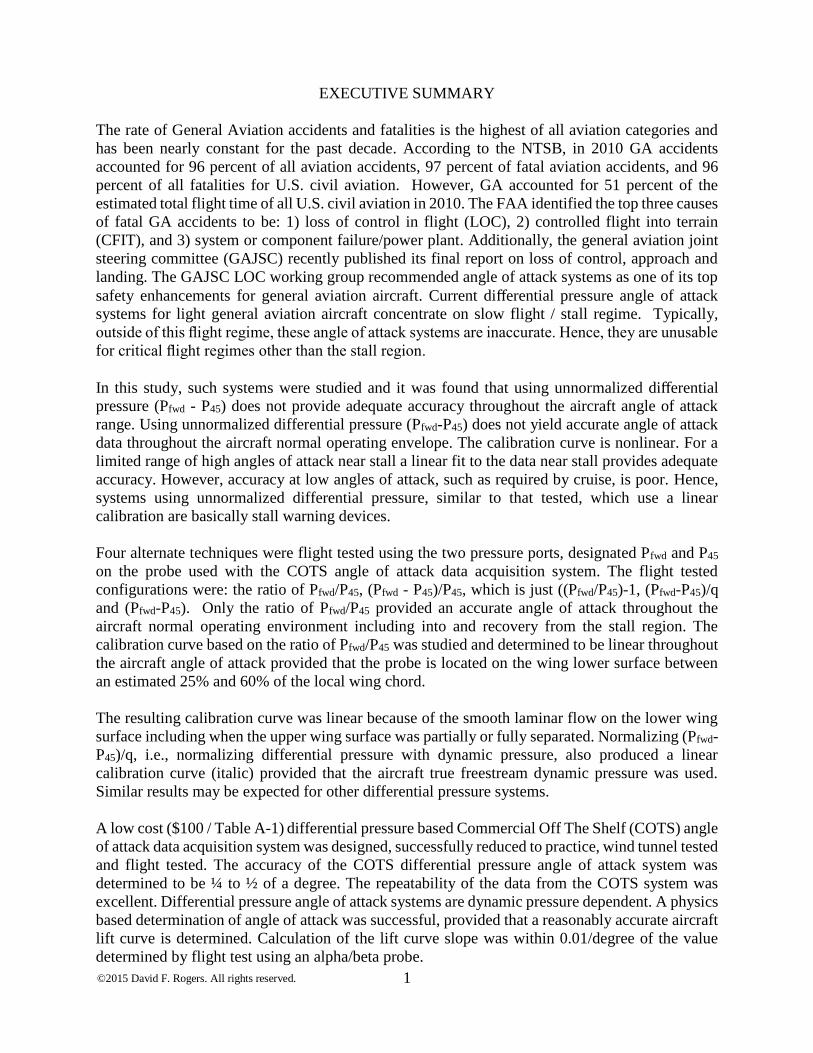
Figure 1. Figure 1 shows curves of the power required to maintain level flight versus true airspeed
for various altitudes on a standard day. Clearly, the power required changes with altitude.
It is well known that, for a piston/propeller aircraft, a line drawn though the origin tangent to the
power required curve yields the speed for maximum lift to drag ratio as illustrated by the
dashed line in Figure 1. The speed for maximum lift to drag ratio is also the speed for maximum
range as well as the speed for best glide. Notice that the single dashed line touches every single
one of the power required curves for the various altitudes. One could say that the power required
curve slides along the line for maximum lift to drag ratio with increasing altitude. Hence, the true
airspeed increases with increasing altitude.
However, the angle between the line for maximum lift to drag ratio remains the same, i.e., there is
only one dashed line for all altitudes. The angle between the dashed line and the abcissa (x-axis)
is directly related to the absolute angle of attack for maximum lift to drag ratio. Thus, the angle of
attack for maximum lift to drag ratio does not depend on density altitude.
*The following is based on a paper by David F. Rogers available at www.nar-associates.com/technical-flying.html
#Angle, Rogers, David F., “Fundamental Angle of Attack”.
©2015 David F. Rogers. All rights reserved.
2
2.1. NONDIMENSIONALIZATION
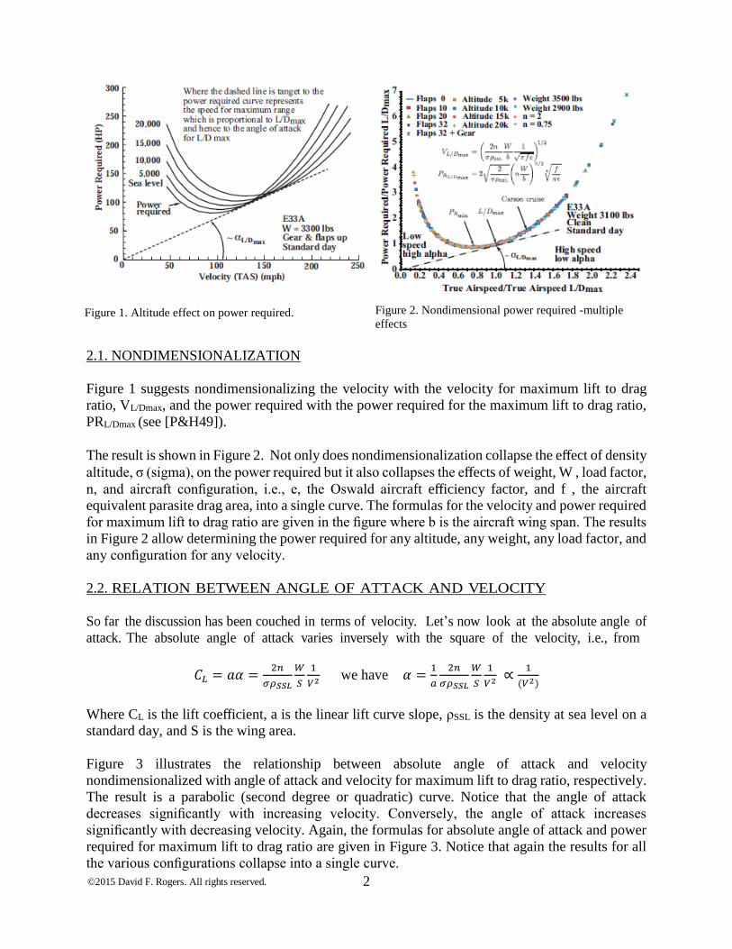
Figure 1 suggests nondimensionalizing the velocity with the velocity for maximum lift to drag
ratio, VL/Dmax, and the power required with the power required for the maximum lift to drag ratio,
PRL/Dmax (see [P&H49]).
The result is shown in Figure 2. Not only does nondimensionalization collapse the effect of density
altitude, σ (sigma), on the power required but it also collapses the effects of weight, W , load factor,
n, and aircraft configuration, i.e., e, the Oswald aircraft efficiency factor, and f , the aircraft
equivalent parasite drag area, into a single curve. The formulas for the velocity and power required
for maximum lift to drag ratio are given in the figure where b is the aircraft wing span. The results
in Figure 2 allow determining the power required for any altitude, any weight, any load factor, and
any configuration for any velocity.
2.2. RELATION BETWEEN ANGLE OF ATTACK AND VELOCITY
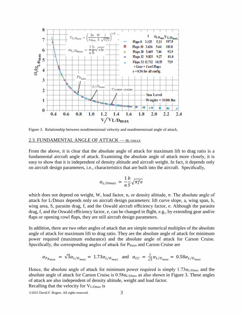
So far the discussion has been couched in terms of velocity. Let’s now look at the absolute angle of
attack. The absolute angle of attack varies inversely with the square of the velocity, i.e., from
𝐶𝐿 = 𝑎𝛼 =2𝑛
𝜎𝜌𝑆𝑆𝐿
𝑊
𝑆
1
𝑉2 we have 𝛼 =1
𝑎
2𝑛
𝜎𝜌𝑆𝑆𝐿
𝑊
𝑆
1
𝑉2 ∝1
(𝑉2)
Where CL is the lift coefficient, a is the linear lift curve slope, ρSSL is the density at sea level on a
standard day, and S is the wing area.
Figure 3 illustrates the relationship between absolute angle of attack and velocity
nondimensionalized with angle of attack and velocity for maximum lift to drag ratio, respectively.
The result is a parabolic (second degree or quadratic) curve. Notice that the angle of attack
decreases significantly with increasing velocity. Conversely, the angle of attack increases
significantly with decreasing velocity. Again, the formulas for absolute angle of attack and power
required for maximum lift to drag ratio are given in Figure 3. Notice that again the results for all
the various configurations collapse into a single curve.
Figure 1. Altitude effect on power required. Figure 2. Nondimensional power required -multiple
effects
©2015 David F. Rogers. All rights reserved.
3
Figure 3. Relationship between nondimensional velocity and nondimensional angle of attack.
2.3. FUNDAMENTAL ANGLE OF ATTACK — αL/DMAX
From the above, it is clear that the absolute angle of attack for maximum lift to drag ratio is a
fundamental aircraft angle of attack. Examining the absolute angle of attack more closely, it is
easy to show that it is independent of density altitude and aircraft weight. In fact, it depends only
on aircraft design parameters, i.e., characteristics that are built into the aircraft. Specifically,
𝛼𝐿 𝐷⁄ 𝑚𝑎𝑥 = 1
𝑎
𝑏
𝑆√𝜋𝑓𝑒
which does not depend on weight, W, load factor, n, or density altitude, σ. The absolute angle of
attack for L/Dmax depends only on aircraft design parameters: lift curve slope, a, wing span, b,
wing area, S, parasite drag, f, and the Oswald aircraft efficiency factor, e. Although the parasite
drag, f, and the Oswald efficiency factor, e, can be changed in flight, e.g., by extending gear and/or
flaps or opening cowl flaps, they are still aircraft design parameters.
In addition, there are two other angles of attack that are simple numerical multiples of the absolute
angle of attack for maximum lift to drag ratio. They are the absolute angle of attack for minimum
power required (maximum endurance) and the absolute angle of attack for Carson Cruise.
Specifically, the corresponding angles of attack for PRmin and Carson Cruise are
𝛼𝑃𝑅𝑚𝑖𝑛 = √3𝛼𝐿 𝐷⁄ 𝑚𝑎𝑥= 1.73𝛼𝐿 𝐷⁄ 𝑚𝑎𝑥
and 𝛼𝐶𝐶 = 1
√3𝛼𝐿 𝐷⁄ 𝑚𝑎𝑥
= 0.58𝛼𝐿 𝐷⁄ 𝑚𝑎𝑥
Hence, the absolute angle of attack for minimum power required is simply 1.73αL/Dmax and the
absolute angle of attack for Carson Cruise is 0.58αL/Dmax as also shown in Figure 3. These angles
of attack are also independent of density altitude, weight and load factor.
Recalling that the velocity for VL/Dmax is
©2015 David F. Rogers. All rights reserved.
4
𝑉𝐿 𝐷⁄ 𝑚𝑎𝑥= (
2𝑛
𝜎𝜌𝑆𝑆𝐿
𝑊
𝑏
1
√𝜋𝑓𝑒)
1 2⁄
the velocities for VPRmin and VCC are also multiples of the VL/Dmax. Specifically,
𝑉𝑃𝑅𝑚𝑖𝑛 =1
√34 𝑉𝐿 𝐷⁄ 𝑚𝑎𝑥
= 0.76𝑉𝐿 𝐷⁄ 𝑚𝑎𝑥 and 𝑉𝐶𝐶 =
1
√34 𝑉𝐿 𝐷⁄ 𝑚𝑎𝑥
= 1.32𝑉𝐿 𝐷⁄ 𝑚𝑎𝑥
However, the velocity (TAS) for VL/Dmax does depend on weight, density altitude and load factor,
as shown by the equations above and in Figure 3. Hence, the velocity for minimum power required
and Carson Cruise also depend on weight, density altitude and load factor.
2.4. POWER REQUIRED AND ANGLE OF ATTACK
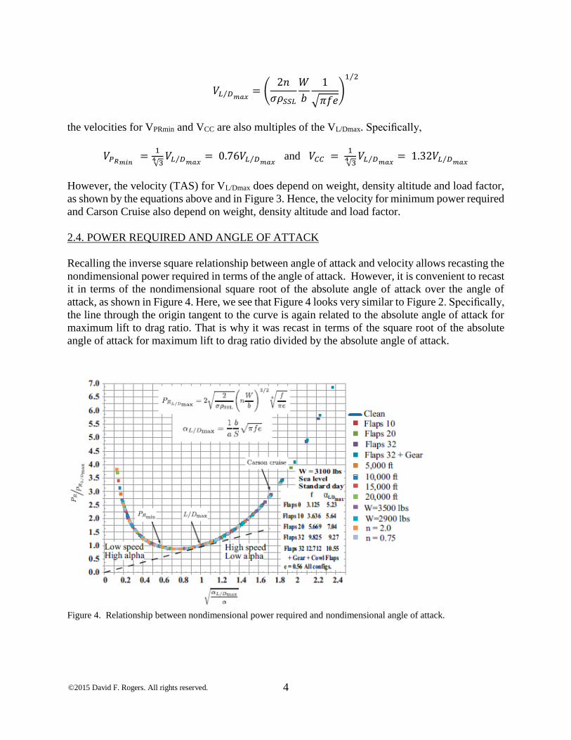
Recalling the inverse square relationship between angle of attack and velocity allows recasting the
nondimensional power required in terms of the angle of attack. However, it is convenient to recast
it in terms of the nondimensional square root of the absolute angle of attack over the angle of
attack, as shown in Figure 4. Here, we see that Figure 4 looks very similar to Figure 2. Specifically,
the line through the origin tangent to the curve is again related to the absolute angle of attack for
maximum lift to drag ratio. That is why it was recast in terms of the square root of the absolute
angle of attack for maximum lift to drag ratio divided by the absolute angle of attack.
Figure 4. Relationship between nondimensional power required and nondimensional angle of attack.
©2015 David F. Rogers. All rights reserved.
5
Figure 5. Probe mounted in the wind tunnel.
2.5. WHY IS FLYING ANGLE OF ATTACK IMPORTANT?
Why is it important to understand that VL/Dmax varies with weight but that αL/Dmax does not? To see
this, look at the speed for L/Dmax (best range speed) for a typical 3300 lb single engine retractable
gear aircraft. With a single pilot and some equipment aboard, that aircraft might typically depart
with full fuel at 2900 lbs. The pilot operating handbook gives the equivalent airspeed in knots
(KEAS) at full gross weight as 105 KEAS. That aircraft might carry 74 gallons of useable fuel.
KEAS for VL/Dmax decreases with decreasing weight as the square root of the weight ratio. For full
fuel at 2900 lbs the equivalent airspeed for VL/Dmax is approximately 98 KEAS. At half fuel it is
approximately 95 KEAS, while with empty tanks it is approximately 90 KEAS. However, the
angle of attack αL/Dmax remains constant. Flying angle of attack might make the mission possible
whether it is to the mission destination or, in an emergency, a glide to an on airport landing rather
than an off airport landing. Furthermore, no calculations are required. Simply fly the angle of
attack. Similar arguments apply to Carson Cruise and minimum power required (see Figure 2).
3. WIND TUNNEL TESTS
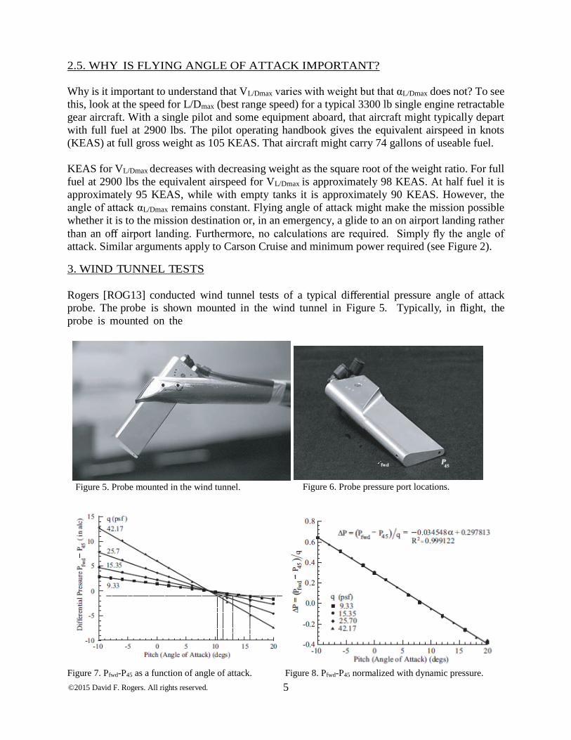
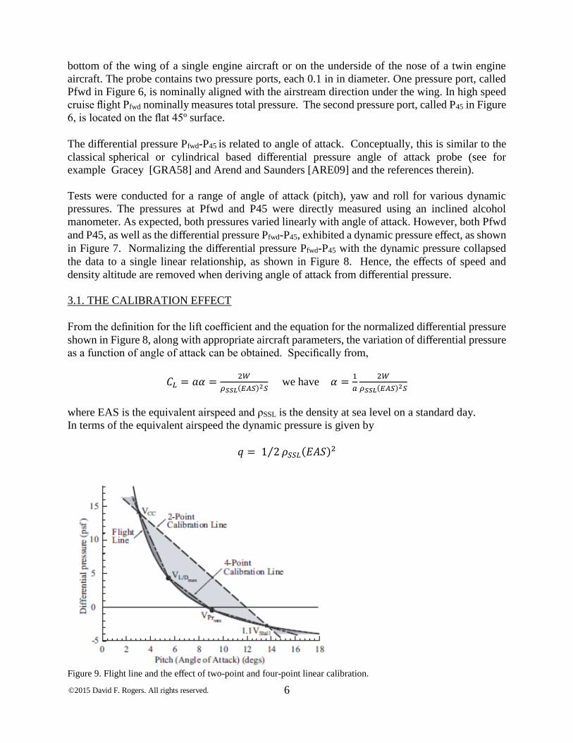
Rogers [ROG13] conducted wind tunnel tests of a typical differential pressure angle of attack
probe. The probe is shown mounted in the wind tunnel in Figure 5. Typically, in flight, the
probe is mounted on the
Figure 6. Probe pressure port locations.
Figure 7. Pfwd-P45 as a function of angle of attack. Figure 8. Pfwd-P45 normalized with dynamic pressure.
©2015 David F. Rogers. All rights reserved.
6
bottom of the wing of a single engine aircraft or on the underside of the nose of a twin engine
aircraft. The probe contains two pressure ports, each 0.1 in in diameter. One pressure port, called
Pfwd in Figure 6, is nominally aligned with the airstream direction under the wing. In high speed
cruise flight Pfwd nominally measures total pressure. The second pressure port, called P45 in Figure
6, is located on the flat 45º surface.
The differential pressure Pfwd-P45 is related to angle of attack. Conceptually, this is similar to the
classical spherical or cylindrical based differential pressure angle of attack probe (see for
example Gracey [GRA58] and Arend and Saunders [ARE09] and the references therein).
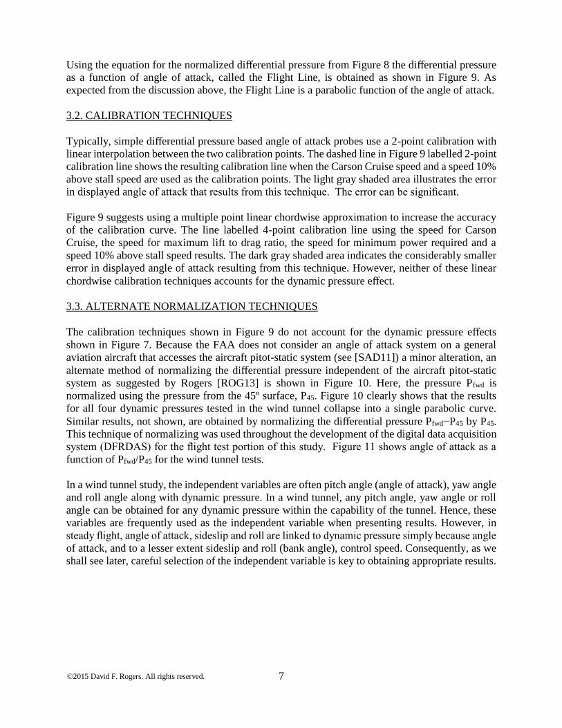
Tests were conducted for a range of angle of attack (pitch), yaw and roll for various dynamic
pressures. The pressures at Pfwd and P45 were directly measured using an inclined alcohol
manometer. As expected, both pressures varied linearly with angle of attack. However, both Pfwd
and P45, as well as the differential pressure Pfwd-P45, exhibited a dynamic pressure effect, as shown
in Figure 7. Normalizing the differential pressure Pfwd-P45 with the dynamic pressure collapsed
the data to a single linear relationship, as shown in Figure 8. Hence, the effects of speed and
density altitude are removed when deriving angle of attack from differential pressure.
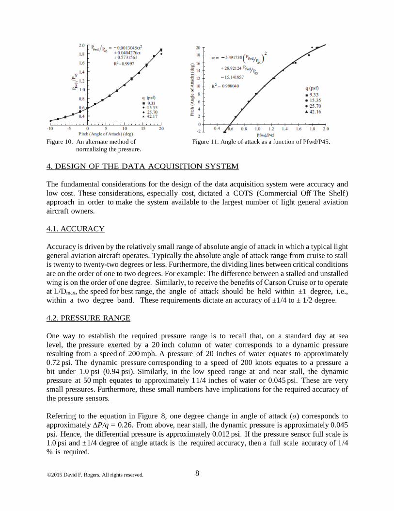
3.1. THE CALIBRATION EFFECT
From the definition for the lift coefficient and the equation for the normalized differential pressure
shown in Figure 8, along with appropriate aircraft parameters, the variation of differential pressure
as a function of angle of attack can be obtained. Specifically from,
𝐶𝐿 = 𝑎𝛼 =2𝑊
𝜌𝑆𝑆𝐿(𝐸𝐴𝑆)2𝑆 we have 𝛼 =
1
𝑎
2𝑊
𝜌𝑆𝑆𝐿(𝐸𝐴𝑆)2𝑆
where EAS is the equivalent airspeed and ρSSL is the density at sea level on a standard day.
In terms of the equivalent airspeed the dynamic pressure is given by
𝑞 = 1 2⁄ 𝜌𝑆𝑆𝐿(𝐸𝐴𝑆)2
Figure 9. Flight line and the effect of two-point and four-point linear calibration.
©2015 David F. Rogers. All rights reserved.
7
Using the equation for the normalized differential pressure from Figure 8 the differential pressure
as a function of angle of attack, called the Flight Line, is obtained as shown in Figure 9. As
expected from the discussion above, the Flight Line is a parabolic function of the angle of attack.
3.2. CALIBRATION TECHNIQUES
Typically, simple differential pressure based angle of attack probes use a 2-point calibration with
linear interpolation between the two calibration points. The dashed line in Figure 9 labelled 2-point
calibration line shows the resulting calibration line when the Carson Cruise speed and a speed 10%
above stall speed are used as the calibration points. The light gray shaded area illustrates the error
in displayed angle of attack that results from this technique. The error can be significant.
Figure 9 suggests using a multiple point linear chordwise approximation to increase the accuracy
of the calibration curve. The line labelled 4-point calibration line using the speed for Carson
Cruise, the speed for maximum lift to drag ratio, the speed for minimum power required and a
speed 10% above stall speed results. The dark gray shaded area indicates the considerably smaller
error in displayed angle of attack resulting from this technique. However, neither of these linear
chordwise calibration techniques accounts for the dynamic pressure effect.
3.3. ALTERNATE NORMALIZATION TECHNIQUES
The calibration techniques shown in Figure 9 do not account for the dynamic pressure effects
shown in Figure 7. Because the FAA does not consider an angle of attack system on a general
aviation aircraft that accesses the aircraft pitot-static system (see [SAD11]) a minor alteration, an
alternate method of normalizing the differential pressure independent of the aircraft pitot-static
system as suggested by Rogers [ROG13] is shown in Figure 10. Here, the pressure Pfwd is
normalized using the pressure from the 45º surface, P45. Figure 10 clearly shows that the results
for all four dynamic pressures tested in the wind tunnel collapse into a single parabolic curve.
Similar results, not shown, are obtained by normalizing the differential pressure Pfwd−P45 by P45.
This technique of normalizing was used throughout the development of the digital data acquisition
system (DFRDAS) for the flight test portion of this study. Figure 11 shows angle of attack as a
function of Pfwd/P45 for the wind tunnel tests.
In a wind tunnel study, the independent variables are often pitch angle (angle of attack), yaw angle
and roll angle along with dynamic pressure. In a wind tunnel, any pitch angle, yaw angle or roll
angle can be obtained for any dynamic pressure within the capability of the tunnel. Hence, these
variables are frequently used as the independent variable when presenting results. However, in
steady flight, angle of attack, sideslip and roll are linked to dynamic pressure simply because angle
of attack, and to a lesser extent sideslip and roll (bank angle), control speed. Consequently, as we
shall see later, careful selection of the independent variable is key to obtaining appropriate results.
©2015 David F. Rogers. All rights reserved.
8
Figure 10. An alternate method of Figure 11. Angle of attack as a function of Pfwd/P45.
normalizing the pressure.
4. DESIGN OF THE DATA ACQUISITION SYSTEM
The fundamental considerations for the design of the data acquisition system were accuracy and
low cost. These considerations, especially cost, dictated a COTS (Commercial Off The Shelf)
approach in order to make the system available to the largest number of light general aviation
aircraft owners.
4.1. ACCURACY
Accuracy is driven by the relatively small range of absolute angle of attack in which a typical light
general aviation aircraft operates. Typically the absolute angle of attack range from cruise to stall
is twenty to twenty-two degrees or less. Furthermore, the dividing lines between critical conditions
are on the order of one to two degrees. For example: The difference between a stalled and unstalled
wing is on the order of one degree. Similarly, to receive the benefits of Carson Cruise or to operate
at L/Dmax, the speed for best range, the angle of attack should be held within ±1 degree, i.e.,
within a two degree band. These requirements dictate an accuracy of ±1/4 to ± 1/2 degree.
4.2. PRESSURE RANGE
One way to establish the required pressure range is to recall that, on a standard day at sea
level, the pressure exerted by a 20 inch column of water corresponds to a dynamic pressure
resulting from a speed of 200 mph. A pressure of 20 inches of water equates to approximately
0.72 psi. The dynamic pressure corresponding to a speed of 200 knots equates to a pressure a
bit under 1.0 psi (0.94 psi). Similarly, in the low speed range at and near stall, the dynamic
pressure at 50 mph equates to approximately 11/4 inches of water or 0.045 psi. These are very
small pressures. Furthermore, these small numbers have implications for the required accuracy of
the pressure sensors.
Referring to the equation in Figure 8, one degree change in angle of attack (α) corresponds to
approximately ∆P/q = 0.26. From above, near stall, the dynamic pressure is approximately 0.045
psi. Hence, the differential pressure is approximately 0.012 psi. If the pressure sensor full scale is
1.0 psi and ±1/4 degree of angle attack is the required accuracy, then a full scale accuracy of 1/4
% is required.

©2015 David F. Rogers. All rights reserved.
9
4.3. REFERENCE PRESSURE
All pressure measurements are differential. A so called absolute pressure gauge is simply a
differential pressure gauge with a built in reference pressure. An example is the Bourdon tube
in an altimeter. The original wind tunnel tests used the local atmospheric pressure for the
reference pressure. The question becomes: What to use as a reference pressure for the digital data
acquisition system while in flight? This becomes particularly important considering the range of
‘local’ atmospheric pressure and temperature as the aircraft climbs and descends.
4.4. PRESSURE SENSORS
The Measurement Specialties MS4525DO differential pressure sensor was chosen because of
commercial availability and l o w cost ($21 / Table A-1). Specifically the MS4525DO-DS-5-
A-I-001-D-P was used [MSa]. This unit, shown in Figure 12, is a small, ceramic based, PC
board mounted low power pressure transducer with a 14 bit digital temperature compensated (11
bit) output. Full scale output is 1.0 psi with an accuracy of ± 1/4 % of full scale. The 1/8 inch
barbed pressure ports mate securely with 3/32 ID tubing. The sensor is designed to operate at either
3.3 or 5.0 VDC. The sensor is compatible with either the I2C or SPI bus. Multiple I2C addresses
are specified although only one I2C address was available for the sensors used for the data
acquisition system.
Because of concerns with the reference pressure, an additional sensor was included in the data
acquisition
System design. The Bosch BMP085 [BM085] was chosen, again, because of commercial
availability and cost. The BMP085, shown in Figure 13, and its replacement the BMP180, are
high-precision, ultra-low power barometric pressure sensors. Their accuracy is of the order of 2.5
hPa with low noise level down to 0.03 hPa, which is equivalent to an altitude change of
approximately 8 inches. Conversion to local atmospheric pressure is straightforward. Digital
temperature measurement is also available from the sensor. The BMP085 is about the size of a
quarter. The BMP085, and BMP180, are also compatible with the I2C bus.
Figure 12. MS4525 differential pressure sensor. Figure 13. Bosch BMP085 altitude/pressure absolute pressure
sensor.
©2015 David F. Rogers. All rights reserved.
10
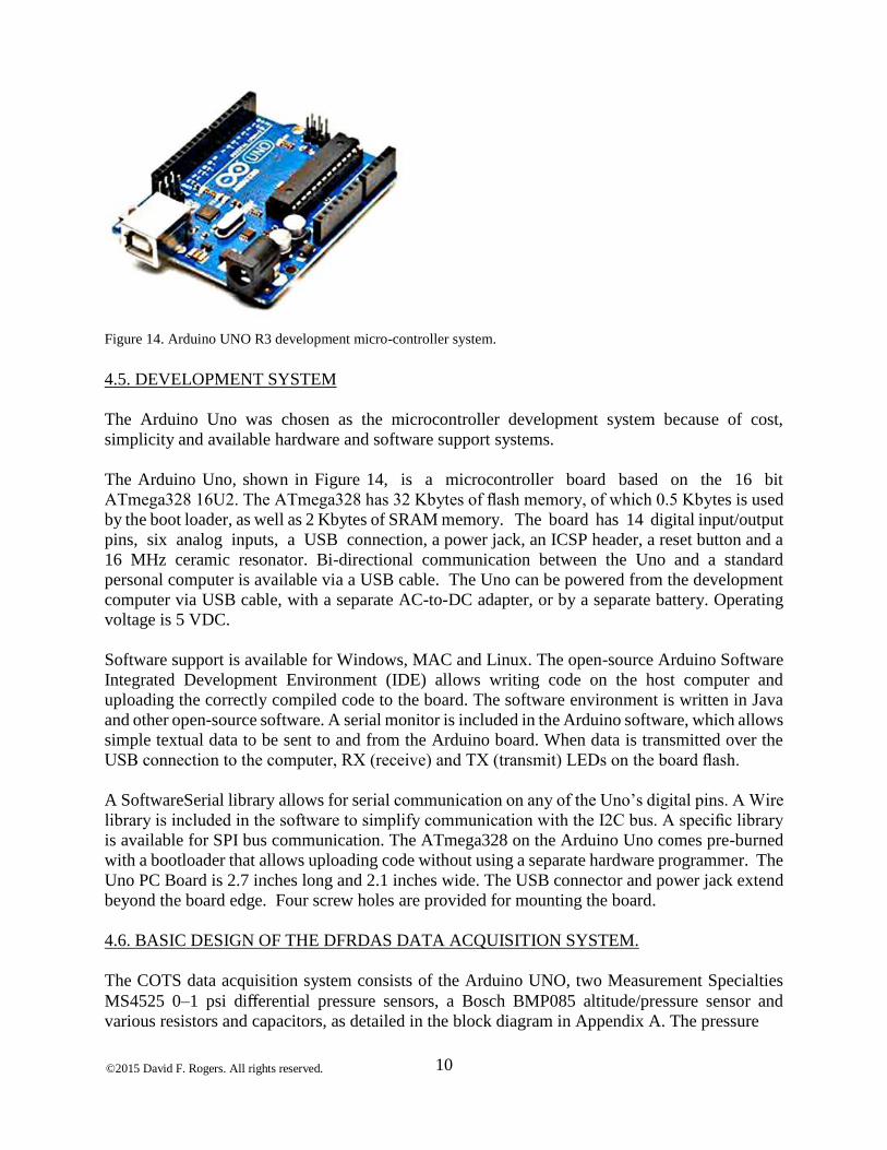
Figure 14. Arduino UNO R3 development micro-controller system.
4.5. DEVELOPMENT SYSTEM
The Arduino Uno was chosen as the microcontroller development system because of cost,
simplicity and available hardware and software support systems.
The Arduino Uno, shown in Figure 14, is a microcontroller board based on the 16 bit
ATmega328 16U2. The ATmega328 has 32 Kbytes of flash memory, of which 0.5 Kbytes is used
by the boot loader, as well as 2 Kbytes of SRAM memory. The board has 14 digital input/output
pins, six analog inputs, a USB connection, a power jack, an ICSP header, a reset button and a
16 MHz ceramic resonator. Bi-directional communication between the Uno and a standard
personal computer is available via a USB cable. The Uno can be powered from the development
computer via USB cable, with a separate AC-to-DC adapter, or by a separate battery. Operating
voltage is 5 VDC.
Software support is available for Windows, MAC and Linux. The open-source Arduino Software
Integrated Development Environment (IDE) allows writing code on the host computer and
uploading the correctly compiled code to the board. The software environment is written in Java
and other open-source software. A serial monitor is included in the Arduino software, which allows
simple textual data to be sent to and from the Arduino board. When data is transmitted over the
USB connection to the computer, RX (receive) and TX (transmit) LEDs on the board flash.
A SoftwareSerial library allows for serial communication on any of the Uno’s digital pins. A Wire
library is included in the software to simplify communication with the I2C bus. A specific library
is available for SPI bus communication. The ATmega328 on the Arduino Uno comes pre-burned
with a bootloader that allows uploading code without using a separate hardware programmer. The
Uno PC Board is 2.7 inches long and 2.1 inches wide. The USB connector and power jack extend
beyond the board edge. Four screw holes are provided for mounting the board.
4.6. BASIC DESIGN OF THE DFRDAS DATA ACQUISITION SYSTEM.
The COTS data acquisition system consists of the Arduino UNO, two Measurement Specialties
MS4525 0–1 psi differential pressure sensors, a Bosch BMP085 altitude/pressure sensor and
various resistors and capacitors, as detailed in the block diagram in Appendix A. The pressure
©2015 David F. Rogers. All rights reserved.
11
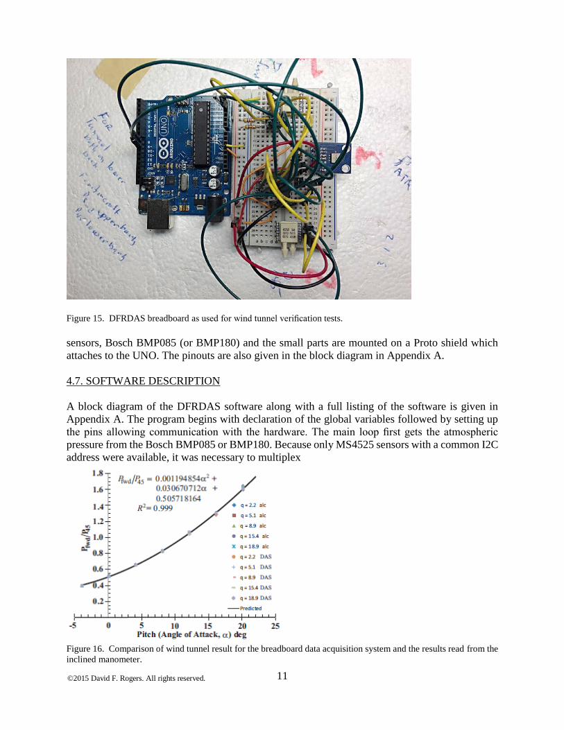
Figure 15. DFRDAS breadboard as used for wind tunnel verification tests.
sensors, Bosch BMP085 (or BMP180) and the small parts are mounted on a Proto shield which
attaches to the UNO. The pinouts are also given in the block diagram in Appendix A.
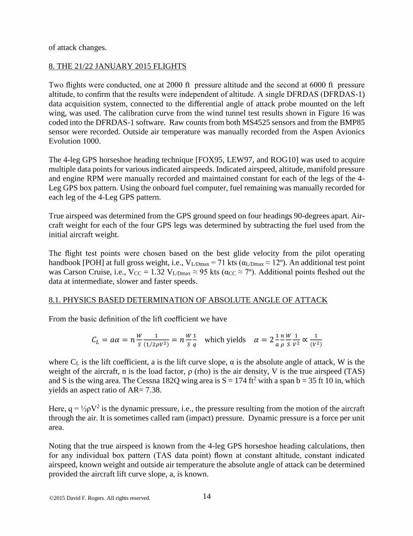
4.7. SOFTWARE DESCRIPTION
A block diagram of the DFRDAS software along with a full listing of the software is given in
Appendix A. The program begins with declaration of the global variables followed by setting up
the pins allowing communication with the hardware. The main loop first gets the atmospheric
pressure from the Bosch BMP085 or BMP180. Because only MS4525 sensors with a common I2C
address were available, it was necessary to multiplex
Figure 16. Comparison of wind tunnel result for the breadboard data acquisition system and the results read from the
inclined manometer.

©2015 David F. Rogers. All rights reserved.
12
accessing the two MS4525 pressure sensors for Pfwd and P45. The Pfwd and P45 pressure values are
acquired as raw counts in the range of 0 to 16383. These values are corrected by subtracting the
‘noload’ values corresponding to zero differential pressure. The ratio Pfwd/P45 is then calculated
using the ‘noload’ corrected Pfwd and P45 values. The angle of attack, α, is then determined from
the calibration equation. Finally, the result is either printed or displayed as required.
4.8. WIND TUNNEL TESTING OF THE DFRDAS BREADBOARD
To insure that the breadboard data acquisition system, shown in Figure 15, worked correctly and
provided appropriate accuracy, a wind tunnel test was conducted. The angle of attack probe was
set up in the wind tunnel exactly as reported by Rogers [ROG13] with the exception that the
Pfwd and P45 pressure lines were T’d to the breadboard data acquisition system. Fifty samples
were simultaneously collected by the breadboard data acquisition system while the inclined
alcohol manometer was manually read. The angle of attack probe was pitched from −6◦ to
18◦ in four degree increments for dynamic pressures of 2.2, 5.1, 8.9, 15.4 and 19.9 inches of
alcohol. The samples acquired by the breadboard data acquisition system were corrected for the
noload condition and then were averaged to yield Pfwd/P45. The local barometric pressure was used
as the reference pressure for both the inclined alcohol manometer and for the MS4525 pressure
sensors in the breadboard data acquisition system. The results for both the alcohol and breadboard
data acquisition system are shown in Figure 16. The accuracy of the pitch attitude of the wind
tunnel balance is 0.1◦. Clearly, the breadboard data acquisition system is of equal or better accuracy
under the flow conditions present in the wind tunnel.
Furthermore, clearly in the static environment of the wind tunnel room, using the local room
atmospheric pressure as the reference pressure for the data acquisition system was satisfactory.
However, considering the large variation of atmospheric pressure with altitude, the question
remained: Would using the local atmospheric pressure as the reference pressure work for the
MS4525 sensors?
4.9. NOLOAD ALTITUDE TEST
The breadboard data acquisition system was tested for variation in the noload (bias) values at
altitudes from near sea level (15 ft) to 6000 ft in 1000 ft increments. While in steady level flight, a
sample of 500 noload values was taken for both the Pfwd and P45 sensors. The standard deviation
for the 500 noload values was on the order of 10 counts out of 16383 possible counts. The
maximum observed change in the noload value was 22 counts. For Pfwd the noload count decreased
slightly with increasing altitude while for P45 the noload count increased slightly for increasing
altitude. These changes are small and are attributed to individual sensor calibration by the
manufacturer and possibly to temperatures changes with altitude. The maximum observed change
represents approximately 0.1% of full scale for the sensor.
5. ROAD TESTS
The wind tunnel used for the angle of attack probe tests is a straight through design (Eiffel) tunnel
which uses the surrounding room as the plenum; the test section is sealed. Hence, both the Pfwd
and P45 pressures are below atmospheric pressure. Consequently, the lower (No. 1) barb on the
MS4525 is used to measure pressure. The upper barb is left open to the local atmospheric pressure.

©2015 David F. Rogers. All rights reserved.
13
However, in flight, Pfwd, at typical flight attitudes, is nominally the total pressure, i.e., the dynamic
pressure plus the static pressure. In flight, the static pressure is nominally the local atmospheric
pressure. Thus, Pfwd is normally greater than the local atmospheric pressure, and hence positive,
and the lower (No. 1) barb on the MS4525 is used to measure Pfwd and the upper (No. 2) barb is
used for the reference pressure.
If the local atmospheric pressure is used as the reference pressure for P45, the result is not as clear.
If the pressure at P45 is less than the local atmospheric pressure, then, when corrected for the noload
value, a negative value of P45 results. If that is the case, then solving the quadratic calibration
equation given in Figure 16 is problematic, especially at the low dynamic pressures associated
with speeds near stall.
Consequently, a rig was developed which, mounted on a truck, allowed testing the breadboard data
acquisition system at low speeds. The rig consisted of a PVC pipe attached to a pair of roof racks
on the truck cab. The pipe projected forward approximately over the truck hood. The probe was
mounted to the forward end of the PVC pipe.
Road tests were conducted at 25 and 60 mph for all four possible barb connections. The results
suggested that both Pfwd and P45 are positive for the anticipated probe pitch angles. Hence, both
Pfwd and P45 pressure sensors were connected to the lower No. 1 position, as shown in the MS4525
data sheet [MS45] for the flight tests. In addition, the turbulence on the highway was clearly shown
in the acquired data which suggested that the DFRDAS was both fast enough and sensitive enough.
6. PROOF OF CONCEPT FLIGHT TEST
An initial proof of concept flight test was conducted at Bay Bridge Airport (W29) on 21 & 22
January 2015. The purpose of the flight tests was to confirm that:
1. the DFRDAS mechanically and electrically worked in flight;
2. the DFRDAS had an adequate data acquisition sample rate in flight;
3. the local atmospheric pressure as the reference pressure when determining Pfwd/P45
correctly normalized the pressures;
4. the Pfwd /P45 curves for different altitudes collapsed into a single curve.
7. THE AIRCRAFT
The aircraft used was a Cessna 182Q. The aircraft was not equipped with an angle of attack/angle
of sideslip (α/β) boom for these flights. A standard general aviation differential pressure angle of
attack probe, as used in the wind tunnel tests, was mounted on the left wing in an inspection port
centered approximately 13 in outboard of the wing strut attachment. The center of the probe
inspection port was approximately four inches aft of the leading edge which placed Pfwd
approximately at the leading edge.
Mounting the differential pressure angle of attack probe at the leading edge is outside of the
manufacturer’s recommendation. Mounted this far forward the probe is in the upwash field ahead
of the wing. It may also be in the critical area where the surface pressure on the wing changes from
positive to negative with respect to the local atmospheric pressure [GAR34] as the aircraft angle
©2015 David F. Rogers. All rights reserved.
14
of attack changes.
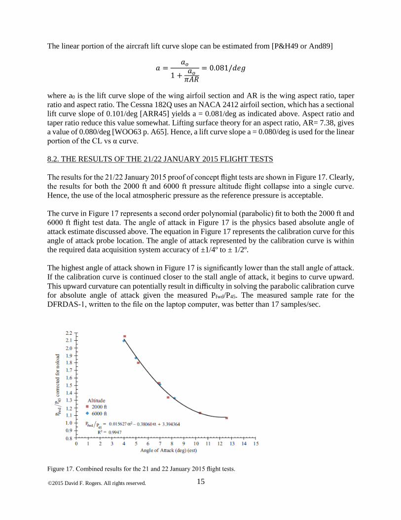
8. THE 21/22 JANUARY 2015 FLIGHTS
Two flights were conducted, one at 2000 ft pressure altitude and the second at 6000 ft pressure
altitude, to confirm that the results were independent of altitude. A single DFRDAS (DFRDAS-1)
data acquisition system, connected to the differential angle of attack probe mounted on the left
wing, was used. The calibration curve from the wind tunnel test results shown in Figure 16 was
coded into the DFRDAS-1 software. Raw counts from both MS4525 sensors and from the BMP85
sensor were recorded. Outside air temperature was manually recorded from the Aspen Avionics
Evolution 1000.
The 4-leg GPS horseshoe heading technique [FOX95, LEW97, and ROG10] was used to acquire
multiple data points for various indicated airspeeds. Indicated airspeed, altitude, manifold pressure
and engine RPM were manually recorded and maintained constant for each of the legs of the 4-
Leg GPS box pattern. Using the onboard fuel computer, fuel remaining was manually recorded for
each leg of the 4-Leg GPS pattern.
True airspeed was determined from the GPS ground speed on four headings 90-degrees apart. Air-
craft weight for each of the four GPS legs was determined by subtracting the fuel used from the
initial aircraft weight.
The flight test points were chosen based on the best glide velocity from the pilot operating
handbook [POH] at full gross weight, i.e., VL/Dmax = 71 kts (αL/Dmax ≈ 12º). An additional test point
was Carson Cruise, i.e., VCC = 1.32 VL/Dmax ≈ 95 kts (αCC ≈ 7º). Additional points fleshed out the
data at intermediate, slower and faster speeds.
8.1. PHYSICS BASED DETERMINATION OF ABSOLUTE ANGLE OF ATTACK
From the basic definition of the lift coefficient we have
𝐶𝐿 = 𝑎𝛼 = 𝑛𝑊
𝑆
1
(1 2⁄ 𝜌𝑉2)= 𝑛
𝑊
𝑆
1
𝑞 which yields 𝛼 = 2
1
𝑎
𝑛
𝜌
𝑊
𝑆
1
𝑉2 ∝1
(𝑉2)
where CL is the lift coefficient, a is the lift curve slope, α is the absolute angle of attack, W is the
weight of the aircraft, n is the load factor, ρ (rho) is the air density, V is the true airspeed (TAS)
and S is the wing area. The Cessna 182Q wing area is S = 174 ft2 with a span b = 35 ft 10 in, which
yields an aspect ratio of AR= 7.38.
Here, q = ½ρV2 is the dynamic pressure, i.e., the pressure resulting from the motion of the aircraft
through the air. It is sometimes called ram (impact) pressure. Dynamic pressure is a force per unit
area.
Noting that the true airspeed is known from the 4-leg GPS horseshoe heading calculations, then
for any individual box pattern (TAS data point) flown at constant altitude, constant indicated
airspeed, known weight and outside air temperature the absolute angle of attack can be determined
provided the aircraft lift curve slope, a, is known.
©2015 David F. Rogers. All rights reserved.
15
The linear portion of the aircraft lift curve slope can be estimated from [P&H49 or And89]
𝑎 =𝑎𝑜
1 +𝑎𝑜
𝜋𝐴𝑅
= 0.081/𝑑𝑒𝑔
where a0 is the lift curve slope of the wing airfoil section and AR is the wing aspect ratio, taper
ratio and aspect ratio. The Cessna 182Q uses an NACA 2412 airfoil section, which has a sectional
lift curve slope of 0.101/deg [ARR45] yields a = 0.081/deg as indicated above. Aspect ratio and
taper ratio reduce this value somewhat. Lifting surface theory for an aspect ratio, AR= 7.38, gives
a value of 0.080/deg [WOO63 p. A65]. Hence, a lift curve slope a = 0.080/deg is used for the linear
portion of the CL vs α curve.
8.2. THE RESULTS OF THE 21/22 JANUARY 2015 FLIGHT TESTS
The results for the 21/22 January 2015 proof of concept flight tests are shown in Figure 17. Clearly,
the results for both the 2000 ft and 6000 ft pressure altitude flight collapse into a single curve.
Hence, the use of the local atmospheric pressure as the reference pressure is acceptable.
The curve in Figure 17 represents a second order polynomial (parabolic) fit to both the 2000 ft and
6000 ft flight test data. The angle of attack in Figure 17 is the physics based absolute angle of
attack estimate discussed above. The equation in Figure 17 represents the calibration curve for this
angle of attack probe location. The angle of attack represented by the calibration curve is within
the required data acquisition system accuracy of ±1/4º to ± 1/2º.
The highest angle of attack shown in Figure 17 is significantly lower than the stall angle of attack.
If the calibration curve is continued closer to the stall angle of attack, it begins to curve upward.
This upward curvature can potentially result in difficulty in solving the parabolic calibration curve
for absolute angle of attack given the measured Pfwd/P45. The measured sample rate for the
DFRDAS-1, written to the file on the laptop computer, was better than 17 samples/sec.
Figure 17. Combined results for the 21 and 22 January 2015 flight tests.
©2015 David F. Rogers. All rights reserved.
16
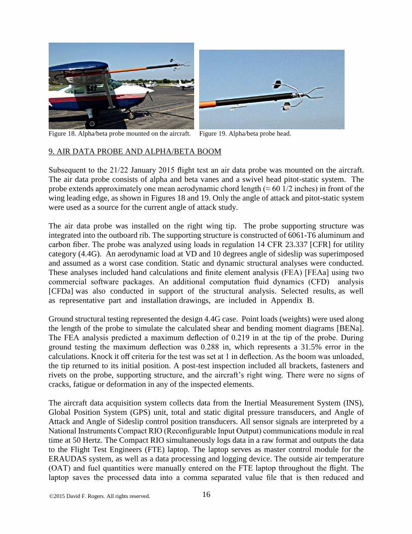
Figure 18. Alpha/beta probe mounted on the aircraft. Figure 19. Alpha/beta probe head.
9. AIR DATA PROBE AND ALPHA/BETA BOOM
Subsequent to the 21/22 January 2015 flight test an air data probe was mounted on the aircraft.
The air data probe consists of alpha and beta vanes and a swivel head pitot-static system. The
probe extends approximately one mean aerodynamic chord length (≈ 60 1/2 inches) in front of the
wing leading edge, as shown in Figures 18 and 19. Only the angle of attack and pitot-static system
were used as a source for the current angle of attack study.
The air data probe was installed on the right wing tip. The probe supporting structure was
integrated into the outboard rib. The supporting structure is constructed of 6061-T6 aluminum and
carbon fiber. The probe was analyzed using loads in regulation 14 CFR 23.337 [CFR] for utility
category (4.4G). An aerodynamic load at VD and 10 degrees angle of sideslip was superimposed
and assumed as a worst case condition. Static and dynamic structural analyses were conducted.
These analyses included hand calculations and finite element analysis (FEA) [FEAa] using two
commercial software packages. An additional computation fluid dynamics (CFD) analysis
[CFDa] was also conducted in support of the structural analysis. Selected results, as well
as representative part and installation drawings, are included in Appendix B.
Ground structural testing represented the design 4.4G case. Point loads (weights) were used along
the length of the probe to simulate the calculated shear and bending moment diagrams [BENa].
The FEA analysis predicted a maximum deflection of 0.219 in at the tip of the probe. During
ground testing the maximum deflection was 0.288 in, which represents a 31.5% error in the
calculations. Knock it off criteria for the test was set at 1 in deflection. As the boom was unloaded,
the tip returned to its initial position. A post-test inspection included all brackets, fasteners and
rivets on the probe, supporting structure, and the aircraft’s right wing. There were no signs of
cracks, fatigue or deformation in any of the inspected elements.
The aircraft data acquisition system collects data from the Inertial Measurement System (INS),
Global Position System (GPS) unit, total and static digital pressure transducers, and Angle of
Attack and Angle of Sideslip control position transducers. All sensor signals are interpreted by a
National Instruments Compact RIO (Reconfigurable Input Output) communications module in real
time at 50 Hertz. The Compact RIO simultaneously logs data in a raw format and outputs the data
to the Flight Test Engineers (FTE) laptop. The laptop serves as master control module for the
ERAUDAS system, as well as a data processing and logging device. The outside air temperature
(OAT) and fuel quantities were manually entered on the FTE laptop throughout the flight. The
laptop saves the processed data into a comma separated value file that is then reduced and
©2015 David F. Rogers. All rights reserved.
17
interpreted post-flight.
Ground calibrations for the total and static digital pressure transducers and angle of attack and
angle of sideslip control position transducers were performed prior to first flight. All ground
calibrations utilized the data acquisition system and were performed “end to end”. The angle of
attack measured by the alpha/beta probe was calibrated with respect to the fuselage reference line.
Details of the ground calibration setup and results are included in Appendix B.
Prior to first flight a safety review board was convened. Configuration control requests, hazard and
risk assessments, and flight test cards were reviewed and approved. A safety finding and flight
permit were issued. Post first flight a second safety review board was convened. The aircraft was
cleared for research flights, an updated safety finding and a flight permit were issued. Details of
the safety review board process are included in Appendix F.
Prior to all research data flights several in-flight calibrations were required for the air data probe.
The probe pitot-static system was calibrated using a GPS 4-Leg maneuver. The probe angle of
attack vane was calibrated using steady trim shots during the GPS 4-Leg maneuver. Details of in-
flight calibrations, theory, practical considerations, and results are included in Appendix B.
10. THE RESULTS OF THE 22 APRIL 2015 FLIGHT TEST
A single test flight was conducted at Daytona Beach (KDAB) on 22 April 2015. Two separate
DFRDAS systems were installed on the flight test aircraft. The left wing Alpha System probe
location and orientation was not changed from the 21/22 January 2015 flight tests. The calibration
curve from Figure 17 was implemented in the left wing data acquisition system (DFRDAS-1)
software. Given Pfwd/P45 from the data acquisition system the quadratic equation in Figure 17 was
solved for the angle of attack. Code was included in the DFRDAS-1 software to check for a
negative radical.
Prior to the 22 April 2015 flight test a second DFRDAS (DFRDAS-2) was built and installed on
the right wing of the flight test aircraft. The second DFRDAS hardware was identical to that of the
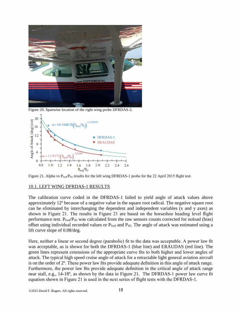
first DFRDAS (DFRDAS-1). The center of the inspection port for the DFRDAS-2 was located at
38.9% of the local chord at the spanwise position shown in Figure 20. The basic software installed
on the DFRDAS-2 was the same as previously installed on the DFRDAS-1 with the exception of
the calibration curve. The wind tunnel calibration curve was implemented in the DFRDAS-2
software.
A seven point horseshoe heading level flight performance test was conducted at a pressure altitude
of 6000 ft. Again, data points were taken at speeds corresponding the VL/Dmax, VCC, VPRmin points
and at maximum available power (117 KIAS).**
Two standard FAA idle power stalls (1 KIAS per second deceleration) were also conducted at an
approximate weight of 2835 lbs. The indicated stall airspeed was 51/52 KIAS.
**The flight test aircraft is not equipped with wheel pants.
©2015 David F. Rogers. All rights reserved.
18
Figure 20. Spanwise location of the right wing probe DFRDAS-2.
Figure 21. Alpha vs Pfwd/P45 results for the left wing DFRDAS-1 probe for the 22 April 2015 flight test.
10.1. LEFT WING DFRDAS-1 RESULTS
The calibration curve coded in the DFRDAS-1 failed to yield angle of attack values above
approximately 12º because of a negative value in the square root radical. The negative square root
can be eliminated by interchanging the dependent and independent variables (x and y axes) as
shown in Figure 21. The results in Figure 21 are based on the horseshoe heading level flight
performance test. Pfwd/P45 was calculated from the raw sensors counts corrected for noload (bias)
offset using individual recorded values or Pfwd and P45. The angle of attack was estimated using a
lift curve slope of 0.08/deg.
Here, neither a linear or second degree (parabolic) fit to the data was acceptable. A power law fit
was acceptable, as is shown for both the DFRDAS-1 (blue line) and ERAUDAS (red line). The
green lines represent extensions of the appropriate curve fits to both higher and lower angles of
attack. The typical high speed cruise angle of attack for a retractable light general aviation aircraft
is on the order of 2º. These power law fits provide adequate definition in this angle of attack range.
Furthermore, the power law fits provide adequate definition in the critical angle of attack range
near stall, e.g., 14-18º, as shown by the data in Figure 21. The DFRDAS-1 power law curve fit
equation shown in Figure 21 is used in the next series of flight tests with the DFRDAS-1.
©2015 David F. Rogers. All rights reserved.
19
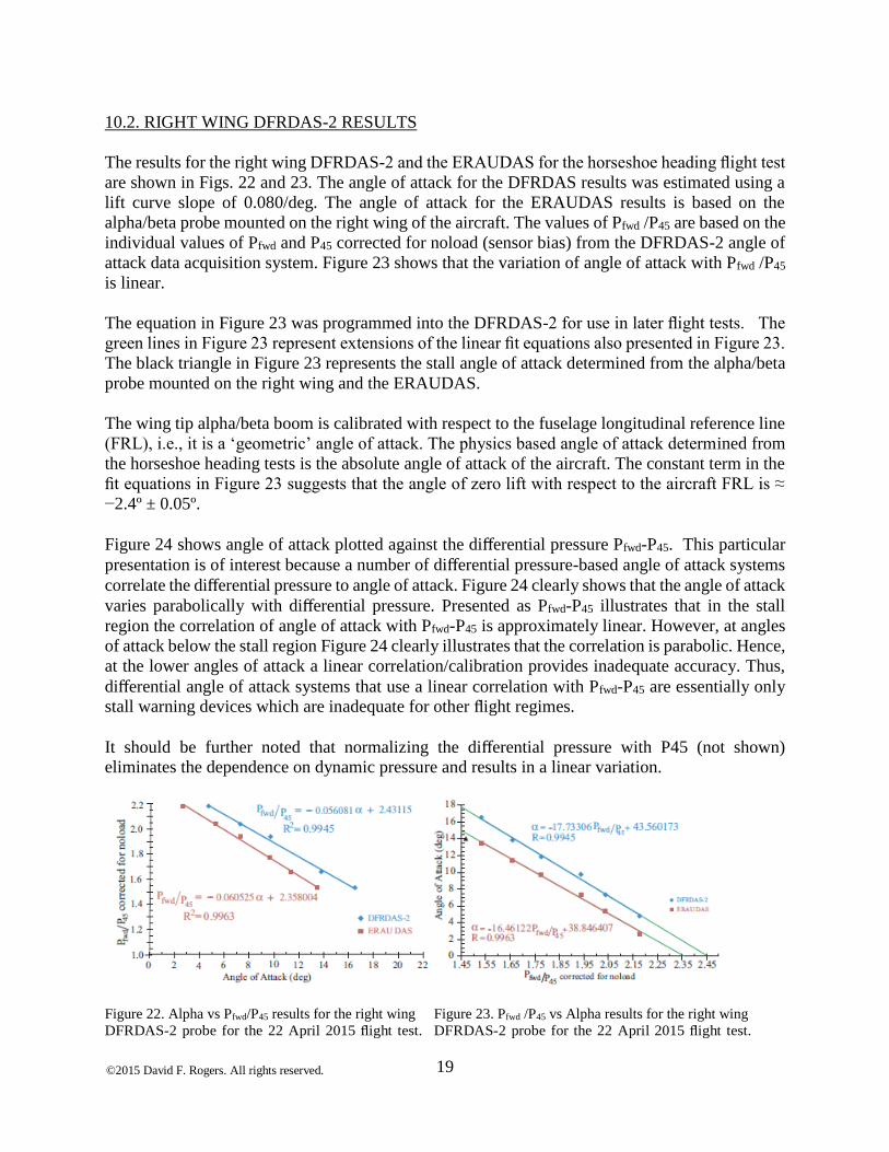
10.2. RIGHT WING DFRDAS-2 RESULTS
The results for the right wing DFRDAS-2 and the ERAUDAS for the horseshoe heading flight test
are shown in Figs. 22 and 23. The angle of attack for the DFRDAS results was estimated using a
lift curve slope of 0.080/deg. The angle of attack for the ERAUDAS results is based on the
alpha/beta probe mounted on the right wing of the aircraft. The values of Pfwd /P45 are based on the
individual values of Pfwd and P45 corrected for noload (sensor bias) from the DFRDAS-2 angle of
attack data acquisition system. Figure 23 shows that the variation of angle of attack with Pfwd /P45
is linear.
The equation in Figure 23 was programmed into the DFRDAS-2 for use in later flight tests. The
green lines in Figure 23 represent extensions of the linear fit equations also presented in Figure 23.
The black triangle in Figure 23 represents the stall angle of attack determined from the alpha/beta
probe mounted on the right wing and the ERAUDAS.
The wing tip alpha/beta boom is calibrated with respect to the fuselage longitudinal reference line
(FRL), i.e., it is a ‘geometric’ angle of attack. The physics based angle of attack determined from
the horseshoe heading tests is the absolute angle of attack of the aircraft. The constant term in the
fit equations in Figure 23 suggests that the angle of zero lift with respect to the aircraft FRL is ≈
−2.4º ± 0.05º.
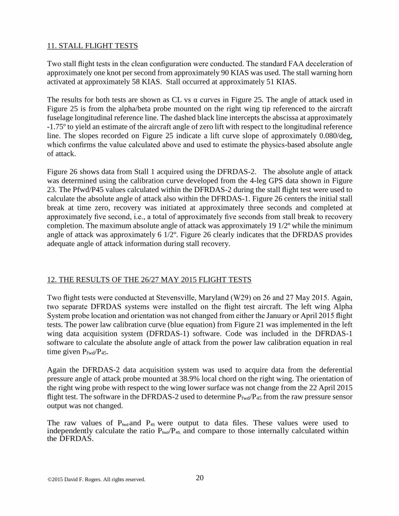
Figure 24 shows angle of attack plotted against the differential pressure Pfwd-P45. This particular
presentation is of interest because a number of differential pressure-based angle of attack systems
correlate the differential pressure to angle of attack. Figure 24 clearly shows that the angle of attack
varies parabolically with differential pressure. Presented as Pfwd-P45 illustrates that in the stall
region the correlation of angle of attack with Pfwd-P45 is approximately linear. However, at angles
of attack below the stall region Figure 24 clearly illustrates that the correlation is parabolic. Hence,
at the lower angles of attack a linear correlation/calibration provides inadequate accuracy. Thus,
differential angle of attack systems that use a linear correlation with Pfwd-P45 are essentially only
stall warning devices which are inadequate for other flight regimes.
It should be further noted that normalizing the differential pressure with P45 (not shown)
eliminates the dependence on dynamic pressure and results in a linear variation.
Figure 22. Alpha vs Pfwd/P45 results for the right wing Figure 23. Pfwd /P45 vs Alpha results for the right wing
DFRDAS-2 probe for the 22 April 2015 flight test. DFRDAS-2 probe for the 22 April 2015 flight test.
©2015 David F. Rogers. All rights reserved.
20
11. STALL FLIGHT TESTS
Two stall flight tests in the clean configuration were conducted. The standard FAA deceleration of
approximately one knot per second from approximately 90 KIAS was used. The stall warning horn
activated at approximately 58 KIAS. Stall occurred at approximately 51 KIAS.
The results for both tests are shown as CL vs α curves in Figure 25. The angle of attack used in
Figure 25 is from the alpha/beta probe mounted on the right wing tip referenced to the aircraft
fuselage longitudinal reference line. The dashed black line intercepts the abscissa at approximately
-1.75º to yield an estimate of the aircraft angle of zero lift with respect to the longitudinal reference
line. The slopes recorded on Figure 25 indicate a lift curve slope of approximately 0.080/deg,
which confirms the value calculated above and used to estimate the physics-based absolute angle
of attack.
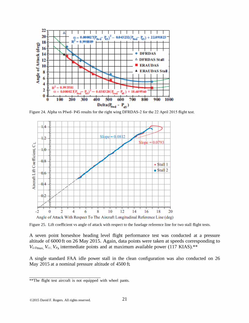
Figure 26 shows data from Stall 1 acquired using the DFRDAS-2. The absolute angle of attack
was determined using the calibration curve developed from the 4-leg GPS data shown in Figure
23. The Pfwd/P45 values calculated within the DFRDAS-2 during the stall flight test were used to
calculate the absolute angle of attack also within the DFRDAS-1. Figure 26 centers the initial stall
break at time zero, recovery was initiated at approximately three seconds and completed at
approximately five second, i.e., a total of approximately five seconds from stall break to recovery
completion. The maximum absolute angle of attack was approximately 19 1/2º while the minimum
angle of attack was approximately 6 1/2º. Figure 26 clearly indicates that the DFRDAS provides
adequate angle of attack information during stall recovery.
12. THE RESULTS OF THE 26/27 MAY 2015 FLIGHT TESTS
Two flight tests were conducted at Stevensville, Maryland (W29) on 26 and 27 May 2015. Again,
two separate DFRDAS systems were installed on the flight test aircraft. The left wing Alpha
System probe location and orientation was not changed from either the January or April 2015 flight
tests. The power law calibration curve (blue equation) from Figure 21 was implemented in the left
wing data acquisition system (DFRDAS-1) software. Code was included in the DFRDAS-1
software to calculate the absolute angle of attack from the power law calibration equation in real
time given Pfwd/P45.
Again the DFRDAS-2 data acquisition system was used to acquire data from the deferential
pressure angle of attack probe mounted at 38.9% local chord on the right wing. The orientation of
the right wing probe with respect to the wing lower surface was not change from the 22 April 2015
flight test. The software in the DFRDAS-2 used to determine Pfwd/P45 from the raw pressure sensor
output was not changed.
The raw values of Pfwd and P45 were output to data files. These values were used to independently calculate the ratio Pfwd/P45, and compare to those internally calculated within the DFRDAS.
©2015 David F. Rogers. All rights reserved.
21
Figure 24. Alpha vs Pfwd- P45 results for the right wing DFRDAS-2 for the 22 April 2015 flight test.
Figure 25. Lift coefficient vs angle of attack with respect to the fuselage reference line for two stall flight tests.
A seven point horseshoe heading level flight performance test was conducted at a pressure
altitude of 6000 ft on 26 May 2015. Again, data points were taken at speeds corresponding to
VL/Dmax, VCC, VPR intermediate points and at maximum available power (117 KIAS).**
A single standard FAA idle power stall in the clean configuration was also conducted on 26
May 2015 at a nominal pressure altitude of 4500 ft.
**The flight test aircraft is not equipped with wheel pants.
©2015 David F. Rogers. All rights reserved.
22
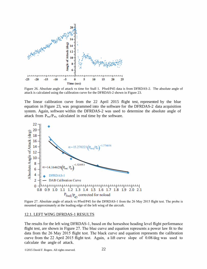
Figure 26. Absolute angle of attack vs time for Stall 1. Pfwd/P45 data is from DFRDAS-2. The absolute angle of
attack is calculated using the calibration curve for the DFRDAS-2 shown in Figure 23.
The linear calibration curve from the 22 April 2015 flight test, represented by the blue
equation in Figure 23, was programmed into the software for the DFRDAS-2 data acquisition
system. Again, software within the DFRDAS-2 was used to determine the absolute angle of
attack from Pfwd /P45, calculated in real time by the software.
Figure 27. Absolute angle of attack vs Pfwd/P45 for the DFRDAS-1 from the 26 May 2015 flight test. The probe is
mounted approximately at the leading edge of the left wing of the aircraft.
12.1. LEFT WING DFRDAS-1 RESULTS
The results for the left wing DFRDAS-1, based on the horseshoe heading level flight performance
flight test, are shown in Figure 27. The blue curve and equation represents a power law fit to the
data from the 26 May 2015 flight test. The black curve and equation represents the calibration
curve from the 22 April 2015 flight test. Again, a lift curve slope of 0.08/deg was used to
calculate the angle of attack.
©2015 David F. Rogers. All rights reserved.
23
The difference in angle of attack for a given value of Pfwd /P45 is likely a result of the method used
to determine both the angle of attack and Pfwd /P45. Specifically, the noload value was determined
by averaging 100 data points and was not changed, nor should it have been, for the two flight tests.
The 100 values for Pfwd /P45 for each leg of the 4-leg GPS horseshoe heading box pattern were
averaged and then the four averaged values averaged again. The four true airspeeds determined
from each of the triads of the 4-leg GPS horseshoe heading data were averaged to obtain the true
airspeed for each data point. In short, the values represented by the data points are an average of
an average. Finally, the calibration curve was determined by a ‘statistical’ fit to the averaged data.
The power law curves represent a reasonable approximation to the angle of attack for medium to
low angles of attack, i.e., for typical cruise and approach conditions. However, notice that near
stall both curves in Figure 27 become quite sensitive and tend to underestimate the angle of attack.
12.2. RIGHT WING DFRDAS-2 RESULTS
The results for the right wing DFRDAS-2 for the horseshoe heading flight test are shown in Figure
28. The angle of attack for the DFRDAS results was estimated using a lift curve slope of 0.080/deg.
The values of Pfwd /P45 are based on the individual values of Pfwd and P45 corrected for noload
(sensor bias) from the DFRDAS-2 angle of attack data acquisition system. Figure 28 shows the
angle of attack, α, plotted against Pfwd /P45. Again, as in the 22 April 2015 test, the variation is
linear. The blue equation in Figure 25 was programmed into the DFRDAS-2 and is shown here as
the black line and equation. The differences between the linear fits to the data represented by the
blue and black lines is attributed to the effect of averaging the averages discussed in Appendix D.
Some of the ‘scatter’ in the data is a result of ‘ringing’ in the pressure sensors. However, a
significant amount of the ‘scatter’ results from the continuous very small changes in angle of attack
made by the pilot in order to maintain constant airspeed and altitude without changing power or
trim during the data run.
12.3. RIGHT WING FLAPS 40º RESULTS
A four point 4-leg GPS horseshoe heading flight test was conducted at 6000 ft pressure altitude
with full flaps (nominally 40◦) extended. The results are shown in Figure 29. The flaps zero
calibration curve from Figure 28 is shown for comparison. Figure 29 again shows a linear
calibration curve with flaps extended. Figure 29 also shows that Pfwd /P45, for a given angle of
attack, is larger with flaps extended than without flaps extended. In addition, the slope of the
calibration curve is approximately twice that with 40º flaps extended than without flaps extended.
It is known from NACA airfoil data [ARR45] that flap extension beyond approximately 30◦
changes the lift curve slope. Additional flight tests at lower flap extensions may change the result
seen with 40◦ flap extension.
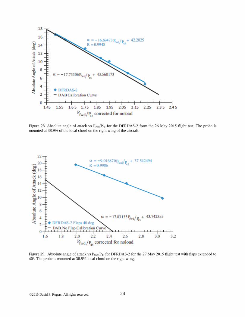
©2015 David F. Rogers. All rights reserved.
24
Figure 28. Absolute angle of attack vs Pfwd/P45 for the DFRDAS-2 from the 26 May 2015 flight test. The probe is
mounted at 38.9% of the local chord on the right wing of the aircraft.
Figure 29. Absolute angle of attack vs Pfwd/P45 for DFRDAS-2 for the 27 May 2015 flight test with flaps extended to
40º. The probe is mounted at 38.9% local chord on the right wing.
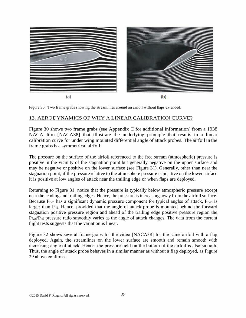
©2015 David F. Rogers. All rights reserved.
25
Figure 30. Two frame grabs showing the streamlines around an airfoil without flaps extended.
13. AERODYNAMICS OF WHY A LINEAR CALIBRATION CURVE?
Figure 30 shows two frame grabs (see Appendix C for additional information) from a 1938
NACA film [NACA38] that illustrate the underlying principle that results in a linear
calibration curve for under wing mounted differential angle of attack probes. The airfoil in the
frame grabs is a symmetrical airfoil.
The pressure on the surface of the airfoil referenced to the free stream (atmospheric) pressure is
positive in the vicinity of the stagnation point but generally negative on the upper surface and
may be negative or positive on the lower surface (see Figure 31). Generally, other than near the
stagnation point, if the pressure relative to the atmosphere pressure is positive on the lower surface
it is positive at low angles of attack near the trailing edge or when flaps are deployed.
Returning to Figure 31, notice that the pressure is typically below atmospheric pressure except
near the leading and trailing edges. Hence, the pressure is increasing away from the airfoil surface.
Because Pfwd has a significant dynamic pressure component for typical angles of attack, Pfwd is
larger than P45. Hence, provided that the angle of attack probe is mounted behind the forward
stagnation positive pressure region and ahead of the trailing edge positive pressure region the
Pfwd/P45 pressure ratio smoothly varies as the angle of attack changes. The data from the current
flight tests suggests that the variation is linear.
Figure 32 shows several frame grabs for the video [NACA38] for the same airfoil with a flap
deployed. Again, the streamlines on the lower surface are smooth and remain smooth with
increasing angle of attack. Hence, the pressure field on the bottom of the airfoil is also smooth.
Thus, the angle of attack probe behaves in a similar manner as without a flap deployed, as Figure
29 above confirms.
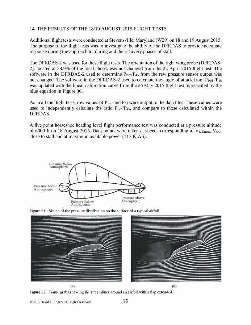
©2015 David F. Rogers. All rights reserved.
26
14. THE RESULTS OF THE 18/19 AUGUST 2015 FLIGHT TESTS
Additional flight tests were conducted at Stevensville, Maryland (W29) on 18 and 19 August 2015.
The purpose of the flight tests was to investigate the ability of the DFRDAS to provide adequate
response during the approach to, during and the recovery phases of stall.
The DFRDAS-2 was used for these flight tests. The orientation of the right wing probe (DFRDAS-
2), located at 38.9% of the local chord, was not changed from the 22 April 2015 flight test. The
software in the DFRDAS-2 used to determine Pfwd/P45 from the raw pressure sensor output was
not changed. The software in the DFRDAS-2 used to calculate the angle of attack from Pfwd /P45
was updated with the linear calibration curve from the 26 May 2015 flight test represented by the
blue equation in Figure 30.
As in all the flight tests, raw values of Pfwd and P45 were output to the data files. These values were
used to independently calculate the ratio Pfwd/P45, and compare to those calculated within the
DFRDAS.
A five point horseshoe heading level flight performance test was conducted at a pressure altitude
of 6000 ft on 18 August 2015. Data points were taken at speeds corresponding to VL/Dmax, VCC,
close to stall and at maximum available power (117 KIAS).
Figure 31. Sketch of the pressure distribution on the surface of a typical airfoil.
Figure 32. Frame grabs showing the streamlines around an airfoil with a flap extended.
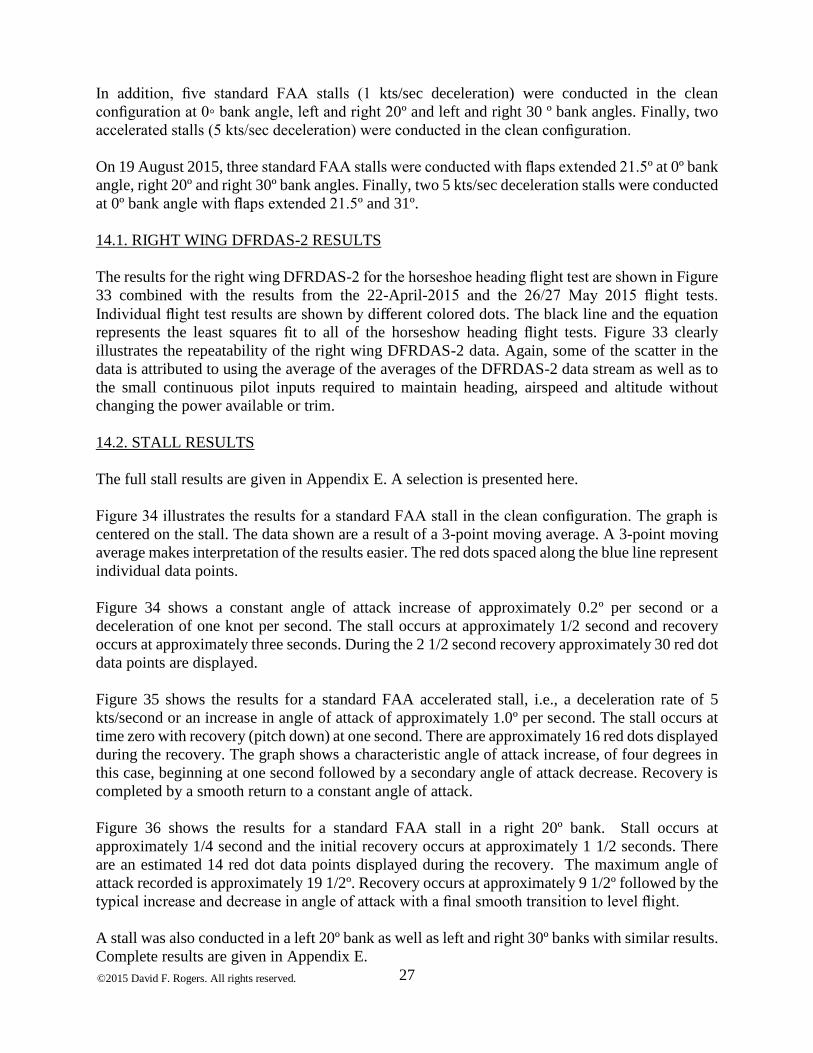
©2015 David F. Rogers. All rights reserved.
27
In addition, five standard FAA stalls (1 kts/sec deceleration) were conducted in the clean
configuration at 0◦ bank angle, left and right 20º and left and right 30 º bank angles. Finally, two
accelerated stalls (5 kts/sec deceleration) were conducted in the clean configuration.
On 19 August 2015, three standard FAA stalls were conducted with flaps extended 21.5º at 0º bank
angle, right 20º and right 30º bank angles. Finally, two 5 kts/sec deceleration stalls were conducted
at 0º bank angle with flaps extended 21.5º and 31º.
14.1. RIGHT WING DFRDAS-2 RESULTS
The results for the right wing DFRDAS-2 for the horseshoe heading flight test are shown in Figure
33 combined with the results from the 22-April-2015 and the 26/27 May 2015 flight tests.
Individual flight test results are shown by different colored dots. The black line and the equation
represents the least squares fit to all of the horseshow heading flight tests. Figure 33 clearly
illustrates the repeatability of the right wing DFRDAS-2 data. Again, some of the scatter in the
data is attributed to using the average of the averages of the DFRDAS-2 data stream as well as to
the small continuous pilot inputs required to maintain heading, airspeed and altitude without
changing the power available or trim.
14.2. STALL RESULTS
The full stall results are given in Appendix E. A selection is presented here.
Figure 34 illustrates the results for a standard FAA stall in the clean configuration. The graph is
centered on the stall. The data shown are a result of a 3-point moving average. A 3-point moving
average makes interpretation of the results easier. The red dots spaced along the blue line represent
individual data points.
Figure 34 shows a constant angle of attack increase of approximately 0.2º per second or a
deceleration of one knot per second. The stall occurs at approximately 1/2 second and recovery
occurs at approximately three seconds. During the 2 1/2 second recovery approximately 30 red dot
data points are displayed.
Figure 35 shows the results for a standard FAA accelerated stall, i.e., a deceleration rate of 5
kts/second or an increase in angle of attack of approximately 1.0º per second. The stall occurs at
time zero with recovery (pitch down) at one second. There are approximately 16 red dots displayed
during the recovery. The graph shows a characteristic angle of attack increase, of four degrees in
this case, beginning at one second followed by a secondary angle of attack decrease. Recovery is
completed by a smooth return to a constant angle of attack.
Figure 36 shows the results for a standard FAA stall in a right 20º bank. Stall occurs at
approximately 1/4 second and the initial recovery occurs at approximately 1 1/2 seconds. There
are an estimated 14 red dot data points displayed during the recovery. The maximum angle of
attack recorded is approximately 19 1/2º. Recovery occurs at approximately 9 1/2º followed by the
typical increase and decrease in angle of attack with a final smooth transition to level flight.
A stall was also conducted in a left 20º bank as well as left and right 30º banks with similar results.
Complete results are given in Appendix E.
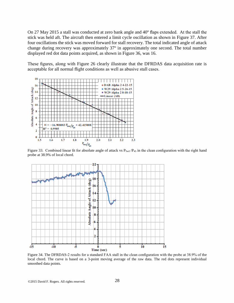
©2015 David F. Rogers. All rights reserved.
28
On 27 May 2015 a stall was conducted at zero bank angle and 40º flaps extended. At the stall the
stick was held aft. The aircraft then entered a limit cycle oscillation as shown in Figure 37. After
four oscillations the stick was moved forward for stall recovery. The total indicated angle of attack
change during recovery was approximately 37º in approximately one second. The total number
displayed red dot data points acquired, as shown in Figure 36, was 16.
These figures, along with Figure 26 clearly illustrate that the DFRDAS data acquisition rate is
acceptable for all normal flight conditions as well as abusive stall cases.
Figure 33. Combined linear fit for absolute angle of attack vs Pfwd /P45 in the clean configuration with the right hand
probe at 38.9% of local chord.
Figure 34. The DFRDAS-2 results for a standard FAA stall in the clean configuration with the probe at 38.9% of the
local chord. The curve is based on a 3-point moving average of the raw data. The red dots represent individual
smoothed data points.
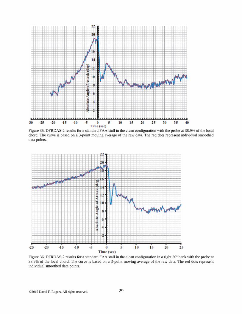
©2015 David F. Rogers. All rights reserved.
29
Figure 35. DFRDAS-2 results for a standard FAA stall in the clean configuration with the probe at 38.9% of the local
chord. The curve is based on a 3-point moving average of the raw data. The red dots represent individual smoothed
data points.
Figure 36. DFRDAS-2 results for a standard FAA stall in the clean configuration in a right 20º bank with the probe at
38.9% of the local chord. The curve is based on a 3-point moving average of the raw data. The red dots represent
individual smoothed data points.
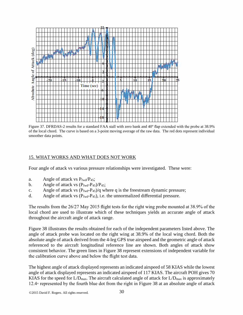
©2015 David F. Rogers. All rights reserved.
30
Figure 37. DFRDAS-2 results for a standard FAA stall with zero bank and 40º flap extended with the probe at 38.9%
of the local chord. The curve is based on a 3-point moving average of the raw data. The red dots represent individual
smoother data points.
15. WHAT WORKS AND WHAT DOES NOT WORK
Four angle of attack vs various pressure relationships were investigated. These were:
a. Angle of attack vs Pfwd/P45;
b. Angle of attack vs (Pfwd-P45)/P45;
c. Angle of attack vs (Pfwd-P45)/q where q is the freestream dynamic pressure;
d. Angle of attack vs (Pfwd-P45), i.e. the unnormalized differential pressure.
The results from the 26/27 May 2015 flight tests for the right wing probe mounted at 38.9% of the
local chord are used to illustrate which of these techniques yields an accurate angle of attack
throughout the aircraft angle of attack range.
Figure 38 illustrates the results obtained for each of the independent parameters listed above. The
angle of attack probe was located on the right wing at 38.9% of the local wing chord. Both the
absolute angle of attack derived from the 4-leg GPS true airspeed and the geometric angle of attack
referenced to the aircraft longitudinal reference line are shown. Both angles of attack show
consistent behavior. The green lines in Figure 38 represent extensions of independent variable for
the calibration curve above and below the flight test data.
The highest angle of attack displayed represents an indicated airspeed of 58 KIAS while the lowest
angle of attack displayed represents an indicated airspeed of 117 KIAS. The aircraft POH gives 70
KIAS for the speed for L/Dmax. The aircraft calculated angle of attack for L/Dmax is approximately
12.4◦ represented by the fourth blue dot from the right in Figure 38 at an absolute angle of attack
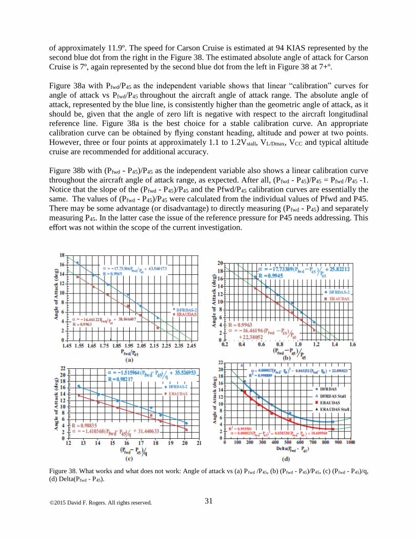
©2015 David F. Rogers. All rights reserved.
31
of approximately 11.9º. The speed for Carson Cruise is estimated at 94 KIAS represented by the
second blue dot from the right in the Figure 38. The estimated absolute angle of attack for Carson
Cruise is 7º, again represented by the second blue dot from the left in Figure 38 at 7+º.
Figure 38a with Pfwd/P45 as the independent variable shows that linear “calibration” curves for
angle of attack vs Pfwd/P45 throughout the aircraft angle of attack range. The absolute angle of
attack, represented by the blue line, is consistently higher than the geometric angle of attack, as it
should be, given that the angle of zero lift is negative with respect to the aircraft longitudinal
reference line. Figure 38a is the best choice for a stable calibration curve. An appropriate
calibration curve can be obtained by flying constant heading, altitude and power at two points.
However, three or four points at approximately 1.1 to 1.2Vstall, VL/Dmax, VCC and typical altitude
cruise are recommended for additional accuracy.
Figure 38b with (Pfwd - P45)/P45 as the independent variable also shows a linear calibration curve
throughout the aircraft angle of attack range, as expected. After all, (Pfwd - P45)/P45 = Pfwd /P45 -1.
Notice that the slope of the (Pfwd - P45)/P45 and the Pfwd/P45 calibration curves are essentially the
same. The values of (Pfwd - P45)/P45 were calculated from the individual values of Pfwd and P45.
There may be some advantage (or disadvantage) to directly measuring (Pfwd - P45) and separately
measuring P45. In the latter case the issue of the reference pressure for P45 needs addressing. This
effort was not within the scope of the current investigation.
Figure 38. What works and what does not work: Angle of attack vs (a) Pfwd /P45, (b) (Pfwd - P45)/P45, (c) (Pfwd - P45)/q,
(d) Delta(Pfwd - P45).
©2015 David F. Rogers. All rights reserved.
32
Figure 38c with (Pfwd - P45)/q as the independent variable shows a linear calibration curve. Recall
that (Pfwd - P45) is the differential pressure and q is the freestream dynamic pressure. Specifically,
q is not the dynamic pressure derived from the pitot-static system. This is a subtle, but important,
point. Most aircraft pitot-static systems require correction at low speed/high angle of attack near
stall because of errors in either the pitot tube and/or the static pressure readings. If these corrections
are not incorporated into the angle of attack system, it is unlikely that a linear calibration with (Pfwd
- P45)/q results. Similar results may be expected for other differential pressure systems.
Figure 38d with simply the unnormalized differential pressure (Pfwd - P45) as the independent
variable does not show a linear calibration for angle of attack vs (Pfwd - P45). The best fit is a second
degree polynomial as shown by the red and blue lines in Figure 38d. The green lines represent
extensions of the polynomial fits to both lower and higher angles of attack. In the low angle of
attack (high speed) regime the polynomial fit “turns up” which results in an ambiguous angle of
attack. If simple unnormalized differential pressure is used as the independent variable, a multi-
point chord wise approximation using a near stall speed, VPRmin, VL/Dmax, VCC, normal cruise speed
and high speed cruise as suggested by Rogers [ROG13] yields acceptable results.
16. CONCLUSIONS
a. A differential pressure based COTS angle of attack data acquisition system was designed,
successfully reduced to practice, wind tunnel tested and flight tested.
b. The accuracy of the differential pressure angle of attack system was determined to be 1/4º
to 1/2º.
c. A data rate of 17 samples/sec or better was achieved during all the flight tests including
during all phases of FAA standard and accelerated stalls, approach to stall, full stall and
stall recovery.
d. Use of the local ambient pressure as the reference for the differential pressure sensors was
confirmed in practice.
e. The repeatability of the data from the COTS data acquisition system was proven in flight
test.
f. A calibration curve based on the ratio Pfwd/P45 is linear throughout the aircraft angle of
attack range if the probe is mounted in an inspection port on the bottom of the wing the
center of which is located between an estimated 25% to an estimated 60% of the local wing
chord. Similar results may be expected for other differential pressure systems.
g. The linear calibration curve results because; on the lower surface of the wing, the flow
remains attached and varies smoothly in the pressure field between the wing lower surface
and the far field static (atmospheric) pressure below the wing throughout the entire aircraft
angle of attack range including stall with and without a deflected flap.
h. A physics based determination of angle of attack was successful, provided that a reasonably
accurate aircraft lift curve is determined. Calculation of the lift curve slope was within
0.01/deg of the value determined by flight test using an alpha/beta probe.
i. With the angle of attack probe mounted at the leading edge of the local chord, a power law
calibration curve cast as angle of attack vs Pfwd/P45 provides a better fit to the data than a
parabolic or linear fit. For a limited range of high angles of attack near stall a linear fit to
the data provides adequate accuracy. However, accuracy at low angles of attack, such as
required by cruise, is poor. Hence, systems, similar to that tested, mounted near the leading
edge and using a linear calibration are basically only stall warning devices.

©2015 David F. Rogers. All rights reserved.
33
j. Using unnormalized differential pressure (Pfwd - P45) does not provide adequate accuracy
throughout the aircraft angle of attack range. This technique is dynamic pressure
dependent. Similar results may be expected for other differential pressure systems.
For a limited range of high angles of attack near stall a linear fit to the data provides
adequate accuracy. However, accuracy at low angles of attack, such as required by cruise,
is poor. Hence, systems similar to that tested, using a linear calibration are basically only
stall warning devices.
k. Normalizing the differential pressure with aircraft dynamic pressure is impractical in the
aftermarket because of the necessity to include the aircraft high angle of attack (low speed)
pitot-static correction to achieve the required accuracy.
17. SUGGESTED FUTURE WORK
a. More carefully determine the acceptable local chord range for probe location. Conduct
flight tests to confirm proper operation from 25% chord to 60% chord.
b. Determine the sensitivity of the probe to flap deflection, e.g., flaps 10º, 20º and 30º.
c. Conduct a literature search to see if studies of the lower surface far field exist.
d. Explore the behavior of the pressure field between the lower surface of the wing and the
far field using PIV, CFD and/or flight test studies.
e. Study the effect of “ringing/jitter” in angle of attack display including the ergonomic effect
on pilot acceptance and interpretation as well as techniques for reducing and/or eliminating
the effect.
f. The variation with distance from the wing of the pressure field between the lower surface
of the wing and the far field is little known (see c. above), hence the distance between the
Pfwd and P45 ports on the angle of attack probe may significantly influence the performance
of the probe. Use CFD, wind tunnel tests and/or flight tests to explore this effect on probe
performance.
g. Conduct tests of alternate display configurations for presenting angle of attack information
to the pilot.
h. Relax the original requirement for installing the probe in an EXISTING inspection plate.
i. Convey to the developers that only PFWD/P45, or (PFWD - P45)/P45 correctly (linear)
normalizes the dynamic pressure effect.
j. Convey to the developers that using only PFWD - P45 does NOT yield an accurate angle of
attack indication. It is ONLY a stall warning device.
k. Convey to the developers that, in their installation instructions, the probe should be
mounted on the wing opposite to the standard stall warning device to provide stall warning
in both a left and right hand turn.
l. Develop an Advisory Circular on differential pressure transducer based angle of attack
data acquisition systems.
18. REFERENCES
ARR45 Abbott, I.H., von Doenhoff, A.E. and Stivers, L.S. Jr., “Summary of Airfoil
Data”, NACA TR-824, 1945 also available as Abbott, I.H. and von Doenhoff,
A.E., “Theory of Wing Sections Including a Summary of Airfoil Data”, Dover
Publications, INC., New York, 1949, 1959.

©2015 David F. Rogers. All rights reserved.
34
And89 Anderson, John D. Jr., Introduction to Flight, McGraw-Hill Publishing
Company, New York, 1989.
ARE09 Arend, D. J. and Saunders, J. D., “An Experimental Evaluation of the
Performance of Two Combination Pitot Pressure Probes,” NASA Technical
Paper TP-2009-215632M, October 2009.
BENa Online bending mount calculator http://bendingmomentdiagram.com/
BOS85 BMP085 Digital Pressure Sensor Data Sheet, Bosch Sensortec Inc. USA, 2400
Geng Road - Ste. 200, Palo Alto, CA, 94303.
CAR82 Carson, B. H., “Fuel Efficiency of Small Aircraft,” Journal of Aircraft, Vol.
19, 1982, pp. 473–479.
CFR “Limit Maneuvering Load Factors”, sourced from
http://www.gpo.gov/fdsys/granule/CFR-2011-title14- vol1/CFR-2011-title14-
vol1-sec23-337.
CFDa Solid Works Fluid Flow Analysis, available at www.solidworks.com
COR53 Corning, G., “Supersonic and Subsonic Airplane Design”, 2nd Edition, Third
Printing, 1953.
FEAa Solid Works Finite Element Analysis, available at www.solidworks.com
FOX95 Fox, D., “Is Your Speed True?”, Kitplanes, Feb. 1995, pp. 49–50.
GAR34 Garrick, I.E., “Determination of the Theoretical Pressure Distribution for
Twenty Airfoils,” NACA TR-465, 1934.
GRA58 Gracey, W, “Summary of Methods of Measuring Angle of Attack on Aircraft,”
NACA TN-4351, August 1958.
LEW97 Lewis, G., “A Flight Test Technique Using GPS for Position Error Correction
Testing,” Cockpit, Jan.– March 1997, pp. 20–24
MIL8 MILSTD-882C, “Military Standard System Safety Program Requirements,”
January 1993.
MS45 MS4525DO Data Sheet, Measurement Specialties Inc., 1000 Lucas Way,
Hampton, VA 23666, www.meas-spec.com.
NACA38 NACA, “Aerodynamics: Airfoil Cambers, Flaps, Slots-Slats and Drag
“Smoke Lifts”, National Advisory Committee for Aeronautics, circa 1938,
Langley Research Laboratory sourced from YouTube
https://www.youtube.com/watch?v=qeMQvDoDWk .
P&H49 Perkins, C.D. and Hage, R. E., “Airplane Performance Stability and
Control”, John Wiley & Sons, New York, 1949.
POH Cessna Model 182Q Pilot’s Operating Handbook, Cessna Aircraft Corporation,
1 Cessna Blvd, Wichita, KA 67215.
ROG02 Rogers, D. F., “An Engineering Flight Test Course Emphasizing
Flight Mechanics Concepts”, Journal of Aircraft, Vol. 39, No.1, Jan–Feb.
2002, pp. 79–83.
ROG13 Rogers, David F., “Investigation of a General-Aviation Differential Pressure
Angle-of-Attack Probe,”
Journal of Aircraft, Vol. 50, No. 5, Sept–Oct. 2013, pp. 1668-1671.
SAD11 Letter from the FAA Small Airplane Directorate, Kansas City, KS, to DepotStar
Inc., dated 15 December 2011.
WOO63 Wood, K.D., “Aerospace Vehicle Design, Vol. 1, Aircraft Design”,
Johnson Publishing Company, Boulder, CO, 1963.
©2015 David F. Rogers. All rights reserved.
35
APPENDIX A. DETAILS FOR THE ARDUINO BASED COTS SYSTEM
The COTS data acquisition system consists of the Arduino UNO, two Measurement Specialties
MS4525 0–1 psi differential pressure sensors, a Bosch BMP085 altitude/pressure sensor and
various resistors and capacitors, as detailed in the block diagram below. The pressure sensors,
Bosch BMP085 (or BMP180) and the small parts are mounted on a Proto shield which attaches to
the UNO. The pinouts are also given in the block diagram below.
Figure A-1. Block diagram for Arduino DFRDAS data acquisition system.
©2015 David F. Rogers. All rights reserved.
36
A list of parts, sources and costs is given below in Table A-1.
Table A-1. Parts List and Costs—DFRDAS Data Acquisition System.
Item Mfr Mfr No. Qty Source Cost 1 Arduino UNO R3
DIP Edition Arduino A000066 1 Newark Elec. $22.92
2 Proto Shield for Arduino UNO
STR 104B2P 1 Adafruit $5.00
3 Bosch GY-65 (BMP085 or BMP180)
Bosch GY-65/BMP085 1 Component City $8.75
4 MS4525DO Measurement Specialties
4525DO - DS 5AI001DP
2 Servoflo Corp $42.00
5 CD4066BE Texas Instruments CD4066BE 1 Newark Elec. $0.48
6 Capacitor Alum Elec 0.1 microF 35V 20%
Multicomp MCMHR63V104MAX7 2 Newark Elec. $0.45
7 Cable USB 3FT Multicomp SPC20065 1 Newark Elec. $2.31
8 Resistor, Carbon Film 4.7k Ohm 0.25 W 5%
Multicomp MCF 0.25W 4K7 2 Newark Elec. $0.60
9 Tubing Fitting Avery Tools SA-F1 2 Straight Female $9.42
10 Adapter Cole-Parmer EW-06365-42 2 1/8” Male Pipe to 1/8” Barb
$0.92
The Arduino sketch (program) begins with declaration of the global variables followed by setting
up the pins allowing communication with the hardware. The main loop first gets the atmospheric
pressure from the Bosch BMP085 or BMP180. Because only MS4525 sensors with a common I2C
address were available, it was necessary to multiplex accessing the two MS4525 pressure sensors
for Pfwd and P45. The Pfwd and P45 pressure values are acquired as raw counts in the range of 0 to
16383. These values are corrected by subtracting the ‘noload’ values corresponding to zero
differential pressure. The ratio Pfwd/P45 is then calculated using the ‘noload’ corrected Pfwd and P45
values. The angle of attack, α, is then determined from the calibration equation. Finally, the result
is either printed or displayed as required.
©2015 David F. Rogers. All rights reserved.
37
Figure A-2. Block diagram for Arduino DFRDAS data acquisition system sketch (program).
©2015 David F. Rogers. All rights reserved.
38
The Arduino code listing below is for the DFRDAS angle of attack data acquisition system
used in the flight tests. The linear calibration ‘curve’ is based on the composite flight test curve
give in Figure 41. During those flight tests the probe was mounted at 38.9% of the local wing
chord. The calibration ‘curve’ should be adjusted for any other wing location (see lines 95 &
96). The noload values should be adjusted for individual sensors (see lines 98 & 99). The probe
location should be between an estimated 25% and 60% of the local wing chord outboard of the
wing flap.
ArduinoListing 1 // Name: Bar_and_Diff_pressure_V1_4_2.ino
2 // Version: 1_4_2
3 // Date: 29 July 2015
4 // Author: Francisco Rodriguez
5 // Calibration: Alpha2 Linear From DAB 5-26/27/2015
6
7 // Arduino 1.0+ Only
8
9 /* Based largely on code by Jim Lindblom
10
11 // Bar_and_Diff_pressure_V1_4_2
12
13 Get pressure, altitude, and temperature from the BMP085.
14 Serial.print it out at 9600 baud to serial monitor.
15 */
16
17 #include <Wire.h>
18
19 #define BMP085_ADDRESS 0x77 // I2C address of BMP085
20
21 const unsigned char OSS = 0; // Oversampling Setting
22
23 // Calibration values
24 int ac1;
25 int ac2;
26 int ac3;
27 unsigned int ac4;
28 unsigned int ac5;
29 unsigned int ac6;
30 int b1;
31 int b2;
32 int mb;
33 int mc;
34 int md;
35 float pressurepsi;
36 float altitudefeet;
37 float temperaturec;
38 int ver = 142;
39
40
41 // Definitions for Delta Pressure sensor
42
43 int press_address = 40; //1001000 written as decimal number
44 int reading = 0;
45 int mask = 63; //(0 0 1 1 1 1 1 1 )

©2015 David F. Rogers. All rights reserved.
39
46 int maskstatus = 192; //(1 1 0 0 0 0 0 0 )
47 int Status;
48 float deltapressure;
49 float deltapressure1;
50 float deltapressure2;
51
52 // Definitions for Alpha Calculations
53
54 float pfwdnoload, p45noload;
55 float pfwd, p45;
56 float pfwd_p45, Alpha; // pfwd_p45 is Pfwd/P45
57 float pfwdcorr, p45corr, Dtarepfwd,Dtarep45,deltanoloadpfwd;
58 float deltanoloadp45, psi_count;
59 float A, B;
60
61 // Definitions for LED Control
62
63 int led13 = 13;
64 int num1 = 0;
65 int led = 1;
66
67 int unit = 1; // 1 = unit1 selected, 2 = unit2 selected
68
69 // b5 is calculated in bmp085GetTemperature(...)
70 // the b5 variable is also used in bmp085GetPressure(...)
71 // so ...Temperature(...) must be called before ...Pressure(...)
72
73 long b5;
74
75 // Definition of output control
76
77 const int unit1 = 8;
78 const int unit2 = 9;
79
80
81 void setup(){ // Setup loop
82 Serial.begin(9600);
83 Wire.begin();
84
85 pinMode (unit1, OUTPUT); // set pin 8 control for sensor 1
86 pinMode (unit2, OUTPUT); // set pin 9 control for sensor 2
87 digitalWrite( unit1, LOW); // set both units off line
88 digitalWrite( unit2, LOW);
89
90 //----------------Calibration FOR ALPHA 2 ------------------
91
92 //-- ALPHA 2 Right Wing Flight Test Calibration Curve
93 //-- Linear from DAB 5-26/27-2015 Alpha = A*(Pfwd/P45) + B
94
95 A = -16.908083; // These values must be adjusted for individual
96 B = 42.415008; // probes and probe locations
97
98 pfwdnoload = 8162.9; //counts Adjust these values for
99 p45noload = 8186.6; //counts the individual sensors
100
101 //-------NOTE THE BMP085 IS NOT ACTUALLY NEEDED--------------
102 //-------THE SENSOR CAN BE REMOVED FROM THE DFRDAS-----------

©2015 David F. Rogers. All rights reserved.
40
103 //-------ALONG WITH THE ASSOCIATED CODE----------------------
104
105 bmp085Calibration();
106 pinMode(led13, OUTPUT);
107 } // end setup loop
108
109 void loop() // Main loop
110 {
111 float temperature = bmp085GetTemperature(bmp085ReadUT()); //MUST be called first
112 float pressure = bmp085GetPressure(bmp085ReadUP());
113 float atm = pressure / 101325; // "Standard Atmosphere Sea Level Pressure"
114 float altitude = calcAltitude(pressure); // Uncompensated calculation - in Meters
115
116 // Various alternative possibilities for output from the BMP085
117
118 // Serial.print("Barometric Pressure = ");
119 pressurepsi = pressure * 0.000145037738; // convert from Pa to psi
120 altitudefeet = altitude * 3.280839895; // convert altitude from meters to feet
121 // Serial.print(pressurepsi, 6);
122 // Serial.println("psi");
123
124 // Serial.print("Barometric Pressure = ");
125 // pressurepsi = pressure * 0.000295; // convert from Pa to inHg
126 // Serial.print(pressurepsi,6);
127 // Serial.println(" inHg");
128
129 // Serial.print("Altitude = ");
130 // altitude = altitude * 3.2808; // convert from Pa to inHg
131 // Serial.print(altitude,2);
132 // Serial.println(" feet");
133 // -----------------------------------------------------------------------------------
134 // Serial.print(pressurepsi);
135
136 Serial.print(altitudefeet,2);
137 Serial.print(",");
138
139 if ( num1 > 5 ) // Discard initil 5 inputs for stability
140 {
141 led =-led;
142 num1 =0;
143
144 // Multiplex the two MS4525 pressure sensors
145
146 if (led < 0)
147 {
148 digitalWrite(led13,HIGH);
149 }
150 else
151 {
152 digitalWrite(led13,LOW);
153 }
154
155 }
156
157 num1 =num1+1;
158
159 //-------------------------------------------------

©2015 David F. Rogers. All rights reserved.
41
160 // Get Differential Pressure from unit 1
161
162 digitalWrite(unit1,HIGH );
163 unit=1;
164 float pfwd = MS4525Getpressure(unit); // Get Differential Pressure from unit 1
165 digitalWrite( unit1, LOW);
166
167 //pfwd =7814.83; // TEST =========================
168
169 Serial.print( pfwd); // Print raw counts
170 Serial.print(",");
171
172 pfwdcorr = pfwd - pfwdnoload; // Account for no load
173
174 // Serial.print( pfwdcorr, 6); // Debuggign
175 // Serial.print(" , ");
176
177
178 //-------------------------------------------------
179 // Get Differential Pressure from unit 2
180 digitalWrite(unit2,HIGH );
181
182 unit=2;
183 float p45 = MS4525Getpressure(unit); // Get Differential Pressure from unit 2
184 digitalWrite( unit2, LOW);
185
186 //p45 =7926.78; // TEST============================
187
188 Serial.print( p45); // Print raw counts
189 Serial.print(",");
190
191 p45corr = p45 - p45noload; // Account for noload
192
193 // Serial.print( p45corr,6); // Debugging
194 // Serial.print(" , ");
195
196 digitalWrite(unit2,LOW);
197
198 Serial.flush(); // Clear serial port
199 // get values again.
200
201 // pfwdcorr=1; // TEST=============================
202 // p45corr=-2; // TEST=============================
203
204
205 pfwd_p45 = pfwdcorr/p45corr;
206
207 // Serial.print(pfwd_p45,10);
208 // Serial.print(" ------, ");
209
210 //----------------TEST------------------------------
211 // pfwd_p45 = 2.1;
212 //----------------END TEST--------------------------
213
214 Serial.print(pfwd_p45,5);
215 Serial.print(" , ");
216

©2015 David F. Rogers. All rights reserved.
42
217 //----- Calculate Alpha From Pfwd/P45 --------------
218
219 Alpha = A*(pfwd_p45) + B;
220
221 Serial.print(Alpha);
222 Serial.print(" , ");
223
224 Serial.print(pfwdnoload);
225
226 Serial.print(" , ");
227 Serial.print(p45noload);
228
229 Serial.print(" , V=");
230 Serial.println(ver);
231
232 // delay(1000); // Debugging
233 // Serial.print("\n");
234
235
236 } // End of main loop
237
238 // Stores all of the bmp085’s calibration values into global variables
239 // Calibration values are required to calculate temp and pressure
240 // This function should be called at the beginning of the program
241
242 void bmp085Calibration()
243 {
244 ac1 = bmp085ReadInt(0xAA);
245 ac2 = bmp085ReadInt(0xAC);
246 ac3 = bmp085ReadInt(0xAE);
247 ac4 = bmp085ReadInt(0xB0);
248 ac5 = bmp085ReadInt(0xB2);
249 ac6 = bmp085ReadInt(0xB4);
250 b1 = bmp085ReadInt(0xB6);
251 b2 = bmp085ReadInt(0xB8);
252 mb = bmp085ReadInt(0xBA);
253 mc = bmp085ReadInt(0xBC);
254 md = bmp085ReadInt(0xBE);
255 }
256
257 // Calculate temperature in deg C
258
259 float bmp085GetTemperature(unsigned int ut){
260 long x1, x2;
261
262 x1 = (((long)ut - (long)ac6)*(long)ac5) >> 15;
263 x2 = ((long)mc << 11)/(x1 + md);
264 b5 = x1 + x2;
265
266 float temp = ((b5 + 8)>>4);
267 temp = temp /10;
268
269 return temp;
270 }
271
272 // Calculate pressure retrieved.
273 // Calibration values must be known.
©2015 David F. Rogers. All rights reserved.
43
274 // b5 is also required so bmp085GetTemperature(...) must be called first.
275 // Value returned is pressure in units of Pa.
276
277 long bmp085GetPressure(unsigned long up){
278 long x1, x2, x3, b3, b6, p;
279 unsigned long b4, b7;
280
281 b6 = b5 - 4000;
282
283 // Calculate B3
284 x1 = (b2 * (b6 * b6)>>12)>>11;
285 x2 = (ac2 * b6)>>11;
286 x3 = x1 + x2;
287 b3 = (((((long)ac1)*4 + x3)<<OSS) + 2)>>2;
288
289 // Calculate B4
290 x1 = (ac3 * b6)>>13;
291 x2 = (b1 * ((b6 * b6)>>12))>>16;
292 x3 = ((x1 + x2) + 2)>>2;
293 b4 = (ac4 * (unsigned long)(x3 + 32768))>>15;
294
295 b7 = ((unsigned long)(up - b3) * (50000>>OSS));
296 if (b7 < 0x80000000)
297 p = (b7<<1)/b4;
298 else
299 p = (b7/b4)<<1;
300
301 x1 = (p>>8) * (p>>8);
302 x1 = (x1 * 3038)>>16;
303 x2 = (-7357 * p)>>16;
304 p += (x1 + x2 + 3791)>>4;
305
306 long temp = p;
307 return temp;
308 }
309
310 // Read 1 byte from the BMP085 at ’address’
311
312 char bmp085Read(unsigned char address)
313 {
314 unsigned char data;
315
316 Wire.beginTransmission(BMP085_ADDRESS);
317 Wire.write(address);
318 Wire.endTransmission();
319
320 Wire.requestFrom(BMP085_ADDRESS, 1);
321 while(!Wire.available())
322 ;
323
324 return Wire.read();
325 }
326
327 // Read 2 bytes from the BMP085
328 // First byte will be from ’address’
329 // Second byte will be from ’address’+1
330
©2015 David F. Rogers. All rights reserved.
44
331 int bmp085ReadInt(unsigned char address)
332 {
333 unsigned char msb, lsb;
334
335 Wire.beginTransmission(BMP085_ADDRESS);
336 Wire.write(address);
337 Wire.endTransmission();
338
339 Wire.requestFrom(BMP085_ADDRESS, 2);
340 while(Wire.available()<2)
341 ;
342 msb = Wire.read();
343 lsb = Wire.read();
344
345 return (int) msb<<8 | lsb;
346 }
347
348 // Read the uncompensated temperature value
349
350 unsigned int bmp085ReadUT(){
351 unsigned int ut;
352
353 // Write 0x2E into Register 0xF4
354 // This requests a temperature reading
355 Wire.beginTransmission(BMP085_ADDRESS);
356 Wire.write(0xF4);
357 Wire.write(0x2E);
358 Wire.endTransmission();
359
360 // Wait at least 4.5ms
361 delay(5); // Wait 5 ms
362
363 // Read two bytes from registers 0xF6 and 0xF7
364 ut = bmp085ReadInt(0xF6);
365
366 return ut;
367 }
368
369 // Read the uncompensated pressure value
370
371 unsigned long bmp085ReadUP(){
372
373 unsigned char msb, lsb, xlsb;
374 unsigned long up = 0;
375
376 // Write 0x34+(OSS<<6) into register 0xF4
377 // Request a pressure reading w/ oversampling setting
378 Wire.beginTransmission(BMP085_ADDRESS);
379 Wire.write(0xF4);
380 Wire.write(0x34 + (OSS<<6));
381 Wire.endTransmission();
382
383 // Wait for conversion, delay time dependent on OSS
384 delay(2 + (3<<OSS));
385
386 // Read register 0xF6 (MSB), 0xF7 (LSB), and 0xF8 (XLSB)
387 msb = bmp085Read(0xF6);

©2015 David F. Rogers. All rights reserved.
45
388 lsb = bmp085Read(0xF7);
389 xlsb = bmp085Read(0xF8);
390
391 up = (((unsigned long) msb << 16) | ((unsigned long) lsb << 8) | (unsigned long) xlsb) >> (8-OSS);
392 //Serial.print(up);
393 //Serial.print(" , ");
394 return up;
395 }
396
397 void writeRegister(int deviceAddress, byte address, byte val) {
398 Wire.beginTransmission(deviceAddress); // start transmission to device
399 Wire.write(address); // send register address
400 Wire.write(val); // send value to write
401 Wire.endTransmission(); // end transmission
402 }
403
404 int readRegister(int deviceAddress, byte address){
405
406 int v;
407 Wire.beginTransmission(deviceAddress);
408 Wire.write(address); // register to read
409 Wire.endTransmission();
410
411 Wire.requestFrom(deviceAddress, 1); // read a byte
412
413 while(!Wire.available()) {
414 // waiting
415 }
416
417 v = Wire.read();
418 return v;
419 }
420
421 float calcAltitude(float pressure){
422
423 float A = pressure/101325;
424 float B = 1/5.25588;
425 float C = pow(A,B);
426 C = 1 - C;
427 C = C /0.0000225577;
428
429 return C;
430 }
431
432 // Get Delta Pressure from MS4525 ---------------------------------------
433
434 //Reads Differential Pressure from I2C Ms4525 sensor
435 //
436 float MS4525Getpressure(int unit){
437 deltapressure =0;
438
439 //Send a request
440 //Start talking to the device at the specified address
441 Wire.beginTransmission(press_address);
442 //Send a bit asking for register zero, the data register
443 Wire.write(0);
444 //Complete Transmission

©2015 David F. Rogers. All rights reserved.
46
445 Wire.endTransmission();
446
447 //Request 2 Byte from the specified address
448 Wire.requestFrom(press_address, 2);
449 //wait for response for 2 bytes
450
451 if(2 <=Wire.available())
452 {
453 reading = Wire.read(); // byte 1
454 //Status = reading & maskstatus; // check status
455 //Status = Status >>6;
456 //Serial.println(Status);
457
458 //if ( Status <= 0)
459 //{
460 reading = reading & mask;
461
462 reading = reading << 8; //
463
464 reading |= Wire.read(); // read byte 2
465 //Serial.print(reading);
466 //Serial.print(",");
467 deltapressure =reading;
468 //deltapressure = deltapressure/16383 - .5;
469
470 // Serial.println(pressure,4);
471 // }
472 }
473 //delay(50);
474 return(deltapressure);
475 }

©2015 David F. Rogers. All rights reserved.
47
APPENDIX B. MECHANICAL DRAWINGS, GENERAL ASSEMBLY, GROUND AND
FLIGHT TESTING
The following pages contain mechanical drawings for the right wing tip air data boom. This
installation is intended for Cessna 182 - N721A. The drawings represent three boom sections, three
mounting blocks, three boom straps, and three L brackets, shown in Figure B-1. The L brackets
are attached to the right wing tip rib using rivets per AC43.13-2B.
The blocks attach to the L brackets through the aircraft skin. The top of each block has a nut plate
installed over each of the four block holes. Blocks are fastened to the nut plates with AN3 bolts.
Straps are fasted to blocks with 10-32 in x 2 3/4 in bolts and associated hardware. The two most
aft boom tubes are constrained with one 10-32 in x 2 3/4 in bolt and associated hardware, seen in
Figures B-2 and B-3. The two swivel head boom segment and the middle boom tube are
constrained with one 10-32 in x 2 1/4 in bolt and associated hardware shown in Figures B-6 and
B-7.
Figure B-1. Isometric view.
Figure B-2. Side view.
Figure B-3. Front view.
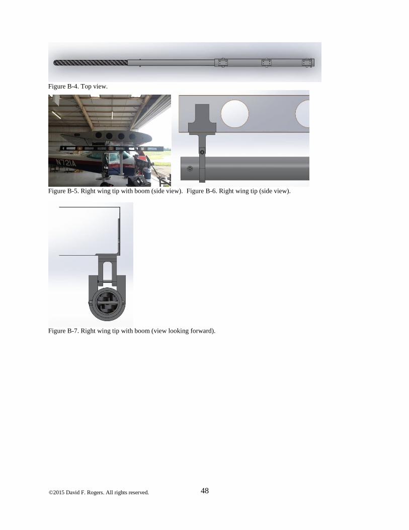
©2015 David F. Rogers. All rights reserved.
48
Figure B-4. Top view.
Figure B-5. Right wing tip with boom (side view). Figure B-6. Right wing tip (side view).
Figure B-7. Right wing tip with boom (view looking forward).

©2015 David F. Rogers. All rights reserved.
49
Figure B-8. Angle of attack data boom.
STRUCTURAL ANALYSIS OVERVIEW
Flight test booms are exposed to various loads during in-flight operations. The purpose of this test
is to physically test the boom structural behavior on the ground. The boom is designed to withstand
a 4.4g in-flight load. Details of the design and analysis are not included in this report.
The boom, shown in Figure B-8, is modeled with a swivel head at the tip, which weighs
approximately 1 lb, and four sections with different distributed loads. The first section starting at
the tip is made of carbon fiber, the second section consists of aluminum and carbon fiber and the
remaining sections are made of aluminum. Note that sections are superimposed, which has been
considered in the analysis. The boom is attached to the wing with three hinges. Inside the wing,
brackets, stiffeners, and shims are used to strengthen the outboard wing rib and skin. In Figure B-
9, the distributed loads for each section are shown as well as the point load due to the tip probe.
The point and distributed loads represent a 4.4g in-flight load. The assumptions for the finite
element analysis (FEA) are shown at the top right of Figure B-9.
Ground tests used point loads representative of the resultant forces in order to reproduce the shear
and bending moment diagram shown in Figures B-11 and B-12. All point loads were rounded up
to the closest available weight. The theoretical and actual loads are described in Figure B-10. Note
that the actual loads are the ones in parentheses (all loads were conservative).
Figure B-9. Data boom free body diagram.
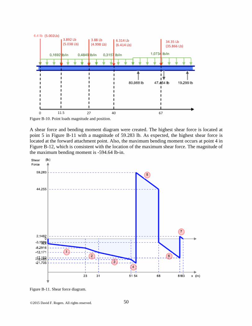
©2015 David F. Rogers. All rights reserved.
50
Figure B-10. Point loads magnitude and position.
A shear force and bending moment diagram were created. The highest shear force is located at
point 5 in Figure B-11 with a magnitude of 59.283 lb. As expected, the highest shear force is
located at the forward attachment point. Also, the maximum bending moment occurs at point 4 in
Figure B-12, which is consistent with the location of the maximum shear force. The magnitude of
the maximum bending moment is -594.64 lb-in.
Figure B-11. Shear force diagram.

©2015 David F. Rogers. All rights reserved.
51
Based on available weights, the expected deflection of the beam was 0.219 in at the tip as shown
in Figure B-13. The actual maximum shear and bending moment located at the forward attachment
of the boom versus wing deflection at all three connections were negligible.
Figure B-12. Bending moment diagram.
Figure B-13. Predicted deflection.
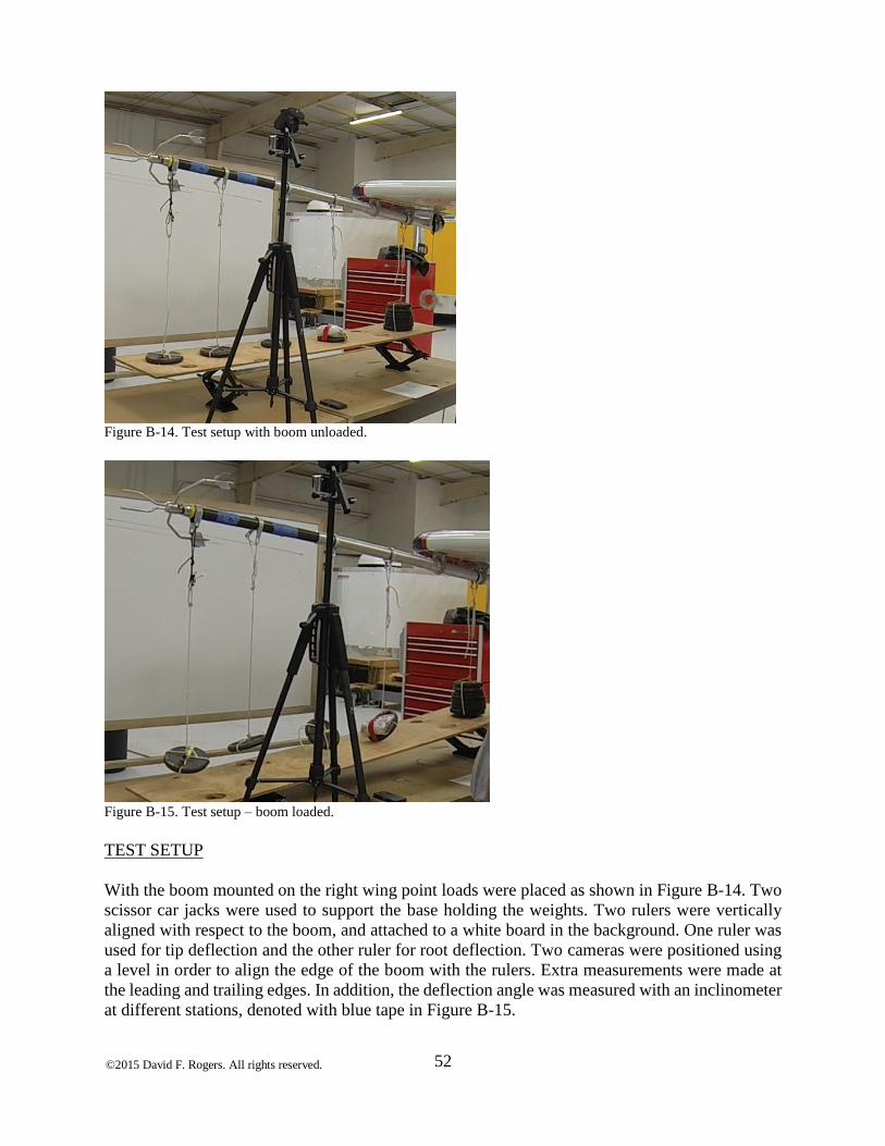
©2015 David F. Rogers. All rights reserved.
52
Figure B-14. Test setup with boom unloaded.
Figure B-15. Test setup – boom loaded.
TEST SETUP
With the boom mounted on the right wing point loads were placed as shown in Figure B-14. Two
scissor car jacks were used to support the base holding the weights. Two rulers were vertically
aligned with respect to the boom, and attached to a white board in the background. One ruler was
used for tip deflection and the other ruler for root deflection. Two cameras were positioned using
a level in order to align the edge of the boom with the rulers. Extra measurements were made at
the leading and trailing edges. In addition, the deflection angle was measured with an inclinometer
at different stations, denoted with blue tape in Figure B-15.
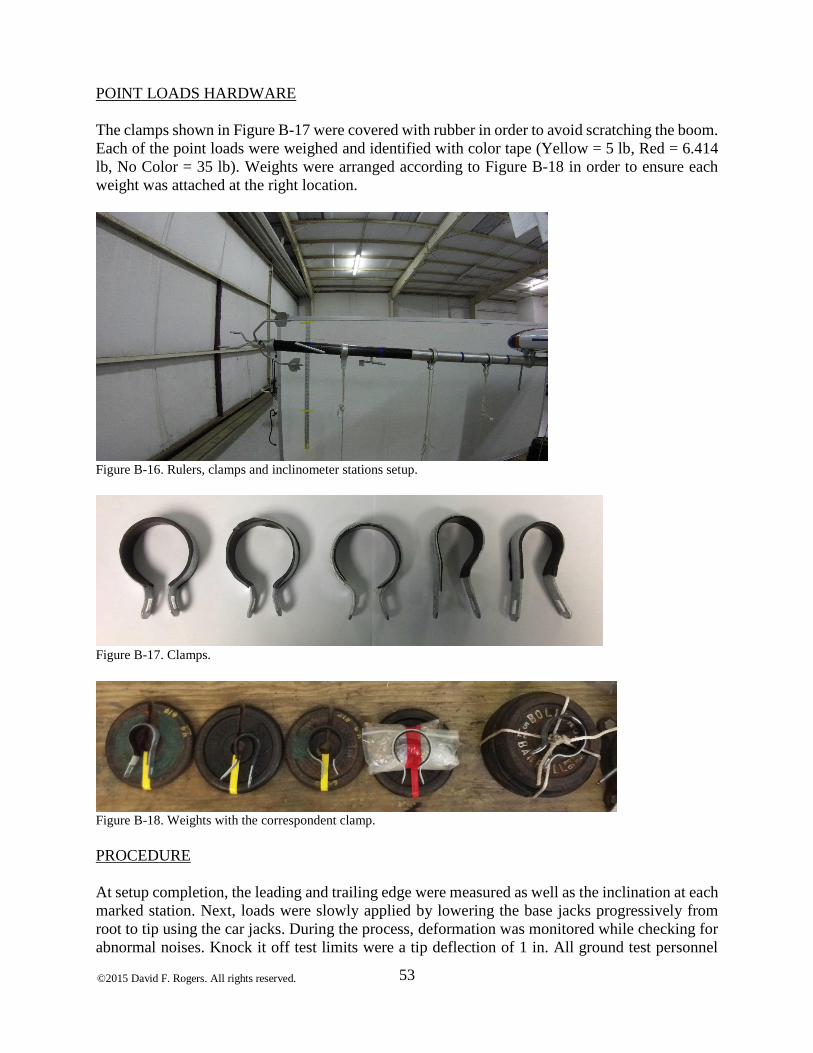
©2015 David F. Rogers. All rights reserved.
53
POINT LOADS HARDWARE
The clamps shown in Figure B-17 were covered with rubber in order to avoid scratching the boom.
Each of the point loads were weighed and identified with color tape (Yellow = 5 lb, Red = 6.414
lb, No Color = 35 lb). Weights were arranged according to Figure B-18 in order to ensure each
weight was attached at the right location.
Figure B-16. Rulers, clamps and inclinometer stations setup.
Figure B-17. Clamps.
Figure B-18. Weights with the correspondent clamp.
PROCEDURE
At setup completion, the leading and trailing edge were measured as well as the inclination at each
marked station. Next, loads were slowly applied by lowering the base jacks progressively from
root to tip using the car jacks. During the process, deformation was monitored while checking for
abnormal noises. Knock it off test limits were a tip deflection of 1 in. All ground test personnel

©2015 David F. Rogers. All rights reserved.
54
had knock it off authority. Once all weights cleared the base, the loading was maintained for one
minute. Measurements of deflection and displacement were taken again. The boom was then
unloaded, detached and inspected.
Table B-1. Deflection and displacement.
RESULTS
Table B-1 shows the results of the measurements before and after the one minute constant load.
The total deflection at the tip, using the superposition method, was 0.741 in, which approximates
the measurement from the ruler located at the tip as shown in Figure B-16. However, while the
boom was loaded, it experienced a rotation, which set the tip 0.203 in lower. In addition, the wing
experienced a displacement of 0.25 in, which resulted in 0.288 in of actual deflection at tip.
From the finite element analysis (FEA) the expected deflection was 0.219 in at the tip, which
represents a 31.5% calculation error. The limit for the test was set to 1 in deflection, leaving the
resulting value within the acceptable range. The difference between the actual load (available
hardware) and the true load varied from 1.5% to 29.4%. This results in a more conservative test
since in-flight loads are not expected to be greater than 4.4g.
As the boom was unloaded, the tip returned to its initial position. Finally, in the post-test inspection
all brackets, fasteners and rivets were checked, as well as the boom itself. There were no signs of
cracks, fatigue or deformation in any of the inspected elements.
Figure B-19. Boom – tip deflection.
Leading
Edge
Trailing
Edge
Unloaded 0.1 0.1 0.1 0.1 0.2 0.2 41 3/4 40
Loaded 0.1 0.2 0.4 0.5 0.8 0.8 41 1/2 39 3/4
Location (root to tip) [in] 8.38 22.3 37.38 49.8 66 76.8 83.00
Unloaded deflection 0.015 0.039 0.065 0.087 0.181 0.203
Loaded deflection 0.015 0.063 0.169 0.277 0.654 0.741
Rotation 0.000 0.024 0.103 0.190 0.473 0.538
Expected 0.219
%ERROR 31.50
Inclination [deg]
0.288
1/4 1/4
Experimental
©2015 David F. Rogers. All rights reserved.
55
DATA ACQUISITION AND INSTRUMENTATION
The aircraft’s data acquisition system (DAS) collects data from the Inertial Measurement Unit
(IMU), Global Position System (GPS) unit, total and static pressure transducers, and Angle of
Attack and Angle of Sideslip control position transducers. The IMU installed in the flight test
aircraft is the Honeywell HG1700. The IMU is able to record the aircraft’s velocity relative to the
ground, all pitch, roll, and yaw rates and angles, and also any accelerations acting on the aircraft.
For position reporting, the IMU communicates with the ProPak-V3 GPS unit, manufactured by
NovAtel.
The aircraft is equipped with a Precision Differential Pressure Transducer and Precision Static
Pressure Transducer (PPT’s) used to measure total pressure and static pressure, respectively. These
PPTs, manufactured by Honeywell, transform changes in pressure measured at the air data boom
into a digital signal that is recorded by the data acquisition system (DAS). Additionally, the air
data boom has an angle of attack vane and angle of sideslip vane that is attached to separate
potentiometers. These potentiometers, also known as Control Position Transducers (CPT’s), send
angle of sideslip and angle of attack measurements to the DAS via changes in signal voltage.
Similar to the PPT’s, the CPTs require calibration before they can be implemented.
Once these systems were installed on the aircraft, an initial ground calibration was completed. The
boom pitot and static ports were connected to a ground Pitot-Static tester and the system was tested
for airspeeds between 38 and 159 knots, and pressure altitudes between -100 and 9985 feet.
Furthermore, the angle of sideslip and angle of attack vanes were both tested between -90 and 90
degrees. The resulting conversion equations are given here for airspeed, pressure altitude, angle of
attack, and angle of sideslip, respectively. It is important to note that boom’s pitot-static system
was tested and verified to be leak free, and any inherent instrument error is negligible to the
subsequent analysis.
𝑉𝑖 = 206.28 × 𝑞𝑐𝑖0.5203
𝐻𝑖 = −2158.7 × 𝑃𝑠 + 31552
∝𝑖= −0.00281 × 𝑣∝ + 0.53235
𝛽𝑖 = −0.00295 × 𝑣𝛽 + 0.53892
The outside air temperature (OAT) and fuel quantities were manually entered into the DAS control
panel on the FTE’s laptop throughout flight. The fuel remaining quantities entered by the FTE
were obtained from a J.P. Instruments Fuel Scan 450 fuel monitoring system. The Fuel Scan 450,
which reports fuel flow, fuel used, and fuel remaining, is part of the extra instrumentation that was
installed previously on the aircraft. This system has been tested and calibrated through a functional
check flight prior to its use for subsequent flight testing. Lastly, the OAT was read directly off the
temperature gauge on the aircraft’s Aspen Evolution 1000 primary flight display.
The IMU, GPS, PPT, and CPT signals are interpreted by a National Instruments Compact
reconfigurable input/output (RIO) communications module. The Compact RIO simultaneously
logs this data in a raw format and outputs the data to a Flight Test Engineer’s laptop. The laptop
serves as both a master control module for the DAS system, as well as a data processing and
logging device. The laptop saves the processed data into a comma separated value file that is then
reduced and interpreted post-flight.
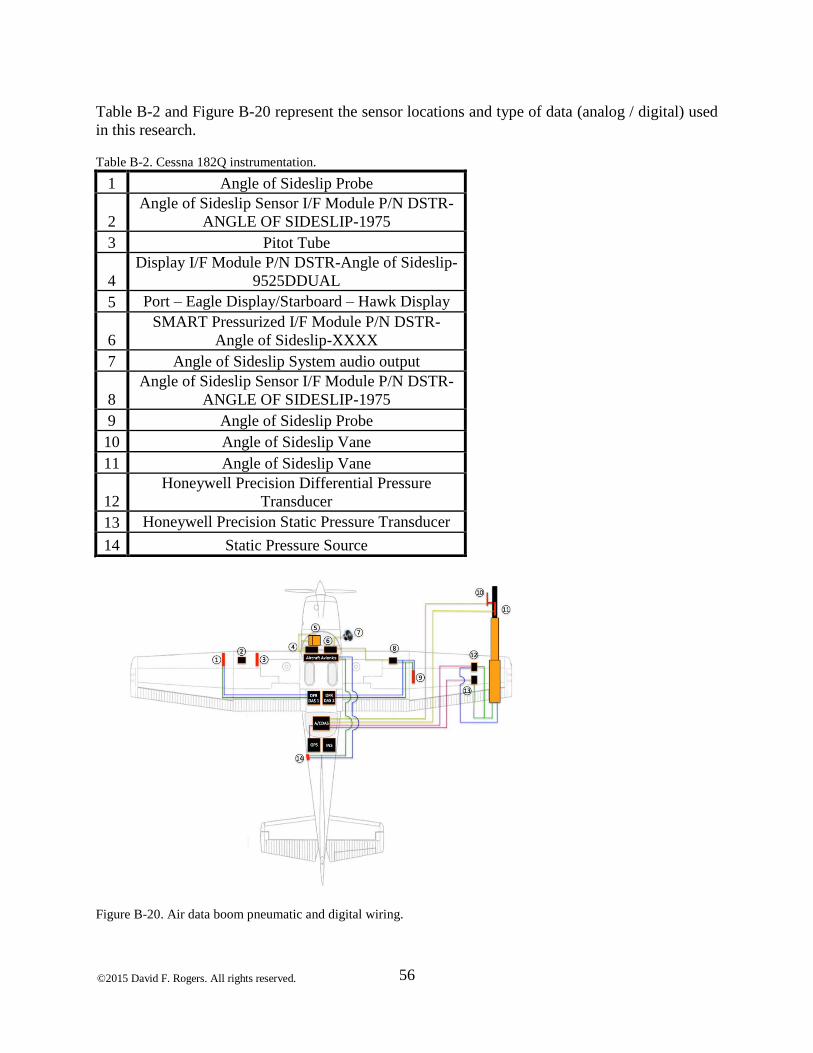
©2015 David F. Rogers. All rights reserved.
56
Table B-2 and Figure B-20 represent the sensor locations and type of data (analog / digital) used
in this research.
Table B-2. Cessna 182Q instrumentation.
1 Angle of Sideslip Probe
2
Angle of Sideslip Sensor I/F Module P/N DSTR-
ANGLE OF SIDESLIP-1975
3 Pitot Tube
4
Display I/F Module P/N DSTR-Angle of Sideslip-
9525DDUAL
5 Port – Eagle Display/Starboard – Hawk Display
6
SMART Pressurized I/F Module P/N DSTR-
Angle of Sideslip-XXXX
7 Angle of Sideslip System audio output
8
Angle of Sideslip Sensor I/F Module P/N DSTR-
ANGLE OF SIDESLIP-1975
9 Angle of Sideslip Probe
10 Angle of Sideslip Vane
11 Angle of Sideslip Vane
12
Honeywell Precision Differential Pressure
Transducer
13 Honeywell Precision Static Pressure Transducer
14 Static Pressure Source
Figure B-20. Air data boom pneumatic and digital wiring.
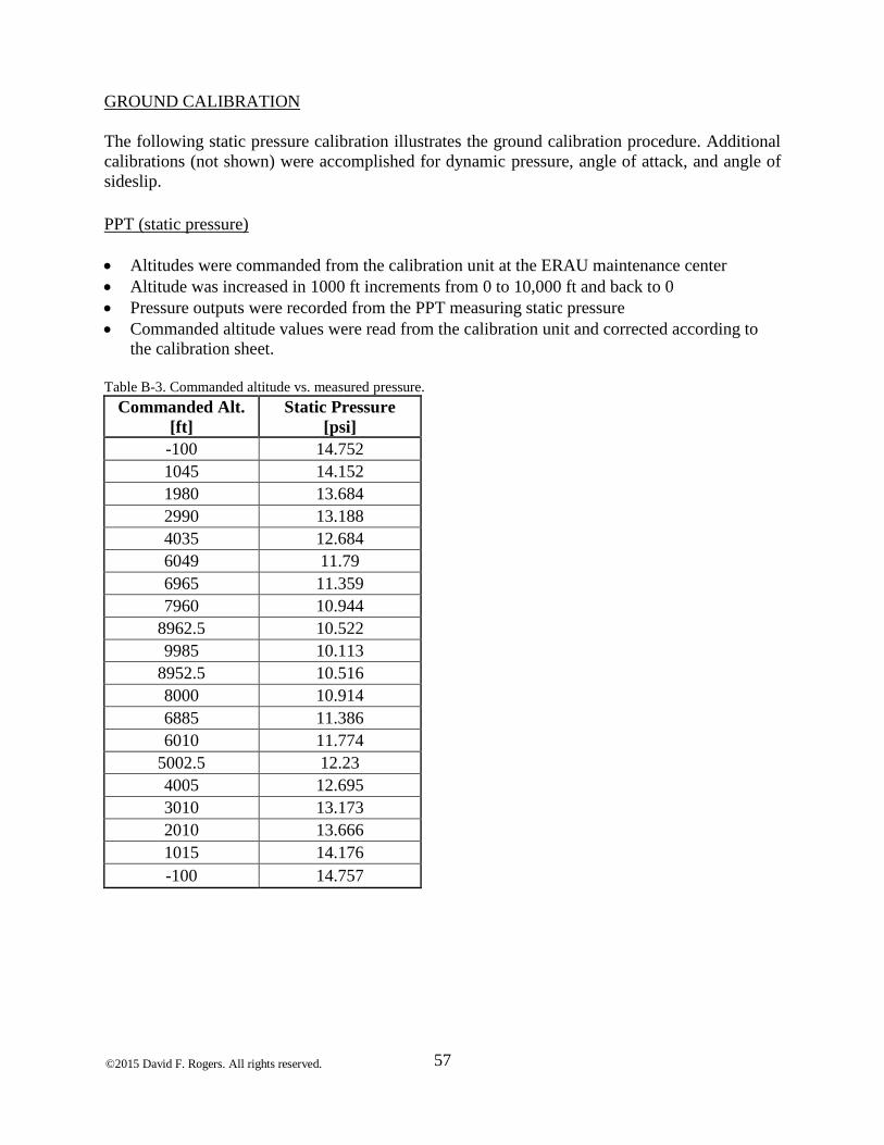
©2015 David F. Rogers. All rights reserved.
57
GROUND CALIBRATION
The following static pressure calibration illustrates the ground calibration procedure. Additional
calibrations (not shown) were accomplished for dynamic pressure, angle of attack, and angle of
sideslip.
PPT (static pressure)
Altitudes were commanded from the calibration unit at the ERAU maintenance center
Altitude was increased in 1000 ft increments from 0 to 10,000 ft and back to 0
Pressure outputs were recorded from the PPT measuring static pressure
Commanded altitude values were read from the calibration unit and corrected according to
the calibration sheet.
Table B-3. Commanded altitude vs. measured pressure.
Commanded Alt.
[ft]
Static Pressure
[psi]
-100 14.752
1045 14.152
1980 13.684
2990 13.188
4035 12.684
6049 11.79
6965 11.359
7960 10.944
8962.5 10.522
9985 10.113
8952.5 10.516
8000 10.914
6885 11.386
6010 11.774
5002.5 12.23
4005 12.695
3010 13.173
2010 13.666
1015 14.176
-100 14.757
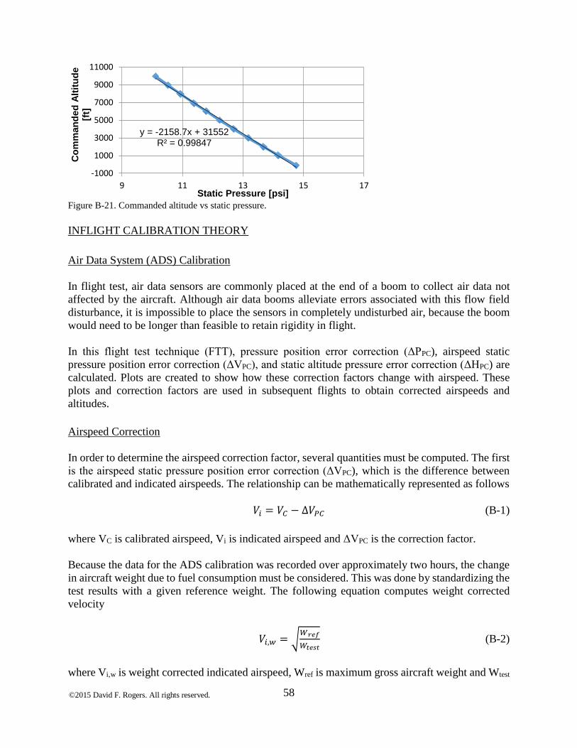
©2015 David F. Rogers. All rights reserved.
58
Figure B-21. Commanded altitude vs static pressure.
INFLIGHT CALIBRATION THEORY
Air Data System (ADS) Calibration
In flight test, air data sensors are commonly placed at the end of a boom to collect air data not
affected by the aircraft. Although air data booms alleviate errors associated with this flow field
disturbance, it is impossible to place the sensors in completely undisturbed air, because the boom
would need to be longer than feasible to retain rigidity in flight.
In this flight test technique (FTT), pressure position error correction (ΔPPC), airspeed static
pressure position error correction (ΔVPC), and static altitude pressure error correction (ΔHPC) are
calculated. Plots are created to show how these correction factors change with airspeed. These
plots and correction factors are used in subsequent flights to obtain corrected airspeeds and
altitudes.
Airspeed Correction
In order to determine the airspeed correction factor, several quantities must be computed. The first
is the airspeed static pressure position error correction (ΔVPC), which is the difference between
calibrated and indicated airspeeds. The relationship can be mathematically represented as follows
𝑉𝑖 = 𝑉𝐶 − Δ𝑉𝑃𝐶 (B-1)
where VC is calibrated airspeed, Vi is indicated airspeed and ΔVPC is the correction factor.
Because the data for the ADS calibration was recorded over approximately two hours, the change
in aircraft weight due to fuel consumption must be considered. This was done by standardizing the
test results with a given reference weight. The following equation computes weight corrected
velocity
𝑉𝑖,𝑤 = √𝑊𝑟𝑒𝑓
𝑊𝑡𝑒𝑠𝑡 (B-2)
where Vi,w is weight corrected indicated airspeed, Wref is maximum gross aircraft weight and Wtest
y = -2158.7x + 31552R² = 0.99847
-1000
1000
3000
5000
7000
9000
11000
9 11 13 15 17
Co
mm
an
ded
Alt
itu
de
[ft]
Static Pressure [psi]

©2015 David F. Rogers. All rights reserved.
59
is gross aircraft weight less fuel used.
At Mach numbers below 0.3 compressibility effects can be ignored. Under these conditions, true
airspeed and equivalent airspeed (VE) are assumed equal. The relationship between equivalent and
true airspeed is
𝑉𝐸 = √𝜎 ∙ 𝑉𝑇 (B-3)
where VT is true airspeed and σ is density ratio
Position Correction
The second correction factor is the static pressure position error coefficient. This correction
nondimensionalizes the data in order to compare and graph the results of the ADS Calibration. The
measured dynamic pressure is
𝑞𝐶𝑖 = 𝑃𝑆𝑆𝐿 ((𝜌𝑆𝑆𝐿∙𝑉𝑖,𝑤
2
(𝑃𝑆𝑆𝐿 ∙7)+1)
𝛾𝛾−1⁄
− 1) (B-4)
where qCi is the measured dynamic pressure.
The static pressure position coefficient is calculated by taking the difference between the two
dynamic pressures
Δ𝑃𝑃𝐶 = 𝑞𝐶 − 𝑞𝐶𝑖 (B-5)
Altitude Correction
The last correction factor is the altitude static position error (ΔHPC) which accounts for the
altimeter static pressure error. This factor is computed using the hydrostatic equation:
Δ𝐻𝑃𝐶 =Δ𝑃𝑃𝐶
𝜌𝑔 (B-6)
Upwash Calibration
Upwash calibration is used to determine errors in the indicated angle of attack that result from
upwash in the flow field. Upwash decreases ahead of the wing leading edge and, theoretically, if
placed far enough forward, upwash is negligible. Theory suggests that this distance is at least 1.5
fuselage diameters ahead of the wing. Completely removing any upwash sensed by the boom
would require an unfeasibly long boom. The upwash correction removes this error and obtains the
true angle of attack, measured with respect to the fuselage reference line (FRL) in-flight.
Because of the way the data acquisition system (DAS) sensors are installed, other measurement
errors need to be accounted for. After reducing data, a correction factor is then determined to
calculate the true angle of attack, which is then compared to other angle of attack instruments to
©2015 David F. Rogers. All rights reserved.
60
determine its accuracy.
A direct way of calculating upwash is to compare the indicated angle of attack to the true angle of
attack, given by
∆𝛼 = |𝛼𝑇 − 𝛼𝑖| (B-7)
where 𝛼𝑡𝑟𝑢𝑒 is
𝛼𝑡𝑟𝑢𝑒 = 𝜃 − 𝛾 (B-8)
where 𝜃 is pitch attitude and 𝛾 is flight path angle. The flight path angle can be determined from
𝛾 = sin−1 (𝑑ℎ
𝑑𝑡
𝑉𝑇) (B-9)
During straight and level un-accelerated flight, 𝛾 is zero. This justifies the assumption that angle
of attack is equal to pitch angle in straight and level un-accelerated flight. The upwash angle is
calculated from
∆𝛼 = sin−1(𝑛𝑥𝑎𝑐𝑐𝑒𝑙 − 𝑛𝑥𝑝𝑟𝑒𝑠𝑠) (B-10)
where 𝑛𝑥𝑎𝑐𝑐𝑒𝑙 and 𝑛𝑥𝑝𝑟𝑒𝑠𝑠 are defined respectively as
𝑛𝑥𝑎𝑐𝑐𝑒𝑙 = 𝑛𝑥𝑏𝑐𝑜𝑠𝛼𝑖 − 𝑛𝑧𝑏𝑠𝑖𝑛𝛼𝑖 (B-11)
𝑛𝑥𝑝𝑟𝑒𝑠𝑠 =ℎ̇
𝑉𝑇+
𝑉�̇�
𝑔 (B-12)
where 𝑛𝑥𝑏 is instrumented body-axis longitudinal load factor, 𝑛𝑧𝑏 is instrumented body-axis
vertical load factor, ℎ̇ is geometric climb rate from pressure altitude corrected for test day
temperature, 𝑉𝑇 is true airspeed, 𝑉�̇� is rate of change of true airspeed, g is gravitational acceleration
constant, 𝛼𝑖 is indicated angle of attack and 𝑛𝑥𝑝𝑟𝑒𝑠𝑠 is used to correct for small vertical velocities
or accelerations that are present during steady state trim shots.

©2015 David F. Rogers. All rights reserved.
61
IN-FLIGHT CALIBRATION RESULTS
ADS Calibration
Table B-4. Velocity corrections as listed in the pilot’s operating handbook (POH).
Table B-4 contains the POH velocity static pressure position corrections along with the reported
indicated airspeed corrections. The aircraft calibrated airspeed was calculated using the airspeeds
in the reduction algorithm. For a graphical representation of these correction factors, refer to Figure
B-22.
Table B-5 contains correction factors calculated using an ADS calibration reduction algorithm.
These values were then used throughout the rest of the algorithm including upwash calibration and
stall testing plots. Individual equations and graphical representations are included in Figures B-23,
B-24 and B-25.
Figure B-22 represents the accuracy of the calculated correction factors. Various horizontal and
vertical lines are used to show that both pitot and ERAU DAS indicated airspeeds (when corrected)
provide the same calibrated airspeeds. These values fell within +/- 0.5 knots of each other. Figure
B-23 shows the results of the ADS calibration on the trimmed DAS data.
Airspeed
KIAS 50 60 70 80 90 100 110 120 130 140 150 160
KCAS 60 64 71 80 89 99 108 117 127 136 145 155
Aircraft
Calculated
KCAS
55.4 63.7 72.2 80.7 89.2 97.8 106.5 115.2 124.0 132.9 141.8 150.7
% Error 7.7% 0.4% 1.6% 0.8% 0.2% 1.2% 1.4% 1.5% 2.4% 2.3% 2.2% 2.7%
POH Values
Viw_DAS PEC_DAS dVpc_DAS dHpc_DAS
KIAS Unitless Knots Feet
119.48 0.06 3.48 41.66
93.17 0.10 4.51 42.50
79.39 0.11 4.22 33.77
71.20 0.10 3.46 24.68
65.48 0.11 3.40 22.34
61.09 0.13 3.95 24.38
59.05 0.10 2.82 16.64
Table B-5. Correction values determined during ADS calibration.
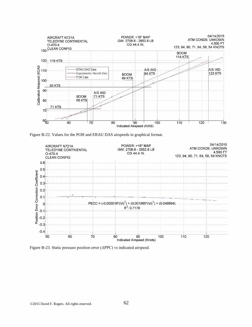
©2015 David F. Rogers. All rights reserved.
62
Figure B-22. Values for the POH and ERAU DAS airspeeds in graphical format.
Figure B-23. Static pressure position error (ΔPPC) vs indicated airspeed.
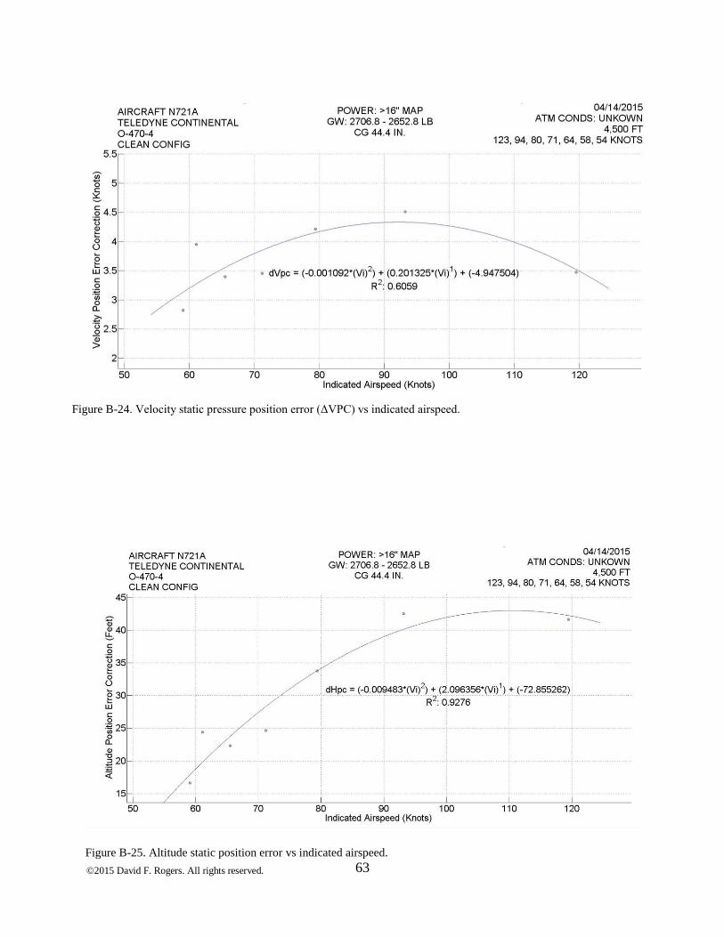
©2015 David F. Rogers. All rights reserved.
63
Figure B-24. Velocity static pressure position error (ΔVPC) vs indicated airspeed.
Figure B-25. Altitude static position error vs indicated airspeed.
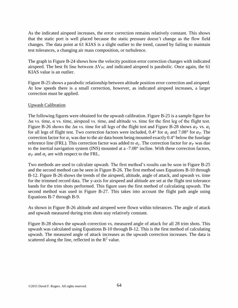
©2015 David F. Rogers. All rights reserved.
64
As the indicated airspeed increases, the error correction remains relatively constant. This shows
that the static port is well placed because the static pressure doesn’t change as the flow field
changes. The data point at 61 KIAS is a slight outlier to the trend, caused by failing to maintain
test tolerances, a changing air mass composition, or turbulence.
The graph in Figure B-24 shows how the velocity position error correction changes with indicated
airspeed. The best fit line between ΔVPC and indicated airspeed is parabolic. Once again, the 61
KIAS value is an outlier.
Figure B-25 shows a parabolic relationship between altitude position error correction and airspeed.
At low speeds there is a small correction, however, as indicated airspeed increases, a larger
correction must be applied.
Upwash Calibration
The following figures were obtained for the upwash calibration. Figure B-25 is a sample figure for
Δα vs. time, α vs. time, airspeed vs. time, and altitude vs. time for the first leg of the flight test.
Figure B-26 shows the Δα vs. time for all legs of the flight test and Figure B-28 shows 𝛼𝑇 vs. 𝛼𝑖 for all legs of flight test. Two correction factors were included, 0.4° for 𝛼𝑖 and 7.08° for 𝛼𝑇 . The
correction factor for 𝛼𝑖 was due to the air data boom being mounted exactly 0.4° below the fuselage
reference line (FRL). This correction factor was added to 𝛼𝑖. The correction factor for 𝛼𝑇 was due
to the inertial navigation system (INS) mounted at a -7.08° incline. With these correction factors,
𝛼𝑇 and 𝛼𝑖 are with respect to the FRL.
Two methods are used to calculate upwash. The first method’s results can be seen in Figure B-25
and the second method can be seen in Figure B-26. The first method uses Equations B-10 through
B-12. Figure B-26 shows the trends of the airspeed, altitude, angle of attack, and upwash vs. time
for the trimmed record data. The y-axis for airspeed and altitude are set at the flight test tolerance
bands for the trim shots performed. This figure uses the first method of calculating upwash. The
second method was used in Figure B-27. This takes into account the flight path angle using
Equations B-7 through B-9.
As shown in Figure B-26 altitude and airspeed were flown within tolerances. The angle of attack
and upwash measured during trim shots stay relatively constant.
Figure B-28 shows the upwash correction vs. measured angle of attack for all 28 trim shots. This
upwash was calculated using Equations B-10 through B-12. This is the first method of calculating
upwash. The measured angle of attack increases as the upwash correction increases. The data is
scattered along the line, reflected in the R2 value.
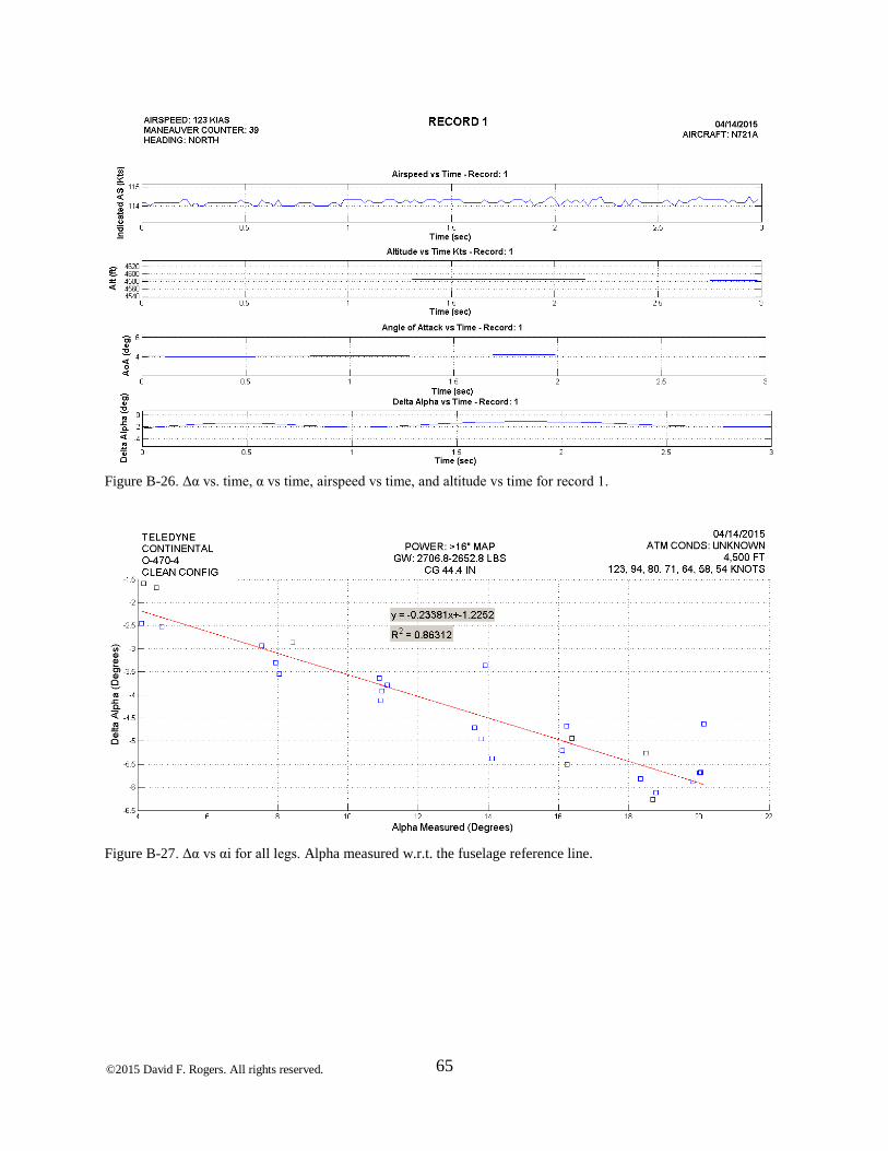
©2015 David F. Rogers. All rights reserved.
65
Figure B-26. Δα vs. time, α vs time, airspeed vs time, and altitude vs time for record 1.
Figure B-27. Δα vs αi for all legs. Alpha measured w.r.t. the fuselage reference line.
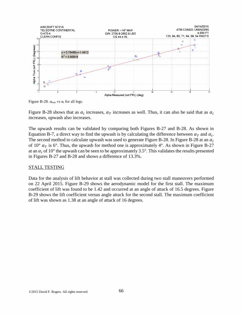
©2015 David F. Rogers. All rights reserved.
66
Figure B-28. αtrue vs αi for all legs.
Figure B-28 shows that as 𝛼𝑖 increases, 𝛼𝑇 increases as well. Thus, it can also be said that as 𝛼𝑖
increases, upwash also increases.
The upwash results can be validated by comparing both Figures B-27 and B-28. As shown in
Equation B-7, a direct way to find the upwash is by calculating the difference between 𝛼𝑇 and 𝛼𝑖.
The second method to calculate upwash was used to generate Figure B-28. In Figure B-28 at an 𝛼𝑖
of 10° 𝛼𝑇 is 6°. Thus, the upwash for method one is approximately 4°. As shown in Figure B-27
at an 𝛼𝑖 of 10° the upwash can be seen to be approximately 3.5°. This validates the results presented
in Figures B-27 and B-28 and shows a difference of 13.3%.
STALL TESTING
Data for the analysis of lift behavior at stall was collected during two stall maneuvers performed
on 22 April 2015. Figure B-29 shows the aerodynamic model for the first stall. The maximum
coefficient of lift was found to be 1.42 and occurred at an angle of attack of 16.5 degrees. Figure
B-29 shows the lift coefficient versus angle attack for the second stall. The maximum coefficient
of lift was shown as 1.38 at an angle of attack of 16 degrees.
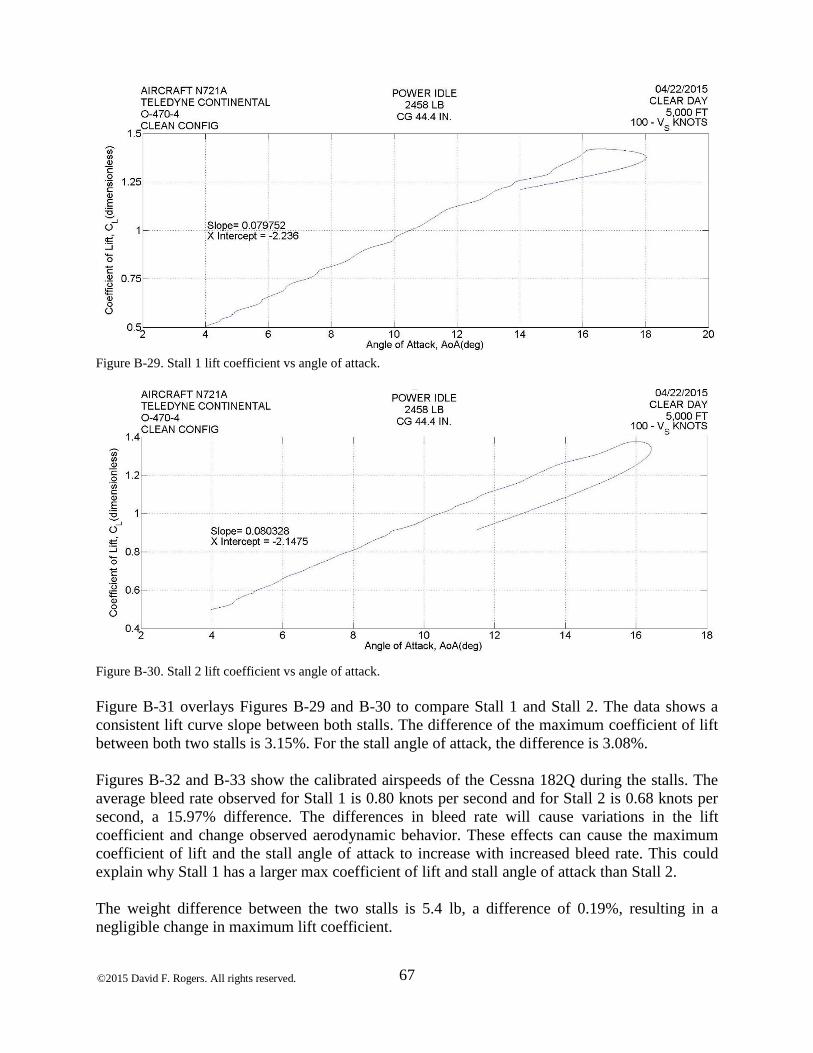
©2015 David F. Rogers. All rights reserved.
67
Figure B-29. Stall 1 lift coefficient vs angle of attack.
Figure B-30. Stall 2 lift coefficient vs angle of attack.
Figure B-31 overlays Figures B-29 and B-30 to compare Stall 1 and Stall 2. The data shows a
consistent lift curve slope between both stalls. The difference of the maximum coefficient of lift
between both two stalls is 3.15%. For the stall angle of attack, the difference is 3.08%.
Figures B-32 and B-33 show the calibrated airspeeds of the Cessna 182Q during the stalls. The
average bleed rate observed for Stall 1 is 0.80 knots per second and for Stall 2 is 0.68 knots per
second, a 15.97% difference. The differences in bleed rate will cause variations in the lift
coefficient and change observed aerodynamic behavior. These effects can cause the maximum
coefficient of lift and the stall angle of attack to increase with increased bleed rate. This could
explain why Stall 1 has a larger max coefficient of lift and stall angle of attack than Stall 2.
The weight difference between the two stalls is 5.4 lb, a difference of 0.19%, resulting in a
negligible change in maximum lift coefficient.
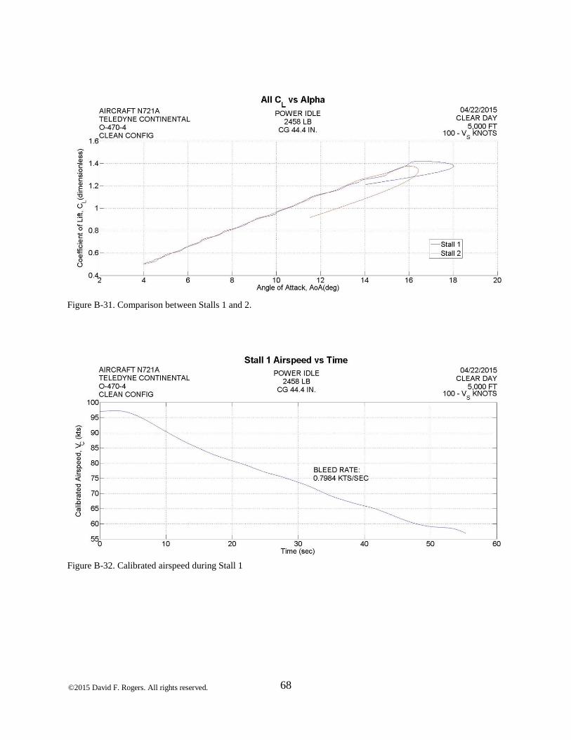
©2015 David F. Rogers. All rights reserved.
68
Figure B-31. Comparison between Stalls 1 and 2.
Figure B-32. Calibrated airspeed during Stall 1
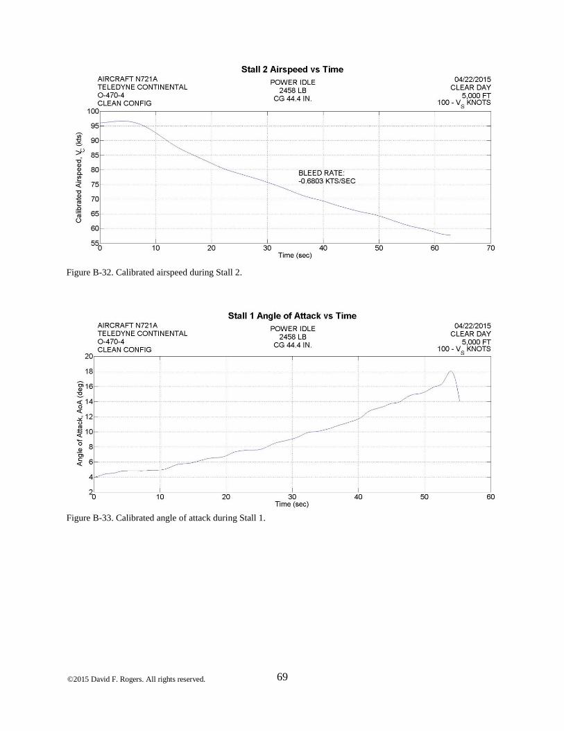
©2015 David F. Rogers. All rights reserved.
69
Figure B-32. Calibrated airspeed during Stall 2.
Figure B-33. Calibrated angle of attack during Stall 1.

©2015 David F. Rogers. All rights reserved.
70
Figure B-34. Calibrated angle of attack during Stall 2.
The theoretical value for the lift curve slope of the Cessna 182Q was estimated at 0.08 per degree.
Comparing this theoretical value to each individual stall, Stall 1 showed a difference of 0.057%
and 0.41% difference for Stall 2. The average of the data was 0.0800 per degree, which has zero
difference. Significant figures failed to capture the exact difference. The NACA 2412 airfoil in
this aircraft has a maximum coefficient of lift of 1.5 to 1.7 at a geometric angle of attack of about
16 degrees depending on aerodynamic center location and atmospheric conditions. With the
assumption that 90% of the airfoil max lift coefficient can estimate the theoretical max lift
coefficient the aircraft, the Cessna 182Q should have a theoretical value of 1.44 for the max lift
coefficient. The average max coefficient of lift value was 1.40, a 2.86% difference from the
theoretical value. The average geometric stall angle of attack was 16.25 degrees, differing by
1.55% from the airfoil’s theoretical value.
The calibration methods showed a parabolic relationship for dVpc and dHpc while the PEC
remained fairly constant. The dVpc correction factor peaks at 94 KIAS at an approximate value of
4.5 knots. Compared to the POH data, the velocity pressure position corrections at each indicated
airspeed show a largest error of 7.7%. The dHpc correction factor peaks at approximately 110 KIAS
with an approximate value of 43 feet. Furthermore, the results of the upwash calibration
determined that as the angle of attack increases, the upwash correction also increased. A validation
of these results was done by using two different methods to reach the same conclusion, showing a
13.3% difference in Δα at an α of 10 degrees. The last flight test technique showed that the
maximum lift coefficient and stall angle of attack had errors of 5.71% and 12.1% respectively.

71 ©2015 David F. Rogers. All rights reserved.
APPENDIX C. AERODYNAMICS OF WHY A LINEAR CALIBRATION WORKS
Six frame grabs from a 1938 NACA film [NACA38] are shown in Figure C-1 (two of these frame
grabs, (a) and (f), are also shown in Figure 30). These images illustrate the underlying principle
that results in a linear calibration curve for under wing mounted differential angle of attack probes.
The airfoil in the frame grabs is a symmetrical airfoil.
The pressure on the surface of the airfoil referenced to the free stream (atmospheric) pressure is
positive in the vicinity of the stagnation point but generally negative on the upper surface and may
be negative or positive on the lower surface (see Figure C-2 or 31). Generally, other than near the
stagnation point, if the pressure relative to the atmosphere pressure is positive on the lower surface
it is positive at low angles of attack near the trailing edge or when flaps are deployed.
Figure C-1. Frame grabs showing the streamlines around an airfoil without flaps extended.
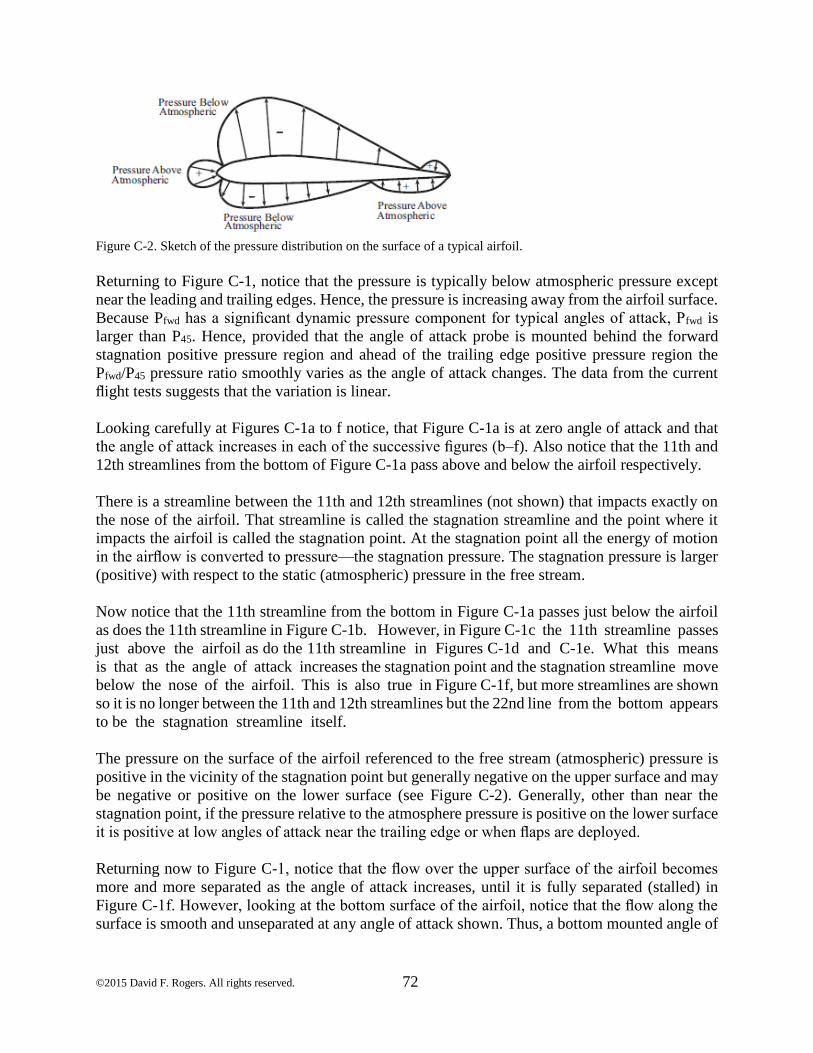
72 ©2015 David F. Rogers. All rights reserved.
Figure C-2. Sketch of the pressure distribution on the surface of a typical airfoil.
Returning to Figure C-1, notice that the pressure is typically below atmospheric pressure except
near the leading and trailing edges. Hence, the pressure is increasing away from the airfoil surface.
Because Pfwd has a significant dynamic pressure component for typical angles of attack, Pfwd is
larger than P45. Hence, provided that the angle of attack probe is mounted behind the forward
stagnation positive pressure region and ahead of the trailing edge positive pressure region the
Pfwd/P45 pressure ratio smoothly varies as the angle of attack changes. The data from the current
flight tests suggests that the variation is linear.
Looking carefully at Figures C-1a to f notice, that Figure C-1a is at zero angle of attack and that
the angle of attack increases in each of the successive figures (b–f). Also notice that the 11th and
12th streamlines from the bottom of Figure C-1a pass above and below the airfoil respectively.
There is a streamline between the 11th and 12th streamlines (not shown) that impacts exactly on
the nose of the airfoil. That streamline is called the stagnation streamline and the point where it
impacts the airfoil is called the stagnation point. At the stagnation point all the energy of motion
in the airflow is converted to pressure—the stagnation pressure. The stagnation pressure is larger
(positive) with respect to the static (atmospheric) pressure in the free stream.
Now notice that the 11th streamline from the bottom in Figure C-1a passes just below the airfoil
as does the 11th streamline in Figure C-1b. However, in Figure C-1c the 11th streamline passes
just above the airfoil as do the 11th streamline in Figures C-1d and C-1e. What this means
is that as the angle of attack increases the stagnation point and the stagnation streamline move
below the nose of the airfoil. This is also true in Figure C-1f, but more streamlines are shown
so it is no longer between the 11th and 12th streamlines but the 22nd line from the bottom appears
to be the stagnation streamline itself.
The pressure on the surface of the airfoil referenced to the free stream (atmospheric) pressure is
positive in the vicinity of the stagnation point but generally negative on the upper surface and may
be negative or positive on the lower surface (see Figure C-2). Generally, other than near the
stagnation point, if the pressure relative to the atmosphere pressure is positive on the lower surface
it is positive at low angles of attack near the trailing edge or when flaps are deployed.
Returning now to Figure C-1, notice that the flow over the upper surface of the airfoil becomes
more and more separated as the angle of attack increases, until it is fully separated (stalled) in
Figure C-1f. However, looking at the bottom surface of the airfoil, notice that the flow along the
surface is smooth and unseparated at any angle of attack shown. Thus, a bottom mounted angle of

73 ©2015 David F. Rogers. All rights reserved.
attack probe is operating in a smoothly varying pressure field. The pressure far away from the
airfoil surface must return to freestream (atmospheric) pressure.
Figure C-3 shows several frame grabs from the video [NACA38] for the same airfoil with a flap
deployed. Again, the streamlines on the lower surface are smooth and remain smooth with
increasing angle of attack. Hence, the pressure field on the bottom of the airfoil is also smooth.
Thus, the angle of attack probe behaves in a similar manner as without a flap deployed.
Figure C-3. Frame grabs showing the streamlines around an airfoil with flaps extended.
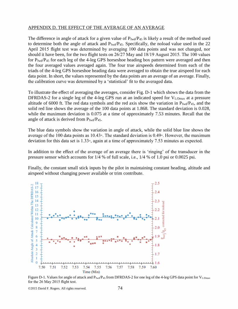
74 ©2015 David F. Rogers. All rights reserved.
APPENDIX D. THE EFFECT OF THE AVERAGE OF AN AVERAGE
The difference in angle of attack for a given value of Pfwd/P45 is likely a result of the method used
to determine both the angle of attack and Pfwd/P45. Specifically, the noload value used in the 22
April 2015 flight test was determined by averaging 100 data points and was not changed, nor
should it have been, for the two flight tests on 26/27 May and 18/19 August 2015. The 100 values
for Pfwd/P45 for each leg of the 4-leg GPS horseshoe heading box pattern were averaged and then
the four averaged values averaged again. The four true airspeeds determined from each of the
triads of the 4-leg GPS horseshoe heading data were averaged to obtain the true airspeed for each
data point. In short, the values represented by the data points are an average of an average. Finally,
the calibration curve was determined by a ‘statistical’ fit to the averaged data.
To illustrate the effect of averaging the averages, consider Fig. D-1 which shows the data from the
DFRDAS-2 for a single leg of the 4-leg GPS run at an indicated speed for VL/Dmax at a pressure
altitude of 6000 ft. The red data symbols and the red axis show the variation in Pfwd/P45, and the
solid red line shows the average of the 100 data points at 1.868. The standard deviation is 0.028,
while the maximum deviation is 0.075 at a time of approximately 7.53 minutes. Recall that the
angle of attack is derived from Pfwd/P45.
The blue data symbols show the variation in angle of attack, while the solid blue line shows the
average of the 100 data points as 10.43◦. The standard deviation is 0.49◦. However, the maximum
deviation for this data set is 1.33◦, again at a time of approximately 7.53 minutes as expected.
In addition to the effect of the average of an average there is ‘ringing’ of the transducer in the
pressure sensor which accounts for 1/4 % of full scale, i.e., 1/4 % of 1.0 psi or 0.0025 psi.
Finally, the constant small stick inputs by the pilot in maintaining constant heading, altitude and
airspeed without changing power available or trim contribute.
Figure D-1. Values for angle of attack and Pfwd/P45 from DFRDAS-2 for one leg of the 4-leg GPS data point for VL/Dmax
for the 26 May 2015 flight test.
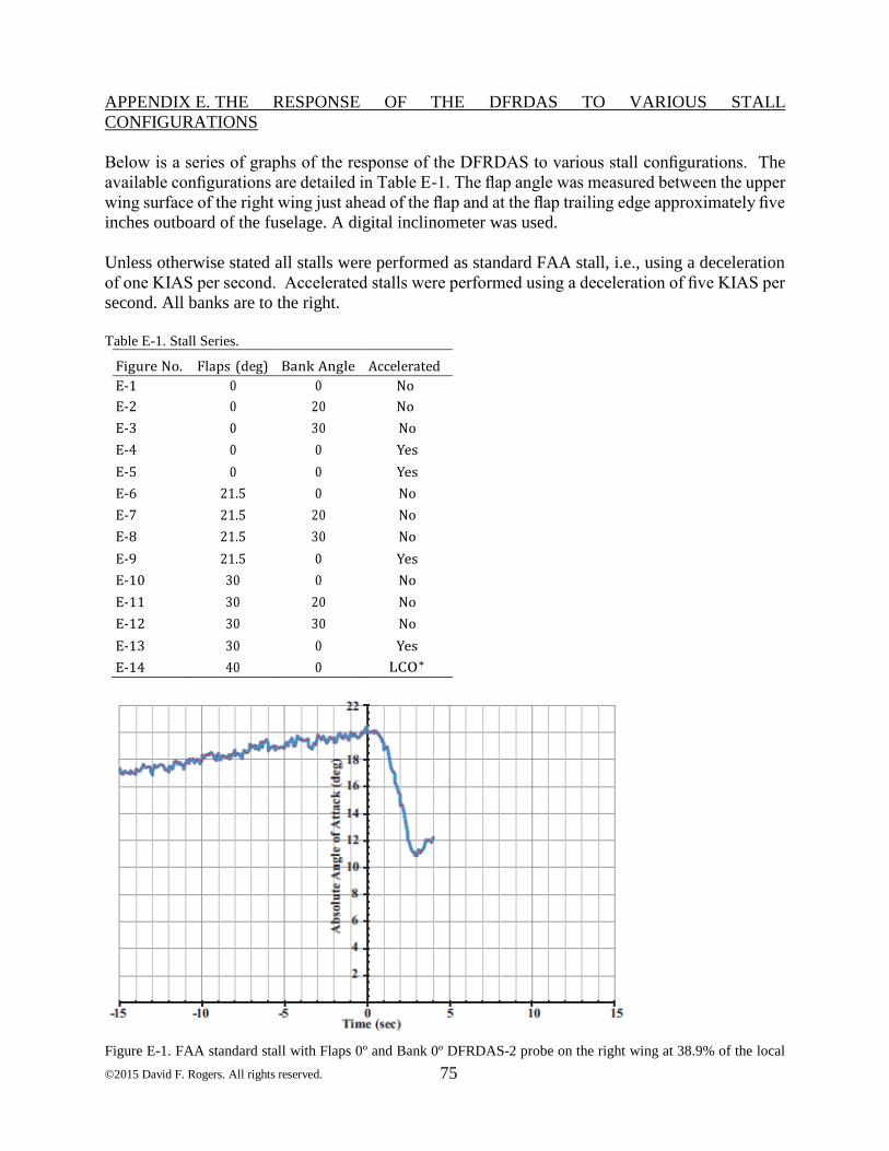
75 ©2015 David F. Rogers. All rights reserved.
APPENDIX E. THE RESPONSE OF THE DFRDAS TO VARIOUS STALL
CONFIGURATIONS
Below is a series of graphs of the response of the DFRDAS to various stall configurations. The
available configurations are detailed in Table E-1. The flap angle was measured between the upper
wing surface of the right wing just ahead of the flap and at the flap trailing edge approximately five
inches outboard of the fuselage. A digital inclinometer was used.
Unless otherwise stated all stalls were performed as standard FAA stall, i.e., using a deceleration
of one KIAS per second. Accelerated stalls were performed using a deceleration of five KIAS per
second. All banks are to the right.
Table E-1. Stall Series.
Figure No. Flaps (deg) Bank Angle Accelerated
E-1 0 0 No
E-2 0 20 No
E-3 0 30 No
E-4 0 0 Yes
E-5 0 0 Yes
E-6 21.5 0 No
E-7 21.5 20 No
E-8 21.5 30 No
E-9 21.5 0 Yes
E-10 30 0 No
E-11 30 20 No
E-12 30 30 No
E-13 30 0 Yes
E-14 40 0 LCO∗
Figure E-1. FAA standard stall with Flaps 0º and Bank 0º DFRDAS-2 probe on the right wing at 38.9% of the local
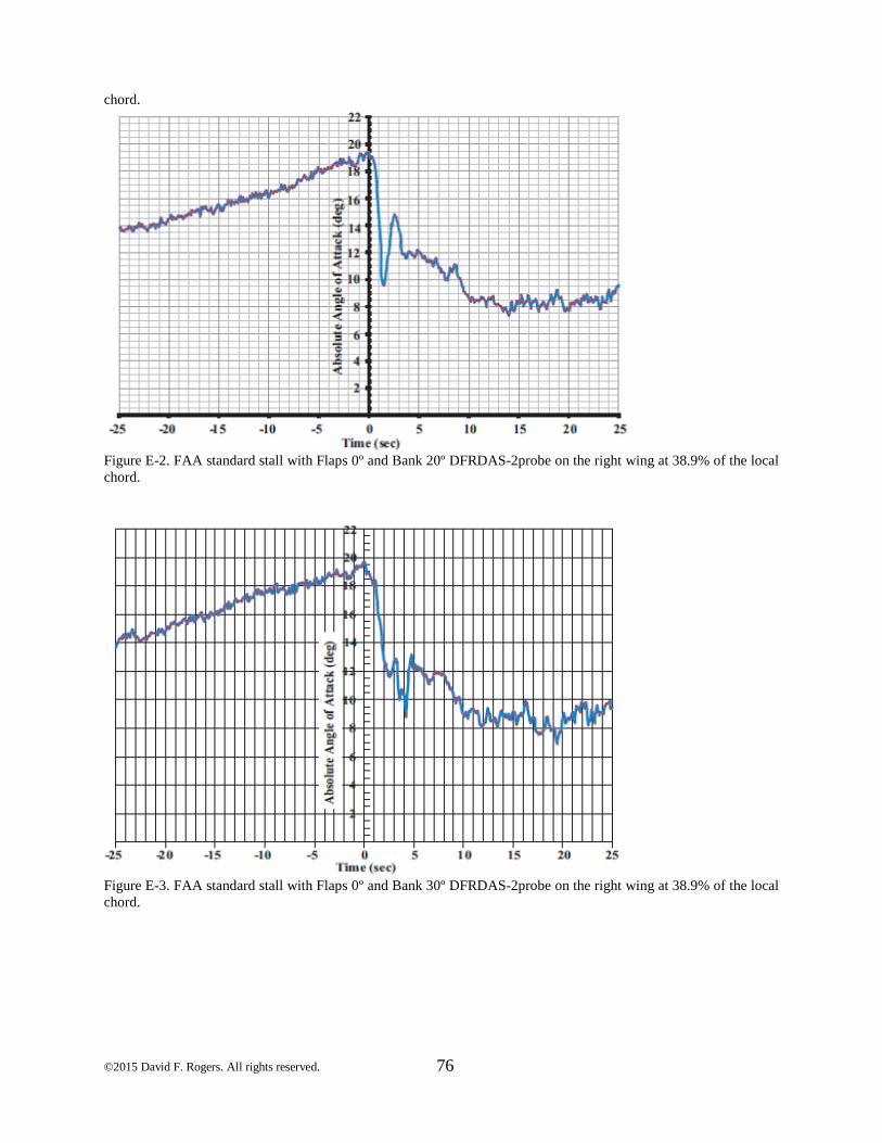
76 ©2015 David F. Rogers. All rights reserved.
chord.
Figure E-2. FAA standard stall with Flaps 0º and Bank 20º DFRDAS-2probe on the right wing at 38.9% of the local
chord.
Figure E-3. FAA standard stall with Flaps 0º and Bank 30º DFRDAS-2probe on the right wing at 38.9% of the local
chord.
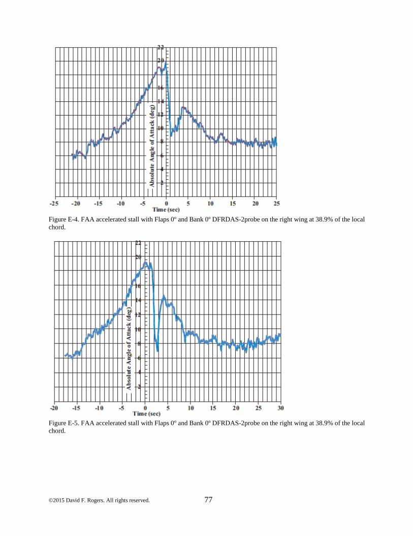
77 ©2015 David F. Rogers. All rights reserved.
Figure E-4. FAA accelerated stall with Flaps 0º and Bank 0º DFRDAS-2probe on the right wing at 38.9% of the local
chord.
Figure E-5. FAA accelerated stall with Flaps 0º and Bank 0º DFRDAS-2probe on the right wing at 38.9% of the local
chord.
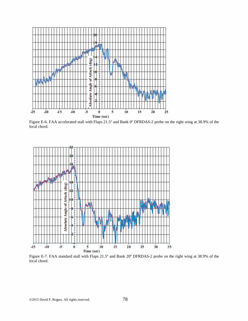
78 ©2015 David F. Rogers. All rights reserved.
Figure E-6. FAA accelerated stall with Flaps 21.5º and Bank 0º DFRDAS-2 probe on the right wing at 38.9% of the
local chord.
Figure E-7. FAA standard stall with Flaps 21.5º and Bank 20º DFRDAS-2 probe on the right wing at 38.9% of the
local chord.
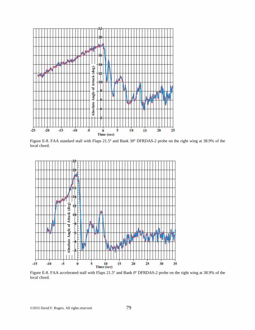
79 ©2015 David F. Rogers. All rights reserved.
Figure E-8. FAA standard stall with Flaps 21.5º and Bank 30º DFRDAS-2 probe on the right wing at 38.9% of the
local chord.
Figure E-8. FAA accelerated stall with Flaps 21.5º and Bank 0º DFRDAS-2 probe on the right wing at 38.9% of the
local chord.
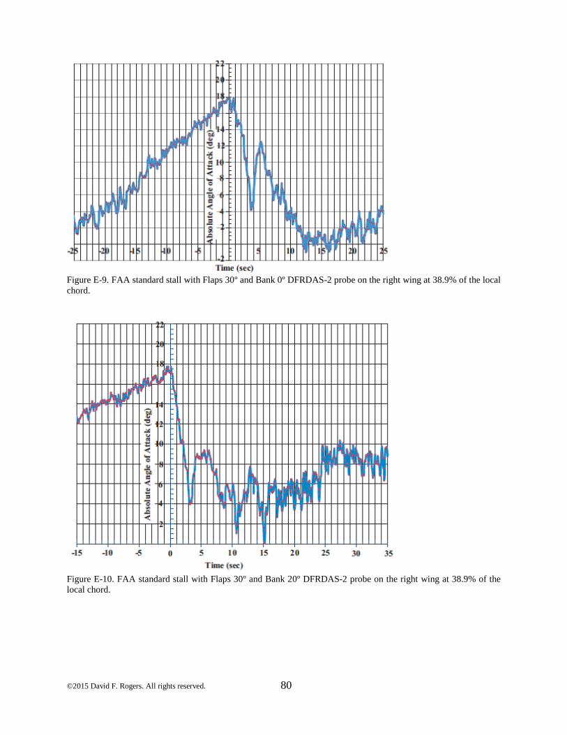
80 ©2015 David F. Rogers. All rights reserved.
Figure E-9. FAA standard stall with Flaps 30º and Bank 0º DFRDAS-2 probe on the right wing at 38.9% of the local
chord.
Figure E-10. FAA standard stall with Flaps 30º and Bank 20º DFRDAS-2 probe on the right wing at 38.9% of the
local chord.
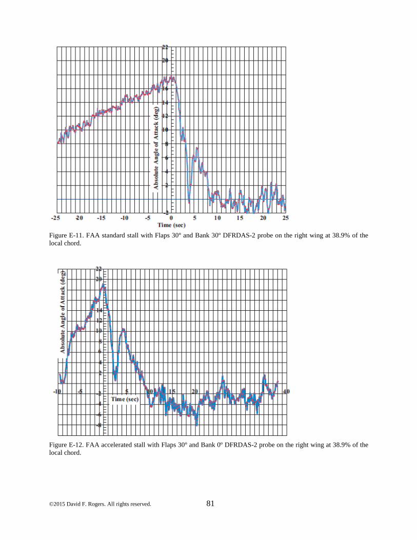
81 ©2015 David F. Rogers. All rights reserved.
Figure E-11. FAA standard stall with Flaps 30º and Bank 30º DFRDAS-2 probe on the right wing at 38.9% of the
local chord.
Figure E-12. FAA accelerated stall with Flaps 30º and Bank 0º DFRDAS-2 probe on the right wing at 38.9% of the
local chord.
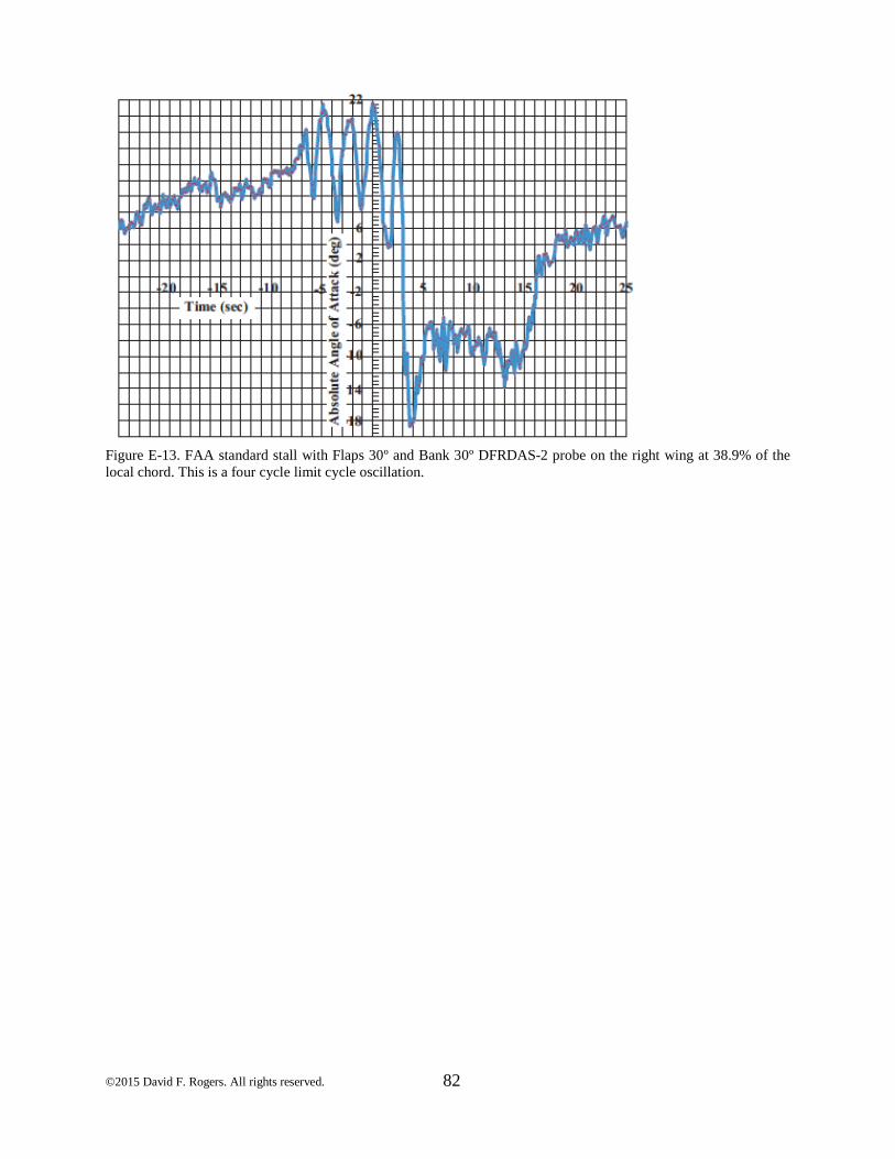
82 ©2015 David F. Rogers. All rights reserved.
Figure E-13. FAA standard stall with Flaps 30º and Bank 30º DFRDAS-2 probe on the right wing at 38.9% of the
local chord. This is a four cycle limit cycle oscillation.
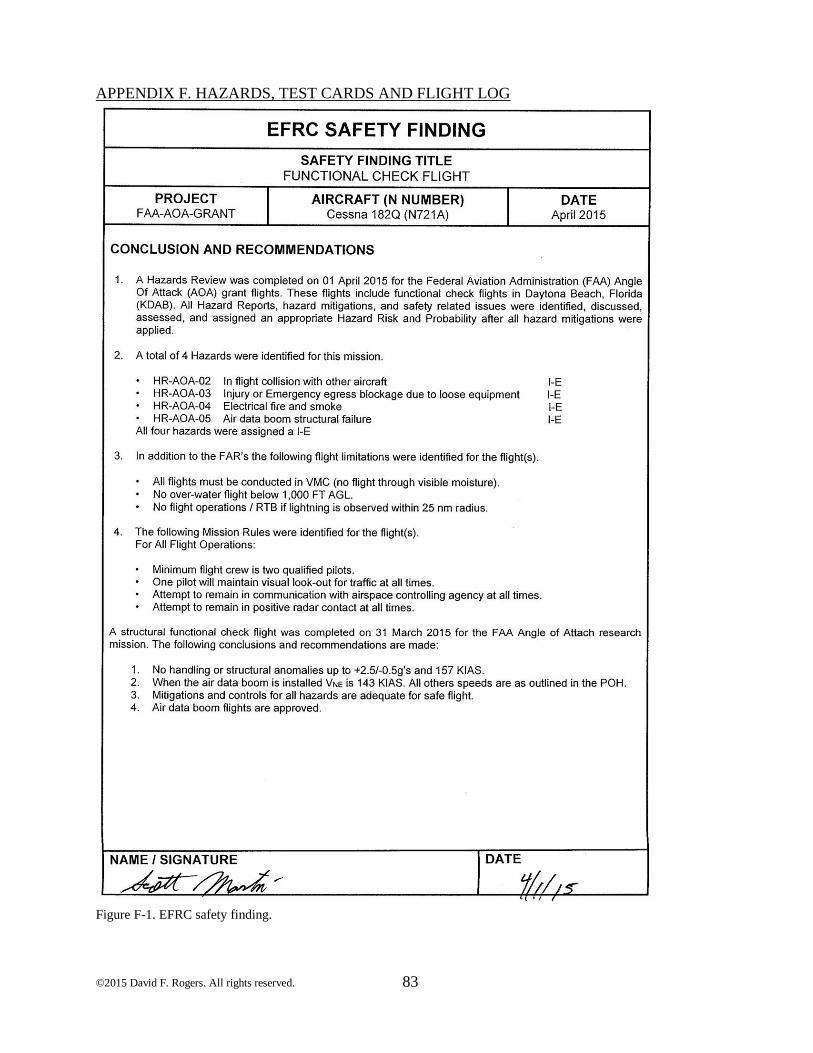
83 ©2015 David F. Rogers. All rights reserved.
APPENDIX F. HAZARDS, TEST CARDS AND FLIGHT LOG
Figure F-1. EFRC safety finding.
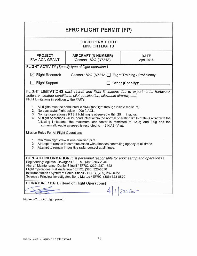
84 ©2015 David F. Rogers. All rights reserved.
Figure F-2. EFRC flight permit.
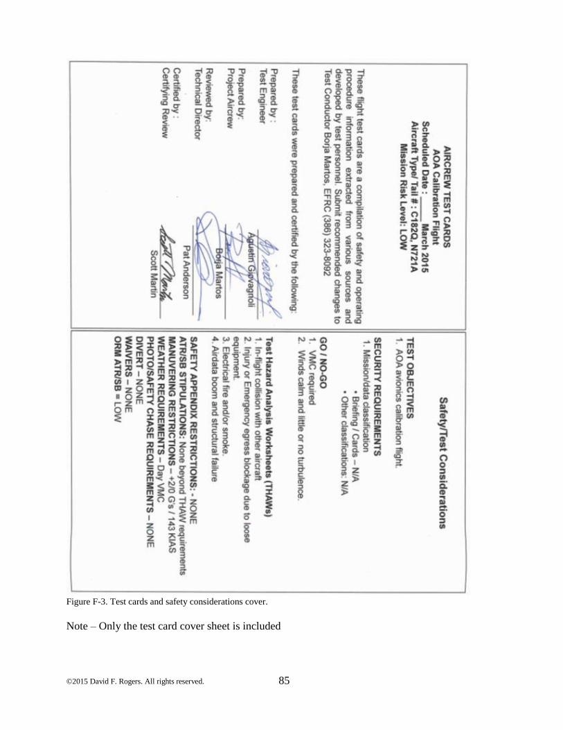
85 ©2015 David F. Rogers. All rights reserved.
Figure F-3. Test cards and safety considerations cover.
Note – Only the test card cover sheet is included

86 ©2015 David F. Rogers. All rights reserved.
HAZARD MATRIX AND SAFETY PROCESS
Figure F-4. Airworthiness and safety process.
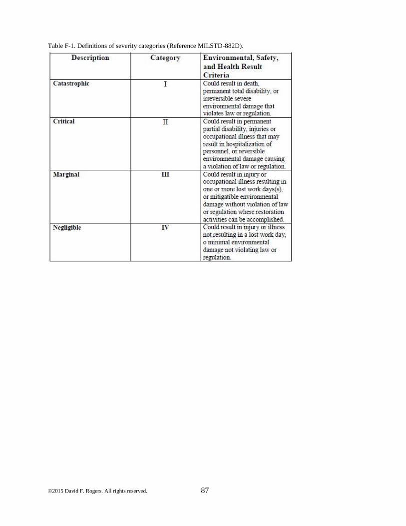
87 ©2015 David F. Rogers. All rights reserved.
Table F-1. Definitions of severity categories (Reference MILSTD-882D).

88 ©2015 David F. Rogers. All rights reserved.
Table F-2. Mishap probability levels (Reference MILSTD-882D).
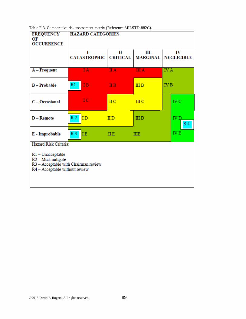
89 ©2015 David F. Rogers. All rights reserved.
Table F-3. Comparative risk assessment matrix (Reference MILSTD-882C).
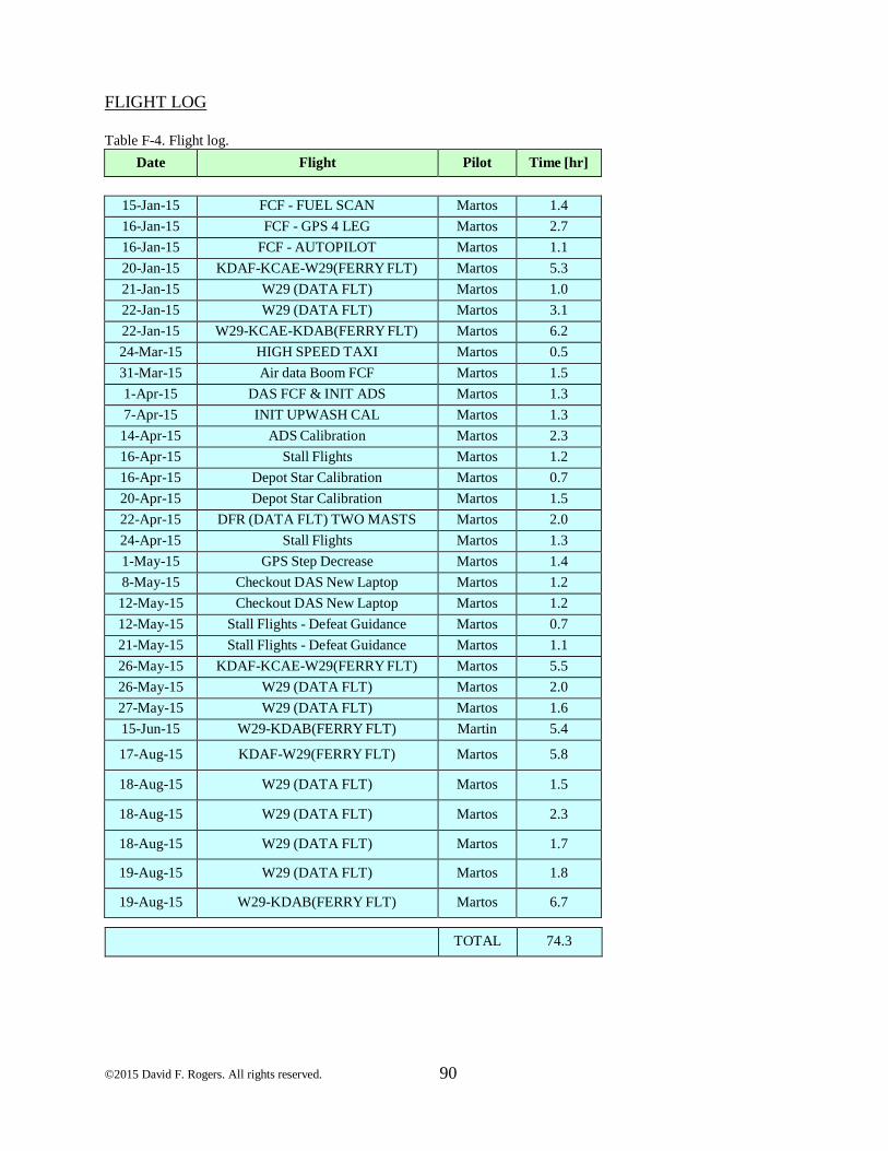
90 ©2015 David F. Rogers. All rights reserved.
FLIGHT LOG
Table F-4. Flight log.
Date Flight Pilot Time [hr]
15-Jan-15 FCF - FUEL SCAN Martos 1.4
16-Jan-15 FCF - GPS 4 LEG Martos 2.7
16-Jan-15 FCF - AUTOPILOT Martos 1.1
20-Jan-15 KDAF-KCAE-W29(FERRY FLT) Martos 5.3
21-Jan-15 W29 (DATA FLT) Martos 1.0
22-Jan-15 W29 (DATA FLT) Martos 3.1
22-Jan-15 W29-KCAE-KDAB(FERRY FLT) Martos 6.2
24-Mar-15 HIGH SPEED TAXI Martos 0.5
31-Mar-15 Air data Boom FCF Martos 1.5
1-Apr-15 DAS FCF & INIT ADS Martos 1.3
7-Apr-15 INIT UPWASH CAL Martos 1.3
14-Apr-15 ADS Calibration Martos 2.3
16-Apr-15 Stall Flights Martos 1.2
16-Apr-15 Depot Star Calibration Martos 0.7
20-Apr-15 Depot Star Calibration Martos 1.5
22-Apr-15 DFR (DATA FLT) TWO MASTS Martos 2.0
24-Apr-15 Stall Flights Martos 1.3
1-May-15 GPS Step Decrease Martos 1.4
8-May-15 Checkout DAS New Laptop Martos 1.2
12-May-15 Checkout DAS New Laptop Martos 1.2
12-May-15 Stall Flights - Defeat Guidance Martos 0.7
21-May-15 Stall Flights - Defeat Guidance Martos 1.1
26-May-15 KDAF-KCAE-W29(FERRY FLT) Martos 5.5
26-May-15 W29 (DATA FLT) Martos 2.0
27-May-15 W29 (DATA FLT) Martos 1.6
15-Jun-15 W29-KDAB(FERRY FLT) Martin 5.4
17-Aug-15 KDAF-W29(FERRY FLT) Martos 5.8
18-Aug-15 W29 (DATA FLT) Martos 1.5
18-Aug-15 W29 (DATA FLT) Martos 2.3
18-Aug-15 W29 (DATA FLT) Martos 1.7
19-Aug-15 W29 (DATA FLT) Martos 1.8
19-Aug-15 W29-KDAB(FERRY FLT) Martos 6.7
TOTAL 74.3