double chooz: outer veto detector
TRANSCRIPT

Double Chooz: Outer Veto Detector
Sophie BerkmanNevis Labs, Columbia University, New York, New York
(Dated: August 1, 2008)
This paper describes the work with photomultiplier tubes and scintillator strips done for theDouble Chooz project at Nevis Labs during the summer of 2008. The results described are a resultof tests of the hardware and software components as well as calibration procedures that will be usedto assemble the Double Chooz Outer Veto detector. It is done in preparation for the assembly ofthe final Outer Veto detector in Spring 2009.
1. INTRODUCTION
1.1. Standard Model of Particle Physics: A BriefOverview
The standard model of particle physics is currentlythe most comprehensive theory that describes elementaryparticles. It has been rigorously experimentally tested,but it still has shortcomings; for instance it still doesnot include the gravitational force, and does not describeneutrinos correctly.
FIG. 1: An illustration of the standard model of particlephysics. Shows the three families and two groups of particlesas well as the force carriers. The only particle not includedin this picture is the Higgs bozon [1].
The standard model contains three families of fermionswith spin 1
2 . These are broken into two groups; quarksand leptons. Quarks are fractionally charged and in-teract mainly through the strong force. They interactwith the strong force using their color charge. Thesequarks bind together to form hadrons like protons andneutrons. Since a fractional charge cannot exist indepen-dently, there are no free quarks. The up and down quarksare the ones that make protons and neutrons. The otherquarks include charm, strange, top and bottom. Thesesecond and third family quarks are unstable because theyquickly decay into less massive particles. Leptons, theother group, interact through all forces except the strong
interaction. This means that they are never bound insidea nucleus like quarks. Leptons include electrons, muons,taus and their associated neutrinos [2].
The standard model also describes the force carriers,or the mediators of the strong, weak and electromag-netic forces. The electromagnetic force is mediated bythe exchange of a massless photon. The strong force ismediated by gluons which couple to the color charge ofquarks, and the weak force is mediated by the chargedW and neutral Z bozons [3].
Neutrinos in the standard model are massless, charge-less, and come in three different flavors; electron, muonand tau. They interact only through the weak force andgravity, which makes them very hard to detect. Neu-trinos are left-handed particles, while antineutrinos areright-handed [2]. It currently an open question if theneutrino is a Dirac particle and there are right handedneutrinos and left-handed antineutrinos, or if in fact theneutrino is a Majorana particles so the neutrino is itsown antiparticle and the right-handed antineutrinos thathave been observed are actually right-handed neutrinos.One of the only ways to come to a conclusive solutionto this problem is to observe neutrinoless double betadecay which would confirm that neutrinos are Majoranaparticles. Also, neutrinos in the standard model cannotmix because their mass states and weak (flavor) statesare the same. The weak states are the wave functions ofthe particle that interact with the weak force, and themass states describe the mass of the neutrino. A resultof these conditions is that lepton family number is con-served. This conservation means that no neutrino typecan change into a neutrino of a different flavor [4].
1.2. Neutrino Oscillations
It has recently been shown that neutrinos oscillate,so in fact the neutrino flavor states are not the sameas the neutrino mass states. These were predicted byBruno Pontercorvo, and first observed by Ray Davis inhis Homestake mine experiment. In this experiment,Davis detected fewer solar neutrinos than predicted bythe theory. It was ultimately discovered that this neu-trino deficit was a result of neutrinos changing from oneflavor to another between their creation in the sun andtheir observation on Earth [4].

2
FIG. 2: The oscillation of a two neutrino system. ν1 and ν2are mass states, and νµ and νe are the flavor states. The redand blue waves are illustration of the two mass states, andthe purple wave is a combination of the two mass states intoa flavor state [5].
Since neutrinos oscillate, the current theory that hasnot been yet incorporated into the standard model givesneutrinos mass and violates lepton family number con-servation. This means that contrary to the description inthe standard model, electron neutrinos and muon neutri-nos and tau neutrinos can change into each other. Thishappens because the waves of the two mass states inter-fere with each other to form different flavor states; seefigure 2 for an illustration in the case of two neutrinos.The probability of oscillation in this two neutrino case isgiven by:
P (νµ → νe) = sin2(2θ)sin2(1.27∆m2L
E) (1)
where νµ and νe are the two neutrino flavors, θ is themixing angle, ∆m2 is the difference in the squares of theneutrino masses, L is the distance between the neutrinosource and the detector measuring neutrinos, and E isthe energy of the neutrinos. Using this formula it is pos-sible to choose L and E for optimal measurement of thedifferent mixing angles.
FIG. 3: The relationship between the neutrino mass and fla-vor eigenstates. [5].
In the three neutrino case, the mass and flavor statesare related by a unitary matrix as displayed in figure 3.This unitary matrix cam be broken into three other ma-trices, each characterized by a mixing angle, which is dis-played in figure 4. The first matrix, characterized by θ12was found by observing solar neutrino oscillations, as in
FIG. 4: [5].
Ray Davis’s experiment, and the third matrix was foundby observing atmospheric neutrino oscillations. The mid-dle matrix is described by θ13, which has not yet beenmeasured. Knowledge of this final mixing angle will helpus understand the relationship between the mass and fla-vor states of neutrinos. It will also allow investigationinto the δCP , which is a CP violation phase. This phasecould lead to an explanation about why there is morematter than antimatter in the universe [5].
1.3. Double Chooz
Double Chooz is a reactor experiment designed tomeasure the neutrino mixing angle θ13 [6]. Reactorexperiments look for a change in the flux of electron-antineutrinos as a function of the oscillation distance andthe energy (L and E). Electron-antineutrinos are createdas a result of fission of the isotopes U-235, U-238, Pu-239, Pu-241 in the reactor. The ultimate process that isdetected is inverse beta decay
ν̄ + p+ → n+ e+ (2)
which gives a double coincidence of first a positron sig-nal and then a neutron capture signal [7]. This doublecoincidence, within about 100µsec of each other, helpsto decrease the background of the experiment. Use of in-verse β decay means that effects from CP violation andmatter are negligible [5]. This will allow for a very pre-cise measurement of θ13. Double Chooz will be able tomeasure θ13 if the inequality 0.03 < sin2(2θ13) < 0.19holds [6]. This measurement of sin2(θ13) is expectedto be precise to within 0.03. A precise measurement of anon-zero θ13 will ultimately allow exploration of neutrinoCP-violation [6].
The experiment is located at the Chooz-B power sta-tion in France. This station operates two pressurizedwater reactors (PWR) which will both be used in the ex-periment. Detectors will be placed in two locations rela-tive to the reactors, one, the near detector will be located410m away, and the far detector will be at 1.05km. Thesedetectors will be virtually identical, with only a differentamount of outer shielding to account for the different cos-mic ray background at the two locations [6]. The near de-tector will detect the neutrino flux before oscillations oc-cur, while the far detector will detect neutrinos after os-cillations. If there are fewer electron-antineutrinos at the
3
far detector then an oscillation will have occurred. Theuse of two detectors will cancel uncertainties in neutrinoflux and the errors associated with the site choice [5].
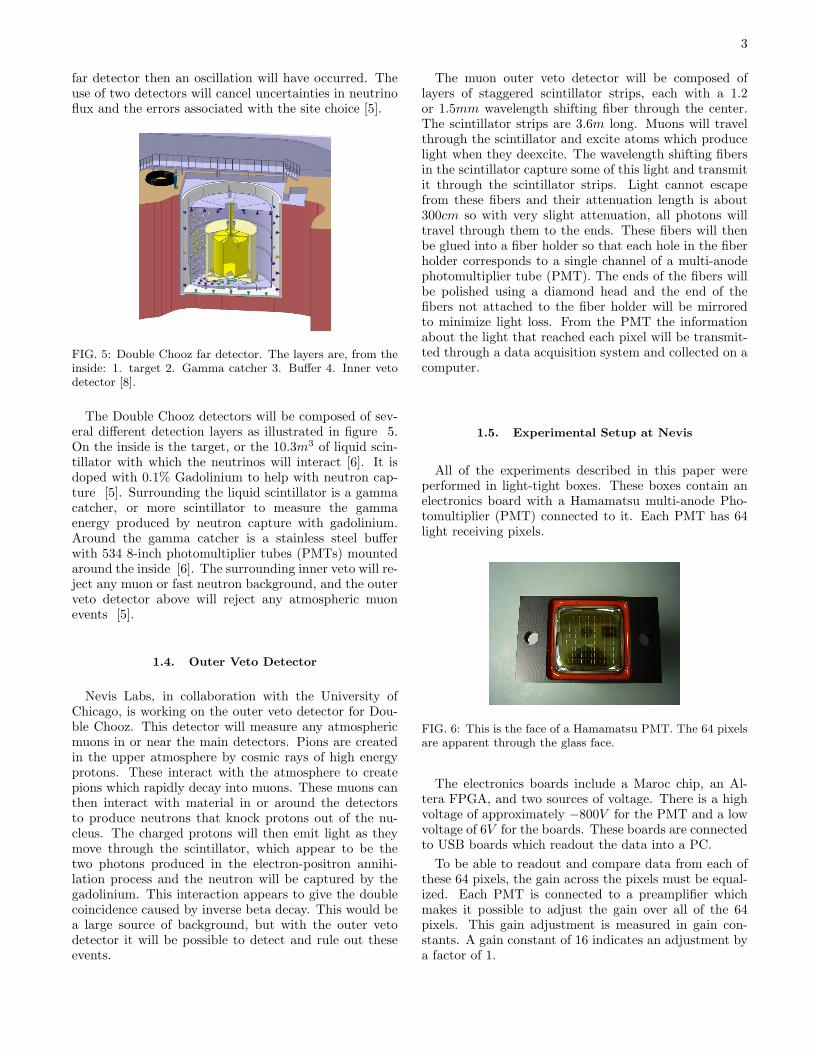
FIG. 5: Double Chooz far detector. The layers are, from theinside: 1. target 2. Gamma catcher 3. Buffer 4. Inner vetodetector [8].
The Double Chooz detectors will be composed of sev-eral different detection layers as illustrated in figure 5.On the inside is the target, or the 10.3m3 of liquid scin-tillator with which the neutrinos will interact [6]. It isdoped with 0.1% Gadolinium to help with neutron cap-ture [5]. Surrounding the liquid scintillator is a gammacatcher, or more scintillator to measure the gammaenergy produced by neutron capture with gadolinium.Around the gamma catcher is a stainless steel bufferwith 534 8-inch photomultiplier tubes (PMTs) mountedaround the inside [6]. The surrounding inner veto will re-ject any muon or fast neutron background, and the outerveto detector above will reject any atmospheric muonevents [5].
1.4. Outer Veto Detector
Nevis Labs, in collaboration with the University ofChicago, is working on the outer veto detector for Dou-ble Chooz. This detector will measure any atmosphericmuons in or near the main detectors. Pions are createdin the upper atmosphere by cosmic rays of high energyprotons. These interact with the atmosphere to createpions which rapidly decay into muons. These muons canthen interact with material in or around the detectorsto produce neutrons that knock protons out of the nu-cleus. The charged protons will then emit light as theymove through the scintillator, which appear to be thetwo photons produced in the electron-positron annihi-lation process and the neutron will be captured by thegadolinium. This interaction appears to give the doublecoincidence caused by inverse beta decay. This would bea large source of background, but with the outer vetodetector it will be possible to detect and rule out theseevents.
The muon outer veto detector will be composed oflayers of staggered scintillator strips, each with a 1.2or 1.5mm wavelength shifting fiber through the center.The scintillator strips are 3.6m long. Muons will travelthrough the scintillator and excite atoms which producelight when they deexcite. The wavelength shifting fibersin the scintillator capture some of this light and transmitit through the scintillator strips. Light cannot escapefrom these fibers and their attenuation length is about300cm so with very slight attenuation, all photons willtravel through them to the ends. These fibers will thenbe glued into a fiber holder so that each hole in the fiberholder corresponds to a single channel of a multi-anodephotomultiplier tube (PMT). The ends of the fibers willbe polished using a diamond head and the end of thefibers not attached to the fiber holder will be mirroredto minimize light loss. From the PMT the informationabout the light that reached each pixel will be transmit-ted through a data acquisition system and collected on acomputer.
1.5. Experimental Setup at Nevis
All of the experiments described in this paper wereperformed in light-tight boxes. These boxes contain anelectronics board with a Hamamatsu multi-anode Pho-tomultiplier (PMT) connected to it. Each PMT has 64light receiving pixels.
FIG. 6: This is the face of a Hamamatsu PMT. The 64 pixelsare apparent through the glass face.
The electronics boards include a Maroc chip, an Al-tera FPGA, and two sources of voltage. There is a highvoltage of approximately −800V for the PMT and a lowvoltage of 6V for the boards. These boards are connectedto USB boards which readout the data into a PC.
To be able to readout and compare data from each ofthese 64 pixels, the gain across the pixels must be equal-ized. Each PMT is connected to a preamplifier whichmakes it possible to adjust the gain over all of the 64pixels. This gain adjustment is measured in gain con-stants. A gain constant of 16 indicates an adjustment bya factor of 1.

4
2. PMT CHARACTERIZATION
The six Hamamatsu photomultiplier tubes (PMTs)were characterized so that all of the PMTs will respondin the same way to incident light. It is expected that eachpixel will receive 10 photoelectrons from atmosphericmuons, and preliminary studies show that there are ap-proximately 35 ADC counts per photoelectron. Thismeans that the mean pulse height of each PMT pixelshould be adjusted to 350 ADC counts for the most uni-form reading. These PMTs were tested with a varietyof electronics boards because in the Double Chooz ex-periment each PMT will be characterized individually toits own electronics board. The information about whichPMT was tested with which electronics board is in Ta-ble I.
PMT serial # Electronics Board # HV after Adjustment (V)
PA4662 4 795
PA4665 4 804
PA4674 4 785
PA4653 6 802
PA4663 3 785
PA4660 5 830
TABLE I: This table displays the setup of the PMTs andexperimental characterization high voltage.
A Picoquant pulsed LED laser was used to send lightpulses to the PMT and simulate muon events. This typeof laser was used because the pulses are very precise.
Data from the characterization process was collectedusing the Perl program pmtcharacterization. This pro-gram walks the user through the procedure described be-low, and also independently takes data related to theDAC threshold, as well as the number of photoelectronsthat hit each pixel on the PMT.
The following procedure is the one used in the PMTcharacterization process to adjust the mean pulse heightof each pixel to 350 ADC counts.
1. Data is taken with the laser off to get a reading ofthe baseline pulses. The baseline is a reading of thepulses when no signal is sent to the electronics.
2. The laser is turned on and stabilizes for 30 minutesto get a consistent laser pulse.
3. The high voltage is adjusted to get a mean pulseheight of 350 ADC counts for all of the pixels.
4. The gain constant of the preamplifier for each indi-vidual pixel is adjusted to yield a mean pulse heightof 350 ADC counts for each pixel.
5. The laser is turned off and the PMT is allowed tosettle for 30 minutes.
ADC100 200 300 400 500 600 700
Coun
t
0
20
40
60
80
100
120
140
160
180
200
Before the Pixel Adjustment h1Entries 384Mean 348.9RMS 63.54
Before the Pixel Adjustment
h1Entries 384Mean 348.9RMS 63.54
ADC100 200 300 400 500 600 700
Coun
t
0
20
40
60
80
100
120
140
160
180
200 h1Entries 384Mean 348.9RMS 63.54
Before the Pixel Adjustment
h1Entries 384Mean 348.9RMS 63.54
ADC100 200 300 400 500 600 700
Coun
t
0
20
40
60
80
100
120
140
160
180
200 h1Entries 384Mean 348.9RMS 63.54
Before the Pixel Adjustment
FIG. 7: Histogram of the pulse heights in the six PMTs afterthe high voltage adjustment, but before the pixel adjustment.
6. Noise rate data is taken for several DAC thresholds;13 , 2
3 , 1, 2 photoelectrons.
7. The program HV analysis.pl is used to extract thepulse height data from the files created during thecharacterization process.
After this procedure was repeated for the six PMTs,the distribution of pulse heights was plotted, using theprogram plotall.C, to make histograms of the pulse heightof the light after the high voltage adjustment and afterthe gain adjstment. The program finalhist.C was usedto format the histograms. There are histograms for eachindividual PMT, as well as a histogram that is the sumof the pulse height distributions in both conditions. Thedistribution of pulse heights is much narrower after thecharacterization and is centered around 350 ADC counts.Before the pixel adjustment, the spread around 350 ADCcounts is from 260-540 ADC counts, and after the pixeladjustment, the spread is from 330-370 ADC counts.
ADC100 200 300 400 500 600 700
Co
un
t
0
20
40
60
80
100
120
140
160
180
200
After the Characterization h1Entries 384Mean 349.9RMS 9.979
/ ndf 2! 10.96 / 5
Prob 0.0522Constant 13.6! 199.8 Mean 0.4! 349.7 Sigma 0.335! 7.467
After the Characterization
h1Entries 384
Mean 349.9RMS 9.979
/ ndf 2! 10.96 / 5
Prob 0.0522Constant 13.6! 199.8
Mean 0.4! 349.7 Sigma 0.335! 7.467
ADC100 200 300 400 500 600 700
Co
un
t
0
20
40
60
80
100
120
140
160
180
200h1
Entries 384
Mean 349.9RMS 9.979
/ ndf 2! 10.96 / 5
Prob 0.0522Constant 13.6! 199.8
Mean 0.4! 349.7 Sigma 0.335! 7.467
After the Characterization
FIG. 8: Histogram of the pulse heights in the six PMTs afterthe characterization process.

5
ADC300 310 320 330 340 350 360 370 380 390 400
Coun
t
0
5
10
15
20
25
30
35
40
45
50After the Characterization h1
Entries 384Mean 349.5RMS 7.799Underflow 0Overflow 2
/ ndf 2! 92.95 / 24Prob 4.656e-010Constant 2.17± 26.22 Mean 0.4± 347.5 Sigma 0.456± 6.517
After the Characterization
h1Entries 384Mean 349.5RMS 7.799Underflow 0Overflow 2
/ ndf 2! 92.95 / 24Prob 4.656e-010Constant 2.17± 26.22 Mean 0.4± 347.5 Sigma 0.456± 6.517
ADC300 310 320 330 340 350 360 370 380 390 400
Coun
t
0
5
10
15
20
25
30
35
40
45
50 h1Entries 384Mean 349.5RMS 7.799Underflow 0Overflow 2
/ ndf 2! 92.95 / 24Prob 4.656e-010Constant 2.17± 26.22 Mean 0.4± 347.5 Sigma 0.456± 6.517
After the Characterization
FIG. 9: A zoomed in histogram of the pulse heights in the sixPMTs after the characterization process.
Gain Constants (a.u.)5 10 15 20 25 30 35 40
Nu
mb
er
of
Oc
cu
rre
nc
es
0
10
20
30
40
50
Distribution of Gain Constants all_gains
Entries 384Mean 16.6
RMS 2.9Underflow 0
Overflow 0 / ndf 2χ 30.41 / 10
Prob 0.0007335Constant 3.49± 46.42 Mean 0.20± 17.33 Sigma 0.213± 3.191
Distribution of Gain Constants
all_gains
Entries 384Mean 16.6RMS 2.9Underflow 0Overflow 0
/ ndf 2χ 30.41 / 10Prob 0.0007335Constant 3.49± 46.42 Mean 0.20± 17.33 Sigma 0.213± 3.191
Gain Constants (a.u.)5 10 15 20 25 30 35 40
Nu
mb
er
of
Oc
cu
rre
nc
es
0
10
20
30
40
50
all_gains
Entries 384Mean 16.6RMS 2.9Underflow 0Overflow 0
/ ndf 2χ 30.41 / 10Prob 0.0007335Constant 3.49± 46.42 Mean 0.20± 17.33 Sigma 0.213± 3.191
Distribution of Gain Constants
FIG. 10: Histogram of the distribution of gain constants afterthe characterization.
Figures 7 and 8 show before and after the pixel ad-justment plotted on the same scale. Figure 9 is a versionof figure 8 with a more appropriate scale and binning tomake it possible to see the variations in the pulse heightdistribution after the characterization more clearly.
For this same characterization, the distribution of gainconstants was also plotted in figure 10. The gain con-stants give the factor of adjustment that must be madein the preamplifier so that each pixel will respond to lightin the same way. The distribution of these adjustmentsis similar to the distribution of pulse heights after thecharacterization process.
3. PRELIMINARY SCINTILLATOREXPERIMENTS
3.1. Scintillator Setup
Four scintillator strips of 1.5m were put together in asimulation of the muon outer veto detector for Double
FIG. 11: Picture of the scintillator setup. TU1 indicates ”up-per trigger counter 1” , TU1 indicates ”lower trigger counter1”, etc for the rest of the trigger counters.
Name Maroc Channel Distance to PMT (cm)
TC TU1 58 170
TD1 57 170
TU2 50 122
TD2 49 122
TU3 42 75
TD3 41 75
TU4 34 33
TD4 33 33
Strips S1 64
S2 54
S3 40
S4 37
TABLE II: Several properties of the scintillator setup are de-scribed in this Table. First, the mapping of all of the stripsand trigger counters onto Maroc channels. The Maroc chan-nel number can be expressed in terms of PMT channel usingthe expression: ChannelMaroc = 64 − ChannelPMT . It alsodisplays the distance from the trigger counters, or positions,to the PMT.
Chooz. These strips were stacked on top of each otherwith four trigger counters affixed above and four triggercounters affixed below them. These trigger counters are4.5cm by 5.0cm pieces of scintillator. They are arrangedin groups of two, one above the scintillator strips and onebelow the scintillator strips as illustrated in Figure 11.The location and number of the trigger counters indicatethe different positions relative to the PMT. All of thepieces are held together with electrical tape. Wavelengthshifting fiber of 1.2mm in diameter was threaded througheach piece of scintillator and each trigger counter. Thesewere then mapped into different holes in a fiber holder.The fiber holder has a face with 64 holes, and each holecorresponds to one pixel of the PMT. This means thatthe light from each strip, and trigger counter can be mea-sured individually by looking at the light in an individualPMT pixel. Table II gives the mapping of the fibers inthe PMT board. All of the fibers are in channels 32-64because these locations in the fiber-holder are designedto hold 1.2mm fibers, while the other 32 slots are de-

6
signed to hold 1.5mm fibers. It has not yet been decidedwhich size fiber Double Chooz will use. The fibers wereglued into the fiber holder, and the ends were polishedusing sandpaper of several different grades. This was animperfect polishing; there were still some small scratchesin the ends of the fibers. In the final experiment theends of the fibers will be polished with a diamond headto maximize the light that will be transmitted from thefibers to the PMT.
For some of the following experiments a spacer wasused between the fiber holder and the glass face of thePMT. This was implemented to protect the PMT af-ter a PMT was broken because the fiber holder was at-tached too tightly to the PMT, and the glass face cracked.There are two different sizes of spacer: the large spaceris 2.38mm and the small spacer is 1.60mm. When aspacer is used there is an air gap between the ends of thefibers and the PMT face. For the large spacer this gapis 1.27mm, and for the small spacer it is 0.483mm. Op-tical grease was also used between the face of the PMTand the fibers in some cases to increase the number ofphotoelectrons that the PMT received from the fibers.
3.2. Efficiency Measurements
To do a preliminary study the efficiency of the scin-tillator strips, the pulse height in strip 1 was measuredwith different trigger coincidence requirements to definea muon event. All of them required that strip 1 have anonzero pulse height, as well as:
1. 1. Both TU4 and TD4 have a pulse height of atleast 1 photoelectron.
2. 2. TU4, TD4 and strip 2 have pulse heights of atleast 1 photoelectron.
3. 3. TU4, TD4, strip 2 and strip 3 have pulse heightsof at least 1 photoelectron.
4. 4. TU4, TD4, strip2, strip3 and strip 4 have pulseheights of at least 1 photoelectron.
All of these measurements were taken at position 4,closest to the PMT to get the most events and highestpulse heights, and was done using spacers of both2.38mmand 1.60mm.
The pulse height distributions under these four differ-ent coincidences are displayed in figures 12 through 15.
The mean pulse heights with these different coinci-dence requirements are all very similar, the range is lessthan 4 ADC counts, from 150.5 to 154.1 ADC counts.The number of events, however changes significantly asmore coincidences are required.
The efficiency can be calculated using the formula
E =Number of Entriesafter cutNumber of Entriesbefore cut
(3)
h1Entries 359Mean 180.6RMS 111.9
ADC0 100 200 300 400 500 600 700
Coun
ts
0
5
10
15
20
25
30
h1Entries 359Mean 180.6RMS 111.9
Strip 1 with events in TU4 and TD4 above 1pe- using small spacer
FIG. 12: Histogram of strip 1 requiring that there are eventsin TU4 and TD4.
h1Entries 326Mean 184.4RMS 109
ADC0 100 200 300 400 500 600 700
Coun
ts
0
5
10
15
20
25
30h1
Entries 326Mean 184.4RMS 109
Strip 1 with events in S2, TU4 and TD4 above 1pe- using small spacer
FIG. 13: Histogram of strip 1 requiring that there are eventsin strip 2, TU4 and TD4.
h1Entries 306Mean 184.3RMS 109.2
ADC0 100 200 300 400 500 600 700
Coun
ts
0
5
10
15
20
25
h1Entries 306Mean 184.3RMS 109.2
Strip 1 with events in S2, S3, TU4 and TD4 above 1pe- using small spacer
FIG. 14: Histogram of strip 1 requiring that there are eventsin strip 2, strip 3, TU4 and TD4.

7
h1Entries 294Mean 183.3RMS 109.2
ADC0 100 200 300 400 500 600 700
Coun
ts
0
5
10
15
20
25
h1Entries 294Mean 183.3RMS 109.2
Strip 1 with events in S2, S3, S4, TU4 and TD4 above 1pe- using small spacer
FIG. 15: Histogram of strip 1 requiring that there are eventsin strip 2, strip 3, strip 4, TU4 and TD4.
The efficiencies are displayed in table III. The efficien-cies increase by about 10% with the smaller spacer. Thisis probably a result of less diffraction in the light withless space between the ends of the fibers and the face ofthe PMT.
The number of photoelectrons can be calculated usingthe inefficiency and the formula
1− E = e−µ (4)
where E is the efficiency of the strip, and µ is the num-ber of photoelectrons. It is based on the inefficiency be-cause it depends on the quantity 1 − E. This formuladerives from the Poisson distribution and predicts thenumber of photoelectrons for a given efficiency. It is alsopossible to find the number of photoelectrons directlyfrom the experimental data by using the conversion of35 ADC counts is 1 photoelectron. This data is also dis-played in Table III.
The number of photoelectrons predicted by the Pois-son distribution and calculated directly from the meanpulse height are very different. This is probably a resultof the fact that the air gap between the ends of the fibersand the PMT introduce factors that do not follow thedistribution. It is also possible that there is significantcross talk between the pixels that significantly lowers thenumber of photoelectrons in the signal pixel that is ex-amined. This could be better examined by testing all ofthe triggers and strips at every position, as well as ex-amining the efficiency for the data runs taken without aspacer and with optical grease.
3.3. Photoelectron Measurements and Cross Talk
The pulse heights in the efficiency measurements weremuch smaller, around 5 photoelectrons than the ones of
10 photoelectrons expected. This effect was partially dueto crosstalk between the pixels, so the pulses from thepixels surrounding the central pixel were added into thepulse height of the pixel receiving the signal. There aredifferent numbers of surrounding pixels for some of thestrips; strip 1 has 3 neighbors, strip 3 has 5 neighbors andstrips 2 and 4 both have 8 neighbors. The light pulses ofthe surrounding pixels were added into the signal pixelonly when there was a trigger in the central pixel andthe surrounding pixel, and the pulse in the surroundingpixel was at least 1
16 photoelectron. This cut was meantto restrict the amount of noise added back in as events.This procedure was performed for all four strips at allfour positions to find the maximum pulse heights if thereis no cross talk.
The pulse height distribution was plotted before andafter the surrounding pixel addition. They were fit-ted with a landau-gaussian distribution to find the mostprobable value.
An example of this plot is displayed in figure 16. Theratio of the most probable value before the pixel additionto the most probable value after the pixel addition isthe percentage of light that stayed in the signal pixel.This means that subtracting this ratio from one givesthe crosstalk fraction.
These values for the cross talk from runs with the smallspacer, no spacer and no spacer with optical grease aredisplayed in table V.
The cross talk is generally greatest for the run withthe small spacer, where it is sometimes as much as 24%.This may account for the low number of photoelectronsin the previous study.
3.4. Effect of position on Mean Pulse Height
In this study, we examined the effects of position on themean pulse heights of the pixels on a PMT. This was doneby finding the mean pulse height of each strip, and eachtrigger at four different positions. These positions are thelocations of the trigger counters on the four scintillatorstrips. Table ?? indicates the distances from the PMTto each position.
Each of these required a five-fold coincidence for eachpulse height measurement. This means that for eachmeasurement one strip is selected as the signal-strip, andthen all of the other strips and trigger counters at thatposition are required to have a response of at least 1photoelectron. This is done for each strip at each of thefour positions. Data from three different runs was exam-ined. All of them use optical grease without a spacer.Run 20080710 6 was taken using trigger mode 0, whileRuns 20080710 7 and 20080716 0 were taken using trig-ger mode 2. Trigger mode 0 accepts an event if any trig-ger or strip is over the DAC threshold. Trigger mode 2accepts events only if two paired trigger counters bothrecord an event over the DAC threshold. A selection ofthe plots that were created from this data are displayed
8
Cut Entries before Cut Entries after Cut Efficiency(%) #PE Poisson # PE from PH
Large Spacer: S2,Triggers 312 258 83 1.77 4.3
S2, S3,Triggers 258 215 83 1.77 4.44
S2,S3,S4,Triggers 215 194 90 2.30 4.40
Small spacer: S2,Triggers 359 326 91 2.40 5.27
S2, S3,Triggers 326 306 94 2.81 5.27
S2,S3,S4,Triggers 306 294 96 3.23 5.24
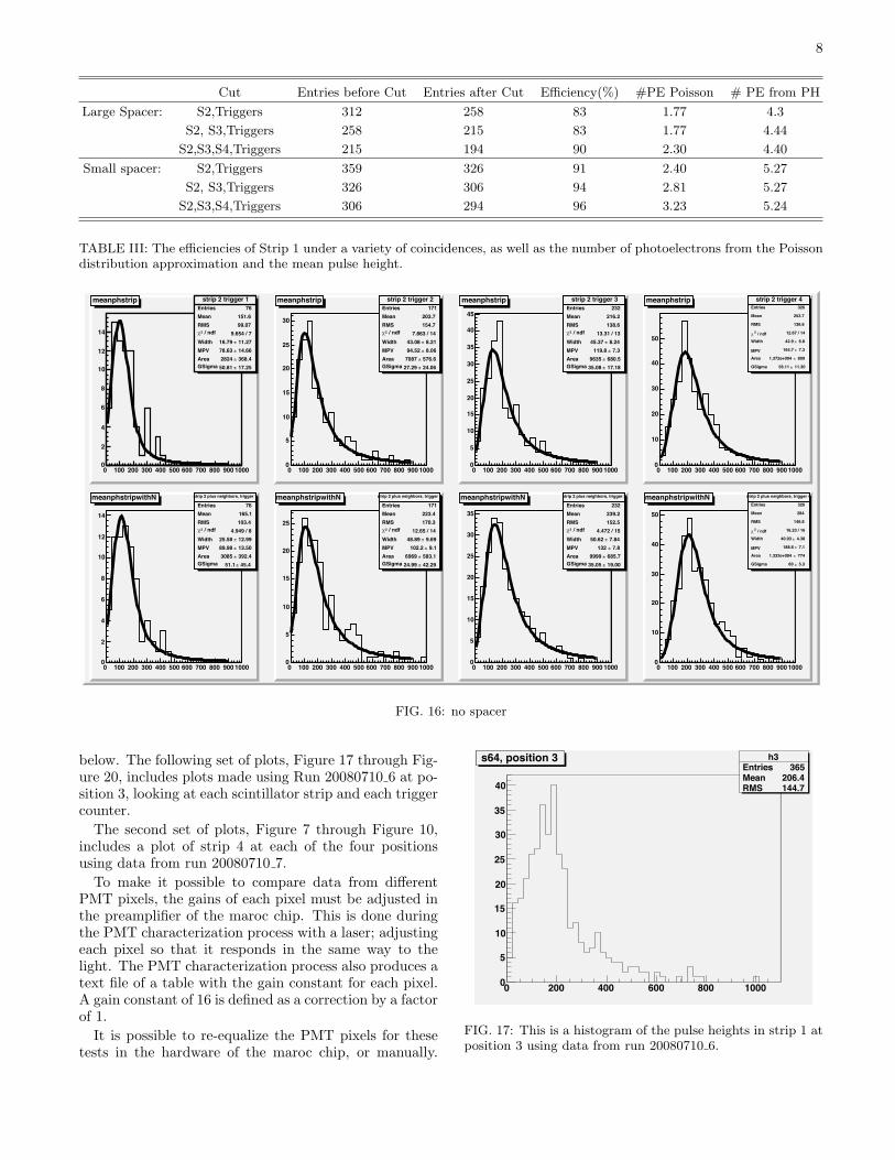
TABLE III: The efficiencies of Strip 1 under a variety of coincidences, as well as the number of photoelectrons from the Poissondistribution approximation and the mean pulse height.
strip 2 trigger 1Entries 76Mean 151.6RMS 99.07
/ ndf 2χ 9.654 / 7Width 11.27± 16.79 MPV 14.66± 78.63 Area 368.4± 2824 GSigma 17.25± 50.81
0 100 200 300 400 500 600 700 800 900 10000
2
4
6
8
10
12
14
strip 2 trigger 1Entries 76Mean 151.6RMS 99.07
/ ndf 2χ 9.654 / 7Width 11.27± 16.79 MPV 14.66± 78.63 Area 368.4± 2824 GSigma 17.25± 50.81
meanphstrip strip 2 trigger 2Entries 171Mean 203.7RMS 154.7
/ ndf 2χ 7.863 / 14Width 8.21± 43.08 MPV 8.06± 94.52 Area 576.6± 7087 GSigma 24.06± 27.29
0 100 200 300 400 500 600 700 800 900 10000
5
10
15
20
25
30
strip 2 trigger 2Entries 171Mean 203.7RMS 154.7
/ ndf 2χ 7.863 / 14Width 8.21± 43.08 MPV 8.06± 94.52 Area 576.6± 7087 GSigma 24.06± 27.29
meanphstrip strip 2 trigger 3Entries 232Mean 216.2RMS 138.6
/ ndf 2χ 13.31 / 13Width 8.24± 45.37 MPV 7.3± 119.8 Area 680.5± 9635 GSigma 17.18± 35.08
0 100 200 300 400 500 600 700 800 900 10000
5
10
15
20
25
30
35
40
45
strip 2 trigger 3Entries 232Mean 216.2RMS 138.6
/ ndf 2χ 13.31 / 13Width 8.24± 45.37 MPV 7.3± 119.8 Area 680.5± 9635 GSigma 17.18± 35.08
meanphstrip strip 2 trigger 4Entries 326
Mean 253.7
RMS 136.6
/ ndf 2χ 12.67 / 14
Width 6.8± 42.9
MPV 7.3± 164.7
Area 809± 1.372e+004
GSigma 11.30± 56.11
0 100 200 300 400 500 600 700 800 900 10000
10
20
30
40
50
strip 2 trigger 4Entries 326
Mean 253.7
RMS 136.6
/ ndf 2χ 12.67 / 14
Width 6.8± 42.9
MPV 7.3± 164.7
Area 809± 1.372e+004
GSigma 11.30± 56.11
meanphstrip
strip 2 plus neighbors, trigger 1
Entries 76Mean 165.1RMS 103.4
/ ndf 2χ 4.949 / 8Width 12.99± 25.58 MPV 13.50± 89.98 Area 392.4± 3085 GSigma 45.4± 51.1
0 100 200 300 400 500 600 700 800 900 10000
2
4
6
8
10
12
14
strip 2 plus neighbors, trigger 1
Entries 76Mean 165.1RMS 103.4
/ ndf 2χ 4.949 / 8Width 12.99± 25.58 MPV 13.50± 89.98 Area 392.4± 3085 GSigma 45.4± 51.1
meanphstripwithN strip 2 plus neighbors, trigger 2
Entries 171Mean 223.4RMS 170.3
/ ndf 2χ 12.65 / 14Width 9.69± 48.89 MPV 9.1± 102.2 Area 583.1± 6969 GSigma 42.29± 24.99
0 100 200 300 400 500 600 700 800 900 10000
5
10
15
20
25
strip 2 plus neighbors, trigger 2
Entries 171Mean 223.4RMS 170.3
/ ndf 2χ 12.65 / 14Width 9.69± 48.89 MPV 9.1± 102.2 Area 583.1± 6969 GSigma 42.29± 24.99
meanphstripwithN strip 2 plus neighbors, trigger 3
Entries 232Mean 239.2RMS 152.5
/ ndf 2χ 4.472 / 15Width 7.84± 50.62 MPV 7.8± 132 Area 685.7± 9999 GSigma 19.00± 35.05
0 100 200 300 400 500 600 700 800 900 10000
5
10
15
20
25
30
35
strip 2 plus neighbors, trigger 3
Entries 232Mean 239.2RMS 152.5
/ ndf 2χ 4.472 / 15Width 7.84± 50.62 MPV 7.8± 132 Area 685.7± 9999 GSigma 19.00± 35.05
meanphstripwithN strip 2 plus neighbors, trigger 4
Entries 326
Mean 284
RMS 146.8
/ ndf 2χ 16.23 / 16
Width 4.38± 40.93
MPV 7.1± 188.6
Area 774± 1.332e+004
GSigma 5.3± 60
0 100 200 300 400 500 600 700 800 900 10000
10
20
30
40
50
strip 2 plus neighbors, trigger 4
Entries 326
Mean 284
RMS 146.8
/ ndf 2χ 16.23 / 16
Width 4.38± 40.93
MPV 7.1± 188.6
Area 774± 1.332e+004
GSigma 5.3± 60
meanphstripwithN
FIG. 16: no spacer
below. The following set of plots, Figure 17 through Fig-ure 20, includes plots made using Run 20080710 6 at po-sition 3, looking at each scintillator strip and each triggercounter.
The second set of plots, Figure 7 through Figure 10,includes a plot of strip 4 at each of the four positionsusing data from run 20080710 7.
To make it possible to compare data from differentPMT pixels, the gains of each pixel must be adjusted inthe preamplifier of the maroc chip. This is done duringthe PMT characterization process with a laser; adjustingeach pixel so that it responds in the same way to thelight. The PMT characterization process also produces atext file of a table with the gain constant for each pixel.A gain constant of 16 is defined as a correction by a factorof 1.
It is possible to re-equalize the PMT pixels for thesetests in the hardware of the maroc chip, or manually.
0 200 400 600 800 10000
5
10
15
20
25
30
35
40
s64, position 3 h3Entries 365Mean 206.4RMS 144.7
s64, position 3
FIG. 17: This is a histogram of the pulse heights in strip 1 atposition 3 using data from run 20080710 6.
9
0 200 400 600 800 10000
5
10
15
20
25
30
s54, position 3 h3Entries 349Mean 281.7RMS 158.5
s54, position 3
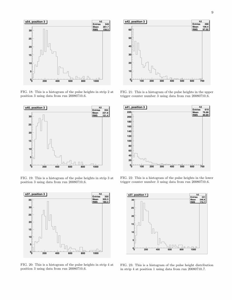
FIG. 18: This is a histogram of the pulse heights in strip 2 atposition 3 using data from run 20080710 6.
0 200 400 600 800 10000
5
10
15
20
25
30
s40, position 3 h3Entries 354Mean 221.8RMS 151.4
s40, position 3
FIG. 19: This is a histogram of the pulse heights in strip 3 atposition 3 using data from run 20080710 6.
0 200 400 600 800 10000
5
10
15
20
25
30
35
s37, position 3 h3Entries 350Mean 305.3RMS 180.4
s37, position 3
FIG. 20: This is a histogram of the pulse heights in strip 4 atposition 3 using data from run 20080710 6.
0 100 200 300 400 500 600 7000
10
20
30
40
50
60
s42, position 3 h3Entries 468Mean 106.4RMS 97.02
s42, position 3
FIG. 21: This is a histogram of the pulse heights in the uppertrigger counter number 3 using data from run 20080710 6.
0 100 200 300 400 500 600 7000
20
40
60
80
100
120
140
160
180
200
220
s41, position 3 h3Entries 619Mean 76.88RMS 89.89
s41, position 3
FIG. 22: This is a histogram of the pulse heights in the lowertrigger counter number 3 using data from run 20080710 6.
0 200 400 600 800 10000
5
10
15
20
25
30
s37, position 1 h3Entries 331Mean 246.8RMS 172.7
s37, position 1
FIG. 23: This is a histogram of the pulse height distributionin strip 4 at position 1 using data from run 20080710 7.

10
0 200 400 600 800 10000
10
20
30
40
50
s37, position 2 h3Entries 618Mean 269.9RMS 166.4
s37, position 2
FIG. 24: This is a histogram of the pulse height distributionin strip 4 at position 2 using data from run 20080710 7.
0 200 400 600 800 10000
10
20
30
40
50
60
70
s37, position 3 h3Entries 913Mean 308.3RMS 170.2
s37, position 3
FIG. 25: This is a histogram of the pulse height distributionin strip 4 at position 3 using data from run 20080710 7.
0 200 400 600 800 10000
10
20
30
40
50
60
s37, position 4 h3Entries 1019Mean 355.1RMS 181.7
s37, position 4
FIG. 26: This is a histogram of the pulse height distributionin strip 4 at position 4 using data from run 20080710 7.
To use the hardware, the gain constant files producedin the PMT characterization must be reloaded into themaroc chip from the characterization data. This is theprocess used to correct for the gain differences in PMTpixels for run 20080716 0. The manual correction is doneby using the correction for each pixel recorded in thetext file. The gain constant is divided by 16 to find thecorrection factor, and this factor is then multiplied bythe mean pulse height measured. This manual correctionwas performed for runs 20080710 6 and 20080710 7. Forthese two runs data is included with and without thecorrection; the before column indicates the mean pulseheight before the gain correction and the after columnindicates the mean pulse height after the gain correction.All of the plots displayed include data from before thisgain correction. The mean pulse heights of all of thestrips and trigger counters at the different positions aredisplayed in Table VI.
From these data tables, there are several conclusionsthat can be drawn. It is first important to note thatthe absolute pulse height is very different for each of thestrips. Strip 2 and Strip 4 both have a similar range ofpulse heights, 250-400 ADC counts, after the gain cor-rection. Strip 1 has the lowest pulse heights, from about115 to 200 ADC counts after gain correction, while strip3 is somewhere in between with a range of 160 to 250ADC counts after gain correction. Since this gain cor-rection equalizes the PMT pixels so that they respondin the same way to light, the discrepancy in pulse heightis probably the result of differences in the scintillator orthe polishing of the wavelength shifting fibers.
The pulse height also increases for each strip in posi-tions closer to the PMT. This increase is about 70-150ADC counts from the position farthest away from thePMT (Position 1) and the position closest to the PMT(Position 4). The amount of increase over the positionsis similar for all of the strips, except for small deviationsin Strip 3. This is to be expected because in positionscloser to the PMT more of the light in the scintillatorwill reach the PMT. This is a result of the attenuationlength of the optical fibers. This increased pulse height isalso apparent in the trigger counters. This data can alsobe used to calculate the attenuation length of the opticalfibers, and this is a subsequent analysis that should beperformed.
The trigger counters also have much lower pulseheights than the strips. They are generally 100-200 ADCcounts smaller than the scintillator strips. The length ofwavelength shifting fiber available to collect scintillationlight is smaller in the trigger counters, so light may belost due muons hitting the scintillator at the edge of thetrigger counter. It is interesting to note that, especiallyin the position closest to the PMT (position 4), the lowertrigger counter has a higher mean pulse height than theupper trigger counter. All of the trigger counters weremade out of the same piece of scintillator.

11
4. CONCLUSION
This work on the Double Chooz outer veto detectordemonstrates that although there seems to be a goodunderstanding of how to characterize PMTs, there is stilla good amount that needs to be considered in terms ofthe scintillating experiments. The PMT characterizationwork illustrates that the PMT characterization process atNevis can consistently equalize the gains of the pixels onthe PMTs and can be used to test if there are any badPMTs for the outer veto detector. Also, even thoughthere are still generally not as many photoelectrons asexpected, but we can use optical grease and other triggermodes to increase the number
5. ACKNOWLEDGMENTS
I would like to thank my advisors Mike Shaevitz, LeslieCamilleri and Camillo Mariani for all of their guidanceand assistance this summer. Thanks also to Matt Toups,Arthur Franke, Camille Avestruz and the rest of the Dou-ble Chooz group at Nevis for answering my questionsand making me feel welcome. I would like to recognizemy fellow REU student Claire Thomas for our work to-gether this summer. Finally, I would like to acknowledgethe National Science Foundation for their support of theResearch Experiences for Undergraduates program andmaking it possible for me to participate in work at Nevis.
[1] http://www.fnal.gov/pub/inquiring/matter/madeof/index.html,Standard model.
[2] L. A. Science, Celebrating the Neutrino (1997).[3] J. Parsons, Introduction to the standard model (2008).[4] C. Sutton, Spaceship Neutrino (Cambridge University
Press, 1992).[5] M. Shaevitz, Reactor neutrino experiment and the hunt
for the little mixing angle (2007).[6] F. Ardellier, Proposal 27, 331 (2006).[7] M. Apollonio, The European Physical Journal C 27, 331
(2002).[8] http://doublechooz.in2p3.fr/Scientific/Photos/Detecteur 201205
HQ.png, Double chooz detector.

12
small spacer no spacer grease
before after before after before after
Strip 1: position 1 2.16 2.32 3.16 3.34 2.12 2.21
position 2 2.02 2.42 2.37 2.51 2.80 3.15
position 3 2.85 3.08 2.57 2.83 3.60 3.81
position 4 3.33 3.83 3.93 4.31 4.87 5.50
Strip 2: position 1 0 0 2.25 2.57 3.76 4.02
position 2 2.79 3.65 2.70 2.92 4.39 4.95
position 3 3.03 3.49 3.42 3.77 5.44 5.99
position 4 3.97 5.02 4.71 5.39 6.83 8.03
Strip 3: position 1 4.23 4.83 2.29 2.37 2.59 2.75
position 2 1.84 2.04 2.03 2.14 2.89 2.99
position 3 2.30 2.45 2.37 2.42 3.43 3.61
position 4 2.99 3.17 5.57 5.81 4.71 5.17
Strip 4: position 1 5.91 7.07 5.52 5.94 7.39 8.33
position 2 3.24 3.77 3.67 4.00 4.78 5.19
position 3 3.32 4.21 4.21 4.50 5.98 6.41
position 4 4.04 5.09 4.86 5.78 6.45 7.76
TABLE IV: Number of Photoelectrons before and after the pixel addition in all of the strips with the small spacer, no spacerand optical grease.
Small spacer no spacer grease 710 6
Strip 1: position 1 0.07 0.05 0.04
position 2 0.16 0.06 0.11
position 3 0.08 0.09 0.05
position 4 0.13 0.09 0.11
Strip 2: position 1 0.21 0.13 0.06
position 2 0.24 0.08 0.11
position 3 0.13 0.09 0.09
position 4 0.21 0.13 0.15
Strip 3: position 1 0.13 0.04 0.06
position 2 0.10 0.05 0.03
position 3 0.06 0.02 0.05
position 4 0.06 0.04 0.09
Strip 4: position 1 0.16 0.07 0.11
position 2 0.14 0.08 0.08
position 3 0.21 0.06 0.07
position 4 0.21 0.16 0.17
TABLE V: Cross talk fraction in all of the strips with thesmall spacer, no spacer and optical grease.

13
Run 710 6 (before) Run 710 6 (after) Run 710 7 (before) Run 710 7 (after) Run 716 0
Position 1: Strip 1 177.8 133.35 153.8 115.35 117.8
Strip 2 239.5 254.47 240.0 255.0 266.3
Strip 3 204.3 178.76 182.5 159.69 193.9
Strip 4 261.5 294.19 246.8 277.65 255.6
Trigger up 56.58 60.12 53.71 57.07 82.88
Trigger down 60.91 60.91 55.86 55.86 78.91
Position 2: Strip 1 172.9 129.68 166.1 124.58 117.5
Strip 2 258.6 274.76 249.2 264.78 248.7
Strip 3 191.1 167.21 182.6 159.78 166.6
Strip 4 282.6 317.93 269.9 303.64 285.4
Trigger up 69.44 82.46 69.08 82.03 137.8
Trigger down 75.85 90.07 80.98 96.16 152.0
Position 3: Strip 1 206.4 154.8 210.6 157.95 135.6
Strip 2 281.7 299.31 283.8 301.54 291.3
Strip 3 221.8 194.08 210.3 184.01 182.5
Strip 4 305.3 343.46 308.3 346.84 338.6
Trigger up 106.4 119.7 103.5 116.44 164
Trigger down 76.88 81.15 73.14 86.85 157.2
Position 4: Strip 1 277.1 207.83 250.1 187.58 168.3
Strip 2 360.0 382.5 342.0 363.38 360.9
Strip 3 264.4 231.35 257.3 225.14 221.2
Strip 4 356.6 401.18 355.1 399.49 411.1
Trigger up 86.15 96.92 82.18 92.45 160.2
Trigger down 156 185.25 144.5 171.59 233.1
TABLE VI: This table displays the mean pulse height for each strip and trigger in all of the four positions.