double machine learning for treatment and causal … machine learning for treatment and causal...

Double machine learning for treatment and causal parameters

Victor Chernozhukov Denis Chetverikov Mert DemirerEsther Duflo Christian Hansen Whitney Newey

The Institute for Fiscal Studies Department of Economics, UCL

cemmap working paper CWP49/16

Double Machine Learning for Treatment and Causal Parametersby

Victor Chernozhukov, Denis Chetverikov, Mert Demirer, Esther Duflo, Christian

Hansen, and Whitney Newey

Abstract. Most modern supervised statistical/machine learning (ML) methods are explicitly designed to solve

prediction problems very well. Achieving this goal does not imply that these methods automatically deliver good

estimators of causal parameters. Examples of such parameters include individual regression coefficients, average

treatment effects, average lifts, and demand or supply elasticities. In fact, estimators of such causal parameters

obtained via naively plugging ML estimators into estimating equations for such parameters can behave very poorly.

For example, the resulting estimators may formally have inferior rates of convergence with respect to the sample size

n caused by regularization bias. Fortunately, this regularization bias can be removed by solving auxiliary prediction

problems via ML tools. Specifically, we can form an efficient score for the target low-dimensional parameter by

combining auxiliary and main ML predictions. The efficient score may then be used to build an efficient estimator of

the target parameter which typically will converge at the fastest possible 1/√n rate and be approximately unbiased

and normal, allowing simple construction of valid confidence intervals for parameters of interest. The resulting method

thus could be called a “double ML” method because it relies on estimating primary and auxiliary predictive models.

Such double ML estimators achieve the fastest rates of convergence and exhibit robust good behavior with respect

to a broader class of probability distributions than naive “single” ML estimators. In order to avoid overfitting,

following [3], our construction also makes use of the K-fold sample splitting, which we call cross-fitting. The use

of sample splitting allows us to use a very broad set of ML predictive methods in solving the auxiliary and main

prediction problems, such as random forests, lasso, ridge, deep neural nets, boosted trees, as well as various hybrids

and aggregates of these methods (e.g. a hybrid of a random forest and lasso). We illustrate the application of

the general theory through application to the leading cases of estimation and inference on the main parameter in a

partially linear regression model and estimation and inference on average treatment effects and average treatment

effects on the treated under conditional random assignment of the treatment. These applications cover randomized

control trials as a special case. We then use the methods in an empirical application which estimates the effect of

401(k) eligibility on accumulated financial assets.

Key words: Neyman, orthogonalization, cross-fit, double machine learning, debiased machine learning, orthogo-

nal score, efficient score, post-machine-learning and post-regularization inference, random forest, lasso, deep learning,

neural nets, boosted trees, efficiency, optimality.

Date: July, 2016.

We would like to acknowledge the research support from the National Science Foundation. We also thank partic-

ipants of the MIT Stochastics and Statistics seminar, the Kansas Econometrics conference, Royal Economic Society

Annual Conference, The Hannan Lecture at the Australasian Econometric Society meeting, The CORE 50th An-

niversary Conference, the World Congress of Probability and Statistics 2016, the Joint Statistical Meetings 2016, The

New England Day of Statistics Conference, CEMMAP’s Masterclass on Causal Machine Learning, and St. Gallen’s

summer school on ”Big Data”, for many useful comments and questions.

1

2 DOUBLE MACHINE LEARNING

1. Introduction and Motivation

We develop a series of results for obtaining root-n consistent estimation and valid inferential state-

ments about a low-dimensional parameter of interest, θ0, in the presence of an infinite-dimensional

nuisance parameter, η0. The parameter of interest will typically be a causal parameter or treat-

ment effect parameter, and we consider settings in which the nuisance parameter will be estimated

using modern machine learning (ML) methods such as random forests, lasso or post-lasso, boosted

regression trees, or their hybrids.

As a lead example consider the partially linear model

Y = Dθ0 + g0(Z) + U, E[U | Z,D] = 0, (1.1)

D = m0(Z) + V, E[V | Z] = 0, (1.2)

where Y is the outcome variable, D is the policy/treatment variable of interest,1 Z is a vector

of other covariates or “controls”, and U and V are disturbances. The first equation is the main

equation, and θ0 is the target parameter that we would like to estimate. If D is randomly assigned

conditional on controls Z, θ0 has the interpretation of the treatment effect (TE) parameter or “lift”

parameter in business applications. The second equation keeps track of confounding, namely the

dependence of the treatment/policy variable on covariates/controls. This equation will be impor-

tant for characterizing regularization bias, which is akin to omitted variable bias. The confounding

factors Z affect the policy variable D via the function m0(Z) and the outcome variable via the

function g0(Z).

A conventional ML approach to estimation of θ0 would be, for example, to construct a sophisti-

cated ML estimator for Dθ0 + g0(Z) for learning the regression function Dθ0 + g0(Z).2 Suppose,

for the sake of clarity, that g0 is obtained using an auxiliary sample and that, given this g0, the

final estimate of θ0 is obtained using the main sample of observations enumerated by i = 1, ..., n:

θ0 =( 1

n

n∑i=1

D2i

)−1 1

n

n∑i=1

Di(Yi − g0(Zi)). (1.3)

The estimator θ0 will generally have an “inferior”, slower than 1/√n, rate of convergence; namely,

|√n(θ0 − θ0)| →P ∞. (1.4)

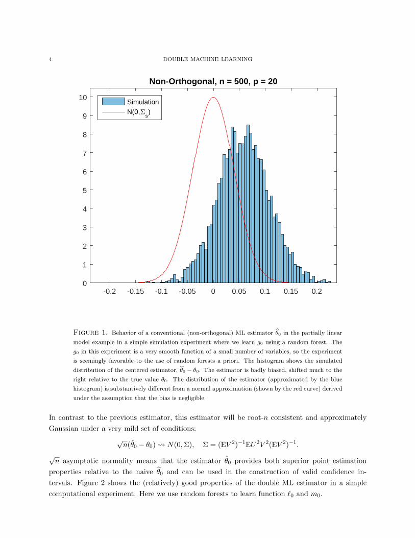
As we explain this below, the driving force behind this “inferior” behavior is the bias in learn-

ing g0(Z). Figure 1 provides a numerical illustration of this phenomenon for a conventional ML

estimator based on a random forest in a simple computational experiment.

1We consider the case where D is a scalar for simplicity; extension to the case where D is a vector of fixed, finite

dimension is accomplished by introducing an equation like (1.2) for each element of the vector.2For instance, we could use iterative methods that alternate between the random forest to find an estimator for

g0 and least squares to find an estimator for θ0.

DOUBLE MACHINE LEARNING 3

We can decompose the scaled estimation error as

√n(θ0 − θ0) =

( 1

n

n∑i=1

D2i

)−1 1√n

n∑i=1

DiUi︸︷︷︸:=a

+( 1

n

n∑i=1

D2i

)−1 1√n

n∑i=1

Di(g0(Zi)− g0(Zi))︸︷︷︸:=b

.

The first term is well-behaved under mild conditions, obeying

a N(0, Σ), Σ = (ED2)−1EU2D2(ED2)−1.

The term b is not centered however and will in general diverge:

|b| →P ∞.

Heuristically, b is the sum of n non-centered terms divided by√n, where each term contains the

estimation error g0(Zi) − g0(Zi). Thus, we expect b to be of stochastic order√nn−ϕ, where n−ϕ

is the rate of convergence of g to g0 in the root mean squared error sense and where we will have

ϕ < 1/2 in the nonparametric case. More precisely, we can use that we are using an auxiliary

sample to estimate g0 to approximate the b up to a vanishing term by

b′ = (ED2)−1 1√n

n∑i=1

m0(Zi)Bg(Zi),

where Bg(z) = g0(z)− Eg0(z) is the bias for estimating g0(z) for z in the support of Z. In typical

scenarios, the use of regularization forces the order of the squared bias to be balanced with the

variance to achieve an optimal root-mean square rate. The rate can not be faster than 1/√n

and will often be of order n−ϕ for 0 < ϕ < 1/2.3These rates mean that generically the term b′

diverges, |b′| → ∞, since E[|b′|] &√nn−ϕ →∞. The estimator θ0 will thus have an “inferior” rate

of convergence, diverging when scaled by√n, as claimed in (1.4).

Now consider a second construction that employs an “orthogonalized” formulation obtained by

directly partialing out the effect of Z from both Y and D. Specifically consider the regression

model implied by the partially linear model (1.1)-(1.2):

W = V θ0 + U,

where V = D−m0(Z) and W = Y − `0(Z), where `0(Z) = E[Y |Z] = m0(Z)θ0 + g0(Z). Regression

functions `0 and m0 can easily be directly estimated using supervised ML methods. Specifically, we

can construct 0 and m0, using an auxiliary sample, use these estimators to form W = Y − 0(Z)

and V = V − m0(Z), and then obtain an “orthogonalized” or “double ML” estimator

θ0 =( 1

n

n∑i=1

V 2i

)−1 1

n

N∑i=1

ViWi. (1.5)

3In some cases, it is possible to give up on the optimal rate of convergence for the estimator g0 and use under-

smoothing. That is, bias squared and variance are not balanced, and the order of the bias is set to o(n−1/2) which

makes b′ negligible. However, under-smoothing is typically possible only in classical low-dimensional settings.


-0.2 -0.15 -0.1 -0.05 0 0.05 0.1 0.15 0.20

1

2

3

4

5

6

7

8

9

10

Non-Orthogonal, n = 500, p = 20

SimulationN(0,'

s)

Figure 1. Behavior of a conventional (non-orthogonal) ML estimator θ0 in the partially linear

model example in a simple simulation experiment where we learn g0 using a random forest. The

g0 in this experiment is a very smooth function of a small number of variables, so the experiment

is seemingly favorable to the use of random forests a priori. The histogram shows the simulated

distribution of the centered estimator, θ0 − θ0. The estimator is badly biased, shifted much to the

right relative to the true value θ0. The distribution of the estimator (approximated by the blue

histogram) is substantively different from a normal approximation (shown by the red curve) derived

under the assumption that the bias is negligible.

In contrast to the previous estimator, this estimator will be root-n consistent and approximately

Gaussian under a very mild set of conditions:

√n(θ0 − θ0) N(0,Σ), Σ = (EV 2)−1EU2V 2(EV 2)−1.

√n asymptotic normality means that the estimator θ0 provides both superior point estimation

properties relative to the naive θ0 and can be used in the construction of valid confidence in-

tervals. Figure 2 shows the (relatively) good properties of the double ML estimator in a simple

computational experiment. Here we use random forests to learn function `0 and m0.


-0.2 -0.15 -0.1 -0.05 0 0.05 0.1 0.15 0.20

1

2

3

4

5

6

7

8

9

10

Orthogonal, n = 500, p = 20

SimulationN(0,'

s)

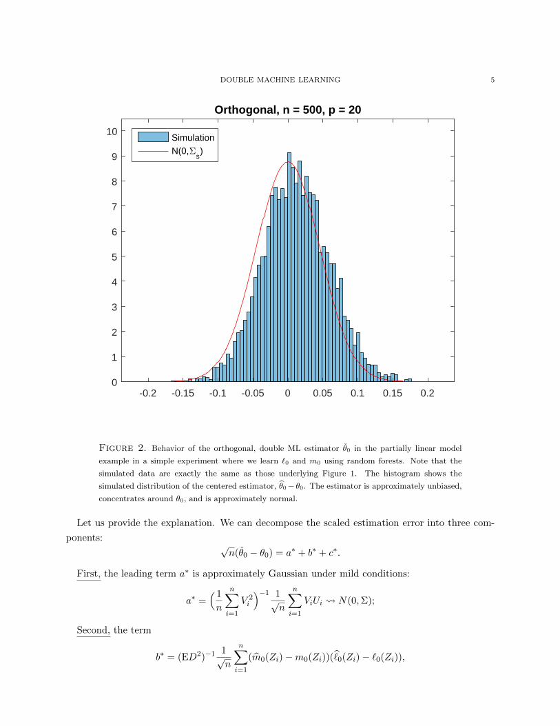
Figure 2. Behavior of the orthogonal, double ML estimator θ0 in the partially linear model

example in a simple experiment where we learn `0 and m0 using random forests. Note that the

simulated data are exactly the same as those underlying Figure 1. The histogram shows the

simulated distribution of the centered estimator, θ0− θ0. The estimator is approximately unbiased,

concentrates around θ0, and is approximately normal.

Let us provide the explanation. We can decompose the scaled estimation error into three com-

ponents:√n(θ0 − θ0) = a∗ + b∗ + c∗.

First, the leading term a∗ is approximately Gaussian under mild conditions:

a∗ =( 1

n

n∑i=1

V 2i

)−1 1√n

n∑i=1

ViUi N(0,Σ);

Second, the term

b∗ = (ED2)−1 1√n

n∑i=1

(m0(Zi)−m0(Zi))(0(Zi)− `0(Zi)),


now depends on the product of estimation errors, and so can vanish under a broad range of data-

generating processes; for example, when m0 and 0 are consistent for m0 and `0 at the o(n−1/4)

rate. Indeed, heuristically this term can be upper-bounded by√nn−(ϕm+ϕ`), where n−ϕm and n−ϕ`

are the rates of convergence of m0 to m0 and 0 to `0. It is often possible to have ϕm + ϕl > 1/2,

for example, it suffices to have ϕm > 1/4 and ϕ` > 1/4, as mentioned above. A more exact analysis

is possible when we use different parts of the auxiliary sample to estimate m0 and `0. In this case

b∗ can be approximated by

(ED2)−1 1√n

n∑i=1

Bg(Zi)B`(Zi),

where B`(z) = `0(z) − E0(z) is the bias for estimating `0(z) and Bm(z) = m0(z) − Em0(z) is

the bias for estimating m(z). If the L2(P ) norms of the biases are of order o(n−1/4), which is an

attainable rate in a wide variety of cases, then

E|c∗| 6√n√

EB2m(Z)EB2

` (Z) 6√no(n−1/2)→ 0.

Third, the term c∗ is the remainder term, which obeys

c∗ = oP (1)

and sample splitting plays a key role in driving this term to zero. Indeed, c∗ contains expressions

like ( 1

n

n∑i=1

V 2i

)−1 1√n

n∑i=1

Vi(g0(Zi)− g0(Zi)).

If we use sample splitting, conditional on the auxiliary sample, the key part of c∗, 1√n

∑ni=1 Vi(g0(Zi)−

g0(Zi)) has mean zero and variance

(EV 2)En(g0(Zi)− g0(Zi))2 → 0,

so that c∗ = oP (1). If we do not use sample splitting, the key part is bounded by

supg∈Gn

∣∣∣ 1√n

n∑i=1

Vi(g(Zi)− g0(Zi))∣∣∣,

where Gn is the smallest class of functions that contains the estimator g with high probability. The

function classes Gn are not Donsker and their entropy is growing with n, making it difficult to show

that the term in the display above vanishes. Nonetheless, if Gn’s entropy does not increase with n

too rapidly, Belloni et al. [12] have proven that the terms like the one above and c∗ more generally

do vanish. However, verification of the entropy condition is so far only available for certain classes

of machine learning methods, such as Lasso and Post-Lasso, and is likely to be difficult for practical

versions of the methods that often employ data-driven tuning and cross-validation. It is also likely

to be difficult for various hybrid methods, for example, the hybrid where we fit Random Forest

after taking out the “smooth trend” in the data by Lasso.


Now we turn to a generalization of the orthogonalization principle above. The first “conventional”

estimator θ0 given in (1.3) can be viewed as a solution for estimating equations

1

n

n∑i=1

ϕ(W, θ0, g0) = 0,

where ϕ is a known “score” function and g0 is the estimator of the nuisance parameter g0. In

the partially linear model above, the score function is ϕ(W, θ, g) = (Y − θD − g(Z))D. It is easy

to see that this score function ϕ is sensitive to biased estimation of g. Specifically, the Gateauax

derivative operator with respect to g does not vanish:

∂gEϕ(W, θ0, g)∣∣∣g=g0

6= 0.

The proofs of the general results in the next section show that this term’s vanishing is a key to

establishing good behavior of an estimator for θ0.

By contrast the orthogonalized or double ML estimator θ0 given in (1.5) solves

1

n

n∑i=1

ψ(W, θ0, η0) = 0.

where ψ is the orthogonalized or debiased “score” function and η0 is the estimator of the nuisance

parameter η0. In the partially linear model (1.1)-(1.2), the estimator uses the score function

ψ(W, θ, η) = ((Y − `(Z)−θ(D−m(Z)))(D−m(Z)), with the nuisance parameter being η = (`,m).

It is easy to see that these score functions ψ are not sensitive to biased estimation of η0. Specifically,

the Gateuax derivative operator with respect to η vanishes in this case:

∂ηEψ(W, θ0, η)∣∣∣η=η0

= 0.

The proofs of the general results in the next section show that this property is the key to generating

estimators with desired properties.

The basic problem outlined above is clearly related to the traditional semiparametric estima-

tion framework which focuses on obtaining√n-consistent and asymptotically normal estimates for

low-dimensional components with nuisance parameters estimated by conventional nonparametric

estimators such as kernels or series. See, for example, the important work by [14], [50], [40], [54],

[2], [41], [49], [38], [15], [19], [53], and [1]. The major point of departure from the present work and

this traditional work is that we allow for the use of modern ML methods, a.k.a. machine learning

methods, for modeling and fitting the non-parametric (or high-dimensional) components of the

model for modern, high-dimensional data. As noted above, considering ML estimators requires us

to accommodate estimators whose realizations belong to function classes Gn that are not Donsker

and have entropy that grows with n. Conditions employed in the traditional semiparametric liter-

ature rule out this setting which necessitates the use of a different set of tools and development of

new results. The framework we consider based on modern ML methods also expressly allows for

data-driven choice of an approximating model for the high-dimensional component which addresses

a crucial problem that arises in empirical work.


We organize there rest of the paper as follows. In Section 2, we present general theory for

orthogonalized or “double” ML estimators. We present a formal application of the general results to

estimation of average treatment effects (ATE) in partially linear model and in a fully heterogeneous

effect model in Section 3. In Section 4 we present a sample application where we apply double ML

methods to study the impact of 401(k) eligibility on accumulated assets. In an appendix, we define

some additional notation and present proofs.

Notation. The symbols P and E denote probability and expectation operators with respect to

a generic probability measure. If we need to signify the dependence on a probability measure P ,

we use P as a subscript in PP and EP . Note also that we use capital letters such as W to denote

random elements and use the corresponding lower case letters such as w to denote fixed values that

these random elements can take. In what follows, we use ‖ · ‖P,q to denote the Lq(P ) norm; for

example, we denote

‖f(W )‖P,q :=

(∫|f(w)|qdP (w)

)1/q

.

For a differentiable map x 7→ f(x), mapping Rd to Rk, we use ∂x′f to abbreviate the partial

derivatives (∂/∂x′)f , and we correspondingly use the expression ∂x′f(x0) to mean ∂x′f(x) |x=x0 ,

etc. We use x′ to denote the transpose of a column vector x.

2. A General Approach to Post-Regularized Estimation and Inference Based on

Orthogonalized Estimating Equations

2.1. Generic Construction of Orthogonal (Double ML) Estimators and Confidence Re-

gions. Here we formally introduce the model and state main results under high-level conditions.

We are interested in the true value θ0 of the low-dimensional target (causal) parameter θ ∈ Θ,

where Θ is a convex subset of Rdθ . We assume that θ0 satisfies the moment conditions

EP [ψj(W, θ0, η0)] = 0, j = 1, . . . , dθ, (2.1)

where ψ = (ψ1, . . . , ψdθ)′ is a vector of known score functions, W is a random element taking values

in a measurable space (W,AW) with law determined by a probability measure P ∈ Pn, and η0

is the true value of the nuisance parameter η ∈ T for some convex set T equipped with a norm

‖ · ‖e. We assume that the score functions ψj : W × Θ × T → R are measurable once we equip Θ

and T with their Borel σ-fields. We assume that a random sample (Wi)Ni=1 from the distribution

of W is available for estimation and inference. As explained below in detail, we employ sample-

splitting and assume that n observations are used to estimate θ0 and the other N − n observations

are used to estimate η0. The set of probability measures Pn is allowed to depend on n and in

particular to expand as n gets large. Note that our formulation allows the nuisance parameter η to

be infinite-dimensional; that is, η can be a function or a vector of functions.


As discussed in the introduction, we require the following orthogonality condition for the score

ψ. If we start with a model with score ϕ that does not satisfy this orthogonality condition, we first

transform it into a score ψ that satisfies this condition as described in the next section.

Definition 2.1 (Neyman orthogonality or unbiasedness condition). The score ψ = (ψ1, . . . , ψdθ)′

obeys the orthogonality condition with respect to T ⊂ T if the following conditions hold: The

Gateaux derivative map

Dr,j [η − η0] := ∂r

{EP

[ψj(W, θ0, η0 + r(η − η0))

]}exists for all r ∈ [0, 1), η ∈ T , and j = 1, . . . , dθ and vanishes at r = 0; namely, for all η ∈ T and

j = 1, . . . , dθ,

∂ηEPψj(W, θ0, η)∣∣∣η=η0

[η − η0] := D0,j [η − η0] = 0. (2.2)

Estimation will be carried out using the finite-sample analog of the estimating equations (2.1).

We assume that the true value η0 of the nuisance parameter η can be estimated by η0 using a part of

the data (Wi)Ni=1. Different structured assumptions on T allow us to use different machine-learning

tools for estimating η0. For instance,

1) smoothness of η0 calls for the use of adaptive kernel estimators with bandwidth values

obtained, for example, using the Lepski method;

2) approximate sparsity for η0 with respect to some dictionary calls for the use of forward

selection, lasso, post-lasso, or some other sparsity-based technique;

3) well-approximability of η0 by trees calls for the use of regression trees and random forests.

Sample Splitting

In order to set up estimation and inference, we use sample splitting. We assume that n obser-

vations with indices i ∈ I ⊂ {1, . . . , N} are used for estimation of the target parameter θ, and

the other πn = N − n observations with indices i ∈ Ic are used to provide estimator

η0 = η0(Ic)

of the true value η0 of the nuisance parameter η. The parameter π = πn determines the portion

of the entire data that is used for estimation of the nuisance parameter η. We assume that π is

bounded away from zero, that is, π > π0 > 0 for some fixed constant π0, so that πn is at least

of the same order as n, though we could allow for π → 0 as N → ∞ in principle. We assume

that I and Ic form a random partition of the set {1, ..., N}. We conduct asymptotic analysis

with respect to n increasing to ∞.

We let En, and when needed En,I , denote the empirical expectation with respect to the sample

(Wi)i∈I :

Enψ(W ) := En,I [ψ(W )] =1

n

∑i∈I

ψ(Wi).


Generic Estimation

The true value η0 of the nuisance parameter η is estimated by η0 = η0(Ic) using the sample

(Wi)i∈Ic . The true value θ0 of the target parameter θ is estimated by

θ0 = θ0(I, Ic)

using the sample (Wi)i∈I . We construct the estimator θ0 of θ0 as an approximate εn-solution

in Θ to a sample analog of the moment conditions (2.1), that is,∥∥∥En,I [ψ(W, θ0, η0)∥∥∥ 6 inf

θ∈Θ

∥∥∥En,I [ψ(W, θ, η0)]∥∥∥+ εn, εn = o(δnn

−1/2), (2.3)

where (δn)n>1 is some sequence of positive constants converging to zero.

Let ω, c0, and C0 be some strictly positive (and finite) constants, and let n0 > 3 be some positive

integer. Also, let (B1n)n>1 and (B2n)n>1 be some sequences of positive constants, possibly growing

to infinity, where B1n > 1 and B2n > 1 for all n > 1. Denote

J0 := ∂θ′{

EP [ψ(W, θ, η0)]}∣∣∣θ=θ0

. (2.4)

The quantity J0 measures the degree of identifiability of θ0 by the moment conditions (2.1). In

typical cases, the singular values of J0 will be bounded from above and away from zero.

We are now ready to state our main regularity conditions.

Assumption 2.1 (Moment condition problem). For all n > n0 and P ∈ Pn, the following

conditions hold. (i) The true parameter value θ0 obeys (2.1), and Θ contains a ball of radius

C0n−1/2 log n centered at θ0. (ii) The map (θ, η) 7→ EP [ψ(W, θ, η)] is twice continuously Gateaux-

differentiable on Θ×T . (iii) The score ψ obeys the near orthogonality condition given in Definition

2.1 for the set T ⊂ T . (iv) For all θ ∈ Θ, we have ‖EP [ψ(W, θ, η0)]‖ > 2−1‖J0(θ− θ0)‖ ∧ c0, where

singular values of J0 are between c0 and C0. (v) For all r ∈ [0, 1), θ ∈ Θ, and η ∈ T ,

(a) EP [‖ψ(W, θ, η)− ψ(W, θ0, η0)‖2] 6 C0(‖θ − θ0‖ ∨ ‖η − η0‖e)ω,

(b) ‖∂rEP [ψ(W, θ, η0 + r(η − η0))] ‖ 6 B1n‖η − η0‖e,(c) ‖∂2

rEP [ψ(W, θ0 + r(θ − θ0), η0 + r(η − η0))]‖ 6 B2n(‖θ − θ0‖2 ∨ ‖η − η0‖2e).

Assumption 2.1 is mild and standard in moment condition problems. Assumption 2.1(i) requires

θ0 to be sufficiently separated from the boundary of Θ. Assumption 2.1(ii) is rather weak because

it only requires differentiability of the function (θ, η) 7→ EP [ψ(W, θ, η)] and does not require differ-

entiability of the function (θ, η) 7→ ψ(W, θ, η). Assumption 2.1(iii) is discussed above. Assumption

2.1(iv) implies sufficient identifiability of θ0. Assumptions 2.1(v) is a smoothness condition.

Next, we state conditions related to the estimator η0. Let (∆n)n>1 and (τπn)n>1 be some se-

quences of positive constants converging to zero. Also, let a > 1, v > 0, K > 0, and q > 2 be some

constants.


Assumption 2.2 (Quality of estimation of nuisance parameter and score regularity).

For all n > n0 and P ∈ Pn, the following conditions hold. (i) With probability at least 1−∆n, we

have η0 ∈ T . (ii) For all η ∈ T , we have ‖η − η0‖e 6 τπn. (iii) The true value η0 of the nuisance

parameter η satisfies η0 ∈ T . (iv) For all η ∈ T , the function class F1,η = {ψj(·, θ, η) : j =

1, ..., dθ, θ ∈ Θ} is suitably measurable and its uniform entropy numbers obey

supQ

logN(ε‖F1,η‖Q,2,F1,η, ‖ · ‖Q,2) 6 v log(a/ε), for all 0 < ε 6 1 (2.5)

where F1,η is a measurable envelope for F1,η that satisfies ‖F1,η‖P,q 6 K. (v) For all η ∈ T and

f ∈ F1,η, we have c0 6 ‖f‖P,2 6 C0. (vi) The estimation rate τπn satisfies (a) n−1/2 6 C0τπn, (b)

(B1nτπn)ω/2 + n−1/2+1/q 6 C0δn, and (c) n1/2B21nB2nτ

2πn 6 C0δn.

Assumption 2.2 states requirements on the quality of estimation of η0 as well as imposes some

mild assumptions on the score ψ. The estimator η0 has to converge to η0 at the rate τπn, which

needs to be faster than n−1/4, with a more precise requirement stated above. Note that if π → 0,

the requirements on the quality of η0 become more stringent. This rate condition is widely used

in traditional semi-parametric estimation which employs classical nonparametric estimators for η0.

The new generation of machine learning methods are often able to perform much better than the

classical methods, and so the requirement may be more easily satisfied by these methods. Suitable

measurability, required in Assumption 2.2(iv), is a mild regularity condition that is satisfied in all

practical cases. Assumption 2.2(vi) is a set of growth conditions.

Theorem 2.1 (Uniform Bahadur Representation and Approximate Normality). Under

Assumptions 2.1 and 2.2, the estimator θ0 defined by equation (2.3), obeys

√nΣ−1/20 (θ0 − θ0) =

1√n

∑i∈I

ψ(Wi) +OP (δn) N(0, I),

uniformly over P ∈ Pn, where ψ(·) := −Σ−1/20 J−1

0 ψ(·, θ0, η0) and

Σ0 := J−10 EP [ψ(W, θ0, η0)ψ(W, θ0, η0)′](J−1

0 )′.

The result establishes that the estimator based on the orthogonalized scores achieves the root-n

rate of convergence and is approximately normally distributed. It is noteworthy that this conver-

gence result, both rate and distributional approximation, holds uniformly with respect to P varying

over an expanding class of probability measures Pn. This means that the convergence holds under

any sequence of probability distributions {Pn} with Pn ∈ Pn for each n, which in turn implies that

the results are robust with respect to perturbations of a given P along such sequences. The same

property can be shown to fail for methods not based on orthogonal scores. The result can be used

for standard construction of confidence regions which are uniformly valid over a large, interesting

class of models.

An estimator based on sample-splitting does not use the full sample by construction. However,

there will be no asymptotic loss in efficiency from sample splitting if it is possible to send πn ↘ 0


while satisfying Assumption 2.1. Such a sequence requires the number of observations πnn used

for producing η0 to be small compared to n while also requiring the estimator of the nuisance

parameter to remain of sufficient quality given this small number of observations.

Corollary 2.1 (Achieving no efficiency loss from sample-splitting). (1) If πn → 0 and the

conditions of Theorem 2.1 continue to hold, the sample-splitting estimator obeys

√NΣ

−1/20 (θ0 − θ0) =

1√N

N∑i=1

ψ(Wi) + oP (1) N(0, I),

uniformly over P ∈ Pn. That is, it is as asymptotically efficient as using all N observations.

Below we explore alternative ways of sample splitting.

2.2. Achieving Full Efficiency by Cross-Fitting. Here we exploit the use of cross-fitting, fol-

lowing [3], for preventing loss of efficiency.

Full Efficiency by 2-fold Cross-Fitting

We could proceed with a random 50-50 split of {1, ..., N} into I and Ic. This means that the

ratio of the sizes of the samples Ic and I is π = 1. Indeed, the size of I is n, the size of Ic

is also n, and the total sample size is N = 2n. We may then construct an estimator θ0(I, Ic)

that employs the nuisance parameter estimator η0(Ic), as before. Then, we reverse the roles of

I and Ic and construct an estimator θ0(Ic, I) that employs the nuisance parameter estimator

η0(I). The two estimators may then be aggregated into the final estimator:

θ0 = θ0(I, Ic)/2 + θ(I, Ic)/2. (2.6)

This 2-fold cross-fitting generalizes to the K-fold cross-fitting, which is subtly different from

(and hence should not be confused with) cross-validation. This approach can be thought as a

“leave-a-block out” approach.

Full Efficiency by K-fold Cross-Fitting

We could proceed with a K-fold random split Ik, k = 1, ...,K of the entire sample {1, ..., N}, so

that π = K − 1. In this case, the size of each split Ik is n = N/K, the size of Ick = ∪m6=kIm is

N · [(K − 1)/K], and the total sample size is N . We may then construct K estimators

θ0(Ik, Ick), k = 1, ...,K,

that employ the nuisance parameter estimators η0(Ick). The K estimators may then be aggre-

gated into

θ0 =1

K

K∑k=1

θ0(Ik, Ick). (2.7)


The following is an immediate corollary of Theorem 2.1 that shows that resulting estimators

entail no loss from sample-splitting asymptotically under assumptions of the theorem.

Theorem 2.2 (Achieving no efficiency loss by K-fold cross-fitting). Under the conditions

of Theorem 2.1, the aggregated estimator θ0 defined by equation (2.7), obeys

√NΣ

−1/20 (θ0 − θ0) =

1√N

N∑i=1

ψ(Wi) + oP (1) N(0, I),

uniformly over P ∈ Pn.

If the score function turns out to be efficient for estimating θ0, then the resulting estimator is

also efficient in the semi-parametric sense.

Corollary 2.2 (Semi-parametric efficiency). If the score function ψ is the efficient score for

estimating θ0 at a given P ∈ P ⊂ Pn, in the semi-parametric sense as defined in [55], then the

large sample variance Σ of θ0 reaches the semi-parametric efficiency bound at this P relative to the

model P.

Note that efficient scores are automatically orthogonal with respect to the nuisance parameters

by construction as discussed below. It should be noted though that orthogonal scores do not have

to be efficient scores. For instance, the scores discussed in the introduction for the partially linear

are only efficient in the homoscedastic model.

2.3. Construction of score functions satisfying the orthogonality condition. Here we dis-

cuss several methods for generating orthogonal scores in a wide variety of settings, including the

classical Neyman’s construction.

1) Orthogonal Scores for Likelihood Problems with Finite-Dimensional Nuisance Pa-

rameters. In likelihood settings with finite-dimensional parameters, the construction of orthogonal

equations was proposed by Neyman [42] who used them in construction of his celebrated C(α)-

statistic.4

Suppose that the log-likelihood function associated to observation W is (θ, β) 7→ `(W, θ, β), where

θ ∈ Θ ⊂ Rd is the target parameter and β ∈ T ⊂ Rp0 is the nuisance parameter. Under regularity

conditions, the true parameter values θ0 and β0 obey

E[∂θ`(W, θ0, β0)] = 0, E[∂β`(W, θ0, β0)] = 0. (2.8)

Note that the original score function ϕ(W, θ, β) = ∂θ`(W, θ, β) in general does not possess the

orthogonality property. Now consider the new score function

ψ(W, θ, η) = ∂θ`(W, θ, β)− µ∂β`(W, θ, β), (2.9)

4The C(α)-statistic, or the orthogonal score statistic, has been explicitly used for testing and estimation in high-

dimensional sparse models in [10]. The discussion of Neyman’s construction here draws on [28].


where the nuisance parameter is

η = (β′, vec(µ)′)′ ∈ T ×D ⊂ Rp, p = p0 + dp0,

µ is the d× p0 orthogonalization parameter matrix whose true value µ0 solves the equation

Jθβ − µJββ = 0 (i.e., µ0 = JθβJ−1ββ ),

and

J =

(Jθθ Jθβ

Jβθ Jββ

)= ∂(θ′,β′)E

[∂(θ′,β′)′`(W, θ, β)

]∣∣∣θ=θ0; β=β0

.

Provided that µ0 is well-defined, we have by (2.8) that

E[ψ(W, θ0, η0)] = 0,

where η0 = (β′0, vec(µ0)′)′. Moreover, it is trivial to verify that under standard regularity conditions

the score function ψ obeys the orthogonality condition (2.2) exactly, that is,

∂ηE[ψ(W, θ0, η)]∣∣∣η=η0

= 0.

Note that in this example, µ0 not only creates the necessary orthogonality but also creates the

efficient score for inference on the target parameter θ, as emphasized by Neyman [42].

2) Orthogonal Scores for Likelihood Problems with Infinite-Dimensional Nuisance Pa-

rameters. Neyman’s construction can be extended to semi-parametric models where the nuisance

parameter β is a function. In this case, the original score functions (θ, β) 7→ ∂θ`(W, θ, β) corre-

sponding to the log-likelihood function (θ, β) 7→ `(W, θ, β) associated to observation W can be

transformed into efficient score functions ψ that obey the orthogonality condition by projecting the

original score functions onto the orthocomplement of the tangent space induced by the nuisance

parameter β; see Chapter 25 of [55] for a detailed description of this construction. By selecting

elements of the orthocomplement, we generate scores that are orthogonal but not necessarily effi-

cient. The projection gives the unique score that is efficient. Note that the projection may create

additional nuisance parameters, so that the new nuisance parameter η could be of larger dimen-

sion than β. Other relevant references include [56], [33], [8], and [10]. The approach is related to

Neyman’s construction in the sense that the score ψ arising in this model is actually the Neyman’s

score arising in a one-dimensional least favorable parametric subfamily; see Chapter 25 of [55] for

details.

3) Orthogonal Scores for Conditional Moment Problems with Infinite-Dimensional

Nuisance Parameters. Next, consider a conditional moment restrictions framework studied by

Chamberlain [18]:

E[ϕ(W, θ0, h0(X)) | X] = 0,

where X and W are random vectors with X being a sub-vector of W , θ ∈ Θ ⊂ Rd is a finite-

dimensional parameter whose true value θ0 is of interest, h is a functional nuisance parameter


mapping the support of X into a convex set V ⊂ Rl whose true value is h0, and ϕ is a known

function with values in Rk for k > d + l. This framework is of interest because it covers a rich

variety of models without having to explicitly rely on the likelihood formulation.

Here we would like to build a (generalized) score function (θ, η) 7→ ψ(W, θ, η) for estimating θ0,

the true value of parameter θ, where η is a new nuisance parameter with true value η0 that obeys

the orthogonality condition (2.2). To this end, let v 7→ E[ϕ(W, θ0, v) | X] be a function mapping

Rl into Rk and let

γ(X, θ0, h0) = ∂v′E[ϕ(W, θ0, v) | X]|v=h0(X)

be a k × l matrix of its derivatives. We will set η = (h, β,Σ) where β is a function mapping the

support of X into the space of d× k matrices, Rd×k, and Σ is the function mapping the support of

X into the space of k × k matrices, Rk×k. Define the true value β0 of β as

β0(X) = A(X)(Ik×k −Π(X)),

where A(X) is a d×k matrix of measurable transformations of X, Ik×k is the k×k identity matrix,

and Π(X) 6= Ik×k is a k × k non-identity matrix with the property:

Π(X)Σ−1/20 (X)γ(X, θ0, h0) = Σ

−1/20 (X)γ(X, θ0, h0), (2.10)

where Σ0 is the true value of parameter Σ. For example, Π(X) can be chosen to be an orthogonal

projection matrix:

Π(X) =[Σ0(X)−1/2γ(X, θ0, h0)

(γ(X, θ0, h0)′Σ0(X)−1γ(X, θ0, h0)

)−1

× γ(X, θ0, h0)′Σ0(X)−1/2].

Then an orthogonal score for the problem above can be constructed as

ψ(W, θ, η) = β(X)Σ−1/2(X)ϕ(Z, θ, h(X)), η = (h, β,Σ).

It is straightforward to check that under mild regularity conditions the score function ψ satis-

fies E[ψ(W, θ0, η0)] = 0 for η0 = (h0, ϕ0,Σ0) and also obeys the exact orthogonality condition.

Furthermore, by setting

A(X) =(∂θ′E[ϕ(W, θ, h0(X) | X]|θ=θ0

)′, Σ0(X) = E

[ϕ(W, θ0, h0(X))ϕ(W, θ0, h0(X))′|X

],

and using Π(X) suggested above, we obtain the efficient score ψ that yields an estimator of θ0

achieving the semi-parametric efficiency bound, as calculated by Chamberlain [18].

3. Application to Estimation of Treatment Effects

3.1. Treatment Effects in the Partially Linear Model. Here we revisit the partially linear

model

Y = Dθ0 + g0(Z) + ζ, E[ζ | Z,D] = 0, (3.1)

D = m0(Z) + V, E[V | Z] = 0. (3.2)


If D is as good as randomly assigned conditional on covariates, then θ0 measures the average

treatment effect of D on potential outcomes.

The first approach, which we described in the introduction, employs the score function

ψ(W, θ, η) := {Y − `(Z)− θ(D −m(Z))}(D −m(Z)), η = (`,m), (3.3)

where ` and m are P -square-integrable functions mapping the support of Z to R.

It is easy to see that θ0 is a solution to

EPψ(W, θ0, η0) = 0,

and the orthogonality condition holds:

∂ηEPψ(W, θ0, η)∣∣∣η=η0

= 0, η0 = (`0,m0),

where `0(Z) = EP [Y |Z]. This approach represents a generalization of the approach of [7, 8]

considered for the case of Lasso without cross-fitting. As mentioned, this generalization opens up

the use of a much broader collection of machine learning methods, much beyond Lasso.

The second approach, which is first-order equivalent to the first, is to employ the score function

ψ(W, θ, η) := {Y −Dθ − g(Z)}(D −m(Z)), η = (g,m), (3.4)

where g and m are P -square-integrable functions mapping the support of Z to R. It is easy to see

that θ0 is a solution to

EPψ(W, θ0, η0) = 0,

and the orthogonality condition holds:


= 0, η0 = (g0,m0).

This approach can be seen as “debiasing” the score function (Y − Dθ − g(Z))D, which does not

possess the orthogonality property unless m0(Z) = 0. This second approach represents a gener-

alization of the approach of [31, 52, 57] considered for the case of Lasso-type methods without

cross-fitting. Like above, our generalization allows for the use of broad collection machine learning

methods, much beyond Lasso-type methods.

Algorithm 1 (Double ML Estimation and Inference on ATE in the Partially Linear

Model.). We describe two estimators of θ0 based on the use of score functions (3.3) and (3.3).

Let K be a fixed integer. We construct a K-fold random partition of the entire sample {1, ..., N}into equal parts (Ik)

Kk=1 each of size n := N/K, and construct the K estimators

θ0(Ik, Ick), k = 1, ...,K,

where each estimator θ0(Ik, Ick) is the root θ of the equation:

1

n

∑i∈Ik

ψ(W, θ, η0(Ick)) = 0,


for the score ψ defined in (3.3) or (3.4); for the case with the score function given by (3.3), the

estimator employs the nuisance parameter estimators

η0(Ick) := (0(Z; Ick), m0(Z; Ick)),

based upon machine learning estimators of `0(Z) and m0(Z) using auxiliary sample Ick; and, for

the case with the score function given by (3.4), the estimator employs the nuisance parameter

estimators

η0(Ick) := (g0(Z; Ick), m0(Z; Ick)),

based upon machine learning estimators of g0(Z) and m0(Z) using auxiliary sample Ick.

We then average the K estimators to obtain the final estimator:

θ0 =1

K

K∑k=1

θ0(Ik, Ick). (3.5)

The approximate standard error for this estimator is given by σ/√N , where

σ2 =( 1

N

N∑i=1

V 2i

)−2 1

N

N∑i=1

V 2i ζ

2i ,

where Vi := Di − m(Zi, Ick(i)), ζi := (Yi − 0(Zi, I

ck(i)) − (Di − m0(Z0, I

ck(i)))θ0 or ζi := Yi −

Diθ0 − g0(Z0, Ick(i)) , and k(i) := {k ∈ {1, ...,K} : i ∈ Ik}. The approximate (1 − α) × 100%

confidence interval is given by:

[θ0 ± Φ−1(1− α/2)σ/√N ].

Let (δn)∞n=1 and (∆n)∞n=1 be sequences of positive constants approaching 0 as before. Let c and

C be fixed positive constants and K > 2 be a fixed integer, and let q > 4.

Assumption 3.1. Let P be the collection of probability laws P for the triple (Y,D,Z) such that: (i)

equations (3.1)-(3.2) hold; (ii) the true parameter value θ0 is bounded, |θ0| 6 C; (iii) ‖X‖P,q 6 C

for X ∈ {Y,D, g0(Z), `0(Z),m0(Z)}; (iv) ‖V ‖P,2 > c and ‖ζ‖P,2 > c; and (v) the ML estimators of

the nuisance parameters based upon a random subset Ick of {1, ..., N} of size N − n, for n = N/K,

obey the condition: ‖η0(Z, Ick) − η0(Z, Ick)‖P,2 6 δnn−1/4 for all n > 1 with P -probability no less

than 1−∆n.

Comment 3.1. The only non-primitive condition is the assumption on the rate of estimating the

nuisance parameters. These rates of convergence are available for most often used ML methods

and are case-specific, so we do not restate conditions that are needed to reach these rates. The

conditions are not the tightest possible, but we choose to present the simple ones, so that results

below follows as a special case of the general theorem of the previous section. We can easily obtain

more refined conditions by doing customized proofs. �


The following theorem follows as a corollary to the results in the previous section.

Theorem 3.1 (Estimation and Inference on Treatment Effects in the Partially Linear Model).

Suppose Assumption 3.1 holds. Then, as N → ∞, both of the two double ML estimators θ0,

constructed in Algorithm 1 above, are first-order equivalent and obey

σ−1√N(θ0 − θ0) N(0, 1),

uniformly over P ∈ P, where σ2 = [EPV2]−1EP [V 2ζ2][EPV

2]−1, and the result continues to hold if

σ2 is replaced by σ2. Furthermore, the confidence regions based upon Double ML estimator θ0 have

the uniform asymptotic validity:

limN→∞

supP∈P

∣∣∣PP (θ0 ∈ [θ0 ± Φ−1(1− α/2)σ/√N ])− (1− α)

∣∣∣ = 0.

Comment 3.2. Note that under conditional homoscedasticity, namely E[ζ2|Z] = E[ζ2], the as-

ymptotic variance σ2 reduces to E[V 2]−1E[ζ2], which is the semi-parametric efficiency bound for

the partially linear model. �

3.2. Treatment Effects in the Interactive Model. We next consider estimation of average

treatment effects (ATE) when treatment effects are fully heterogeneous and the treatment variable

is binary, D ∈ {0, 1}. We consider vectors (Y,D,Z) such that

Y = g0(D,Z) + ζ, E[ζ | Z,D] = 0, (3.6)

D = m0(Z) + ν, E[ν | Z] = 0. (3.7)

Since D is not additively separable, this model is more general than the partially linear model for

the case of binary D. A common target parameter of interest in this model is the average treatment

effect (ATE),

E[g0(1, Z)− g0(0, Z)].

Another common target parameter is the average treatment effect for the treated (ATTE)

E[g0(1, Z)− g0(0, Z)|D = 1].

The confounding factors Z affect the policy variable via the propensity score m(Z) and the

outcome variable via the function g0(D,Z). Both of these functions are unknown and potentially

complicated, and we can employ machine learning methods to learn them.

We proceed to set up moment conditions with scores obeying orthogonality conditions. For

estimation of the ATE, we employ

ψ(W, θ, η) := (g(1, Z)− g(0, Z)) +D(Y − g(1, Z))

m(Z)− (1−D)(Y − g(0, Z))

1−m(Z)− θ,

η(Z) := (g(0, Z), g(1, Z),m(Z)), η0(Z) := (g0(0, Z), g0(1, Z),m0(Z))′,

(3.8)


where η(Z) is the nuisance parameter consisting of P -square integrable functions mapping the

support of Z to R× R× (ε, 1− ε), with the true value of this parameter denoted by η0(Z), where

ε > 0 is a constant.

For estimation of ATTE, we use the score

ψ(W, θ, η) =D(Y − g(0, Z))

m− m(Z)(1−D)(Y − g(0, Z))

(1−m(Z))m− θD

m,

η(Z) := (g(0, Z), g(1, Z),m(Z),m), η0(Z) = (g0(0, Z), g0(1, Z),m0(Z),E[D]),′(3.9)

where η(Z) is the nuisance parameter consisting of three P -square integrable functions mapping

the support of Z to R × R × (ε, 1 − ε) and a constant m ∈ (ε, 1 − ε), with the true value of this

parameter denoted by η0(Z).

It can be easily seen that true parameter values θ0 for ATE and ATTE obey

EPψ(W, θ0, η0) = 0,

for the respective scores and that the scores have the required orthogonality property:


= 0.

Algorithm 2 (Double ML Estimation and Inference on ATE and ATTE in the

Interactive Model.). We describe the estimator of θ0 next. Let K be a fixed integer. We

construct a K-fold random partition of the entire sample {1, ..., N} into equal parts (Ik)Kk=1

each of size n := N/K, and construct the K estimators

θ0(Ik, Ick), k = 1, ...,K,

that employ the machine learning estimators

η0(Ick) =

g0(0, Z; Ick), g0(1, Z; Ick), m0(Z; Ick),1

N − n∑i∈Ick

Di

′ ,of the nuisance parameters

η0(Z) = (g0(0, Z), g0(1, Z),m0(Z),E[D]),

and where each estimator θ0(Ik, Ick) is defined as the root θ of the corresponding equation:

1

n

∑i∈Ik

ψ(W, θ, η0(Ick)) = 0,

for the score ψ defined in (3.8) for ATE and in (3.9) for ATTE.

We then average the K estimators to obtain the final estimator:

θ0 =1

K

K∑k=1

θ0(Ik, Ick). (3.10)


The approximate standard error for this estimator is given by σ/√N , where

σ2 =1

N

N∑i=1

ψ2i

where ψi := ψ(Wi, θ0, η0(Ick(i))), and k(i) := {k ∈ {1, ...,K} : i ∈ Ik}. The approximate

(1− α)× 100% confidence interval is given by

[θ0 ± Φ−1(1− α/2)σ/√N ].

Let (δn)∞n=1 and (∆n)∞n=1 be sequences of positive constants approaching 0, as before, and c, ε, C

and q > 4 be fixed positive constants, and K be a fixed integer.

Assumption 3.2 (TE in the Heterogenous Model). Let P be the set of probability distributions P

for (Y,D,Z) such that (i) equations (3.6)-(3.7) hold, with D ∈ {0, 1}, (ii) the moment conditions

hold: ‖g‖P,q 6 C, ‖Y ‖P,q 6 C, P (ε 6 m0(Z) 6 1 − ε) = 1, and ‖ζ2‖P,2 > c, and (ii) the ML

estimators of the nuisance parameters based upon a random subset Ick of {1, ..., N} of size N − n,

for n = N/K, obey the condition: ‖g0(D,Z, Ick) − g0(D,Z, Ick)‖P,2 + ‖m0(Z, Ick) −m0(Z, Ick)‖P,2 6δnn

−1/4 and ‖m0(Z, Ick)−m0(Z, Ick)‖P,∞ 6 δn, for all n > 1 with P -probability no less than 1−∆n.

Comment 3.3. The only non-primitive condition is the assumption on the rate of estimating the

nuisance parameters. These rates of convergence are available for most often used ML methods

and are case-specific, so we do not restate conditions that are needed to reach these rates. The

conditions are not the tightest possible, but we chose to present the simple ones, since the results

below follow as a special case of the general theorem of the previous section. We can easily obtain

more refined conditions by doing customized proofs. �

The following theorem follows as a corollary to the results in the previous section.

Theorem 3.2 (Double ML Inference on ATE and ATT). (1) Suppose that the ATE, θ0 =

E[g0(1, Z) − g0(0, Z)], is the target parameter and we use the estimator θ0 and other notations

defined above. (2) Alternatively, suppose that the ATTE, θ0 = E[g0(1, Z) − g0(0, Z) | D = 1], is

the target parameter and we use the estimator θ0 and other notations above. Consider the set P of

data generating defined in Assumption 3.2. Then uniformly in P ∈ P, the Double ML estimator θ0

concentrates around θ0 with the rate 1/√N and is approximately unbiased and normally distributed:

σ−1√N(θ0 − θ0) N(0, 1), σ2 = EP [ψ2(W, θ0, η0(Z))], (3.11)

uniformly over P ∈ P, and the result continues to hold if σ2 is replaced by σ2. Moreover, the

confidence regions based upon Double ML estimator θ0 have uniform asymptotic validity:

limN→∞

supP∈P

∣∣∣PP (θ0 ∈ [θ0 ± Φ−1(1− α/2)σ/√N ])− (1− α)

∣∣∣ = 0.


The scores ψ are the efficient scores, so both estimators are asymptotically efficient, reaching the

semi-parametric efficiency bound of [30].

4. Empirical Example

To illustrate the methods developed in the preceding sections, we consider the estimation of

the effect of 401(k) eligibility on accumulated assets. The key problem in determining the effect

of 401(k) eligibility is that working for a firm that offers access to a 401(k) plan is not randomly

assigned. To overcome the lack of random assignment, we follow the strategy developed in [45]

and [46]. In these papers, the authors use data from the 1991 Survey of Income and Program

Participation and argue that eligibility for enrolling in a 401(k) plan in this data can be taken as

exogenous after conditioning on a few observables of which the most important for their argument is

income. The basic idea of their argument is that, at least around the time 401(k)’s initially became

available, people were unlikely to be basing their employment decisions on whether an employer

offered a 401(k) but would instead focus on income and other aspects of the job. Following this

argument, whether one is eligible for a 401(k) may then be taken as exogenous after appropriately

conditioning on income and other control variables related to job choice.

A key component of the argument underlying the exogeneity of 401(k) eligibility is that eligibility

may only be taken as exogenous after conditioning on income and other variables related to job

choice that may correlate with whether a firm offers a 401(k). [45] and [46] and many subsequent

papers adopt this argument but control only linearly for a small number of terms. One might

wonder whether such specifications are able to adequately control for income and other related

confounds. At the same time, the power to learn about treatment effects decreases as one allows

more flexible models. The principled use of flexible machine learning tools offers one resolution

to this tension. The results presented below thus complement previous results which rely on the

assumption that confounding effects can adequately be controlled for by a small number of variables

chosen ex ante by the researcher.

In the example in this paper, we use the same data as in [27]. We use net financial assets - defined

as the sum of IRA balances, 401(k) balances, checking accounts, U.S. saving bonds, other interest-

earning accounts in banks and other financial institutions, other interest-earning assets (such as

bonds held personally), stocks, and mutual funds less non-mortgage debt - as the outcome variable,

Y , in our analysis. Our treatment variable, D, is an indicator for being eligible to enroll in a 401(k)

plan. The vector of raw covariates, Z, consists of age, income, family size, years of education, a

married indicator, a two-earner status indicator, a defined benefit pension status indicator, an IRA

participation indicator, and a home ownership indicator.

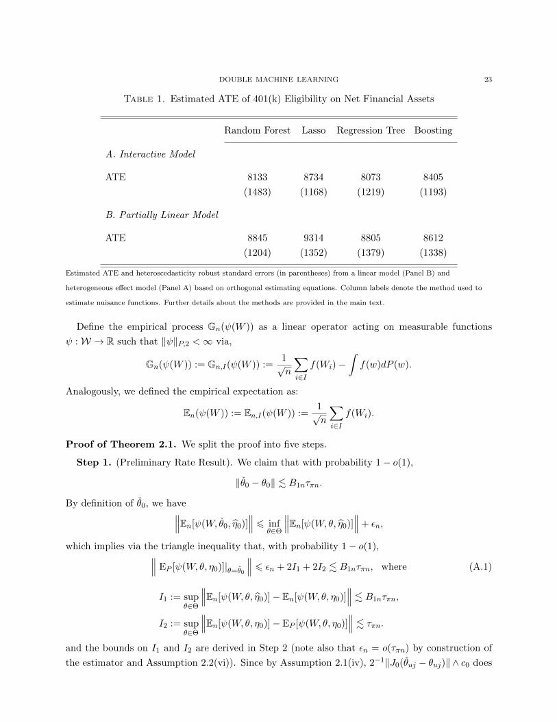
We report estimates of the average treatment effect (ATE) of 401(k) eligibility on net financial

assets both in the partially linear model as in (1.1) and allowing for heterogeneous treatment effects

using the approach outlined in Section 3.2 in Table 1. All results are based on sample-splitting as

discussed in Section 2.1 using a 50-50 split. We report results based on four different methods for


estimating the nuisance functions used in forming the orthogonal estimating equations. We consider

three tree-based methods, labeled “Random Forest”, “Regression Tree”, and “Boosting”, and one

`1-penalization based method, labeled “Lasso”. For “Regression Tree,” we fit a single CART tree

to estimate each nuisance function with penalty parameter chosen by 10-fold cross-validation. The

results in column “Random Forest” are obtained by estimating each nuisance function with a

random forest using default settings as in [17]. Results in “Boosting” are obtained using boosted

regression trees with default settings from [48]. “Lasso” results use conventional lasso regression

with penalty parameter chosen by 10-fold cross-validation to estimate conditional expectations of

net financial assets and use `1-penalized logistic regression with penalty parameter chosen by 10-

fold cross-validation when estimating conditional expectations of 401(k) eligibility. For the three

tree-based methods, we use the raw set of covariates as features. For the `1-penalization based

method, we use a set of 275 potential control variables formed from the raw set of covariates and

all second order terms, i.e. squares and first-order interactions.

Turning to the results, it is first worth noting that the estimated effect ATE of 401(k) eligibility

on net financial assets is $19,559 with an estimated standard error of 1413 when no control variables

are used. Of course, this number is not a valid estimate of the causal effect of 401(k) eligibility on

financial assets if there are neglected confounding variables as suggested by [45] and [46]. When we

turn to the estimates that flexibly account for confounding reported in Table 1, we see that they are

substantially attenuated relative to this baseline that does not account for confounding, suggesting

much smaller causal effects of 401(k) eligiblity on financial asset holdings. It is interesting and

reassuring that the results obtained from the different flexible methods are broadly consistent with

each other. This similarity is consistent with the theory that suggests that results obtained through

the use of orthogonal estimating equations and any sensible method of estimating the necessary

nuisance functions should be similar. Finally, it is interesting that these results are also broadly

consistent with those reported in the original work of [45] and [46] which used a simple intuitively

motivated functional form, suggesting that this intuitive choice was sufficiently flexible to capture

much of the confounding variation in this example.

Appendix A. Proofs

In this appendix, we use C to denote a strictly positive constant that is independent of n and

P ∈ Pn. The value of C may change at each appearance. Also, the notation an . bn means that

an 6 Cbn for all n and some C. The notation an & bn means that bn . an. Moreover, the notation

an = o(1) means that there exists a sequence (bn)n>1 of positive numbers such that (i) |an| 6 bn for

all n, (ii) bn is independent of P ∈ Pn for all n, and (iii) bn → 0 as n → ∞. Finally, the notation

an = OP (bn) means that for all ε > 0, there exists C such that PP (an > Cbn) 6 1 − ε for all n.

Using this notation allows us to avoid repeating “uniformly over P ∈ Pn” many times in the proofs.


Table 1. Estimated ATE of 401(k) Eligibility on Net Financial Assets

Random Forest Lasso Regression Tree Boosting

A. Interactive Model

ATE 8133 8734 8073 8405

(1483) (1168) (1219) (1193)

B. Partially Linear Model

ATE 8845 9314 8805 8612

(1204) (1352) (1379) (1338)

Estimated ATE and heteroscedasticity robust standard errors (in parentheses) from a linear model (Panel B) and

heterogeneous effect model (Panel A) based on orthogonal estimating equations. Column labels denote the method used to

estimate nuisance functions. Further details about the methods are provided in the main text.

Define the empirical process Gn(ψ(W )) as a linear operator acting on measurable functions

ψ :W → R such that ‖ψ‖P,2 <∞ via,

Gn(ψ(W )) := Gn,I(ψ(W )) :=1√n

∑i∈I

f(Wi)−∫f(w)dP (w).

Analogously, we defined the empirical expectation as:

En(ψ(W )) := En,I(ψ(W )) :=1√n

∑i∈I

f(Wi).

Proof of Theorem 2.1. We split the proof into five steps.

Step 1. (Preliminary Rate Result). We claim that with probability 1− o(1),

‖θ0 − θ0‖ . B1nτπn.

By definition of θ0, we have∥∥∥En[ψ(W, θ0, η0)]∥∥∥ 6 inf

θ∈Θ

∥∥∥En[ψ(W, θ, η0)]∥∥∥+ εn,

which implies via the triangle inequality that, with probability 1− o(1),∥∥∥ EP [ψ(W, θ, η0)]|θ=θ0∥∥∥ 6 εn + 2I1 + 2I2 . B1nτπn, where (A.1)

I1 := supθ∈Θ

∥∥∥En[ψ(W, θ, η0)]− En[ψ(W, θ, η0)]∥∥∥ . B1nτπn,

I2 := supθ∈Θ

∥∥∥En[ψ(W, θ, η0)]− EP [ψ(W, θ, η0)]∥∥∥ . τπn.

and the bounds on I1 and I2 are derived in Step 2 (note also that εn = o(τπn) by construction of

the estimator and Assumption 2.2(vi)). Since by Assumption 2.1(iv), 2−1‖J0(θuj − θuj)‖ ∧ c0 does


not exceed the left-hand side of (A.1), minimal singular values J0 are bounded away from zero, and

by Assumption 2.2(vi), B1nτπn = o(1), we conclude that

‖θ0 − θ0‖ . B1nτπn, (A.2)

with probability 1− o(1) yielding the claim of this step.

Step 2. (Bounds on I1 and I2) We claim that with probability 1− o(1),

I1 . B1nτπn and I2 . τπn.

To show these relations, observe that with probability 1−o(1), we have I1 6 2I1a+I1b and I2 6 I1a,

where

I1a := maxη∈{η0,η0}

supθ∈Θ

∥∥∥En[ψ(W, θ, η)]− EP [ψ(W, θ, η)]∥∥∥,

I1b := supθ∈Θ,η∈T

∥∥∥EP [ψ(W, θ, η)]− EP [ψ(W, θ, η0)]∥∥∥.

To bound I1b, we employ Taylor’s expansion:

I1b . maxj6dθ

supθ∈Θ,η∈T,r∈[0,1)

∣∣∣∂rEP [ψj(W, θ, η0 + r(η − η0))]∣∣∣ . B1n sup

η∈T‖η − η0‖e 6 B1nτπn,

by Assumptions 2.1(v) and 2.2(ii).

To bound I1a, we can apply the maximal inequality of Lemma A.1 to the function class F1,η

for η = η0 and η = η0 defined in Assumption 2.2, conditional on (Wi)i∈Ic so that η0 is fixed after

conditioning. Note that (Wi)i∈I are i.i.d. conditional on Ic. We conclude that with probability

1− o(1),

I1a . n−1/2

(1 + n−1/2+1/q

). τn. (A.3)

Combining presented bounds gives the claim of this step.

Step 3. (Linearization) Here we prove the claim of the theorem. By definition of θ0, we have

√n∥∥∥En[ψ(W, θ0, η0)]

∥∥∥ 6 infθ∈Θ

√n∥∥∥En[ψ(W, θ, η0)]

∥∥∥+ εn√n. (A.4)

Also, for any θ ∈ Θ and η ∈ T , we have

√nEn[ψ(W, θ, η)] =

√nEn[ψ(W, θ0, η0)]−Gnψ(W, θ0, η0) (A.5)

−√n(

EP [ψ(W, θ0, η0)]− EP [ψ(W, θ, η)])

+ Gnψ(W, θ, η).

Moreover, by Taylor’s expansion of the function r 7→ EP [ψ(W, θ0 + r(θ − θ0), η0 + r(η − η0))],

EP [ψ(W, θ, η)]− EP [ψ(W, θ0, η0)] (A.6)

= J0(θ − θ0) + D0[η − η0] + ∂2rEP [W, θ0 + r(θ − θ0), η0 + r(η − η0)]

∣∣r=r


for some r ∈ (0, 1), which may differ for each row of the vector in the display. Substituting this

equality into (A.5), taking θ = θ0 and η = η0, and using (A.4) gives

√n∥∥∥En[ψ(W, θ0, η0)] + J0(θ0 − θ0) + D0[η0 − η0]

∥∥∥6 εn√n+ inf

θ∈Θ

√n‖En[ψ(W, θ, η0)]‖+ II1 + II2, (A.7)

where

II1 :=√n supr∈[0,1)

∥∥∥ ∂2rEP

[ψ(W, θ0 + r(θ − θ0), η0 + r{η − η0})

∣∣∣θ=θ0,η=η0

∥∥∥,II2 :=

∥∥∥ Gn

(ψ(W, θ, η)− ψ(W, θ0, η0)

)∣∣∣θ=θ0,η=η0

∥∥∥.It will be shown in Step 4 that

II1 + II2 = OP (δn). (A.8)

In addition, it will be shown in Step 5 that

infθ∈Θ

√n‖En[ψ(W, θ, η0)]‖ = OP (δn). (A.9)

Moreover, εn√n = o(δn) by construction of the estimator. Therefore, the expression in (A.7) is

OP (δn). Further,

‖D0[η0 − η0]‖ = 0

by the orthogonality condition since η0 ∈ T0 with probability 1 − o(1) by Assumption 2.2(i).

Therefore, Assumption 2.1(iv) gives

‖J−10

√nEn[ψ(W, θ0, η0)] +

√n(θ0 − θ0)‖ = OP (δn).

The asserted claim now follows by multiplying both parts of the display by Σ−1/20 (under the

supremum on the left-hand side) and noting that singular values of Σ0 are bounded from below

and from above by Assumptions 2.1(iv) and 2.2(v).

Step 4. (Bounds on II1 and II2). Here we prove (A.8). First, with probability 1− o(1),

II1 .√nB2n‖θ0 − θ0‖2 ∨ ‖η0 − η0‖2e .

√nB2

1nB2nτ2πn . δn,

where the first inequality follows from Assumptions 2.1(v) and 2.2(i), the second from Step 1 and

Assumptions 2.2(ii) and 2.2(vi), and the third from Assumption 2.2(vi).

Second, with probability 1− o(1),

II2 . supf∈F2

|Gn(f)|

where

F2 ={ψj(·, θ, η0)− ψj(·, θ0, η0) : j = 1, ..., dθ, ‖θ − θ0‖ 6 CB1nτπn

}


for sufficiently large constant C. To bound supf∈F2|Gn(f)|, we apply Lemma A.1. Observe that

supf∈F2

‖f‖2P,2 6 supj6dθ,‖θ−θ0‖6CB1nτπn,η∈T

EP[|ψj(W, θ, η)− ψj(W, θ0, η0)|2

]6 sup

j6dθ,‖θ−θ0‖6CB1nτπn,η∈TC0(‖θ − θ0‖ ∨ ‖η − η0‖e)ω . (B1nτπn)ω,

where we used Assumption 2.1(v) and Assumption 2.2(ii). An application of Lemma A.1 to the em-

pirical process {Gn(f), f ∈ F2} with an envelope F2 = 2F1,η0 and σ = (CB1nτπn)ω/2, conditionally

on (Wi)i∈Ic , so that η0 can be treated as fixed, yields that with probability 1− o(1),

supf∈F2

|Gn(f)| . (B1nτπn)ω/2 + n−1/2+1/q, (A.10)

since supf∈F2|f | 6 2 supf∈F1,η0

|f | 6 2F1,η0 and ‖F1,η0‖P,q 6 K by Assumption 2.2(iv) and

log supQN(ε‖F2‖Q,2,F2, ‖ · ‖Q,2) 6 2v log(2a/ε), for all 0 < ε 6 1

because F2 ⊂ F1,η0 −F1,η0 for F1,η defined in Assumption 2.2(iv), so that

log supQN(ε‖F2‖Q,2,F2, ‖ · ‖Q,2) 6 2 log sup

QN((ε/2)‖F1,η0‖Q,2,F1,η0 , ‖ · ‖Q,2)

by a standard argument. The claim of this step now follows from an application of Assumption

2.2(vi) to bound the right-hand side of (A.10).

Step 5. Here we prove (A.9). Let θ0 = θ0 − J−10 En[ψ(W, θ0, η0)]. Then ‖θ0 − θ0‖ = OP (1/

√n)

since EP [‖√nEn[ψ(W, θ0, η0)]‖] is bounded and J0 is bounded in absolute value below by Assump-

tion 2.1(iv). Therefore, θ0 ∈ Θ with probability 1 − o(1) by Assumption 2.1(i). Hence, with the

same probability,

infθ∈Θ

√n∥∥∥En[ψ(W, θ, η0)]

∥∥∥ 6 √n∥∥∥En[ψ(W, θ0, η0)]∥∥∥,

and so it suffices to show that

√n∥∥∥En[ψ(W, θ0, η0)]

∥∥∥ = OP (δn). (A.11)

To prove (A.11), substitute θ = θ0 and η = η into (A.5) and use Taylor’s expansion in (A.6). This

gives

√n∥∥∥En[ψ(W, θ0, η0)]

∥∥∥ 6 √n∥∥∥En[ψ(W, θ0, η0)] + J0(θ0 − θ0) + D0[η0 − η0]∥∥∥+ II1 + II2

where II1 and II2 are defined as II1 and II2 in Step 3 but with θ0 replaced by θ0. Then, given

that ‖θ0 − θ0‖ . log n/√n with probability 1− o(1), the argument in Step 4 shows that

II1 + II2 = OP (δn).

In addition,

En[ψ(W, θ0, η0)] + J0(θ0 − θ0) = 0

by the definition of θ0, and

‖D0[η0 − η0]‖ = 0


by the orthogonality condition. Combining these bounds gives (A.11), so that the claim of this

step follows, and completes the proof of the theorem. �

A.1. Useful Lemmas. Let (Wi)ni=1 be a sequence of independent copies of a random element W

taking values in a measurable space (W,AW) according to a probability law P . Let F be a set of

suitably measurable functions f : W → R, equipped with a measurable envelope F : W → R.

Lemma A.1 (Maximal Inequality, [23]). Work with the setup above. Suppose that F > supf∈F |f |is a measurable envelope for F with ‖F‖P,q < ∞ for some q > 2. Let M = maxi6n F (Wi) and

σ2 > 0 be any positive constant such that supf∈F ‖f‖2P,2 6 σ2 6 ‖F‖2P,2. Suppose that there exist

constants a > e and v > 1 such that

log supQN(ε‖F‖Q,2,F , ‖ · ‖Q,2) 6 v log(a/ε), 0 < ε 6 1.

Then

EP [‖Gn‖F ] 6 K

(√vσ2 log

(a‖F‖P,2

σ

)+v‖M‖P,2√

nlog

(a‖F‖P,2

σ

)),

where K is an absolute constant. Moreover, for every t > 1, with probability > 1− t−q/2,

‖Gn‖F 6 (1 + α)EP [‖Gn‖F ] + K(q)[(σ + n−1/2‖M‖P,q)

√t + α−1n−1/2‖M‖P,2t

], ∀α > 0,

where K(q) > 0 is a constant depending only on q. In particular, setting a > n and t = log n, with

probability > 1− c(log n)−1,

‖Gn‖F 6 K(q, c)

(σ

√v log

(a‖F‖P,2

σ

)+v‖M‖P,q√

nlog

(a‖F‖P,2

σ

)), (A.12)

where ‖M‖P,q 6 n1/q‖F‖P,q and K(q, c) > 0 is a constant depending only on q and c.

References

[1] Ai, C. and Chen, X. (2012). The semiparametric efficiency bound for models of sequential moment restrictions

containing unknown functions. Journal of Econometrics, 170(2):442–457.

[2] Andrews, D.W.K. (1994). Asymptotics for semiparametric econometric models via stochastic equicontinuity.

Econometrica, 62(1):43–72.

[3] Belloni, A., Chen, D, Chernozhukov, V., and Hansen, C. (2012). Sparse models and methods for optimal instru-

ments with an application to eminent domain. Econometrica, 80:2369–2429. ArXiv, 2010.

[4] Belloni, A. and Chernozhukov, V. (2011). `1-penalized quantile regression for high dimensional sparse models.

Annals of Statistics, 39(1):82–130. ArXiv, 2009.

[5] Belloni, A. and Chernozhukov, V. (2013). Least squares after model selection in high-dimensional sparse models.

Bernoulli, 19(2):521–547. ArXiv, 2009.

[6] Belloni, A., Chernozhukov, V., and Hansen, C. (2010). Lasso methods for gaussian instrumental variables models.

ArXiv, 2010.

[7] Belloni, A., Chernozhukov, V., and Hansen, C. (2013). Inference for high-dimensional sparse econometric models.

Advances in Economics and Econometrics. 10th World Congress of Econometric Society. August 2010, III:245–

295. ArXiv, 2011.


[8] Belloni, A., Chernozhukov, V., and Hansen, C. (2014). Inference on treatment effects after selection amongst

high-dimensional controls. Review of Economic Studies, 81:608–650. ArXiv, 2011.

[9] Belloni, A., Chernozhukov, V., and Kato, K. (2013). Robust inference in high-dimensional approximately sparse

quantile regression models. ArXiv, 2013.

[10] Belloni, A., Chernozhukov, V., and Kato, K. (2015). Uniform post selection inference for LAD regression models

and other Z-estimators. Biometrika, (102):77–94. ArXiv, 2013.

[11] Belloni, A., Chernozhukov, V., and Wang, L. (2011). Square-root-lasso: Pivotal recovery of sparse signals via

conic programming. Biometrika, 98(4):791–806. Arxiv, 2010.

[12] Belloni, A., Chernozhukov, V., Fernandez-Val, I., and Hansen, C. (2013). Program evaluation with high-

dimensional data. ArXiv, 2013; to appear in Econometrica.

[13] Belloni, A., Chernozhukov, V., and Wang, L. (2014). Pivotal estimation via square-root lasso in nonparametric

regression. The Annals of Statistics, 42(2):757–788. ArXiv, 2013.

[14] Bickel, P. J. (1982). On Adaptive Estimation. Annals of Statistics, 10(3):647–671.

[15] Bickel, P. J., Klaassen, C. A. J., Ritov, Y., Wellner, J. A. (1998). Efficient and Adaptive Estimation for Semi-

parametric Models. Springer.

[16] Bickel, P. J., Ritov, Y., and Tsybakov, A. (2009). Simultaneous analysis of Lasso and Dantzig selector. Annals

of Statistics, 37(4):1705–1732. ArXiv, 2008.

[17] Breiman, L. (2001). Random Forests. Machine Learning, 45(1):5–32.

[18] Chamberlain, G. (1992). Efficiency bounds for semiparametric regression. Econometrica, 60:567–596.

[19] Chen, X., Linton, O. and van Keilegom, I. (2003). Estimation of Semiparametric Models when the Criterion

Function Is Not Smooth. Econometrica, 71(5):1591–1608.

[20] Chernozhukov, V., Chetverikov, D., and Kato, K. (2013). Gaussian approximations and multiplier bootstrap for

maxima of sums of high-dimensional random vectors. The Annals of Statistics, 41(6):2786–2819. ArXiv, 2012.

[21] Chernozhukov, V., Chetverikov, D., and Kato, K. (2014). Anti-concentration and honest, adaptive confidence

bands. The Annals of Statistics, 42(5):1787–1818. ArXiv, 2013.

[22] Chernozhukov, V., Chetverikov, D., and Kato, K. (2014). Central limit theorems and bootstrap in high dimen-

sions. ArXiv, 2014. The Annals of Probability (to appear).

[23] Chernozhukov, V., Chetverikov, D., and Kato, K. (2014). Gaussian approximation of suprema of empirical

processes. The Annals of Statistics, 42(4):1564–1597. ArXiv, 2012.

[24] Chernozhukov, V., Chetverikov, D., and Kato, K. (2015). Comparison and anti-concentration bounds for maxima

of gaussian random vectors. Probability Theory and Related Fields, 162:47–70.

[25] Chernozhukov, V., Chetverikov, D., and Kato, K. (2015). Empirical and multiplier bootstraps for suprema of

empirical processes of increasing complexity, and related gaussian couplings. ArXiv, 2015; to appear, Stochastic

Processes and Applications.

[26] Chernozhukov, V., Fernandez-Val, I., and Melly, B. (2013). Inference on counterfactual distributions. Economet-

rica, 81:2205–2268.

[27] Chernozhukov, V. and Hansen, C. The impact of 401(k) participation on the wealth distribution: An instrumental

quantile regression analysis Review of Economics and Statistics, 86:735–751.

[28] Chernozhukov, V., Hansen, C., and Spindler, M. (2015). Post-selection and post-regularization inference in

linear models with very many controls and instruments. Americal Economic Review: Papers and Proceedings,

105:486–490.

[29] Dudley, R. (1999). Uniform central limit theorems, volume 63 of Cambridge Studies in Advanced Mathematics.

Cambridge University Press, Cambridge.

[30] Hahn, J. (1998) ”On the role of the propensity score in efficient semiparametric estimation of average treatment

effects.” Econometrica (1998): 315-331.


[31] Javanmard, A. and Montanari, A. (2014). Hypothesis testing in high-dimensional regression under the gaussian

random design model: asymptotic theory. IEEE Transactions on Information Theory, 60:6522–6554. ArXiv,

2013.

[32] Jing, B.-Y., Shao, Q.-M., and Wang, Q. (2003). Self-normalized Cramer-type large deviations for independent

random variables. Ann. Probab., 31(4):2167–2215.

[33] Kosorok, M. (2008). Introduction to Empirical Processes and Semiparametric Inference. Series in Statistics.

Springer, Berlin.

[34] Ledoux, M. and Talagrand, M. (1991). Probability in Banach Spaces (Isoperimetry and processes). Ergebnisse

der Mathematik undihrer Grenzgebiete, Springer-Verlag.

[35] Leeb, H. and Potscher, B. (2008). Can one estimate the unconditional distribution of post-model-selection

estimators? Econometric Theory, 24(2):338–376.

[36] Leeb, H. and Potscher, B. (2008). Recent developments in model selection and related areas. Econometric Theory,

24(2):319–322.

[37] Leeb, H. and Potscher, B. (2008). Sparse estimators and the oracle property, or the return of Hodges’ estimator.

J. Econometrics, 142(1):201–211.

[38] Linton, O. (1996). Edgeworth approximation for MINPIN estimators in semiparametric regression models. Econo-

metric Theory, 12(1):30–60.

[39] Negahban, S., Ravikumar, P., Wainwright, P., and Yu, B. (2012). A unified framework for high-dimensional

analysis of m-estimators with decomposable regularizers. Statistical Science, 27(4):538–557. ArXiv, 2010.

[40] Newey, W. (1990). Semiparametric efficiency bounds. Journal of Applied Econometrics, 5(2):99–135.

[41] Newey, W. (1994). The asymptotic variance of semiparametric estimators. Econometrica, 62(6):1349–1382.

[42] Neyman, J. (1959). Optimal asymptotic tests of composite statistical hypotheses. Probability and Statistics, the

Harold Cramer Volume.

[43] Neyman, J. (1979). c(α) tests and their use. Sankhya, 41:1–21.

[44] Pisier, G. (1999). The volume of convex bodies and Banach space geometry, volume 94. Cambridge University

Press.

[45] Poterba, J. M., Venti, S. F., and Wise, D. A. (1994). 401(k) plans and tax-deferred savings. In Wise, D., ed.,

Studies in the Economics of Aging. Chicago: University of Chicago Press, 105–142.

[46] Poterba, J. M., Venti, S. F., and Wise, D. A. (1994). Do 401(k) contributions crowd out other personal saving?.

Journal of Public Economics, 58:1–32.

[47] Potscher, B. and Leeb, H. (2009). On the distribution of penalized maximum likelihood estimators: the LASSO,

SCAD, and thresholding. J. Multivariate Anal., 100(9):2065–2082.

[48] Ridgeway, G. (2006). Generalized boosted regression models. Documentation on the R Package gbm, version

1.57.

[49] Robins, J. and Rotnitzky, A. (1995). Semiparametric efficiency in multivariate regression models with missing

data. J. Amer. Statist. Assoc., 90(429):122–129.

[50] Robinson, P. M. (1988). Root-N -consistent semiparametric regression. Econometrica, 56(4):931–954.

[51] Rudelson, M. and Vershynin, R. (2008). On sparse reconstruction from fourier and gaussian measurements.

Communications on Pure and Applied Mathematics, 61:1025–1045.

[52] van de Geer, S., Buhlmann, P., Ritov, Y., and Dezeure, R. (2014). On asymptotically optimal confidence regions

and tests for high-dimensional models. Annals of Statistics, 42:1166–1202. ArXiv, 2013.

[53] van der Laan, M. J. and Rose, S. (2011). Targeted Learning: Causal Inference for Observational and Experimental

Data. Springer.

[54] van der Vaart, A. W. (1991). On Differentiable Functionals. Annals of Statistics, 19(1):178–204.

[55] van der Vaart, A. W. (1998). Asymptotic Statistics. Cambridge University Press.


[56] van der Vaart, A. W. and Wellner, J. (1996). Weak Convergence and Empirical Processes. Springer Series in

Statistics.

[57] Zhang, C.-H, and Zhang, S. (2014). Confidence intervals for low-dimensional parameters with high-dimensional

data. J. R. Statist. Soc. B, 76:217–242. ArXiv, 2012.

double machine learning for treatment and causal … machine learning for treatment and causal...

Documents