double-pendulum considering self-impact joint constraint · adaptive neural network control of a...

ADAPTIVE NEURAL NETWORK CONTROL OF A HUMAN SWING LEG AS ADOUBLE-PENDULUM CONSIDERING SELF-IMPACT JOINT CONSTRAINT

Yousef Bazargan-Lari1, Mohammad Eghtesad2, Ahmad R. Khoogar3 and Alireza Mohammad-Zadeh11Department of Mechanical Engineering, Science and Research Branch, Islamic Azad University, Tehran, Iran

2School of Mechanical Engineering, Shiraz University, Shiraz, Iran3Department of Mechanical Engineering, Maleke-As htar University of Technology, Lavizan, Tehran, Iran

E-mail: [email protected]; [email protected];[email protected];[email protected]

Received March 2014, Accepted November 2014No. 14-CSME-28, E.I.C. Accession 3689

ABSTRACTFor human walking, the swing leg is usually modeled as a double pendulum. Considering a joint self-impactconstraint at the knee joint of the double pendulum model is the main difference in this study. The primaryobjective of this research is to propose a nonlinear Adaptive Neural Network (ANN) for this system. Byusing Gaussian RBF networks, asymptotically stable tracking is attained. We will use the available data ofnormal human walking for the desired trajectories of the hip and knee joints. By simulation of the system,we perceive that the swing leg tracks the normal human gait with a negligible and tolerable error.

Keywords: self-impact joint constraint; double pendulum; adaptive neural network; swing leg.

MÉTHODE DE CONTRÔLE RÉSEAU NEURONAL ADAPTIF DANS LE MOUVEMENTDOUBLE PENDULE EN CONSIDÉRANT LA CONTRAINTE D’AUTO-COLLISION DE

L’ARTICULATION

RÉSUMÉChez l’humain le mouvement de la jambe mobile est vu comme un mouvement de double pendule. Dansla recherche présente, nous considérons la contrainte d’auto-impact sur le joint du double pendule. L’ob-jectif poursuivi est de proposer pour ce système une méthode de contrôle réseau neuronal adaptif (RNA).En utilisant les réseaux de fonctions de base radiale gaussienne, le suivi asymptomatique est atteint. Pourréaliser cet objectif, nous allons utiliser les données disponibles de la démarche normale humaine commeles trajectoires souhaitées de la hanche et du genou. Par simulation du système, nous nous apercevons quela jambe mobile suit la démarche humaine normale avec une erreur négligeable et tolérable.

Mots-clés : contrainte d’un auto-impact; double pendule; réseau neuronal adaptif; jambe mobile.

Transactions of the Canadian Society for Mechanical Engineering, Vol. 39, No. 2, 2015 201

1. INTRODUCTION

Human locomotion is the ability of human to move from one place to another. It is considered from threeperspectives of walking, jogging, and running gaits. Walking is one of the main gaits of locomotion andoccurs more frequently than the others. It is defined as subsequent gait cycles; each walking gait cyclemeans the period from initial contact of one foot to the following initial contact of the same foot. Humanlocomotion has been an active research field of study for many years [1]. Although walking appears to be asimple exercise for the human, this locomotion gait is inherently complex with highly nonlinear dynamics[2] and has received particular attention in recent years.

Walking is made up of two main distinct phases: single support phase (SSP), during which the walkingadvances as an open kinematic chain; and double support phase (DSP), during which the walking appearsas a closed kinematic loop. Since SSP assumes a much longer portion of the gait cycle, this phase has beenthe main focus of research study in this field [3].

In single support phase one leg acts as the swing (moving) leg and the other one will be stationary orstance leg [3]. A thorough review of the relevant literature reveals that the swing leg is frequently modelledas a double pendulum [4, 5].

Body organs are connected to each other via the joints. The relative motion of some of these organs arerestricted with respect to each other through the joints, which are known as self-impact joints. Joint self-impact constraint is a natural property of the body; by considering this constraint in modeling of the bodywe can achieve a more realistic behavior of the system.

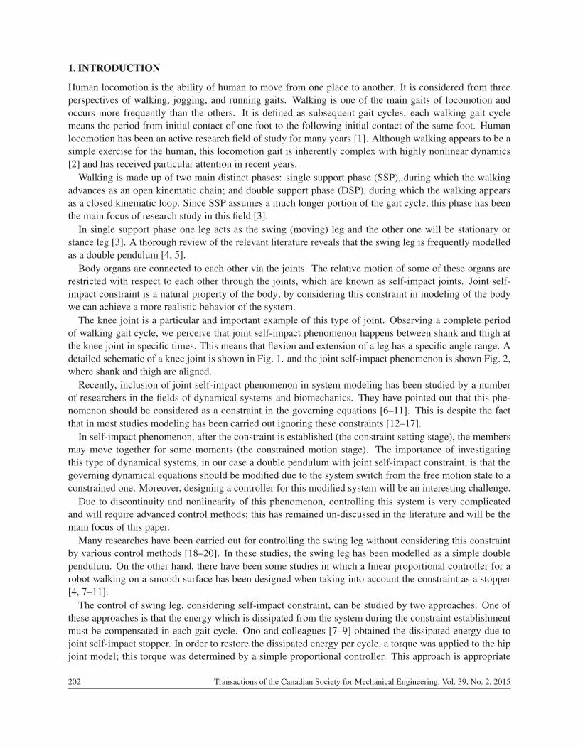
The knee joint is a particular and important example of this type of joint. Observing a complete periodof walking gait cycle, we perceive that joint self-impact phenomenon happens between shank and thigh atthe knee joint in specific times. This means that flexion and extension of a leg has a specific angle range. Adetailed schematic of a knee joint is shown in Fig. 1. and the joint self-impact phenomenon is shown Fig. 2,where shank and thigh are aligned.

Recently, inclusion of joint self-impact phenomenon in system modeling has been studied by a numberof researchers in the fields of dynamical systems and biomechanics. They have pointed out that this phe-nomenon should be considered as a constraint in the governing equations [6–11]. This is despite the factthat in most studies modeling has been carried out ignoring these constraints [12–17].

In self-impact phenomenon, after the constraint is established (the constraint setting stage), the membersmay move together for some moments (the constrained motion stage). The importance of investigatingthis type of dynamical systems, in our case a double pendulum with joint self-impact constraint, is that thegoverning dynamical equations should be modified due to the system switch from the free motion state to aconstrained one. Moreover, designing a controller for this modified system will be an interesting challenge.

Due to discontinuity and nonlinearity of this phenomenon, controlling this system is very complicatedand will require advanced control methods; this has remained un-discussed in the literature and will be themain focus of this paper.

Many researches have been carried out for controlling the swing leg without considering this constraintby various control methods [18–20]. In these studies, the swing leg has been modelled as a simple doublependulum. On the other hand, there have been some studies in which a linear proportional controller for arobot walking on a smooth surface has been designed when taking into account the constraint as a stopper[4, 7–11].

The control of swing leg, considering self-impact constraint, can be studied by two approaches. One ofthese approaches is that the energy which is dissipated from the system during the constraint establishmentmust be compensated in each gait cycle. Ono and colleagues [7–9] obtained the dissipated energy due tojoint self-impact stopper. In order to restore the dissipated energy per cycle, a torque was applied to the hipjoint model; this torque was determined by a simple proportional controller. This approach is appropriate

202 Transactions of the Canadian Society for Mechanical Engineering, Vol. 39, No. 2, 2015

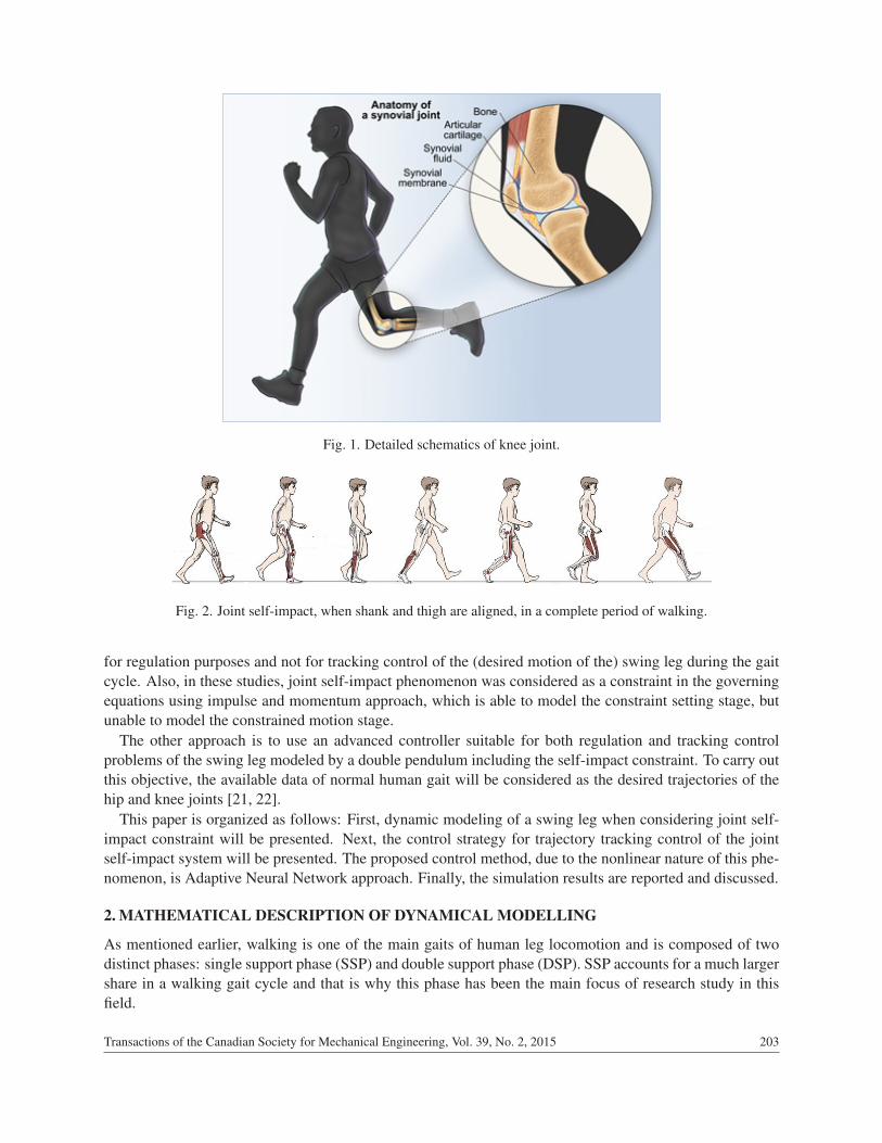
Fig. 1. Detailed schematics of knee joint.

Fig. 2. Joint self-impact, when shank and thigh are aligned, in a complete period of walking.

for regulation purposes and not for tracking control of the (desired motion of the) swing leg during the gaitcycle. Also, in these studies, joint self-impact phenomenon was considered as a constraint in the governingequations using impulse and momentum approach, which is able to model the constraint setting stage, butunable to model the constrained motion stage.

The other approach is to use an advanced controller suitable for both regulation and tracking controlproblems of the swing leg modeled by a double pendulum including the self-impact constraint. To carry outthis objective, the available data of normal human gait will be considered as the desired trajectories of thehip and knee joints [21, 22].

This paper is organized as follows: First, dynamic modeling of a swing leg when considering joint self-impact constraint will be presented. Next, the control strategy for trajectory tracking control of the jointself-impact system will be presented. The proposed control method, due to the nonlinear nature of this phe-nomenon, is Adaptive Neural Network approach. Finally, the simulation results are reported and discussed.

2. MATHEMATICAL DESCRIPTION OF DYNAMICAL MODELLING

As mentioned earlier, walking is one of the main gaits of human leg locomotion and is composed of twodistinct phases: single support phase (SSP) and double support phase (DSP). SSP accounts for a much largershare in a walking gait cycle and that is why this phase has been the main focus of research study in thisfield.


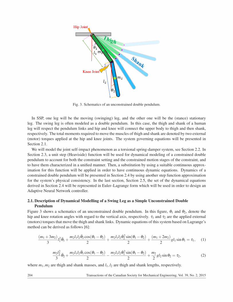
Fig. 3. Schematics of an unconstrained double pendulum.

In SSP, one leg will be the moving (swinging) leg, and the other one will be the (stance) stationaryleg. The swing leg is often modeled as a double pendulum. In this case, the thigh and shank of a humanleg will respect the pendulum links and hip and knee will connect the upper body to thigh and then shank,respectively. The total moments required to move the muscles of thigh and shank are denoted by two external(motor) torques applied at the hip and knee joints. The system governing equations will be presented inSection 2.1.

We will model the joint self-impact phenomenon as a torsional spring-damper system, see Section 2.2. InSection 2.3, a unit step (Heaviside) function will be used for dynamical modeling of a constrained doublependulum to account for both the constraint setting and the constrained motion stages of the constraint, andto have them characterized in a unified manner. Then, a substitution by using a suitable continuous approx-imation for this function will be applied in order to have continuous dynamic equations. Dynamics of aconstrained double pendulum will be presented in Section 2.4 by using another step function approximationfor the system’s physical consistency. In the last section, Section 2.5, the set of the dynamical equationsderived in Section 2.4 will be represented in Euler–Lagrange form which will be used in order to design anAdaptive Neural Network controller.

2.1. Description of Dynamical Modelling of a Swing Leg as a Simple Unconstrained DoublePendulum

Figure 3 shows a schematics of an unconstrained double pendulum. In this figure, θ1 and θ2, denote thehip and knee rotation angles with regard to the vertical axis, respectively. τ1 and τ2 are the applied external(motors) torques that move the thigh and shank links. Dynamic equations of this system based on Lagrange’smethod can be derived as follows [6]:

(m1 +3m2)

3l21 θ1 +

m2l1l2θ2 cos(θ1−θ2)

2+

m2l1l2θ 22 sin(θ1−θ2)

2+

(m1 +2m2)

2gl1 sinθ1 = τ1, (1)

m2l22

3θ2 +


2− m2l1l2θ 2

1 sin(θ1−θ2)

2+

m2

2gl2 sinθ2 = τ2, (2)

where m1,m2 are thigh and shank masses, and l1, l2 are thigh and shank lengths, respectively.


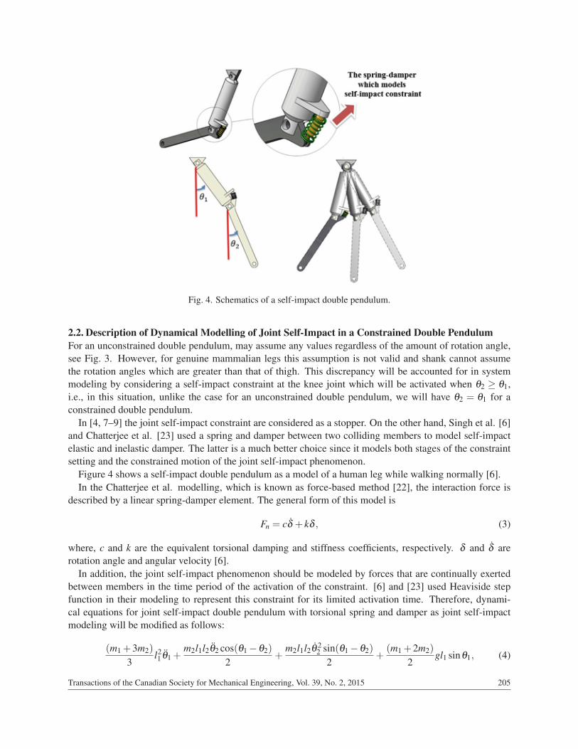
Fig. 4. Schematics of a self-impact double pendulum.

2.2. Description of Dynamical Modelling of Joint Self-Impact in a Constrained Double PendulumFor an unconstrained double pendulum, may assume any values regardless of the amount of rotation angle,see Fig. 3. However, for genuine mammalian legs this assumption is not valid and shank cannot assumethe rotation angles which are greater than that of thigh. This discrepancy will be accounted for in systemmodeling by considering a self-impact constraint at the knee joint which will be activated when θ2 ≥ θ1,i.e., in this situation, unlike the case for an unconstrained double pendulum, we will have θ2 = θ1 for aconstrained double pendulum.

In [4, 7–9] the joint self-impact constraint are considered as a stopper. On the other hand, Singh et al. [6]and Chatterjee et al. [23] used a spring and damper between two colliding members to model self-impactelastic and inelastic damper. The latter is a much better choice since it models both stages of the constraintsetting and the constrained motion of the joint self-impact phenomenon.

Figure 4 shows a self-impact double pendulum as a model of a human leg while walking normally [6].In the Chatterjee et al. modelling, which is known as force-based method [22], the interaction force is

described by a linear spring-damper element. The general form of this model is

Fn = cδ + kδ , (3)

where, c and k are the equivalent torsional damping and stiffness coefficients, respectively. δ and δ arerotation angle and angular velocity [6].

In addition, the joint self-impact phenomenon should be modeled by forces that are continually exertedbetween members in the time period of the activation of the constraint. [6] and [23] used Heaviside stepfunction in their modeling to represent this constraint for its limited activation time. Therefore, dynami-cal equations for joint self-impact double pendulum with torsional spring and damper as joint self-impactmodeling will be modified as follows:

(m1 +3m2)

3l21 θ1 +


2+


2+

(m1 +2m2)

2gl1 sinθ1, (4)


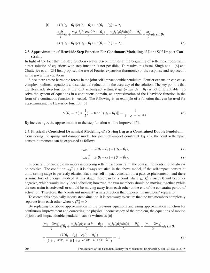
[t] +U(θ2−θ1)(k(θ1−θ2)+ c(θ1− θ2)) = τ1

m2l22

3θ2 +

m2l1l2θ1 cos9θ1−θ2)

2− m2l1l2θ 2

1 sin(θ1−θ2)

2+

m2

2gl2 sinθ2

+U(θ2−θ1)(k(θ2−θ1)+ c(θ2− θ1)) = τ2. (5)

2.3. Approximation of Heaviside Step Function For Continuous Modelling of Joint Self-Impact Con-straint

In light of the fact that the step function creates discontinuities at the beginning of self-impact constraint,direct solution of equations with step function is not possible. To resolve this issue, Singh et al. [6] andChatterjee et al. [23] first proposed the use of Fourier expansion (harmonic) of the response and replaced itin the governing equations.

Since there are no harmonic forces in the joint self-impact double pendulum, Fourier expansion can causecomplex nonlinear equations and substantial reduction in the accuracy of the solution. The key point is thatthe Heaviside step function at the joint self-impact setting stage (when θ2 = θ1) is not differentiable. Tosolve the system of equations in a continuous domain, an approximation of the Heaviside function in theform of a continuous function is needed. The following is an example of a function that can be used forapproximating the Heaviside function [6]

U(θ2−θ1)≈12(1+ tanh[r(θ2−θ1)]) =

11+ e−2r(θ2−θ1)

. (6)

By increasing r, the approximation to the step function will be improved [6].

2.4. Physically Consistent Dynamical Modelling of a Swing Leg as a Constrained Double PendulumConsidering the spring and damper model for joint self-impact constraint Eq. (3), the joint self-impactconstraint moment can be expressed as follows

fwdT 1ct = k(θ2−θ1)+(θ2− θ1), (7)

fwdT 2ct = k(θ1−θ2)+(θ1− θ2). (8)

In general, for two rigid members undergoing self-impact constraint, the contact moments should alwaysbe positive. The condition fwdT 1

ct > 0 is always satisfied in the above model, if the self-impact constraintat its setting stage is perfectly elastic. But since self-impact constraint is a passive phenomenon and thereis some loss of energy involved at this stage, there can be a point where fwdT 1

ct crosses 0 and becomesnegative, which would imply local adhesion; however, the two members should be moving together (whilethe constraint is activated) or should be moving away from each other at the end of the constraint period ofactivation. Therefore, the “constraint moment” is in a direction that opposes the members’ separation.

To correct this physically inconsistent situation, it is necessary to ensure that the two members completelyseparate from each other when fwdT 1

ct = 0.By replacing the above approximation in the previous equations and using approximation function for

continuous improvement and correcting the physical inconsistency of the problem, the equations of motionof joint self-impact double pendulum can be written as [6]

(m1 +3m2)

3l21 θ1 +


2+


2+

(m1 +2m2)

2gl1 sinθ1

+(k(θ1−θ2)+ c(θ1− θ2))

(1+ e−2r(θ2−θ1))(1+ e−2r(k(θ2−θ1)+c(θ2−θ1)))= τ1 (9)


m2l22

3θ2 +


2− m2l1l2θ 2

1 sin(θ1−θ2)

2+

m2

2gl2 sinθ2×

(k(θ2−θ1)+ c(θ2− θ1))

(1+ e−2r(θ2−θ1))(1+ e−2r(k(θ2−θ1)+c(θ2−θ1)))= τ2. (10)

2.5. Matrix Representation of Dynamical Equations of Joint Self-Impact Double PendulumThe dynamical equations of a swing leg, which is modelled as a constrained double pendulum, may berewritten in the following form

M(q)q+C(q, q)q+G(q)+ τ f (q, q) = τ, (11)

where q, q, q are 2× 1 vectors of joint angles, joint angular velocities, and joint angular accelerations, re-spectively; M(q) is 2×2 symmetric positive definite inertia matrix; C(q, q)q is 2×1 vector of Coriolis andcentrifugal torques satisfying M(q)−2C(q, q) is a skew-symmetric matrix; G(q) is 2×1 vector of gravita-tional torques; τ f (q, q) is 2×1 vector of approximated joint self-impact constraint moments and τ is 2×1vector of actuator joint torques.

M(q) =

(m1+3m2)3 l2

1m2l1l2 cos(θ1θ2)

2

m2l1l2 cos(θ1−θ2)2

m2l22

3

C(q, q) =

0 m2l1l2θ2 sin(θ1−θ2)2

−m2l1l2θ2 sin(θ1−θ2)2 0

G(q) =

[(m1+2m2)

2 gl1 sinθ1

m22 gl2 sinθ2

], τ f (q, q) =

(k(θ1−θ2)+c(θ1−θ2))

(1+e−2r(θ2−θ1))(1+e−2r(k(θ2−θ1)+c(θ2−θ1)))

(k(θ2−θ1)+c(θ2−θ1))

(1+e−2r(θ2−θ1))(1+e−2r(k(θ2−θ1)+c(θ2−θ1)))

, τ =

[τ1τ2

]

3. TRACKING CONTROL OF THE JOINT SELF-IMPACT SYSTEM

To the best of our knowledge, there has not been any publication on tracking control of any joint self-impactsystem. However, there are a few articles on regulation problem of the constrained double pendulum systemby some researchers [4, 7–11] and also by the authors of the current paper [24].

For the tracking problem, the gait cycles of normal walking taken from the available data as in [21,22] should be assigned as the desired trajectories of the thigh and knee joints of the constrained doublependulum.

Due to complex nonlinear terms in the dynamic equations of self-impact double pendulum, we pro-pose a nonlinear intelligent controller be designed by taking advantage of the Adaptive Neural Networkcontrol method, which requires neither the evaluation of the system inverse dynamical model nor the time-consuming training process.

There are a number of available control schemes in order to achieve accurate trajectory tracking andgood control performance. One of the most intuitive schemes which relies on the exact cancellation of thenonlinear dynamics of the manipulator system is computed torque control method.

The main disadvantage of this method is that the exact dynamic model is required. To overcome thedifficulties of this method, adaptive control strategies have been developed and have attracted the interest ofmany researches, see [25, 26] for an example. An advantage of the adaptive control methods is the priorknowledge of unknown parameters is not a requirement.


Fig. 5. Gaussian radial basis function.

To improve the performance of systems which have repetitive motions or operations, learning controlschemes have been developed [27]. A disadvantage of such a technique is that it is only applicable foroperations which have repetition so that learning can take place.

There have been some developments in the use of neural networks for control purposes [28–31]. Ingeneral, neural network control design has two steps. First the dynamic model of the system is approximatedusing neural network. Then, when this approximation, which is usually carried out off-line, is accurateenough, an appropriate control strategy can be constructed. It is important to note that this approach doesnot have any built-in capability to deal with the changes in the system; therefore, incorporation of adaptivecontrol is useful.

There have been some successful works by applying adaptive neural network (ANN) approach; they havebeen able to directly parameterize the control law by a suitable neural network [32, 33]. This has led toan overall closed-loop system with decent stability properties. Another advantage of this method is theevaluation of inverse dynamic model, as well as the time-consuming training process are no longer required[34, 35]. By assuming no prior knowledge about the system, the neural networks can be initialized in zerowith no problems. Also, ANN controller is robust and easy to use for real time implementation.

3.1. Adaptive Neural Network ControlIn the field of control engineering, neural network is often used to approximate a given nonlinear function upto a small error tolerance. In this paper, Gaussian radial basis function (RBF) neural network is considered.It is a particular network architecture which uses numbers of Gaussian function of the form [36]

ai(y)exp(−(y−µi)

T (y−µi)

σ2

), (12)

where µi ∈ Rn is the center vector and σ2 ∈ R is the variance. As shown in Fig. 5, each Gaussian RBFnetwork consists of three layers: the input layer, the hidden layer that contains the Gaussian function, andthe output layer. The output of the Network f (W,y) can be given by

f (W,y) =W T a(y) (13)


where a(y) = [a1(y) a2(y) . . . ,al(y)] is the vector of basis function. Note that only the connections from thehidden layer to the output are weighted.

Gaussian RBF network has been quite successful in representing the complex nonlinear functions. It hasbeen proven that any continuous function, not necessarily infinitely smooth, can be uniformly approximatedby a linear combination of Gaussians.

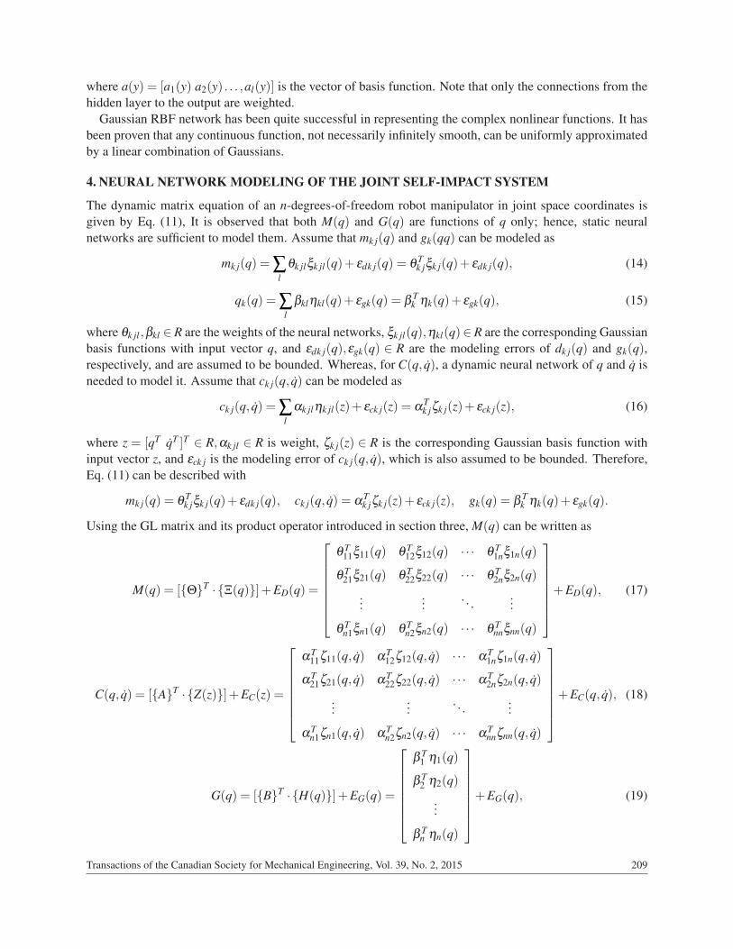
4. NEURAL NETWORK MODELING OF THE JOINT SELF-IMPACT SYSTEM

The dynamic matrix equation of an n-degrees-of-freedom robot manipulator in joint space coordinates isgiven by Eq. (11), It is observed that both M(q) and G(q) are functions of q only; hence, static neuralnetworks are sufficient to model them. Assume that mk j(q) and gk(qq) can be modeled as

mk j(q) = ∑l

θk jlξk jl(q)+ εdk j(q) = θTk jξk j(q)+ εdk j(q), (14)

qk(q) = ∑l

βklηkl(q)+ εgk(q) = βTk ηk(q)+ εgk(q), (15)

where θk jl,βkl ∈R are the weights of the neural networks, ξk jl(q),ηkl(q)∈R are the corresponding Gaussianbasis functions with input vector q, and εdk j(q),εgk(q) ∈ R are the modeling errors of dk j(q) and gk(q),respectively, and are assumed to be bounded. Whereas, for C(q, q), a dynamic neural network of q and q isneeded to model it. Assume that ck j(q, q) can be modeled as

ck j(q, q) = ∑l

αk jlηk jl(z)+ εck j(z) = αTk jζk j(z)+ εck j(z), (16)

where z = [qT qT ]T ∈ R,αk jl ∈ R is weight, ζk j(z) ∈ R is the corresponding Gaussian basis function withinput vector z, and εck j is the modeling error of ck j(q, q), which is also assumed to be bounded. Therefore,Eq. (11) can be described with

mk j(q) = θTk jξk j(q)+ εdk j(q), ck j(q, q) = α

Tk jζk j(z)+ εck j(z), gk(q) = β

Tk ηk(q)+ εgk(q).

Using the GL matrix and its product operator introduced in section three, M(q) can be written as

M(q) = [{Θ}T · {Ξ(q)}]+ED(q) =

θ T

11ξ11(q) θ T12ξ12(q) · · · θ T

1nξ1n(q)

θ T21ξ21(q) θ T

22ξ22(q) · · · θ T2nξ2n(q)

......

. . ....

θ Tn1ξn1(q) θ T

n2ξn2(q) · · · θ Tnnξnn(q)

+ED(q), (17)

C(q, q) = [{A}T · {Z(z)}]+EC(z) =

αT

11ζ11(q, q) αT12ζ12(q, q) · · · αT

1nζ1n(q, q)

αT21ζ21(q, q) αT

22ζ22(q, q) · · · αT2nζ2n(q, q)

......

. . ....

αTn1ζn1(q, q) αT

n2ζn2(q, q) · · · αTnnζnn(q, q)

+EC(q, q), (18)

G(q) = [{B}T · {H(q)}]+EG(q) =

β T

1 η1(q)

β T2 η2(q)

...

β Tn ηn(q)

+EG(q), (19)


where {Θ},{Ξ(q)},{A},{Z(z)},{B} and {H(q)} are the GL matrices with their elements beingθk j,ξk j(q),αk j,ζk j(z),βk and ηk(q) respectively, as defined in Appendix A, and ED(q)∈ Rn×n,EC(z)∈ Rn×n

and EG(q) ∈ Rn are the matrices with their elements being the modeling errors εdk j(q),εck j(z) and εgk(q),respectively.

5. CONTROL SYSTEM DESIGN

Let qd(t) be the desired trajectory in the joint space and qd(t) and qd(t) be the desired velocity and acceler-ation. Define

e(t) = qd(t)−q(t), (20)

qr(t) = qd(t)+qυ +Λe(t), (21)

r(t) = qr(t)− q(t) = e(t)+Λe(t), (22)

where Λ is a positive definite matrix. According to the lemma, represented in [36], the stability of e and ecan be concluded by studying r.

Denote the estimate of by , and define Hence, and represent the estimates of the true parameter matricesand respectively. The control law can be proposed to have the following form [36]:

τ = [{Θ}T · {Ξ(q)}]qr +[{A} · {Z(z)}]qr +[{B}T · {H(q)}]+Kr+ ks sgn(r), (23)

where K ∈ Rn×n and ks > ||E||, with E = ED(q)qr +EC(z)qr +EG(q)+ τ f (q, q). The first three terms ofthe control law are the model-based control, whereas the Kr term gives the proportional derivative (PD)type of control. Note that the PD control is effectively introduced to the control law through the definitiongiven in Eq. (22). The last term in the control law is added to suppress the modeling errors of the neuralnetworks. The parameters in the control law are updated according to the proof of stability and convergencyrequirements presented in Appendix B:

˙θ = Γk · {ξk(q)}qrrk, (24)˙α = Qk · {ζk(z)}qrrk, (25)

˙β = Nkηk(q)rk, (26)

where Γk,Qk and Nk are positive definite and symmetric; and θ and α are the column vectors with theirelements being θk j and ˆal phak j , respectively.

6. SIMULATION AND DISCUSSION

Table 1 shows the parameters that are used to simulate the locomotion of a swing leg as a self-impact doublependulum. The anthropometric dimensions and masses match the parameters presented in [22].

6.1. The Gait Cycles of Normal Walking Taken as the Desired Joint Angles of the Hip and KneeJoints

For the tracking problem the desired trajectories of the thigh and knee joints of the self-impact doublependulum, representing the swing leg during normal walking, should be taken from the available normalgait cycle data [21, 22].

These curves are presented in Fig. 6 and the period in which joint self-impact phenomenon occurs ishighlighted.

According to this figure, joint self-impact phenomenon for joint self-impact double pendulum systemhappens when the knee rotation angle is greater than that of the hip.

Taking the time derivative of the above curves, the desired angular velocities of the hip and knee jointswill be obtained (see Fig. 7).


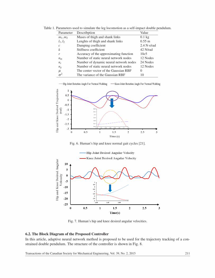
Table 1. Parameters used to simulate the leg locomotion as a self-impact double pendulum.Parameter Describption Valuem1,m2 Mases of thigh and shank links 0.1 kgl1, l2 Lenghts of thigh and shank links 0.55 mc Damping coefficient 2.4 N·s/radk Stiffness coefficient 42 N/radr Accuracy of the approximating function 10e5nm Number of static neural network nodes 12 Nodesnc Number of dynamic neural network nodes 24 Nodesng Number of static neural network nodes 12 Nodesµ The center vector of the Gaussian RBF 0σ2 The variance of the Gaussian RBF 10

Fig. 6. Human’s hip and knee normal gait cycles [21].

Fig. 7. Human’s hip and knee desired angular velocities.

6.2. The Block Diagram of the Proposed ControllerIn this article, adaptive neural network method is proposed to be used for the trajectory tracking of a con-strained double pendulum. The structure of the controller is shown in Fig. 8.


Fig. 8. The structure of the adaptive neural network controller.

Fig. 9. Hip joint desired and tracked trajectories.

Fig. 10. Time history of hip joint angle error.

6.3. Self-Impact Double Pendulum Simulation ResultsThe purpose of the present study is to simulate the tracking control of the self-impact double pendulum.Figure 9 shows the hip joint desired and tracked trajectories; it can be realized that the swing leg has followedthe desired values for its hip joint very closely which is well followed by the swing leg. Time history of hip


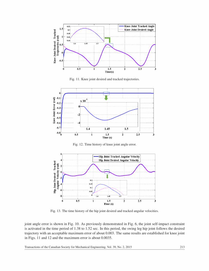
Fig. 11. Knee joint desired and tracked trajectories.

Fig. 12. Time history of knee joint angle error.

Fig. 13. The time history of the hip joint desired and tracked angular velocities.

joint angle error is shown in Fig. 10. As previously demonstrated in Fig. 6, the joint self-impact constraintis activated in the time period of 1.38 to 1.52 sec. In this period, the swing leg hip joint follows the desiredtrajectory with an acceptable maximum error of about 0.003. The same results are established for knee jointin Figs. 11 and 12 and the maximum error is about 0.0035.


Fig. 14. Time history of the error of the hip joint angular velocity.

Fig. 15. The time history of the knee joint desired and tracked angular velocities.

Fig. 16. Time history of the error of the knee joint angular velocity.

As it can be seen in Figs 9–12, the performance of controller is acceptable. Also noted in the figures,when the constraint is activated, the hip and knee joint angular velocity and the applied torque of the motorsuddenly change in both joints. Despite these sudden changes, the controller follows the trajectories of thighand knee joints accurately.

Figure 13 shows the velocity of swing leg together with the desired angular velocity of the hip joint. Asseen in the figure, in the time period of 1.38 to 1.52 sec, the swing leg encounters a sudden change in itsspeed, which is caused by an increase in the angular momentum of the link due to the establishment of theconstraint. The controller has matched the hip joint speed to its desired value with the maximum error ofabout 0.075 (Fig. 14). The same results are illustrated for knee joint in Figs. 15 and 16. For knee jointvelocity, the maximum error is about 0.12.


Fig. 17. Hip joint torque.

Fig. 18. Knee joint torque.

Figures 17 and 18 represent the amount of torque applied by the motors embedded in the hip and kneejoints, respectively. When joint self-impact constraint is activated, the moment caused by the establishmentof the constraint is in the same direction of the motor torque of the hip joint, which causes the motor toprovide less torque to track the path. These figures show the sudden drop in the amount of torque.

7. CONCLUSIONS

The objective of this paper was to present a model-based control method for trajectory tracking of a con-strained double pendulum which modeled the swing leg in normal human walking, by considering the jointself-impact constraint. To achieve this objective, first, the dynamical equations of motion of an uncon-strained double pendulum were taken and then developed and modified to account for the joint self-impactconstraint at the knee joint. Two approximations of the Heaviside step function were applied to the equa-tions of motion in order to account for continuity and physical consistency of the derived set of equationsof motion. To control this complicated system, the available normal gait cycle data were taken to generatethe desired trajectories of the thigh and knee joints of the self-impact double pendulum. Due to complexnonlinear terms in the dynamical governing equations of self-impact double pendulum, we propose a nonlin-ear intelligent controller be designed by taking advantage of the Adaptive Neural Network control method,which requires neither the evaluation of inverse dynamical model nor the time-consuming training process.

According to the simulation results, the normal gait cycle data of the rotation angles of the hip and kneejoints were well followed by the simulated constrained double pendulum. The joint self-impact constraintwas activated in the time period of 1.38 to 1.52 sec. In this period, even in the presence of the suddenchanges in the hip and knee kinematic variables at the constraint activation stage, the swing leg hip andknee joints tracked the desired values of the rotation angles with an acceptable maximum error of about


0.007% and 0.013%, respectively. Comparable results were obtained for the joints angular velocity with anacceptable maximum error of about 0.15% for the hip joint and 0.35% for the knee joint.

REFERENCES

1. Zhang, D. and Zhu, K., “Model and control of the locomotion of a biomimic musculoskeletal biped”, ArtificialLife and Robotics, Vol. 10, No. 2, pp. 91–95, 2006.

2. Rose, J. and Gibson Gamble, J. (Eds.), Human Walking, Lippincott Williams & Wilkins, Philadelphia, 2006.3. Ayyappa, E., “Normal human locomotion, Part 1: Basic concepts and terminology”, JPO: Journal of Prosthetics

and Orthotics, Vol. 9, No. 1, pp. 10–17, 1997.4. Huang, Q and Ono, K., “Energy-efficient walking for biped robot using self-excited mechanism and optimal

trajectory planning”, in Humanoid Robots, New Developments, pp. 582, 2007.5. Goswami, A., Bernard, E. and Ahmed, K., “Limit cycles in a passive compass gait biped and passivity-mimicking

control laws”, Autonomous Robots, Vol. 4, No. 3, pp. 273–286, 1997.6. Singh, S., Mukherjee, S. and Sanghi, S., “Study of a self-impacting double pendulum”, Journal of Sound and

Vibration, Vol. 318, No. 4, pp. 1180–1196, 2008.7. Ono, K. et al., “Self-excitation control for biped walking mechanism”, Intelligent Robots and Systems (IROS

2000), Vol. 2. IEEE, 2000.8. Ono, K., Takahashi, R. and Shimada, T., “Self-excited walking of a biped mechanism”, The International Journal

of Robotics Research, Vol. 20, No. 12, pp. 953–966, 2001.9. Ono, K., Furuichi, T. and Takahashi, R., “Self-excited walking of a biped mechanism with feet”, The Interna-

tional Journal of Robotics Research, Vol. 23, No. 1, pp. 55–68, 2004.10. Sangwan, V., Taneja, A. and Mukherjee, S., “Design of a robust self-excited biped walking mechanism”, Mech-

anism and Machine Theory, Vol. 39, No. 12, pp. 1385–1397, 2004.11. Mukherjee, S., Sangwan, V., Taneja, A. and Seth, B., “Stability of an underactuated bipedal gait”, Biosystems,

Vol. 90, No. 2, pp. 582–589, 2007.12. Couceiro, M.S., Ferreira, N.M.F. and Machado, J.A., “Hybrid adaptive control of a dragonfly model”, Commu-

nications in Nonlinear Science and Numerical Simulation, Vol. 17, No. 2, pp. 893–903, 2012.13. Cross, R., “A double pendulum model of tennis strokes”, American Journal of Physics, Vol. 79, p. 470, 2011.14. Miller, R.H., “Optimal control of human running”, in An Optimal Control Model for Human Postural Regulation,

2011.15. Couceiro, M.S., Fonseica Ferreira, N.M. and Tenreiro Machado, J.A., “Modeling and control of a dragonfly-like

robot”, in Computational Intelligence for Engineering Systems, pp. 104–118, Springer, the Netherlands, 2011.16. Couceiro, M.S., Fonseca Ferreira, N.M. and Tenreiro Machado, J.A., “Fractional-order control of a robotic

bird”, in Proceedings of IDETC/CIE 2009 ASME 2009 International Design Engineering Technical Conferences& Computers and Information in Engineering Conference, August 2009.

17. Couceiro, M.S. et al., “Simulation of a robotic bird”, in Proceedings of the 3rd IFAC Workshop on FractionalDifferentiation and Its Applications, 2008.

18. Blum, Y. et al., “Swing leg control in human running”, Bioinspiration & Biomimetics, Vol. 5, No. 2, 026006,2010.

19. Blum, Y., Juergen R. and Andre, S., “Advanced swing leg control for stable locomotion”, in Autonome MobileSysteme 2007, pp. 301–307, Springer, Berlin/Heidelberg, 2007.

20. Blum, Y., Birn-Jeffery, A., Daley, M.A. and Seyfarth, A., “Does a crouched leg posture enhance running stabilityand robustness?”, Journal of Theoretical Biology, Vol. 281, No. 1, pp. 97–106, 2011.

21. Ounpuu, S., “The biomechanics of walking and running”, Clin. Sports Med., Vol. 13, No. 4, pp. 843–863, 1994.22. McCaw, S.T., “Introduction to Biomechanics”, Foundations of Exercise Science, p. 155, 2001.23. Chatterjee, A.K. and Mallik, A.G., “On impact dampers for non-linear vibrating systems”, Journal of Sound and

Vibration, Vol. 187, No. 3, pp. 403–420, 1995.24. Bazargan-Lari, Y., Gholipour, A., Eghtesad, M., Nouri, M. and Sayadkooh, A., “Dynamics and control of loco-

motion of one leg walking as self-impact double pendulum”, in Proceedings 2nd International Conference onControl, Instrumentation and Automation (ICCIA), pp. 201–206, IEEE, 2011.

25. Craig, J.J., Hsu, P. and Sastry, S.S., “Adaptive control of mechanical manipulators”, Int. J. Robotics Res., Vol. 6,No. 2, pp. 16–28, 1987.


26. Slotine, J.J.E. and Li, W., “On the adaptive control of robot manipulators”, Int. J. Robotics Res., Vol. 6, No. 3,pp. 49–59, 1987.

27. Arimoto, S., “Learning control theory for robot motion”, Int. J. Adapt. Control Signal Process, Vol. 4, No. 6,pp. 543–564, 1990.

28. Miller, W.T., Glanz, F.H. and Kraft, I.G., “Application of a general learning algorithm to control of a roboticmanipulator”, Int. J. Robotics Res., Vol. 6, No. 2, pp. 84–98, 1987.

29. Miyamoto, H., Kawato, M., Setoyama, T. and Suzuki, R., “Feedback error learning neural network for trajectorycontrol of a robotic manipulator”, Neural Networks, Vol. 1, No. 3, pp. 251–265, 1988.

30. Ozaki, T., Suzuki, T., Furuhashi, T., Okuma, S. and Uchikawa, Y., “Trajectory control of robotic manipulatorsusing neural networks”, IEEE Trans. Ind. Electron., Vol. 38, pp. 195–202, 1991.

31. Saad, M., Dessaint, L.A., Bigras, P. and Al-haddad K., “Adaptive versus neural network adaptive control: appli-cation to robotics”, Int. J. Adapt. Control Signal Process, Vol. 8, No. 3, pp. 223–236, 1994.

32. Sanner, R.M. and Slotine, J.J.E., “Gaussian networks for direct adaptive control”, IEEE Trans. Neural Networks,Vol. 3, pp. 837–863, 1992.

33. Tzirkel-Hancock, E. and Fallside, F., “A direct control method for a class of nonlinear systems using neuralnetwork”, Rep. CUED/F-INFENG/TR65, Cambridge Univ., Cambridge, U.K., 1991.

34. Lewis, F.L., Liu, K. and Yesildirek, A., “Neural net robot controller with guaranteed tracking performance”,IEEE Trans. Neural Networks, Vol. 6, pp. 703–715, 1995.

35. Ge, S.S. and Hang, C.C., “Direct adaptive neural network control of robots”, Int. J. Syst. Sci., Vol. 27, No. 6,pp. 533–542, 1996.

36. Wei, L.X., Yang, L., and Wang, H.R., “Adaptive neural network position/force control of robot manipulatorswith model uncertainties”, in Proceedings Neural Networks and Brain, ICNN&B’05, Vol. 3, pp. 1825–1830,2005.

APPENDIX A: GL MATRIX AND OPERATOR

In this section, the definition of GL matrix, denoted by {·} and its product operator “·” are briefly discussed.To avoid any possible confusion, [·] isued to denote the ordinary vector and matrix [36].

Let I0 be the set of integers and θk j,ξk j ∈ Rnk j , where nk j ∈ I0, j = 1,2, . . . ,n, k = 1,2, . . . ,n. The GL rowvector {θk} and its transpose {θk}T are defined in the following way:

{θk}= {θk1 θk2 · · · θkn}, {θk}T = {θ Tk1 θ

Tk2 θ

Tkn}. (27)

The GL matrix {Θk} and its transpose {ΘTk } are defined accordingly as

{Θk}=

θ11quad θ12 · · · θ1n

θ21 θ22 · · · θ2n

......

. . ....

θn1 θn2 · · · θnn

=

{θ1}

{θ2}...

{θn}

, {ΘT

k }=

θ T11 θ T

12 · · · θ T1n

θ T21 θ T

22 · · · θ T2n

......

. . . · · ·

θ Tn1 θ T

n2 · · · θ Tnn

=

{θ T1 }

{θ T2 }...

{θ Tn }

.

(28)For a given GL matrix {Ξ}

{Ξ}=

ξ11 ξ12 · · · ξ1n

ξ21 ξ22 · · · ξ2n

· · · · · · . . ....

ξn1 ξn2 · · · ξnn

=

{ξ1}

{ξ2}...

{ξn}

. (29)


The GL product of {Θk}T and {Ξ} is n×n matrix defined as

[{Θk}T · {Ξ}] =

θ T

11ξ11 θ T12ξ12 · · · θ T

1nξ1n

θ T21ξ21 θ T

22ξ22 · · · θ T2nξ2n

......

. . ....

θ Tn1ξn1 θ T

n2ξn2 · · · θ Tnnξnn

. (30)

The GL product of a square matrix and a GL row vector is defined as follows. Let

Γk = ΓTk = [γk1 γk2 · · · γkn], γk j ∈ Rm×nk j , m =

n

∑j=1

nk j

then we haveΓk · {ξ1}= {Γk} · {ξ1}= [γk1ξk1 γk2ξk2 · · · γknξkn] ∈ Rm×n. (31)

Note that the GL product should be computed first in a mixed matrix product. For instance, in {A} · {B}C,the matrix {A} · {B} should be computed first, and then followed by the multiplication of {A} · {B} withmatrix C.

APPENDIX B: PROOF OF STABILITY

Applying the control law, Eq. (23), to the system dynamics, Eq. (11), and using the definition of the filteredtracking error, Eq. (22), yields the following tracking error dynamics

M(q)r+C(q, q)r+Kr+ kssgn(r) = [{Θ}T · {Ξ(q)}]q¨

r +[{A}T · {Z(z)}]qr +[{B}T · {H(q)}]+E. (32)

Consider the nonnegative scalar function V as

V =12

rT M(q)r+12

n

∑k=1

θTk Γ−1k θk +

12

n

∑k=1

αTk Q−1

k αk +12

n

∑k=1

βTk N−1

k βk, (33)

where Γk,Qk and Nk are dimensional compatible symmetric positive-definite matrices. Computing thederivative of Eq. (33) along Eq. (32) and simplifying yields

V = rT (M(q)r+C(q, q)r)+n

∑k=1

θTk Γ−1k

˙θk +

n

∑k=1

αTk Q−1

k˙αk +

n

∑k=1

βTk N−1

k˙βk, (34)

where the property of skew-symmetric has been used. Substituting the error equation Eq. (32) and notingthat

[{Θ} · {Ξ(q)}]qr =n

∑k=1{θk}T · {ξk(q)}qrrk, (35)

[{A} · {Z(z)}]qr =n

∑k=1{αk}T · {ζk(z)}qrrk, (36)

[{B} · {H(q)}] =n

∑k=1

βTk ηk(q)rk. (37)


Eq. (34) becomes

V = −rT Kr− ksrT sgn(r)+n

∑k=1{θk}T · {ξk(q)}qrrk +

n

∑k=1{αk}T · {ζk(z)}qrrk

n

∑k=1

βTk ηk(q)rk + rT E +

n

∑k=1

θTk Γ−1k

˙θk +

n

∑k=1

αTk Q−1

k˙αk +

n

∑k=1

βTk N−1

k˙βk. (38)

In order to make the time derivative of the Lyapunov function be negative-definite, the weight parameterupdate laws should be chosen as presented in Eqs. (24–26). Substituting the weight parameter update lawsinto Eq. (38), with ks > ‖E‖ yields

V ≤ rT Kr ≤ 0 (39)


double-pendulum considering self-impact joint constraint · adaptive neural network control of a...

Documents