A&A 645, L12 (2021)https://doi.org/10.1051/0004-6361/202039966c© ESO 2021

Astronomy&Astrophysics

LETTER TO THE EDITOR

Downflowing umbral flashes as evidence of standing waves insunspot umbrae

T. Felipe1,2, V. M. J. Henriques3,4, J. de la Cruz Rodríguez5, and H. Socas-Navarro1,2

1 Instituto de Astrofísica de Canarias, 38205 C/ Vía Láctea, s/n, La Laguna, Tenerife, Spaine-mail: tobias@iac.es

2 Departamento de Astrofísica, Universidad de La Laguna, 38205 La Laguna, Tenerife, Spain3 Institute of Theoretical Astrophysics, University of Oslo, PO Box 1029 Blindern, 0315 Oslo, Norway4 Rosseland Centre for Solar Physics, University of Oslo, PO Box 1029 Blindern, 0315 Oslo, Norway5 Institute for Solar Physics, Dept. of Astronomy, Stockholm University, AlbaNova University Centre, 10691 Stockholm, Sweden

Received 23 November 2020 / Accepted 6 January 2021

ABSTRACT

Context. Umbral flashes are sudden brightenings commonly visible in the core of some chromospheric lines. Theoretical and numer-ical modeling suggests that they are produced by the propagation of shock waves. According to these models and early observations,umbral flashes are associated with upflows. However, recent studies have reported umbral flashes in downflowing atmospheres.Aims. We aim to understand the origin of downflowing umbral flashes. We explore how the existence of standing waves in the umbralchromosphere impacts the generation of flashed profiles.Methods. We performed numerical simulations of wave propagation in a sunspot umbra with the code MANCHA. The Stokes profilesof the Ca ii 8542 Å line were synthesized with the NICOLE code.Results. For freely propagating waves, the chromospheric temperature enhancements of the oscillations are in phase with velocity up-flows. In this case, the intensity core of the Ca ii 8542 Å atmosphere is heated during the upflowing stage of the oscillation. However,a different scenario with a resonant cavity produced by the sharp temperature gradient of the transition region leads to chromosphericstanding oscillations. In this situation, temperature fluctuations are shifted backward and temperature enhancements partially coincidewith the downflowing stage of the oscillation. In umbral flash events produced by standing oscillations, the reversal of the emissionfeature is produced when the oscillation is downflowing. The chromospheric temperature keeps increasing while the atmosphere ischanging from a downflow to an upflow. During the appearance of flashed Ca ii 8542 Å cores, the atmosphere is upflowing most ofthe time, and only 38% of the flashed profiles are associated with downflows.Conclusions. We find a scenario that remarkably explains the recent empirical findings of downflowing umbral flashes as a naturalconsequence of the presence of standing oscillations above sunspot umbrae.

Key words. methods: numerical – Sun: chromosphere – Sun: oscillations – sunspots – techniques: polarimetric

1. Introduction

Oscillations are a ubiquitous phenomenon in the Sun. Their sig-natures have been detected almost everywhere, from the solarinterior to the outer atmosphere. One of the most spectacularmanifestations of solar oscillations are umbral flashes (UFs).They were discovered by Beckers & Tallant (1969; see alsoWittmann 1969), who observed them in sunspot umbrae asperiodic brightness enhancements in the core of some chromo-spheric spectral lines. Following their first detection, UFs wereassociated with magneto-acoustic wave propagation in umbralatmospheres (Beckers & Tallant 1969), and soon after Havnes(1970) suggested that UFs in Ca ii lines were formed due tothe temperature enhancement during the compressional stage ofthese waves.

The analysis of spectropolarimetric data has become a com-mon approach in the study of UFs over the last two decades,since the studies undertaken by Socas-Navarro et al. (2000a,b).They found anomalous polarization in the Stokes profiles andinterpreted it as indirect evidence of very fine structure in UFs,

unresolved in arc-second resolution observations. Their modelhad one hot upflowing component embedded in a cool down-flowing medium. Further independent, but still indirect, evidenceof such fine structure was obtained by Centeno et al. (2005).Subsequent studies, benefiting from observations acquired withhigher spatio-temporal resolution, were able to resolve thosecomponents in imaging observations (Socas-Navarro et al. 2009;Henriques & Kiselman 2013; Bharti et al. 2013; Yurchyshyn et al.2014; Henriques et al. 2015) and in full spectropolarimetric obse-rvations (Rouppe van der Voort & de la Cruz Rodríguez 2013;de la Cruz Rodríguez et al. 2013; Nelson et al. 2017). Non-local thermodynamical equilibrium (NLTE) inversions ofCa ii 8542 Å sunspot observations using the NICOLE code(Socas-Navarro et al. 2015) have found that UF atmospheres areassociated with temperature increments of around 1000 K andstrong upflows (de la Cruz Rodríguez et al. 2013). These observa-tional measurements exhibit a good agreement with the theoreticalpicture of UFs as a manifestation of upward propagating slowmagneto-acoustic waves. The amplitude of these waves increaseswith height as a result of the density stratification, leading to

Article published by EDP Sciences L12, page 1 of 7

A&A 645, L12 (2021)

the development of chromospheric shocks (Centeno et al. 2006;Felipe et al. 2010a) and UFs (Bard & Carlsson 2010; Felipe et al.2014). The properties of those UF shocks have recently beenevaluated by interpreting spectropolarimetric observations withthe support of the Rankine-Hugoniot relations (Anan et al. 2019;Houston et al. 2020).

The first NLTE inversions of UFs (Socas-Navarro et al.2001) were computationally very expensive (typically severalhours per individual spectrum), and therefore only a few pro-files from the same location and different times were inverted.Later improvements in code optimization, parallelization, andcomputer hardware allowed de la Cruz Rodríguez et al. (2013)to analyze a few 2D maps with spatial resolution. As thistrend continued, it is now possible to make UF studies withhigher spatial and temporal resolution and much better statistics(e.g., Henriques et al. 2017; Joshi & de la Cruz Rodríguez 2018;Houston et al. 2018, 2020). These recent results have revealedthe existence of UFs whose Stokes profiles are better reproducedwith atmospheres dominated by downflows (Henriques et al.2017; Bose et al. 2019; Houston et al. 2020).

Accommodating the downflowing UFs in the widelyaccepted scenario of upward propagating shock waves is atheoretical challenge. Studies employing sophisticated synthe-sis tools and numerical simulations of the umbral atmospherehave validated the upflowing UF model (Bard & Carlsson 2010;Felipe et al. 2014, 2018a; Felipe & Esteban Pozuelo 2019). Inthose simulations, magneto-acoustic waves can propagate fromthe photosphere to the chromosphere. According to the phaserelations of these propagating waves, velocity and tempera-ture oscillations exhibit opposite phases (considering that pos-itive velocities correspond to downflows), and the temperatureincrease responsible for the flash matches an upflow. How-ever, recent studies have shown evidence of a resonant cav-ity above sunspot umbrae (see Jess et al. 2020a,b; Felipe 2021;Felipe et al. 2020). This cavity is produced by wave reflectionsat the strong temperature gradient in the transition region (e.g.,Zhugzhda & Locans 1981; Zhugzhda 2008). Waves trapped ina resonant cavity produce standing oscillations whose temper-ature fluctuations are delayed by a quarter period with respectto the velocity signal, instead of the half-period delay fromfreely propagating waves (Deubner 1974; Felipe et al. 2020).In this study, we use numerical simulations and full-StokesNLTE radiative transfer calculations to explore the generationof intensity emission cores in the Ca ii 8542 Å line during thedownflowing stage of standing umbral oscillations, as well ashow they can support the existence of the recently reporteddownflowing UFs.

2. Numerical methods

Nonlinear wave propagation between the solar interiorand the corona was simulated using the code MANCHA(Khomenko & Collados 2006; Felipe et al. 2010b) in a 2Ddomain. The details of the simulations can be found inAppendix A. We computed synthetic full-Stokes spectra in theCa ii 8542 Å line taking snapshots from our numerical simu-lation and then computing the spectra with the NICOLE code(Socas-Navarro et al. 2015, see details in Appendix B). The codeassumes statistical equilibrium. Wedemeyer-Böhm & Carlsson(2011) showed that nonequilibrium effects in Ca ii are smallat the formation height of the infrared triplet lines, and, there-fore, statistical equilibrium should suffice to model Ca ii atoms.We calculated the transition probabilities between levels forCa ii in a sunspot model. They indicate characteristic transition

times much shorter than one second (Appendix B), meaning thatdepartures from statistical equilibrium are insignificant for thedynamics studied here.

3. Results

We analyzed how UFs are generated in the case of propagatingand standing oscillations. In Appendix C, we discuss the differ-ences in the phase relations between temperature and velocityfluctuations from propagating and standing waves as determinedfrom the analysis of numerical simulations. In the following,for the examination of the propagating-wave case, we focus onthe first wavefront of the simulation reaching the chromosphere,before any previous wavefronts are reflected and a standing waveis settled. We chose to follow this approach (instead of usingan independent simulation without transition region) in orderto employ exactly the same atmospheric stratification for bothcases. This way, we can ensure that the differences in the prop-erties of the UFs are produced by the nature of the oscillationsand not by the changes in the background atmospheres.

3.1. Umbral flashes from propagating waves

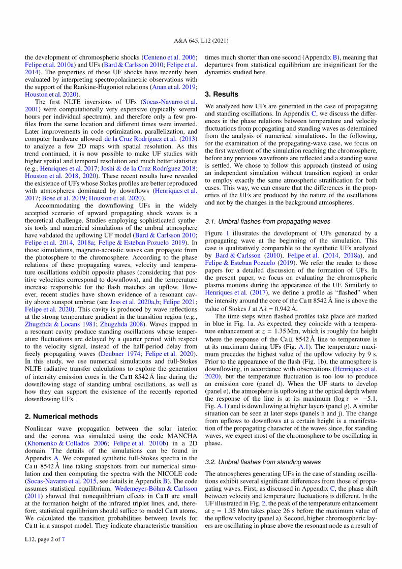
Figure 1 illustrates the development of UFs generated by apropagating wave at the beginning of the simulation. Thiscase is qualitatively comparable to the synthetic UFs analyzedby Bard & Carlsson (2010), Felipe et al. (2014, 2018a), andFelipe & Esteban Pozuelo (2019). We refer the reader to thosepapers for a detailed discussion of the formation of UFs. Inthe present paper, we focus on evaluating the chromosphericplasma motions during the appearance of the UF. Similarly toHenriques et al. (2017), we define a profile as “flashed” whenthe intensity around the core of the Ca ii 8542 Å line is above thevalue of Stokes I at ∆λ = 0.942 Å.

The time steps when flashed profiles take place are markedin blue in Fig. 1a. As expected, they coincide with a tempera-ture enhancement at z = 1.35 Mm, which is roughly the heightwhere the response of the Ca ii 8542 Å line to temperature isat its maximum during UFs (Fig. A.1). The temperature maxi-mum precedes the highest value of the upflow velocity by 9 s.Prior to the appearance of the flash (Fig. 1b), the atmosphere isdownflowing, in accordance with observations (Henriques et al.2020), but the temperature fluctuation is too low to producean emission core (panel d). When the UF starts to develop(panel e), the atmosphere is upflowing at the optical depth wherethe response of the line is at its maximum (log τ ≈ −5.1,Fig. A.1) and is downflowing at higher layers (panel g). A similarsituation can be seen at later steps (panels h and j). The changefrom upflows to downflows at a certain height is a manifesta-tion of the propagating character of the waves since, for standingwaves, we expect most of the chromosphere to be oscillating inphase.

3.2. Umbral flashes from standing waves

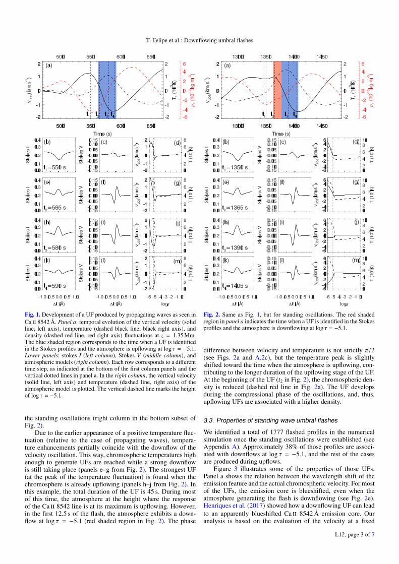
The atmospheres generating UFs in the case of standing oscilla-tions exhibit several significant differences from those of propa-gating waves. First, as discussed in Appendix C, the phase shiftbetween velocity and temperature fluctuations is different. In theUF illustrated in Fig. 2, the peak of the temperature enhancementat z = 1.35 Mm takes place 26 s before the maximum value ofthe upflow velocity (panel a). Second, higher chromospheric lay-ers are oscillating in phase above the resonant node as a result of

L12, page 2 of 7

T. Felipe et al.: Downflowing umbral flashes

Fig. 1. Development of a UF produced by propagating waves as seen inCa ii 8542 Å. Panel a: temporal evolution of the vertical velocity (solidline, left axis), temperature (dashed black line, black right axis), anddensity (dashed red line, red right axis) fluctuations at z = 1.35 Mm.The blue shaded region corresponds to the time when a UF is identifiedin the Stokes profiles and the atmosphere is upflowing at log τ = −5.1.Lower panels: stokes I (left column), Stokes V (middle column), andatmospheric models (right column). Each row corresponds to a differenttime step, as indicated at the bottom of the first column panels and thevertical dotted lines in panel a. In the right column, the vertical velocity(solid line, left axis) and temperature (dashed line, right axis) of theatmospheric model is plotted. The vertical dashed line marks the heightof log τ = −5.1.

the standing oscillations (right column in the bottom subset ofFig. 2).

Due to the earlier appearance of a positive temperature fluc-tuation (relative to the case of propagating waves), tempera-ture enhancements partially coincide with the downflow of thevelocity oscillation. This way, chromospheric temperatures highenough to generate UFs are reached while a strong downflowis still taking place (panels e–g from Fig. 2). The strongest UF(at the peak of the temperature fluctuation) is found when thechromosphere is already upflowing (panels h–j from Fig. 2). Inthis example, the total duration of the UF is 45 s. During mostof this time, the atmosphere at the height where the responseof the Ca ii 8542 line is at its maximum is upflowing. However,in the first 12.5 s of the flash, the atmosphere exhibits a down-flow at log τ = −5.1 (red shaded region in Fig. 2). The phase

Fig. 2. Same as Fig. 1, but for standing oscillations. The red shadedregion in panel a indicates the time when a UF is identified in the Stokesprofiles and the atmosphere is downflowing at log τ = −5.1.

difference between velocity and temperature is not strictly π/2(see Figs. 2a and A.2c), but the temperature peak is slightlyshifted toward the time when the atmosphere is upflowing, con-tributing to the longer duration of the upflowing stage of the UF.At the beginning of the UF (t2 in Fig. 2), the chromospheric den-sity is reduced (dashed red line in Fig. 2a). The UF developsduring the compressional phase of the oscillations, and, thus,upflowing UFs are associated with a higher density.

3.3. Properties of standing wave umbral flashes

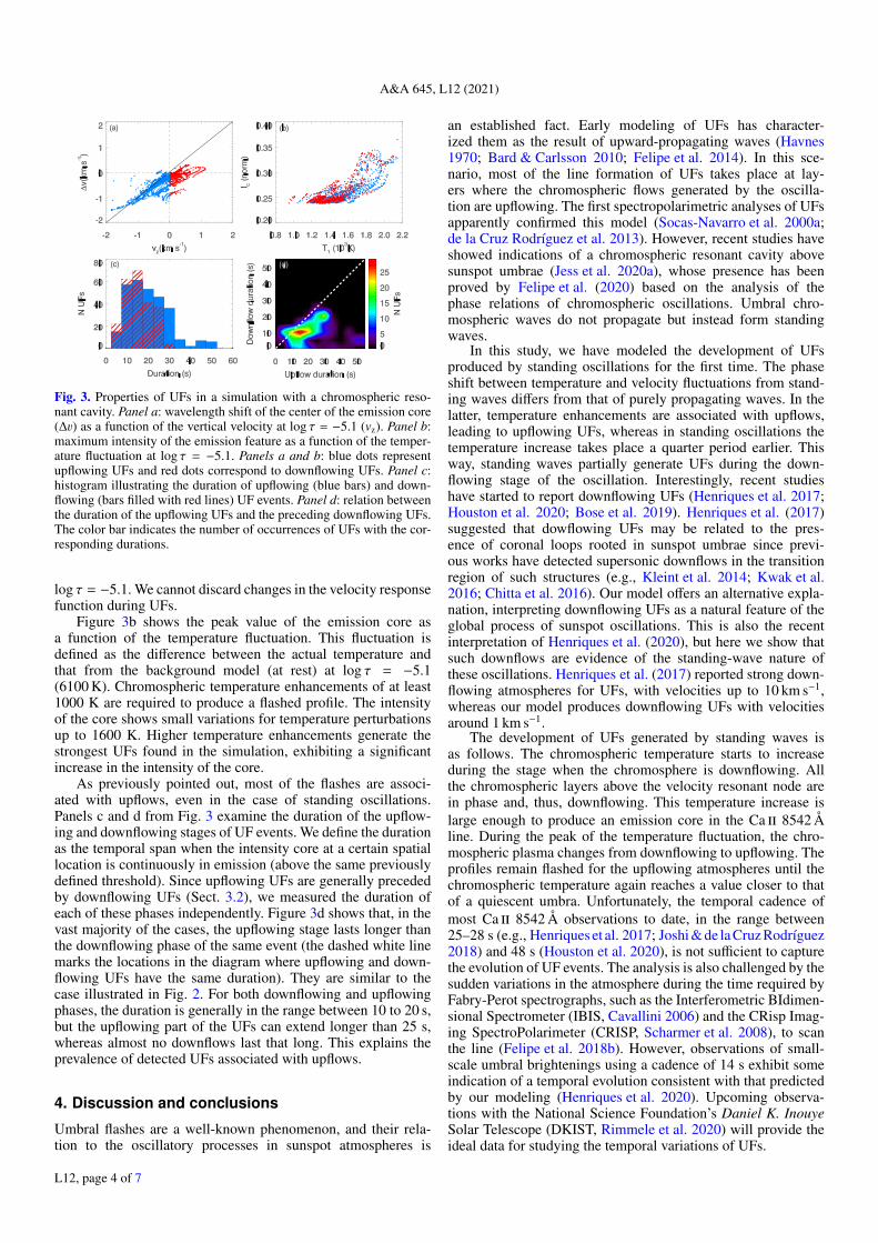
We identified a total of 1777 flashed profiles in the numericalsimulation once the standing oscillations were established (seeAppendix A). Approximately 38% of those profiles are associ-ated with downflows at log τ = −5.1, and the rest of the casesare produced during upflows.

Figure 3 illustrates some of the properties of those UFs.Panel a shows the relation between the wavelength shift of theemission feature and the actual chromospheric velocity. For mostof the UFs, the emission core is blueshifted, even when theatmosphere generating the flash is downflowing (see Fig. 2e).Henriques et al. (2017) showed how a downflowing UF can leadto an apparently blueshifted Ca ii 8542 Å emission core. Ouranalysis is based on the evaluation of the velocity at a fixed

L12, page 3 of 7

A&A 645, L12 (2021)

Fig. 3. Properties of UFs in a simulation with a chromospheric reso-nant cavity. Panel a: wavelength shift of the center of the emission core(∆v) as a function of the vertical velocity at log τ = −5.1 (vz). Panel b:maximum intensity of the emission feature as a function of the temper-ature fluctuation at log τ = −5.1. Panels a and b: blue dots representupflowing UFs and red dots correspond to downflowing UFs. Panel c:histogram illustrating the duration of upflowing (blue bars) and down-flowing (bars filled with red lines) UF events. Panel d: relation betweenthe duration of the upflowing UFs and the preceding downflowing UFs.The color bar indicates the number of occurrences of UFs with the cor-responding durations.

log τ = −5.1. We cannot discard changes in the velocity responsefunction during UFs.

Figure 3b shows the peak value of the emission core asa function of the temperature fluctuation. This fluctuation isdefined as the difference between the actual temperature andthat from the background model (at rest) at log τ = −5.1(6100 K). Chromospheric temperature enhancements of at least1000 K are required to produce a flashed profile. The intensityof the core shows small variations for temperature perturbationsup to 1600 K. Higher temperature enhancements generate thestrongest UFs found in the simulation, exhibiting a significantincrease in the intensity of the core.

As previously pointed out, most of the flashes are associ-ated with upflows, even in the case of standing oscillations.Panels c and d from Fig. 3 examine the duration of the upflow-ing and downflowing stages of UF events. We define the durationas the temporal span when the intensity core at a certain spatiallocation is continuously in emission (above the same previouslydefined threshold). Since upflowing UFs are generally precededby downflowing UFs (Sect. 3.2), we measured the duration ofeach of these phases independently. Figure 3d shows that, in thevast majority of the cases, the upflowing stage lasts longer thanthe downflowing phase of the same event (the dashed white linemarks the locations in the diagram where upflowing and down-flowing UFs have the same duration). They are similar to thecase illustrated in Fig. 2. For both downflowing and upflowingphases, the duration is generally in the range between 10 to 20 s,but the upflowing part of the UFs can extend longer than 25 s,whereas almost no downflows last that long. This explains theprevalence of detected UFs associated with upflows.

4. Discussion and conclusions

Umbral flashes are a well-known phenomenon, and their rela-tion to the oscillatory processes in sunspot atmospheres is

an established fact. Early modeling of UFs has character-ized them as the result of upward-propagating waves (Havnes1970; Bard & Carlsson 2010; Felipe et al. 2014). In this sce-nario, most of the line formation of UFs takes place at lay-ers where the chromospheric flows generated by the oscilla-tion are upflowing. The first spectropolarimetric analyses of UFsapparently confirmed this model (Socas-Navarro et al. 2000a;de la Cruz Rodríguez et al. 2013). However, recent studies haveshowed indications of a chromospheric resonant cavity abovesunspot umbrae (Jess et al. 2020a), whose presence has beenproved by Felipe et al. (2020) based on the analysis of thephase relations of chromospheric oscillations. Umbral chro-mospheric waves do not propagate but instead form standingwaves.

In this study, we have modeled the development of UFsproduced by standing oscillations for the first time. The phaseshift between temperature and velocity fluctuations from stand-ing waves differs from that of purely propagating waves. In thelatter, temperature enhancements are associated with upflows,leading to upflowing UFs, whereas in standing oscillations thetemperature increase takes place a quarter period earlier. Thisway, standing waves partially generate UFs during the down-flowing stage of the oscillation. Interestingly, recent studieshave started to report downflowing UFs (Henriques et al. 2017;Houston et al. 2020; Bose et al. 2019). Henriques et al. (2017)suggested that dowflowing UFs may be related to the pres-ence of coronal loops rooted in sunspot umbrae since previ-ous works have detected supersonic downflows in the transitionregion of such structures (e.g., Kleint et al. 2014; Kwak et al.2016; Chitta et al. 2016). Our model offers an alternative expla-nation, interpreting downflowing UFs as a natural feature of theglobal process of sunspot oscillations. This is also the recentinterpretation of Henriques et al. (2020), but here we show thatsuch downflows are evidence of the standing-wave nature ofthese oscillations. Henriques et al. (2017) reported strong down-flowing atmospheres for UFs, with velocities up to 10 km s−1,whereas our model produces downflowing UFs with velocitiesaround 1 km s−1.

The development of UFs generated by standing waves isas follows. The chromospheric temperature starts to increaseduring the stage when the chromosphere is downflowing. Allthe chromospheric layers above the velocity resonant node arein phase and, thus, downflowing. This temperature increase islarge enough to produce an emission core in the Ca ii 8542 Åline. During the peak of the temperature fluctuation, the chro-mospheric plasma changes from downflowing to upflowing. Theprofiles remain flashed for the upflowing atmospheres until thechromospheric temperature again reaches a value closer to thatof a quiescent umbra. Unfortunately, the temporal cadence ofmost Ca ii 8542 Å observations to date, in the range between25–28 s (e.g., Henriques et al. 2017; Joshi & de la Cruz Rodríguez2018) and 48 s (Houston et al. 2020), is not sufficient to capturethe evolution of UF events. The analysis is also challenged by thesudden variations in the atmosphere during the time required byFabry-Perot spectrographs, such as the Interferometric BIdimen-sional Spectrometer (IBIS, Cavallini 2006) and the CRisp Imag-ing SpectroPolarimeter (CRISP, Scharmer et al. 2008), to scanthe line (Felipe et al. 2018b). However, observations of small-scale umbral brightenings using a cadence of 14 s exhibit someindication of a temporal evolution consistent with that predictedby our modeling (Henriques et al. 2020). Upcoming observa-tions with the National Science Foundation’s Daniel K. InouyeSolar Telescope (DKIST, Rimmele et al. 2020) will provide theideal data for studying the temporal variations of UFs.

L12, page 4 of 7

T. Felipe et al.: Downflowing umbral flashes

Our simulations show that the upflowing stage of UFs isgenerally longer than the downflowing part (Fig. 3d). This isin agreement with the prevalence of upflowing solutions inNLTE inversions of observed UFs (Socas-Navarro et al. 2000a;de la Cruz Rodríguez et al. 2013), even in studies where down-flowing UFs are also reported (Houston et al. 2020).

This Letter provides a missing piece of the puzzle in what hasbeen a convergence of observations and simulations: We havetied together the evidence for downflowing UFs and the exis-tence of cavities in the chromosphere of the umbra as the latterwill naturally generate the former. Finally, the case for a corru-gated surface where downflows are significant (Henriques et al.2020), together with the importance of cavities for such down-flows, implies that future observations constraining the transitionregion of sunspots should find the transition region itself to behighly corrugated.

Acknowledgements. Financial support from the State Research Agency (AEI)of the Spanish Ministry of Science, Innovation and Universities (MCIU) andthe European Regional Development Fund (FEDER) under grant with refer-ence PGC2018-097611-A-I00 is gratefully acknowledged. VMJH is fundedby the European Research Council (ERC) under the European Union’s Hori-zon 2020 research and innovation programme (SolarALMA, grant agreementNo. 682462) and by the Research Council of Norway through its Centresof Excellence scheme (project 262622). JdlCR is supported by grants fromthe Swedish Research Council (2015-03994) and the Swedish National SpaceAgency (128/15). This project has received funding from the European ResearchCouncil (ERC) under the European Union’s Horizon 2020 research and inno-vation program (SUNMAG, grant agreement 759548). The authors wish toacknowledge the contribution of Teide High-Performance Computing facilitiesto the results of this research. TeideHPC facilities are provided by the InstitutoTecnológico y de Energías Renovables (ITER, SA). URL: http://teidehpc.iter.es.

ReferencesAl, N., Bendlin, C., & Kneer, F. 1998, A&A, 336, 743Anan, T., Schad, T. A., Jaeggli, S. A., & Tarr, L. A. 2019, ApJ, 882, 161Avrett, E. H. 1981, in The Physics of Sunspots, eds. L. E. Cram, & J. H. Thomas,

235Bard, S., & Carlsson, M. 2010, ApJ, 722, 888Beckers, J. M., & Tallant, P. E. 1969, Sol. Phys., 7, 351Berenger, J. P. 1994, J. Comput. Phys., 114, 185Bharti, L., Hirzberger, J., & Solanki, S. K. 2013, A&A, 552, L1Bose, S., Henriques, V. M. J., Rouppe van der Voort, L., & Pereira, T. M. D.

2019, A&A, 627, A46Cavallini, F. 2006, Sol. Phys., 236, 415Centeno, R., Socas-Navarro, H., Collados, M., & Trujillo Bueno, J. 2005, ApJ,

635, 670Centeno, R., Collados, M., & Trujillo Bueno, J. 2006, ApJ, 640, 1153

Chitta, L. P., Peter, H., & Young, P. R. 2016, A&A, 587, A20Christensen-Dalsgaard, J., Dappen, W., Ajukov, S. V., et al. 1996, Science, 272,

1286de la Cruz Rodríguez, J., Rouppe van der Voort, L., Socas-Navarro, H., & van

Noort, M. 2013, A&A, 556, A115Deubner, F.-L. 1974, Sol. Phys., 39, 31Felipe, T. 2019, A&A, 627, A169Felipe, T. 2021, Nat. Astron., 5, 2Felipe, T., & Esteban Pozuelo, S. 2019, A&A, 632, A75Felipe, T., Khomenko, E., Collados, M., & Beck, C. 2010a, ApJ, 722, 131Felipe, T., Khomenko, E., & Collados, M. 2010b, ApJ, 719, 357Felipe, T., Khomenko, E., & Collados, M. 2011, ApJ, 735, 65Felipe, T., Socas-Navarro, H., & Khomenko, E. 2014, ApJ, 795, 9Felipe, T., Socas-Navarro, H., & Przybylski, D. 2018a, A&A, 614, A73Felipe, T., Kuckein, C., & Thaler, I. 2018b, A&A, 617, A39Felipe, T., Kuckein, C., González Manrique, S. J., Milic, I., & Sangeetha, C. R.

2020, ApJ, 900, L29González-Morales, P. A., Khomenko, E., Downes, T. P., & de Vicente, A. 2018,

A&A, 615, A67Havnes, O. 1970, Sol. Phys., 13, 323Henriques, V. M. J., & Kiselman, D. 2013, A&A, 557, A5Henriques, V. M. J., Scullion, E., Mathioudakis, M., et al. 2015, A&A, 574, A131Henriques, V. M. J., Mathioudakis, M., Socas-Navarro, H., & de la Cruz

Rodríguez, J. 2017, ApJ, 845, 102Henriques, V. M. J., Nelson, C. J., Rouppe van der Voort, L. H. M., &

Mathioudakis, M. 2020, A&A, 642, A215Houston, S. J., Jess, D. B., Asensio Ramos, A., et al. 2018, ApJ, 860, 28Houston, S. J., Jess, D. B., Keppens, R., et al. 2020, ApJ, 892, 49Jess, D. B., Snow, B., Houston, S. J., et al. 2020a, Nat. Astron., 4, 220Jess, D. B., Snow, B., Fleck, B., Stangalini, M., & Jafarzadeh, S. 2020b, Nat.

Astron., 5, 5Joshi, J., & de la Cruz Rodríguez, J. 2018, A&A, 619, A63Khomenko, E., & Collados, M. 2006, ApJ, 653, 739Kleint, L., Antolin, P., Tian, H., et al. 2014, ApJ, 789, L42Kwak, H., Chae, J., Song, D., et al. 2016, ApJ, 821, L30Maltby, P., Avrett, E. H., Carlsson, M., et al. 1986, ApJ, 306, 284Nelson, C. J., Henriques, V. M. J., Mathioudakis, M., & Keenan, F. P. 2017,

A&A, 605, A14Rimmele, T. R., Warner, M., Keil, S. L., et al. 2020, Sol. Phys., 295, 172Rouppe van der Voort, L., & de la Cruz Rodríguez, L., 2013, ApJ. 776, 56Scharmer, G. B., Narayan, G., Hillberg, T., et al. 2008, ApJ, 689, L69Socas-Navarro, H., Trujillo Bueno, J., & Ruiz Cobo, B. 2000a, Science, 288,

1396Socas-Navarro, H., Trujillo Bueno, J., & Ruiz Cobo, B. 2000b, ApJ, 544, 1141Socas-Navarro, H., Trujillo Bueno, J., & Ruiz Cobo, B. 2001, ApJ, 550, 1102Socas-Navarro, H., McIntosh, S. W., Centeno, R., de Wijn, A. G., & Lites, B. W.

2009, ApJ, 696, 1683Socas-Navarro, H., de la Cruz Rodríguez, J., Asensio Ramos, A., Trujillo Bueno,

J., & Ruiz Cobo, B. 2015, A&A, 577, A7Wedemeyer-Böhm, S., & Carlsson, M. 2011, A&A, 528, A1Wittmann, A. 1969, Sol. Phys., 7, 366Yurchyshyn, V., Abramenko, V., Kosovichev, A., & Goode, P. 2014, ApJ, 787,

58Zhugzhda, Y. D. 2008, Sol. Phys., 251, 501Zhugzhda, Y. D., & Locans, V. 1981, Sov. Astron. Lett., 7, 25

L12, page 5 of 7

A&A 645, L12 (2021)

Appendix A: Numerical setup

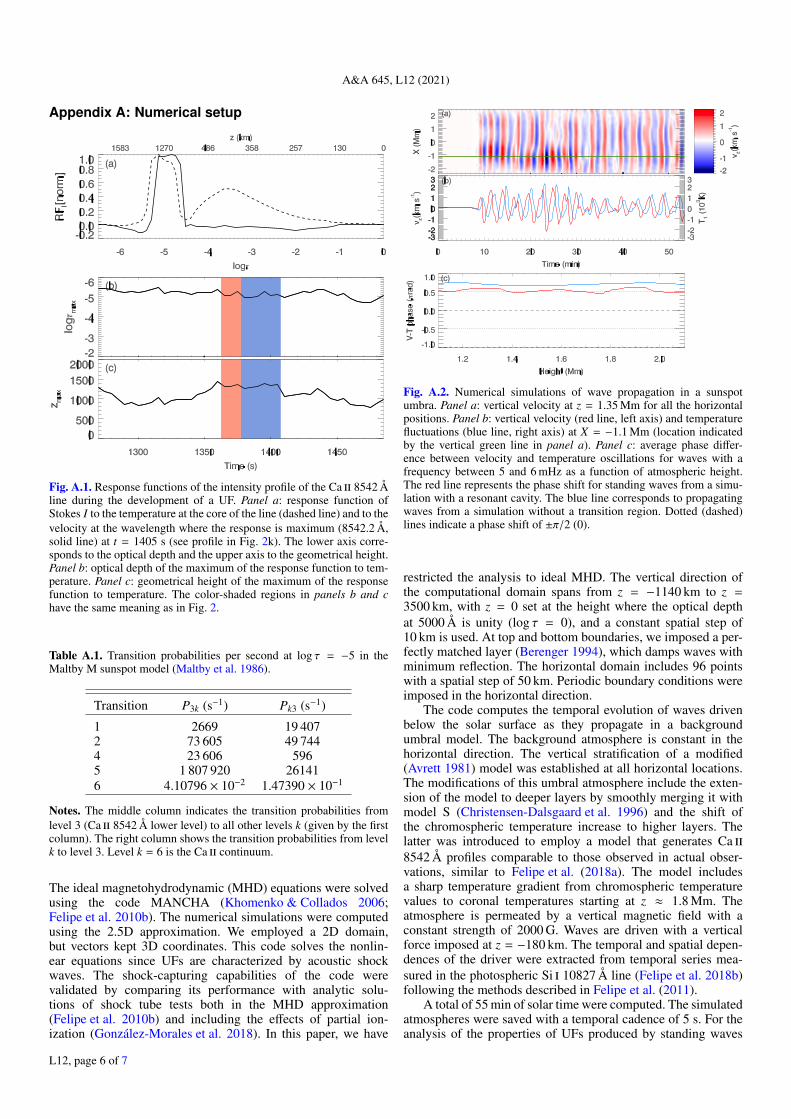
Fig. A.1. Response functions of the intensity profile of the Ca ii 8542 Åline during the development of a UF. Panel a: response function ofStokes I to the temperature at the core of the line (dashed line) and to thevelocity at the wavelength where the response is maximum (8542.2 Å,solid line) at t = 1405 s (see profile in Fig. 2k). The lower axis corre-sponds to the optical depth and the upper axis to the geometrical height.Panel b: optical depth of the maximum of the response function to tem-perature. Panel c: geometrical height of the maximum of the responsefunction to temperature. The color-shaded regions in panels b and chave the same meaning as in Fig. 2.

Table A.1. Transition probabilities per second at log τ = −5 in theMaltby M sunspot model (Maltby et al. 1986).

Transition P3k (s−1) Pk3 (s−1)

1 2669 19 4072 73 605 49 7444 23 606 5965 1 807 920 261416 4.10796 × 10−2 1.47390 × 10−1

Notes. The middle column indicates the transition probabilities fromlevel 3 (Ca ii 8542 Å lower level) to all other levels k (given by the firstcolumn). The right column shows the transition probabilities from levelk to level 3. Level k = 6 is the Ca ii continuum.

The ideal magnetohydrodynamic (MHD) equations were solvedusing the code MANCHA (Khomenko & Collados 2006;Felipe et al. 2010b). The numerical simulations were computedusing the 2.5D approximation. We employed a 2D domain,but vectors kept 3D coordinates. This code solves the nonlin-ear equations since UFs are characterized by acoustic shockwaves. The shock-capturing capabilities of the code werevalidated by comparing its performance with analytic solu-tions of shock tube tests both in the MHD approximation(Felipe et al. 2010b) and including the effects of partial ion-ization (González-Morales et al. 2018). In this paper, we have

Fig. A.2. Numerical simulations of wave propagation in a sunspotumbra. Panel a: vertical velocity at z = 1.35 Mm for all the horizontalpositions. Panel b: vertical velocity (red line, left axis) and temperaturefluctuations (blue line, right axis) at X = −1.1 Mm (location indicatedby the vertical green line in panel a). Panel c: average phase differ-ence between velocity and temperature oscillations for waves with afrequency between 5 and 6 mHz as a function of atmospheric height.The red line represents the phase shift for standing waves from a simu-lation with a resonant cavity. The blue line corresponds to propagatingwaves from a simulation without a transition region. Dotted (dashed)lines indicate a phase shift of ±π/2 (0).

restricted the analysis to ideal MHD. The vertical direction ofthe computational domain spans from z = −1140 km to z =3500 km, with z = 0 set at the height where the optical depthat 5000 Å is unity (log τ = 0), and a constant spatial step of10 km is used. At top and bottom boundaries, we imposed a per-fectly matched layer (Berenger 1994), which damps waves withminimum reflection. The horizontal domain includes 96 pointswith a spatial step of 50 km. Periodic boundary conditions wereimposed in the horizontal direction.

The code computes the temporal evolution of waves drivenbelow the solar surface as they propagate in a backgroundumbral model. The background atmosphere is constant in thehorizontal direction. The vertical stratification of a modified(Avrett 1981) model was established at all horizontal locations.The modifications of this umbral atmosphere include the exten-sion of the model to deeper layers by smoothly merging it withmodel S (Christensen-Dalsgaard et al. 1996) and the shift ofthe chromospheric temperature increase to higher layers. Thelatter was introduced to employ a model that generates Ca ii8542 Å profiles comparable to those observed in actual obser-vations, similar to Felipe et al. (2018a). The model includesa sharp temperature gradient from chromospheric temperaturevalues to coronal temperatures starting at z ≈ 1.8 Mm. Theatmosphere is permeated by a vertical magnetic field with aconstant strength of 2000 G. Waves are driven with a verticalforce imposed at z = −180 km. The temporal and spatial depen-dences of the driver were extracted from temporal series mea-sured in the photospheric Si i 10827 Å line (Felipe et al. 2018b)following the methods described in Felipe et al. (2011).

A total of 55 min of solar time were computed. The simulatedatmospheres were saved with a temporal cadence of 5 s. For theanalysis of the properties of UFs produced by standing waves

L12, page 6 of 7

T. Felipe et al.: Downflowing umbral flashes

(Sect. 3.3), we avoided the first 15 min of the simulation sinceduring this time the first wavefronts are arriving in the chromo-sphere and the standing oscillations are not established. Thus,the analysis was restricted to the last 40 min of simulations.

Appendix B: Spectral synthesis

The Stokes profiles of the Ca ii 8542 Å line were synthesized forall the spatial locations and time steps of the simulation usingthe NLTE code NICOLE (Socas-Navarro et al. 2015). NICOLEwas fed with the velocity, temperature, gas pressure, density,and magnetic field vector stratification of each atmosphere (fora specific horizontal position and time) in a geometrical scale,as given by the output of the numerical simulation. An artifi-cial macroturbulence of 1.8 km s−1 was added to compensate forthe absence of small-scale motions in the numerical calculationsand generate broader line profiles, similar to those measured inactual observations. The Stokes profiles were first synthesizedwith a spectral resolution of 5 mÅ. They were then degraded toa resolution of 55 mÅ by convolving them with a 100 mÅ fullwidth half maximum Gaussian filter centered at the wavelengthschosen for the spectral sampling.

Table A.1 shows the transition probabilities from the lowerlevel of the Ca ii 8542 Å line to all other levels and vice versa.The large values point to very short characteristic transitiontimes (below one second), confirming that the assumption of sta-tistical equilibrium leads to very small decay times, shorter thanthe temporal scales of interest for our study. The only exceptionsare the rates to and from the Ca ii continuum (k = 6). The char-acteristic times for this transition are on the order of minutes,which means that ionization to Ca iiimight be lagging behind thedynamics. However, this is not relevant for our purposes sinceCa ii is the dominant species.

Figure A.1 illustrates the response function of the Ca ii8542 Å intensity to the temperature during the development ofa UF. The main contribution to Stokes I comes from an opti-cal depth around log τ = −5.1. We chose this optical depth asthe reference for the analyses presented in this study since it ismaintained as the main contribution to the formation of the lineduring the whole temporal span of UFs (color-shaded regions inFig. A.1b). During this time, log τ = −5.1 samples a geometricalheight around z = 1350 km (Fig. A.1c). Remarkable changes inthe chromospheric region with higher sensitivity to the tempera-ture are found between flashed and non-flashed profiles (rangingbetween log τ = −4.7 and log τ = −5.6).

Appendix C: Standing and propagatingoscillations

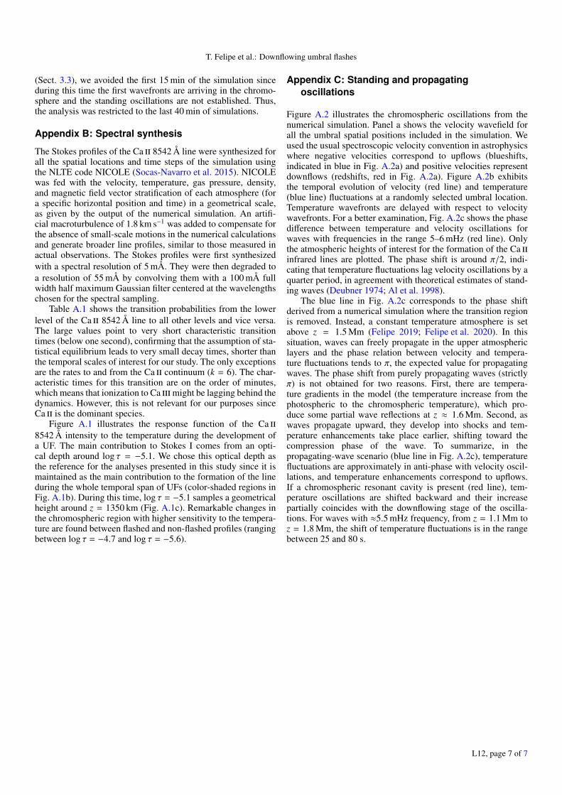
Figure A.2 illustrates the chromospheric oscillations from thenumerical simulation. Panel a shows the velocity wavefield forall the umbral spatial positions included in the simulation. Weused the usual spectroscopic velocity convention in astrophysicswhere negative velocities correspond to upflows (blueshifts,indicated in blue in Fig. A.2a) and positive velocities representdownflows (redshifts, red in Fig. A.2a). Figure A.2b exhibitsthe temporal evolution of velocity (red line) and temperature(blue line) fluctuations at a randomly selected umbral location.Temperature wavefronts are delayed with respect to velocitywavefronts. For a better examination, Fig. A.2c shows the phasedifference between temperature and velocity oscillations forwaves with frequencies in the range 5–6 mHz (red line). Onlythe atmospheric heights of interest for the formation of the Ca iiinfrared lines are plotted. The phase shift is around π/2, indi-cating that temperature fluctuations lag velocity oscillations by aquarter period, in agreement with theoretical estimates of stand-ing waves (Deubner 1974; Al et al. 1998).

The blue line in Fig. A.2c corresponds to the phase shiftderived from a numerical simulation where the transition regionis removed. Instead, a constant temperature atmosphere is setabove z = 1.5 Mm (Felipe 2019; Felipe et al. 2020). In thissituation, waves can freely propagate in the upper atmosphericlayers and the phase relation between velocity and tempera-ture fluctuations tends to π, the expected value for propagatingwaves. The phase shift from purely propagating waves (strictlyπ) is not obtained for two reasons. First, there are tempera-ture gradients in the model (the temperature increase from thephotospheric to the chromospheric temperature), which pro-duce some partial wave reflections at z ≈ 1.6 Mm. Second, aswaves propagate upward, they develop into shocks and tem-perature enhancements take place earlier, shifting toward thecompression phase of the wave. To summarize, in thepropagating-wave scenario (blue line in Fig. A.2c), temperaturefluctuations are approximately in anti-phase with velocity oscil-lations, and temperature enhancements correspond to upflows.If a chromospheric resonant cavity is present (red line), tem-perature oscillations are shifted backward and their increasepartially coincides with the downflowing stage of the oscilla-tions. For waves with ≈5.5 mHz frequency, from z = 1.1 Mm toz = 1.8 Mm, the shift of temperature fluctuations is in the rangebetween 25 and 80 s.

L12, page 7 of 7