1

Tomasz Bigaj

Counterfactuals and non-locality of quantum mechanics

Abstract

In the paper the proof of the non-locality of quantum mechanics, given recently by H. Stapp and D. Bedford, and

appealing to the GHZ example, is analyzed. The proof does not contain any explicit assumption of realism, but

instead it uses formal methods and techniques of the Lewis calculus of counterfactuals. To ascertain the validity

of the proof, a formal semantic model for counterfactuals is constructed. With the help of this model it can be

shown that the proof is faulty, because it appeals to the unwarranted principle of “Elimination of Eliminated

Conditions” (EEC). As an additional way of showing unreasonableness of the EEC assumption, it is argued that

yet another alleged and highly controversial Stapp’s proof of non-locality of QM, using the Hardy example, can

be made almost trivial with the help of EEC. Next the question is considered whether the validity of the proof in

the GHZ case can be restored by adopting the assumption of “partial realism”. It is argued that although this

assumption makes the crucial step of the original reasoning valid, it nevertheless renders another important

transition unjustified, therefore the entire reasoning collapses.

Introduction

One of the greatest achievements of the foundational analysis of quantum mechanics is

undoubtedly the Bell theorem. Although there is still a debate going on concerning particular

consequences of this theorem, it is clear that its main message is the following: there can be

no hidden-variable theory which would produce the same observational consequences as

standard quantum mechanics, and yet would be local. The structure of the original Bell

argument is well known: it proceeds from the assumption of the existence of a hidden variable

theory (or in other words from the ontological assumption of realism about values of

observables) and from the suitably formulated assumption of locality (roughly speaking, this

assumption says that a distant measurement performed on one system cannot change the

objective value of an observable pertaining to another system) to a consequence which is

incompatible with the standard quantum-mechanical predictions (this consequence is the Bell

inequality). Since the time of the original Bell argument there have been numerous attempts to

generalize or to improve it with respect to both technical details and fundamental

assumptions. Hence now we have Bell-like theorems which deal with imperfect correlations

2

or imperfect measurements, which refer to more than two separate particles, which don’t

involve any inequalities, etc.1

Without doubts, philosophically the most interesting attempts are those that aim at

weakening the crucial assumptions of the original Bell theorem. A notable example of this

kind of undertakings can be found in works of Henry P. Stapp, a physicist with a strong

philosophical motivation. Since 1971 he has published several papers in which he argues

essentially that the assumption of realism is not necessary in obtaining a contradiction with

quantum-mechanical predictions. Stapp claims that from the locality assumption alone

together with quantum-mechanical predictions a contradiction can be derived. This claim, if

justified, would constitute the strongest argument for the non-locality of quantum mechanics.2

What is particularly interesting about Stapp’s arguments is that he relies heavily on

counterfactual reasonings, i.e. reasonings concerning what would have happen, had things

been different. This fact of course can raise justified suspicions. After all, aren’t we convinced

by the founding fathers of quantum mechanics (like Bohr himself) that within quantum realms

we should talk only about what is measured, and not what could, or would be measured? This

suspicion toward counterfactuals is explicitly expressed for example by B. van Fraassen

(1991), when he says that

the violation of Bell’s inequalities demonstrates empirically that we should not look to measurement

outcomes to give us direct information about state, propensity, capacity, ability, or counterfactual facts.

From fact to modality, only the most meager inferences are allowed (p. 125, italics mine).

Yet there is a strong opposition against this “positivistic” approach to the validity of

counterfactual suppositions in quantum theory. Many physicists and philosophers point out

that whenever we talk about laws of nature (and quantum mechanics does not drop this talk at

all), we must assume some kind of “counterfactuality”: laws tell us not only what happens

actually, but first and foremost, what would happen, if the conditions were such-and-such (see

Maudlin 1994, pp. 126-32; Unruh 1999). The only problem with counterfactuals is that we

should be extremely cautious in using them. For example, as van Fraassen rightly points out,

1 For an extensive but accessible survey of different versions of Bell’s theorem, see (Placek 2000, chapter 5 “Charting the labyrinth of the Bell’s theorems”). 2 It should be stressed here that by “non-locality” Stapp means something really strong: not only that there are correlations between results of experiments on spatially separated particles (which is well known and widely accepted), but that the mere performing of measurement on one system can influence the result of the experiment on a distant system (these two types of non-locality were originally introduced in Jarrett 1984; after A. Shimony it is common to call them “outcome dependence” and “parameter dependence”).

3

we cannot take for granted some apparently plausible rules, like the rule of counterfactual

definiteness, or “counterfactual excluded middle”, which says that for any sentences A and B,

either if it were that A, then it would be B, or if it were that A, then there would be not B.

It is commonly held that the Lewis formal analysis of counterfactuals, inspired by

Stalnaker’s approach but differing from it in some crucial points, can overcome these

difficulties and be safely applied to quantum-mechanical phenomena. This is the assumption

which is made by Stapp. He claims to have used the Lewis counterfactuals in order to prove

his theorem. Actually, three different versions of his argument can be found in his writings.

The earliest version, using the original EPR-like situation from the Bell theorem, was

presented in (Stapp 1971), and then refined on different occasions (Stapp 1989). This

argument was heavily criticized by Redhead and the others (Redhead 1987, Redhead et al.

1990). Another, most recent argument, uses an example known as the Hardy experiment

(Stapp 1997). It ignited a lively discussion involving philosophically-oriented physicists

(Mermin 1998, Unruh 1999, Finkelstein 1998). And there is a third version of Stapp’s

theorem, dealing with the so-called GHZ example. This argument was originally formulated

in (Stapp 1991) and then refined and formalized in (Bedford, Stapp 1995) with explicit

reference to the Lewis calculus of counterfactuals.

The GHZ version of Stapp’s argument, especially in its version from 1995, is

definitely the most advanced with respect to logical details. Maybe for that reason it has not

received much attention from physicists and philosophers, and has passed virtually

unchallenged. Yet it appears that in spite of its meticulous presentation with respect to almost

every technical detail, Stapp’s proof3 contains serious flaws which make the conclusion

unjustified. In what follows, I would like to present a detailed analysis of this proof, which

can serve different purposes. First of all it will clarify somewhat obscure steps of the

argument, by pointing out that this argument is a counterfactual version of a much simpler

argument which can be made when the assumption of realism is invoked, much as in the

original Bell theorem. But most importantly, my analysis is going to show where exactly

Stapp’s argument fails, and why his conclusion is unwarranted. I will also raise the question

whether the argument can be corrected by adding an additional assumption which I call

“partial realism”. It will turn out that in spite of its initial plausibility, even this partial realism

cannot produce the needed results. As far as the technical aspect of my article is concerned, I

am going to introduce certain semantic tools for assessing validity of logical transitions within

3 With all required credits for the second co-author, D. Bedford, I will call the analyzed argument for short “Stapp’s argument” throughout the paper.

4

Stapp’s alleged proof. These tools will be essentially Lewis-style possible-world semantic

models for counterfactuals, tailored to the physical situation in question.

1. Initial assumptions

The original proof deals with an example of the Greenberger–Horne–Zeilinger (GHZ)

situation in its version with three particles. I will not go here into the physical details

concerning this example (for a physical presentation see Greenberger et al. 1990; Auletta

2000, pp. 628-33). The only thing we should know is that there are three particles 1, 2, 3, and

each of them can undergo one of two measurements Xi or Yi, with two possible results each: xi

= +1 or –1 and yi = +1 or –1. When these three particles are prepared in a special initial state,

there are certain correlations between possible results of the above-mentioned measurements.

These correlations can be presented as follows:

(QM1) X1X2X3 ⇒ x1x2x3 = –1

(QM2) X1Y2Y3 ⇒ x1y2y3 = +1

(QM3) Y1X2Y3 ⇒ y1x2y3 = +1

(QM4) Y1Y2X3 ⇒ y1y2x3 = +1

In words (QM1–4) says that when the measurements X1, X2, and X3 are jointly

performed, the product of their results must equal –1, and with the other three combinations

the product is positive. It is important to stress that these correlations take place even if

measurements are space-like separated from each other, so that no known physical interaction

can appear between all particles.

Now, it is quite obvious that the above predictions lead to a contradiction when we

assume that each observable in question has its objective value independently of the

measurement revealing it, and independently of the two other measurements – in other words,

that all numbers xi and yi have determinate values. To prove this, it suffices to multiply all

sides of the equations (QM1-4). On the right-hand side we will obtain the product –1, but on

the left-hand side each particular value will be squared, and therefore their total product must

equal 1.

Here we have repeated the usual Bell result that realism plus locality is incompatible

with standard formalism of QM. However, Stapp claims that with the help of this GHZ

example we can prove even more: without assuming realism, only using counterfactual

5

reasonings about possible experiments and assuming some version of locality, he wants to

show that a contradiction can be derived from (QM1–4). Actually, his proof of this

contradiction, both in the earlier and in the refined version, consists of a quite complicated

and not necessarily intuitive chain of derivations. But we can make it a little bit more

accessible by pointing out that this proof essentially mimics one of several possible ways of

deriving a contradiction in the easier case of realism. However, this is not the way we have

just presented. Obviously, the reasoning sketched above requires multiplication of six

different results of experiments, and we cannot hope to reproduce this in counterfactual

reasoning. We should rather find such a way of proceeding that at each step only a minimal

number of different values is invoked. And here is one such possible way of reasoning.

We start, as before, with the assumptions (QM1) and (QM2), noting the following

implication:

(R1) x2x3 = –p ⇒ y2y3 = p

This implication goes through, because we assume the existence of the objective value of x1.

In the same way we can proceed from (QM3) and (QM4):

(R2) y2x3 = q ⇒ x2y3 = q

And now suppose that three observables X2, X3 and Y2 have the following values: x2 = m, x3 =

n, and y2 = r. Then by (R1) we have y2y3 = –mn, and hence

(R3) x2 = m ∧ x3 = n ∧ y2 = r ⇒ y3 = –mnr

But from (R2), which is true for all q, we can obviously infer that x2y3 = rn, which means,

given (R3), that x2 = –m. Here we have ended up with a contradiction: from the assumption

that x2 = m we have derived that x2 = –m.

Now we can at least hope to find counterfactual representations for each step in this

reasoning. For example step (R1) could be presented as follows: if we measured X1, X2, X3,

and obtained x2x3 = p, then if we had chosen Y2Y3 instead of X2X3, we would have obtained

y2y3 = –p. However, the proof of this counterfactual counterpart will turn out to be somewhat

intricate, to put it mildly.

6

Stapp obviously must rely on some assumptions. His main premise is the assumption

of locality, interpreted with the help of counterfactual conditionals. It says roughly that when

we change counterfactually one or two of the measured observables, the result obtained in the

third measurement should not change. We will take this assumption for granted, although it

was heavily criticized in the context of another of Stapp’s arguments by Redhead4. Then there

is an entire battery of valid patterns of inference in the Lewis counterfactual calculus, whose

validity Bedford and Stapp establish scrupulously in (1995). And the third component of

Stapp’s auxiliary premises consists of two patterns of inference, which although not generally

valid in the Lewis calculus, are claimed to be valid in the particular context of the GHZ

example. The first rule is called “Elimination of Eliminated Conditions” (note the tautological

character of this nomenclature); the second has no name, but it can be called “Addition of

Irrelevant Conditions”. I will formulate them later, when they are needed. Not surprisingly, it

will appear that one of them is essentially responsible for the failure of the entire reasoning.

The first step in the proof aims at showing the validity of the counterfactual analogue

of the thesis (R1):

(C1) X2X3 ∧ x2x3 = –p ⇒ (Y2Y3 → y2y3 = p)

It appears that this is not such an easy task. First, we will have, following Stapp, to appeal to

the locality assumption:

(LOC1) X1X2X3 ∧ x1 = p ⇒ (X1Y2Y3 → x1 = p)

In words: if we obtain the result x1 = p, while choosing for the other two particles

measurements X2 and X3, then this result should be valid even if we counterfactually chose Y2

and Y3. Now, when we appeal to the predictions (QM1) and (QM2), we can easily convince

ourselves that the following must hold:

(1) X1X2X3 ∧ x2x3 = –p ⇒ (X1Y2Y3 → y2y3 = p)

4 The essential point of disagreement between Stapp and Redhead lies in a different way of reading counterfactuals with antecedents referring to a localized spatiotemporal event. Stapp implicitly assumes that in order to evaluate such a counterfactual we should analyze all possible worlds which are the same as the actual one with respect to the whole space-time region outside the absolute future of the event, whereas Redhead claims that what should be kept fixed is confined only to the absolute past of this event. I have analyzed this distinction extensively elsewhere (Bigaj 2002a, 2002b).

7

But (1) still falls short of the needed (C1). In (1) the counterfactual argument from x2x3 = –p

to y2y3 goes through only in virtue of the measurement X1 being an “intermediate” element.

But we need something stronger: no matter what measurement is performed on the particle 1,

as long as x2x3 = –p, the results of the would-be measurements Y2 and Y3 must obey the

equation y2y3 = p. And here Stapp tries the following route: suppose that the actual

measurement performed on the particle 1 is Y1. In virtue of the locality assumption we can

argue for the following:

(LOC1′) Y1X2X3 ∧ x2x3 = –p ⇒ (X1X2X3 → x2x3 = –p)

Now we can proceed using the already proven (1), and replacing the consequent of the

counterfactual by the consequent of (1) (this move is in agreement with the Lewis rules of

inference):

(2) Y1X2X3 ∧ x2x3 = –p ⇒ (X1X2X3 → (X1Y2Y3 → y2y3 = p)).

And in order to return to the situation when Y1Y2Y3 are performed, we can still appeal to the

locality condition, arguing that the equation y2y3 = p should remain unchanged. Hence we

obtain the following chain of counterfactuals:

(3) Y1X2X3 ∧ x2x3 = –p ⇒ (X1X2X3 → (X1Y2Y3 → (Y1Y2Y3 → y2y3 = p))).

We can see that the first and the last elements of this chain are exactly the ones we

need to get, if we want to obtain a version of (1) with the measurement Y1 instead of X1. But

how to get rid of the intermediate elements (intermediate counterfactual situations)? Here

Stapp appeals to the earlier announced principle of the “Elimination of Eliminated

Conditions”. Essentially, he would claim that each counterfactual supposition in (3) annuls

the preceding one, so we are finally left with the last only. This may look convincing at first

sight, but let us look closer. First consider the implication (2) and ask if we are allowed to

cross out from it the counterfactual condition X1X2X3. This might seem difficult to answer,

because “double counterfactuals” are quite non-intuitive. But we can restate (2) in terms of

possible worlds, keeping in mind the ordinary truth-conditions for counterfactuals as imposed

8

by Lewis. Let w0 be the “actual” world, i.e. the world in which Y1X2X3 are performed, and the

product x2x3 equals –p. Let w1 represent the world closest to the actual, in which X1X2X3 are

performed. This is the world in which x2x3 still equals –p, and therefore by (QM1) x1 = p.

Now, in order for (2) to be true, the counterfactual X1Y2Y3 → y2y3 = p must be true at w1.

This, on the other hand, means that when we take the world w2 closest to w1 and such that

X1Y2Y3 holds, then in this world the consequent y2y3 = p should hold. Because w2 is closest to

w1, x1 should be the same as at w1, therefore at w2 x1 = p and by (QM2) we have y2y3 = p. In

that way we can argue that (2) is indeed true, if we assume the ordinary truth-conditions for

counterfactuals, together with some reasonable rules for comparing similarity between

possible worlds.

2. Semantic models for counterfactuals

Because things are getting here quite complicated, and because we will have to assess

validity of certain “non-intuitive” transformations, it would be a good idea to proceed slightly

more formally. Stapp’s entire argument relies on the standard Lewis truth-conditions of

counterfactuals and on some rules of comparative similarity between possible worlds (see

Lewis 1973, 1986). Therefore we can now formally construct a semantic model, consisting of

a set of possible worlds and of some rules defining the relation of comparative similarity

between these worlds. These rules will be incomplete, for reason which will become clear

soon, but sufficient for the valuations of all of Stapp’s transformations. Let us first start with

the definition of the set of possible worlds. In our case of the GHZ example a given possible

world is fully defined by specifying three measurements and their results. Therefore we will

formally represent a possible world by a sextuple ⟨Z1, Z2, Z3, z1, z2, z3⟩, where Zi = Xi or Yi and

zi = +1 or –1. In general, the experimental situation allows for 26 = 64 different possible

worlds, but because of the restrictions QM1–4 we have in fact 16 worlds less, therefore the

final number of possible worlds is 48.

Now we have to introduce some rules of comparative similarity. Let w0 = ⟨Z10, Z2

0, Z30,

z10, z2

0, z30⟩ be the actual world, and let w1 = ⟨Z1

1, Z21, Z3

1, z11, z2

1, z31⟩ and w2 = ⟨Z1

2, Z22, Z3

2,

z12, z2

2, z32⟩ be two possible worlds. In comparing w1 and w2 with respect to their closeness to

w0, we should take into account both the measurements performed and the results obtained.

Let us define Z10 = {Zi1: Zi

1 = Zi0}, i.e. Z10 is a set of measurements performed in the world w1,

9

which are the same as in the actual one. Analogously, Z20 = {Zi2: Zi

2 = Zi0}. The first partial

rule of comparative similarity, suggested by Stapp’s remarks, will be the following:

(CS1) If the number of elements in Z10 is no less than in Z20, then if the number of

measurements in Z10 with the same result as in w0 is greater than the number of

measurements in Z20 with the same results as in w0, then w1 <0 w2.

The expression “w1 <0 w2” is an abbreviation for “w1 is closer to w0 than w2”. The rule (CS1)

says that the number of the measurements with the same results as in the actual world counts

towards similarity, provided that the number of repeated measurements is not decreased.

(CS1) already implies Stapp’s version of the locality assumption, because according to it we

should always judge as closer to reality the world in which the result of an unchanged

measurement is the same, even if the other measurements had been chosen different.

The second rule shows that in some cases the mere difference in numbers of the same

measurements as in the actual world can count towards similarity.

(CS2) If the number of measurements in Z10 with the same result as in w0 is no less than the

number of measurements in Z20 with the same result as in w0, then if the number of

elements in Z10 is greater than the number of elements in Z20, then w1 <0 w2.

(CS2) implies another version of the locality assumption; namely that when we change some

measurement settings, the remaining settings should be unchanged. We can also add the third

rule of comparative similarity to the effect that the only situation in which we are allowed to

assert w1 <0 w2 is when the number of repeated measurements or the number of repeated

measurements with the same results is greater in w1 than in w2.

(CS3) If w1 <0 w2, then either the number of elements in Z10 is greater than the number of

elements in Z20, or the number of measurements in Z10 with the same result as in w0 is

greater than the number of measurements in Z20 with the same results as in w0.

A consequence of (CS3) is that the results of counterfactually altered measurements do not by

themselves count towards similarity, which seems reasonable.

10

It should be quite obvious that rules (CS1-3) are not sufficient to determine in each

case whether one world is closer to the actual than the other. Namely, the rules presented

above don’t decide what is more important for comparative similarity: the number of repeated

results, or the number of repeated measurements. For example, when the actual world is the

following: w0 = ⟨X1, X2, Y3, –1, –1, –1⟩, then our rules of comparative similarity cannot help in

assessing which world is closer to w0: w1 = ⟨X1, X2, X3, +1, +1, –1⟩, or w2 = ⟨Y1, Y2, Y3, +1, –1,

–1⟩. In w1 two of three measurements are the same as in w0, but none of them with the same

result; in w2 the number of repeated measurements is lesser, namely one, but the result of this

repeated measurement is the same as in w0. But (CS1) and (CS2) are completely sufficient to

evaluate the entire reasoning presented by Stapp.5

Because our universe consists of finitely many possible worlds, we can use the

following, simpler version of the Lewis truth conditions for counterfactuals:

(TC) The counterfactual A → B is true at the world w0 iff B is true at all A-worlds closest

to w0.

Let us apply this semantic model to asses again the validity of the statement (2). The strict

implication is true if its consequent is true at all possible worlds fulfilling the antecedent. In

other worlds: the counterfactual X1X2X3 → (X1Y2Y3 → y2y3 = p) must be true at all

following worlds: ⟨Y1, X2, X3, _, p, –p⟩, ⟨Y1, X2, X3, _, –p, p⟩, where “_” stands for any possible

result. That means, according to the rule (CS1), that in every world of the type ⟨X1, X2, X3, _,

p, –p⟩ or ⟨X1, X2, X3, _, –p, p⟩, the sentence (X1Y2Y3 → y2y3 = p) must hold. But because of

the quantum-mechanical prediction QM1, the blank in the result of the X1-measurement

should be replaced by p. Therefore, again according to (CS1), the closest X1Y2Y3-worlds to

these worlds are the following: ⟨X1, Y2, Y3, p, _, _⟩. But again using the quantum-mechanical

prediction QM2 we see that the product of the two blanks must equal p, and therefore the

validity of (2) is proven.

5 One possible way of dealing with this situation is to admit that some possible worlds are not comparable at all. As a consequence, the relation of comparative similarity would be no longer a linear ordering, but only a partial ordering. To see that this might be the case, observe that we cannot for example pronounce the worlds w1 and w2 as equisimilar, and by this assure fulfillment of the requirement of the connectivity. For in that case we could introduce a world w3 = ⟨X1, X2, Y3, +1, +1, +1⟩, which by the same assumption should be equally similar to w2, and yet according to (CS2) w3 > w1, which leads to a contradiction. A similar argument in favor of the thesis that in the relativistic context comparative similarity must be a partial ordering is formulated in (Finkelstein 1999). For the consequences of this thesis for the truth-conditions of counterfactuals see (Bigaj 2002b).

11

But what about the validity of (2) with X1X2X3 crossed out? Let us write it down:

(4) Y1X2X3 ∧ x2x3 = –p ⇒ (X1Y2Y3 → y2y3 = p)

Now the truth-conditions imply the following: if (4) were to be true, y2y3 = p must hold at all

the worlds ⟨X1, Y2, Y3, _, _, _⟩ which are closest to some of the worlds ⟨Y1, X2, X3, _, –p, p⟩ or

⟨Y1, X2, X3, _, p, –p⟩. But because no measurement in the former is the same as in the latter,

according to (CS3) we can impose no condition on what the results of the measurements

X1Y2Y3 should be in ⟨X1, Y2, Y3, _, _, _⟩ that are closest to some “actual” world. Therefore

there will be one such a world in which y2y3 will not be equal to p, and hence counterfactual

(4) will come out false. The transition from (2) to (4) is definitely not valid.

The rule of the “Elimination of Eliminated Conditions” cannot be taken for granted.

Stapp formulates it in the following way: if M1, M2 and M3 are three alternative triplets of

measurements, ϕ is a possible outcome of M1 and P(ϕ) is a proposition that “depends only on

ϕ”, then the following pattern of inference is valid:

(EEC) If M1 ⇒ (M2 → (M3 → P(ϕ))), then M1 ⇒ (M3 → P(ϕ))

I don’t know what the phrase “depends only on ϕ” exactly means. It could mean that P refers

only to the result of the measurement of M1, but this would be unreasonable, because the

antecedent of the last counterfactual assumes M3, not M1. And besides, in the application

leading from (2) to (4), the sentence y2y3 = p definitely does not refer to the result of the actual

measurement. For that reason I will ignore this restriction on P. And now we can see that

(EEC) is unwarranted. The counterfactual assumption M2 may introduce some new elements

to the whole situation, which together with another counterfactual assumption M3 can lead to

P, but nonetheless P will not follow from the counterfactual assumption M2 alone. It seems to

me that Stapp overlooked the fact that the “annulment” of the assumption M2 by M3 is not

total – we assume that some of our choices are different, but some remain the same, and in

virtue of the meaning of counterfactuals we have to leave intact as many facts as possible

from the world in which M3 holds.

In the conditional (2) the element which guarantees the truth of the consequent is of

course the result of the measurement X1. And now it can be conjectured that in claiming the

validity of the move from (2) to (4), Stapp implicitly assumes the objective reality of the value

12

x1, in spite of the fact that no measurement was performed to reveal this value. This

observation can serve as a possible explanation of why Stapp was able to derive a

contradiction: he apparently included some residual form of reality assumption, at least with

respect to the non-measured observable X1. But it will appear later that even under this

assumption of “partial realism” Stapp’s final conclusion is unwarranted.

3. A Hardy-type experiment

In order to see how powerful and therefore unwarranted the assumption (EEC) is, let

us observe that with the help of it another proof of non-locality by Stapp (1997) can be made

almost trivial. This proof concerns a Hardy-type experiment with two particles L and R,

mentioned earlier. I will present here the self-explanatory diagram, together with some

clarifying remarks.

R1

R2

L1

L2

d

c

a

b

e

f

g

h

Fig. 1. Quantum-mechanical predictions concerning the Hardy experiment. Solid arrows indicate strict

implications, dashed arrows indicate “possibility”. For example, the arrow leading from the result b of the

experiment L1 to the result g of the experiment R2 shows that when L1 is performed and the result obtained is b,

the result of R2 must be g. Dashed arrows leading from b to e and f indicate that when L1 gives b, both results of

the measurement R1 have non-zero probability.

And now I argue that the following chain of counterfactual reasonings must be true:

(H1) L1 ∧ b ∧ R2 ⇒ (L2 ∧ R2 → L2 ∧ R2 ∧ c) (by QM predictions and Stapp-locality

LOC1)

13

(H2) L2 ∧ c ∧ R2 ⇒ (L2 ∧ R1 → L2 ∧ R1 ∧ f) (by the same as above)

(H3) L2 ∧ R1 ∧ f ⇒ (L1 ∧ R1 → f) (by the locality alone)

Combining these three together we obtain

(H4) L1 ∧ b ∧ R2 ⇒ (L2 ∧ R2 → (L2 ∧ R1 → (L1 ∧ R1 → f)))

By appealing to (EEC) we could get rid of the intermediate elements, thus being left with

(H5) L1 ∧ b ∧ R2 ⇒ (L1 ∧ R1 → f)

This is exactly step (6) in the original Stapp proof. From this we can obtain a contradiction

with predictions of QM either, as Stapp did it, by postulating yet another version of locality,

or, as I suggested elsewhere, by appropriately rewriting QM predictions in terms of

counterfactuals. But the original path leading to (H5) was not at all straightforward, and it

required the highly suspicious assumption LOC2, contested by all subsequent critics.6 On the

other hand, here we have an intuitive, almost trivial line of argument, and the only help is

taken from (EEC). If (EEC) were a reasonable assumption, Stapp wouldn’t have to take the

route he originally took in (1997).

But let us return to the current GHZ-type argument. Now it should be obvious that the

entire argument collapses, as the chain leading to the sentence Y1X2X3 ∧ x2x3 = –p ⇒ (Y1Y2Y3

→ y2y3 = p) is broken. But in spite of this let us continue analyzing the rest of the argument.

So we will take it for granted that you can derive (4) from (2). Interestingly enough, the

elimination of the next “intermediate” counterfactual condition in (3) is perfectly acceptable.

Let us see why. We should be able to get from

(5) Y1X2X3 ∧ x2x3 = –p ⇒ (X1Y2Y3 → (Y1Y2Y3 → y2y3 = p))

to

6 Elsewhere I have shown that both assumption LOC1 and LOC2, used in the Hardy-type argument, cannot be satisfied jointly under any intuitive reading for spatiotemporal counterfactuals. A similar point is made in (Finkelstein 1998).

14

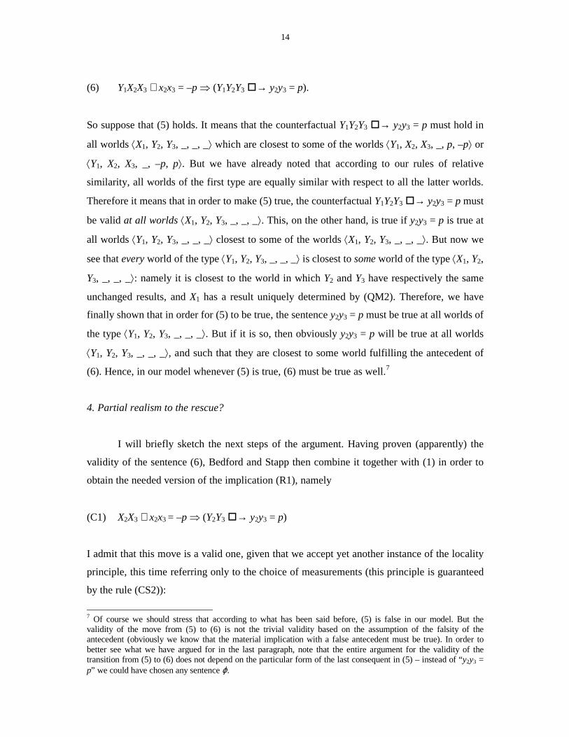
(6) Y1X2X3 ∧ x2x3 = –p ⇒ (Y1Y2Y3 → y2y3 = p).

So suppose that (5) holds. It means that the counterfactual Y1Y2Y3 → y2y3 = p must hold in

all worlds ⟨X1, Y2, Y3, _, _, _⟩ which are closest to some of the worlds ⟨Y1, X2, X3, _, p, –p⟩ or

⟨Y1, X2, X3, _, –p, p⟩. But we have already noted that according to our rules of relative

similarity, all worlds of the first type are equally similar with respect to all the latter worlds.

Therefore it means that in order to make (5) true, the counterfactual Y1Y2Y3 → y2y3 = p must

be valid at all worlds ⟨X1, Y2, Y3, _, _, _⟩. This, on the other hand, is true if y2y3 = p is true at

all worlds ⟨Y1, Y2, Y3, _, _, _⟩ closest to some of the worlds ⟨X1, Y2, Y3, _, _, _⟩. But now we

see that every world of the type ⟨Y1, Y2, Y3, _, _, _⟩ is closest to some world of the type ⟨X1, Y2,

Y3, _, _, _⟩: namely it is closest to the world in which Y2 and Y3 have respectively the same

unchanged results, and X1 has a result uniquely determined by (QM2). Therefore, we have

finally shown that in order for (5) to be true, the sentence y2y3 = p must be true at all worlds of

the type ⟨Y1, Y2, Y3, _, _, _⟩. But if it is so, then obviously y2y3 = p will be true at all worlds

⟨Y1, Y2, Y3, _, _, _⟩, and such that they are closest to some world fulfilling the antecedent of

(6). Hence, in our model whenever (5) is true, (6) must be true as well.7

4. Partial realism to the rescue?

I will briefly sketch the next steps of the argument. Having proven (apparently) the

validity of the sentence (6), Bedford and Stapp then combine it together with (1) in order to

obtain the needed version of the implication (R1), namely

(C1) X2X3 ∧ x2x3 = –p ⇒ (Y2Y3 → y2y3 = p)

I admit that this move is a valid one, given that we accept yet another instance of the locality

principle, this time referring only to the choice of measurements (this principle is guaranteed

by the rule (CS2)):

7 Of course we should stress that according to what has been said before, (5) is false in our model. But the validity of the move from (5) to (6) is not the trivial validity based on the assumption of the falsity of the antecedent (obviously we know that the material implication with a false antecedent must be true). In order to better see what we have argued for in the last paragraph, note that the entire argument for the validity of the transition from (5) to (6) does not depend on the particular form of the last consequent in (5) – instead of “y2y3 = p” we could have chosen any sentence ϕ.

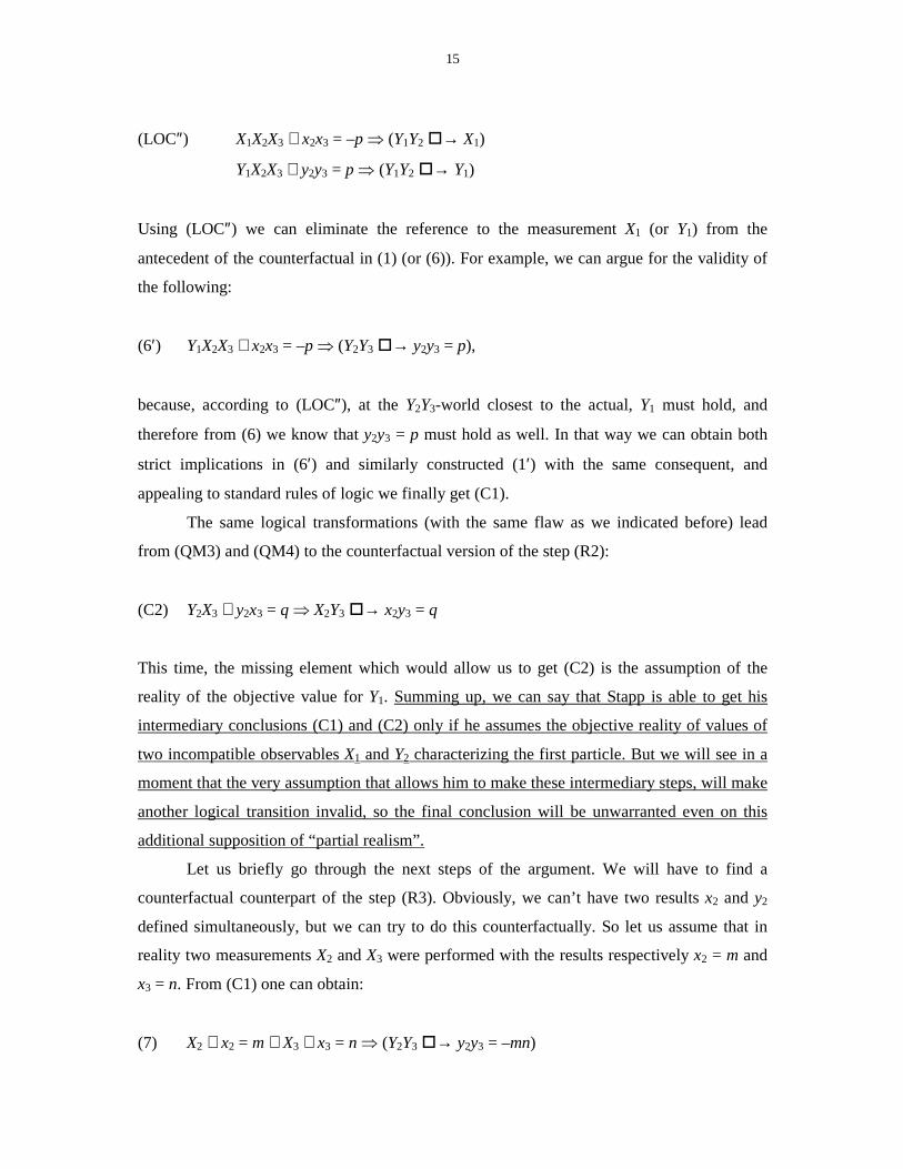
15

(LOC″) X1X2X3 ∧ x2x3 = –p ⇒ (Y1Y2 → X1)

Y1X2X3 ∧ y2y3 = p ⇒ (Y1Y2 → Y1)

Using (LOC″) we can eliminate the reference to the measurement X1 (or Y1) from the

antecedent of the counterfactual in (1) (or (6)). For example, we can argue for the validity of

the following:

(6′) Y1X2X3 ∧ x2x3 = –p ⇒ (Y2Y3 → y2y3 = p),

because, according to (LOC″), at the Y2Y3-world closest to the actual, Y1 must hold, and

therefore from (6) we know that y2y3 = p must hold as well. In that way we can obtain both

strict implications in (6′) and similarly constructed (1′) with the same consequent, and

appealing to standard rules of logic we finally get (C1).

The same logical transformations (with the same flaw as we indicated before) lead

from (QM3) and (QM4) to the counterfactual version of the step (R2):

(C2) Y2X3 ∧ y2x3 = q ⇒ X2Y3 → x2y3 = q

This time, the missing element which would allow us to get (C2) is the assumption of the

reality of the objective value for Y1. Summing up, we can say that Stapp is able to get his

intermediary conclusions (C1) and (C2) only if he assumes the objective reality of values of

two incompatible observables X1 and Y2 characterizing the first particle. But we will see in a

moment that the very assumption that allows him to make these intermediary steps, will make

another logical transition invalid, so the final conclusion will be unwarranted even on this

additional supposition of “partial realism”.

Let us briefly go through the next steps of the argument. We will have to find a

counterfactual counterpart of the step (R3). Obviously, we can’t have two results x2 and y2

defined simultaneously, but we can try to do this counterfactually. So let us assume that in

reality two measurements X2 and X3 were performed with the results respectively x2 = m and

x3 = n. From (C1) one can obtain:

(7) X2 ∧ x2 = m ∧ X3 ∧ x3 = n ⇒ (Y2Y3 → y2y3 = –mn)

16

In order to obtain the equation y3 = –mnr figuring in (R3), we must assume counterfactually

that the result of the measurement of Y2 was y2 = r. Stapp inserts this supposition between the

strict implication and the counterfactual conditional, in the form of yet another counterfactual:

(8) X2 ∧ x2 = m ∧ X3 ∧ x3 = n ⇒ (Y2 ∧ y2 = r ∧ X3 → (Y2Y3 → y3 = –mnr))

The crucial question is what justifies the move from (7) to (8). And here Stapp appeals to his

second pattern of inference, which we have dubbed “the Principle of Addition of Irrelevant

Conditions” (AIC). It essentially claims that when (7) is true, the following must be also true:

(9) X2 ∧ x2 = m ∧ X3 ∧ x3 = n ⇒ (Y2X3 → (Y2Y3 → y2y3 = –mn))

The transition from (9) to (8) is just a matter of using some unquestionable logical rules

together with simple algebra, although its proper formalization can be tedious. But this is not

a crux of the step from (7) to (8). The focal point is, of course, the principle (AIC). However,

it appears that in this context the principle (AIC) is OK, although we should stress that

generally the Lewis calculus of counterfactuals does not allow for such “insertions”. I will not

show right now that within our general semantic framework the move from (7) to (9) is valid,

leaving it to the reader. In a nutshell, the only thing we must do is to show that all Y2Y3-worlds

which are closest to some “actual” worlds (where actuality is of course understood according

to what is said in the antecedent of the strict implication in (7)), will also be closest to these

Y2X3-worlds which are closest to actuality.

The next few “logical twists and turns”, with which I have no quarrel, lead from (9)

via (C2) to the following chain of counterfactuals:

(10) X2 ∧ x2 = m ∧ X3 ⇒ (Y2X3 → (Y2Y3 → (X2Y3 → x2 = –m)))

And now the final goal seems to be within our reach: we should only get rid of these nasty

intermediate counterfactuals in order to obtain something which looks almost like a

contradiction:

(11) X2 ∧ x2 = m ∧ X3 ⇒ (X2Y3 → x2 = –m)

17

Actually, (11) contradicts our initial assumption of locality, which implies that changing

counterfactually the observable X3 for Y3 should not change the result obtained in the

measurement of X2. So the only thing we should consider right now is how to justify the step

from (10) to (11). In order to do this, we should not rely uncritically on the assumption (EEC),

for we already know that this principle is not universally valid. Instead, we can again resort to

our formal semantic model and ask if the truth of (10) can guarantee the truth of (11). Let us

then symbolize the last counterfactual X2Y3 → x2 = –m in (10) by ϕ. If (10) is to be true, ϕ

must be true in all Y2Y3-worlds which are closest to some Y2X3-worlds, which in turn must be

closest to some of the worlds allowed by the antecedent of the strict implication.

Consider then first all worlds of the type ⟨_, Y2, X3, _, _, _⟩, and ask which of them are

closest to some world of the type ⟨_, X2, X3, _, m, _⟩, which is the type defined by the

antecedent of the strict conditional in (10). In other words, we are asking what restrictions on

possible Y2X3-worlds are put by the fact that we are considering only actual worlds satisfying

the antecedent of the strict conditional. It appears that these restrictions are very mild. The

only Y2X3-worlds for which we can find no world of the type ⟨_, X2, X3, _, m, _⟩ such that the

former is closest to the latter, are the worlds of the type ⟨X1, Y2, X3, x1, y2, x3⟩, where x1x3 = m.

It is so because the worlds of the type ⟨X1, X2, X3, x1, m, x3⟩, under supposition x1x3 = m are

forbidden by requirement (QM1). For all other Y2X3-worlds one can always find a world of

the type ⟨_, X2, X3, _, m, _⟩ to which it is closest, by putting in blanks the same elements as in

the original one. This means that for (10) to be true, ϕ must be true in all Y2Y3-worlds such

that there is an Y2X3-world fulfilling the above requirement, to which our Y2Y3-world is

closest. But now it is obvious that we can find such a world of the type ⟨_, Y2, X3, _, _, _⟩ for

all Y2Y3-worlds with no exception. To do this we should only replace the first blank by the

measurement done in our initial Y2Y3-world, and insert in the next two blanks the results

obtained in this world as well, completing the entire world by inserting a result for the

measurement X3 which agrees with quantum-mechanical predictions (QM1-4). Therefore it

finally turns out that in order for (10) to be true, ϕ must be true at all Y2Y3-worlds, which

allows us to cross out Y2X3 from (10) and to obtain:

(12) X2 ∧ x2 = m ∧ X3 ⇒ (Y2Y3 → (X2Y3 → x2 = –m))).

18

The same reasoning can convince us that in order for (12) to be true, the sentence x2 = –m

should be true at all X2Y3-worlds. Therefore, we can finally achieve (11) as our ultimate result.

To recapitulate: Stapp’s entire reasoning appeared to be valid within our semantic

model, with a notable exception of one crucial step, leading from (2) to (4); therefore the

arguments fails. The purported non-locality of QM turns out to be unwarranted. However, one

interesting thing remains to be analyzed. We remarked earlier that the minimal condition

which would make the questioned move valid requires that both X1 and Y1 have definite

values. It is interesting to ask whether this additional assumption would allow us to obtain the

needed contradiction. Surprisingly, it appears that even this correction will not work, because

in that case the transition from (10) to (11) ceases to be valid. In the remaining of the paper I

will present a proof that this is the case.

Let us then construct another semantic model, with the built-in assumption that X1 and

Y1 have already their values determined. This assumption implies that there will be

substantially fewer possible worlds to consider; only those of the form ⟨X1, _, _, a, _, _⟩ and

⟨Y1, _, _, b, _, _⟩, with fixed a and b, will be allowed. Taking into consideration that the

quantum-mechanical predictions (QM1–4) are still valid, we can easily calculate that the

number of possible worlds in this case equals 25 – 8 = 24 (an easier way of obtaining this

result would be that the initial number 48 must be divided into 2, because we must reject all

the possible worlds with results –a and –b for X1 and Y1 respectively).

Next, I will explicitly write down all possible worlds crucial for the evaluation of the

counterfactuals in (10) and (11), giving them a convenient symbolization:

w0 = ⟨X1/Y1, X2, X3, a/b, +1, –a⟩

w1 = ⟨X1/Y1, X2, X3, a/b, –1, a⟩

w2 = ⟨X1/Y1, Y2, Y3, a/b, +1, a⟩

w3 = ⟨X1/Y1, Y2, Y3, a/b, –1, –a⟩

w4 = ⟨X1/Y1, X2, Y3, a/b, +1, b⟩

w5 = ⟨X1/Y1, X2, Y3, a/b, –1, –b⟩

w6 = ⟨X1/Y1, Y2, X3, a/b, +1, b⟩

w7 = ⟨X1/Y1, Y2, X3, a/b, –1, –b⟩

19

Suppose that the value m for X2 figuring in (10) and (11) equals +1, and that a = –b. The

entire argument looks exactly alike when we assume otherwise. Then we can easily show that

(10) is true in our model (which strongly suggests that up to now all steps in the reasoning

were valid, granting our assumption about objective values of X1 and Y1). The proof of this

fact consists of the following statements, easily verifiable on the basis of (CS1):

w6 <0 w7

w2 <6 w3

w5 <2 w48

and we see that at the world w5 indeed X2 has value –1.

However, crossing out the first counterfactual antecedent from (10) is now unjustified!

It is namely no longer true that every Y2X3-world is closest to some actual world. For

example, as we noted, w6 is closer to w0 than w7. There is no other world which would satisfy

the antecedent of (10) and such that w7 would be closest to it, for we excluded the possibility

that X1/Y1 can have other values than a/b. So in order to make (10) true, Y2Y3 → (X2Y3 →

x2 = –m) has to be true only at w6, and because w2 <6 w3, the sentence ϕ must be true at w2.

But observe that in order for (12) to be true, ϕ would have to be true at all Y2Y3-worlds, i.e. at

w2 and w3. This cannot be guaranteed by the fact that ϕ is true at w2.

The fact that we cannot proceed from (10) to (11) under the supposition that X1 and Y1

have determined values, is not a surprise at all. Note that we have just constructed a semantic

model which has the following features: (i) it includes the supposition about determined

values of X1 and Y1, (ii) it obeys the rules (CS1-3) of comparative similarity, which among

other things assure that the locality assumption holds, and (iii) it agrees with quantum-

mechanical predictions (QM1-4). If (11) were derivable from (10), which was shown to be

true in our model, then (11) would have to be true as well. But (11) plainly contradicts the

condition of locality, and therefore according to the stipulated rules (CS1-2) cannot be true in

the above model. The very fact that we were able to construct the semantic model fulfilling all

the conditions imposed by Stapp in his original proof, together with the assumption of the

determinateness of the values of X1 and Y1, shows that no contradiction is derivable jointly

from all these assumptions, and hence that even under “partial” realism the non-locality of

8 When we assume that a = b, the following sentences form a proof of (10): w7 <0 w6, w3 <7 w2, w5 <3 w4.

20

QM is unwarranted. For now, the only compelling argument that we know of for the non-

locality must rely on the assumption of full-fledged realism of values for all observables

involved.

Bibliography

Auletta, G.: 2000, Foundations and Interpretations of Quantum Mechanics, World Scientific, Singapore – New

Jersey – London – Hong Kong.

Bedford, D and Stapp, H.P.: 1995, ‘Bell Theorem in an Indeterministic Universe’, Synthese 102, 139-164.

Bigaj, T.: 2002a, ‘David Lewis’s Logic of Counterfactuals and Quantum Physics’, preprint.

Bigaj, T.: 2002b, ‘Counterfactuals and Spatiotemporal Events’, preprint.

Finkelstein, J.: 1998, ‘Yet Another Comment on Nonlocal Character of Quantum Theory’, preprint quant-

ph/9801011

Finkelstein, J.: 1999, ‘Space-time Counterfactuals’, Synthese 119, 287-298.

Greenberger, D.; Horne, M.; Shimony, A., and Zeilinger, A.: 1990, ‘Bell’s Theorem without Inequalities’,

American Journal of Physics, 58, 1131-43.

Jarrett, J.P.: 1984, ‘On the Physical Significance of the Locality Conditions in the Bell Arguments’, Nous 18,

569-89.

Lewis, D.: 1973, Counterfactuals, Harvard Univ. Press, Cambridge (Mass.)

Lewis, D.: 1986, Philosophical Papers Vol II, Oxford.

Maudlin, T.: 1994, Quantum Non-locality and Relativity, Blackwell, Oxford.

Mermin, D.: 1998, ‘ Nonlocal Character of Quantum Theory?’, American Journal of Physics 66(10), 920-924.

Placek, T.: 2000, Is Nature Deterministic? A Branching Perspective on EPR Phenomena, Jagiellonian University

Press, Krakow.

Stapp, H.: 1971, ‘S-matrix Interpretation of Quantum Theory’, Physical Review 3D, 1303-20.

Stapp, H.: 1989, ‘Quantum Nonlocality and the Description of Nature’ in J. Cushing and E. McMullin (eds.)

Philosophical Consequences of Quantum Theory: Reflections on Bell’s Theorem, University of Notre Dame

Press, Notre Dam e.

Stapp, H.: 1991, ‘Quantum Measurement and the Mind-Brain Connection’ in P. Lahti and P. Mittelstaedt (eds.),

Symposium on the Foundations of Modern Physics 1990, World Scientific, Singapore – New Jersey – London –

Hong Kong.

Stapp, H.: 1997, ‘Nonlocal Character of Quantum Theory’, Am. J. Phys. 65, 300-304.

21

Stapp, H.: 1999, ‘Comments on ‘Non-locality, Counterfactuals, and Quantum Mechanics’’, Physical Review A

60(3), 2595-2598.

Redhead, M.: 1987, Non-locality, Incompleteness and Realism, Oxford Univ. Press, Oxford.

Redhead, M., Butterfield, J. and Clifton R.: 1991, ‘Nonlocal Influences and Possible Worlds’, Brit. J. Phil. Sci.

41, 5-58.

Redhead, M., La Riviere, P.: 1997, ‘The Relativistic EPR Argument’ in R.S. Cohen, M. Horne and J. Stachel

(eds.), Potentiality, Entanglement and Passion-at-a-Distance, Dordrecht.

Unruh, W.: 1999, ‘Nonlocality, Counterfactuals, and Quantum Mechanics’, Phys. Rev. A, 59, 126-130.

van Fraassen, B.: 1991, Quantum Mechanics. An Empiricist View, Clarendon Press, Oxford.