download file - account active!
TRANSCRIPT

Geoff DerBrian S. Everitt
Basic Statistics Using SAS® Enterprise Guide®
a Primer

The correct bibliographic citation for this manual is as follows: Der, Geoff, and Brian S. Everitt. 2007. Basic Statistics Using SAS® Enterprise Guide®: A Primer. Cary, NC: SAS Institute Inc.
Basic Statistics Using SAS® Enterprise Guide®: A Primer
Copyright © 2007, SAS Institute Inc., Cary, NC, USA
ISBN 978-1-59994-573-6
All rights reserved. Produced in the United States of America.
For a hard-copy book: No part of this publication may be reproduced, stored in a retrieval system, or transmitted, in any form or by any means, electronic, mechanical, photocopying, or otherwise, without the prior written permission of the publisher, SAS Institute Inc.
For a Web download or e-book: Your use of this publication shall be governed by the terms established by the vendor at the time you acquire this publication.
U.S. Government Restricted Rights Notice: Use, duplication, or disclosure of this software and related documentation by the U.S. government is subject to the Agreement with SAS Institute and the restrictions set forth in FAR 52.227-19, Commercial Computer Software-Restricted Rights (June 1987).
SAS Institute Inc., SAS Campus Drive, Cary, North Carolina 27513.
1st printing, November 2007 SAS® Publishing provides a complete selection of books and electronic products to help customers use SAS software to its fullest potential. For more information about our e-books, e-learning products, CDs, and hard-copy books, visit the SAS Publishing Web site at support.sas.com/pubs or call 1-800-727-3228.
SAS® and all other SAS Institute Inc. product or service names are registered trademarks or trademarks of SAS Institute Inc. in the USA and other countries. ® indicates USA registration.
Other brand and product names are registered trademarks or trademarks of their respective companies.

Contents Preface ix Chapter 1 Introduction to SAS Enterprise Guide 1
1.1 What Is SAS Enterprise Guide? 2 1.2 Using This Book 3 1.3 The SAS Enterprise Guide Interface 4
1.3.1 SAS Enterprise Guide Projects 5 1.3.2 The User Interface 5 1.3.3 The Process Flow 6 1.3.4 The Active Data Set 8
1.4 Creating a Project 9 1.4.1 Opening a SAS Data Set 9 1.4.2 Importing Data 10
1.5 Modifying Data 15 1.5.1 Modifying Variables: Using Queries 15 1.5.2 Recoding Variables 18 1.5.3 Splitting Data Sets: Using Filters 20 1.5.4 Concatenating and Merging Data Sets: Appends and Joins 21 1.5.5 Names of Data Sets and Variables in SAS and SAS Enterprise Guide 26 1.5.6 Storing SAS Data Sets: Libraries 27
1.6 Statistical Analysis Tasks 28 1.7 Graphs 30 1.8 Running Parts of the Process Flow 30

iv Contents
Chapter 2 Data Description and Simple Inference 31 2.1 Introduction 32 2.2 Example: Guessing the Width of a Room: Analysis of Room Width Guesses 32
2.2.1 Initial Analysis of Room Width Guesses Using Simple Summary Statistics and Graphics 33 2.2.2 Guessing the Width of a Room: Is There Any Difference in Guesses Made in Feet and in Meters? 40 2.2.3 Checking the Assumptions Made When Using Student’s t-Test and Alternatives to the t-Test 47
2.3 Example: Wave Power and Mooring Methods 49 2.3.1 Initial Analysis of Wave Energy Data Using Box Plots 50 2.3.2 Wave Power and Mooring Methods: Do Two Mooring Methods Differ in Bending Stress? 54 2.3.3 Checking the Assumptions of the Paired t-Tests 56
2.4 Exercises 57
Chapter 3 Dealing with Categorical Data 61 3.1 Introduction 61 3.2 Example: Horse Race Winners 62
3.2.1 Looking at Horse Race Winners Using Some Simple Graphics: Bar Charts and Pie Charts 62 3.2.2 Horse Race Winners: Does Starting Stall Position Predict Horse Race Winners? 66
3.3 Example: Brain Tumors 68 3.3.1 Tabulating the Brain Tumor Data into a Contingency Table 69 3.3.2 Do Different Types of Brain Tumors Occur More Frequently at Particular Sites? The Chi-Square Test 70
3.4 Example: Suicides and Baiting Behavior 71 3.4.1 How Is Baiting Behavior at Suicides Affected by Season? Fisher’s Exact Test 71
3.5 Example: Juvenile Felons 74 3.5.1 Juvenile Felons: Where Should They Be Tried? McNemar’s Test 75
3.6 Exercises 74

Contents v
Chapter 4 Dealing with Bivariate Data 79 4.1 Introduction 80 4.2 Example: Heights and Resting Pulse Rates 80
4.2.1 Plotting Heights and Resting Pulse Rates: The Scatterplot 81 4.2.2 Quantifying the Relationship between Resting Pulse Rate and Height: The Correlation Coefficient 82 4.2.3 Heights and Resting Pulse Rates: Simple Linear Regression 85
4.3 Example: An Experiment in Kinesiology 90 4.3.1 Oxygen Uptake and Expired Ventilation: The Scatterplot 91 4.3.2 Expired Ventilation and Oxygen Uptake: Is Simple Linear Regression Appropriate? 93
4.4 Example: U.S. Birthrates in the 1940s 95 4.4.1 Plotting the Birthrate Data: The Aspect Ratio of a Scatterplot 95
4.5 Exercises 102
Chapter 5 Analysis of Variance 107 5.1 Introduction 108 5.2 Example: Teaching Arithmetic 108
5.2.1 Initial Examination of the Teaching Arithmetic Data with Summary Statistics and Box Plots 109 5.2.2 Teaching Arithmetic: Are Some Teaching Methods for Teaching Arithmetic Better Than Others? 112
5.3 Example: Weight Gain in Rats 116 5.3.1 A First Look at the Rat Weight Gain Data Using Box Plots and Numerical Summaries 116 5.3.2 Weight Gain in Rats: Do Rats Gain More Weight on a Particular Diet? 119
5.4 Example: Mother’s Post-Natal Depression and Child’s IQ 124 5.4.1 Summarizing the Post-Natal Depression Data 125 5.4.2 How Is a Child’s IQ Affected by Post-Natal Depression in the Mother? 128
5.5 Exercises 133

vi Contents
Chapter 6 Multiple Linear Regression 139 6.1 Introduction 140 6.2 Example: Consuming Ice Cream 140
6.2.1 The Ice Cream Data: An Initial Analysis Using Scatterplots 141 6.2.2 Ice Cream Sales: Are They Most Affected by Price or Temperature? How to Tell Using Multiple Regression 143 6.2.3 Diagnosing the Multiple Regression Model Fitted to the Ice Cream Consumption Data: The Use of Residuals 146
6.3 Example: Making It Rain by Cloud Seeding 152 6.3.1 The Cloud Seeding Data: Initial Examination of the Data Using Box Plots and Scatterplots 154 6.3.2 When Is Cloud Seeding Best Carried Out? How to Tell Using Multiple Regression Models Containing Interaction Terms 158 6.3.3 Diagnosing the Fitted Model for the Cloud Seeding Data Using Residuals 164
6.4 Exercises 166
Chapter 7 Logistic Regression 171 7.1 Introduction 172 7.2 Example: Myocardial Infarctions 172
7.2.1 Myocardial Infarctions: What Predicts a Past History of Myocardial Infarctions? Answering the Question Using Logistic Regression 174 7.2.2 Odds 174 7.2.3 Applying the Logistic Regression Model with a Single Explanatory Variable 175 7.2.4 Interpreting the Regression Coefficient in the Fitted Logistic Regression Model 179 7.2.5 Applying the Logistic Regression Model Using SAS Enterprise Guide 180
7.3 Exercises 186

Contents vii
Chapter 8 Survival Analysis 191 8.1 Introduction 192 8.2 Example: Gastric Cancer 192
8.2.1 Gastric Cancer Patients: Summarizing and Displaying Their Survival Experience Using the Survival Function 193 8.2.2 Plotting Survival Functions Using SAS Enterprise Guide 194 8.2.3 Testing the Equality of Two Survival Functions: The Log-Rank Test 202
8.3 Example: Myeloblastic Leukemia 204 8.3.1 What Affects Survival in Patients with Leukemia? The Hazard Function and Cox Regression 207 8.3.2 Applying Cox Regression Using SAS Enterprise Guide 209
8.4 Exercises 213
References 215 Index 217

viii Contents

Preface SAS Enterprise Guide provides a graphical user interface to SAS. Because it is so much easier to use and quicker to learn than the traditional programming approach, SAS Enterprise Guide makes the power of SAS available to a much wider range of potential users. The aim of this book is to offer further encouragement to users by showing how to conduct a range of statistical analyses within SAS Enterprise Guide. The emphasis is very much on the practical aspects of the analysis. In each case, one or more real data sets are used. The statistical techniques are briefly introduced and their rationale explained. They are then applied using SAS Enterprise Guide, and the output is explained. No SAS programming is needed, only the usual Windows point-and-click operations are used and even typing is kept to a bare minimum. There are also exercises at the end of each chapter to summarize what has been learned. All the data sets and solutions to exercises are available for downloading from this book’s companion Web site at support.sas.com/companionsites so that users can work through the examples for themselves. Give it a try!
We would like to thank Julie Platt and the rest of the SAS Press team for their constant help and encouragement during the writing and production of this book.
Geoff Der and Brian S. Everitt Glasgow and London 2007

x

C h a p t e r 1
Introduction to SAS Enterprise Guide
1.1 What Is SAS Enterprise Guide? 2 1.2 Using This Book 3 1.3 The SAS Enterprise Guide Interface 4
1.3.1 SAS Enterprise Guide Projects 5 1.3.2 The User Interface 5 1.3.3 The Process Flow 6 1.3.4 The Active Data Set 8
1.4 Creating a Project 9 1.4.1 Opening a SAS Data Set 9 1.4.2 Importing Data 10
1.5 Modifying Data 15 1.5.1 Modifying Variables: Using Queries 15 1.5.2 Recoding Variables 18 1.5.3 Splitting Data Sets: Using Filters 20 1.5.4 Concatenating and Merging Data Sets: Appends and Joins 21

2 Basic Statistics Using SAS Enterprise Guide: A Primer
1.5.5 Names of Data Sets and Variables in SAS and
SAS Enterprise Guide 26 1.5.6 Storing SAS Data Sets: Libraries 27
1.6 Statistical Analysis Tasks 28 1.7 Graphs 30 1.8 Running Parts of the Process Flow 30
1.1 What Is SAS Enterprise Guide?
SAS is one of the best known and most widely used statistical packages in the world. Although it actually covers much more than statistical analysis, that is the focus of this book. Analyses using SAS are conducted by writing a program in the SAS language, running the program, and inspecting the results. Using SAS requires both a knowledge of programming concepts in general and of the SAS language in particular. One also needs to know what to do when things don’t go smoothly; i.e., knowing about error messages, their meanings, and solutions.
SAS Enterprise Guide is a Windows interface to SAS whereby statistical analyses can be specified and run using normal windowing point-and-click style operations and hence without the need for programming or any knowledge of the SAS programming language. As such, SAS Enterprise Guide is ideal for those who wish to use SAS to analyze their data, but do not have the time, or perhaps inclination, to undertake the considerable amount of learning involved in the programming approach. For example, those who have used SAS in the past, but are a bit “rusty” in their programming, may prefer SAS Enterprise Guide. Then again, those who would like to become proficient SAS programmers could start with SAS Enterprise Guide and examine the programs it produces.
It should be born in mind that SAS Enterprise Guide is not an alternative to SAS; rather, it is an addition which allows an alternative way of working. SAS itself needs to be present or at least available. The need for SAS to be present is because SAS Enterprise Guide works by translating the user’s point-and-click operations into a SAS program. SAS Enterprise Guide then uses SAS to run that program and captures the output for the user.
The computer on which SAS runs is referred to as the SAS Server. Usually the SAS Server will be the same computer, referred to as the Local Computer, but need not be. We assume that both SAS and SAS Enterprise Guide will have already been set up. The

Chapter 1: Introduction to SAS Enterprise Guide 3
examples in this book were produced using SAS Enterprise Guide 4.1 and SAS 9.1 under Windows XP Professional. There are some notable differences between version 4.1 and earlier versions, so we would encourage users of earlier versions to upgrade. Such upgrades are available from your local SAS office.
1.2 Using This Book
We assume readers are familiar with the basic operation of Windows and Windows programs; for example, we will use the terms: click, right-click, double-click, and drag to refer to the usual mouse operations without further comment. The description of how to perform a task within SAS Enterprise Guide will usually begin from one of the main menus and typically comprise a sequence of selections from there. For instance, the File menu contains the usual Open option within it, the use of which leads to a submenu of the kinds of things that can be opened, one of which is Data. We abbreviate this sequence to File Open Data. When it seems natural we may extend the sequence to options within the windows that open as a result of the menu selection. Thus, the window that opens following the above sequence (shown in Display 1.5) has two options: Local Computer and SAS Servers, so the sequence might be extended to File Open Data Local Computer. We use the bold, sans-serif font both to distinguish text that appears on screen and forms part of the operation of SAS Enterprise Guide and to distinguish the names of data sets and variables from ordinary text.
Many of our instructions assume that the downloadable files and data sets that accompany this book have been placed in the directory c:\saseg and its subdirectories data and sasdata. If they have been placed elsewhere, the instructions will need to be amended accordingly.
This introductory chapter includes numerous screenshots, whereas subsequent chapters use fewer and rely on the more concise sequences of instructions. It is assumed that the reader will have downloaded the data and will be able to follow the instructions on screen.
In the production of this book, we have altered several settings from their defaults. Readers may wish to use the same settings for comparability between the results shown here and their own results and they can do this, by first make sure settings are at their defaults, by selecting Tools Options Reset All.
Then make the follow changes:
Tools Options Results General, select RTF and deselect HTML. Click OK.
Tools Options Results RTF, select Theme as the Style. Click OK.
4 Basic Statistics Using SAS Enterprise Guide: A Primer
Tools Options Tasks Tasks General, delete the Default footnote text for task output, and deselect Include SAS procedure title in results. Click OK.
Tools Options Query, select the option to Automatically add columns from input tables to result set of query. Click OK.
1.3 The SAS Enterprise Guide Interface
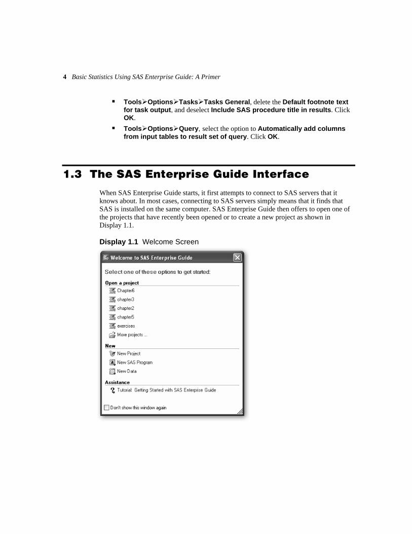
When SAS Enterprise Guide starts, it first attempts to connect to SAS servers that it knows about. In most cases, connecting to SAS servers simply means that it finds that SAS is installed on the same computer. SAS Enterprise Guide then offers to open one of the projects that have recently been opened or to create a new project as shown in Display 1.1.
Display 1.1 Welcome Screen

Chapter 1: Introduction to SAS Enterprise Guide 5
1.3.1 SAS Enterprise Guide Projects A project is the way in which SAS Enterprise Guide stores statistical analyses and their results: it records which data sets were used, what analyses were run, and what the results were. It can also record the user’s own notes on what they did and why. In the same way that a word processor loads and saves documents, so SAS Enterprise Guide does with projects. Thus, a project is a piece of statistical analysis in the same way that a document is a piece of writing. In terms of scope, a project might be the user’s approach to answering one particular question of interest. It should not be so large or diffuse that it becomes difficult to manage.
1.3.2 The User Interface The default user interface for SAS Enterprise Guide 4.1 is shown in Display 1.2.
Display 1.2 SAS Enterprise Guide User Interface
6 Basic Statistics Using SAS Enterprise Guide: A Primer
The most familiar elements of the interface are the menu bar and toolbar at the top of the window. There are four windows open and visible:
the Project Explorer window
the Project Designer window
the Task Status window
the Task List window
Moving the cursor over the task list causes the task list to scroll to the right.
For the vast majority of the examples in this book, we use only the menus and the Project Designer window. In this way the reader can safely ignore other elements of the interface, or even close them. We give a brief description of them, for completeness sake.
Toolbar and Task List offer alternative, sometimes quicker, ways to access features of SAS Enterprise Guide.
Task Status window shows what is happening while SAS Enterprise Guide is using SAS to run a program.
Project Explorer window offers an alternative view of the project to that presented in the Project Designer window. It tends to show more detail, which can be useful in some cases.
1.3.3 The Process Flow Within the Project Designer window, we can see an element labeled Process Flow, which is another concept central to SAS Enterprise Guide. Essentially, a process flow is a diagram consisting of icons that represent data sets, tasks, and outputs with arrows joining them to indicate how they relate to each other. The general term tasks includes not only statistical analyses but data manipulation.
We will begin with some examples of process flow diagrams to give an overview before describing the individual elements in more detail. An example of a Project Designer window is shown in Display 1.3.

Chapter 1: Introduction to SAS Enterprise Guide 7
Display 1.3 An Example of a Project Designer Window
The first thing to note about this example is that the Project Designer window actually contains three process flows, identified by tabs at the top of the window:
Project Process Flow (the default name)
weightgain
Post-natal Depression
To make a process flow active and bring it to the front, click on the tab. In this case, the Post-natal Depression process flow is the active one, and the title on the tab is bold to indicate that this is the case.
The first three icons in Display 1.3 represent the process of importing some data into a SAS data set. The Import Data task has as its input a raw data file, depressionIQ (depressio...), and as its output a SAS data set. The full name of the raw data file is not visible in the process flow; if the cursor is held over the icon, a window pops up with more details, including the full name, path, and location (i.e., which computer it is on). The SAS data set has been automatically given the somewhat arbitrary name SASUSER.IMPW_0007. The relationship of a task to its input and output is represented primarily by the arrows, but also by the ordering from left to right—input to the left of the task and output to the right of the task.
On the right-hand side of the process flow diagram, we can see that the SAS data set is used as input to three tasks: a Summary Tables task and two Linear Models tasks. The output from each task is an RTF (rich text format) document containing the results. RTF is one of the formats that can be chosen for output and is one particularly suited for reading into a word processor.

8 Basic Statistics Using SAS Enterprise Guide: A Primer
1.3.4 The Active Data Set Two important things to note about Display 1.3 are that the icon for the SAS data set has a dashed line around it and its label is highlighted. The dashed line indicates that the SAS data set has been selected (clicked), and this makes it the active data set. If there are multiple data sets in a project, any tasks selected from the menus will apply to the active data set. It is therefore important to be aware of which data set is active and of how to make a data set active. Each type of object and task in the process flow has its own icon, and a SAS data set can be recognized by the icon (the grid with the red ball in the bottom right corner).
A second example, shown in Display 1.4, contains four SAS data sets. The first data set results from importing some raw data from a file named LENGTHS, and the other data sets are derived from it. Generating other data sets is a common situation, where there is an original data set and one or more different versions arise from some modification of the original data. The feet data set is the active data set, so any analysis chosen from the menus would apply to that data set.
Display 1.4 A Process Flow Containing Multiple SAS Data Sets
Any of the icons in a process flow diagram can be opened by double-clicking them or right-clicking, and selecting Open. For a file, data set, or output, the contents can then be examined, printed, or copied. For a task, the settings can be examined, changed if required, and the task re-run. When a task is re-run, there is the option to replace the output from the previous run or generate new output, keeping the previous version. If the Replace option is taken, a new task icon and output icon will appear in the process flow.

Chapter 1: Introduction to SAS Enterprise Guide 9
1.4 Creating a Project
The first step in a project is adding the data. In order to be analyzed, data must be in the form of a SAS data set. Data in other formats will need to be converted or imported into a SAS data set. In many cases, the conversion or importation will have already been done.
1.4.1 Opening a SAS Data Set To add a SAS data set to a project, select File Open Data. A window like that shown in Display 1.5 will then appear, prompting a location from which to open the data. Local Computer is the user’s own computer where SAS Enterprise Guide is being used. Local Computer would also be the location for data stored on a network file server mapped to a local drive letter. For example, if the user had data stored on a network drive N: that would also count as stored on the local computer. The alternative, SAS Servers, refers to remote computers that have SAS installed and hold SAS data sets. All of the examples in this book use data stored on the local C: drive.
Display 1.5 Data Location Pop Up Window
Having selected Local Computer or a SAS Servers, browse to the location of the SAS data set, select it, and click Open. In our examples, SAS data sets are stored in the directory c:\saseg\sasdata. SAS data sets created with version 7 of SAS or a later version have the extension .sas7bdat. Data sets created by earlier versions of SAS are most likely to have the extension .sd2. The SAS data set water.sas7bdat contains measures of water hardness and mortality rates for 61 towns in England and Wales. Open that data set and the contents of the data set can then be viewed on screen as shown in Display 1.6.

10 Basic Statistics Using SAS Enterprise Guide: A Primer
Display 1.6 The Water Data Set Opened
Closing the data set, we see that a SAS data set icon, labeled water, has been added to the process flow.
1.4.2 Importing Data If the data to be analyzed are not already available as a SAS data set, they need to be imported into one, using the Import Data task. We begin with examples of importing raw data files, which are also referred to as text files or ASCII files. Such files contain only the printable characters plus spaces, tabs, and end-of-line characters. The files produced by database programs and spreadsheets are not normally in this format, although the programs usually have an export facility to create raw data files.
The data in a raw data file may be fixed width or delimited. With fixed-width data, the values for each variable are in prespecified columns. With delimited data, the data values are separated by a special character—usually a space, tab, or comma. Tab-separated files and comma-separated files are very common formats. Comma-separated data are sometimes referred to as comma-separated values and given the extension .csv. Delimited files may also contain the names of the variables, usually as the first line of the file, with the names separated by the same delimiter as the data values.
There are examples of importing both tab- and comma-delimited data, with and without the variable names, in later chapters (see the index). Here, we illustrate the use of the Import Data task with fixed-width data. The water.dat file contains a slightly different version of the data already available in the SAS data set of the same name. To import them, select File Import Data.

Chapter 1: Introduction to SAS Enterprise Guide 11
The Import Data task, as with most tasks, consists of a number of panes, each of which allows a set of options to be specified. The initial view is shown in Display 1.7.
Display 1.7 Import Data Task Opening Screen
The first pane, Region to import, is displayed. Other panes, listed in the left side of the window, are: Text Format, Column Options, and Results. In the Region to import pane, Import entire file is the default. The option to Specify line to use as column headings is for delimited files where the variable names are included in the file, usually in line 1. Hence, 1 is the default value if the option is selected. The Text Format pane allows the format to be specified as Fixed Width or Delimited and, if delimited, what delimiter is used. The default is comma-delimited. Display 1.8 shows the result of selecting Fixed Width format with this data file.

12 Basic Statistics Using SAS Enterprise Guide: A Primer
Display 1.8 Text Format Pane for Water Data
The pane shows the beginning of the file with a ruler above to indicate which columns the data values are in. Clicking on the ruler specifies where the data fields begin and end. We have put the separators at columns 2, 19, 25, and 30. The Column Options pane is shown in Display 1.9.

Chapter 1: Introduction to SAS Enterprise Guide 13
Display 1.9 Column Options Pane for Water Data
We see first that five rather than four columns have been defined. Column 5 is the blank remainder of the line after the final delimiter, so we have set the Include in output option to No. In the pane shown in Display 1.9, we can also give the variables (or columns) more meaningful names. Select Name under Column Properties and type a new name. Rename columns 1 to 4 as flag, town, Mortality, and hardness, respectively. (We deselected the option to Use column names as label for all columns to avoid having to retype these labels as well.)
We also check that other properties of the columns have been correctly assigned. In fact, Mortality and hardness have been treated as character variables when they should be numeric, but we can change the variable type using the Type option under Column Properties.
The final Results pane allows the SAS data set being created to be renamed and stored in a particular location. In this case, we leave the default settings and run the task. Display 1.10 shows the results, which are similar to the results shown previously in Display 1.6. The data set has been given an arbitrary name, SASUSER.IMPW_000A. At this point, we should scroll through the data to make sure it has all been imported correctly. Having done that, we would close the water data set as its contents are in front of the process flow. We could click on the process flow tab (labeled Project Designer)

14 Basic Statistics Using SAS Enterprise Guide: A Primer
to bring it to the front, but it keeps the workspace tidier if we close data sets and output after we have viewed them.
Display 1.10 Imported Version of Water Data
In addition to being able to import data from text files, SAS Enterprise Guide can also import data from several popular Windows programs such as Microsoft Excel and Microsoft Access. As a simple example, the file c:\saseg\data\usair.xls contains a Microsoft Excel workbook with some data on air pollution in the USA. The data are described more fully in Chapter 6 (Exercise 6.4) but need not concern us here. To import the data:
1. Select File Import Data Local Computer.
2. Browse to c:\saseg\data.
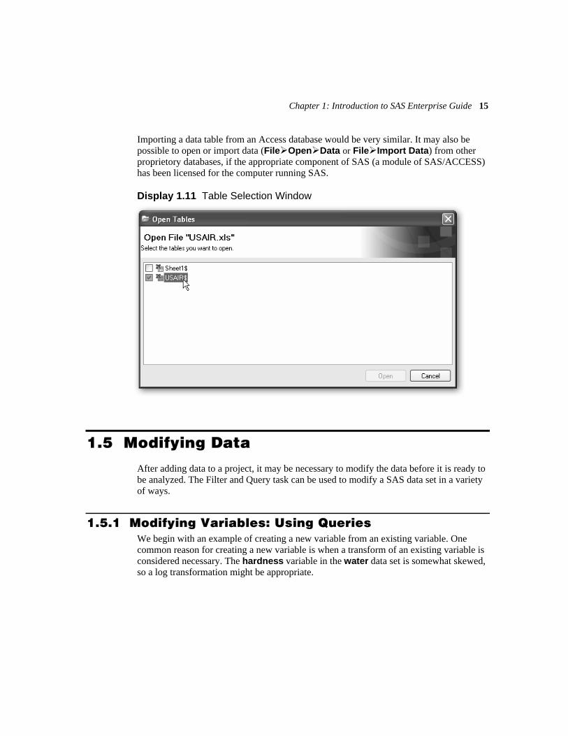
3. Select usair.xls and Open. Because the file contains more than one worksheet and only one can be imported at a time, a window like that in Display 1.11 pops up to select the worksheet to use.
4. Select USAIR and then Open. The worksheet contains the variable names in the first row. SAS Enterprise Guide has recognized this and set the options under Region to import and Column Options appropriately, so no changes are needed.
5. Run the task. It is worth noting that the ease of importing the data is due to the fact that the spreadsheet contains only the variable names and the data values. It would be simpler again if the file contained only a single worksheet.
Chapter 1: Introduction to SAS Enterprise Guide 15
Importing a data table from an Access database would be very similar. It may also be possible to open or import data (File Open Data or File Import Data) from other proprietory databases, if the appropriate component of SAS (a module of SAS/ACCESS) has been licensed for the computer running SAS.
Display 1.11 Table Selection Window
1.5 Modifying Data
After adding data to a project, it may be necessary to modify the data before it is ready to be analyzed. The Filter and Query task can be used to modify a SAS data set in a variety of ways.
1.5.1 Modifying Variables: Using Queries We begin with an example of creating a new variable from an existing variable. One common reason for creating a new variable is when a transform of an existing variable is considered necessary. The hardness variable in the water data set is somewhat skewed, so a log transformation might be appropriate.

16 Basic Statistics Using SAS Enterprise Guide: A Primer
1. Click on the water data set to make it active. There are two icons in the process flow both named water. The SAS data set that we wish to use is distinguished by its icon—the text file of the same name has a notepad icon. They can also be distinguished by holding the cursor over them, which reveals additional details of each.
2. Select the SAS data set.
3. Select Data Filter and Query. The opening screen should look like Display 1.12.
Display 1.12 Query Builder Window
The four variables in the input data set also appear in the Select Data pane because we have set the option to Automatically add columns from input tables to result set of query under Tools Options Query. Otherwise, variables from the input data set would need to be dragged across. It is worth noting in passing that the variables have icons that indicate whether they are character or numeric.

Chapter 1: Introduction to SAS Enterprise Guide 17
4. To create a new variable, select Computed Columns New Build Expression. This brings up the Advanced Expression Editor window as shown in Display 1.13.
Display 1.13 Advanced Expression Editor
The expression text specifies how the new variable is to be calculated. It can either be typed into the pane or constructed using the buttons and menus. Selecting the Functions tab shows a list of function categories with All Functions as the default. The right hand pane shows the functions by name, with a brief description of the highlighted function below.
5. Scroll down this list, click on LOG and Add to Expression. LOG(<numValue>) appears in the expression text. The <numValue> part indicates that the log function takes a numeric argument.
6. Because we want the log of the hardness variable, replace <numValue> with hardness either by simply typing hardness in or by using the Data tab. If the Data tab is used, the variable name will be prefixed with the name of the data set.
18 Basic Statistics Using SAS Enterprise Guide: A Primer
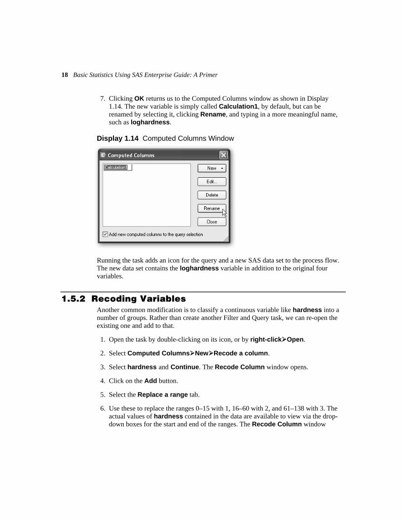
7. Clicking OK returns us to the Computed Columns window as shown in Display 1.14. The new variable is simply called Calculation1, by default, but can be renamed by selecting it, clicking Rename, and typing in a more meaningful name, such as loghardness.
Display 1.14 Computed Columns Window
Running the task adds an icon for the query and a new SAS data set to the process flow. The new data set contains the loghardness variable in addition to the original four variables.
1.5.2 Recoding Variables Another common modification is to classify a continuous variable like hardness into a number of groups. Rather than create another Filter and Query task, we can re-open the existing one and add to that.
1. Open the task by double-clicking on its icon, or by right-click Open.
2. Select Computed Columns New Recode a column.
3. Select hardness and Continue. The Recode Column window opens.
4. Click on the Add button.
5. Select the Replace a range tab.
6. Use these to replace the ranges 0–15 with 1, 16–60 with 2, and 61–138 with 3. The actual values of hardness contained in the data are available to view via the drop- down boxes for the start and end of the ranges. The Recode Column window

Chapter 1: Introduction to SAS Enterprise Guide 19
should now look like Display 1.15. Change the New column name to hardness3groups as shown.
7. Click OK, Close, and Run.
8. Reply Yes to Would you like to replace the results from the previous run? The Recode Column option within the Filter and Query task can also be used to reduce the number of categories a categorical variable has, for instance when combining categories which have too few members in. Such recoding can be done with both numeric and character variables.
Including multiple data modifications in the one Filter and Query task helps to keep the process flow diagrams simple and clear.
Display 1.15 Recode Column Window

20 Basic Statistics Using SAS Enterprise Guide: A Primer
To modify the value of a variable for some observations and not others, or to make different modifications for different groups of observations, use the Advanced Expression Editor to build a query with a conditional function. A simple example is given in Chapter 2, Section 2.3.1.
1.5.3 Splitting Data Sets: Using Filters So far we have looked at using the Filter and Query task to create and modify the values of variables and we used queries for the purpose. We now turn to the use of filters to produce subsets of the observations in a data set. We might want to form a subset of the observations in order to discard observations that have errors, or because we wish to focus our analysis on one particular group of observations. Take the water data set as an example where we want to look only at the northerly towns. Normally we would want to include the newly derived variables, and so we would use the data set calculated with the query described above.
1. Click on the water data set to make it the active data set.
2. Select Data Filter and Query.
3. Click on the Filter Data tab.
4. Location is the variable we want to filter on, so we drag and drop that into the Filter Data pane. The Edit Filter window pops up.
5. The value of location that we want to select is north. We could simply type that into the value box, but it would be safer to use the drop-down button and select Get Values.
The reason for preferring Get Values is that filters which use character variables are case sensitive: North is different from north, so if both occurred in the data set, the filter would need to include both. Using Get Values would give us the correct spelling and case as well as alerting us to any misspellings that there might be in the data set.
In our example here, the situation is straightforward and the Query Builder window should look like Display 1.16. A more complex filter can be constructed by clicking the new filter button (circled in Display 1.16) and selecting New Advanced Filter, which brings up the Advanced Expression Editor seen earlier. Another example of using filters to split the data set for separate analyses is given in Chapter 2, Section 2.2.2, and the process flow is reproduced in Display 1.4 above.

Chapter 1: Introduction to SAS Enterprise Guide 21
Display 1.16 Query Builder Window Filtering the Water Data Set
1.5.4 Concatenating and Merging Data Sets: Appends and Joins
Where two or more data sets contain the same variables (or mostly the same) but different observations, they can be combined into a single data set using Data Append Table and specifying the table(s) to be concatenated with the active data set. Concatenation is essentially the converse of the process of splitting data sets described above.
Where two data sets contain mostly the same observations but different variables, they can be combined to create a data set with all the variables using a join. Joins are yet another function of the Filter and Query task. We will illustrate a join again using the water data set. The original water data set has a variable, location, with values north and south. The version imported from the raw data has a variable, flag, where the value

22 Basic Statistics Using SAS Enterprise Guide: A Primer
‘*’ indicates the more northerly towns. To check that the two variables do in fact correspond, we will merge the data sets to produce one that has both variables.
1. Make the imported data set the active data set.
2. Select Data Filter and Query.
3. Click Add tables.
4. Select project as the location to open the data from. The list of similarly named data sets shown in Display 1.17 illustrates the potential value of giving output data sets explicit and more meaningful names. In this instance, the one simply labeled water is the one we need.
Display 1.17 List of Project Data Sets
5. Select the water data set.
6. Click OK. A Query Builder window like that shown in Display 1.18 opens.

Chapter 1: Introduction to SAS Enterprise Guide 23
Display 1.18 Query Builder Window for Join of Two Versions of the Water Data Set
All the variables from the water data set have been added and, where they had the same name, the names have been suffixed with a 1 to make them distinct.
7. Click on Join. The join is displayed, as in Display 1.19, and can be modified if necessary.

24 Basic Statistics Using SAS Enterprise Guide: A Primer
Display 1.19 Join of Two Versions of the Water Data Set
The program has recognized that both data sets contain the variable town, which uniquely identifies each observation and can therefore be used to match them. The Venn diagram in the arrow connecting them shows that an inner join will be used. Right-clicking on the Venn diagram and selecting Modify Join lists the different types of joins and explains them. A choice will need to be made if the two data sets contain different observations. Here, the two data sets contain the same observations, so the type of join makes no difference.
8. Close the Tables and Joins window.
9. Use the buttons on the right of the Select Data pane to delete Town1, Mortal, and Hardness1, and to move flag next to location.
10. Run the query.
11. Sort the resulting data set by location (Data Sort Data and Sort by location). Scrolling down the results confirms that flag and location do indeed correspond.

Chapter 1: Introduction to SAS Enterprise Guide 25
The process flow should now resemble Display 1.20. It is beginning to look a bit confusing. Several tasks and data sets have similar names (beginning with “Query”) which do not give much idea of their purpose or contents.
Display 1.20 Process Flow with Default Names
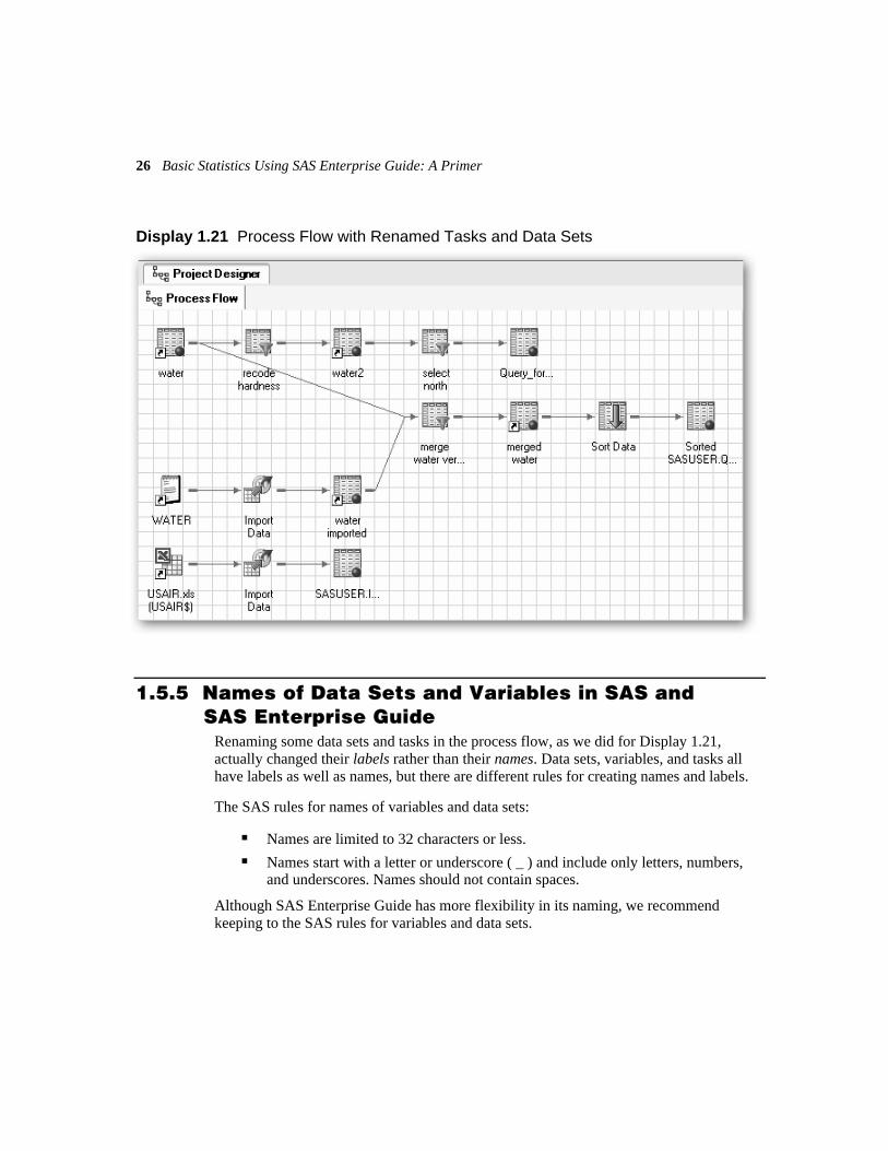
Some of the tasks and data sets could be renamed (right-click Rename) to make this clearer. Display 1.21 shows an example.
26 Basic Statistics Using SAS Enterprise Guide: A Primer
Display 1.21 Process Flow with Renamed Tasks and Data Sets
1.5.5 Names of Data Sets and Variables in SAS and SAS Enterprise Guide
Renaming some data sets and tasks in the process flow, as we did for Display 1.21, actually changed their labels rather than their names. Data sets, variables, and tasks all have labels as well as names, but there are different rules for creating names and labels.
The SAS rules for names of variables and data sets:
Names are limited to 32 characters or less.
Names start with a letter or underscore ( _ ) and include only letters, numbers, and underscores. Names should not contain spaces.
Although SAS Enterprise Guide has more flexibility in its naming, we recommend keeping to the SAS rules for variables and data sets.
Chapter 1: Introduction to SAS Enterprise Guide 27
Labels, in contrast, can contain spaces and other characters and can be up to 256 characters long. However, when there is any doubt about which is being changed, it would be safer to leave spaces out and keep to the rules for SAS names.
1.5.6 Storing SAS Data Sets: Libraries The SAS data sets created so far have been left with default names and locations. Some data set labels were altered to make the process flow easier to read. In most cases, it is not necessary to alter names and locations. When you want to control where project data sets are stored, use libraries. Essentially, a library is a folder where SAS data sets are stored. Rather than refer to the folder explicitly, the folder is assigned an alias: the library name. For example, the data sets created by the Import Data task were automatically given names like SASUSER.IMPW_xxxx. The part of the name before the period, SASUSER, is the library name and is an alias for c:\My SAS Files\9.1 on our system (it may vary depending on how SAS Enterprise Guide was set up). To store data sets in a particular folder:
1. Assign a library name for that folder using the Assign Library wizard (Tools Assign Library).
2. Type in a name, which should follow the rules for data set names but be eight characters or less; e.g., ch1.
3. Add a description if required.
4. When prompted, browse to the path of the folder; e.g., c:\saseg\libraries\ch1.
5. Continue through the wizard accepting defaults and an Assign Library icon should be added to the process flow.
This needs to be run before the library can be used in the project, so it is best to set up the libraries at the beginning of the project. Having set up the library, any data set that is given a name beginning with ch1., such as ch1.water, will be stored in the folder c:\saseg\libraries\ch1.
All SAS data sets are stored in a library. If a data set name is not prefixed with a library name, it has the implicit library name of WORK which, like SASUSER, is one of the libraries assigned automatically by SAS Enterprise Guide. However, WORK is a temporary library which means that data sets stored in it will be deleted and removed from the project when SAS Enterprise Guide is closed, although the option to move the data sets to another library is offered at that point.

28 Basic Statistics Using SAS Enterprise Guide: A Primer
1.6 Statistical Analysis Tasks
Once data in a SAS data set have been added to a project, whether directly or by importing raw data, the analysis can begin. Individual tasks are described in detail in subsequent chapters. Here, we describe some general features of the analysis tasks.
One point to bear in mind is that not all tasks that might be considered as analysis are under the Analyze menu. Several are accessed from the Describe menu, and some of the tasks under the Data menu could form part of an analysis.
A typical analysis task consists of a number of panes, each of which allows some aspect of the analysis or set of options to be specified. We begin by looking at an example taken from Chapter 5. The process flow diagram is shown in Display 1.3. Opening the first of the Linear Models tasks gives the screen shown in Display 1.22.
Display 1.22 Linear Models Task Opening Window

Chapter 1: Introduction to SAS Enterprise Guide 29
The panes are listed down the left: Task Roles, Model, Model Options, etc.
The Task Roles pane, which is selected, is where the variables that are to be used in the analysis are selected and their roles in the analysis specified. The available variables are listed in the central section, and they can be dragged from there to the specific roles in the right-hand section. The available roles vary depending on the task, but some of the most common are included here:
The Dependent variable is the response variable, the one whose values we are modeling. The numeric icon to the left indicates that only numeric variables can be assigned this role and (Limit: 1) to the right indicates that only one response variable can be included in the model. The variable ChildIQ has been assigned this role.
Quantitative variables are also numeric. The dashed line around it shows that it has been selected (clicked on) and a description of the role appears in the box below, explaining that these are continuous explanatory variables. There are no variables assigned to this role.
Classification variables are discrete explanatory variables. They can be numeric or character. If they are numeric, classification variables will tend to have relatively few distinct values. Pa_history and Mo_depression are both assigned this role.
Group analysis by variables are also discrete, numeric, or character—variables which define groups in the data. When a variable is assigned this role, the analysis is repeated for each group defined by the variable. For example, if a variable, sex, with values male and female was assigned this role, the analysis would be repeated for males and females separately. We saw earlier how to use Filter and Query to split or subset a data set. If the reason for doing this is to apply the same analysis to separate groups of observations, then using Group Analysis by with a suitable variable could be both simpler and more efficient.
Frequency count variables are used with grouped data, where each observation represents a number of individuals. The frequency count variable is the one which specifies how many individuals the observation pertains to. The most common use is in analysing tabulated data. Examples are given in Chapter 3, Sections 3.4.3 and 3.4.4.
The relative weight role is for weighted analysis.
Task panes like Model, Model Options, and Advanced Options, as their names imply, specify what model is to be fitted and how. They will be dealt with in detail in later chapters as they arise.
Many analysis tasks also produce plots of data values, predicted values, residuals, etc., each of which may be specified in the Plots pane(s).

30 Basic Statistics Using SAS Enterprise Guide: A Primer
1.7 Graphs
SAS Enterprise Guide also makes the powerful graphics facilities of SAS much easier to use. Some of these graphic facilities are available within analysis tasks and others are accessed from the Graph menu. A wide range of plots and charts are described in later chapters. Rather than describe the graph tasks here, the interested reader is referred to the index.
One point to note, however, is that the graphs produced are dependent both on the format of the results and the graph format. Both formats are specified under Tools Options Results Results General and Tools Options Results Graph. One major difference is that, when the output format is RTF, the graphs are included in the same file as the textual output and tables; when HTML output is chosen, each graph appears in a separate file with its own icon in the process flow.
1.8 Running Parts of the Process Flow
So far, we have described running individual tasks. It is also possible to run a branch of the process flow or the whole process flow. If we right-click on any task within a process flow, we will have the option to run that task or to run the branch from that task. The branch is everything to the right of the task which is directly or indirectly connected to it by the arrows. To run the whole process flow, right-click on its tab and select Run.

C h a p t e r 2
Data Description and Simple Inference
2.1 Introduction 32 2.2 Example: Guessing the Width of a Room: Analysis of Room Width
Guesses 32 2.2.1 Initial Analysis of Room Width Guesses Using Simple Summary
Statistics and Graphics 33 2.2.2 Guessing the Width of a Room: Is There Any Difference in Guesses
Made in Feet and in Meters? 40 2.2.3 Checking the Assumptions Made When Using Student’s t-Test and
Alternatives to the t-Test 47 2.3 Example: Wave Power and Mooring Methods 49
2.3.1 Initial Analysis of Wave Energy Data Using Box Plots 50 2.3.2 Wave Power and Mooring Methods: Do Two Mooring Methods Differ in
Bending Stress? 54 2.3.3 Checking the Assumptions of the Paired t-Tests 56
2.4 Exercises 57

32 Basic Statistics Using SAS Enterprise Guide: A Primer
2.1 Introduction
In this chapter, we will describe how to get informative numerical summaries of data and graphs which allow us to assess various properties of the data. In addition, we will show how to test whether different populations have the same mean value. The statistical topics covered are:
Summary statistics such as means and variances
Graphs such as histograms and box-plots
Student’s t-test
2.2 Example: Guessing the Width of a Room: Analysis of Room Width Guesses
Shortly after metric units of length were officially introduced in Australia in the 1970s, each one of 44 students was asked to guess, to the nearest meter, the width of the lecture hall in which they were sitting. Another group of 69 students in the same room was asked to guess the width in feet, to the nearest foot. The measured width of the room was 13.1 meters (43.0 feet). The data, collected by Professor T. Lewis, are given here in Table 2.1, which is taken from Hand et al. (1994). Of primary interest here is whether the guesses made in meters differ from the guesses made in feet, and which set of guesses give the most accurate assessment of the “true” width of the room (accuracy in this context implies guesses which are closer to the measured width of the room).
Table 2.1 Room Width Estimates
Guesses in meters
8 9 10 10 10 10 10 10 11 11 11 11 12 12 13 13 13 14 14 14 15 15 15 15 15 15 15 15 16 16 16 17 17 17 17 18 18 20 22 25 27 35 38 40
Guesses in feet
24 25 27 30 30 30 30 30 30 32 32 33 34 34 34 35 35 36 36 36 37 37 40 40 40 40 40 40 40 40 40 41 41 42 42 42 42 43 43 44 44 44 45 45 45 45 45 45 46 46 47 48 48 50 50 50 51 54 54 54 55 55 60 60 63 70 75 80 94

Chapter 2: Data Description and Simple Inference 33
2.2.1 Initial Analysis of Room Width Guesses Using Simple Summary Statistics and Graphics
How should we begin our investigation of the room-width guesses data that are given in Table 2.1? As with most data sets, the initial data analysis steps should involve the calculation of simple summary statistics, such as means and variances, and graphs and diagrams that convey clearly the general characteristics of the data, and perhaps enable any unusual observations or patterns in the data to be detected. Such summary statistics and graphs are very easy to obtain using SAS Enterprise Guide. First, we will show how to read in the data, convert the room widths in meters into feet by multiplying them by 3.28, and then calculate the means and standard deviations of the meter estimates and the feet estimates.
The data are stored in a tab-separated file, lengths.tab. To read them in:
1. Select File Import Data.
2. Select Local Computer as the source.
3. Browse to the folder that contains the file, c:\saseg\data, select lengths.tab, and Open. The Import Data window opens.
4. Select Text Format, and click the Delimited and Tab buttons.
5. Select Column Options. SAS Enterprise Guide has recognized that the file contains two columns of data, the first character and the second numeric.
6. Uncheck the box Use column name as label for all columns.
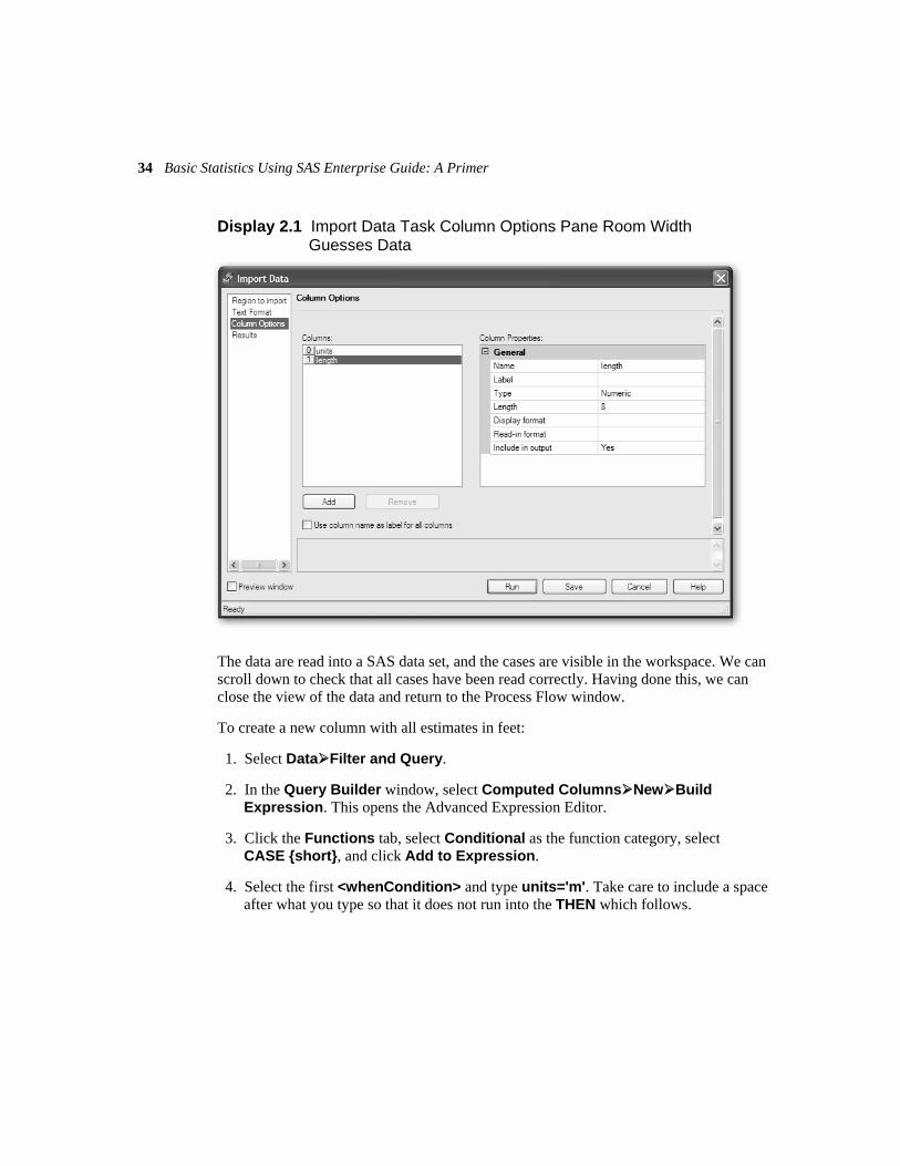
7. Rename the columns to units and length. The window should now look like Display 2.1.
8. Under Results, click Browse, and rename the output file to SASlengths.
9. Run the procedure.
34 Basic Statistics Using SAS Enterprise Guide: A Primer
Display 2.1 Import Data Task Column Options Pane Room Width Guesses Data
The data are read into a SAS data set, and the cases are visible in the workspace. We can scroll down to check that all cases have been read correctly. Having done this, we can close the view of the data and return to the Process Flow window.
To create a new column with all estimates in feet:
1. Select Data Filter and Query.
2. In the Query Builder window, select Computed Columns New Build Expression. This opens the Advanced Expression Editor.
3. Click the Functions tab, select Conditional as the function category, select CASE {short}, and click Add to Expression.
4. Select the first <whenCondition> and type units='m'. Take care to include a space after what you type so that it does not run into the THEN which follows.

Chapter 2: Data Description and Simple Inference 35
5. In the same way, replace the first <resultExpression> with length*3.28, the second <whenCondition> with units='f' and the second <resultExpression> with length, and click OK. In each instance, take care to insert a space after what you type.
6. The entire expression should now read CASE WHEN units='m' THEN length*3.28 WHEN units='f' THEN length END as shown in Display 2.2. Click OK. In the pop-up window, rename Calculation1 to feet, and then Close.
Display 2.2 Advanced Expression Editor
It helps to keep the process flow clear if both the query and the output file are given meaningful names. For example, name the query Meters2Feet and the output data set SASlengths2. The results appear in the workspace and again we scroll through them to check that they are correct and close the data set.
Deriving Summary Statistics Summary statistics could be produced with the task of that name (Describe Summary Statistics) but Distribution Analysis is more flexible and produces the graphs that we will use as well as summary statistics.

36 Basic Statistics Using SAS Enterprise Guide: A Primer
1. Select Describe Distribution Analysis.
2. Under Task Roles, the Analysis variable is feet. To compare the summaries for each set of guesses, treat the units variable as a Classification variable. This generates separate results for each value of units.
3. Under Tables, select only Basic measures for now.
The results are shown in Table 2.2.
Table 2.2 Summary Statistics for Room Width Guesses Data
(a) Guesses made in feet
Basic Statistical Measures
Location Variability
Mean 43.69565 Std Deviation 12.49742
Median 42.00000 Variance 156.18542
Mode 40.00000 Range 70.00000
Interquartile Range 12.00000
(b) Guesses made in meters and then converted to feet
Basic Statistical Measures
Location Variability
Mean 52.55455 Std Deviation 23.43444
Median 49.20000 Variance 549.17310
Mode 49.20000 Range 104.96000
Interquartile Range 19.68000
What do the summary statistics tell us about the two sets of guesses? It appears that the guesses made in feet are closer to the measured room width and less variable than the guesses made in meters suggesting that the guesses made in the more familiar units, feet, are more accurate than those made in the recently introduced units, meters. But often such apparent differences in means and in variation can be traced to the effect of one or two unusual observations that statisticians like to call outliers. Such observations can usually be uncovered by some simple graphics, and here we shall construct box plots of the two sets of guesses after converting the guesses made in meters to feet.

Chapter 2: Data Description and Simple Inference 37
Constructing Box Plots A box plot is a graphical display useful for highlighting important distributional features of a continuous measurement. The diagram is based on what is known as the five-number summary of a data set, the numbers in question being the minimum, the lower quartile, the median, the upper quartile, and the maximum. The box plot is constructed by first drawing a box with ends at the lower and upper quartiles of the data. Next, a horizontal line (or some other feature) is used to indicate the position of the median within the box, and then lines are drawn from each end of the box to points defined by the upper quartile plus 1.5 times the interquartile range (the difference between the upper and lower quartiles) and the lower quartile minus 1.5 times the interquartile range. Any observations outside these limits are represented individually by some means in the finished graphic. Such observations are likely candidates to be labeled outliers. The resulting diagram schematically represents the body of the data minus the extreme observations and is particularly useful for comparing the distributional features of a measurement made in different groups.
Distribution analysis also produces box plots, so we can rerun that task to get the plots.
1. In the Process Flow window, reopen the task (double-click its icon or right-click Open).
2. In Plots, select Box plot.
3. Click Run.
4. Reply Yes to Would you like to replace the results from the previous run?
The resulting plots are shown in Figure 2.1; they indicate that both sets of guesses contain a number of possible outliers and also that the guesses made in meters are skewed (have a longer tail) and are more variable than the guesses made in feet. We shall return to these findings in the next subsection.

38 Basic Statistics Using SAS Enterprise Guide: A Primer
Figure 2.1 Box Plots of Room Width Guesses Made in Feet and in Meters (after Conversion to Feet)
Constructing Histograms and Stem-and-Leaf Plots The box plot is our favorite graphic for comparing the distributional properties of a measurement made in different groups, but there are other graphics available within distribution analysis: histograms and stem-and-leaf plots. In a histogram, class frequencies are represented by the areas of rectangles centered on the class interval; if class intervals are all equal, then the heights of the rectangles are proportional to the observed frequencies. A stem-and-leaf plot has the shape of the corresponding histogram; but, by also retaining the actual observation values, gives more information. Again, we can rerun the procedure to include these. Stem-and-leaf plots are included in text based plots.
The resulting plots are all shown in Figure 2.2; they all show clearly the greater skewness in the guesses made in meters.

Chapter 2: Data Description and Simple Inference 39
Figure 2.2 Histograms and Stem and Leaf Plots for Room Width Guesses Data
Stem Leaf # Boxplot 9 4 1 * 8 8 0 1 0 7 5 1 0 7 0 1 0 6 6 003 3 | 5 55 2 | 5 0001444 7 | 4 55555566788 11 +-----+ 4 00000000011222233444 20 *--+--* 3 5566677 7 +-----+ 3 000000223444 12 | 2 57 2 | 2 4 1 | ----+----+----+----+ Multiply Stem.Leaf by 10**+1
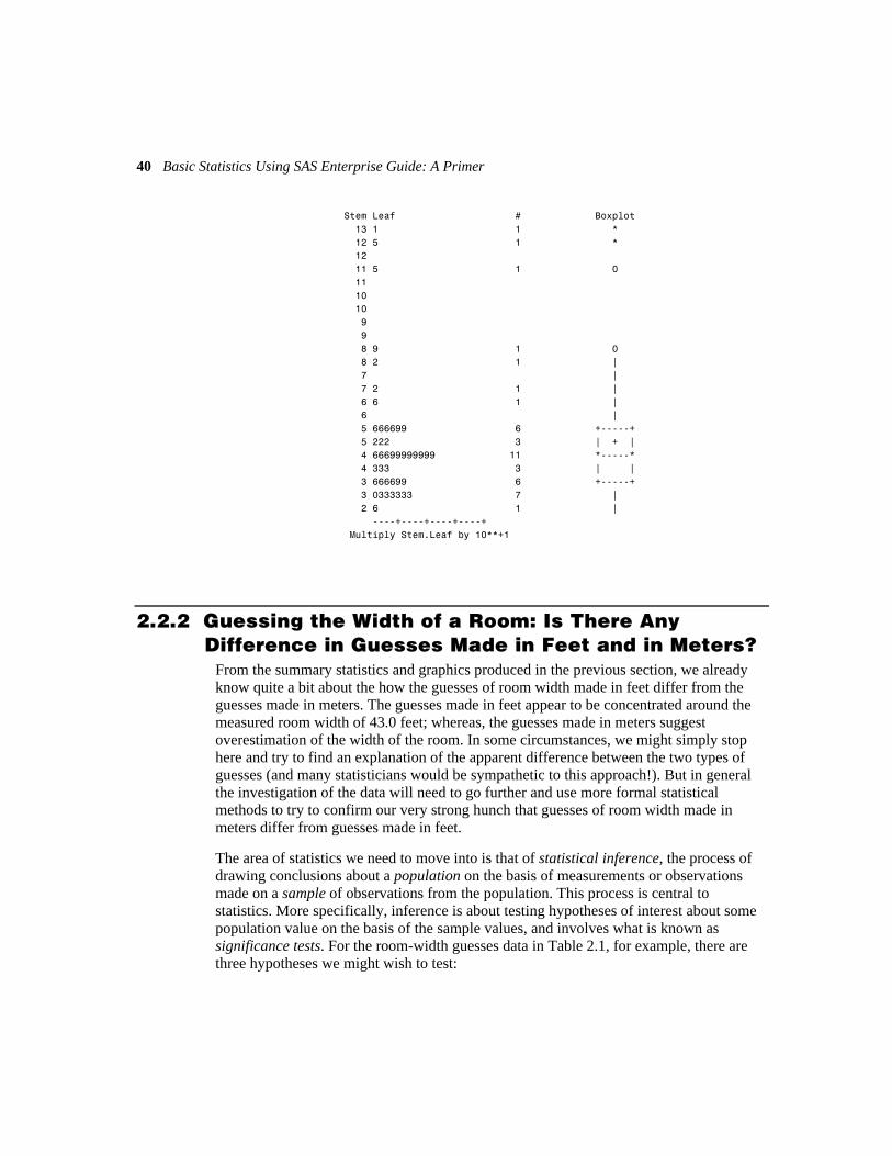
40 Basic Statistics Using SAS Enterprise Guide: A Primer
Stem Leaf # Boxplot 13 1 1 * 12 5 1 * 12 11 5 1 0 11 10 10 9 9 8 9 1 0 8 2 1 | 7 | 7 2 1 | 6 6 1 | 6 | 5 666699 6 +-----+ 5 222 3 | + | 4 66699999999 11 *-----* 4 333 3 | | 3 666699 6 +-----+ 3 0333333 7 | 2 6 1 | ----+----+----+----+ Multiply Stem.Leaf by 10**+1
2.2.2 Guessing the Width of a Room: Is There Any Difference in Guesses Made in Feet and in Meters?
From the summary statistics and graphics produced in the previous section, we already know quite a bit about the how the guesses of room width made in feet differ from the guesses made in meters. The guesses made in feet appear to be concentrated around the measured room width of 43.0 feet; whereas, the guesses made in meters suggest overestimation of the width of the room. In some circumstances, we might simply stop here and try to find an explanation of the apparent difference between the two types of guesses (and many statisticians would be sympathetic to this approach!). But in general the investigation of the data will need to go further and use more formal statistical methods to try to confirm our very strong hunch that guesses of room width made in meters differ from guesses made in feet.
The area of statistics we need to move into is that of statistical inference, the process of drawing conclusions about a population on the basis of measurements or observations made on a sample of observations from the population. This process is central to statistics. More specifically, inference is about testing hypotheses of interest about some population value on the basis of the sample values, and involves what is known as significance tests. For the room-width guesses data in Table 2.1, for example, there are three hypotheses we might wish to test:

Chapter 2: Data Description and Simple Inference 41
In the population of guesses made in meters, the mean is the same as the true room width, namely 13.1 meters. Formally we might write this hypothesis as
0H : 13.1mμ =
where 0H stands for null hypothesis.
In the population of guesses made in feet, the mean is the same as the true room width namely 43.0 feet; i.e.,
0H : 43.0fμ =
After the conversion of meters into feet, the population means of both types of guess are equal or in formal terms
0H : x3.28m fμ μ=
It might be imagined that a conclusion about the last of these three hypotheses would be implied from the results found for the first two but, as we shall see later, this is not the case.
Applying Student’s t-Test to the Guesses of Room Width Testing hypotheses about population means requires what is know as Student’s t-test. The test is described in detail in Altman (1991), but in essence involves the calculation of a test statistic from sample means and standard deviations, the distribution of which is known if the null hypothesis is true and certain assumptions are met. From the known distribution of the test statistic, a p-value can be found.
The p-value is probably the most ubiquitous statistical index found in the applied sciences literature and is particularly widely used in biomedical and psychological research. So, just what is the p-value? Well, the p-value is the probability of obtaining the observed data (or data that represent a more extreme departure from the null hypothesis) if the null hypothesis is true, and was first proposed as part of a quasi-formal method of inference by a famous statistician, Ronald Aylmer Fisher, in his influential 1925 book, Statistical Methods for Research Workers. For Fisher, the p-value represented an attempt to provide a relatively informal measure of evidence against the null hypothesis; the smaller the p-value, the greater the evidence that the null hypothesis is incorrect.
But sadly, Fisher’s informal approach to interpreting the p-value was long ago abandoned in favor of a simple division of results into significant and nonsignificant on the basis of comparing the p-value with some largely arbitrary threshold value such as 0.05. The implication of this division is that there can always be a simple “yes” (significant) or “no” (nonsignificant) answer as the fundamental result from a study. This is clearly false.

42 Basic Statistics Using SAS Enterprise Guide: A Primer
Used in this way, hypothesis testing is of limited value. In fact, overemphasis on hypothesis testing and the use of p-values to dichotomize significant or nonsignificant results has distracted from other more useful approaches to interpreting study results, in particular the use of confidence intervals. Such intervals are far more useful alternatives to p-values for presenting results in relation to a statistical null hypothesis and give a range of values for a quantity of interest that includes the population value of the quantity with some specified probability. Confidence intervals are described in detail in Altman (1991). In essence, the significance test and associated p-value relate to what the population quantity of interest is not; the confidence interval gives a plausible range for what the quantity is.
So, after this rather lengthy digression, let’s apply the relevant Student’s t-tests to the three hypotheses we are interested in assessing on the room-width data. The first two hypotheses require the application of the single sample t-test separately to each set of guesses.
We begin by returning to the Process Flow window with the lengths data by clicking on its tab. To analyze the two sets of guesses separately, we will split the data into two subsets:
1. Click on SASwaves2 to make it the active data set.
2. Select Data Filter and Query, click the Filter Data tab, and drag units across.
3. In the Edit Filter window, type m in the value box. Click OK. This returns you to the Query Builder window (see Display 2.3). Change the output name to meters and click Run.
4. Repeat this by typing f in the value box and naming the output feet.

Chapter 2: Data Description and Simple Inference 43
Display 2.3 Filter Data Selecting Guesses Made in Meters
The t Test procedure can be used to apply the one sample t-test to each set of guesses:
1. Select the meters data set.
2. Select Analyze ANOVA t Test.
3. Under t Test type, select One Sample.
4. Under Task Roles, choose length as the analysis variable (not feet because we want the original units).
5. Under Analysis, enter 13.1 for Specify the test value for the null hypothesis (Display 2.4).
6. Under Titles, amend the title to include H0=13.1.
7. Click Run.
For the other set of guesses, select the feet data set and repeat entering 43 as the test value. Change the title to include H0=43 and click Run.

44 Basic Statistics Using SAS Enterprise Guide: A Primer
Display 2.4 Single Sample t-Test: Specifying the Value of the Null Hypothesis
The results are shown in Table 2.3. Let’s now look at these results in some detail. Looking first at the two p-values, we see that there is no evidence that the guesses made in feet differ in mean from the true width of the room, 43 feet; the 95 % confidence interval here is [40.69,46.70], which includes the true width of the room. But there is considerable evidence that the guesses made in meters do differ from the true value of 13.1 meters; here, the confidence interval is [13.85,18.20], and the students appear to systematically overestimate the width of the room when guessing in meters.

Chapter 2: Data Description and Simple Inference 45
Table 2.3 Results of Single Sample t-Tests for Room-Width Guesses Made in Meters and for Guesses Made in Feet (a) Guesses in meters
Statistics
Variable N
Lower
CL
Mean Mean
Upper
CL
Mean
Lower
CL
Std Dev Std Dev
Upper
CL
Std Dev Std Err Min Max
Length 44 13.851 16.023 18.195 5.9031 7.1446 9.0525 1.0771 8 40
T-Tests
Variable DF T Value Pr > |t|
Length 43 2.71 0.0095
(b) Guesses in feet
Statistics
Variable N
Lower
CL
Mean Mean
Upper
CL
Mean
Lower
CL
Std Dev Std Dev
Upper
CL
Std Dev Std Err Min Max
length 69 40.693 43.696 46.698 10.704 12.497 15.018 1.5045 24 94
T-Tests
Variable DF T Value Pr > |t|
Length 68 0.46 0.6453
Now, it might be thought that our third hypothesis discussed above, namely that the mean of the guesses made in feet and the mean of the guesses made in meters (after conversion to feet) are the same, can be assessed simply from the results given in Table 2.3. Since the population mean of guesses made in feet apparently does not differ from the true width of the lecture room, but the population mean of guesses made in meters does differ from the true width, can we not simply infer that the population means of the two types of guesses differ from each other? Not necessarily; to assess the equality of means hypothesis correctly, we need to apply an independent samples t-test to the data. We again use the t-test task.

46 Basic Statistics Using SAS Enterprise Guide: A Primer
1. Select the SASlengths2 data set (click on its icon).
2. Select Analyze ANOVA t Test.
3. Under t Test type, select Two Sample.
4. Under Task Roles, assign feet as the Analysis variable and units as the Group by variable (not the Group analysis by variable).
5. Click Run.
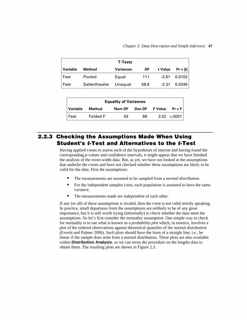
The results of applying this test are shown in Table 2.4. Looking first at the p-value when equality of variances is assumed (p=0.0102), we see that there is considerable evidence that the population means of the two types of guesses do indeed differ. The confidence interval for the difference, [–15.57,–2.15], indicates that the guesses made in feet have a mean that is between 16 and 2 feet lower than the guesses made in meters.
Table 2.4 Results of Applying Independent Samples t-Test to the Room-Width Guesses Data
Statistics
Variable Units N
Lower
CL
Mean Mean
Upper
CL
Mean
Lower
CL
Std Dev Std Dev
Upper
CL
Std Dev Std Err Min
Feet F 69 40.693 43.696 46.698 10.704 12.497 15.018 1.5045 24
Feet M 44 45.43 52.555 59.679 19.362 23.434 29.692 3.5329 26.24
Feet Diff (1-2) -15.57 -8.859 -2.145 15.524 17.562 20.22 3.3881
Statistics
Variable Units Maximum
Feet F 94
Feet M 131.2
Feet Diff (1-2)
Chapter 2: Data Description and Simple Inference 47
T-Tests
Variable Method Variances DF t Value Pr > |t|
Feet Pooled Equal 111 -2.61 0.0102
Feet Satterthwaite Unequal 58.8 -2.31 0.0246
Equality of Variances
Variable Method Num DF Den DF F Value Pr > F
Feet Folded F 43 68 3.52 <.0001
2.2.3 Checking the Assumptions Made When Using Student’s t-Test and Alternatives to the t-Test
Having applied t-tests to assess each of the hypotheses of interest and having found the corresponding p-values and confidence intervals, it might appear that we have finished the analysis of the room-width data. But, as yet, we have not looked at the assumptions that underlie the t-tests and have not checked whether these assumptions are likely to be valid for the data. First the assumptions:
The measurements are assumed to be sampled from a normal distribution.
For the independent samples t-test, each population is assumed to have the same variance.
The measurements made are independent of each other.
If any (or all) of these assumptions is invalid, then the t-test is not valid strictly speaking. In practice, small departures from the assumptions are unlikely to be of any great importance, but it is still worth trying (informally) to check whether the data meet the assumptions. So let’s first consider the normality assumption. One simple way to check for normality is to use what is known as a probability plot which, in essence, involves a plot of the ordered observations against theoretical quantiles of the normal distribution (Everitt and Palmer 2006). Such plots should have the form of a straight line; i.e., be linear if the sample does arise from a normal distribution. These plots are also available within Distribution Analysis, so we can rerun the procedure on the lengths data to obtain them. The resulting plots are shown in Figure 2.3.

48 Basic Statistics Using SAS Enterprise Guide: A Primer
Figure 2.3 Probability Plots for the Room Width Guesses Made in Feet and in Meters
20406080
100120140
feet
f
1 5 10 25 50 75 90 95 99
20406080
100120140
feet
m
Normal Percentiles
Both plots, but particularly the plot for the guesses in meters, depart from linearity, throwing the normality assumption required for the t-test to be valid into some doubt. This possible non-normality—combined with the evidence that two types of guesses have different variances obtained from both the initial examination of the data and the test for equality of variances (Altman 1991) given in Table 2.4—suggests that some caution is needed in interpreting the results from our t-tests. Fortunately, the t-test is known to be relatively robust against departures both from normality and the homogeneity assumption, although it is somewhat difficult to predict how a combination of non-normality, heterogeneity, and outliers will affect the test.
Since the test for equality of variance given in Table 2.4 has an associated p-value <0.001, we should perhaps first consider using a modified version of the t-test in which the equality of variance assumption is dropped (Altman 1991). The p-value of the modified test (Satterthwaite test) is also given in Table 2.4 and, although less significant than the usual form of the t-test, still shows evidence for a difference in the population means of the two types of room-width guesses.

Chapter 2: Data Description and Simple Inference 49
Here however, given the existence of outliers in the data and their possible non-normality, we might ask whether an alternative test is available that is both insensitive to the effect of outliers and does not assume normality.
Wilcoxon-Mann-Whitney Test An alternative to Student’s t-test, which does not depend on the assumption of normality, is the Wilcoxon-Mann-Whitney test; this test, since it is based on the ranks of the observations, is also unlikely to be affected greatly by outliers. The Wilcoxon-Mann-Whitney test, which is described in detail in Altman (1991), assesses whether the distribution of the measurements in the two groups are the same. We can apply the test here as follows:
1. Select Analyze ANOVA Nonparametric One-Way Anova.
2. Under Task Roles assign feet the role of Dependent variable, and assign units that of Independent variable.
3. Under Analysis, select only Wilcoxon, and uncheck the other options.
4. Click Run.
The p-value for the test is 0.028 confirming the difference in location between the guesses in feet and the guesses in meters.
2.3 Example: Wave Power and Mooring Methods
In a design study for a device to generate electricity from wave power at sea, experiments were carried out on scale models in a wave tank to establish how the choice of mooring method for the system affected the bending stress produced in part of the device. The wave tank could simulate a wide range of sea states (rough, calm, moderate, etc.) and the model system was subjected to the same sample of sea states with each of two mooring methods, one of which was considerably cheaper than the other. The resulting data giving root mean square bending moment in Newton meters are shown in Table 2.5. These data are taken from Hand et al. (1994). The question of interest is whether bending stress differs for the two mooring methods.

50 Basic Statistics Using SAS Enterprise Guide: A Primer
Table 2.5 Wave Energy Device Mooring Data
Sea State Method I Method II
1 2.23 1.82
2 2.55 2.42
3 7.99 8.26
4 4.09 3.46
5 9.62 9.77
6 1.59 1.40
7 8.98 8.88
8 0.82 0.87
9 10.83 11.20
10 1.54 1.33
11 10.75 10.32
12 5.79 5.87
13 5.91 6.44
14 5.79 5.87
15 5.50 5.30
16 9.96 9.82
17 1.92 1.69
18 7.38 7.41
2.3.1 Initial Analysis of Wave Energy Data Using Box Plots
For the wave energy data in Table 2.5, we will construct box plots of the bending stresses for each mooring method and, for reasons which will become apparent in the next subsection, it is also useful to have a look at the box plot of the differences between the pairs of observations made for the same sea state.
To keep the analyses of the two examples separate, we open a new Process Flow window for the waves data.

Chapter 2: Data Description and Simple Inference 51
1. Select File New Process Flow.
2. Rename this new process flow Waves (right-click on the tab and select Rename). We could also rename the other process flow Lengths at this point.
The data are stored in a tab-separated file, waves.tab. To read them in:
1. Select File Import Data.
2. Select Local Computer as the source.
3. Then browse to the folder that contains the file, c:\saseg\data, select waves.tab, and click Open. The Import Data window opens.
4. Under Text Format, click the Delimited and Tab buttons.
5. Under Column Options, SAS Enterprise Guide has recognized that the file contains three columns of numeric data. We rename these to pairno, rsmb1, and rmsb2.
6. Under Results, change the name of the output data set to SASwaves.
7. Click Run.
The data are read into a SAS data set and are shown in the workspace.
To create a new variable with the differences:
1. Select Data Filter and Query.
2. In the Query Builder window, select Computed Columns New Build Expression.
3. In the Advanced Expression Editor in the Expression text window, type rsmb1 – rsmb2, and click OK.
4. In the Computed window, rename Calculation1 to difference, and then Close.
5. Name the query calc_difference and the output data set SASwaves2.
6. Run the query.
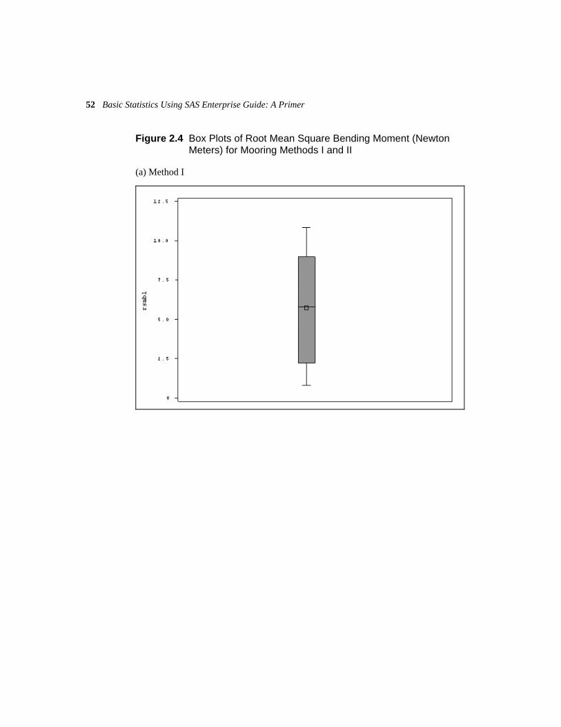
Distribution Analysis (Describe Distribution Analysis) is used to produce box plots for rmsb1, rmsb2 (see Figure 2.4), and difference (see Figure 2.5). All three are assigned the roles of Analysis variables.
52 Basic Statistics Using SAS Enterprise Guide: A Primer
Figure 2.4 Box Plots of Root Mean Square Bending Moment (Newton Meters) for Mooring Methods I and II
(a) Method I

Chapter 2: Data Description and Simple Inference 53
(b) Method II

54 Basic Statistics Using SAS Enterprise Guide: A Primer
Figure 2.5 Box Plot of Differences of Root Mean Square Bending Moment for the Two Mooring Methods
The box plot of differences in Figure 2.5 suggests that there may be one outlying observation that we may wish to check, and a small degree of skewness—although with only 18 observations, drawing any conclusions about the distributional properties of the data is difficult.
2.3.2 Wave Power and Mooring Methods: Do Two Mooring Methods Differ in Bending Stress?
Now, we can move on to consider more formally the questions of interest about the wave energy data. Superficially, these data look to be of a very similar format to the room-width guesses data, but closer consideration shows that there is a fundamental difference in that the observations are paired; i.e., the bending stress for each of the two mooring methods is, in each case, based on the same sea state. Consequently, these observations are more likely to be correlated rather than independent. To test whether there is a difference in the mean bending stress of the two methods of mooring, we use what is called a paired t-test (Altman 1991); essentially, this test is the same as the single sample

Chapter 2: Data Description and Simple Inference 55
t-test used previously for the room width data but here the null hypothesis is that the population mean of the differences of the paired observations is zero. To apply the test:
1. Select the SASwaves2 data set.
2. Select Analyze ANOVA t Test.
3. Under t Test type, choose Paired.
4. Under Task Roles, assign rsmb1 and rmsb2 as the Paired variables (Display 2.5).
5. Run the procedure.
Display 2.5 Task Roles Pane for Matched Pairs t-Test
The results are shown in Table 2.6. The p-value for the test is 0.38, and the 95% confidence interval for the mean of the differences is [–0.083, 0.206]. There is no evidence of any difference in the mean bending stress of the two mooring methods.

56 Basic Statistics Using SAS Enterprise Guide: A Primer
Table 2.6 Paired t-Test for Wave Energy Mooring Data
Statistics
Difference N
Lower
CL
Mean Mean
Upper
CL
Mean
Lower
CL
Std Dev Std Dev
Upper
CL
Std Dev Std Err Min
rmsb1 - rmsb2 18 -0.083 0.0617 0.2059 0.2177 0.2901 0.4349 0.0684 0.53
Statistics
Difference Maximum
rmsb1 - rmsb2 0.63
T-Tests
Difference DF T Value Pr > |t|
rmsb1 - rmsb2 17 0.90 0.3797
2.3.3 Checking the Assumptions of the Paired t-Tests For the paired t-test to be valid, the differences between the paired observations need to be normally distributed. We could use a probability plot to assess the required normality of the differences but, with only 18 observations for the wave data, the plot would not be very useful. Since we cannot satisfactorily assess the normality assumption for these data, we might wish to consider a nonparametric alternative; this would be the Wilcoxon signed rank test.
Wilcoxon Signed Rank Test The non-parametric analogue of the paired t-test is Wilcoxon’s signed rank test (Altman 1991). As with the Wilcoxon-Mann-Whitney test described above, the signed rank test uses only the ranks of the observations and does not assume normality for the observations; the test can be applied within Distribution Analysis.
1. Select Analyze Distribution Analysis.
2. Under Task Roles, assign difference as the Analysis variable.
3. Under Tables, select Tests for location.

Chapter 2: Data Description and Simple Inference 57
This is also an alternative way of applying a matched pairs t-test, as can be seen from the results in Table 2.7.
Table 2.7 Wilcoxon Signed Rank Test for Wave Energy Mooring Data
Tests for Location: Mu0=0
Test Statistic p Value
Student's t T 0.901934
Pr > |t| 0.3797
Sign M 1 Pr >= |M| 0.8145
Signed Rank S 23.5 Pr >= |S| 0.3194
The test gives a p-value of 0.319 confirming the result from the paired t-test.
2.4 Exercises
Exercise 2.1 The babies data set gives the recorded birthweights of 50 infants who displayed severe idiopathic respiratory distress syndrome (SIRDS). SIRDS is a serious condition that can result in death and did so in the case of 27 of these children. One of the questions of interest about these data is whether the babies who died differed in birthweight from the babies who survived. Use some suitable graphical techniques to carry out an initial analysis of these data and then find a 95% confidence interval for the difference in mean birthweight for SIRDS babies who die and SIRDS babies who live.
Birthweights (kg)
Survived
1.130 1.575 1.680 1.760 1.930 2.015 2.090 2.600
2.700 2.950 3.160 3.400 3.640 2.830 1.410 1.715
1.720 2.040 2.200 2.400 2.550 2.570 3.005
Died
1.050 1.175 1.230 1.310 1.500 1.600 1.720 1.750
1.770 2.275 2.500 1.030 1.100 1.185 1.225 1.262
1.295 1.300 1.550 1.820 1.890 1.940 2.200 2.270
2.440 2.560 2.370

58 Basic Statistics Using SAS Enterprise Guide: A Primer
Exercise 2.2 The data in the choles data set were collected by the Western Collaborative Group Study carried out in California in 1960–1961. In this study, 3,154 middle-aged men were used to investigate the possible relationship between behavior pattern and the risk of coronary heart disease. The data set contains data from the 38 heaviest men in the study (all weighing at least 225 pounds). Cholesterol measurements (mg per 100ml) and behavior type were recorded; type A behavior is characterized by urgency, aggression, and ambition; type B behavior is relaxed, non-competitive, and less hurried. The question of interest is whether, in heavy middle-aged men, cholesterol level is related to behavior type. Investigate the question of interest in any way you feel is appropriate, paying particular attention to assumptions and to any observations that might possibly distort conclusions.
Type A:
233 291 312 250 246 197 268 224 329 239 254 276 234 181 248 252 202 218 325
Type B:
420 185 263 246 224 212 188 250 148 169 226 175 242 153 183 137 202 194 213
Exercise 2.3 The data in diet come from a study of the Stillman diet, a diet that consists primarily of protein and animal fats, and restricts carbohydrate intake. In diet, triglyceride values (mg/100ml) are given for 16 participants both before beginning the diet and at the end of a period of time following the diet. Here, interest is on whether there has been a change in triglyceride level that might be attributed to the diet. Carry out an appropriate hypothesis test to investigate whether there has been a change in triglyceride level using any graphics that you think might be helpful in interpreting the test.

Chapter 2: Data Description and Simple Inference 59
Subject Baseline Final
1 159 1942 93 1223 130 158
4 174 1545 148 93
6 148 907 85 101
8 180 999 92 183
10 89 8211 204 100
12 182 10413 110 72
14 88 10815 134 110
16 84 81

60 Basic Statistics Using SAS Enterprise Guide: A Primer

C h a p t e r 3
Dealing with Categorical Data
3.1 Introduction 62 3.2 Example: Horse Race Winners 62
3.2.1 Looking at Horse Race Winners Using Some Simple Graphics:
Bar Charts and Pie Charts 62 3.2.2 Horse Race Winners: Does Starting Stall Position Predict Horse Race
Winners? 66 3.3 Example: Brain Tumors 68
3.3.1 Tabulating the Brain Tumor Data into a Contingency Table 69 3.3.2 Do Different Types of Brain Tumors Occur More Frequently at Particular
Sites? The Chi-Square Test 70 3.4 Example: Suicides and Baiting Behavior 71
3.4.1 How Is Baiting Behavior at Suicides Affected by Season?
Fisher’s Exact Test 72 3.5 Example: Juvenile Felons 75
3.5.1 Juvenile Felons: Where Should They Be Tried? McNemar’s Test 75
3.6 Exercises 75

62 Basic Statistics Using SAS Enterprise Guide: A Primer
3.1 Introduction
In this chapter, we discuss how to deal with various aspects of the analysis of data containing categorical variables; that is, variables that classify the observations in some way. Some examples of categorical variables are gender, marital status, and social class. Numbers might be used as convenient labels for the categories of categorical variables but have no numerical significance. When using categorical variables, we can simply count the number of our sample—or how many—that fall into each category of a variable, or into a combination of the categories of two or more categorical variables. In this chapter, the statistical topics to be covered are:
Graphical summary of one-way tables, bar charts, and pie charts
Testing for association of two categorical variables—Chi-square tests for independence
Testing for association of two categorical variables when some observed counts are small—Fisher’s exact test
Testing for equal probability of an event in matched pairs data—McNemar’s test
3.2 Example: Horse Race Winners
The data shown in Table 3.1 show the starting stalls of the winners in 144 horse races held in the U.S. All 144 races took place on a circular track and all races relate to races with eight horses each. Starting stall 1 is closest to the rail on the inside of the track. Interest here lies in assessing how the chances of a horse winning a race are affected by its position in the starting lineup.
Table 3.1 Horse Racing Data after Classification
Starting stall 1 2 3 4 5 6 7 8 Number of winners 29 19 18 25 17 10 15 11
3.2.1 Looking at Horse Race Winners Using Some Simple Graphics: Bar Charts and Pie Charts
The horse racing data are in a SAS data set, racestalls, which contains a single variable giving the stall number for each of the 144 winners. To add the data set to the project:
1. Select File Open Data Local Computer.

Chapter 3: Dealing with Categorical Data 63
2. Browse to the folder containing the SAS data sets, c:\saseg\sasdata, select racestalls.sas7bdat, and Open.
We can now reproduce Table 3.1 showing the number of winners from each of the eight starting stalls and the corresponding percentages using:
1. Select Describe One-Way Frequencies.
2. Under Task Roles, select the only variable, stall, as the Analysis variable.
3. Click Run.
The result is shown in Table 3.2. We see that the percentage of winning horses from each stall differs considerably suggesting that stall does play a part in determining which horse will win.
Table 3.2 Horse Racing Data
Stall Frequency Percent
Cumulative
Frequency
Cumulative
Percent
1 29 20.14 29 20.14
2 19 13.19 48 33.33
3 18 12.50 66 45.83
4 25 17.36 91 63.19
5 17 11.81 108 75.00
6 10 6.94 118 81.94
7 15 10.42 133 92.36
8 11 7.64 144 100.00
The counts (or percentages) in Table 3.2 can be represented graphically by a bar chart (Graph Bar Chart) or a pie chart (Graph Pie Chart). Bar charts are also available via Describe One-Way Frequencies. To produce a bar chart in this way:
1. Reopen the One-Way Frequencies task in the Process Flow window (double- click on the icon, or right-click Open).
2. Under Plots, select horizontal bar charts.
3. Click Run.

64 Basic Statistics Using SAS Enterprise Guide: A Primer
4. Answer Yes to Would you like to replace the results from the previous run?
For the pie chart, select Graph Pie Chart, assign stall the role of Column to chart, and click Run.
The resulting diagrams are shown in Figure 3.1. It should be pointed out that despite their widespread popularity, both the general and scientific use of pie charts have been severely criticized (Tufte 1983 and Cleveland 1994). Both diagrams simply mirror what we previously gleaned from the percentages in Table 3.2, namely that there does appear to be a difference in the number of winners from each stall.
Figure 3.1 Bar Chart and Pie Chart for Horse Racing Data
The bar chart often becomes more useful if the bars are arranged in ascending or descending order of frequency. If the format of the graphs produced by SAS Enterprise

Chapter 3: Dealing with Categorical Data 65
Guide is ActiveX (to check or select this format Tools Options Results Graph Graph Format), this can be done interactively.
1. In the output from One-Way Frequencies, right-click on the bar chart and select Data Options.
2. In the Data Options window, under Vertical axis, select Descending Statistic as the value for Sort by (Display 3.1).
3. Click OK.
Display 3.1 Using the Data Options Window to Reorder the Bars of a Horizontal Bar Chart
The resulting plot is shown in Figure 3.2. We can now see clearly that starting stalls 1 to 4 produce many more winners than stalls 5 to 8, and starting stall 1 produces the highest number of winners of all eight starting stalls.

66 Basic Statistics Using SAS Enterprise Guide: A Primer
Figure 3.2 Ordered Bar Chart for Horse Racing Data
3.2.2 Horse Race Winners: Does Starting Stall Position Predict Horse Race Winners?
What would we expect the counts in Table 3.1 to look like if the starting stall does not affect the chances of a horse winning a race? Clearly, we would expect to see the number of winners from each stall to be approximately equal (random variation will stop them being exactly equal). So here our null hypothesis about the population of horse race winners is that there are an equal number of winners from each stall. In our sample of 144 winners, the counts do not appear to be consistent with the null hypothesis but how can we assess the evidence against the null hypothesis formally?
We begin by calculating the counts of winners in each stall we might expect when we observe the results of 144 races, if the null hypothesis is true. We then compare these expected values with the observed values using what is known as the chi-square test statistic. The expected values for each stall under the null hypothesis are simply 144/8=18, and the chi-square statistic is then calculated as the sum of the square of each difference between the observed and expected value divided by the expected value. So in detail, the required chi-square test statistic is calculated thus:
2 2 2 2 2 2 2 2(29-18) (19 18) (18 18) (25 18) (17 18) (10 18) (15 18) (11 18)
18 18 18 18 18 18 18 18
− − − − − − −+ + + + + + +
If the null hypothesis is true, the chi-square test statistic has a chi-squared distribution with seven degrees of freedom. Altman (1991) includes full details of the chi-square test.
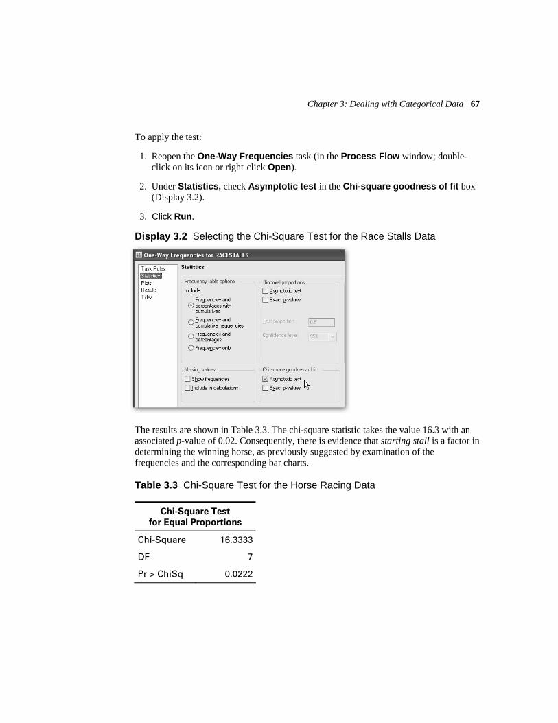
Chapter 3: Dealing with Categorical Data 67
To apply the test:
1. Reopen the One-Way Frequencies task (in the Process Flow window; double- click on its icon or right-click Open).
2. Under Statistics, check Asymptotic test in the Chi-square goodness of fit box (Display 3.2).
3. Click Run.
Display 3.2 Selecting the Chi-Square Test for the Race Stalls Data
The results are shown in Table 3.3. The chi-square statistic takes the value 16.3 with an associated p-value of 0.02. Consequently, there is evidence that starting stall is a factor in determining the winning horse, as previously suggested by examination of the frequencies and the corresponding bar charts.
Table 3.3 Chi-Square Test for the Horse Racing Data
Chi-Square Test
for Equal Proportions
Chi-Square 16.3333
DF 7
Pr > ChiSq 0.0222

68 Basic Statistics Using SAS Enterprise Guide: A Primer
3.3 Example: Brain Tumors
In an investigation of brain tumors, the type and site of the tumor for 141 individuals were noted. The three possible types were A: benign tumors, B: malignant tumors, and C: other cerebral tumors. The sites of concerned were I: frontal lobes, II: temporal lobes, and III: other cerebral areas. The data are shown in Table 3.4. Do these data give any evidence that some types of tumors occur more frequently at particular sites; i.e., that there is an association between the categorical type and site variables?
Table 3.4 Data on Type and Site of Brain Tumors
1 III A 30 III B 59 III B 88 II A 117 II B 2 III C 31 II C 60 III A 89 I A 118 III B 3 II A 32 III A 61 II A 90 III A 119 II A 4 I A 33 II A 62 III A 91 III A 120 III C 5 III A 34 II A 63 III A 92 III B 121 I C 6 III C 35 I A 64 I A 93 III C 122 I A 7 I A 36 III B 65 II C 94 I A 123 I C 8 I A 37 II B 66 III B 95 III A 124 I A 9 III A 38 II B 67 III A 96 II A 125 III A 10 III A 39 I B 68 I A 97 I B 126 III A 11 III A 40 III B 69 I A 98 II B 127 III B 12 I A 41 I C 70 II A 99 II A 128 III B 13 III A 42 I A 71 III B 100 III B 129 III A 14 III B 43 I B 72 I C 101 III B 130 III B 15 III A 44 II A 73 II A 102 III C 131 III B 16 III B 45 III B 74 III C 103 I A 132 III A 17 II A 46 II A 75 I A 104 III C 133 III C 18 III A 47 II A 76 II A 105 III A 134 III C 19 I B 48 III A 77 III A 106 III A 135 III B 20 III C 49 I B 78 III C 107 II A 136 III A 21 I A 50 III C 79 III A 108 I C 137 I A 22 III A 51 III B 80 I A 109 III A 138 I B 23 III A 52 III C 81 II A 110 III C 139 III B 24 III A 53 III A 82 I A 111 II A 140 II A 25 III A 54 I A 83 III B 112 III B 141 I A 26 III B 55 III C 84 II C 113 III C 27 III B 56 III C 85 I C 114 II A 28 II A 57 III A 86 I A 115 I B 29 I B 58 III A 87 I A 116 I B

Chapter 3: Dealing with Categorical Data 69
3.3.1 Tabulating the Brain Tumor Data into a Contingency Table
For the data about brain tumors in Table 3.4, we can cross-classify the observations to give what is know as a 3 x 3 contingency table showing the counts in all nine possible combinations of the type and site of tumors categories. The original data are in a SAS data set, tumors. Add this to the project, as above, and:
1. Select Describe Table Analysis.
2. Under Task Roles, the two variables site and type are assigned as Table variables.
3. Under Tables, drag type across to the preview pane and then site.
4. The Tables to be generated pane should now contain site by type as its first line (Display 3.3).
5. Click Run.
Display 3.3 Tables Analysis Table Preview Pane
The resulting contingency table is shown in Table 3.5.

70 Basic Statistics Using SAS Enterprise Guide: A Primer
Table 3.5 Brain Tumor Data after Cross-Classification
Table of site by type
Site Type
Frequency
Col Pct A B C Total
I 23 29.49
924.32
623.08
38
II 21 26.92
410.81
311.54
28
III 34 43.59
2464.86
1765.38
75
Total 78 37 26 141
3.3.2 Do Different Types of Brain Tumors Occur More Frequently at Particular Sites? The Chi-Square Test
We are now interested in assessing the null hypothesis that site of tumor and type of tumor are independent. Independence implies that the probabilities of the tumor types are the same at all sites. More explicitly, independence implies that the probability of a patient having a tumor of a particular type at a particular site is simply the product of the probability of this type of tumor multiplied by the probability of a tumor at this site.
We can estimate both the probability of type of tumor and the probability of a tumor at a particular site by simply dividing the appropriate marginal total by the number of observations. For example, the estimate of the probability of being a type A tumor is 78/141=0.553, and the estimate of a tumor being at site I is 38/141=0.270. So, if the null hypothesis of independence is true, then the estimate of the probability of a patient having an A type tumor at site I is 0.553 x 0.270=0.149. So, under the assumption of independence, the expected count in the type A, site I cell of the contingency table is 141 x 0.149=21.0. In the same way, we can calculate the expected values for all the other cells in the table and these can then be compared with the observed values by means of the chi-square statistic. For a contingency table with r rows and c columns, the chi-square test of independence has (r-1)(c-1) degrees of freedom where r is the number of rows of the table and c is the number of columns. In the tumor example, both r and c have the value 3 so the chi-square statistic will have four degrees of freedom. Everitt (1992) provides full details of the chi-square test of independence in contingency tables.

Chapter 3: Dealing with Categorical Data 71
The chi-square test is one of the many tests available within Table Analysis. To apply it:
1. Open the Table Analysis task (double-click or right-click Open).
2. Under Table Statistics Association, check Chi-square tests under Tests of association.
3. Click Run.
4. Replace the results from the previous run.
The result is shown in Table 3.6. Here, the chi-square test statistic takes the value 7.8 and has an associated p-value of 0.098; there is no strong evidence against the hypothesis that type and site of tumor are independent. The result implies that the observed values in Table 3.5 do not differ greatly from the corresponding values to be expected if tumor site and type of tumor are independent. Everitt (1992) describes the other terms in Table 3.6.
Table 3.6 Chi-Square Test of Independence for Brain Tumor Data
Chi-Square Tests Statistic DF Value Prob
Chi-Square 4 7.8441 0.0975
Likelihood Ratio Chi-Square 4 8.0958 0.0881
Mantel-Haenszel Chi-Square 1 2.9753 0.0845
Phi Coefficient 0.2359
Contingency Coefficient 0.2296
Cramer's V 0.1668
Sample Size = 141
3.4 Example: Suicides and Baiting Behavior
Mann (1981) reports a study carried out to investigate the causes of jeering or baiting behavior by a crowd when a person is threatening to commit suicide by jumping from a high building. A hypothesis is that baiting is more likely to occur in warm weather. Mann classified 21 accounts of threatened suicide by two factors: the time of the year and whether or not baiting occurred. The classified data are given in Table 3.7 and the question is: Do the data give any evidence to support the “warm weather” hypothesis?

72 Basic Statistics Using SAS Enterprise Guide: A Primer
(The data come from the northern hemisphere, so the months June to September are the warm months.)
Table 3.7 Crowd Behavior at Threatened Suicides
Baiting Nonbaiting
June–September 8 4 October–May 2 7
3.4.1 How Is Baiting Behavior at Suicides Affected by Season? Fisher’s Exact Test
The chi-square test carried out in the previous section for the brain tumor data above depends on knowing that the test statistic has a chi-squared distribution if the null hypothesis of independence is true; this allows p-values to be found. But what was not mentioned previously is that the chi-squared distribution is appropriate only under the assumption that the expected values are not “too small.” Such a term is almost as vague as asking how long is a piece of string, and has been interpreted in a number of ways. Most commonly, it has been taken as meaning that the chi-squared distribution is appropriate only if all the expected values are five or more. Such a “rule” is widely quoted but appears to have little mathematical or empirical justification over, say, a one-or-more rule.
Nevertheless, for contingency tables based on small sample sizes, the usual form of the chi-square test for independence may not be strictly valid although it is often difficult to predict a priori whether a given data set may cause problems. But there may be occasions where it is advisable to consider another approach that is available and that is a test that does not depend of the chi-squared distribution at all. Such exact tests of independence for a general r x c contingency table are computationally intensive and, until relatively recently, the computational difficulties have severely limited their application. But within the last ten years, the advent of fast algorithms and the availability of inexpensive computing power have considerably extended the bounds where exact test are feasible. Details of the algorithms for applying exact tests are outside the level of this text, and interested readers are referred to Mehta and Patel (1986a, 1986b) for a full exposition. But for a table in which both r and c = 2, there is an exact test which has been in use for decades, namely Fisher’s exact test, a test that is described in Everitt (1992). Fisher’s test is produced by default as part of Chi-square tests for a 2 x 2 contingency table. (For larger tables, it is available as an option.)
The data on baiting behavior at suicides provides us with an example of how to use SAS Enterprise Guide to apply Fisher’s exact test for a 2 x 2 table and will also serve to

Chapter 3: Dealing with Categorical Data 73
illustrate how to analyze data that is in the form of a table rather than individual observations. We begin by creating a new data set to enter the data into:
1. Select File New Data.
2. When prompted, type the name baiting.
A data table opens, and we enter the data with one row per cell and a column each for the number in the cell, whether or not there was baiting and whether the season was warm or cool. The columns can be renamed as baiting, season, and count, by right-clicking on the head of the column selecting properties and typing in a new name. The result should look like Display 3.4.
Display 3.4 Baiting Data Entered Directly Into SAS Enterprise Guide
Data entered in this way are stored in a temporary data set. When leaving SAS Enterprise Guide, there is the option to discard them or move them to a location where they can be retained. We have saved them to c:\saseg\sasdata.
To apply the chi-square test and Fisher’s exact test:
1. Select Describe Table Analysis.
2. Answer Yes to protect the data.
3. Under Task Roles, baiting and season are assigned as Table variables and count as a Frequency count.
4. Under Tables, drag baiting across to the preview pane and then season. The Tables to be generated pane should now contain season by baiting as its first line.
5. Under Table statistics Association, check Chi-square tests.
6. Click Run.
The crosstabulation is not reproduced exactly as entered; the categories of season and baiting are in alphabetical order. It is easier to check that the data have been correctly entered when the table is reproduced as entered. To do this, we could rerun the task and,
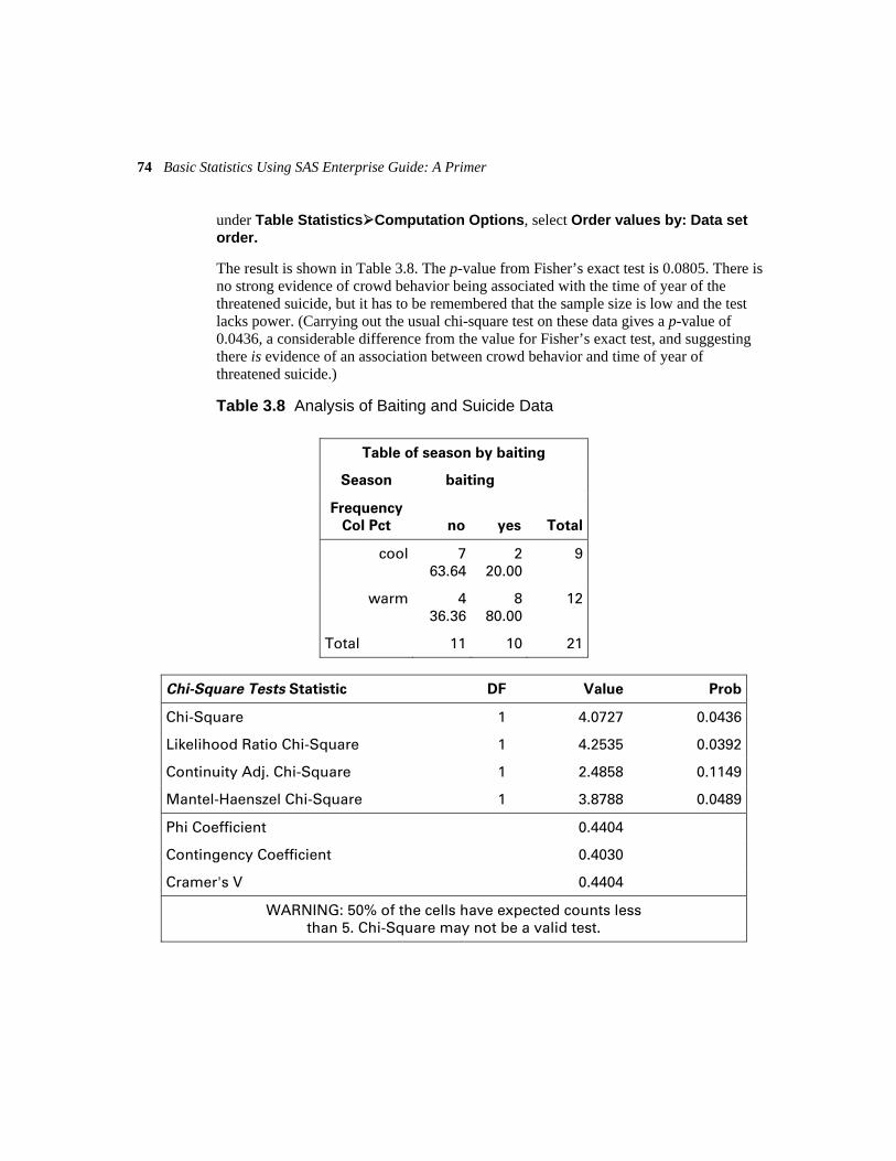
74 Basic Statistics Using SAS Enterprise Guide: A Primer
under Table Statistics Computation Options, select Order values by: Data set order.
The result is shown in Table 3.8. The p-value from Fisher’s exact test is 0.0805. There is no strong evidence of crowd behavior being associated with the time of year of the threatened suicide, but it has to be remembered that the sample size is low and the test lacks power. (Carrying out the usual chi-square test on these data gives a p-value of 0.0436, a considerable difference from the value for Fisher’s exact test, and suggesting there is evidence of an association between crowd behavior and time of year of threatened suicide.)
Table 3.8 Analysis of Baiting and Suicide Data
Table of season by baiting
Season baiting
Frequency
Col Pct no yes Total
cool 763.64
220.00
9
warm 436.36
880.00
12
Total 11 10 21
Chi-Square Tests Statistic DF Value Prob
Chi-Square 1 4.0727 0.0436
Likelihood Ratio Chi-Square 1 4.2535 0.0392
Continuity Adj. Chi-Square 1 2.4858 0.1149
Mantel-Haenszel Chi-Square 1 3.8788 0.0489
Phi Coefficient 0.4404
Contingency Coefficient 0.4030
Cramer's V 0.4404
WARNING: 50% of the cells have expected counts less than 5. Chi-Square may not be a valid test.

Chapter 3: Dealing with Categorical Data 75
Fisher's Exact Test
Cell (1,1) Frequency (F) 7
Left-sided Pr <= F 0.9942
Right-sided Pr >= F 0.0563
Table Probability (P) 0.0505
Two-sided Pr <= P 0.0805
3.5 Example: Juvenile Felons
The data in Table 3.9 (Agresti 1996) arise from a sample of juveniles convicted of felony in Florida in 1987. Matched pairs of offenders were formed using criteria such as age and number of previous offences. For each pair, one subject was handled in the juvenile court, and the other was transferred to the adult court. Whether or not the juvenile was re-arrested by the end of 1988 was then noted. Here, the question of interest in whether the population proportions re-arrested are identical for the adult and juvenile courts?
Table 3.9 Re-Arrests of Juvenile Felons by Type of Court in Which They Were Tried
Juvenile court
Adult court Re-arrest No re-arrest
Re-arrest 158 515 No re-arrest 290 1134
3.5.1 Juvenile Felons: Where Should They Be Tried? McNemar’s Test
The chi-square test on categorical data described previously assumes that the observations are independent of one another. But the data on juvenile felons in Table 3.4 arise from matched pairs and so they are not independent. The counts in the corresponding 2 x 2 table of the data refer to the pairs, so for example, in 158 of the pairs of offenders, both members of the pair were re-arrested. To test whether the re-arrest rate differs between the adult and juvenile courts, we need to apply what is known as

76 Basic Statistics Using SAS Enterprise Guide: A Primer
McNemar’s test. The test is described in Everitt (1992); to apply it to the juvenile offenders data, we can enter the data directly as with the previous example.
1. Select File New Data.
2. When prompted, supply the name arrests. A data table opens and we enter the data one row per cell and a column each for the number in the cell, the adult court outcome, and the juvenile court outcome.
3. Rename the columns as adult, juvenile, and count by right-clicking on the head of the column, selecting Column Properties, and typing in a new name. In the example below (Display 3.5), we have entered re for re-arrests and no for no re-arrests.
Display 3.5 Re-Arrest Data for Juvenile Felons Entered Directly into SAS Enterprise Guide
The data have also been stored in c:\saseg\sasdata.
To apply McNemar’s test:
1. Select Describe Table Analysis.
2. Answer Yes to protect the data.
3. Under Task Roles, adult and juvenile are assigned as Table variables and count as a Frequency count.
4. Under Tables, drag adult across to the Preview pane and then juvenile. The Tables to be generated pane should now contain juvenile by adult as its first line.
5. McNemar’s test is located under Table Statistics Agreement; check Measures.
6. To reproduce the table as entered, under Table Statistics Computation Options, set the option Order values by: to Data set order.
7. Click Run.

Chapter 3: Dealing with Categorical Data 77
The result is shown in Table 3.10. The test statistics takes the value 62.89 with an extremely small associated p-value. There is very strong evidence that type of court and the probability of re-arrest are related. It appears that trial at a juvenile court is less likely to result in re-arrest.
Table 3.10 McNemar’s Test for Juvenile Crime Data
Table of adult by juvenile
adult juvenile
Frequency
Col Pct re no Total
re 15835.27
51531.23
673
no 29064.73
113468.77
1424
Total 448 1649 2097
McNemar's Test
Statistic (S) 62.8882
DF 1
Pr > S <.0001
3.6 Exercises
Exercise 3.1 The crash data set lists fictitious counts of fatal air crashes in Australia by quarter over a twenty-year period. Assess the hypothesis that the accident rates are uniform across these four quarters:
Jan April July October
12 8 7 8
Exercise 3.2 One hundred American citizens were surveyed and asked to identify which of five items were most fearful to them. The results are given in the fear data set. Test whether sex and greatest fear are independent of each other.
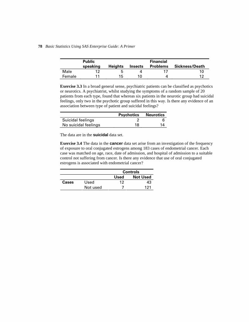
78 Basic Statistics Using SAS Enterprise Guide: A Primer
Public
speaking
Heights
Insects
Financial
Problems
Sickness/Death
Male 12 5 4 17 10 Female 11 15 10 4 12
Exercise 3.3 In a broad general sense, psychiatric patients can be classified as psychotics or neurotics. A psychiatrist, whilst studying the symptoms of a random sample of 20 patients from each type, found that whereas six patients in the neurotic group had suicidal feelings, only two in the psychotic group suffered in this way. Is there any evidence of an association between type of patient and suicidal feelings?
Psychotics Neurotics
Suicidal feelings 2 6No suicidal feelings 18 14
The data are in the suicidal data set.
Exercise 3.4 The data in the cancer data set arise from an investigation of the frequency of exposure to oral conjugated estrogens among 183 cases of endometrial cancer. Each case was matched on age, race, date of admission, and hospital of admission to a suitable control not suffering from cancer. Is there any evidence that use of oral conjugated estrogens is associated with endometrial cancer?
Controls
Used Not Used
Used 12 43Cases
Not used 7 121
C h a p t e r 4
Dealing with Bivariate Data
4.1 Introduction 80 4.2 Example: Heights and Resting Pulse Rates 80
4.2.1 Plotting Heights and Resting Pulse Rates: The Scatterplot 81 4.2.2 Quantifying the Relationship between Resting Pulse Rate and Height:
The Correlation Coefficient 82 4.2.3 Heights and Resting Pulse Rates: Simple Linear Regression 85
4.3 Example: An Experiment in Kinesiology 90 4.3.1 Oxygen Uptake and Expired Ventilation: The Scatterplot 91 4.3.2 Expired Ventilation and Oxygen Uptake: Is Simple Linear Regression
Appropriate? 93 4.4 Example: U.S. Birthrates in the 1940s 95
4.4.1 Plotting the Birthrate Data: The Aspect Ratio of a Scatterplot 95 4.5 Exercises 102

80 Basic Statistics Using SAS Enterprise Guide: A Primer
4.1 Introduction
When two observations or measurements are made on each member of a sample, we have what is generally termed bivariate data. In this chapter, we shall show how to construct informative graphical displays of such data and how to quantify the relationship between the two variables in such data sets. The statistical topics to be covered in this chapter are:
Plotting the data—Scatterplots
Assessing strength of linear relationship—Correlation coefficients
Fitting a line to the data—Simple linear regression
4.2 Example: Heights and Resting Pulse Rates
The data in Table 4.1 show the heights (in centimeters) and resting pulse rates (beats per minute) for a sample of hospital patients. The main question of interest is whether there is any relationship between height and pulse rate.
Table 4.1 Heights (Cm) and Resting Pulse (Bpm) Data
160 68 160 78 185 80 160 80 167 80 170 90 163 95 182 80 162 84 177 80 177 80 168 80 175 80 166 72 165 76 155 80 185 80 170 80 182 100 175 104 162 80 148 82 162 88 168 80 173 92 175 76 172 90 180 68 167 92 160 84 177 90 175 84 170 80 153 70 168 90 145 64 170 80 185 80 178 80 170 84 163 80 165 82 182 76 175 72 158 80 165 84 167 80
157 80 172 116 170 84
Chapter 4: Dealing with Bivariate Data 81
4.2.1 Plotting Heights and Resting Pulse Rates: The Scatterplot
The height and resting pulse data set is called bivariate since two variables are measured for each individual. The separate variables in the data set can, of course, each be summarized and graphed using the methods described in Chapter 2. Of more importance and more interest for bivariate data is to describe and graph the data in a way that lends insights as to how the two variables are related. Let’s begin by looking at the most commonly used graphic for bivariate data namely the scatterplot—an xy plot of the two variables which has been in use since at least the 18th century and has many virtues; indeed, according to Tufte (1983):
The relational graphic—in its barest form the scatterplot and its variants—is the greatest of all graphical designs. It links at least two variables encouraging and even imploring the viewer to assess the possible causal relationship between the plotted variables. It confronts causal theories that x causes y with empirical evidence as to the actual relationship between x and y.
The data giving heights and resting pulse rates shown in Table 4.1 are already available in a SAS data set, resting. As in the previous chapter, we will keep the analysis of each data set separate by creating a process flow window for each. So, before adding the data set, we rename the default process flow to resting, by right-clicking on the Process Flow tab and selecting Rename. Then, we add the data set to the process flow.
1. Select File Open Data Local Computer.
2. Browse to the folder containing the SAS data sets (c:\saseg\sasdata).
3. Select the file and click Open.
For the scatterplot:
1. Select Graph Scatter Plot.
2. Under Scatter Plot, select 2D Scatter Plot.
3. Under Task Roles, drag height to Horizontal and pulse to Vertical.
4. Click Run.
The resulting plot is shown in Figure 4.1 and suggests that increasing height is generally (although not universally) associated with an increase in resting pulse, and that the relationship between the two variables is, approximately at least, linear; i.e., it can be described by a straight line (see Section 4.2.3).

82 Basic Statistics Using SAS Enterprise Guide: A Primer
Figure 4.1 Scatterplot of Pulse against Height
4.2.2 Quantifying the Relationship between Resting Pulse Rate and Height: The Correlation Coefficient
How can we summarize and quantify any relationship between two variables indicated in the scatterplot of the two variables in a single number? What is needed is to measure the correlation between the two variables using a correlation coefficient. For two continuous variables, we can use Pearson’s correlation coefficient, also known as the product-moment correlation coefficient.
The product moment correlation coefficient is the ratio of the sum of products of differences of each variable from its mean divided by the square roots of the two sums of squares about the mean. Altman (1991) includes more details of how the coefficient is calculated. The product moment coefficient takes values between –1 and 1. Negative values indicate that large values of x are associated with small values of y and vice versa. Positive values indicate the reverse. The correlation coefficient has a maximum value of

Chapter 4: Dealing with Bivariate Data 83
+1 when the points in the scatterplot all lie exactly on a straight line and the variables are positively correlated. The correlation coefficient has a minimum value of –1 when all the points lie exactly on a straight line and the variables are negatively correlated. When the correlation coefficient is zero, the variables are said to be uncorrelated.
In essence, the correlation coefficient is a measure of how closely the points in the scatterplot are to a straight line; it measures the linear relationship between two variables; nonlinear relationships may be missed or underestimated by it. For example, Figure 4.2 shows a perfect nonlinear relationship between two variables for which the correlation coefficient takes the value 0, and Figure 4.3 shows another perfect nonlinear relationship for which the coefficient is not 1. The examples in Figures 4.2 and 4.3 demonstrate the need to use the scatterplot alongside the correlation coefficient when assessing relationships between variables. Use of the correlation coefficient alone is insufficient and can lead to misinterpretation of the data.
Figure 4.2 Perfect Nonlinear Relationship between Two Variables for Which the Correlation Coefficient Is Almost Zero

84 Basic Statistics Using SAS Enterprise Guide: A Primer
Figure 4.3 Perfect Nonlinear Relationship between Two Variables for Which the Correlation Coefficient Is Nevertheless Not One
To calculate the product moment correlation coefficients for height and resting pulse rate data:
1. Select the resting data set.
2. Select Analyze Multivariate Correlations.
3. Under Task Roles, assign both variables to be Analysis variables.
4. Click Run.
The results are shown in Table 4.2.
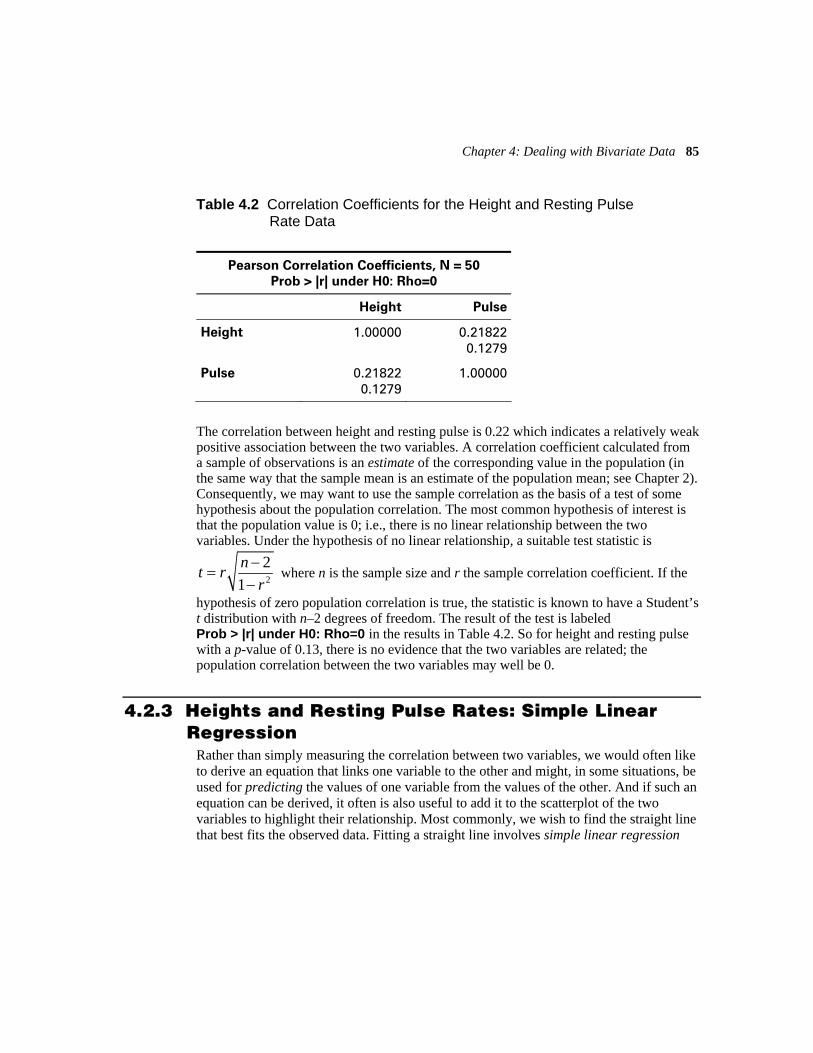
Chapter 4: Dealing with Bivariate Data 85
Table 4.2 Correlation Coefficients for the Height and Resting Pulse Rate Data
Pearson Correlation Coefficients, N = 50
Prob > |r| under H0: Rho=0
Height Pulse
Height 1.00000 0.218220.1279
Pulse 0.218220.1279
1.00000
The correlation between height and resting pulse is 0.22 which indicates a relatively weak positive association between the two variables. A correlation coefficient calculated from a sample of observations is an estimate of the corresponding value in the population (in the same way that the sample mean is an estimate of the population mean; see Chapter 2). Consequently, we may want to use the sample correlation as the basis of a test of some hypothesis about the population correlation. The most common hypothesis of interest is that the population value is 0; i.e., there is no linear relationship between the two variables. Under the hypothesis of no linear relationship, a suitable test statistic is
2
21nt r
r−
=−
where n is the sample size and r the sample correlation coefficient. If the
hypothesis of zero population correlation is true, the statistic is known to have a Student’s t distribution with n–2 degrees of freedom. The result of the test is labeled Prob > |r| under H0: Rho=0 in the results in Table 4.2. So for height and resting pulse with a p-value of 0.13, there is no evidence that the two variables are related; the population correlation between the two variables may well be 0.
4.2.3 Heights and Resting Pulse Rates: Simple Linear Regression
Rather than simply measuring the correlation between two variables, we would often like to derive an equation that links one variable to the other and might, in some situations, be used for predicting the values of one variable from the values of the other. And if such an equation can be derived, it often is also useful to add it to the scatterplot of the two variables to highlight their relationship. Most commonly, we wish to find the straight line that best fits the observed data. Fitting a straight line involves simple linear regression

86 Basic Statistics Using SAS Enterprise Guide: A Primer
and least squares estimation, both of which are described in detail in Altman (1991). But essentially we postulate the following model for the data and then estimate the model’s two parameters α (the intercept of the line) and β (the slope of the line):
i i iy xα β ε= + +
In the model above, ,i ix y represent the observed values of the two variables for the ith subject in the sample of observations, and iε represents the error; i.e., the amount by which iy differs from its value as predicted by the model, namely ixα β+ . The formulae for the sample estimates of and α β are given explicitly in Altman (1991).
We can fit the simple linear regression model to the heights and resting pulse rate data as follows:
1. Select the resting data set.
2. Select Analyze Regression Linear.
3. Under Task Roles, assign pulse the role of Dependent variable and height the role of Explanatory variables (Display 4.1). Note that there is no distinction between Quantitative and Classification variables. In the Linear Regression task, all explanatory variables are assumed to be quantitative.
4. Click Run.

Chapter 4: Dealing with Bivariate Data 87
Display 4.1 Task Roles Pane for Linear Regression of Resting Pulse Data
The results are shown in Table 4.3.

88 Basic Statistics Using SAS Enterprise Guide: A Primer
Table 4.3 Results of Fitting a Simple Linear Regression Model to the Height and Pulse Rate Data
Number of Observations Read 50
Number of Observations Used 50
Analysis of Variance
Source DF
Sum of
Squares
Mean
Square F Value Pr > F
Model 1 186.32129 186.32129 2.40 0.1279
Error 48 3726.17871 77.62872
Corrected Total 49 3912.50000
Root MSE 8.81072 R-Square 0.0476
Dependent Mean 82.30000 Adj R-Sq 0.0278
Coeff Var 10.70561
Parameter Estimates
Variable DF
Parameter
Estimate
Standard
Error t Value Pr > |t|
Intercept 1 46.90693 22.87933 2.05 0.0458
height 1 0.20977 0.13540 1.55 0.1279
The first part of Table 4.3 gives an analysis of variance table (see Chapter 5) in which the variation in the y variable is partitioned into a part due to the fitted model and a part due to the error term in the model. The associated F-test (see Chapter 5) gives a test of the hypothesis that the population value of the slope is 0 ( 0H : 0β = ). Here, the p-value associated with the F-test is 0.13 so there is no evidence for a non-zero slope. (Note that the p-value is the same as the previously described test for zero correlation between the two variables; the two tests are, of course, equivalent.)

Chapter 4: Dealing with Bivariate Data 89
The most important term in the second part of Table 4.4 is R-square which is the square of the correlation between the observed values of the response variable, and the values of the response variable predicted by the fitted model. R-square gives the variance in the response variable y that is explained by the x variable. Here, the R-square value of 0.0476 shows that only about 5% of the variance in pulse rate is accounted for by height. The last section of Table 4.3 gives the estimated intercept and slope for the model. The slope is estimated to be 0.21 which implies that, for every centimeter increase in height, pulse rate increases by 0.21. But since the standard error of the estimated slope is 0.14, the 95% confidence interval for the slope is [–0.07,0.49] which includes the value zero, as we already knew it would from the result of the F-test discussed above.
To add the fitted line and confidence limits for the line to the scatterplot of the two variables, proceed as follows:
1. Reopen the Linear Regression task (double-click or right-click Open).
2. Under Plots Predicted, select Observed vs independents and Confidence limits (Display 4.2).
3. Click Run.
4. Replace previous results.
The resulting plot is shown in Figure 4.4. We can see that a horizontal line (i.e., one with slope zero) could easily be fitted between the two confidence limits.
Display 4.2 Selecting Plots of Predicted Values for the Resting Pulse Data
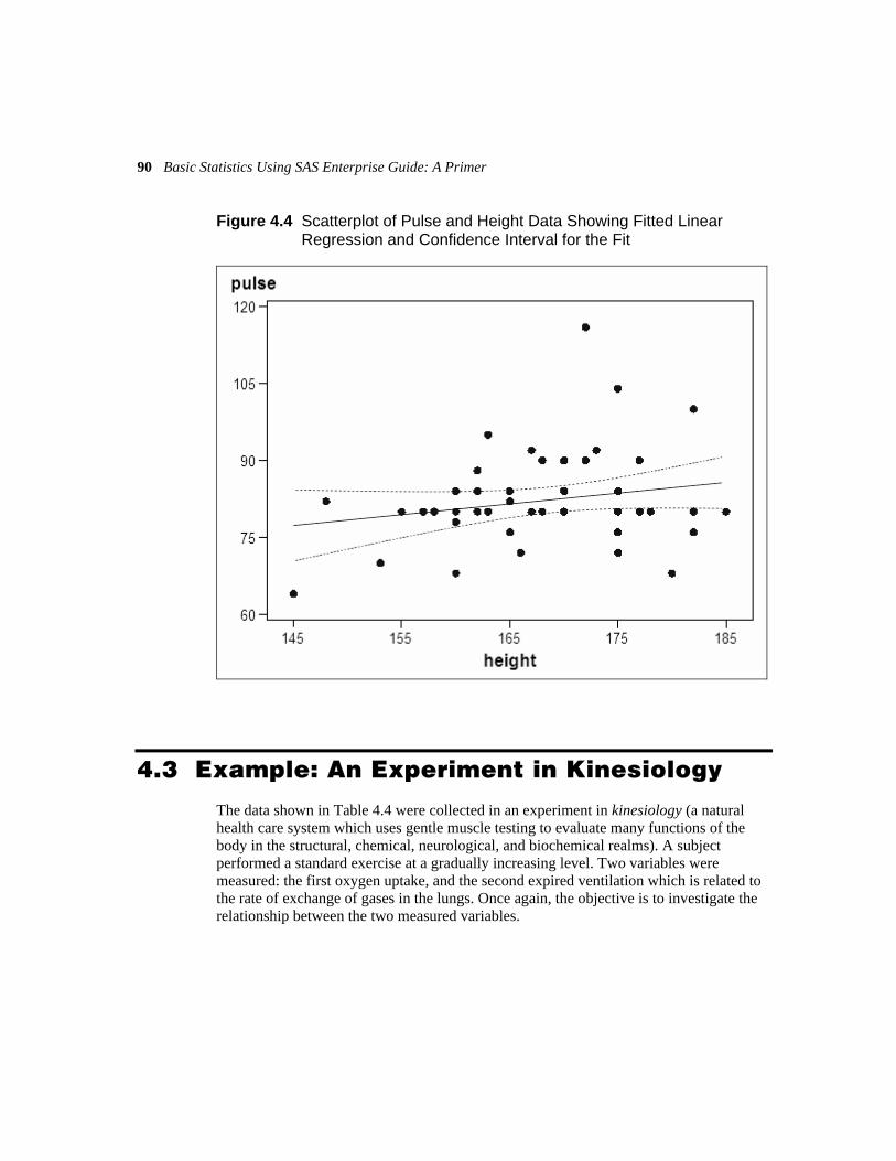
90 Basic Statistics Using SAS Enterprise Guide: A Primer
Figure 4.4 Scatterplot of Pulse and Height Data Showing Fitted Linear Regression and Confidence Interval for the Fit
4.3 Example: An Experiment in Kinesiology
The data shown in Table 4.4 were collected in an experiment in kinesiology (a natural health care system which uses gentle muscle testing to evaluate many functions of the body in the structural, chemical, neurological, and biochemical realms). A subject performed a standard exercise at a gradually increasing level. Two variables were measured: the first oxygen uptake, and the second expired ventilation which is related to the rate of exchange of gases in the lungs. Once again, the objective is to investigate the relationship between the two measured variables.

Chapter 4: Dealing with Bivariate Data 91
Table 4.4 Oxygen Uptake and Expired Ventilation Data
574 21.9 1639 29.2 2766 55.8 3844 100.9 592 18.6 1787 32.0 2812 54.5 3878 103.0 664 18.6 1790 27.9 2893 63.5 4002 113.4 667 19.1 1794 31.0 2957 60.3 4114 111.4 718 19.2 1874 30.7 3052 64.8 4152 119.9 770 16.9 2049 35.4 3151 69.2 4252 127.2 927 18.3 2132 36.1 3161 74.7 4290 126.4 947 17.2 2160 39.1 3266 72.9 4331 135.5 1020 19.0 2292 42.6 3386 80.4 4332 138.9 1096 19.0 2312 39.9 3452 83.0 4390 143.7 1277 18.6 2475 46.2 3521 86.0 4393 144.8 1323 22.8 2489 50.9 3543 88.9 1330 24.6 2490 46.5 3676 96.8 1599 24.9 2577 46.3 3741 89.1
4.3.1 Oxygen Uptake and Expired Ventilation: The Scatterplot
The data on oxygen uptake and expired ventilation, shown in Table 4.2, are also available in a SAS data set, anaerob. Before adding them, we create a new process flow window (File New Process Flow) and rename it anaerob. Then, we add the data to it in the same way as for the resting data set in the previous section. Repeat the scatterplot task assigning o2in to the horizontal axis and airout to the vertical axis. The result is shown in Figure 4.5, which clearly demonstrates that there is a strong relationship between oxygen uptake and expired ventilation, but that this relationship is distinctly nonlinear; as oxygen uptake increases, expired ventilation accelerates making the relationship between the two variables depart from a straight line form.

92 Basic Statistics Using SAS Enterprise Guide: A Primer
Figure 4.5 Scatterplot of Oxygen Uptake and Expired Ventilation
The correlation coefficient for oxygen uptake and expired ventilation can be found in the same way as described in the previous section for height and resting pulse rate. The results are shown in Table 4.5.
Table 4.5 Correlation for Oxygen Uptake and Expired Ventilation
Pearson Correlation Coefficients, N = 53
Prob > |r| under H0: Rho=0
o2in Airout
o2in Oxygen uptake
1.00000 0.95498<.0001
airout Expired ventilation
0.95498<.0001
1.00000

Chapter 4: Dealing with Bivariate Data 93
For oxygen uptake and expired volume, the correlation is 0.95. Since we know the relationship to be nonlinear, use of the coefficient is not totally informative about the nature of the data and so, although a very small p-value associated with the test of zero correlation provides strong evidence that the two variables are related, the scatterplot indicates that the relationship is not linear. This example emphasizes that it is generally good practice to always have the scatterplot of two variables visible when trying to interpret the correlation coefficient between them.
4.3.2 Expired Ventilation and Oxygen Uptake: Is Simple Linear Regression Appropriate?
We can repeat what was done in the previous subsection for the expired ventilation and oxygen uptake data to give Table 4.6 and Figure 4.6. Here, the test for a zero slope has a very small associated p-value; there is strong evidence that the slope is not zero. The R-square value shows that 91% of the variation in expired ventilation can be attributed to variation in oxygen uptake. But the plot in Figure 4.6 shows that, despite the seemingly impressive statements about the linear fit, it is not the correct model for the ventilation/oxygen data; readers are advised to carry out Exercise 4.3 and fit a more appropriate model for the data.
Table 4.6 Results of Fitting a Linear Regression Model to the Expired Ventilation and Oxygen Uptake Data
Number of Observations Read 53
Number of Observations Used 53
Analysis of Variance
Source DF
Sum of
Squares
Mean
Square F Value Pr > F
Model 1 75555 75555 528.40 <.0001
Error 51 7292.38118 142.98787
Corrected Total 52 82848

94 Basic Statistics Using SAS Enterprise Guide: A Primer
Root MSE 11.95775 R-Square 0.9120
Dependent Mean 60.70755 Adj R-Sq 0.9103
Coeff Var 19.69731
Parameter Estimates
Variable Label DF
Parameter
Estimate
Standard
Error t Value Pr > |t|
Intercept Intercept 1 -18.44873 3.81520 -4.84 <.0001
o2in Oxygen uptake
1 0.03114 0.00135 22.99 <.0001
Figure 4.6 Plot of Expired Ventilation and Oxygen Uptake Data Showing Fitted Linear Regression and Its Confidence Limits
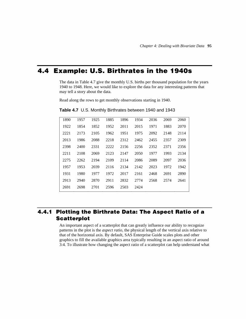
Chapter 4: Dealing with Bivariate Data 95
4.4 Example: U.S. Birthrates in the 1940s
The data in Table 4.7 give the monthly U.S. births per thousand population for the years 1940 to 1948. Here, we would like to explore the data for any interesting patterns that may tell a story about the data.
Read along the rows to get monthly observations starting in 1940.
Table 4.7 U.S. Monthly Birthrates between 1940 and 1943
1890 1957 1925 1885 1896 1934 2036 2069 2060
1922 1854 1852 1952 2011 2015 1971 1883 2070
2221 2173 2105 1962 1951 1975 2092 2148 2114
2013 1986 2088 2218 2312 2462 2455 2357 2309
2398 2400 2331 2222 2156 2256 2352 2371 2356
2211 2108 2069 2123 2147 2050 1977 1993 2134
2275 2262 2194 2109 2114 2086 2089 2097 2036
1957 1953 2039 2116 2134 2142 2023 1972 1942
1931 1980 1977 1972 2017 2161 2468 2691 2890
2913 2940 2870 2911 2832 2774 2568 2574 2641
2691 2698 2701 2596 2503 2424
4.4.1 Plotting the Birthrate Data: The Aspect Ratio of a Scatterplot
An important aspect of a scatterplot that can greatly influence our ability to recognize patterns in the plot is the aspect ratio, the physical length of the vertical axis relative to that of the horizontal axis. By default, SAS Enterprise Guide scales plots and other graphics to fill the available graphics area typically resulting in an aspect ratio of around 3:4. To illustrate how changing the aspect ratio of a scatterplot can help understand what

96 Basic Statistics Using SAS Enterprise Guide: A Primer
the data might be trying to tell us, we shall use the birthrate data given in Table 4.7. First, we create a new process flow window:
1. Select File New Process Flow.
2. Rename it to usbirths (right-click on the Process Flow tab Rename).
The data are in a file usbirths.dat in the data directory (c:\saseg\data). Import them to the project.
1. Select File Import Data.
2. Select Local Computer, navigate to the location of the file, and click Open. There is only a single column of data, so the default import options will suffice.
3. Under Column Options, rename the column to births.
4. Click Run.
The timing of the data is implicit in the order. To create a variable to represent this information:
1. Select Analyze Time Series Prepare Time Series Data.
2. Under Task Roles, drag New TimeId to Time ID variable and rename it month.
3. Monthly is the default interval, so set the staring date to 1/1/1940. The screen should now look like Display 4.3.
4. Click Run.

Chapter 4: Dealing with Bivariate Data 97
Display 4.3 Preparing Time Series of U.S. Births Data: Task Roles Pane
We can construct a scatterplot of the birthrates against month with the default aspect ratio:
1. Select Graph Scatter Plot.
2. Under Task Roles, assign births to Vertical and month to Horizontal.
3. Click Run.
The resulting plot is shown in Figure 4.7. The plot shows that the U.S. birthrate was increasing between 1940 and 1943, decreasing between 1943 and 1946, rapidly increasing during 1946, and then decreasing again during 1947–1948. As Cook and Weisberg (1982) comment:
These trends seem to deliver an interesting history lesson since the U.S. involvement in World War II started in 1942 and troops began returning home during the part of 1945, about nine months before the rapid increase in the birthrate.

98 Basic Statistics Using SAS Enterprise Guide: A Primer
Figure 4.7 Scatterplot of Birthrate V Month
Now let’s see what happens when we alter the aspect ratio of the plot:
1. Reopen the Scatter Plot task (double-click or right-click Open).
2. Under Appearance Chart Area, select Specify custom chart size, and enter 600 for Width and 200 for Height.
3. Under Appearance Plots, reduce the size of the data point marker to around a third (3 points).
4. Click Run.
5. Do not replace the previous results.
The resulting graph appears in Figure 4.8.

Chapter 4: Dealing with Bivariate Data 99
Figure 4.8 Scatterplot of Birthrate V Month with Aspect Ratio 0.3
The new plot displays many peaks and troughs and suggests perhaps some minor within-year trends in addition to the global trends apparent in Figure 4.7.
A clearer picture is obtained by plotting only a part of the data; here, we will plot the observations for the years 1940–1943. To do this, we begin by creating a filter to include only data for the years 1940–1943:
1. Select the data set (click on the icon labeled Modified Time Series data for SASUSER.IMPW).
2. Select Data Filter and Query. This opens the Query Builder window.
3. Under the Filter Data tab, drag and drop month.
4. The Edit Filter window opens. Change Operator to Less than; click the drop-down button next to the Value box, and click Get Values in the pop-up window.
5. From the list that appears, select ‘1Jan1944’d.
6. Click OK (see Display 4.4).
7. Click Run.

100 Basic Statistics Using SAS Enterprise Guide: A Primer
Display 4.4 Filter Data Pane: Selecting Data Prior to 1944
The results are displayed showing only observations for 1940–1943. Select (click) this data set in the Process Flow window and then construct a scatterplot of births by month using the same options as for Figure 4.7. The result is shown in Figure 4.9.
Figure 4.9 Scatterplot of Birthrate V Month for Years 1940–1943; Aspect Ratio=0.3
Now, a within-year cycle is clearly apparent with the lowest within-year birthrate at the beginning of the summer and the highest birthrate occurring in the autumn. This pattern can be made clearer in a line plot with the same options as Figure 4.7.

Chapter 4: Dealing with Bivariate Data 101
1. Select Graph Line Plot.
2. Under Line Plot, the default, simply labeled Line Plot, is the type we want. Double-click Line Plot.
3. Under Task Roles, assign births to Vertical and month to Horizontal.
4. Under Appearance Chart Area, select Specify custom chart size, and enter 600 for Width and 200 for Height.
5. Click Run.
The new plot appears in Figure 4.10.
Figure 4.10 Scatterplot of Birthrate V Month for Years 1940–1943 with Observations Joined and Aspect Ratio=0.3
By reducing the aspect ratio to 0.25 and replotting all 96 observations with a line plot, both the within-year and global trends become clearly visible. Select the full data set (click on the icon labeled Modified Time Series data for SASUSER.IMPW), then run the Line Plot task for month and births with the Chart Area set to 600 by 150.
The result is shown in Figure 4.11.
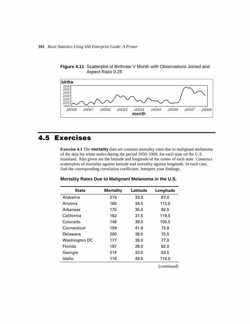
102 Basic Statistics Using SAS Enterprise Guide: A Primer
Figure 4.11 Scatterplot of Birthrate V Month with Observations Joined and Aspect Ratio 0.25
4.5 Exercises
Exercise 4.1 The mortality data set contains mortality rates due to malignant melanoma of the skin for white males during the period 1950–1969, for each state on the U.S. mainland. Also given are the latitude and longitude of the center of each state. Construct scatterplots of mortality against latitude and mortality against longitude. In each case, find the corresponding correlation coefficient. Interpret your findings.
Mortality Rates Due to Malignant Melanoma in the U.S.
State Mortality Latitude Longitude
Alabama 219 33.0 87.0 Arizona 160 34.5 112.0
Arkansas 170 35.0 92.5 California 182 37.5 119.5
Colorado 149 39.0 105.5 Connecticut 159 41.8 72.8
Delaware 200 39.0 75.5 Washington DC 177 39.0 77.0
Florida 197 28.0 82.0 Georgia 214 33.0 83.5
Idaho 116 44.5 114.0
(continued)
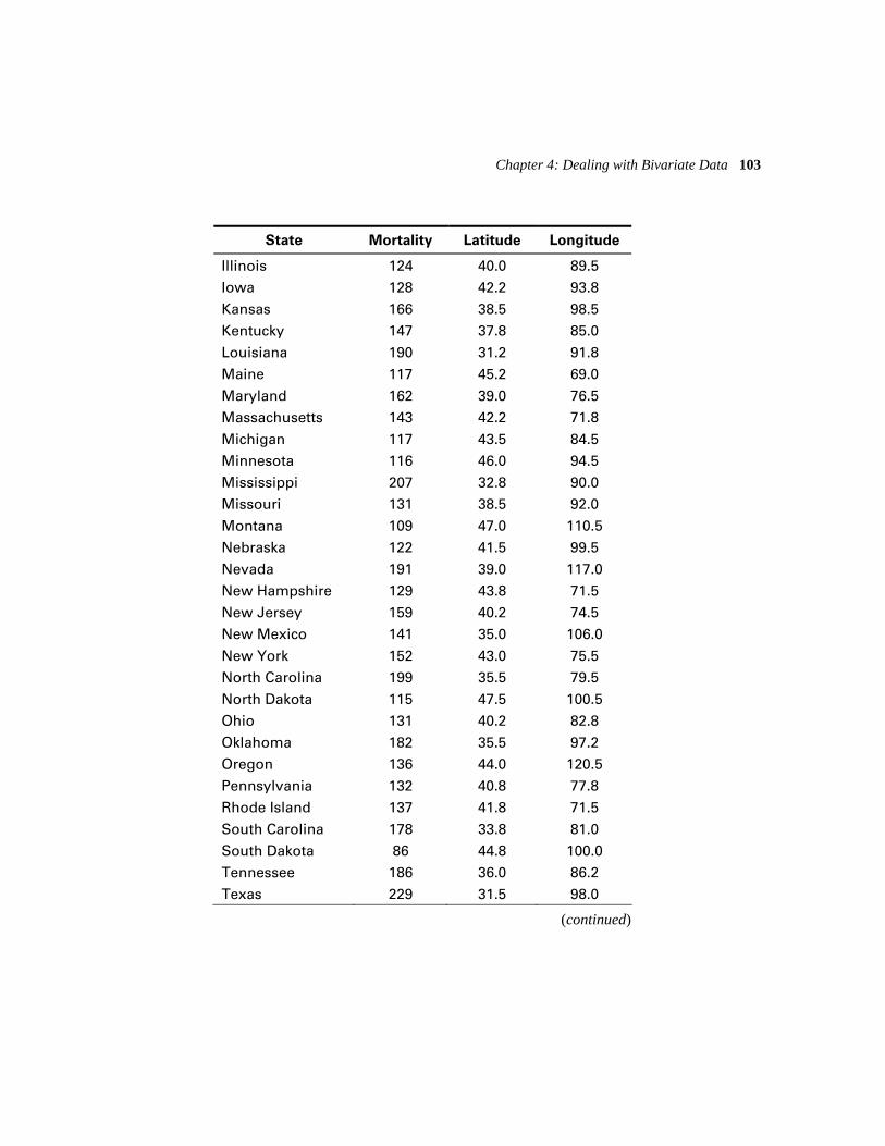
Chapter 4: Dealing with Bivariate Data 103
State Mortality Latitude Longitude
Illinois 124 40.0 89.5 Iowa 128 42.2 93.8
Kansas 166 38.5 98.5 Kentucky 147 37.8 85.0
Louisiana 190 31.2 91.8 Maine 117 45.2 69.0
Maryland 162 39.0 76.5 Massachusetts 143 42.2 71.8
Michigan 117 43.5 84.5 Minnesota 116 46.0 94.5
Mississippi 207 32.8 90.0 Missouri 131 38.5 92.0
Montana 109 47.0 110.5 Nebraska 122 41.5 99.5
Nevada 191 39.0 117.0 New Hampshire 129 43.8 71.5
New Jersey 159 40.2 74.5 New Mexico 141 35.0 106.0
New York 152 43.0 75.5 North Carolina 199 35.5 79.5
North Dakota 115 47.5 100.5 Ohio 131 40.2 82.8
Oklahoma 182 35.5 97.2 Oregon 136 44.0 120.5
Pennsylvania 132 40.8 77.8 Rhode Island 137 41.8 71.5
South Carolina 178 33.8 81.0 South Dakota 86 44.8 100.0
Tennessee 186 36.0 86.2 Texas 229 31.5 98.0
(continued)

104 Basic Statistics Using SAS Enterprise Guide: A Primer
State Mortality Latitude Longitude
Utah 142 39.5 111.5 Vermont 153 44.0 72.5
Virginia 166 37.5 78.5 Washington 117 47.5 121.0
West Virginia 136 38.8 80.8 Wisconsin 110 44.5 90.2
Wyoming 134 43.0 107.5
Exercise 4.2 Construct a scatterplot of the data in expired ventilation and oxygen uptake data in Table 4.2. Add the fitted quadratic curve to the plot; i.e., a curve of the form
21 2i i i iy x xα β β ε= + + +
Exercise 4.3 The index data set gives the values of a food price index and a house price measure for the U.K. for each year from 1971 to 1989. By constructing suitable plots, investigate how the two price measures change over time, and how the changes are related. (Experiment with changing the aspect ratio of the plots you create.)
Year Food index House Index
1971 155.6 60 1972 169.4 79 1973 194.9 107
1974 230.0 113 1975 288.9 124
1976 346.5 134 1977 412.4 148
1978 441.6 177 1979 494.7 227
1980 554.5 272 1981 601.3 280
1982 648.6 285 1983 669.2 317
(continued)

Chapter 4: Dealing with Bivariate Data 105
Year Food index House Index
1984 706.7 342 1985 728.8 373
1986 752.6 436 1987 775.6 513
1988 802.4 646 1989 847.7 750

106 Basic Statistics Using SAS Enterprise Guide: A Primer

C h a p t e r 5
Analysis of Variance
5.1 Introduction 108 5.2 Example: Teaching Arithmetic 108
5.2.1 Initial Examination of the Teaching Arithmetic Data with Summary
Statistics and Box Plots 109 5.2.2 Teaching Arithmetic: Are Some Teaching Methods for Teaching
Arithmetic Better Than Others? 112 5.3 Example: Weight Gain in Rats 116
5.3.1 A First Look at the Rat Weight Gain Data Using Box Plots and
Numerical Summaries 116 5.3.2 Weight Gain in Rats: Do Rats Gain More Weight on a Particular
Diet? 119 5.4 Example: Mother’s Post-Natal Depression and Child’s IQ 124
5.4.1 Summarizing the Post-Natal Depression Data 125 5.4.2 How Is a Child’s IQ Affected by Post-Natal Depression in the
Mother? 128 5.5 Exercises 133

108 Basic Statistics Using SAS Enterprise Guide: A Primer
5.1 Introduction
In this chapter, we will describe how to analyze data in which a response variable of interest is measured in different levels of one or more categorical factor variables. The statistical topics to be covered are:
Analysis of variance for the one way design
Factorial designs, balanced and unbalanced
Type I and Type III sums of squares
Multiple comparison tests
5.2 Example: Teaching Arithmetic
In an experiment to compare different methods of teaching arithmetic (Wetherill 1982), 45 students were divided randomly into five groups of equal size. Two groups—1 and 2—were taught by the current method, and three—3, praised; 4, reproved; 5, ignored— were taught by one of three new methods. At the end of the investigation, all pupils took a standard test with the results shown in Table 5.1. What conclusions can be drawn about possible differences between teaching methods?
Table 5.1 Data on Teaching Methods
Teaching
method
Test
results
1 17,14,24,20,24,23,16,15,24 2 21,23,13,19,13,19,20,21,16
3 28,30,29,24,27,30,28,28,23 4 19,28,26,26,19,24,24,23,22
5 21,14,13,19,15,15,10,18,20
Before beginning any formal analysis of the data sets in the previous section, it will be useful to consider some summary statistics and graphics for the data since both will be helpful in both gaining informal insights into the data and aiding the interpretation of the formal testing to be described later.

Chapter 5: Analysis of Variance 109
5.2.1 Initial Examination of the Teaching Arithmetic Data with Summary Statistics and Box Plots
The teaching data in Table 5.1 are already available in a SAS data set, teaching. Add the data set to the project:
1. Select File Open Data Local Computer.
2. Browse to the folder containing the SAS data set (c:\saseg\sasdata).
3. Select the file.
4. Click Open.
We saw in Chapter 3 how to produce tables of counts and percentages. Here, we need tables containing other summary statistics, specifically means and standard deviations. To do this:
1. Select Describe Summary Tables.
2. Under Task Roles, classification variables are those whose values will be used to form the rows and/or columns of the table, and analysis variables are those whose values are to be summarized within the table. In this case, method is a Classification variable and result is an Analysis variable.
3. Under Summary Tables, tables are constructed by dragging variables across to the appropriate position in the Preview pane. If a variable is not appropriate for the position it is dragged to, the cursor will change to a stop sign ( ).
4. Drag method to the row position (left side). A column headed N appears. This is because the default summary statistic for Classification variables is a count.
5. Drag result to the column position on either edge of the box containing N. Sum appears below it, as this is the default summary statistic for an Analysis variable.
6. From the Available statistics pane, drag mean to the left edge of the N box.
7. Repeat Step 6 with stdev (standard deviation).
8. Remove Sum by dragging it off the Preview pane.
9. Among the Available variables there is an additional variable, All. This is used to form totals. Drag it to the bottom edge of the method box. The Summary Tables pane should now look like the example in Display 5.1.
10. Click Run.

110 Basic Statistics Using SAS Enterprise Guide: A Primer
The results are shown in Table 5.2.
Display 5.1 Summary Tables Pane for the Teaching Data
Table 5.2 Summary Statistics for Teaching Methods Data
result
Mean StdDev N
Method
1 19.67 4.21 9
2 18.33 3.57 9
3 27.44 2.46 9
4 23.44 3.09 9
5 16.11 3.62 9
All 21.00 5.21 45
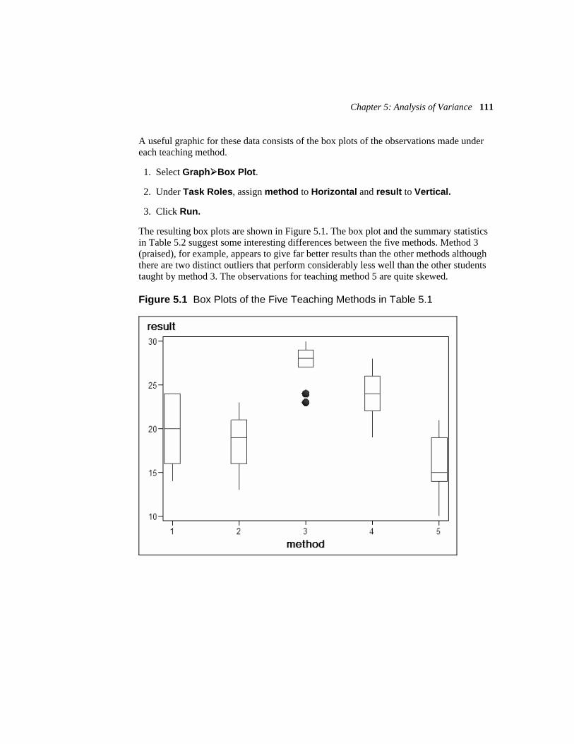
Chapter 5: Analysis of Variance 111
A useful graphic for these data consists of the box plots of the observations made under each teaching method.
1. Select Graph Box Plot.
2. Under Task Roles, assign method to Horizontal and result to Vertical.
3. Click Run.
The resulting box plots are shown in Figure 5.1. The box plot and the summary statistics in Table 5.2 suggest some interesting differences between the five methods. Method 3 (praised), for example, appears to give far better results than the other methods although there are two distinct outliers that perform considerably less well than the other students taught by method 3. The observations for teaching method 5 are quite skewed.
Figure 5.1 Box Plots of the Five Teaching Methods in Table 5.1

112 Basic Statistics Using SAS Enterprise Guide: A Primer
5.2.2 Teaching Arithmetic: Are Some Teaching Methods for Teaching Arithmetic Better Than Others?
The teaching arithmetic study is an example of what is generally known as a one-way design. In such designs, interest centers on assessing the effect of a single factor variable (teaching method here) on a response variable (test score). The question posed in such a design is “Do the populations corresponding to the different levels of the factor variable have different means?” Consequently, the null hypothesis that we aim to test is the equality of means of the populations; i.e.:
0 1 2H : ...... kμ μ μ= = =
where 1 2, ,.... kμ μ μ are the population means and k is the number of levels of the factor variable.
In Chapter 2, we described how to use Student’s t-test to test the equality of two population means, and here we might post the question, “Why not simply apply the test to each pair of means in our one-way design to assess the null hypothesis above?” The reason that such an approach is inappropriate is that each of the N=k(k-1)/2 t-tests we would perform is tested at the usual 5% significance level; the probability of rejecting the equality of at least one pair of population means when the null hypothesis is true (P) is greater than the nominal significance level of 0.05 when k is three or larger; details of the involved calculations that demonstrate that this is so are given in Everitt (1996). Here, we simply give some numerical results that illustrate the problem with the t-test approach:
k N P
3 3 0.14 4 6 0.26
10 45 0.90
The appropriate approach to the analysis of data arising from a one-way design is the analysis of variance (ANOVA), the phrase having been coined by Ronald Aylmer Fisher. Fisher defined it as “the separation of variance ascribable to one group of causes from the variance ascribable to the other groups.” Stated another way, the analysis of variance is a partitioning of the total variance in a set of data into a number of component parts. In a one-way design, for example, we separate the total variance into two parts: a part due to differences in the sample means of the levels of the factor variable (between groups variance) and a part measuring variance within the levels of the factor variable (within groups variance).

Chapter 5: Analysis of Variance 113
If the null hypothesis of equality of means is correct, then both the between groups’ and the within groups’ variances are estimating the same population quantity; if the null hypothesis is wrong, then the between groups’ variance is estimating a larger population quantity than the within group variance. Consequently, a test of the equality of the two population variances (between groups and within groups)—based on the two estimates of them—will be a test of the null hypothesis about the population means that we are interested in. The appropriate test for the equality of two variances is what is known as an F-test. Full details of the analysis of variance for a one-way design are given in Everitt (1996).
To apply the analysis of variance to the teaching method data in Table 5.1:
1. Select Analyze ANOVA One-Way ANOVA.
2. Under Task Roles, make result the Dependent variable and method the Independent variable.
3. Click Run.
The results are shown in Table 5.3. In this table, the part that is of most importance for us is that which gives the result of the partition of the variation in the data, since this is where we find the result of the F-test for assessing the equality of means hypothesis. We see that the p-value associated with the F-test is very small (<0.0001), so there is considerable evidence that the teaching methods do indeed differ with respect to their mean arithmetic test scores.
Table 5.3 Analysis of Variance Results for Teaching Methods Data
Class Level Information
Class Levels Values
Method 5 1 2 3 4 5
Number of Observations Read 45
Number of Observations Used 45
Source DF Sum of Squares Mean Square F Value Pr > F
Model 4 722.666667 180.666667 15.27 <.0001
Error 40 473.333333 11.833333
Corrected Total 44 1196.000000
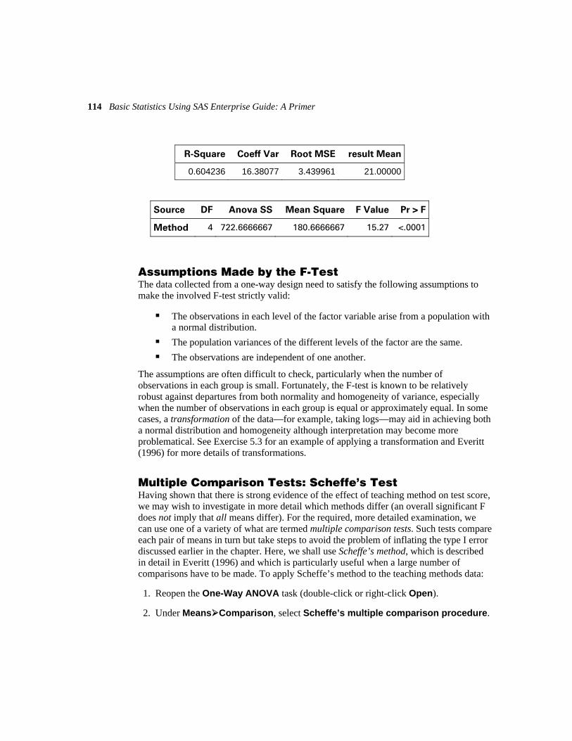
114 Basic Statistics Using SAS Enterprise Guide: A Primer
R-Square Coeff Var Root MSE result Mean
0.604236 16.38077 3.439961 21.00000
Source DF Anova SS Mean Square F Value Pr > F
Method 4 722.6666667 180.6666667 15.27 <.0001
Assumptions Made by the F-Test The data collected from a one-way design need to satisfy the following assumptions to make the involved F-test strictly valid:
The observations in each level of the factor variable arise from a population with a normal distribution.
The population variances of the different levels of the factor are the same.
The observations are independent of one another.
The assumptions are often difficult to check, particularly when the number of observations in each group is small. Fortunately, the F-test is known to be relatively robust against departures from both normality and homogeneity of variance, especially when the number of observations in each group is equal or approximately equal. In some cases, a transformation of the data—for example, taking logs—may aid in achieving both a normal distribution and homogeneity although interpretation may become more problematical. See Exercise 5.3 for an example of applying a transformation and Everitt (1996) for more details of transformations.
Multiple Comparison Tests: Scheffe’s Test Having shown that there is strong evidence of the effect of teaching method on test score, we may wish to investigate in more detail which methods differ (an overall significant F does not imply that all means differ). For the required, more detailed examination, we can use one of a variety of what are termed multiple comparison tests. Such tests compare each pair of means in turn but take steps to avoid the problem of inflating the type I error discussed earlier in the chapter. Here, we shall use Scheffe’s method, which is described in detail in Everitt (1996) and which is particularly useful when a large number of comparisons have to be made. To apply Scheffe’s method to the teaching methods data:
1. Reopen the One-Way ANOVA task (double-click or right-click Open).
2. Under Means Comparison, select Scheffe’s multiple comparison procedure.

Chapter 5: Analysis of Variance 115
3. Click Run.
4. Replace the results of the previous run.
The results are shown in Table 5.4. We see that method 3 differs from methods 1, 2, and 5 but not method 4. Method 5 differs from methods 4 and 3 but not from methods 1 and 2. Methods 4, 1, and 2 do not differ from each other. Essentially, the result from Scheffe’s test produces a grouping of the methods into (3, 4), (4, 1, 2), (2, 5).
Table 5.4 Results from Scheffe’s Multiple Comparison Procedure Applied to the Teaching Methods Data
Alpha 0.05
Error Degrees of Freedom 40
Error Mean Square 11.83333
Critical Value of F 2.60597
Minimum Significant Difference 5.2356
Means with the same letter are not
significantly different.
Scheffe Grouping Mean N method
A 27.444 9 3
A
B A 23.444 9 4
B
B C 19.667 9 1
B C
B C 18.333 9 2
C
C 16.111 9 5

116 Basic Statistics Using SAS Enterprise Guide: A Primer
5.3 Example: Weight Gain in Rats
The data shown in Table 5.5 come from an experiment to study the gain in weight of rats fed on four different diets, distinguished by amount of protein (low and high) and by source of protein (beef and cereal). Ten rats were randomized to each of the four possible diets. The question of interest is how diet affects weight gain.
Table 5.5 Rat Weight Gain for Diets Differing by the Amount of Protein and Source of Protein
Beef Cereal
Low High Low high
90 73 107 98 76 102 95 74
90 118 97 56 64 104 80 111
86 81 98 95 51 107 74 88
72 100 74 82 90 87 67 77
95 117 89 86 78 111 58 92
5.3.1 A First Look at the Rat Weight Gain Data Using Box Plots and Numerical Summaries
For the data on weight gain in rats given in Table 5.5, we first open a new process flow to keep the analyses separate:
1. Select File New Process Flow.
2. To rename the process flow, right-click on the Process Flow tab, select Rename, and type weightgain.

Chapter 5: Analysis of Variance 117
The data are in a SAS data set weight. Add the data set to the process flow:
1. Select File Open Data Local Computer.
2. Browse to the folder containing the SAS data set (c:\saseg\sasdata).
3. Select the file.
4. Click Open.
The data set contains four variables: weightgain, source, level, and diet. The last variable combines information on the source of protein and the level. This can be used to produce a box plot with all four diet types:
1. Select Graph Box Plot.
2. Under Task Roles, assign diet to Horizontal and weightgain to Vertical.
3. Click Run.
The result is shown in Figure 5.2.
Figure 5.2 Box Plots for Weight Gain in Rats Data
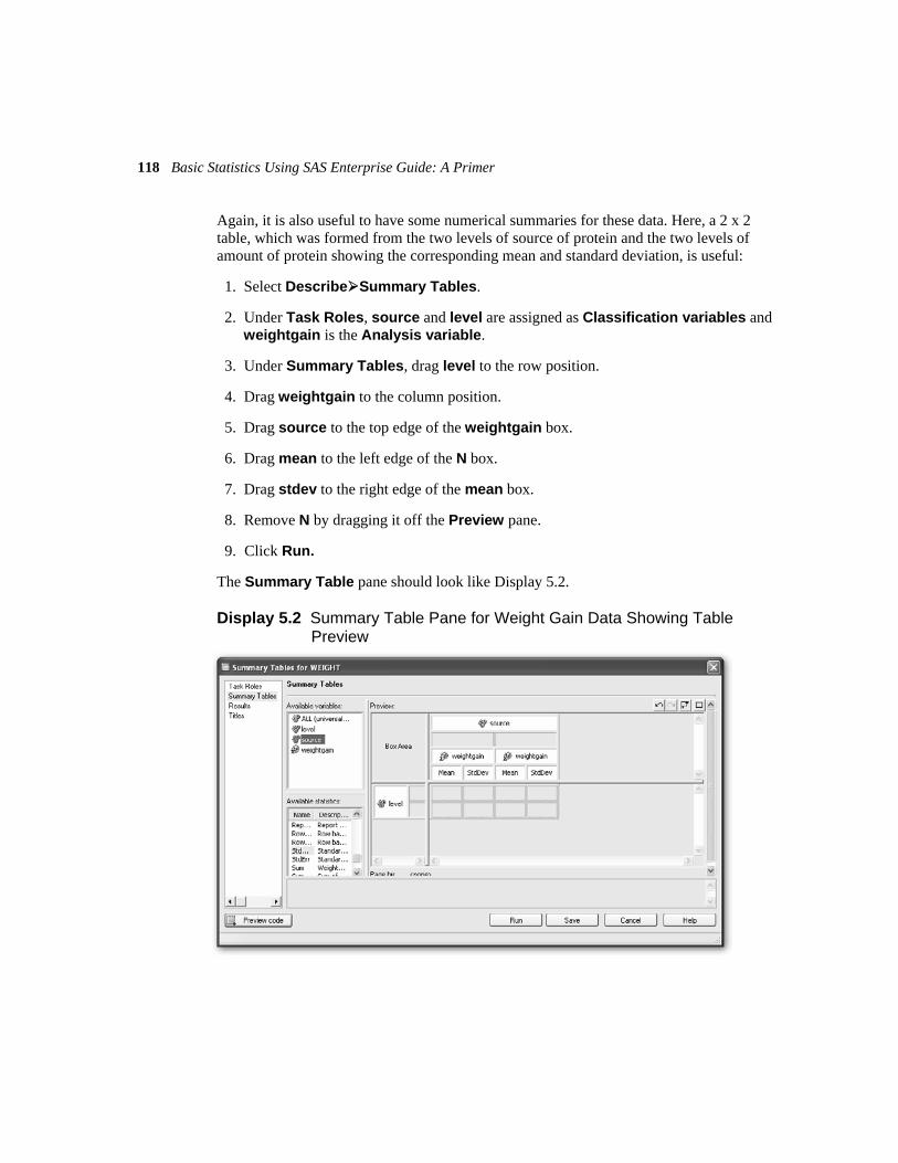
118 Basic Statistics Using SAS Enterprise Guide: A Primer
Again, it is also useful to have some numerical summaries for these data. Here, a 2 x 2 table, which was formed from the two levels of source of protein and the two levels of amount of protein showing the corresponding mean and standard deviation, is useful:
1. Select Describe Summary Tables.
2. Under Task Roles, source and level are assigned as Classification variables and weightgain is the Analysis variable.
3. Under Summary Tables, drag level to the row position.
4. Drag weightgain to the column position.
5. Drag source to the top edge of the weightgain box.
6. Drag mean to the left edge of the N box.
7. Drag stdev to the right edge of the mean box.
8. Remove N by dragging it off the Preview pane.
9. Click Run.
The Summary Table pane should look like Display 5.2.
Display 5.2 Summary Table Pane for Weight Gain Data Showing Table Preview

Chapter 5: Analysis of Variance 119
The results are shown in Table 5.6. The standard deviations in each cell are seen to be very similar to each other, a finding which has implications for the formal analysis of the data (see below). The mean weight gain for beef/high is considerably larger than the other three means, which are quite close to each other.
Table 5.6 Numerical Summary Statistics for Rat Weight Gain Data
source
beef cereal
weightgain weightgain
Crosstabular Summary
Report
Mean StdDev Mean StdDev
level
high 100.00 15.14 85.90 15.02
low 79.20 13.89 83.90 15.71
5.3.2 Weight Gain in Rats: Do Rats Gain More Weight on a Particular Diet?
The data in Table 5.2 are from a simple example of what is known as a factorial design; a factorial design involves the simultaneous study of the effect of two or more factor variables on a response variable of interest. In the rats example, the two factors are source and amount of protein given to the rats. As in the previous example involving different teaching methods, questions of interest about these data concern the equality of weight gain for the two levels of source of protein and for the two levels of amount of protein. So, why not apply a one-way analysis of variance to each factor separately? (In our particular example, there are only two levels, so a one-way analysis of variance is equivalent to the t-test covered in Chapter 2.) The answer to this question is that such an approach would omit an aspect of a factorial design that is often very important, namely testing whether there is an interaction between the two factors. In simple terms, such an effect arises when the effect of applying both factors is either larger (or smaller) than the sum of the effects associated with applying each factor separately. The analysis of variance for a factorial design will include a test for such possible interaction effects. Everitt (1996) includes full details of the analysis of variance for factorial designs.

120 Basic Statistics Using SAS Enterprise Guide: A Primer
To apply the analysis of variance to the rat weight gain data, use the Linear Models task:
1. Select the weight data set.
2. Select Analyze ANOVA Linear Models.
3. Under Task Roles, assign weightgain as the Dependent variable and source and level as Classification variables.
4. Under Model, to set up a factorial model including both main effects and their interaction, select both source and level (CTRL-click on both). The Main, Cross, and Factorial buttons all become active. The Main and Cross buttons could be used to include the main effects and interaction (Cross) in the model separately, but the Factorial button does both. Clicking on the Factorial button results in level, source, and level*source being inserted in the Effects pane.
5. In the Model Options pane, deselect Confidence limits for parameter estimates.
6. Click Run.
The results from running that model are shown in Table 5.7.
Table 5.7 Analysis of Variance Results for the Weight Gain in Rats Data
Class Level Information
Class Levels Values
Level 2 high low
Source 2 beef cereal
Number of Observations Read 40
Number of Observations Used 40
Source DF Sum of Squares Mean Square F Value Pr > F
Model 3 2404.10000 801.36667 3.58 0.0230
Error 36 8049.40000 223.59444
Corrected Total 39 10453.50000

Chapter 5: Analysis of Variance 121
R-Square Coeff Var Root MSE Weightgain Mean
0.229980 17.13819 14.95307 87.25000
Source DF Type I SS Mean Square F Value Pr > F
Level 1 1299.600000 1299.600000 5.81 0.0211
Source 1 220.900000 220.900000 0.99 0.3269
level*source 1 883.600000 883.600000 3.95 0.0545
Source DF Type III SS Mean Square F Value Pr > F
Level 1 1299.600000 1299.600000 5.81 0.0211
Source 1 220.900000 220.900000 0.99 0.3269
level*source 1 883.600000 883.600000 3.95 0.0545
The analysis of variance table in Table 5.7 shows the results of partitioning the variation in the weight gain observations into parts due to amount of protein, to source of protein, and to the interaction of amount and source. The corresponding F-tests show that there is evidence of a difference in weight gain for low and high levels of protein, but no evidence of a difference for source of protein. The F-test for the interaction of the two factors just fails to reach significance at the conventional 5% level, but it may still be of interest to examine in more detail just what such an interaction, if it exists, implies. The test for interaction assesses whether or not the difference between mean weight gain for, say, beef and cereal protein when given at the low level is the same as the corresponding difference when given at the high level. Here, there is some relatively weak evidence that the two differences are not equal. To see more clearly what is happening, we can construct what is sometimes called an interaction plot.

122 Basic Statistics Using SAS Enterprise Guide: A Primer
Interaction Plots The interaction plot is essentially a plot of the four cell means and is an option available within the Linear Models task.
1. Reopen the Linear Models task (double-click or right-click Open).
2. Under Plots Means, select Dependent means for two-way effects and Observed means (Display 5.3).
3. Click Run.
4. Replace the results of the previous run.
Display 5.3 Selecting the Interaction Plot for the Weight Gain in Rats Data
The result is shown in Figure 5.3. The plot suggests that the difference in weight gain for beef and cereal protein is greater when given at the high level than when given at the low level although the effect does not reach the conventional 5% significance level.

Chapter 5: Analysis of Variance 123
Figure 5.3 Interaction Plot for Rat Weight Gain Data
In Table 5.7, there are two analysis of variance tables which are identical except in the labeling of the sums of squares (SS) column where one is labeled Type I SS and the other Type III SS. In the weight gain in rats example where there are an equal number of observations in each cell of the factorial design, the Type I and Type III methods of computing sums of squares give the same results. However, in an unbalanced design where the number of observations in the cells differ, the use of the Type I and Type III of computing sums of squares give different results, as we will illustrate in the next section.
In a factorial design, the assumptions needed for the F-tests in the analysis of variance table to be strictly valid are similar to the assumptions needed for the one-way design listed earlier, namely, normality and homogeneity. The homogeneity assumption at least seems appropriate for the rat weight gain data given that we found in Table 5.6 the standard deviations of the observations in each of the four cells of the design are approximately equal.

124 Basic Statistics Using SAS Enterprise Guide: A Primer
5.4 Example: Mother’s Post-Natal Depression and Child’s IQ
The data shown in Table 5.8 were obtained from an investigation into the effect of mothers’ post-natal depression on child development. Mothers who gave birth to their first-born child in a major teaching hospital in London were divided into two groups, depressed or not depressed, on the basis of their mental state three months after the birth. The children’s fathers were also divided into two groups, namely fathers who had a history of psychiatric illness and fathers who did not. The dependent variable in the study was the child’s IQ at age 4 years. Only girl babies were involved in the study. The question of interest here is how post-natal depression affects a child’s cognitive development.
Table 5.8 Data Obtained in a Study of the Effect of Post-Natal Depression of the Mother on the Child’s Cognitive Development
Mother’s depression Father’s history Child’s IQ at 4 years
1 0 103 1 0 124
1 0 124 1 0 104
1 0 96 2 0 92
1 0 125 1 0 99
1 0 103 1 1 98
1 1 101 1 0 104
2 1 97 2 1 95
1 0 120 2 0 105
1 0 124
(continued)

Chapter 5: Analysis of Variance 125
Table 5.8 (continued)
Mother’s depression Father’s history Child’s IQ at 4 years
1 0 123 1 0 115 1 1 110
1 1 112 1 1 120
1 1 123 2 0 98
1 0 104 2 0 97
1 0 125 1 0 123
1 1 101 2 1 99
1 0 120 2 0 101
1 0 118 1 0 120
1 1 99
Mother’s depression: 1=no, 2=yes. Father’s history: 0=no previous psychiatric history, 1=has a previous psychiatric history.
5.4.1 Summarizing the Post-Natal Depression Data The summary statistics and count of numbers of observations in each cell of the design for the post-natal depression data are obtained in the same way as in the previous examples. Again, we open a new process flow window:
1. Select File New Process Flow.
2. Rename the process flow Post-natal depression (right-click on the Process Flow tab and select Rename).

126 Basic Statistics Using SAS Enterprise Guide: A Primer
The data are in a tab-delimited file, depressionIQ.tab, with the variable names in the first row. To import the data:
1. Select File Import Data Local Computer, browse to the folder c:\saseg\data, select the file and click Open.
2. Under Region to import, check Specify line to use as column headings; line 1 is the default.
3. Under Text format, select Delimited and Tab.
4. Under Column Options, check that the variables have been correctly recognized.
5. Click Run.
For the summary table:
1. Select Describe Summary Tables.
2. Under Task Roles, assign childIQ as the Analysis variable and Mo_depression and Pa_history as the Classification variables.
3. Under Summary Tables, drag Pa_history to the rows position.
4. Drag childIQ to the column heading position.
5. Drag Mo_depression to the top edge of the childIQ box.
6. Drag mean to the left edge of the N box.
7. Drag stdev (std…) to the left edge of the N box. The Summary Tables pane should now look like Display 5.4.
8. Click Run.
The results are shown in Table 5.9.

Chapter 5: Analysis of Variance 127
Display 5.4 Summary Tables Pane for Post-Natal Depression Data
Table 5.9 Numerical Summary Statistics and Cell Counts for IQ Scores from Post-Natal Depression Study
Mo_depression
1 2
ChildIQ ChildIQ
Crosstabular Summary
Report Mean StdDev N Mean StdDev N
Pa_history
0 114.42 10.32 19 98.60 4.83 5
1 108.00 9.77 8 97.00 2.00 3
Table 5.6 suggests that the average IQ is less for children whose mothers suffered from post-natal depression and for children whose father had a previous psychiatric history. Notice also that the numbers of observations in each of the four cells of the table are not the same; the design is said to be unbalanced.

128 Basic Statistics Using SAS Enterprise Guide: A Primer
5.4.2 How Is a Child’s IQ Affected by Post-Natal Depression in the Mother?
The data on post-natal depression and IQ have a very similar structure to the data on weight gain in rats: both data sets involve two factor variables and a response variable. But the numbers of observations in each cell of the post-natal depression data are not equal as they are for the weight gain data. The unequal cell size in the post-natal depression data has serious implications for the data analysis as we will see later.
Finding the analysis of variance table for the IQ scores from the post-natal depression study is straightforward.
1. Select Analyze ANOVA Linear Models.
2. Under Task Roles, assign childIQ as the Dependent variable and Pa_history and Mo_depression, in that order, as the Classification variables.
3. Under Model, to set up a factorial model including both main effects and their interaction, select both Pa_history and Mo_depression (CTRL-click on both), and click on Factorial. The Model pane should look like Display 5.5.
4. Click Run.
The results are shown in Table 5.10.
Display 5.5 Model Pane for Post-Natal Depression Data

Chapter 5: Analysis of Variance 129
Table 5.10 Analysis of Variance Results for the Post-Natal Depression Study
Class Level Information
Class Levels Values
Pa_history 2 0 1
Mo_depression 2 1 2
Number of Observations Read 35
Number of Observations Used 35
Source DF Sum of Squares Mean Square F Value Pr > F
Model 3 1537.768421 512.589474 5.92 0.0026
Error 31 2685.831579 86.639728
Corrected Total 34 4223.600000
R-Square Coeff Var Root MSE ChildIQ Mean
0.364090 8.523852 9.308046 109.2000
Source DF Type I SS Mean Square F Value Pr > F
Pa_history 1 282.975000 282.975000 3.27 0.0804
Mo_depression 1 1222.101866 1222.101866 14.11 0.0007
Pa_histor*Mo_depress 1 32.691555 32.691555 0.38 0.5435
Source DF Type III SS Mean Square F Value Pr > F
Pa_history 1 90.492912 90.492912 1.04 0.3147
Mo_depression 1 1011.820488 1011.820488 11.68 0.0018
Pa_histor*Mo_depress 1 32.691555 32.691555 0.38 0.5435

130 Basic Statistics Using SAS Enterprise Guide: A Primer
In Table 5.10, we see that the Type I and Type III sums of squares for the main effects of a father’s psychiatric history and a mother’s post-natal depression are not the same but they are the same for the interaction term. In a factorial design where there are unequal numbers of observations in each cell of the design, it is no longer possible to partition the variation in the data into non-overlapping or orthogonal sums of squares representing main effects and interactions as it is in a design with equal numbers of observations in each cell. In an unbalanced two-way layout (for example) with factors A and B, there is a proportion of the variance of the response variable that can be attributed to either A or B. The consequence is that A and B together explain less of the variation of the dependent variable than the sum of which each explains alone. The result is that the sum of squares corresponding to a factor depends on which other terms are currently in the model for the observations, so the sums of squares depend on the order in which the factors are considered and represent a comparison of models. For example, for the order A, B, AxB, the sums of squares are such that:
SSA (sum of squares for A): compares model containing only the A main effect with one containing only the overall mean
SSB|A (sum of squares for B given A is already in the model): compares model with both main effects, but no interaction, with one including only the main effect of A
SSAB|A,B (sum of squares for AxB given that A and B are already in the model): compares model including an interaction and main effects with one including only main effects
These are what are called Type I sums of squares. In contrast, Type III sums of squares represent the contribution of each term to a model including all other possible terms. Thus for two-factor designs, the Type III sums of squares represent:
SSA: SSA|B,AB (sum of squares for A given that B and AxB are in the model)
SSB: SSB|A,AB (sum of squares for B given that A and AxB are in the model)
SSAB: SSAB|A,B (sum of squares for AxB given that A and B are in the model)
SAS also has a Type IV sum of squares, which is the same as Type III unless the design contains empty cells.
In a balanced design, Type I and Type III sums of squares are equal; for an unbalanced design they are not equal, and there have been numerous discussions over which type is most appropriate for the analysis of such designs. Authors such as Maxwell and Delaney (1990) and Howell (1992) strongly recommend the use of Type III sums of squares, and they are the default in SAS Enterprise Guide. Nelder (1977) and Aitkin (1978), however, are strongly critical of “correcting” main effects sums of squares for an interaction term involving the corresponding main effect; their criticisms are based on both theoretical and

Chapter 5: Analysis of Variance 131
pragmatic grounds. The arguments are relatively subtle but in essence go something like the following:
When fitting models to data, the principle of parsimony is of critical importance. In choosing among possible models, we do not adopt complex models for which there is no empirical evidence.
So if there is no convincing evidence of an AB interaction, we do not retain the term in the model. Thus, additivity of A and B is assumed unless there is convincing evidence to the contrary.
So the argument proceeds that Type III sum of squares for A in which it is adjusted for AB makes no sense.
First if the interaction term is necessary in the model, then the experimenter will usually wish to consider simple effects of A at each level of B separately. A test of the hypothesis of no A main effect would not usually be carried out if the AB interaction is significant.
If the AB interaction is not significant, then adjusting for it is of no interest and causes a substantial loss of power in testing the A and B main effects.
The issue does not arise so clearly in the balanced case, for there the sum of squares for a main effect is independent of whether interaction is assumed or not. Thus in deciding on possible models for the data, the interaction term is not included unless it has been shown to be necessary, in which case tests on main effects involved in the interaction are not carried out or, if the tests are carried out, no attempt should be made to interpret them.
The arguments of Nelder and Aitkin against the use of Type III sums of squares are powerful and persuasive. Their recommendation to use Type I sums of squares—combined with doing a number of analyses in which main effects are considered in a number of orders—as the most suitable way in which to identify a suitable model for a data set is also convincing and strongly endorsed by the authors of this book.
So for the post-natal depression data, we will now produce another analysis of variance table in which the main effects are considered in the order of mother’s depression followed by father’s psychiatric history, which is the reverse order to what was produced in Table 5.10. To do this:
1. Reopen the Linear Models task (double-click or right-click Open).
2. Under Model, select all the effects and click Remove effects.
3. To reenter the main effects, select Mo_depression and click Main.
4. Repeat with Pa_history.
5. To reenter the interaction, select both effects and click Cross.
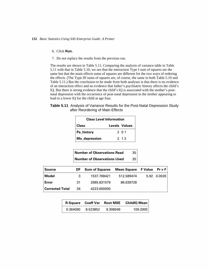
132 Basic Statistics Using SAS Enterprise Guide: A Primer
6. Click Run.
7. Do not replace the results from the previous run.
The results are shown in Table 5.11. Comparing the analysis of variance table in Table 5.11 with that in Table 5.10, we see that the interaction Type I sum of squares are the same but that the main effects sums of squares are different for the two ways of ordering the effects. (The Type III sums of squares are, of course, the same in both Table 5.10 and Table 5.11.) But the conclusion to be made from both analyses is that there is no evidence of an interaction effect and no evidence that father’s psychiatric history affects the child’s IQ. But there is strong evidence that the child’s IQ is associated with the mother’s post-natal depression with the occurrence of post-natal depression in the mother appearing to lead to a lower IQ for the child at age four.
Table 5.11 Analysis of Variance Results for the Post-Natal Depression Study after Reordering of Main Effects
Class Level Information
Class Levels Values
Pa_history 2 0 1
Mo_depression 2 1 2
Number of Observations Read 35
Number of Observations Used 35
Source DF Sum of Squares Mean Square F Value Pr > F
Model 3 1537.768421 512.589474 5.92 0.0026
Error 31 2685.831579 86.639728
Corrected Total 34 4223.600000
R-Square Coeff Var Root MSE ChildIQ Mean
0.364090 8.523852 9.308046 109.2000

Chapter 5: Analysis of Variance 133
Source DF Type I SS Mean Square F Value Pr > FMo_depression 1 1300.859259 1300.859259 15.01 0.0005
Pa_history 1 204.217607 204.217607 2.36 0.1349
Pa_histor*Mo_depress 1 32.691555 32.691555 0.38 0.5435
Source DF Type III SS Mean Square F Value Pr > F
Mo_depression 1 1011.820488 1011.820488 11.68 0.0018
Pa_history 1 90.492912 90.492912 1.04 0.3147
Pa_histor*Mo_depress 1 32.691555 32.691555 0.38 0.5435
5.5 Exercises
Exercise 5.1 The rats data set derives from a study in which the effects of three different poisons and four different treatments on the survival times of rats in hours were of interest. Carry out an appropriate analysis of variance of these data paying particular attention to possible violations of distributional assumptions.
Treatment
Poison A B C D
1 0.31 0.82 0.43 0.45 0.45 1.10 0.45 0.71
0.46 0.88 0.63 0.66 0.43 0.72 0.76 0.62
2 0.36 0.92 0.44 0.56 0.29 0.61 0.35 1.02
0.40 0.49 0.31 0.71 0.23 1.24 0.40 0.38
3 0.22 0.30 0.23 0.30 0.21 0.37 0.25 0.36
0.18 0.38 0.24 0.31 0.23 0.29 0.22 0.22

134 Basic Statistics Using SAS Enterprise Guide: A Primer
Exercise 5.2 The knee data set comes from an investigation described by Kapor (1981) in which the effect of knee-joint angle on the efficiency of cycling was studied. Efficiency was measured in terms of distance (km) pedaled on an ergocycle until exhaustion. The experimenter selected three knee-joint angles of particular interest, 50, 70, and 90 degrees. Ten subjects were randomly allocated to each angle. The drag of the ergocycle was kept constant at 14.7N and subjects were instructed to pedal at a constant speed of 20 km/h until exhaustion.
1. Carry out an initial data analysis to assess whether there are any aspects of the data that might be a cause for concern in later analyses.
2. Calculate the appropriate analysis of variance table for the data.
3. Use a variety of multiple comparison tests to explore differences between the population means for each angle and compare their results.
50 70 90
8.4 10.6 3.27.0 7.5 4.23.0 5.1 3.1
8.0 5.6 6.97.8 10.2 7.2
3.3 11.0 3.54.3 6.8 3.1
3.6 9.4 4.58.0 10.4 3.8
6.8 8.8 3.6

Chapter 5: Analysis of Variance 135
Exercise 5.3 The data in the SAS data set hypertension are from a study described by Maxwell and Delaney (1990) in which the effects of three possible treatments for hypertension were investigated. The details of the treatments are as follows:
Treatment Description Levels
drug medication drug X, drug Y, drug Z biofeed psychological feedback present, absent diet special diet present, absent
All 12 combinations of the three treatments were included in a 3×2×2 design. Seventy-two subjects suffering from hypertension were recruited to the study with six being randomly allocated to each of 12 treatment combinations. Blood pressure measurements were made on each subject after treatment, leading to the data below.
Special diet
Biofeedback Drug No Yes
X
Y
Present
Z
X
Y
Absent
Z
170 175 165 180 160 158
186 194 201 215 219 209
180 187 199 170 204 194
173 194 197 190 176 198
189 194 217 206 199 195
202 228 190 206 224 204
161 173 157 152 181 190
164 166 159 182 187 174
162 184 183 156 180 173
164 190 169 164 176 175
171 173 196 199 180 203
205 199 170 160 179 179
1. Find the analysis of variance table for the data and interpret the results.
2. Construct appropriate graphics as an aid to this interpretation.
3. Re-analyze the data after taking a log transformation and compare the results with those in step 1.
Exercise 5.4 The data in the genotypes data set are from a foster feeding experiment with rat mothers and litters of four different genotypes: A, B, I, and J. The measurement is the litter weight (in grams) after a trial feeding period. Investigate the effect of genotype of mother and litter on litter weight.
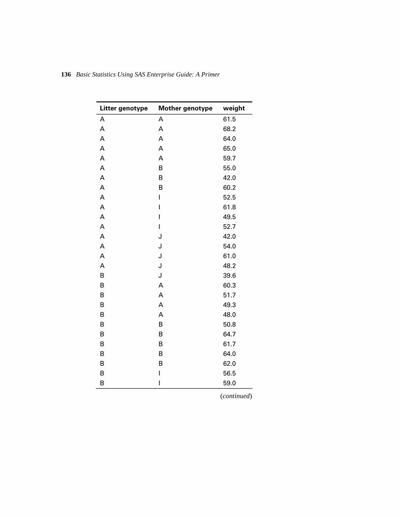
136 Basic Statistics Using SAS Enterprise Guide: A Primer
Litter genotype Mother genotype weight
A A 61.5 A A 68.2 A A 64.0
A A 65.0 A A 59.7
A B 55.0 A B 42.0
A B 60.2 A I 52.5
A I 61.8 A I 49.5
A I 52.7 A J 42.0
A J 54.0 A J 61.0
A J 48.2 B J 39.6
B A 60.3 B A 51.7
B A 49.3 B A 48.0
B B 50.8 B B 64.7
B B 61.7 B B 64.0
B B 62.0 B I 56.5
B I 59.0
(continued)

Chapter 5: Analysis of Variance 137
Exercise 5.4 (continued)
Litter genotype Mother genotype weight
B I 47.2 B I 53.0
B J 51.3 B J 40.5
I A 37.0 I A 36.3
I A 68.0 I B 56.3
I B 69.8 I B 67.0
I I 39.7 I I 46.0
I I 61.3 I I 55.3
I I 55.7 I J 50.0
I J 43.8 I J 54.5
J A 59.0 J A 57.4
J A 54.0 J A 47.0
J B 59.5 J B 52.8
J B 56.0 J I 45.2
(continued)

138 Basic Statistics Using SAS Enterprise Guide: A Primer
Exercise 5.4 (continued)
Litter genotype Mother genotype weight
J I 57.0 J I 61.4
J J 44.8 J J 51.5
J J 53.0 J J 42.0
J J 54.0

C h a p t e r 6
Multiple Linear Regression
6.1 Introduction 140 6.2 Example: Consuming Ice Cream 140
6.2.1 The Ice Cream Data: An Initial Analysis Using Scatterplots 141 6.2.2 Ice Cream Sales: Are They Most Affected by Price or Temperature?
How to Tell Using Multiple Regression 143 6.2.3 Diagnosing the Multiple Regression Model Fitted to the Ice Cream
Consumption Data: The Use of Residuals 146 6.3 Example: Making It Rain by Cloud Seeding 152
6.3.1 The Cloud Seeding Data: Initial Examination of the Data Using
Box Plots and Scatterplots 154 6.3.2 When Is Cloud Seeding Best Carried Out? How to Tell Using Multiple
Regression Models Containing Interaction Terms 158 6.3.3 Diagnosing the Fitted Model for the Cloud Seeding Data Using
Residuals 164 6.4 Exercises 166
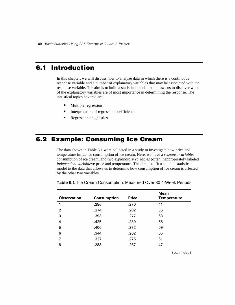
140 Basic Statistics Using SAS Enterprise Guide: A Primer
6.1 Introduction
In this chapter, we will discuss how to analyze data in which there is a continuous response variable and a number of explanatory variables that may be associated with the response variable. The aim is to build a statistical model that allows us to discover which of the explanatory variables are of most importance in determining the response. The statistical topics covered are:
Multiple regression
Interpretation of regression coefficients
Regression diagnostics
6.2 Example: Consuming Ice Cream
The data shown in Table 6.1 were collected in a study to investigate how price and temperature influence consumption of ice cream. Here, we have a response variable: consumption of ice cream, and two explanatory variables (often inappropriately labeled independent variables): price and temperature. The aim is to fit a suitable statistical model to the data that allows us to determine how consumption of ice cream is affected by the other two variables.
Table 6.1 Ice Cream Consumption: Measured Over 30 4-Week Periods
Observation
Consumption
Price Mean
Temperature
1 .386 .270 41 2 .374 .282 56 3 .393 .277 63
4 .425 .280 68 5 .406 .272 69
6 .344 .262 65 7 .327 .275 61
8 .288 .267 47
(continued)

Chapter 6: Multiple Linear Regression 141
Table 6.1 (continued)
Observation
Consumption
Price Mean
Temperature
9 .269 .265 32 10 .256 .277 24 11 .286 .282 28
12 .298 .270 26 13 .329 .272 32
14 .318 .287 40 15 .381 .277 55
16 .381 .287 63 17 .470 .280 72
18 .443 .277 72 19 .386 .277 67
20 .342 .277 60 21 .319 .292 44
22 .307 .287 40 23 .284 .277 32
24 .326 .285 27 25 .309 .282 28
26 .359 .265 33 27 .376 .265 41
28 .416 .265 52 29 .437 .268 64
30 .548 .260 71
6.2.1 The Ice Cream Data: An Initial Analysis Using Scatterplots
The ice cream data in Table 6.1 are in a comma-separated file, icecream.csv, with the names of the variables, also comma-separated, in its first line. The data need to be imported to a SAS data set before they can be analyzed, but files of this type are very straightforward:
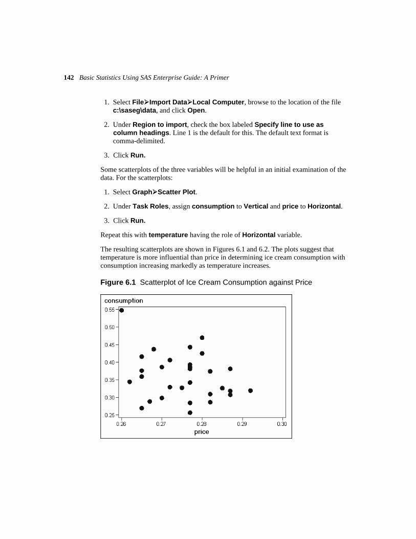
142 Basic Statistics Using SAS Enterprise Guide: A Primer
1. Select File Import Data Local Computer, browse to the location of the file c:\saseg\data, and click Open.
2. Under Region to import, check the box labeled Specify line to use as column headings. Line 1 is the default for this. The default text format is comma-delimited.
3. Click Run.
Some scatterplots of the three variables will be helpful in an initial examination of the data. For the scatterplots:
1. Select Graph Scatter Plot.
2. Under Task Roles, assign consumption to Vertical and price to Horizontal.
3. Click Run.
Repeat this with temperature having the role of Horizontal variable.
The resulting scatterplots are shown in Figures 6.1 and 6.2. The plots suggest that temperature is more influential than price in determining ice cream consumption with consumption increasing markedly as temperature increases.
Figure 6.1 Scatterplot of Ice Cream Consumption against Price
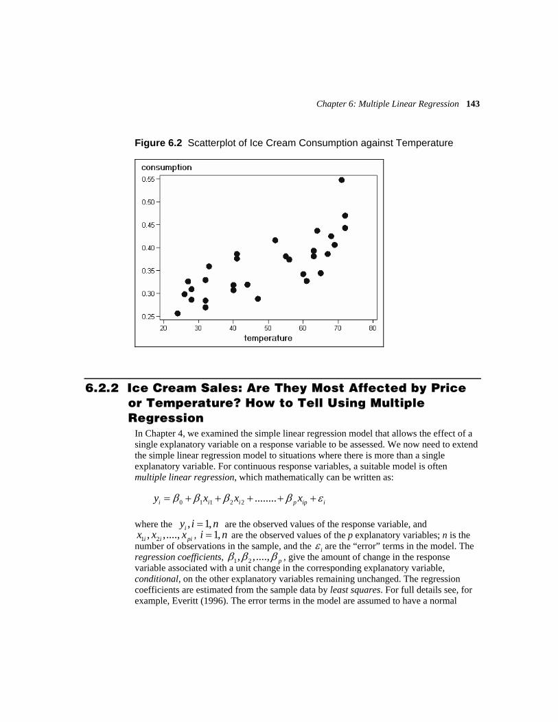
Chapter 6: Multiple Linear Regression 143
Figure 6.2 Scatterplot of Ice Cream Consumption against Temperature
6.2.2 Ice Cream Sales: Are They Most Affected by Price or Temperature? How to Tell Using Multiple Regression
In Chapter 4, we examined the simple linear regression model that allows the effect of a single explanatory variable on a response variable to be assessed. We now need to extend the simple linear regression model to situations where there is more than a single explanatory variable. For continuous response variables, a suitable model is often multiple linear regression, which mathematically can be written as:
0 1 1 2 2 ........i i i p ip iy x x xβ β β β ε= + + + + +
where the , 1,iy i n= are the observed values of the response variable, and
1 2, ,....,i i pix x x , 1,i n= are the observed values of the p explanatory variables; n is the number of observations in the sample, and the iε are the “error” terms in the model. The regression coefficients, 1 2, ,...., pβ β β , give the amount of change in the response variable associated with a unit change in the corresponding explanatory variable, conditional, on the other explanatory variables remaining unchanged. The regression coefficients are estimated from the sample data by least squares. For full details see, for example, Everitt (1996). The error terms in the model are assumed to have a normal

144 Basic Statistics Using SAS Enterprise Guide: A Primer
distribution with mean zero and variance 2σ . The assumed normal distribution for the error terms in the model implies that, for given values of the explanatory variables, the response variable is normally distributed with a mean that is a linear function of the explanatory variables and a variance that is not dependent on the explanatory variables. The variation in the response variable can be partitioned into a part due to regression on the explanatory variables and a residual. The various terms in the partition of the variation of the response variable can be arranged in an analysis of variance table and the F-test of the equality of the regression variance (or mean square) and the residual variance gives a test of the hypothesis that there is no regression on the explanatory variables; i.e., the hypothesis that all the population regression coefficients are zero. Further details are available in Everitt (1996).
We now fit the multiple regression model to the ice cream data. Here, there are two explanatory variables: temperature and price. The multiple regression model is fitted to the data:
1. Select Analyze Regression Linear.
2. Under Task Roles, assign consumption the role of Dependent variable and price and temperature the role of Explanatory variables (Display 6.1). Note that there is no role of Classification variable. The Explanatory variables are all assumed to be quantitative.
3. Click Run.
Display 6.1 Task Roles Pane for Linear Regression of Ice Cream Data

Chapter 6: Multiple Linear Regression 145
The results are shown in Table 6.2. The F-test in the analysis of variance table takes the value 23.27 and has an associated p-value that is very small. Clearly, the hypothesis that both regression coefficients are zero is not tenable. The multiple correlation coefficient gives the correlation between the observed values of the response variable (ice cream consumption) and the values predicted by the fitted model; the square of the coefficient (0.63) gives the proportion of the variance in ice cream consumption accounted for by price and temperature. The negative regression coefficient for price indicates that, for a given mean temperature, consumption decreases with increasing price. But as indicated by the two scatterplots in Section 6.3.1, only the estimated regression coefficient associated with temperature is statistically significant. The regression coefficient of consumption on temperature is estimated to be 0.00303 with an estimated standard error of 0.00047. A one-degree rise in temperature is estimated to increase consumption by 0.00303 units, conditional on price.
Table 6.2 Results from Applying the Multiple Regression Model to the Ice Cream Consumption Data
Number of Observations Read 30
Number of Observations Used 30
Analysis of Variance
Source DF
Sum of
Squares
Mean
Square F Value Pr > F
Model 2 0.07943 0.03972 23.27 <.0001
Error 27 0.04609 0.00171
Corrected Total 29 0.12552
Root MSE 0.04132 R-Square 0.6328
Dependent Mean 0.35943 Adj R-Sq 0.6056
Coeff Var 11.49484

146 Basic Statistics Using SAS Enterprise Guide: A Primer
Parameter Estimates
Variable Label DF
Parameter
Estimate
Standard
Error t Value Pr > |t|
Intercept Intercept 1 0.59655 0.25831 2.31 0.0288
Price Price 1 -1.40176 0.92509 -1.52 0.1413
temperature temperature 1 0.00303 0.00046995 6.45 <.0001
6.2.3 Diagnosing the Multiple Regression Model Fitted to the Ice Cream Consumption Data: The Use of Residuals
An important final stage when fitting a multiple regression model is to investigate whether the assumptions made by the model, such as constant variance and normality of error terms, are reasonable. One way to assess the normality and constant variance assumptions is to look at the residuals from the model-fitting process. In their basic form, residuals are defined as:
Residual=observed response value-fitted response value
Various ways of plotting the residuals can be helpful in assessing particular components of the regression model. The most useful plots are as follows:
A histogram or stem-and-leaf plot of the residuals can be useful checking for symmetry and specifically for the normality of the error terms in the regression model.
Plot the residuals against corresponding values of each explanatory variable. Any sign of a nonlinear relationship in any plot might suggest that a higher order term (e.g., a quadratic) might be necessary for the particular explanatory variable.
Plot the residuals against the fitted values of the response variable (i.e., the values predicted from the model). If the variance of the residuals appears to increase with the fitted values, a transformation of the response may be necessary before refitting the model.
Figure 6.3 shows some idealized residual plots that illustrate each of bullet points above.
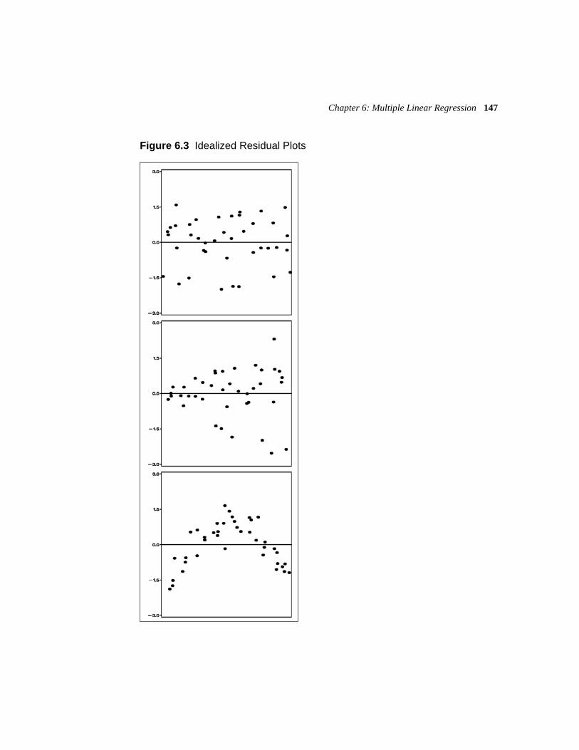
Chapter 6: Multiple Linear Regression 147
Figure 6.3 Idealized Residual Plots

148 Basic Statistics Using SAS Enterprise Guide: A Primer
The simple residuals defined above can be shown to have unequal variances and to be slightly correlated. This correlation makes them less than ideal for detecting problems with fitted models, and the basic residuals are often standardized in some way before being used in a graphical examination of the regression model. Details are given in Rawlings et al. (2001).
To produce plots of residuals from the ice cream data:
1. Reopen the Linear Regression task (double-click or right-click Open).
2. Under Plots Residual, check Standardized vs predicted Y and Standardized vs independents (Display 6.2).
3. Under Predictions, check Original sample in Data to predict and Residuals in Additional statistics (Display 6.3).
4. Click Run.
5. Replace the results of the previous run.
Display 6.2 Selection of Residual Plots for Ice Cream Data

Chapter 6: Multiple Linear Regression 149
Display 6.3 Saving Residuals from Regression of the Ice Cream Data
As well as the residual plots shown in Figure 6.4, a data set is created which contains the predicted values and residuals and which can be used to check the normality of the residuals using the Distribution Analysis task.
1. Select the resulting data set, labeled Linear regression….
2. Select Describe Distribution Analysis.
3. The Task Roles pane (Display 6.4) lists several variables in addition to the original variables: one for the values of consumption predicted by the model and three for different types of residuals. Residual_consumption is the raw residual, i.e., the observed value minus the predicted value; student_consumption is the standardized residual, i.e., the raw residual scaled to have a mean of zero and standard deviation of one. The third, rstudent_consumption, is similar to the standardized residual but with the current observation omitted from the calculations. Assign student_consumption as the Analysis variable.

150 Basic Statistics Using SAS Enterprise Guide: A Primer
4. Under Distributions Normal, check Normal to test for normality.
5. Under Plots, select Histogram Plot.
6. Click Run.
Display 6.4 Task Roles Pane Showing Additional Variables in the Prediction Data Set
The results are given in Figures 6.4 and 6.5. On the whole, the plots all appear satisfactory and give little cause for concern about the assumptions made in fitting the model or for the results obtained for the fitting procedure.
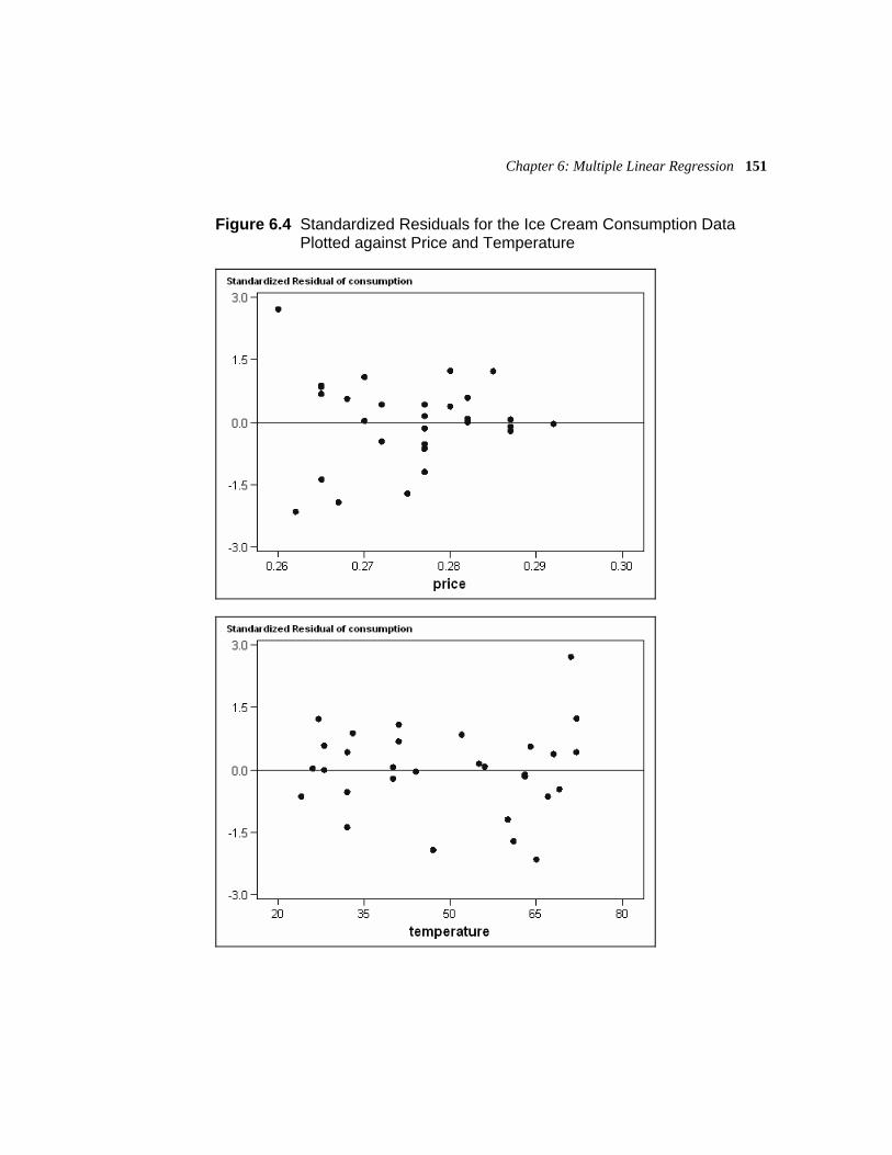
Chapter 6: Multiple Linear Regression 151
Figure 6.4 Standardized Residuals for the Ice Cream Consumption Data Plotted against Price and Temperature
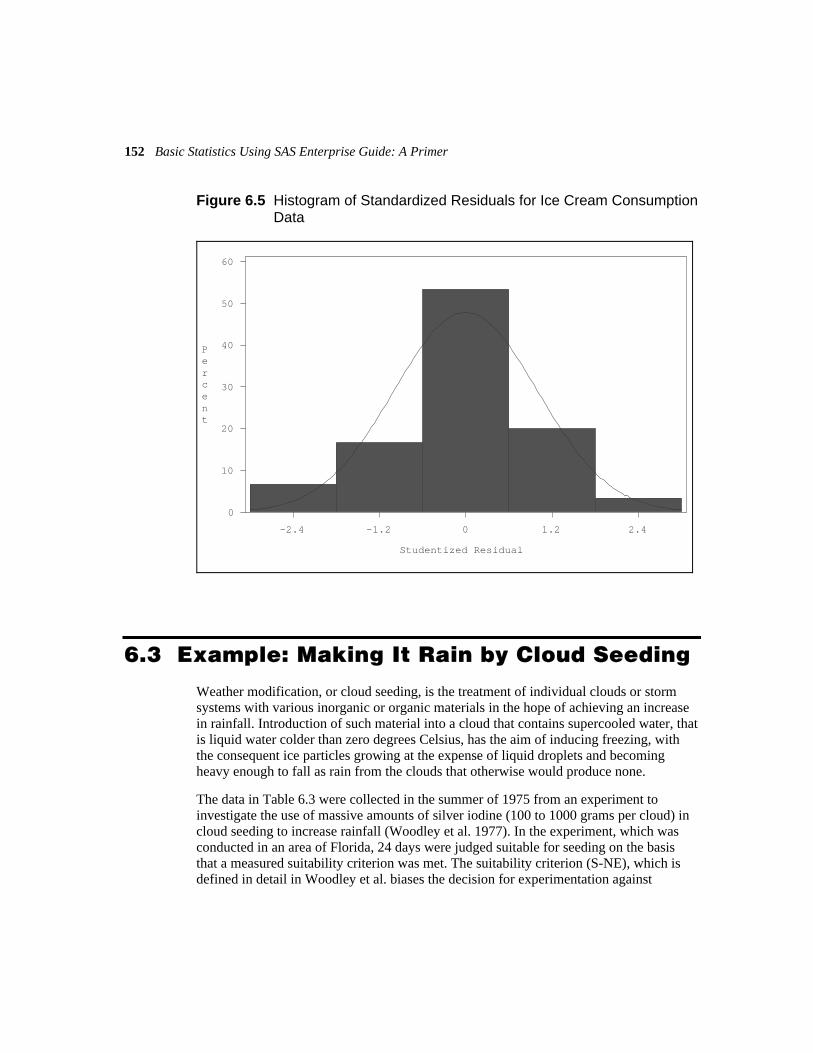
152 Basic Statistics Using SAS Enterprise Guide: A Primer
Figure 6.5 Histogram of Standardized Residuals for Ice Cream Consumption Data
-2.4 -1.2 0 1.2 2.40
10
20
30
40
50
60
Percent
Studentized Residual
6.3 Example: Making It Rain by Cloud Seeding
Weather modification, or cloud seeding, is the treatment of individual clouds or storm systems with various inorganic or organic materials in the hope of achieving an increase in rainfall. Introduction of such material into a cloud that contains supercooled water, that is liquid water colder than zero degrees Celsius, has the aim of inducing freezing, with the consequent ice particles growing at the expense of liquid droplets and becoming heavy enough to fall as rain from the clouds that otherwise would produce none.
The data in Table 6.3 were collected in the summer of 1975 from an experiment to investigate the use of massive amounts of silver iodine (100 to 1000 grams per cloud) in cloud seeding to increase rainfall (Woodley et al. 1977). In the experiment, which was conducted in an area of Florida, 24 days were judged suitable for seeding on the basis that a measured suitability criterion was met. The suitability criterion (S-NE), which is defined in detail in Woodley et al. biases the decision for experimentation against

Chapter 6: Multiple Linear Regression 153
naturally rainy days. On thus defined suitable days, a decision was taken at random as to whether to seed or not. The aim in analyzing the cloud seeding data is to see how rainfall is related to the other variables and, in particular, to determine the effectiveness of seeding.
Table 6.3 Cloud Seeding Data
Seeding Time S-NE Cloudcover Pre-
wetness
Echo
motion
Rainfall
0 0 1.75 13.40 0.274 1 12.85
1 1 2.70 37.90 1.267 0 5.52
1 3 4.10 3.90 0.198 1 6.29
0 4 2.35 5.30 0.526 0 6.11
1 6 4.25 7.10 0.250 0 2.45
0 9 1.60 6.90 0.018 1 3.61
0 18 1.30 4.60 0.307 0 0.47
0 25 3.35 4.90 0.194 0 4.56
0 27 2.85 12.10 0.751 0 6.35
1 28 2.20 5.20 0.084 0 5.06
1 29 4.40 4.10 0.236 0 2.76
1 32 3.10 2.80 0.214 0 4.05
0 33 3.95 6.80 0.796 0 5.74
1 35 2.90 3.00 0.124 0 4.84
1 38 2.05 7.00 0.144 0 11.86
0 39 4.00 11.30 0.398 0 4.45
0 53 3.35 4.20 0.237 1 3.66
1 55 3.70 3.30 0.960 0 4.22
0 56 3.80 2.20 0.230 0 1.16
1 59 3.40 6.50 0.142 1 5.45
1 65 3.15 3.10 0.073 0 2.02
0 68 3.15 2.60 0.136 0 0.82
1 82 4.01 8.30 0.123 0 1.09
0 83 4.65 7.40 0.168 0 0.28

154 Basic Statistics Using SAS Enterprise Guide: A Primer
6.3.1 The Cloud Seeding Data: Initial Examination of the Data Using Box Plots and Scatterplots
For the cloud seeding data, we will construct box plots of the rainfall in each category of the dichotomous explanatory variables (seeding and echomotion) and scatterplots of rainfall against each of the continuous explanatory variables (cloudcover, sne, prewetness, and time). We first create a new process flow for the analysis of these data.
1. Select File New Process Flow.
2. Rename the process flow cloud seeding (right-click on the Process Flow tab and select Rename).
The data are stored in a tab-separated file, cloud.tab, with the variable names in the first line. To import the data:
1. Select File Import Data Local Computer, browse to the location c:\saseg\data, and select and open cloud.tab.
2. Under Region to import, check Specify line to use as column headings. Line 1 is the default.
3. Under Text Format, select Delimited and Tab.
4. Click Run.
For the box plots:
1. Select Graph Box Plot.
2. Assign rainfall to Vertical and seeding to Horizontal.
3. Click Run.
Repeat with echomotion as the horizontal variable.
The plots are shown in Figures 6.6 through 6.11. Both the box plots and the scatterplots show some evidence of two outliers. In particular, the scatterplot of rainfall against cloud cover suggests one very clear outlying observation which on inspection turns out to be the second observation in the data set. For the time being, we shall not remove any observations but simply bear in mind during the modeling process to be described later that outliers may cause difficulties.

Chapter 6: Multiple Linear Regression 155
Figure 6.6 Box Plots of Rainfall for Seeding and Not Seeding Days
Figure 6.7 Box Plots of Rainfall for Moving and Stationary Echomotion

156 Basic Statistics Using SAS Enterprise Guide: A Primer
Figure 6.8 Scatterplot of Rainfall against Time
Figure 6.9 Scatterplot of Rainfall against S-NE Criterion

Chapter 6: Multiple Linear Regression 157
Figure 6.10 Scatterplot of Rainfall against Cloud Cover
Figure 6.11 Scatterplot of Rainfall against Prewetness

158 Basic Statistics Using SAS Enterprise Guide: A Primer
6.3.2 When Is Cloud Seeding Best Carried Out? How to Tell Using Multiple Regression Models Containing Interaction Terms
For the cloud seeding data, one thing to note about the explanatory variables is that two of them, seeding and echomotion, are binary variables. Should such an explanatory variable be allowed in a multiple regression model? In fact, there is really no problem in including such variables in the model since, in a strict sense, the explanatory variables are assumed to be fixed rather than random. In practice, of course, fixed explanatory variables are rarely the case and so the results from a multiple regression analysis are interpreted as being conditional on the observed values of the explanatory variables; this rather arcane point is discussed in more detail in Everitt (1996). It is only the response variable that is considered to be random.
In the cloud seeding example, there are theoretical reasons to consider a particular model for the data (Woodley et al. 1977), namely one in which the effect of some of the other explanatory variables is modified by seeding. So, the model we will consider is one that allows interaction terms for seeding with each of the other explanatory variables except time.
For the analysis of the ice cream data in the previous section, we used the linear regression task (Analyze Regression Linear) to do the analysis. It is also possible to do multiple regression using the Linear Models task (Analyze ANOVA Linear Models) introduced in Chapter 5. The choice between them is largely a matter of which is more convenient for the particular analysis as they offer somewhat different features. The Linear Models task can accommodate both categorical (with more than two categories) and continuous predictors and interactions can be specified in the model.
The Linear Regression task can accommodate only continuous predictors and binary variables. For categorical variables with more than two categories, dummy variables would need to be derived beforehand (Everitt, 1996, and Chapter 7 of this book). To enter an interaction term between two variables in Linear Regression, a new variable needs to be calculated as the product of the two variables, and this new variable needs to be entered into the model. An advantage of the Linear Regression task is that it offers a number of variable selection methods, whereas Linear Models does not. For details of variable selection methods see Everitt (1996).
Since the model to be fitted to the cloud seeding data requires a number of interactions, the Linear Models task will be more convenient and this will therefore be used.
1. Select Analyze ANOVA Linear Models.
2. Under Task Roles, rainfall is the Dependent variable, and the remaining variables are treated as Quantitative variables.

Chapter 6: Multiple Linear Regression 159
3. Under Model, select all the variables, and click Main to enter their main effects.
4. To enter the required interactions with seeding, first click on seeding, then CTRL- click on the other variable in the interaction, and then click the Cross button. Repeat this for each interaction with seeding. When all the terms have been entered, the Model panel should look like Display 6.5.
5. Click Run.
Display 6.5 Model Panel for Cloud Seeding Data
The results of fitting the specified model are shown in Table 6.4. The first thing to note about Table 6.4 is the presence of both Type I and Type III sums of squares. As we would expect from our discussion of both types of sums of squares in the previous chapter, they lead to different p-values for assessing the statistical significance of the estimated regression coefficients. We should also note that the p-values for the Type III sums of squares are identical to the p-values given for each estimated regression coefficient found from a t-test of the hypothesis that the corresponding population coefficient is zero (the t-statistic is simply the regression coefficient estimate divided by its estimated standard error). The p-values are identical because the regression coefficients are estimated conditional on all other terms in the model, and the Type III sums of squares are essentially found in the same way. Here, where we are primarily interested in the interaction effects of other explanatory variables with seeding, it is appropriate to use the Type III sums of squares or equivalently the t-tests on each coefficient to judge which interactions are of most importance. But if we wanted to assess

160 Basic Statistics Using SAS Enterprise Guide: A Primer
the main effects in the model, then Type III sums of squares would not be the ones to use as argued in Chapter 5.
Table 6.4 Results of Fitting a Multiple Regression Model with Interactions to the Cloud Seeding Data
Source DF Sum of Squares Mean Square F Value Pr > F
Model 10 159.1460026 15.9146003 3.27 0.0243
Error 13 63.1888933 4.8606841
Corrected Total 23 222.3348958
R-Square Coeff Var Root MSE rainfall Mean
0.715794 50.07353 2.204696 4.402917
Source DF Type I SS Mean Square F Value Pr > F
Seeding 1 1.28343750 1.28343750 0.26 0.6160
Time 1 55.31045354 55.31045354 11.38 0.0050
Sne 1 11.49594672 11.49594672 2.37 0.1481
Cloudcover 1 2.00314031 2.00314031 0.41 0.5321
Prewetness 1 0.33184258 0.33184258 0.07 0.7980
Echomotion 1 15.15890800 15.15890800 3.12 0.1009
seeding*sne 1 33.15823806 33.15823806 6.82 0.0215
seeding*cloudcover 1 38.82083001 38.82083001 7.99 0.0143
seeding*prewetness 1 1.36347743 1.36347743 0.28 0.6053
seeding*echomotion 1 0.21972842 0.21972842 0.05 0.8349

Chapter 6: Multiple Linear Regression 161
Source DF Type III SS Mean Square F Value Pr > F
Seeding 1 60.47295296 60.47295296 12.44 0.0037
Time 1 15.66429701 15.66429701 3.22 0.0959
Sne 1 1.20110501 1.20110501 0.25 0.6274
Cloudcover 1 15.40695933 15.40695933 3.17 0.0984
Prewetness 1 6.32677854 6.32677854 1.30 0.2745
Echomotion 1 12.93729038 12.93729038 2.66 0.1268
seeding*sne 1 30.94793564 30.94793564 6.37 0.0254
seeding*cloudcover 1 19.77764964 19.77764964 4.07 0.0648
seeding*prewetness 1 1.58289424 1.58289424 0.33 0.5780
seeding*echomotion 1 0.21972842 0.21972842 0.05 0.8349
Parameter Estimate Standard Error t Value Pr > |t|
Intercept -0.34624093 2.78773403 -0.12 0.9031
Seeding 15.68293481 4.44626606 3.53 0.0037
Time -0.04497427 0.02505286 -1.80 0.0959
Sne 0.41981393 0.84452994 0.50 0.6274
Cloudcover 0.38786207 0.21785501 1.78 0.0984
Prewetness 4.10834188 3.60100694 1.14 0.2745
Echomotion 3.15281358 1.93252592 1.63 0.1268
seeding*sne -3.19719006 1.26707204 -2.52 0.0254
seeding*cloudcover -0.48625492 0.24106012 -2.02 0.0648
seeding*prewetness -2.55706696 4.48089584 -0.57 0.5780
seeding*echomotion -0.56221845 2.64429975 -0.21 0.8349

162 Basic Statistics Using SAS Enterprise Guide: A Primer
The tests of the interactions in the model suggest that the interaction of seeding with the S-NE criterion significantly affects rainfall. A suitable graph will help in the interpretation of the significant seeding x S-NE criterion interaction. For this graph, we can use the Line Plot task to show the relationship between rainfall and suitability for seeding (S-NE) on days on which seeding did and did not occur.
1. Select Graph Line Plot.
2. Under Line Plot, select Multiple line plots by group column as the type of plot.
3. Under Task Roles, assign rainfall to Vertical, sne to Horizontal, and seeding to Group charts by.
4. Under Appearance Plots, decide how the data for seeding and non-seeding days are distinguished in the plot. The default is to use different colors with the same line type and plotting symbol. Here, we will illustrate the use of different line types and plotting symbols. The panel in the center of the pane shows the two values of seeding, 0 and 1. Highlighting either of these (by clicking on it) shows how the line and data points will be plotted for that group of observations. A solid line is the default and a circle as the plotting symbol. Leaving the values for seeding=0 at their defaults, we change the values for seeding=1 to a dashed line and triangle as the plotting symbol (see Display 6.6).
5. Under Interpolations, select regression for both subgroups (seeding: 0 and 1) which will fit and draw a separate regression line for each group.
6. Click Run.
The result is shown in Figure 6.12.
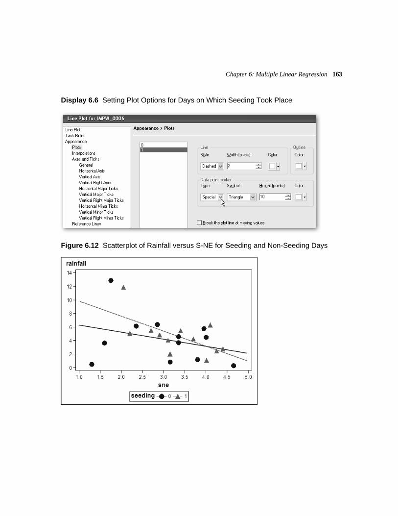
Chapter 6: Multiple Linear Regression 163
Display 6.6 Setting Plot Options for Days on Which Seeding Took Place
Figure 6.12 Scatterplot of Rainfall versus S-NE for Seeding and Non-Seeding Days

164 Basic Statistics Using SAS Enterprise Guide: A Primer
The plot suggests that for smaller S-NE values, seeding produces greater rainfall than no seeding, whereas seeding tends to produce less rainfall for larger S-NE values. The crossover point is at an S-NE value of approximately 4 which might suggest that, for most success, seeding should be applied when the S-NE criterion is less than 4.
6.3.3 Diagnosing the Fitted Model for the Cloud Seeding Data Using Residuals
For the cloud seeding data, we will plot residuals against predicted value and produce a probability plot of residuals to examine their normality.
The process is very similar to that for the ice cream data, even though a different task has been used for the analysis.
1. Reopen the Linear Models task (double-click or right-click Open).
2. Under Plots Residual, check Standardized vs. predicted Y.
3. Under Predictions, check Original data as the Data to predict and Residuals as Additional statistics.
4. Click Run.
5. Replace the results of the previous run.
A new data set is created containing the predicted values and residuals as well as the original variables, and this new data set is used to check the normality of the residuals.
1. Make the new data set active (by clicking on it).
2. Select Describe Distribution Analysis.
3. Under Task Roles, student_rainfall is the Analysis variable.
4. Under Distributions Normal, check Normal (we also changed the line color to black here).
5. Under Plots, select Probability Plot.
6. Click Run.

Chapter 6: Multiple Linear Regression 165
The results are shown in Figures 6.13 and 6.14. The plot of residuals against fitted values suggest that two observations (numbers 1 and 15) are outliers, and it may be of interest to refit the model with the outliers removed (see Exercise 6.2). The normal probability plot shows little evidence of any worrying departure from normality.
Figure 6.13 Plot of Standardized Residuals versus Fitted Rainfall for the Model Fitted to the Cloud Seeding Data
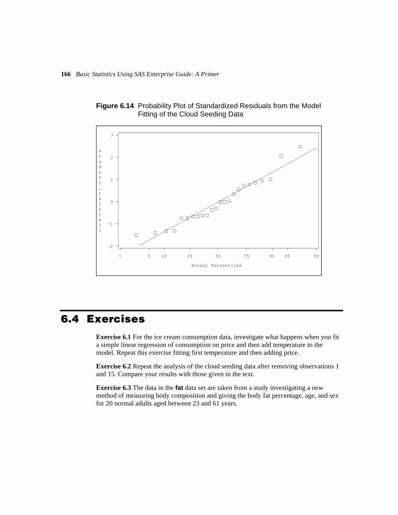
166 Basic Statistics Using SAS Enterprise Guide: A Primer
Figure 6.14 Probability Plot of Standardized Residuals from the Model Fitting of the Cloud Seeding Data
1 5 10 25 50 75 90 95 99
-2
-1
0
1
2
3
student_rainfall
Normal Percentiles
6.4 Exercises
Exercise 6.1 For the ice cream consumption data, investigate what happens when you fit a simple linear regression of consumption on price and then add temperature to the model. Repeat this exercise fitting first temperature and then adding price.
Exercise 6.2 Repeat the analysis of the cloud seeding data after removing observations 1 and 15. Compare your results with those given in the text.
Exercise 6.3 The data in the fat data set are taken from a study investigating a new method of measuring body composition and giving the body fat percentage, age, and sex for 20 normal adults aged between 23 and 61 years.

Chapter 6: Multiple Linear Regression 167
1. Construct a scatterplot percentage fat against age labeling the points according to sex.
2. Fit a multiple regression model to the data using Fat as the response variable and Age and Sex as explanatory variables. Interpret the results with the help of a scatterplot showing the essential features of the fitted model.
3. Fit a further model which allows an interaction between Age and Sex and again construct a diagram that will help you interpret the results.
Age Sex % Fat
23 M 9.523 F 27.927 M 7.8
27 M 17.839 F 31.4
41 F 25.945 M 27.4
49 F 25.250 F 31.1
53 F 34.753 F 42.0
54 F 29.156 F 32.5
57 F 30.358 F 33.0
58 F 33.860 F 41.1
61 F 34.5
Exercise 6.4 The data in the Microsoft Office Excel spreadsheet usair.xls, mentioned in Chapter 1, relate to air pollution in 41 U.S. cities. Seven variables are recorded for each of the cities:
• SO2 content of air in micrograms per cubic meter
• Average annual temperature in °F
• Number of manufacturing enterprises employing 20 or more workers

168 Basic Statistics Using SAS Enterprise Guide: A Primer
• Population size (1970 census) in thousands
• Average annual wind speed in miles per hour
• Average annual precipitation in inches
• Average number of days with precipitation per year
so
2 temperature factories population wind rain rainydays
10 70.3 213 582 6 7.05 3613 61 91 132 8.2 48.52 10012 56.7 453 716 8.7 20.66 67
17 51.9 454 515 9 12.95 8656 49.1 412 158 9 43.37 127
36 54 80 80 9 40.25 11429 57.3 434 757 9.3 38.89 111
14 68.4 136 529 8.8 54.47 11610 75.5 207 335 9 59.8 128
24 61.5 368 497 9.1 48.34 115110 50.6 3344 3369 10.4 34.44 122
28 52.3 361 746 9.7 38.74 12117 49 104 201 11.2 30.85 103
8 56.6 125 277 12.7 30.58 8230 55.6 291 593 8.3 43.11 123
9 68.3 204 361 8.4 56.77 11347 55 625 905 9.6 41.31 111
35 49.9 1064 1513 10.1 30.96 12929 43.5 699 744 10.6 25.94 137
14 54.5 381 507 10 37 9956 55.9 775 622 9.5 35.89 105
14 51.5 181 347 10.9 30.18 9811 56.8 46 244 8.9 7.77 58
46 47.6 44 116 8.8 33.36 13511 47.1 391 463 12.4 36.11 166
23 54 462 453 7.1 39.04 132
(continued)

Chapter 6: Multiple Linear Regression 169
so
2 temperature factories population wind rain rainydays
65 49.7 1007 751 10.9 34.99 155 26 51.5 266 540 8.6 37.01 134 69 54.6 1692 1950 9.6 39.93 115
61 50.4 347 520 9.4 36.22 147 94 50 343 179 10.6 42.75 125
10 61.6 337 624 9.2 49.1 105 18 59.4 275 448 7.9 46 119
9 66.2 641 844 10.9 35.94 78 10 68.9 721 1233 10.8 48.19 103
28 51 137 176 8.7 15.17 89 31 59.3 96 308 10.6 44.68 116
26 57.8 197 299 7.6 42.59 115 29 51.1 379 531 9.4 38.79 164
31 55.2 35 71 6.5 40.75 148 16 45.7 569 717 11.8 29.07 123
Use multiple regression to investigate which of the other variables most determine pollution as indicated by the SO
2 content of the air. (Preliminary investigation of the data
may be necessary to identify possible outliers and pairs of explanatory variables that are so highly correlated that they may cause problems for model fitting.)

170 Basic Statistics Using SAS Enterprise Guide: A Primer

C h a p t e r 7
Logistic Regression
7.1 Introduction 172 7.2 Example: Myocardial Infarctions 172
7.2.1 Myocardial Infarctions: What Predicts a Past History of Myocardial
Infarctions? Answering the Question Using Logistic Regression 174
7.2.2 Odds 173 7.2.3 Applying the Logistic Regression Model with a Single Explanatory
Variable 173 7.2.4 Interpreting the Regression Coefficient in the Fitted Logistic Regression
Model 173 7.2.5 Applying the Logistic Regression Model Using
SAS Enterprise Guide 173 7.3 Exercises 173

172 Basic Statistics Using SAS Enterprise Guide: A Primer
7.1 Introduction
In this chapter, we will describe how to deal with data where there are a binary response variable and a number of explanatory variables. The aim is to see how the explanatory variables affect the response variable. The statistical topics to be covered are:
Regression model for a binary response variable: Logistic regression
What the logistic regression model tells us: Interpretation of regression coefficients and odds ratios
7.2 Example: Myocardial Infarctions
The data in Table 7.1 come from a study described in Kasser and Bruce (1969). A total of 117 male coronary patients were studied to try to determine how history of past myocardial infarctions is dependent on the other variables observed.
Table 7.1 Data on History of Past Myocardial Infarctions
42 2 1 1 0 50 0 0 1 0 35 2 1 1 0 55 3 1 1 1 66 2 1 1 0 72 3 0 1 1 34 2 1 1 0 51 1 0 1 0 56 2 1 1 0 56 3 1 1 0 68 3 1 1 0 46 1 1 1 0
55 2 1 1 0 56 3 1 1 0 49 3 0 1 0 69 1 0 1 0 41 2 1 1 0 63 2 1 1 0 55 2 0 1 1 51 3 1 1 1
62 0 1 0 1 53 1 1 1 0 58 0 1 1 0 49 1 0 1 1 46 2 1 1 1 53 0 1 0 0 43 2 1 1 0 58 3 1 1 0
44 2 0 1 1 57 3 0 1 0 39 2 0 1 0 38 3 1 1 0 50 1 0 1 0 57 1 0 1 1 66 3 0 1 1 50 1 1 0 0
73 3 0 1 0 62 2 1 1 0 50 2 1 1 0 38 1 1 1 0 48 2 1 1 0 73 2 0 1 0 45 3 0 1 0 58 1 1 0 0
53 2 1 1 0 44 2 0 1 0 53 0 0 1 0 69 0 0 1 0 51 3 1 1 1 63 3 1 1 0 56 3 1 1 1 66 0 0 1 0
51 3 1 1 1 59 1 0 1 0 49 2 1 1 1 49 2 0 1 0
(continued)
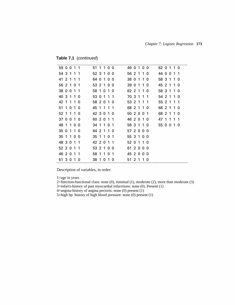
Chapter 7: Logistic Regression 173
Table 7.1 (continued)
59 0 0 1 1 51 1 1 0 0 49 0 1 0 0 62 0 1 1 0
54 3 1 1 1 52 3 1 0 0 56 2 1 1 0 44 0 0 1 1 41 2 1 1 1 64 0 1 0 0 38 0 1 1 0 58 3 1 1 0
56 2 1 0 1 53 2 1 0 0 39 0 1 1 0 45 2 1 1 0 38 0 0 1 1 58 1 0 1 0 62 2 1 1 0 58 3 1 1 0
40 3 1 1 0 42 1 1 1 0
53 0 1 1 1 58 2 0 1 0
70 3 1 1 1 53 2 1 1 1
54 2 1 1 0 55 2 1 1 1
51 1 0 1 0 45 1 1 1 1 68 2 1 1 0 68 2 1 1 0 52 1 1 1 0 42 3 0 1 0 50 2 0 0 1 68 2 1 1 0
37 0 0 1 0 60 2 0 1 1 46 2 0 1 0 47 1 1 1 1 48 1 1 0 0 34 1 1 0 1 58 3 1 1 0 55 0 0 1 0
35 0 1 1 0 64 2 1 1 0 57 2 0 0 0 35 1 1 0 0 35 1 1 0 1 55 3 1 0 0
48 3 0 1 1 42 2 0 1 1 52 0 1 1 0 52 2 0 1 1 53 2 1 0 0 61 2 0 0 0
46 2 0 1 1 58 1 1 0 1 45 2 0 0 0 51 3 0 1 0 38 1 0 1 0 51 2 1 1 0
Description of variables, in order:
1=age in years 2=function-functional class: none (0), minimal (1), moderate (2), more than moderate (3) 3=infarct-history of past myocardial infarctions: none (0). Present (1) 4=angina-history of angina pectoris: none (0) present (1) 5=high bp: history of high blood pressure: none (0) present (1)
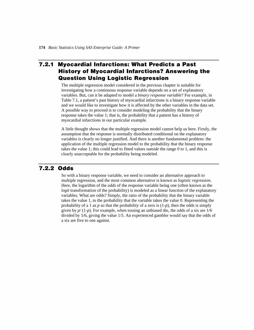
174 Basic Statistics Using SAS Enterprise Guide: A Primer
7.2.1 Myocardial Infarctions: What Predicts a Past History of Myocardial Infarctions? Answering the Question Using Logistic Regression
The multiple regression model considered in the previous chapter is suitable for investigating how a continuous response variable depends on a set of explanatory variables. But, can it be adapted to model a binary response variable? For example, in Table 7.1, a patient’s past history of myocardial infarctions is a binary response variable and we would like to investigate how it is affected by the other variables in the data set. A possible way to proceed is to consider modeling the probability that the binary response takes the value 1; that is, the probability that a patient has a history of myocardial infarctions in our particular example.
A little thought shows that the multiple regression model cannot help us here. Firstly, the assumption that the response is normally distributed conditional on the explanatory variables is clearly no longer justified. And there is another fundamental problem: the application of the multiple regression model to the probability that the binary response takes the value 1; this could lead to fitted values outside the range 0 to 1, and this is clearly unacceptable for the probability being modeled.
7.2.2 Odds So with a binary response variable, we need to consider an alternative approach to multiple regression, and the most common alternative is known as logistic regression. Here, the logarithm of the odds of the response variable being one (often known as the logit transformation of the probability) is modeled as a linear function of the explanatory variables. What are odds? Simply, the ratio of the probability that the binary variable takes the value 1, to the probability that the variable takes the value 0. Representing the probability of a 1 as p so that the probability of a zero is (1-p), then the odds is simply given by p/ (1-p). For example, when tossing an unbiased die, the odds of a six are 1/6 divided by 5/6, giving the value 1/5. An experienced gambler would say that the odds of a six are five to one against.

Chapter 7: Logistic Regression 175
But back to the logistic regression model which in mathematical terms can be written as:
0 1 1 2 2log( ) .....1 p p
p x x xp
β β β β= + + +−
where 1 2, ,....., px x x are the explanatory variables. Now as p varies between 0 and 1, the logit transformation of p varies between minus and plus infinity, thus removing directly one of the problems mentioned above. The model can be rewritten in terms of the probability p as:
0 1 1 2 2
0 1 1 2 2
exp( .... )1 exp( .... )
p p
p p
x x xp
x x xβ β β ββ β β β+ + +
=+ + + +
Full details of the distributional assumptions of the model and of how the parameters in the model are estimated are given in Der and Everitt (2005). Below however, we will concentrate on how to obtain estimates of the parameters, 0 1 2, , ,....., pβ β β β using SAS Enterprise Guide and on how to interpret the estimates after we find them.
7.2.3 Applying the Logistic Regression Model with a Single Explanatory Variable
We shall apply the logistic regression model to the data in Table 7.1, first using only the single explanatory variable, angina; considering this simple model will serve to clarify some of the points raised above. The data are in a comma-separated file, coronary.csv, with the variable names in the first line. To read them into a SAS data set:
1. Select File Import Data Local Computer, navigate to c:\saseg\data, select it and click Open.
2. Under Region to import, check the box labeled Specify line to use as column headings. Line 1 is the default. Under Text Format, the default is Delimited and so it does not need to be changed.
3. Under Column Options, check that the variables have been correctly assigned.
4. Click Run.

176 Basic Statistics Using SAS Enterprise Guide: A Primer
For the logistic model:
1. Select Analyze Regression Logistic.
2. Under Task Roles, assign mi the role of Dependent variable. With mi highlighted, alter the Response variable sort order from Ascending to Descending by clicking on Sort order and use the drop-down menu (Display 7.1). By default, the lower value is treated as the response to be modeled; altering the sort order reverses this. Assign angina the role of Quantitative variables.
3. Under Model, select angina, and click Main to enter its main effect into the model.
4. Click Run.
The results are shown in Table 7.2.
Display 7.1 Task Roles Pane for Logistic Regression: Altering the Response Variable Sort Order
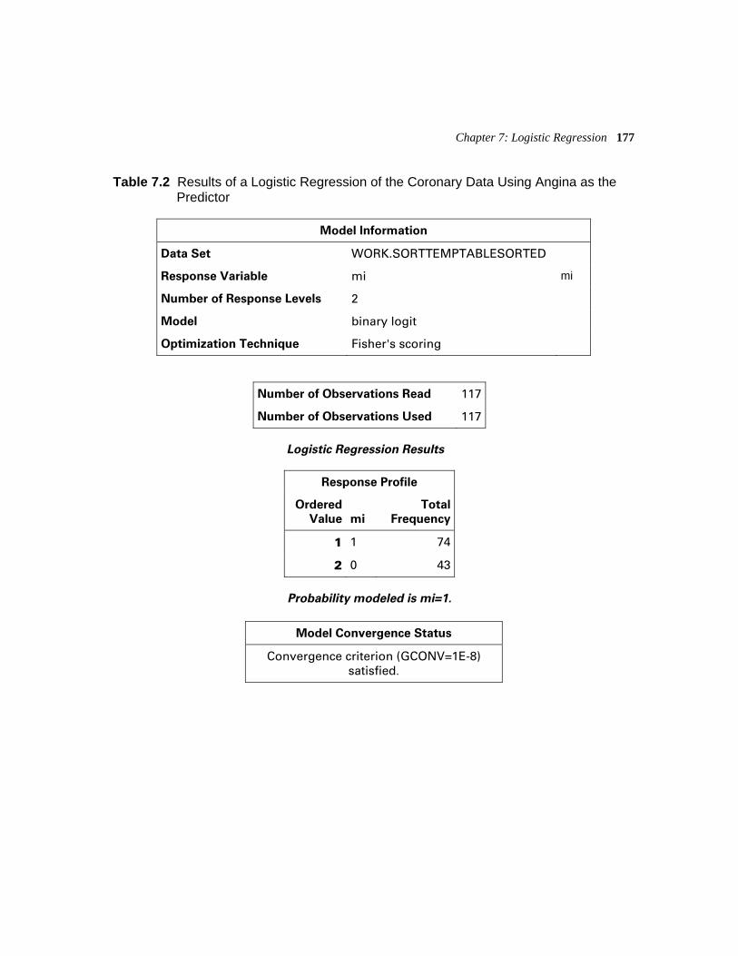
Chapter 7: Logistic Regression 177
Table 7.2 Results of a Logistic Regression of the Coronary Data Using Angina as the Predictor
Model Information
Data Set WORK.SORTTEMPTABLESORTED
Response Variable mi mi
Number of Response Levels 2
Model binary logit
Optimization Technique Fisher's scoring
Number of Observations Read 117
Number of Observations Used 117
Logistic Regression Results
Response Profile
Ordered
Value mi
Total
Frequency
1 1 74
2 0 43
Probability modeled is mi=1.
Model Convergence Status
Convergence criterion (GCONV=1E-8) satisfied.

178 Basic Statistics Using SAS Enterprise Guide: A Primer
Model Fit Statistics
Criterion
Intercept
Only
Intercept
and
Covariates
AIC 155.884 154.140
SC 158.646 159.664
-2 Log L 153.884 150.140
Testing Global Null Hypothesis: BETA=0
Test Chi-Square DF Pr > ChiSq
Likelihood Ratio 3.7443 1 0.0530
Score 3.4512 1 0.0632
Wald 3.2368 1 0.0720
Analysis of Maximum Likelihood Estimates
Parameter DF Estimate
Standard
Error
Wald
Chi-Square Pr > ChiSq
Intercept 1 1.4469 0.5557 6.7791 0.0092
Angina 1 -1.0674 0.5933 3.2368 0.0720
Logistic Regression Results
Odds Ratio Estimates
Effect
Point
Estimate
95% Wald
Confidence Limits
Angina 0.344 0.107 1.100

Chapter 7: Logistic Regression 179
Association of Predicted Probabilities and
Observed Responses
Percent Concordant 20.8 Somers' D 0.137
Percent Discordant 7.2 Gamma 0.488
Percent Tied 72.0 Tau-a 0.064
Pairs 3182 C 0.568
7.2.4 Interpreting the Regression Coefficient in the Fitted Logistic Regression Model
For now, we will concentrate on how to interpret the estimated regression coefficient for angina (shown under Analysis of Maximum Likelihood Estimates in Table 7.2). The fitted model is:
log(odds of a past infarct)=1.447–1.067angina
So for patients with no past history of angina, that is angina=0, we have:
log(odds of a past infarct)=1.447
and for patients with a past history of angina, that is angina=1:
log(odds of a past infarct)=1.447–1.067
Taking the difference of the two log odds we have:
log(odds of an infarct for patients with angina)–log(odds of an infarct for patients without angina)=log(odds for patients with angina/odds for patients without angina)=-1.067
We can now see that for a dichotomous explanatory variable coded zero/one, the estimated regression coefficient is simply the log of the odds ratio. Rather than dealing with the log, we can find the odds ratio itself simply by exponentiating the regression coefficient. The odds ratio is conveniently provided in Table 7.2 in the Odds Ratio Estimates section of the table; in the Point Estimate column, the odds ratio is seen to take the value of 0.344.
How is the log odds value interpreted? The estimated odds ratio implies that the odds of patients with a past history of angina suffering an infarct are about a third that of patients without a previous history of angina. The finding appears to be somewhat curious but it may reflect that patients who suffer from angina are given some treatment which helps
180 Basic Statistics Using SAS Enterprise Guide: A Primer
prevent an infarct. In addition, only 19 of the 117 patients have no previous history of angina. It must also be remembered that the 95% confidence interval for the odds ratio also given in Table 7.2, namely [0.107, 1.100], contains the value 1, a value that would correspond to the odds of an infarct for patients with and without angina being equal. (A value of 1 for the odds ratio is equivalent to a value 0 for the regression coefficient itself.) Consequently, there is little convincing evidence that a history of angina has any substantial effect on the occurrence of a previous infarct.
The Testing Global Null Hypothesis section of Table 7.2 provides three different statistics for assessing the hypothesis that the single regression coefficient in the model is 0; each statistic has an associated p-value greater than 0.05 confirming the inference made above from using the confidence interval, namely that there is no evidence that the regression coefficient differs from 0. Collett (2002) includes more details about the different model fit statistics.
7.2.5 Applying the Logistic Regression Model Using SAS Enterprise Guide
In a logistic regression model with more than a single explanatory variable, a regression coefficient associated with an explanatory variable gives the change in the log odds that the response variable takes the value 1 when the explanatory variable increases by one, conditional on the other explanatory variables remaining constant. So, exponentiating the coefficient gives the corresponding odds ratio for a change of one unit in the explanatory variable. For a continuous explanatory variable, the value of 1 will not be biologically very interesting. For example, an increase of 1 year in age or 1mm Hg in systolic blood pressure may be too small to be considered important. A change of 10 years or 10mm Hg might be considered more useful. (In some cases, a change of 1 is too large, and a change of 0.01 might be more realistic.) We show how to deal with the potential need to look at regression coefficients associated with changes of other than one unit in an explanatory variable below, after we have shown how to use SAS Enterprise Guide to apply the logistic regression model to the complete myocardial infarction data set considering all four explanatory variables:
1. Reopen the Logistic task (double-click or right-click Open).
2. Under Task Roles, assign age and highbp as Quantitative variables, but consider how to deal with the explanatory variable, function. This is essentially an ordered categorical variable with four categories. If you choose to use it in the modeling process as a quantitative variable with values 0, 1, 2, and 3, you are assuming that changes in the variable from, for example, 0 to 1 and from 2 to 3, have an equal effect on the response variable. This is unlikely to be the case. Consequently, you should choose to assign it the role as a Classification variable

Chapter 7: Logistic Regression 181
and, with it highlighted, assign the coding style as Reference. The Task Roles pane should then look like Display 7.2.
3. Under Model Effects, select all variables and click Main to enter all their main effects into the model.
4. Click Run.
5. Do not replace the results of the previous run.
The results are shown in Table 7.3.
Display 7.2 Task Roles Pane for Coronary Data
Table 7.3 Results from Logistic Regression of Coronary Data
Model Information
Data Set WORK.SORTTEMPTABLESORTED
Response Variable mi mi
Number of Response Levels 2
Model binary logit
Optimization Technique Fisher's scoring

182 Basic Statistics Using SAS Enterprise Guide: A Primer
Number of Observations Read 117
Number of Observations Used 117
Response Profile
Ordered
Value mi
Total
Frequency
1 1 74
2 0 43
Probability modeled is mi=1.
Logistic Regression Results
Class Level Information
Class Value
Design
Variables
function 0 1 0 0
1 0 1 0
2 0 0 1
3 0 0 0
Model Convergence Status
Convergence criterion (GCONV=1E-8) satisfied.

Chapter 7: Logistic Regression 183
Model Fit Statistics
Criterion
Intercept
Only
Intercept
and
Covariates
AIC 155.884 160.873
SC 158.646 180.208
-2 Log L 153.884 146.873
Testing Global Null Hypothesis: BETA=0
Test Chi-Square DF Pr > ChiSq
Likelihood Ratio 7.0110 6 0.3198
Score 6.5948 6 0.3599
Wald 6.1602 6 0.4055
Type 3 Analysis of Effects
Effect DF
Wald
Chi-Square Pr > ChiSq
age 1 0.5858 0.4441
angina 1 3.8335 0.0502
highBP 1 1.4023 0.2363
function 3 1.8464 0.6049

184 Basic Statistics Using SAS Enterprise Guide: A Primer
Analysis of Maximum Likelihood Estimates
Parameter DF Estimate
Standard
Error
Wald
Chi-Square Pr > ChiSq
Intercept 1 2.9311 1.4363 4.1644 0.0413
age 1 -0.0164 0.0214 0.5858 0.4441
angina 1 -1.2074 0.6167 3.8335 0.0502
highBP 1 -0.5090 0.4298 1.4023 0.2363
function 0 1 -0.7678 0.6377 1.4495 0.2286
function 1 1 -0.6114 0.6376 0.9193 0.3376
function 2 1 -0.2351 0.5310 0.1960 0.6580
Odds Ratio Estimates
Effect
Point
Estimate
95% Wald
Confidence Limits
age 0.984 0.943 1.026
angina 0.299 0.089 1.001
highBP 0.601 0.259 1.396
function 0 vs 3 0.464 0.133 1.619
function 1 vs 3 0.543 0.156 1.893
function 2 vs 3 0.791 0.279 2.238
Association of Predicted Probabilities and
Observed Responses
Percent Concordant 66.8 Somers' D 0.338
Percent Discordant 33.0 Gamma 0.339
Percent Tied 0.3 Tau-a 0.159
Pairs 3182 C 0.669

Chapter 7: Logistic Regression 185
The first part of Table 7.3 to comment on is the Class Level Information, which shows how the four-category variable function has been coded in terms of three dummy variables (called design variables in Table 7.3). The first of the three dummy variables represents a comparison of function=0 and function=3; the second, a comparison of function=1 and function=3; and the third, a comparison of function=2 and function=3. The estimated regression coefficients for each dummy variable are interpreted in exactly the same way as explained previously for the first model fitted using only angina. So, for example, the exponentiated regression coefficient for the first dummy variable (0.464) gives the odds ratio for comparing categories 0 and 3 of the variable function. But if we look at the Testing Global Null Hypothesis: BETA=0 section of Table 7.3, each of the three tests of the hypothesis that all the regression coefficients in the model are 0 suggest that the hypothesis should be accepted. So we have to conclude that none of the four explanatory variables have much effect on the occurrence of an infarct. (The model fitted considers only the linear effect of age. There may be a curvilinear effect; see Exercise 4.2 in Chapter 4.)
Although none of the regression coefficients can be claimed to be significant, we can use the coefficient for age to illustrate what was said earlier about interpreting the coefficient as a change in the log odds of the response variable when the associated explanatory variable changes by one unit. From Table 7.3, we see that an increase of one year in age decreases the log odds of an infarct by 0.0164, conditional on the other three explanatory variables remaining constant. (Forget for the moment that the regression coefficient for age is not significantly different from zero; it is not relevant here.) But suppose we were interested in the change associated with a 10-year increase in age? Such a change is simply 10 x (-0.0164)=-0.164. So a 10-year increase in age decreases the log odds of an infarct by 0.164. Using the estimated standard error of the regression coefficient for age from Table 7.3 (namely 0.0214), we can next calculate the 95% confidence interval for the change in log odds associated with a ten-year increase in age as [–0.164–1.96x10x0.0214,–0.164+1.96x10x0.0214], that is [–0.583,0.255]. We can exponentiate both the point estimate and the limits of the confidence interval to give the result for the odds ratio. Undertaking the calculation gives the estimated odds ratio as 0.849 and the 95% confidence interval as [0.558,1.290]. (As we would expect, the confidence interval contains the value 1 since we have already shown that there is no evidence of an age effect in determining past history of an infarct.)

186 Basic Statistics Using SAS Enterprise Guide: A Primer
To make the process described above simple to apply using SAS Enterprise Guide, the Task Roles pane has the option to specify the number of units for which the log odds and odds ratios are to be calculated. The specification can be either in the original units, such as years, or in terms of standard deviations. The standard deviation units can be useful for comparing the effects of continuous predictors that are measured on different scales. Display 7.3 shows how the results above could be produced.
Display 7.3 Task Roles Pane for Coronary Data Showing How to Calculate Results for 10 Years of Age
7.3 Exercises
Exercise 7.1 The data set plasma was collected to examine the extent to which erythrocyte sedimentation rate (ESR), i.e., the rate at which red blood cells (erythocytes) settle out of suspension in blood plasma, is related to two plasma proteins, fibrinogen and γ -globulin, both measured in gm/l. The ESR for a healthy individual should be less than 20mm/h. Since the absolute value of ESR is relatively unimportant, the response variable used here denotes whether or not this is the case. A response of 0 signifies a healthy individual (ESR<20) while a response of unity refers to an unhealthy individual (ESR≥20). The aim of the analysis for these data is to determine the strength of any

Chapter 7: Logistic Regression 187
relationship between the ESR level and the levels of the two plasmas. Investigate the relationship by fitting a logistic model for the probability of an unhealthy individual with fibrinogen and gamma as the two explanatory variables. What are your conclusions?
Fibrinogen Gamma ESR
2.52 38 0 2.56 31 0 2.19 33 0
2.18 31 0 3.41 37 0
2.46 36 0 3.22 38 0
2.21 37 0 3.15 39 0
2.60 41 0 2.29 36 0
2.35 29 0 5.06 37 1
3.34 32 1 2.38 37 1
3.15 36 0 3.53 46 1
2.68 34 0 2.60 38 0
2.23 37 0 2.88 30 0
2.65 46 0 2.09 44 1
2.28 36 0 2.67 39 0
2.29 31 0 2.15 31 0
(continued)

188 Basic Statistics Using SAS Enterprise Guide: A Primer
Fibrinogen Gamma ESR
2.54 28 0 3.93 32 1
3.34 30 0 2.99 36 0
3.32 35 0
Exercise 7.2 The data in leukaemia2 show whether or not patients with leukemia lived for at least 24 weeks after diagnosis along with the values of two explanatory variables, the white blood count and the presence or absence of a morphological characteristic of the white blood cells (AG). The data are from Venables and Ripley (1994). Fit a logistic regression model to the data to determine whether the explanatory variables are predictive of survival longer than 24 weeks. (You may need to consider an interaction term.)
White blood count
AG
Survival longer
than 24 weeks from
diagnosis
(1=yes,0=no)
2300 present 1 750 present 1
4300 present 1 2600 present 1
6000 present 0 10500 present 1
10000 present 1 17000 present 0
5400 present 1 7000 present 1
9400 present 1 32000 present 1
35000 present 0 100000 present 0
100000 present 0
(continued)

Chapter 7: Logistic Regression 189
White blood count
AG
Survival longer
than 24 weeks from
diagnosis
(1=yes,0=no)
52000 present 0 100000 present 1 4400 absent 1
3000 absent 1 4000 absent 0
1500 absent 0 9000 absent 0
5300 absent 0 10000 absent 0
19000 absent 0 27000 absent 0
28000 absent 0 31000 absent 0
26000 absent 0 21000 absent 0
79000 absent 1 100000 absent 0
100000 absent 1
Exercise 7.3 The data in lowbwgt comprise part of the data set given in Hosmer and Lemeshow (1989), which was collected during a study to identify risk factors associated with giving birth to a low birthweight baby, defined as weighing less than 2500 gms. The risk factors considered were age of the mother, weight of the mother at her last menstrual period, race of mother, and number of physician visits during the first trimester of the pregnancy. Fit a logistic regression model for the probability of a low birthweight infant using age, lwt, race (coded in terms of two dummy variables) and ftv as explanatory variables. What conclusions do you draw from the fitted model?

190 Basic Statistics Using SAS Enterprise Guide: A Primer
Low Infant Birthweight Data
LOW : 0 = weight of baby >2500g
1 = weight of baby <= 2500g
AGE : Age of mother in years
LWT : weight of mother at last menstrual period
RACE : 1 = white, 2 = black, 3 = other
FTV : Number of physician visits in the first trimester
ID LOW AGE LWT RACE FTV
85 0 19 182 2 0
86 0 33 155 3 3
87 0 20 105 1 1
88 0 21 108 1 2
. . . .
79 1 28 95 1 2
81 1 14 100 3 2
82 1 23 94 3 0
83 1 17 142 2 0
84 1 21 130 1 3

C h a p t e r 8
Survival Analysis
8.1 Introduction 192 8.2 Example: Gastric Cancer 192
8.2.1 Gastric Cancer Patients: Summarizing and Displaying Their Survival
Experience Using the Survival Function 193 8.2.2 Plotting Survival Functions Using SAS Enterprise Guide 194 8.2.3 Testing the Equality of Two Survival Functions: The Log-Rank
Test 202 8.3 Example: Myeloblastic Leukemia 204
8.3.1 What Affects Survival in Patients with Leukemia? The Hazard Function
and Cox Regression 207 8.3.2 Applying Cox Regression Using SAS Enterprise Guide 209
8.4 Exercises 213

192 Basic Statistics Using SAS Enterprise Guide: A Primer
8.1 Introduction
In many research studies, particularly in medicine but also in other areas, the main outcome variable is the time to the occurrence of a specific event of interest. In a randomized controlled trial of treatment for cancer, for example, surgery, radiation, and chemotherapy might be compared with respect to time from randomization and the start of therapy until death. In such a trial, the event of interest is often the death of a patient. In other situations, it might be remission from a disease, relief from symptoms, or the recurrence of a particular condition.
Such observations are generally referred to by the generic term survival data even when the endpoint or event being considered is not death but something else. Survival data often require special approaches to their analyses for two main reasons:
Survival data are generally not symmetrically distributed. They will often be positively skewed (frequently to a considerable degree), with a few people surviving a long time compared with the majority. Consequently, an assumption or expectation of normality is, a prior, very likely to be quite unrealistic.
At the completion of the study, some patients may not have reached the endpoint of interest (death, relapse, etc.); in such cases, the exact survival times are not known, although we do know that the survival times are greater than the length of time the individual has been in the study. The survival times of such individuals are said to be censored (more precisely, they are right-censored).
In this chapter, we will be concerned with how to deal with survival data. The statistical topics we will cover are:
Observations for which the event of interest has not occurred when the study ends: Censored observations
Methods for describing the survival experience of the individuals in the sample: Survival and hazard functions
Estimating survival functions using the Kaplan-Meier approach
Assessing the effects of explanatory variables on survival: Cox regression
8.2 Example: Gastric Cancer
The data in Table 8.1 show the number of days from diagnosis to either death or the end of the study of two groups of 45 patients suffering from gastric cancer. Group 1 received chemotherapy and radiation; Group 2 received only chemotherapy. For the patients who

Chapter 8: Survival Analysis 193
died, we have their survival times but at the end of the study some patients remained alive so their survival times are unknown. But we do know that the survival times for such patients are longer than the number of days given in Table 8.1. Such observations are denoted as having been censored and are indicated by asterisks in Table 8.1. The question of interest is whether the data provide any evidence that patients survive longer under one treatment regimen than under the other?
Table 8.1 Survival Times for Patients with Gastric Cancer, Under Two Different Treatment Regimes
Group 1
17,42,44,48,60,72,74,95,103,108,122,144,167,170,183,185,193,195,197,208,234,235,254,307,315,401,445,464,484,528,542,567,577,580,795,855,1174*,1214,1232*,1366,1455*,1585*,1622*,1626*,1936*
Group 2
1,63,105,125,182,216,250,262,301,301,342,354,356,358,380,383,383, 388, 394, 408, 460, 489, 523, 524, 535, 562, 569, 675, 676, 748, 778, 786,797, 955, 968, 977, 1245, 1271, 1420, 1460*, 1516*, 1551,1690*, 1694
8.2.1 Gastric Cancer Patients: Summarizing and Displaying Their Survival Experience Using the Survival Function
Of central importance in the analysis of survival data are two functions used to describe the distribution of the data, the survival function, and the hazard function. For the moment, we shall concentrate on the survival function and return to the hazard function in Section 8.3.
In essence, the survival function is a very simple plot of the proportion of subjects surviving for at least time t plotted against t. When there are no censored observations in the data, the survival function can be found in a straightforward way since the proportions required to construct the plot are calculated simply as number of individuals with survival times greater than equal to t divided by the number of individuals in the data set. Since every patient is alive at the beginning of the study and no one is observed to survive longer than the largest survival time, the survival function for t=0 is one and for t=maximum observed value the survival function is zero.

194 Basic Statistics Using SAS Enterprise Guide: A Primer
But a quintessential part of the vast majority of survival time data sets, like those in Section 8.2, is the presence of censored observations, in which case the simple approach to finding the survival function described above is not appropriate. To estimate the survival function for data containing censored observations, the most usual method is that described in Kaplan and Meier (1958) and known generally as the product-limit estimator (or Kaplan-Meier estimator). The essence of the procedure is the use of the continued product of a series of conditional probabilities, but we shall not give details here but instead refer you to Everitt (1994) and Der and Everitt (2005).
8.2.2 Plotting Survival Functions Using SAS Enterprise Guide
Plotting the estimated survival functions of two groups of survival times on the same diagram allows us an informal comparison of the survival experience of the two (or, in some examples, more than two) groups. We can illustrate the construction of survival functions using SAS Enterprise Guide on the survival times for gastric cancer in Table 8.1. The data are in a SAS data set, stomachca. Add them to the project:
1. Select File Open Data Local Computer, browse to the location c:\saseg\sasdata, and click Open.
Now, use the Life Tables task to construct the plot:
1. Select Analyze Survival Analysis Life Tables.
2. Under Task Roles, assign days the role of Survival time, censor as the Censoring variable, and select 1 as the Right censoring value (Display 8.1). Treat group as a Strata variable.
3. Under Method, the default estimation method is Product-limit (Kaplan-Meier), so that can be left as it is.
4. Under Plots, select Show survival function plot, Show censored values, and Overlay strata on a single plot.
5. Click Run.
Running the task gives Figure 8.1 along with the output shown in Table 8.2.

Chapter 8: Survival Analysis 195
Display 8.1 Task Roles Pane for Life Tables Analysis of Stomach Cancer Data
The estimated survival functions in Figure 8.1 suggest that survival is longer under the second treatment regimen, chemotherapy only. The details of the product-limit estimation of each survival function are given in Table 8.2, but of more interest are the quartile estimates of survival given for each treatment group. In particular, the estimated median survival times of 254 days (95% confidence interval, [193,484]) for Group 1 and 506 days (95% confidence interval [383,676]) for Group 2. Median survival time is estimated to be approximately twice as long for chemotherapy alone as for radiation plus chemotherapy, although the confidence intervals are wide.

196 Basic Statistics Using SAS Enterprise Guide: A Primer
Figure 8.1 Estimated Survival Functions for Two Treatment Regimes for Gastric Cancer

Chapter 8: Survival Analysis 197
Table 8.2 Details of Estimation of Survival Functions for Gastric Cancer Data and Test of the Equality of the Two Survival Functions
Stratum 1: group = 1
Product-Limit Survival Estimates
days Survival Failure
Survival
Standard
Error
Number
Failed
Number
Left
0.00 1.0000 0 0 0 45
17.00 0.9778 0.0222 0.0220 1 44
42.00 0.9556 0.0444 0.0307 2 43
44.00 0.9333 0.0667 0.0372 3 42
48.00 0.9111 0.0889 0.0424 4 41
60.00 0.8889 0.1111 0.0468 5 40
72.00 0.8667 0.1333 0.0507 6 39
74.00 0.8444 0.1556 0.0540 7 38
95.00 0.8222 0.1778 0.0570 8 37
103.00 0.8000 0.2000 0.0596 9 36
108.00 0.7778 0.2222 0.0620 10 35
122.00 0.7556 0.2444 0.0641 11 34
144.00 0.7333 0.2667 0.0659 12 33
167.00 0.7111 0.2889 0.0676 13 32
170.00 0.6889 0.3111 0.0690 14 31
183.00 0.6667 0.3333 0.0703 15 30
185.00 0.6444 0.3556 0.0714 16 29
193.00 0.6222 0.3778 0.0723 17 28
195.00 0.6000 0.4000 0.0730 18 27
197.00 0.5778 0.4222 0.0736 19 26

198 Basic Statistics Using SAS Enterprise Guide: A Primer
Stratum 1: group = 1
Product-Limit Survival Estimates
days Survival Failure
Survival
Standard
Error
Number
Failed
Number
Left
208.00 0.5556 0.4444 0.0741 20 25
234.00 0.5333 0.4667 0.0744 21 24
235.00 0.5111 0.4889 0.0745 22 23
254.00 0.4889 0.5111 0.0745 23 22
307.00 0.4667 0.5333 0.0744 24 21
315.00 0.4444 0.5556 0.0741 25 20
401.00 0.4222 0.5778 0.0736 26 19
445.00 0.4000 0.6000 0.0730 27 18
464.00 0.3778 0.6222 0.0723 28 17
484.00 0.3556 0.6444 0.0714 29 16
528.00 0.3333 0.6667 0.0703 30 15
542.00 0.3111 0.6889 0.0690 31 14
567.00 0.2889 0.7111 0.0676 32 13
577.00 0.2667 0.7333 0.0659 33 12
580.00 0.2444 0.7556 0.0641 34 11
795.00 0.2222 0.7778 0.0620 35 10
855.00 0.2000 0.8000 0.0596 36 9
1174.00 * . . . 36 8
1214.00 0.1750 0.8250 0.0572 37 7
1232.00 * . . . 37 6
1366.00 0.1458 0.8542 0.0546 38 5
1455.00 * . . . 38 4
1585.00 * . . . 38 3

Chapter 8: Survival Analysis 199
Stratum 1: group = 1
Product-Limit Survival Estimates
days Survival Failure
Survival
Standard
Error
Number
Failed
Number
Left
1622.00 * . . . 38 2
1626.00 * . . . 38 1
1936.00 * . . . 38 0
The marked survival times are censored observations.
Summary Statistics for Time Variable Days
Quartile Estimates
95% Confidence
Interval
Percent
Point
Estimate [Lower Upper)
75 580.00 464.00 .
50 254.00 193.00 484.00
25 144.00 74.00 195.00
The mean survival time and its standard error were underestimated because the largest observation was censored and the estimation was restricted to the largest event time.
Mean Standard Error
491.84 71.01

200 Basic Statistics Using SAS Enterprise Guide: A Primer
Stratum 2: group = 2
Product-Limit Survival Estimates
days Survival Failure
Survival
Standard
Error
Number
Failed
Number
Left
0.00 1.0000 0 0 0 44
1.00 0.9773 0.0227 0.0225 1 43
63.00 0.9545 0.0455 0.0314 2 42
105.00 0.9318 0.0682 0.0380 3 41
125.00 0.9091 0.0909 0.0433 4 40
182.00 0.8864 0.1136 0.0478 5 39
216.00 0.8636 0.1364 0.0517 6 38
250.00 0.8409 0.1591 0.0551 7 37
262.00 0.8182 0.1818 0.0581 8 36
301.00 . . . 9 35
301.00 0.7727 0.2273 0.0632 10 34
342.00 0.7500 0.2500 0.0653 11 33
354.00 0.7273 0.2727 0.0671 12 32
356.00 0.7045 0.2955 0.0688 13 31
358.00 0.6818 0.3182 0.0702 14 30
380.00 0.6591 0.3409 0.0715 15 29
383.00 . . . 16 28
383.00 0.6136 0.3864 0.0734 17 27
388.00 0.5909 0.4091 0.0741 18 26
394.00 0.5682 0.4318 0.0747 19 25
408.00 0.5455 0.4545 0.0751 20 24
460.00 0.5227 0.4773 0.0753 21 23
489.00 0.5000 0.5000 0.0754 22 22

Chapter 8: Survival Analysis 201
Stratum 2: group = 2
Product-Limit Survival Estimates
days Survival Failure
Survival
Standard
Error
Number
Failed
Number
Left
523.00 0.4773 0.5227 0.0753 23 21
524.00 0.4545 0.5455 0.0751 24 20
535.00 0.4318 0.5682 0.0747 25 19
562.00 0.4091 0.5909 0.0741 26 18
569.00 0.3864 0.6136 0.0734 27 17
675.00 0.3636 0.6364 0.0725 28 16
676.00 0.3409 0.6591 0.0715 29 15
748.00 0.3182 0.6818 0.0702 30 14
778.00 0.2955 0.7045 0.0688 31 13
786.00 0.2727 0.7273 0.0671 32 12
797.00 0.2500 0.7500 0.0653 33 11
955.00 0.2273 0.7727 0.0632 34 10
968.00 0.2045 0.7955 0.0608 35 9
977.00 0.1818 0.8182 0.0581 36 8
1245.00 0.1591 0.8409 0.0551 37 7
1271.00 0.1364 0.8636 0.0517 38 6
1420.00 0.1136 0.8864 0.0478 39 5
1460.00 * . . . 39 4
1516.00 * . . . 39 3
1551.00 0.0758 0.9242 0.0444 40 2
1690.00 * . . . 40 1
1694.00 0 1.0000 0 41 0
The marked survival times are censored observations.

202 Basic Statistics Using SAS Enterprise Guide: A Primer
Summary Statistics for Time Variable Days
Quartile Estimates
95% Confidence
Interval
Percent
Point
Estimate [Lower Upper)
75 876.00 569.00 1271.00
50 506.00 383.00 676.00
25 348.00 250.00 388.00
Mean Standard Error
653.22 72.35
Summary of the Number of Censored and Uncensored
Values
Stratum group Total Failed Censored
Percent
Censored
1 1 45 38 7 15.56
2 2 44 41 3 6.82
Total 89 79 10 11.24
8.2.3 Testing the Equality of Two Survival Functions: The Log-Rank Test
Graphical examination of the two survival functions for the gastric cancer patients is a helpful and essential initial step in the analysis of the data. But is there a way to make a more formal comparison of the two survival functions? In other words, how can we test the following null hypothesis that the two survival functions are the same?
0 1 2H : S S=

Chapter 8: Survival Analysis 203
where 1 2 and S S are, respectively, the population survival functions of groups 1 and 2. In the absence of censored observations, standard nonparametric tests such as the Wilcoxon-Mann-Whitney test might be used to compare the survival times of each group (see Chapter 2). When there are censored observations, there are a number of tests, both parametric and nonparametric, that might be used to compare groups of survival times. Most common is the log-rank test which compares the observed number of ”deaths” occurring at each particular time point with the number to be expected if the survival experience of the two groups is the same. Full details of the log-rank test are given in Everitt (1994).
To assess the survival experience of the two treatment regimes more formally, we have to look at the Test of Equality over Strata section of the output from the previous SAS Enterprise Guide instructions for calculating the survival functions. The output is given here in Table 8.3. Three tests of the null hypothesis that there is no difference in the survivor functions for the two treatments groups are given, one being the log-rank test mentioned previously, and the other two being the Wilcoxon test and a likelihood ratio test. Details of all three tests can be found in Collett (2002). Here, two of the tests suggest that there is no evidence against the null hypothesis and that the two treatments do not lead to different survival experiences for patients.
But the result from the Wilcoxon test is quite different with an associated p-value of 0.0378 indicating some evidence against the null hypothesis. The reason for the difference is that the log-rank test (and the likelihood ratio test which assumes that the distribution of survival times is exponential) are most useful when the population survival functions of the two groups do not cross, indicating that the hazard functions of the two groups are proportional (see Section 8.3.1). Here, the survival functions estimated from the sample observations do cross, suggesting perhaps that the population functions might also cross. When there is a crossing of survival functions, the Wilcoxon test is more sensitive to differences between groups in the early time points, and the log-rank test is more sensitive to later differences. Consequently, it might be legitimate here to claim that there is evidence that survival using chemotherapy only is longer than with radiation plus chemotherapy particularly early in the course of treatment.

204 Basic Statistics Using SAS Enterprise Guide: A Primer
Table 8.3 Tests for Equality of Survivor Functions for Gastric Cancer Patients Given Two Different Treatments
Testing Homogeneity of Survival Curves for Days over Strata
Test of Equality over Strata
Test Chi-Square DF
Pr >
Chi-Square
Log-Rank 0.5654 1 0.4521
Wilcoxon 4.3162 1 0.0378
-2Log(LR) 0.3130 1 0.5758
8.3 Example: Myeloblastic Leukemia
The data in Table 8.4 give the survival times in months of 51 adult patients with acute myeloblastic leukemia along with the values of five other variables that may or may not affect survival time. Here, the aim will be to construct a suitable statistical model that will allow us to say which of the five explanatory variables are of greatest importance in determining survival time in patients suffering from leukemia.

Chapter 8: Survival Analysis 205
Table 8.4 Data for 51 Leukemia Patients
Variable
1 2 3 4 5 6 7
20 78 39 7 990 18 0 25 64 61 16 1030 31 1
26 61 55 12 982 31 0 26 64 64 16 100 31 0
27 95 95 6 980 36 0 27 80 64 8 1010 1 0
28 88 88 20 986 9 0 28 70 70 14 1010 39 1
31 72 72 5 988 20 1 33 58 58 7 986 4 0
33 92 92 5 980 45 1 33 42 38 12 984 36 0
34 26 26 7 982 12 0 36 55 55 14 986 8 0
37 71 71 15 1020 1 0 40 91 91 9 986 15 0
40 52 49 12 988 24 0 43 74 63 4 986 2 0
45 78 47 14 980 33 0 45 60 36 10 992 29 1
45 82 32 10 1016 7 0 45 79 79 4 1030 0 0
47 56 28 2 990 1 0 48 60 54 10 1002 2 0
50 83 66 19 996 12 0 50 36 32 14 992 9 0
51 88 70 8 982 1 0 52 87 87 7 986 1 0
(continued)

206 Basic Statistics Using SAS Enterprise Guide: A Primer
Table 8.4 (continued)
Variable
1 2 3 4 5 6 7
53 75 68 13 980 9 0 53 65 65 6 982 5 0
56 97 92 10 992 27 1 57 87 83 19 1020 1 0
59 45 45 8 999 13 0 59 36 34 5 1038 1 0
60 39 33 7 988 5 0 60 76 53 12 982 1 0
61 46 37 4 1006 3 0 61 39 8 8 990 4 0
61 90 90 11 990 1 0 62 84 84 19 1020 18 0
63 42 27 5 1014 1 0 65 75 75 10 1004 2 0
71 44 22 6 990 1 0 71 63 63 11 986 8 0
73 33 33 4 1010 3 0 73 93 84 6 1020 4 0
74 58 58 10 1002 14 0 74 32 30 16 988 3 0
75 60 60 17 990 13 0 77 69 69 9 986 13 0
80 73 73 7 986 1 0
Variables
1
Age at diagnosis 2 Smear differential percentage of blasts 3 Percentage of absolute marrow leukemia infiltrate 4 Percentage labeling index of the bone marrow
leukemia cells 5 Highest temperature prior to treatment (degrees F.
decimal points omitted) 6 Survival time from diagnosis (months) 7 Status at end of study(0=dead, 1=alive)

Chapter 8: Survival Analysis 207
8.3.1 What Affects Survival in Patients with Leukemia? The Hazard Function and Cox Regression
For the leukemia data in Table 8.4, the main question of interest is which of the five explanatory or prognostic variables are of most importance in predicting a patient’s survival time? The same question is posed in Chapter 6 for continuous response variables leading to multiple linear regression, and in Chapter 7 for binary response variables leading to logistic regression.
But neither multiple regression nor logistic regression is suitable for modeling survival time data because of the special features of such data, in particular the censoring that almost always occurs. A number of more suitable models have therefore been developed, of which the most successful (certainly the most widely used) is that due to Cox (1972). But before describing the method, we now need to say a little more about the hazard function mentioned in passing in Section 8.2.
The Hazard Function In dealing with survival time data, it is often of great interest to assess which periods have the highest and which the lowest chances of death (or whatever the event of interest may be) amongst those still alive (and therefore at risk) at the time. The appropriate approach to assessing such risks is the hazard function which is defined as the instantaneous risk that an individual dies (or experiences the event of interest) in a small time interval, given that the individual has survived up to the beginning of the interval. The hazard function is also known as the instantaneous failure rate, the instantaneous death rate and the age-specific failure rate. It is a measure of how likely an individual is to die as a function of the age of the individual.
The conditioning feature of the definition of the hazard function is of central importance. For example, the probability of dying at age 100 is very small since most people die before that age. In contrast, the probability of a person dying at age 100, having reached that age, is much greater. The hazard function may remain constant, increase, decrease, or take on some more complex shape. The hazard function for death in human beings, for example, has approximately the shape shown in Figure 8.2. The hazard function is relatively high immediately after birth, declines rapidly in the early years of life, remains almost constant during middle age, and then begins to rise again in old age.

208 Basic Statistics Using SAS Enterprise Guide: A Primer
Figure 8.2 Hazard Function for Death in Humans
Cox Regression Having described the hazard function, we can now move on to consider Cox regression for assessing how some prognostic variables of interest affect survival times. The essential feature of Cox regression is the modeling of the hazard function which provides a simpler vehicle for assessing the joint effects of prognostic variables than the survival function since it does not involve the cumulative history of events. Since the hazard function is restricted to being positive, a possible model is:
0 1 1 2 2log[ ( )] .... p ph t x x xβ β β β= + + + +
Where 1 2, , ..., are the explanatory variables and ( ) is the hazard function.px x x h t This would be a suitable model only for the hazard function that is constant over time. Such a model is very restrictive since hazards that increase or decrease with time, or have some more complex form, are far more likely to occur in practice. But it may be difficult to find the appropriate explicit function of time to include in the model above and, rather

Chapter 8: Survival Analysis 209
than trying, Cox regression finesses the problem by introducing an arbitrary baseline hazard function into the model to give
0 1 1 2 2log[ ( )] log[ ( )] .... p ph t h t x x xβ β β= + + + +
The baseline hazard function, 0 ( )h t , is left unspecified, and the model forces the hazard ratio of two individuals to be constant over time; so if an individual has a risk of death at some initial time point that is twice as high as that of some other individual, then the risk of death remains twice as high at all later time points. Hence, the term proportional hazards model is an alternative name for Cox regression. The proportional hazard aspect of the model and how the parameters in the model are estimated are detailed in Der and Everitt (2005) and Everitt and Rabe-Hesketh (2001). Here, we will concentrate on how we can fit the model to data using SAS Enterprise Guide and how to interpret the parameter estimates which result from the fitting process.
8.3.2 Applying Cox Regression Using SAS Enterprise Guide
To apply Cox regression to the leukemia data in Table 8.4, we begin by opening a new process flow window for the analysis.
1. Select File New Process Flow.
2. Rename the process flow Leukemia (right-click on the Process Flow tab and select Rename.
The data are already available in a SAS data set and so can be simply added to the project.
1. Select File Open Data Local Computer, browse to the location of the data set c:\saseg\sasdata, select leukaemia.sas7bdat, and Open.
For the analysis:
1. Select Analyze Survival Analysis Proportional Hazards.
2. Under Task Roles, assign months as the Survival time and status as the Censoring variable, select 1 as the Right censoring value (Display 8.2) and assign all the remaining variables as Explanatory variables. It is worth noting that the Proportional Hazards task does not have the option of including classification variables, so these would have to be recoded as a series of dummy variables in order to be included.
3. Under Model, the default model includes all explanatory variables.

210 Basic Statistics Using SAS Enterprise Guide: A Primer
4. Under Methods, select Compute confidence limits for hazard ratios.
5. Click Run.
The results are given in Table 8.5.
Display 8.2 Task Roles Pane for Cox Regression of the Leukemia Data
First, the tests that all the regression coefficients in the Cox regression model for the leukemia data are zero given in the Testing Global Null Hypothesis section of Table 8.5 all have associated p-values less than 0.05 so there is evidence that at least some of the regression coefficients differ from zero. Moving on to the Analysis of Maximum Likelihood Estimates section of Table 8.5, comparing each estimated coefficient with its estimated standard error suggests that age at diagnosis alone is an important prognostic variable for survival time. The estimated regression coefficient for age is 0.03359 with a standard error of 0.01036. The associated p-value is 0.0012. The estimated regression coefficient for age at diagnosis is interpreted in much the same way as are the regression coefficients in multiple regression and logistic regression. For the leukemia data, an increase in one year for age at diagnosis increases the logarithm of the hazard function by 0.0336.
A more appealing interpretation results if the regression coefficient is exponentiated to give the value 1.034 as also shown in the Analysis of Maximum Likelihood Estimates section of Table 8.5. The value 1.034 implies that the hazard function of an individual aged x+1 at diagnosis is 1.034 times the hazard function of an individual whose age at diagnosis is x. The corresponding 95% confidence interval also given in Table 8.5 is [1.013,1.055].
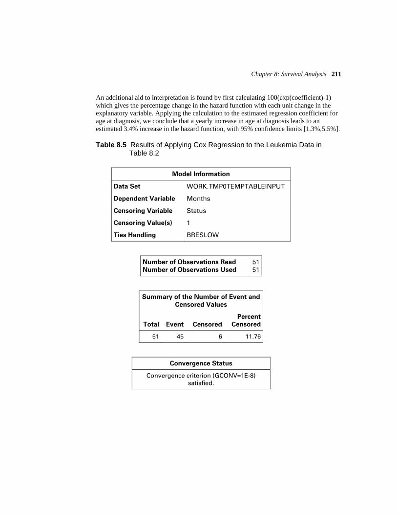
Chapter 8: Survival Analysis 211
An additional aid to interpretation is found by first calculating 100(exp(coefficient)-1) which gives the percentage change in the hazard function with each unit change in the explanatory variable. Applying the calculation to the estimated regression coefficient for age at diagnosis, we conclude that a yearly increase in age at diagnosis leads to an estimated 3.4% increase in the hazard function, with 95% confidence limits [1.3%,5.5%].
Table 8.5 Results of Applying Cox Regression to the Leukemia Data in Table 8.2
Model Information
Data Set WORK.TMP0TEMPTABLEINPUT
Dependent Variable Months
Censoring Variable Status
Censoring Value(s) 1
Ties Handling BRESLOW
Number of Observations Read
Number of Observations Used
5151
Summary of the Number of Event and
Censored Values
Total Event Censored
Percent
Censored
51 45 6 11.76
Convergence Status
Convergence criterion (GCONV=1E-8) satisfied.

212 Basic Statistics Using SAS Enterprise Guide: A Primer
Model Fit Statistics
Criterion
Without
Covariates
With
Covariates
-2 LOG L 291.106 276.086
AIC 291.106 286.086
SBC 291.106 295.120
Testing Global Null Hypothesis: BETA=0
Test Chi-Square DF Pr > ChiSq
Likelihood Ratio 15.0194 5 0.0103
Score 14.8274 5 0.0111
Wald 14.0130 5 0.0155
Analysis of Maximum Likelihood Estimates
Variable DF
Parameter
Estimate
Standard
Error Chi-Square Pr > ChiSq
Hazard
Ratio
95% Hazard
Ratio
Confidence
Limits
age 1 0.03359 0.01036 10.5140 0.0012 1.034 1.013 1.055
p_blasts 1 0.00928 0.01473 0.3968 0.5287 1.009 0.981 1.039
p_inf 1 -0.01613 0.01267 1.6195 0.2032 0.984 0.960 1.009
p_lab 1 -0.05386 0.03899 1.9086 0.1671 0.948 0.878 1.023
maxtemp 1 -0.0003663 0.00128 0.0820 0.7746 1.000 0.997 1.002

Chapter 8: Survival Analysis 213
8.4 Exercises
Exercise 8.1 The breast data set gives the survival times after mastectomy of women with breast cancer. Based on a histochemical marker, the cancers were classified as having metastasized or not. Censoring is indicated by an asterisk. Plot the product-limit estimates of the two survival functions on the same diagram, find the median survival times, and test for any difference in the survival experience of the two groups of women.
Not metastasized
23 47 69 70* 71* 100* 101* 148 181 198* 208* 212* 224*
Metastasized
5 8 10 13 18 24 26 26 31 35 40 41 48 50 59 61 68 71 76* 105* 107* 109* 113 116* 118 143 154* 162* 188* 212* 217* 225*
Exercise 8.2 The data in prostate arise from a randomized controlled trial to compare two treatments for prostrate cancer. Patients were randomized to receive either 1mg of diethylstilbestrol (DES) or 1mg of placebo daily by mouth, and their survival was recorded in months. The variables in the table below are as follows:
Treatment 0 = placebo, 1 = 1mg of diethylstillbeterol daily
Status 1 = dead, 0 = censored
Time Survival time in months
Age Age at trial entry in years
Haem Serum haemoglobin level in gm/100ml
Size Size of primary tumor in centimeters squared
Gleason the value of a combined index of tumor stage and grade (the larger the index, the more advanced the tumor)
Fit a Cox regression to the data and identify the most important prognostic variables for survival.

214 Basic Statistics Using SAS Enterprise Guide: A Primer
Prostate Cancer Trial Data
Treatment Time Status Age Haem Size Gleason
0 65 0 67 13.4 34 8 1 61 0 60 14.4 4 10 1 60 0 77 15.6 3 8
0 58 0 64 16.21 6 9 1 51 0 65 14.1 21 9
0 14 1 73 12.4 18 11 0 43 0 60 13.6 7 9
1 16 0 73 13.8 8 9 0 52 0 73 11.7 5 9
. . . . 1 67 0 73 13.8 7 8
0 23 0 68 12.5 2 8 0 62 0 63 13.2 3 8
Exercise 8.3 The data set Heroin gives the times that heroin addicts remained in a clinic for methadone treatment. If they were still in treatment at the end of the study, the status variable has a value 0. Potential explanatory variables for time to complete treatment are maximum methadone dose, clinic where treatment took place, and whether or not the addict had a criminal record; yes is coded one and no coded zero.
ID Clinic Status Time Prison Dose ID Clinic Status Time Prison Dose
1 1 1 428 0 50 132 2 0 633 0 70
2 1 1 275 1 55 133 2 1 661 0 40
3 1 1 262 0 55 134 2 1 232 1 70
4 1 1 183 0 30 135 2 1 13 1 60
5 1 1 259 1 65 137 2 0 563 0 70
6 1 1 714 0 55 138 2 0 969 0 80
. . . .
127 2 1 26 0 40 262 2 1 540 0 80
128 2 0 72 1 40 263 2 0 551 0 65
129 2 0 641 0 70 264 1 1 90 0 40 131 2 0 367 0 70 266 1 1 47 0 45

References
Agresti, A. 1996. Introduction to Categorical Data Analysis. New York: Wiley.
Aitkin, M. 1978. “The analysis of unbalanced cross classifications.” Journal of the Royal Statistical Society Series, Series A, Vol. 141, No. 2: 195–223.
Altman, D. G. 1991. Practical Statistics for Medical Research. 2d ed. London: CRC/Chapman and Hall.
Cleveland, W. S. 1994. The Elements of Graphing Data. Murray Hill, NJ: Hobart Press.
Collett, D. 2002. Modelling Binary Data. 2d ed. London: Chapman and Hall/CRC.
Collett, D. 2003. Modelling Survival Data in Medical Research. 2d ed. London: Chapman and Hall/CRC.
Cook, R. D. and Weisberg, S. 1982. Residuals and Influence in Regression. London: CRC/Chapman and Hall.
Cox, D. R. 1972. “Regression models and life tables.” Journal of the Royal Statistical Society, Series B, Vol. 34, No. 2: 187–200.
Der, G. and Everitt, B. S. 2005. Statistical Analysis of Medical Data Using SAS. London: Chapman and Hall/CRC.
Everitt, B. S. 1992. The Analysis of Contingency Tables. 2d ed. London: CRC/Chapman and Hall.
Everitt, B. S. 1994. Statistical Methods for Medical Investigations. 2d ed. London: Arnold.
Everitt, B. S. 1996. Making Sense of Statistics in Psychology: A Second-Level Course. Oxford: Oxford University Press.
Everitt, B. S. and Palmer, C. R. 2006. Encyclopaedic Companion to Medical Statistics. Arnold, London.
Everitt, B. S. and Rabe-Hesketh, S. 2001. Analyzing Medical Data Using S-PLUS. New York: Springer-Verlag.
Fisher, R. 1925. Statistical Methods for Research Workers. Edinburgh: Oliver and Boyd.
Hand, D. J., Daly, F., Lunn, D., McConway, K., and Ostrowski, E. 1993. A Handbook of Small Datasets. London: Chapman and Hall/CRC.
Howell, D. C. (1992). Statistical Methods for Psychologists. 3d ed. Belmont, CA: Duxbury Press.
Kaplan, E. L. and Meier, P. 1958. “Nonparametric estimation from incomplete observations.” Journal of the American Statistical Association, 53, No. 282: 457–481.

216 Basic Statistics Using SAS Enterprise Guide: A Primer
Kapor, M. 1981. “Efficiency on ergocycle in relation to knee-joint angle and drag.” Unpublished master’s dissertation, University of Delhi.
Kasser, I. and Bruce, R. A. 1969. “Comparative Effects of Aging and Coronary Heart Disease on Submaximal and Maximal Exercise.” Circulation, 39, 759–774.
Mallows, C. L. 1973. “Some comments on Cp.” Technometrics 15, No. 4: 661–675.
Mann, L. 1981. “The baiting crowds in episodes of threatened suicide.” Journal of Personality and Social Psychology, 41, 703–709.
Maxwell, S. E. and Delaney, H. D. 1990. Designing Experiments and Analyzing Data. Belmont, CA: Wadsworth.
Mehta, C. R. and Patel, N. R. 1986. “A hybrid algorithm for Fisher's exact test on unordered r × c contingency tables.” Communications in Statistics 15(2): 387–403.
Nelder, J. A. 1977. “A reformulation of linear models.” Journal of the Royal Statistical Society Series A, Vol. 140, No. 1: 48–77.
Rawlings, J. O., Sastry G. P. and Dickey, D. A. 2001. Applied Regression Analysis: A Research Tool. New York: Springer-Verlag. Rickman, R., Mitchell, N., Dingman, J., and Dalen, J. E. 1974. “Changes in serum cholesterol
during the Stillman diet.” Journal of the American Medical Association, 228, Issue 1: 54–58.
Scheffe, H. 1953. “A method for judging all contrasts in the analysis of variance.” Biometrika 40 (1-2): 87–110.
Tufte, E. R. 1983. The Visual Display of Quantitative Information. Cheshire, CT: Graphics Press.
Venables, W. N. and Ripley, B. D. 1994. Modern Applied Statistics with S-Plus. New York: Springer-Verlag.
Wetherill, G. B. 1982. Elementary Statistical Methods. 3d ed. London: Chapman and Hall/CRC.
Woodley, W. L., Simpson, J., Biondini, R., and Berkeley, J. 1977. “Rainfall results 1970–1975: Florida area cumulus experiment.” Science, 195, No. 4280: 735–742.

Index
A
active data set 8 ActiveX format 65 Advanced Expression Editor
access via New Advanced Filter button 20–21
creating variables 51 Data tab 17 depicted 17 Functions tab 17, 34–35 queries with conditional functions 20
age-specific failure rate 207 aliases, and folders 27 analysis of variance (ANOVA)
defined 112 F-test and 121, 123 heights and resting pulse rates 88 post-natal depression and child's IQ
124–133 simple linear regression and 88 sums of squares and 123 teaching arithmetic example 108–115 weight gain in rats 116–123
analysis tasks See statistical analysis
analysis variables 51, 109 Analyze menu
analysis tasks and 28 depicted 5 Linear Regression task 86–90 Logistic task 176, 180 One-Way ANOVA task 49, 113 statistical inference 43–46 Wilcoxon-Mann-Whitney test 49
ANOVA See analysis of variance
appending tables 21–26 ASCII files 8, 10
aspect ratio (scatterplots) 95–102 Assign Library wizard 27
B
balanced designs 130–131 bar charts 63–66 between groups variance 112 binary variables 158, 174 birthrates example 95–102 bivariate data
birthdates example 95–102 defined 81 heights and resting pulse rates 80–90 kinesiology experiment 90–94
box plots cloud seeding example 154–157 defined 37 room width estimates 36–38 teaching arithmetic example 109–111 wave power and mooring methods
50–54 weight gain in rats 116–119
brain tumors example chi-square test 70–71 example overview 68 null hypothesis 70 tabulating data into contingency table
69–71
C
categorical data brain tumors example 68–71 horse race winners 62–67 juvenile felons 75–77 Linear Models task 158 suicides and baiting behavior 71–75
categorical variables 62 censored observations 193, 201 censored survival times 192

218 Index
character values for variables 29 chi-square test for independence
brain tumors example 70–71 Fisher's exact test and 72 horse race winners example 66–67 suicide and baiting behavior 71–75
classification variables 29, 109 cloud seeding example
box plots 154–157 example overview 152–153 initial data examination 154–157 multiple regression with interaction
158–164 null hypothesis 153 residuals and 164–166 scatterplots 154–157, 163
comma-separated values 10, 141–142 Computed Columns icon (Query Builder
window) 16 Computed Columns window 17–18 concatenating data sets 21–26 conditional functions
building in Advanced Expression Editor 34–35
queries with 20 confidence intervals 42 contingency tables
chi-square test for independence 72 defined 69 Fisher's exact test and 72 tabulating data into 69–71
continuous variables 18–20 correlation coefficient
defined 82–85 heights and resting pulse rates 82–85 ice cream consumption 145 kinesiology example 92–93 linear relationships and 83 multiple linear regression and 145 nonlinear relationship and 83–84 Pearson's 82 product-moment 82
Cox regression 208–212 .csv file extension 10, 141–142
D
data description room width estimates 32–49 wave power and mooring methods
49–57 Data menu
analysis tasks 28 appending tables 21 creating variables 51 depicted 5 Filter and Query task 16, 22 sorting data 24
data sets active 8 concatenating 21–26 depicted in process flows 7–8 five-number summary 37 generating 8 icons for 8 importing 10–15 joining 21–26 listing for projects 22 manipulating in process flows 8 merging 21–26 modifying variables using queries 15–18 naming rules 22, 26–27 opening 9–10 recoding variables 18–20 renaming in process flows 25–26 sorting 24 splitting via filters 20–21 storing in libraries 27
database programs importing data from 14–15 raw data files and 10
death, hazard function for 207–208 degrees of freedom 66 delimited data 10–12 dependent variables 29

Index 219
Describe menu analysis tasks and 28 depicted 5 Distribution Analysis task 36, 149–150 One-Way Frequencies task 63–67 Summary Statistics task 35 Summary Tables task 109–110, 118,
126–127 Table Analysis task 69–71, 73, 76
discrete variables 29 Distribution Analysis task
accessing 36 box plots and 37, 51 probability plots 47 residual plots 149–150 summary statistics 35–36 Task Roles 36 Wilcoxon signed rank test 56–57
dummy variables 158, 185
E
end-of-line characters 10 equality of variance 48 explanatory variables
classification variables 29 Cox regression 208 logistic regression 175–179 multiple linear regression and 140, 146,
158 normal distribution and 144 residuals and 146
F
F-test analysis of variance and 121, 123 defined 88, 113 multiple linear regression and 144 one-way designs and 114
factor variables 112, 119 factorial designs 119–123 File menu
Import Data task 10, 14–15
opening data sets 3, 9, 15 opening process flows 51
Filter and Query task See also Query Builder window concatenating data sets 21–26 creating variables 51 merging data sets 21–26 modifying variables using queries 15–18 recoding variables 18–20 splitting data sets via filters 20–21
filters 20–21 Fisher, Ronald Aylmer 41, 112 Fisher's exact test 72–75 five-number summary (data sets) 37 fixed-width data 10–15 folders 27 frequency count variables 29
G
gastric cancer example overview 192–193 log-rank test 202–204 null hypothesis 202–203 survival function 193–204
gender as categorical variable 62 Graph menu
depicted 5 overview 30 selecting bar charts 63–64 selecting box plots 111, 117 selecting line plots 101 selecting pie charts 64 selecting scatterplots 81, 90, 97, 142
graphs See also box plots See also scatterplots bar charts 62–66 Distribution Analysis task 35–36 format dependencies 30 histograms 38–40, 146, 152 interaction plots 122–123 line plots 101 pie charts 62–66

220 Index
graphs (continued) stem-and-leaf plots 38–40, 146 summary statistics and 33–40
group analysis by variables 29
H
hazard function 193, 207–208 heights and resting pulse rates
correlation coefficient 82–85 example overview 80 null hypothesis 88 quantifying relationships between 82–85 scatterplots 81–82, 90 simple linear regression 85–90
histograms of residuals 146, 152 room width estimates 38–40
homogeneity assumption of F-test 114, 123 of one-way design 123 of t-test 48
horse race winners bar charts 62–66 chi-square test statistic 66–67 null hypothesis 66 pie charts 62–66
HTML output 30 hypothesis testing
See null hypothesis
I
ice cream consumption example overview 140–141 initial analysis 141–143 linear regression and 144–145, 158 multiple linear regression 143–146 null hypothesis 145 residuals 146–152 scatterplots 141–143
icons in process flow 7–8 Import Data task
alias support 27 Column Options pane 11, 13, 34
delimited data options 11 example 7 for fixed-width data 10–15 opening screen 11 Region to import pane 11 Results pane 11, 13–14 summary statistics 33–40 Text Format pane 11–12
independent samples t-test 45–47 inference
See statistical inference inputs to process flow 7–8 instantaneous death rate 207 instantaneous failure rate 207 interaction plots 122–123 interaction terms, multiple regression with
158–164 interquartile range 37
J
Join icon (Query Builder window) 23 joining data sets 21–26 juvenile felons example 75–77
K
Kaplan-Meier estimator 194 kinesiology example
example overview 90–91 scatterplots 91–93 simple linear regression 93–94
L
labels, naming rules 26–27 least squares estimation 86, 143 Lewis, T. 32 libraries 27 Life Tables task 194–202 likelihood ratio test 203 Line Plot task 101, 162 Linear Models task
Advanced Options 28–29 applying analysis of variance 120–121,
131–132

Index 221
diagnosing using residuals 164 example 7 finding analysis of variance table 128 interaction plots 122–123 Model Options pane 28–29 Model pane 28–29 multiple regression support 158 opening window depicted 28 Plots pane 28–29 Post Hoc Tests pane 28 Predictions pane 28 Task Roles pane 28–29 Titles pane 28
linear regression See multiple linear regression See simple linear regression
Linear Regression task heights and resting pulse rates 86–90 ice cream consumption 144–145, 158 plotting residuals 148
linear relationships 83 Local Computer 2, 9 log functions 17 log odds value 179–180, 185–186 log-rank test 202–204 logistic regression
defined 174 myocardial infarctions 172–186 regression coefficient 179–180, 185 single explanatory variable 175–179
Logistic task 176, 180 lower quartile 37
M
marital status as categorical variable 62 maximum value in five-number summary 37 McNemar's test 75–77 means
equality of 112 sample 41 Student's t-test 41, 112 teaching arithmetic example 109
median in five-number summary 37
menu bar 5 merging data sets 21–26 Microsoft Access 14–15 Microsoft Excel 14–15 minimum value in five-number summary 37 multiple comparison tests 114–115 multiple linear regression
cloud seeding example 152–166 defined 143 ice cream consumption 140–152 with interaction terms 158–164
myeloblastic leukemia Cox regression 208–212 example overview 204–206 hazard function 207–208 null hypothesis 210
myocardial infarctions example overview 172–173 logistic regression 174–186 null hypothesis 185 regression coefficient 179–180
N
naming rules 22, 26–27 New Advanced Filter button (Query Builder
window) 20–21 nonlinear relationships
heights and resting pulse rates 83–84 kinesiology example 91–93
normal distribution 47, 144 normality assumption
of F-test 114, 123 of one-way design 123 of t-test 48 residuals and 146–152
null hypothesis defined 41 of equality of means 113 p-value and 41–42 regression coefficient and 180 specifying value of 44 statistical inference and 41–47
numeric values for variables 17, 29

222 Index
O
odds ratio 179, 186 One-Way ANOVA task 49, 113 one-way designs 112–115 One-Way Frequencies task 63–67 outliers 36–37 outputs in process flow 7–8
P
p-value defined 41 F-test and 88, 113 Fisher's exact test 74 hypothesis testing and 42 significance tests and 41–42 sums of squares and 159 test for equality of variance and 48 test statistic and 71 Wilcoxon-Mann-Whitney test 203
paired t-test 54–57 parsimony, principle of 131 Pearson's correlation coefficient 82 pie charts 63–66 population, statistical inference 40–47 population sample 40, 62 post-natal depression and child's IQ
analysis of variance 128–133 example overview 124–125 null hypothesis 124 summary statistics 125–127
probability plots cloud seeding example 164–166 defined 47 room width estimates example 47–49
process flows activating 7 defined 6 examples 7–8 generating data sets 8 icons in 7–8 inputs to 7–8 opening 51 opening icons in 8
outputs to 7–8 renaming data sets in 25–26 renaming tasks in 25–26 running branches 30 running entire 30
product-limit estimator defined 194 of survival functions 195, 197–201
product-moment correlation coefficient 82 prognostic variables
See explanatory variables Project Designer window 5–7 Project Explorer window 5–6 projects
creating 9–15 defined 5 listing data sets 22 modifying data sets 15–27 opening data sets 9–10 statistical analysis tasks 28–29
proportional hazards model 209
Q
quantitative variables 29 queries
modifying variables via 15–18 with conditional functions 20
Query Builder window Computed Columns icon 16 creating variables 51 Filter Data tab 20–21, 42 filtering example 20–21 Join icon 23 joining data sets 23–26 New Advanced Filter button 20–21 room width estimates 34
R
R-square 89 raw data files 8, 10 regression coefficients
defined 159 in logistical regression 179–180, 185

Index 223
null hypothesis and 180 regression variance 144 relative weight variables 29 renaming
data sets in process flows 25–26 tasks in process flows 25–26
residuals cloud seeding example 164–166 ice cream consumption 146–152
response variables defined 112 factor variables and 112 logistic regression and 174 multiple linear regression and 140, 146 normal distribution and 144 residuals and 146
resting pulse rates See heights and resting pulse rates
right-censored survival times 192 right-click action (mouse)
modify joins 24 opening icons in process flow 8 opening tasks 18 renaming data sets in process flow 25 renaming tasks in process flow 25 running process flow 30
room width estimates checking assumptions 47–49 constructing box plots 37–38 constructing histograms 38–40 constructing stem-and-leaf plots 38–40 deriving summary statistics 35–36 example overview 32 initial analysis 33–40 null hypothesis 41 statistical inference 40–47
RTF output 30
S
sample, population 62 SAS data sets
See data sets SAS Enterprise Guide
applying Cox regression 209–212 applying logistical regression model
180–186 overview 2–3 plotting survival functions 194–202 starting connection 4 user interface 5–6
SAS Servers 2, 9 .sas7bdat file extension 9 SASUSER library 27 Satterthwaite test 46, 48 scatterplots
aspect ratio of 95–102 birthrates example 95–102 bivariate data and 81–82 cloud seeding example 154–157, 163 heights and resting pulse rates 81–82, 90 ice cream consumption 141–143, 145 kinesiology example 91–93
Scheffe's method 114–115 .sd2 file extension 9 settings, manipulating 3–4 significance tests 40–42 simple linear regression
defined 85–90 heights and resting pulse rates 85–90 kinesiology example 93–94
skewed guesses 37, 192 social class as categorical variable 62 sorting data sets 24 spaces
in delimited data 10 in labels 27 in raw data files 10
special characters in delimited data 10 spreadsheets
importing data from 14–15 raw data files and 10
standard deviations in logistical regression 186 teaching arithmetic example 109 test statistic from 41 weight gain in rats 119

224 Index
statistical analysis birthdates example 95–102 brain tumors example 68–71 cloud seeding example 152–166 gastric cancer 192–204 heights and resting pulse rates 80–90 horse race winners 62–67 ice cream consumption 140–152 juvenile felons 75–77 kinesiology experiment 90–94 myeloblastic leukemia 204–212 myocardial infarctions 172–186 overview 28–29 post-natal depression and child's IQ
124–133 room width estimates 32–49 suicides and baiting behavior 71–75 teaching arithmetic example 108–115 wave power and mooring methods 49–57 weight gain in rats 116–123
statistical inference defined 40 room width estimates 32–49 wave power and mooring methods 49–57
Statistical Methods for Research Workers (Fisher) 41
statistical tests chi-square test 66–67, 70–75 F-test 88, 113–114, 121, 123, 144 Fisher's exact test 72–75 hypothesis testing 41–47 independent samples t-test 45–47 likelihood ratio test 203 log-rank test 202–204 McNemar's test 75–77 multiple comparison tests 114–115 paired t-test 54–57 Satterthwaite test 46, 48 Scheffe's method 114–115 significance tests 40–42 Student's t-test 41–47, 85, 112 test for equality of variance 48 Wilcoxon-Mann-Whitney test 49, 203
Wilcoxon signed rank test 56–57 stem-and-leaf plots
of residuals 146 room width estimates 38–40
stored data in libraries 27 location of 9
Student's t-test heights and resting pulse rates 85 population means and 41, 112 purpose 41 room width estimates 41–47
suicides and baiting behavior example overview 71 Fisher's exact test 72–75 null hypothesis 72
summary statistics deriving 33, 35–36 Distribution Analysis task 35–36 graphics and 33–40 numerical data 116–119 post-natal depression and child's IQ
125–127 teaching arithmetic example 109–111
Summary Statistics task 35 Summary Tables task
example 7 post-natal depression and child's IQ
126–127 teaching arithmetic example 109–110 weight gain in rats 118
sums of squares analysis of variance and 123 post-natal depression and child's IQ 130 Type I 123, 130–131, 159 Type III 123, 130–131, 159 Type IV 130
survival analysis gastric cancer 192–204 myeloblastic leukemia 204–212
survival functions defined 193–194 plotting 194–202

Index 225
survival times censored 192 defined 193 likelihood ratio test 203 mean 199 median 195
T
t-test independent samples 45–47 paired 54–57 regression coefficient and 159 Student's 41–47
Table Analysis task brain tumors example 68–71 juvenile felons example 75 suicides and baiting behavior 73
Tables and Join window 24 tabs
in delimited data 10 in raw data files 10
Task List window 5–6 Task Status window 5–6 tasks
defined 6 in process flow example 7 manipulating in process flows 8 naming rules 26–27 performing 3 renaming in process flows 25–26 running from process flows 30
teaching arithmetic example box plots 109–111 example overview 108 initial data examination 109–111 null hypothesis 112 one-way design 112–115 summary statistics 109–111
temporary library 27 test statistic 41, 72 text files 8, 10 toolbar 5–6 Tools menu
assigning libraries 27 manipulating graph format 30, 65 manipulating results format 30 manipulating settings 3–4, 16
Type I sums of squares cloud seeding example 159 defined 123 post-natal depression and child's IQ
130–131 Type III sums of squares
cloud seeding example 159 defined 123 post-natal depression and child's IQ
130–131 Type IV sums of squares 130
U
unbalanced design 127 upper quartile
in five-number summary 37 interquartile range and 37
user interface 5–6
V
variable selection methods 158 variables
See also explanatory variables See also response variables analysis 51, 109 binary 158, 174 categorical 62 character values 29 classification 29, 109 continuous 18–20 correlation coefficient and 83 creating 17, 51 delimited files and 10 dependent 29 discrete 29 dummy 158, 185 factor 112, 119 frequency count 29 group analysis by 29

226 Index
variables (continued) modifying via queries 15–18 naming rules 26–27 numeric values 17, 29 quantitative 29 recoding 18–20 relative weight 29 selecting for analysis 29
variance between groups 112 equality of 48 factor variables and 112 R-square and 89 regression 144 residuals and 146–152 t-test assumptions 47–48 within groups 112
Venn diagrams 24
W
wave power and mooring methods checking assumptions 56–57 example overview 49–50 initial analysis 50–54 null hypothesis 55 testing differences 54–56
weight gain in rats box plots 116–119 example overview 116 factorial designs 119–123 interaction plots 122–123 numerical summaries 116–119
Welcome Screen 4 Wilcoxon-Mann-Whitney test 49, 203 Wilcoxon signed rank test 56–57 within groups variance 112 WORK library 27

Books Available from SAS Press
Advanced Log-Linear Models Using SAS®
by Daniel Zelterman
Analysis of Clinical Trials Using SAS®: A Practical Guideby Alex Dmitrienko, Geert Molenberghs, Walter Offen, and Christy Chuang-Stein
Analyzing Receiver Operating Characteristic Curves with SAS®
by Mithat Gönen
Annotate: Simply the Basicsby Art Carpenter
Applied Multivariate Statistics with SAS® Software,Second Editionby Ravindra Khattreeand Dayanand N. Naik
Applied Statistics and the SAS® Programming Language, Fifth Editionby Ronald P. Cody and Jeffrey K. Smith
An Array of Challenges — Test Your SAS® Skillsby Robert Virgile
Basic Statistics Using SAS® Enterprise Guide®: A Primerby Geoff Derand Brian S. Everitt
Building Web Applications with SAS/IntrNet®: A Guide to the Application Dispatcherby Don Henderson
Carpenter’s Complete Guide to the SAS® Macro Language, Second Edition by Art Carpenter
Carpenter’s Complete Guide to the SAS® REPORT Procedure by Art Carpenter
The Cartoon Guide to Statistics by Larry Gonick and Woollcott Smith
Categorical Data Analysis Using the SAS® System, Second Editionby Maura E. Stokes, Charles S. Davis, and Gary G. Koch
Cody’s Data Cleaning Techniques Using SAS® Software by Ron Cody
Common Statistical Methods for Clinical Research with SAS® Examples, Second Editionby Glenn A. Walker
The Complete Guide to SAS® Indexesby Michael A. Raithel
CRM Segmemtation and Clustering Using SAS® Enterprise MinerTM
by Randall S. Collica
Data Management and Reporting Made Easy with SAS® Learning Edition 2.0by Sunil K. Gupta
Data Preparation for Analytics Using SAS®
by Gerhard Svolba
Debugging SAS® Programs: A Handbook of Tools and Techniquesby Michele M. Burlew
support.sas.com/publishing

Decision Trees for Business Intelligence and Data Mining: Using SAS® Enterprise MinerTM
by Barry de Ville
Efficiency: Improving the Performance of Your SAS® Applicationsby Robert Virgile
The Essential Guide to SAS® Dates and Timesby Derek P. Morgan
Fixed Effects Regression Methods for Longitudinal Data Using SAS®
by Paul D. Allison
Genetic Analysis of Complex Traits Using SAS®
by Arnold M. Saxton
A Handbook of Statistical Analyses Using SAS®, Second Editionby B.S. Everittand G. Der
Health Care Data and SAS® by Marge Scerbo, Craig Dickstein, and Alan Wilson
The How-To Book for SAS/GRAPH® Softwareby Thomas Miron
In the Know... SAS® Tips and Techniques From Around the Globe, Second Editionby Phil Mason
Instant ODS: Style Templates for the Output Delivery Systemby Bernadette Johnson
Integrating Results through Meta-Analytic Review UsingSAS® Softwareby Morgan C. Wangand Brad J. Bushman
Introduction to Data Mining Using SAS® Enterprise MinerTM
by Patricia B. Cerrito
Introduction to Design of Experiments with JMP® Examples, Third Editionby Jacques Goupyand Lee Creighton
Learning SAS® by Example: A Programmer’s Guideby Ron Cody
The Little SAS® Book: A Primerby Lora D. Delwiche and Susan J. Slaughter
The Little SAS® Book: A Primer, Second Editionby Lora D. Delwiche and Susan J. Slaughter (updated to include SAS 7 features)
The Little SAS® Book: A Primer, Third Editionby Lora D. Delwiche and Susan J. Slaughter(updated to include SAS 9.1 features)
The Little SAS® Book for Enterprise Guide® 3.0by Susan J. Slaughterand Lora D. Delwiche
The Little SAS® Book for Enterprise Guide® 4.1by Susan J. Slaughterand Lora D. Delwiche
Logistic Regression Using the SAS® System:Theory and Applicationby Paul D. Allison
Longitudinal Data and SAS®: A Programmer’s Guideby Ron Cody
Maps Made Easy Using SAS®
by Mike Zdeb
Measurement, Analysis, and Control Using JMP®: Quality Techniques for Manufacturingby Jack E. Reece
Multiple Comparisons and Multiple Tests Using SAS® Text and Workbook Set(books in this set also sold separately)by Peter H. Westfall, Randall D. Tobias,Dror Rom, Russell D. Wolfinger,and Yosef Hochberg
support.sas.com/publishing

Multiple-Plot Displays: Simplified with Macrosby Perry Watts
Multivariate Data Reduction and Discrimination with SAS® Softwareby Ravindra Khattreeand Dayanand N. Naik
Output Delivery System: The Basicsby Lauren E. Haworth
Painless Windows: A Handbook for SAS® Users,Third Editionby Jodie Gilmore(updated to include SAS 8 and SAS 9.1 features)
Pharmaceutical Statistics Using SAS®: A Practical GuideEdited by Alex Dmitrienko, Christy Chuang-Stein, and Ralph D’Agostino
The Power of PROC FORMATby Jonas V. Bilenas
Predictive Modeling with SAS® Enterprise MinerTM: Practical Solutions for Business Applicationsby Kattamuri S. Sarma
PROC SQL: Beyond the Basics Using SAS® by Kirk Paul Lafler
PROC TABULATE by Exampleby Lauren E. Haworth
Professional SAS® Programmer’s Pocket Reference, Fifth Editionby Rick Aster
Professional SAS® Programming Shortcuts, Second Editionby Rick Aster
Quick Results with SAS/GRAPH® Softwareby Arthur L. Carpenter and Charles E. Shipp
Quick Results with the Output Delivery System by Sunil Gupta
Reading External Data Files Using SAS®: Examples Handbookby Michele M. Burlew
Regression and ANOVA: An Integrated Approach Using SAS® Softwareby Keith E. Muller and Bethel A. Fetterman
SAS® For Dummies®
by Stephen McDanieland Chris Hemedinger
SAS® for Forecasting Time Series, Second Editionby John C. Brocklebankand David A. Dickey
SAS® for Linear Models, Fourth Editionby Ramon C. Littell, Walter W. Stroup,and Rudolf Freund
SAS® for Mixed Models, Second Editionby Ramon C. Littell, George A. Milliken, Walter W. Stroup, Russell D. Wolfinger, and Oliver Schabenberger
SAS® for Monte Carlo Studies: A Guide for Quantitative Researchersby Xitao Fan, Ákos Felsovályi, Stephen A. Sivo,and Sean C. Keenan
SAS® Functions by Exampleby Ron Cody
SAS® Graphics for Java: Examples Using SAS® AppDev StudioTM and the Output Delivery Systemby Wendy Bohnenkampand Jackie Iverson
SAS® Guide to Report Writing, Second Editionby Michele M. Burlew
SAS® Macro Programming Made Easy, Second Editionby Michele M. Burlew
SAS® Programming by Exampleby Ron Codyand Ray Pass
support.sas.com/publishing
˝

SAS® Programming for Enterprise Guide® Usersby Neil Constable
SAS® Programming in the Pharmaceutical Industryby Jack Shostak
SAS® Survival Analysis Techniques for Medical Research, Second Editionby Alan B. Cantor
SAS® System for Elementary Statistical Analysis,Second Editionby Sandra D. Schlotzhauerand Ramon C. Littell
SAS® System for Regression, Third Editionby Rudolf J. Freund and Ramon C. Littell
SAS® System for Statistical Graphics, First Editionby Michael Friendly
The SAS® Workbook and Solutions Set (books in this set also sold separately)by Ron Cody
Saving Time and Money Using SAS®
by Philip R. Holland
Selecting Statistical Techniques for Social Science Data: A Guide for SAS® Usersby Frank M. Andrews, Laura Klem, Patrick M. O’Malley, Willard L. Rodgers, Kathleen B. Welch,and Terrence N. Davidson
Statistics Using SAS® Enterprise Guide®
by James B. Davis
A Step-by-Step Approach to Using the SAS® Systemfor Factor Analysis and Structural Equation Modelingby Larry Hatcher
A Step-by-Step Approach to Using SAS® for Univariate and Multivariate Statistics, Second Editionby Norm O’Rourke, Larry Hatcher,and Edward J. Stepanski
support.sas.com/publishing
Step-by-Step Basic Statistics Using SAS®: StudentGuide and Exercises(books in this set also sold separately)by Larry Hatcher
Survival Analysis Using SAS®:A Practical Guideby Paul D. Allison
Tuning SAS® Applications in the OS/390 and z/OS Environments, Second Editionby Michael A. Raithel
Using SAS® in Financial Researchby Ekkehart Boehmer, John Paul Broussard,and Juha-Pekka Kallunki
Visualizing Categorical Databy Michael Friendly
Web Development with SAS® by Example, Second Editionby Frederick E. Pratter
JMP® Books
Elementary Statistics Using JMP®
by Sandra D. Schlotzhauer
JMP® for Basic Univariate and Multivariate Statistics: A Step-by-Step Guideby Ann Lehman, Norm O’Rourke, Larry Hatcher,and Edward J. Stepanski
JMP® Start Statistics: A Guide to Statistics and Data Analysis Using JMP®, Fourth Editionby John Sall, Lee Creighton,and Ann Lehman
Regression Using JMP®
by Rudolf J. Freund, Ramon C. Littell,and Lee Creighton


