download unit 30 student guide

Unit 30: Inference for Regression | Student Guide |

Summary of VideoIn Unit 11, Fitting Lines to Data, we examined the relationship between winter snowpack and spring runoff. Colorado resource managers made predictions about the seasonal water supply using a least-squares regression line that was fit to a scatterplot of their measurement data, which is shown in Figure 30.1.

Figure 30.1. Least-squares regression line used by Colorado resource managers.

But would we really see a linear relationship between snowpack and runoff if we had all the possible data? Or might the pattern we see in the sample data’s scatterplot occur just by chance? We would like to know whether the positive association we see between snowpack and runoff in the sample is strong enough that we can conclude that the same relationship holds for the whole population. Statisticians rely on inference to determine whether the relationship observed between two variables in a sample is valid for some larger population.

Inference is a powerful tool. Powerful enough, in fact, to help bring an entire bird species back from the brink of extinction. After World War II, the agrichemical industry began mass-producing chemicals to control pests. Cities like San Antonio, Texas, sprayed whole sections of the city with the insecticide DDT in their fight against the spread of poliomyelitis. Unfortunately,

Unit 30: Inference for Regression


there weren’t many safeguards in place, and the damaging environmental effects of these compounds were not taken into account. Eventually, changes in the natural environment due to chemical pesticides became apparent. One species that was severely affected was the peregrine falcon.

In Great Britain, Derek Ratcliffe noticed in the 1950s that peregrine falcons were declining at nesting sites and they were unable to hatch their eggs. This decline in falcons was eventually demonstrated to be a worldwide phenomenon. Researchers determined that the reason peregrine falcons were not successfully hatching their eggs was due to eggshell thinning, a very serious problem since the weaker shells were breaking before the baby birds were ready to hatch. After looking at some of the causes for this eggshell thinning, scientists began to zero in on a possible culprit: DDT and its breakdown product, DDE.

There were a couple of reasons why scientists believed that there was a relationship between DDT or DDE and eggshell thinning. In studying the broken eggshells and eggs collected in the field, scientists found very high residues of DDE that had not been seen in historic samples. The falcons were ingesting DDT through their prey – birds they ate had small concentrations of the chemical in their flesh. Over time the DDT built up in the peregrines’ own bodies and started to affect the females’ ability to lay healthy eggs.

Even though scientists had a pretty strong hunch that DDT was the cause of peregrine falcon eggshell thinning, they could not rely on their scientific instincts alone. So, researchers turned to statistics as a way to validate their analyses. We can follow in the researchers’ footsteps by taking a look at a data set comprised of 68 peregrine falcon eggs from Alaska and Northern Canada. A scatterplot of the two variables we will be studying, eggshell thickness (response variable) and the log-concentration of DDE (explanatory variable), appears in Figure 30.2. We have added the least-squares regression line fit to these data. Remember it is described by an equation of the form y a bx= + .


Figure 30.2. Scatterplot of eggshell thickness versus log-concentration of DDE.

The data in Figure 30.2 show a negative, linear relationship between the two variables. Using the equation, we can predict eggshell thickness for any measurement of DDE. The slope b and intercept a are statistics, meaning we calculated them from our sample data. But if we repeated the study with a different sample of eggs, the statistics a and b would take on somewhat different values. So, what we want to know now is whether there really is a negative linear relationship between these variables for the entire population of all peregrine eggs, beyond just the eggs that happen to be in our sample. Or might the pattern we see in the sample data be due simply to chance variation?

Data of the entire peregrine egg population might look like the scatterplot in Figure 30.3. Notice that for any given value of the explanatory variable, such as the value indicated by the vertical line, many different eggshell thicknesses may be observed.

Figure 30.3. Scatterplot representing population of peregrine eggs.


In the scatterplot in Figure 30.4, the mean eggshell thickness, y, does have a linear relationship with the log concentration of DDE, x. The line fit to the hypothetical population data is called the population regression line. Because we don’t have access to ALL the population data, we use our sample data to estimate the population regression line.

Figure 30.4. The population regression line fit to the population data.

Several conditions, which are discussed in the Content Overview, must be met in order to move forward with regression inference. You can check out whether these conditions are satisfied in Review Question 1. But for now, we assume that the conditions for inference are met. The population regression model is written as follows:

µy = α + βx

where y represents the true population mean of the response y for the given level of x, α is the population y-intercept, and β is the population slope. Now let’s look back at our least squares regression line, based on the sample of 68 bird eggs. The equation is

ˆ 2.146 0.3191y x= −

The sample intercept, a = 2.146, is an estimate for the population intercept α . And the sample slope, b = -0.3191, is an estimate for the population slope β.

Of course, we’ve learned by now that other samples from the same population will give us different data, resulting in different parameter estimates of α and β. In repeated sampling, the value of these statistics, a and b, form sampling distributions, which provide the basis for statistical inference. In particular, we want to infer from the sampling distribution for our statistic b, whether the sample data provide sufficiently strong evidence that higher levels of DDE are


related to eggshell thinning in the population. To answer this question, we set up our null and alternative hypotheses.

:oH Amount of DDE and eggshell thickness have no linear relationship.

or H0 :β = 0

:aH Amount of DDE and eggshell thickness have a negative linear relationship.

or Ha :β < 0

The t-test statistic for testing the null hypothesis is:

t =b − β0sb

where b is our sample estimate for the population slope, β0 is the null hypothesis value for the population slope, and bs is the standard error of the estimate b, which we can get from software. In this case, 0.0255bs = . Next, we calculate the value of our t-test statistic:

0.3191 0 12.50.0255

t − −= ≈ −

If the null hypothesis is true, then t has a t-distribution with n – 2, or 66, degrees of freedom. The value t = -12.5 is an extreme value and the corresponding p-value is essentially 0. Thus, we have strong evidence to reject the null hypothesis. By rejecting the null hypothesis, we can confirm what scientists already suspected – that there is a connection between peregrine falcon eggshell thickness and the presence of DDE. More precisely, there is a statistically significant, negative linear relationship between the log-concentration of DDE and the thickness of peregrine eggshells.

Before researchers could present this finding to the public, however, they had to quantify the relationship. That meant computing a confidence interval for the population slope. Here’s the formula:

* bb t s±

For a 95% confidence interval and df = 68 – 2 = 66, we find t* = 1.997. Now, we can compute the confidence interval:


0.3191 (1.997)(0.0255)− ±

3.191 0.0509− ±

0.3700 to 0.2681− −

Hence, based on our sample of 68 peregrine falcon eggs, we are 95% confident that a one-unit increase in the log-concentration of DDE is associated with a true average decrease of between 0.27 and 0.37 in Ratcliffe’s eggshell thickness index. Armed with this information, scientists were able to make a strong argument against the use of DDT because of its dangerous impact on peregrines and the environment as a whole. These results led to a prolonged legal battle with people on both sides presenting evidence. Due to scientific and statistical evidence, the United States and many Western European countries banned DDT use. Since then, the peregrine falcon population has rebounded significantly. So, this environmental detective story has a happy ending for the peregrine falcons.


Student Learning Objectives

A. Understand the linear regression model. Know how to find the least-squares regression line as an estimate (covered in Unit 11, Fitting Lines to Data.)

B. Know how to check whether the assumptions for the linear regression model are reasonably satisfied.

C. Recall how to find the least-squares regression equation (Unit 11, Fitting Lines to Data).

D. Be able to calculate, or obtain from software, the standard error of the estimate, es , and the standard error of the slope, bs .

E. Be able to conduct a significance test for the population slope β.

F. Be able to calculate a confidence interval for the population slope β.


Content Overview

While we often hear of the benefits of eating fish, we also hear warnings about limiting our consumption of certain fish whose flesh contains high levels of mercury. Much like the peregrine falcons and DDT, small levels of mercury in oceans, lakes, and streams build up in fish tissue over time. It becomes most concentrated in larger fish, which are higher up on the food chain.

To better understand the relationship between fish size and mercury concentration, the United State Geological Survey (USGS) collected data on total fish length and mercury concentration in fish tissue. (Total length is the length from the tip of the snout to the tip of the tail.) The data from a sample of largemouth bass (of legal size to catch) collected in Lake Natoma, California, appear in Table 30.1. (You may remember these data from Review Question 3 in Unit 11.)

Table 30.1. Fish total length and mercury concentration in fish tissue.

Since we believe that fish length explains mercury concentration, total length is the explanatory variable and mercury concentration is the response variable. A scatterplot of mercury concentration versus total length appears in Figure 30.5.

Total Length Mercury Concentration Total Length Mercury Concentration(mm) (µg/g wet wt.) (mm) (µg/g wet wt.)341 0.515 490 0.807353 0.268 315 0.320387 0.450 360 0.332375 0.516 385 0.584389 0.342 390 0.580395 0.495 410 0.722407 0.604 425 0.550415 0.695 480 0.923425 0.577 448 0.653446 0.692 460 0.755

Table 30.1


Figure 30.5. Scatterplot of mercury concentration versus total fish length.

Since the pattern of the dots in the scatterplot indicates a positive, linear relationship between the two variables, we fit a least-squares line to the data. However, these data are a sample of 20 largemouth bass from the population of all the largemouth bass that live in Lake Natoma. While we can use the least-squares equation to make predictions about mercury concentration for fish of a particular length, we need techniques from statistical inference to answer the following questions about the population:

• Is there really a positive linear relationship between the variables mercury concentration and total length, or might the pattern observed in the scatterplot be due simply to chance?

• Can we determine a confidence interval estimate for the population slope, the rate of change of mercury concentration per one millimeter increase in fish total length?

• If we use the least-squares line to predict the mercury concentration for a fish of a particular length, how reliable is our prediction?

Now, what if we could make a scatterplot of mercury concentration versus total length for all of the largemouth bass (at or close to the legal catch length) in Lake Natoma? Figure 30.6 shows how a scatterplot of the population might look and how a regression line fit to the population data might look.

500450400350300

1.0

0.9

0.8

0.7

0.6

0.5

0.4

0.3

0.2

Total Length (mm)

Mer

cury

Con

cent

ratio

n (µ

g/g)

y = - 0.7374 + 0.003227x


Figure 30.6. Population scatterplot of mercury concentration versus total length.

Notice, for each fish length, x, there are many different values of mercury concentration, y. For example, in Figure 30.6 a vertical line segment has been drawn at length 1x . That line segment intersects with a whole distribution of mercury concentration values, y-values, on the scatterplot. The mean of that distribution of y-values, µy , is at the intersection of the vertical line at 1x and the regression line. Now look at the vertical line at 2x . It too intersects with an entire distribution of y-values, with mean at the intersection of the vertical line at

2x and the regression line. So, the population regression line describes how the mean mercury concentration values, µy , are related to total length, x. In this case, the relationship looks linear and so we express it as: µy = α + βx . As mentioned earlier in this unit, several conditions must be met in order to move forward with regression inference. Those conditions, along with a description of the simple linear regression model, are presented below.

600500400300200

1.25

1.00

0.75

0.50

0.25

0.00

Total Length (mm)

Mer

cury

Con

cent

ratio

n µ

g/g

Population Scatterplot

x x1 2

y xµ α β= +


Simple Linear Regression Model and Conditions

We have n ordered pairs of observations (x, y) on an explanatory variable, x, and response variable, y.

The simple linear regression model assumes that for each value of x the observed values of the response variable, y, vary about a mean µy that has a linear relationship with x:

µy = α + βx

The line described by µy = α + βx is called the population regression line. In addition, the following conditions must be satisfied:

• For any fixed value of x, the response y varies according to a normal distribution. Repeated responses, y-values, are independent of each other.

• The standard deviation of y for any value of x, σ , is the same for all values of x.

Thus, the model has three unknown population parameters: α, β, and σ .

Figure 30.7 provides a graphic representation of the simple linear regression model and conditions.

x x x1 2 3

yµ = α + βx

x

y

α + βx

α + βx

α + βx1

2

3

Three different x-values

σ

σ

σ

Figure 30.7. Graphic representation of linear regression model.

A first step in inference is to estimate the unknown parameters. We begin with estimates for the slope and intercept of the population regression line. The estimated regression line for the linear regression model is the least-squares line, y a bx= + . From Figure 30.5, the estimated regression line is:


ˆ 0.7374 0.003227y x= − +

The y-intercept, a = -0.7374, is a point estimate for the population intercept, α , and the slope, b = 0.003227, is a point estimate of the population slope, β.

Next, we develop an estimate for σ , which measures the variability of the response y about the population regression line. Because the least-squares line estimates the population regression line, the residuals estimate how much y varies about the population regression line:

residual = observed y – predicted y

= ˆy y−

We estimate σ from the standard deviation of the residuals, es , as follows:

2ˆ( ) SSE2 2e

y ys

n n−

= =− −

∑

Our estimate for σ , es , is called the standard error of the estimate.

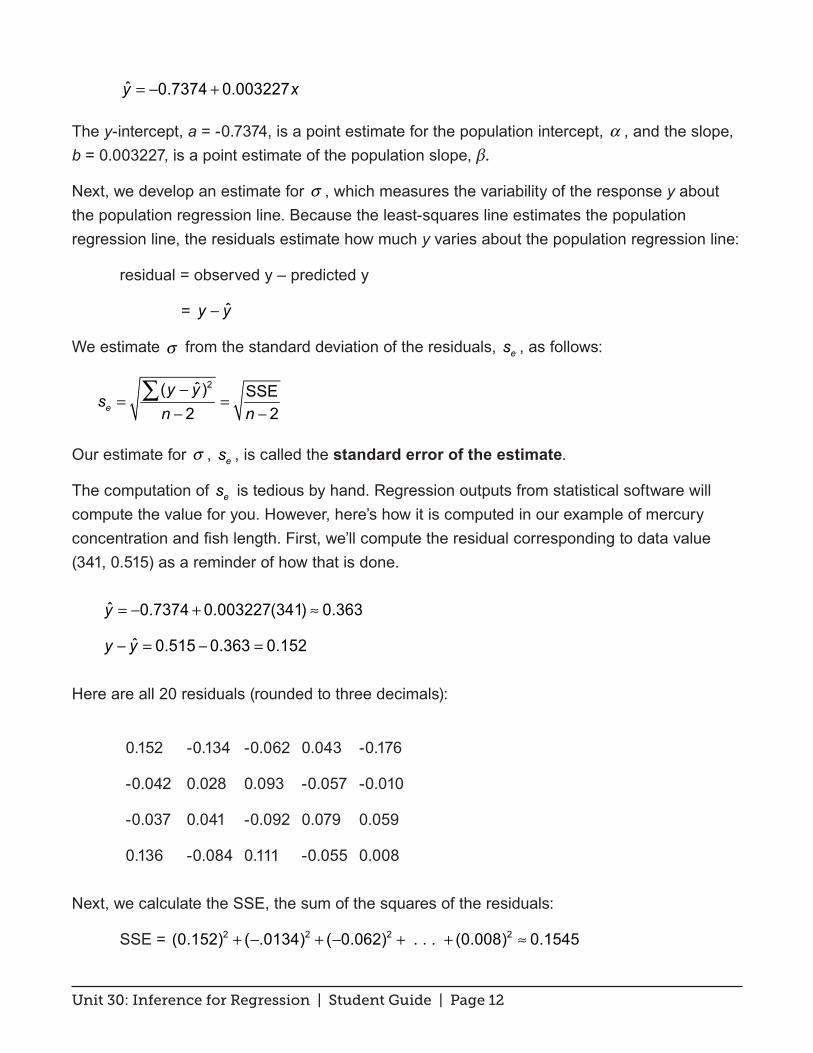
The computation of es is tedious by hand. Regression outputs from statistical software will compute the value for you. However, here’s how it is computed in our example of mercury concentration and fish length. First, we’ll compute the residual corresponding to data value (341, 0.515) as a reminder of how that is done.

ˆ 0.7374 0.003227(341) 0.363y = − + ≈

ˆ 0.515 0.363 0.152y y− = − =

Here are all 20 residuals (rounded to three decimals):

0.152 -0.134 -0.062 0.043 -0.176

-0.042 0.028 0.093 -0.057 -0.010

-0.037 0.041 -0.092 0.079 0.059

0.136 -0.084 0.111 -0.055 0.008

Next, we calculate the SSE, the sum of the squares of the residuals:

SSE = 2 2 2 2(0.152) ( .0134) ( 0.062) . . . (0.008) 0.1545+ − + − + + ≈


Now, we calculate es :

SSE 0.1545 0.092620 2 18es = ≈ ≈

− μg/g

We can use the equation of the least-squares line, ˆ 0.7374 0.003227y = − + , to make predictions. However, those predictions are more reliable when the data points lie “close” to the line. Keep in mind that es is one measure of the closeness of the data to the least-squares line. If 0es = , the data points fall exactly on the least-squares line. Moreover, when es is positive, we can use it to place error bounds above and below the least-squares line. These error bounds are lines parallel to the least-squares line that lie one or two es above and below the least-squares line. We apply this idea to our mercury concentration and fish length data.

ˆ 0.7374 0.003227 0.0926y x= − + ±

ˆ 0.7374 0.003227 2(0.0926)y x= − + ±

Figure 30.8. Adding lines ± es and ±2 es above and below the least-squares line.

Recall from Unit 8, Normal Calculations, that we expect roughly 68% of normal data to lie within one standard deviation of the mean and roughly 95% to lie within two standard deviations of the mean. Notice that all of our data fall within two es of the least-squares line. So, for a particular fish length, say with total length = 400 mm, we expect roughly 95% of the fish to have mercury concentrations between 0.3682 μg/g and 0.7386 μg/g.

The standard error of the estimate provides one way to select between competing models. For example, suppose we had a second model relating mercury concentration to the explanatory variable fish weight. Choose the model with the smaller value for es .

500450400350300

1.0

0.9

0.8

0.7

0.6

0.5

0.4

0.3

0.2

0.1

Total Length (mm)

Mer

cury

Con

cent

ratio

n (

µg/g

)


The scatterplot in Figure 30.5 appears to support the hypothesis that longer fish tend to have higher levels of mercury concentration. But is this positive association statistically significant? Or could it have occurred just by chance? To answer this question, we set up the following null and alternative hypotheses:

H0 : Total length and mercury concentration have no linear relationship. or H0 :β = 0

: Total length and mercury concentration have a positive linear relationship.aH

or Ha :β > 0

A regression line with slope 0 is horizontal. That indicates that the mean of the response y does not change as x changes – which, in turn, means that the linear regression equation is of no value in predicting y. In the case of mercury concentration and total length, the estimate of the population slope is very small, b = 0.003227. So, we might jump to the conclusion that total length is not useful in predicting mercury concentration. But we’d better work through the details of a significance test before jumping to such a conclusion.

Significance Test For Regression Slope, β

To test the hypothesis H0 :β = β0 , compute the t-test statistic:

t =b − β0s b

where 2( )

eb

ssx x

=−∑

and b is the least-squares estimate of the population slope, β, and β0 is the null hypothesis value for β .

If the null hypothesis is true and the linear regression conditions are satisfied, then t has a t-distribution with df = n – 2.

Back to the situation with mercury concentration and fish length. We use software to help us calculate bs :

0.093 0.00046839463.2bs = ≈


Now we are ready to calculate t:

0.003227 0 6.90.000468

t −= ≈

In this case, df = n – 2 = 20 – 2 = 18. Since this is a one-sided alternative, we find the probability of observing a value of t at least as large as the one we observed, 6.9. As shown in Figure 30.9, the area under the t-density curve to the right of 6.9 is so small that it isn’t really visible. The area is only 9.4127 × 10-7; so, p ≈ 0. We conclude that there is sufficient evidence to reject the null hypothesis and conclude β > 0. There is a positive linear relationship between total length and mercury concentration.

Figure 30.9. Calculating the p-value.

Next, we calculate a confidence interval estimate for the regression slope, β. Here are the details for constructing a confidence interval.

Confidence Interval For Regression Slope, β

A confidence interval for β is computed using the following formula:

* bb t s±

where t* is a t-critical value associated with the confidence level and determined from a t-distribution with df = n – 2; b is the least-squares estimate of the population slope, and bs is the standard error of b.

t

9.4127E-07

0 6.9

Density Curve for t-distribution, df = 18


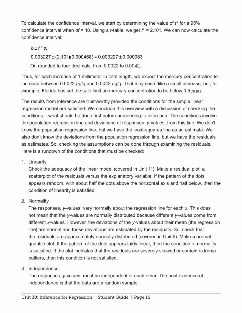
To calculate the confidence interval, we start by determining the value of t* for a 95% confidence interval when df = 18. Using a t-table, we get t* = 2.101. We can now calculate the confidence interval:

* bb t s±

0.003227 (2.101)(0.000468) 0.003227 0.000983± ≈ ± ,

Or, rounded to four decimals, from 0.0022 to 0.0042.

Thus, for each increase of 1 millimeter in total length, we expect the mercury concentration to increase between 0.0022 μg/g and 0.0042 μg/g. That may seem like a small increase, but, for example, Florida has set the safe limit on mercury concentration to be below 0.5 μg/g.

The results from inference are trustworthy provided the conditions for the simple linear regression model are satisfied. We conclude this overview with a discussion of checking the conditions – what should be done first before proceeding to inference. The conditions involve the population regression line and deviations of responses, y-values, from this line. We don’t know the population regression line, but we have the least-squares line as an estimate. We also don’t know the deviations from the population regression line, but we have the residuals as estimates. So, checking the assumptions can be done through examining the residuals. Here is a rundown of the conditions that must be checked:

1. Linearity Check the adequacy of the linear model (covered in Unit 11). Make a residual plot, a scatterplot of the residuals versus the explanatory variable. If the pattern of the dots appears random, with about half the dots above the horizontal axis and half below, then the condition of linearity is satisfied.

2. Normality The responses, y-values, vary normally about the regression line for each x. This does not mean that the y-values are normally distributed because different y-values come from different x-values. However, the deviations of the y-values about their mean (the regression line) are normal and those deviations are estimated by the residuals. So, check that the residuals are approximately normally distributed (covered in Unit 9). Make a normal quantile plot. If the pattern of the dots appears fairly linear, then the condition of normality is satisfied. If the plot indicates that the residuals are severely skewed or contain extreme outliers, then this condition is not satisfied.

3. Independence The responses, y-values, must be independent of each other. The best evidence of independence is that the data are a random sample.


4. Constant standard deviations of the responses for all x To check this condition, examine a residual plot. Check to see if the vertical spread of the dots remains about the same as x-values increase. As an example, consider the two residual plots in Figure 30.10. In residual plot (a), the vertical spread is about the same for small x-values as it is for large x-values. In this case, Condition 4 is satisfied. In residual plot (b), the spread of the residuals tends to increase as x-values increase. We’ve used a pencil to roughly draw an outline of the spread as it fans out for larger values of x. Here Condition 4 is not satisfied.

(a) (b)

Figure 30.10. Checking to see if Condition 4 is satisfied.

Now, we return to the fish study: Are the inference results – the significance test and confidence interval that we calculated – trustworthy? Let’s check to see if Conditions 1 – 4 are reasonably satisfied. A residual plot appears in Figure 30.11.

Figure 30.11. Residual plot for checking conditions.

54321

2

1

0

-1

-2

x

Resi

dual

s

54321

2

1

0

-1

-2

x

Resi

dual

s

500450400350300

0.2

0.1

0.0

-0.1

-0.2

Total Length (mm)

Resi

dual

Residual Plot(Response is Mercury Concentration))


The dots appear randomly scattered and split above and below the horizontal axis. In addition, the vertical spread seems to be roughly the same as total length, x, increases. Therefore, Conditions 1 and 4 are reasonably satisfied. Figure 30.12 shows a normal quantile plot of the residuals. The pattern of the dots appears fairly linear. So, Condition 2 is reasonably satisfied.

Figure 30.12. Normal quantile plot of residuals.

Finally, the data were a random sample of fish. So, the mercury concentration levels are independent of each other. Condition 3 is satisfied. So, now we can say that our inference results are trustworthy.

0.30.20.10.0-0.1-0.2-0.3

99

9590

80706050403020

10

5

1

Residuals

Perc

ent

Normal Quantile Plot


Key Terms

The simple linear regression model assumes that for each value of x the observed values of the response variable y are normally distributed about a mean µy that has the following linear relationship with x:

µy = α + βx

The line described by µy = α + βx is called the population regression line. The estimated regression line for the linear regression model is the least-squares line, y a bx= + .

Assumptions of the linear regression model:

The observed response y for any value of x varies according to a normal distribution.

The y-values are independent of each other.

The mean response, µy , has a straight-line relationship with x: µy = α + βx .

The standard deviation of y, σ , is the same for all values of x.

The standard error of the estimate, es , is a measure of how much the observations vary about the least-squares line. It is a point estimate for σ and is computed from the following formula:

2ˆ( ) SSE

2 2e

y ys

n n−

= =− −

∑

The standard error of the slope, bs , is the estimated standard deviation of b, the least-squares estimate for the population slope β. It is calculated from the following formula:

2( )

eb

ssx x

=−∑

The t-test statistic for testing H0 :β = β 0 , where β is the population slope, is calculated as follows:

t =b − β0s b


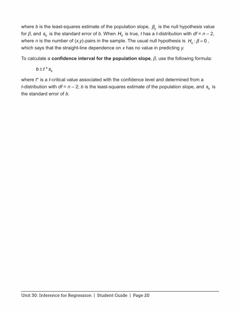
where b is the least-squares estimate of the population slope, β0 is the null hypothesis value for β, and bs is the standard error of b. When 0H is true, t has a t-distribution with df = n – 2, where n is the number of (x,y)-pairs in the sample. The usual null hypothesis is H0 :β = 0 , which says that the straight-line dependence on x has no value in predicting y.

To calculate a confidence interval for the population slope, β, use the following formula:

* bb t s±

where t* is a t-critical value associated with the confidence level and determined from a t-distribution with df = n – 2; b is the least-squares estimate of the population slope, and bs is the standard error of b.


The Video

Take out a piece of paper and be ready to write down the answers to these questions as you watch the video.

1. The population of peregrine falcons was in decline in the 1950s. What was the reason for the population’s decline?

2. In a scatterplot of eggshell thickness and log-concentration of DDE, which was the explanatory variable and which was the response variable?

3. Describe the form of the relationship between eggshell thickness and log-concentration of DDE – is the form linear or nonlinear? Positive or negative?

4. What is a population regression line?

5. Why are a and b, the y-intercept and slope of the least-squares line, called statistics?

6. State the null and alternative hypotheses used for testing whether the sample data provided strong evidence that higher levels of DDE were related to eggshell thinning in the population.


7. What was the outcome of the significance test?

8. Did the peregrine falcons ever recover?


Unit Activity: Clues to the Thief

A high school’s mascot is stolen and the poster shown in Figure 30.13 has been posted around the school and the town. The thief has left clues: a plain black sweater and a set of footprints under a window. The footprints appear to have been made by a man’s sneaker. Here are more details from the investigation:

• The distance between the footprints reveals that the thief’s steps are about 58 cm long. This distance was measured from the back of the heel on the first footprint to the back of the heel on the second.

• The thief’s forearm is between 26 and 27 cm. The forearm length was estimated from the sweater by measuring from the center of a worn spot on the elbow to the turn at the cuff.

Figure 30.13. The missing manatee.

School officials suspect that the thief is a student from a rival high school. Table 30.2 contains data from a random sample of 9th and 10th-grade students that you can use for this activity. Feel free to add and/or substitute data that your class collects.

In this activity, you will fit two linear regression models to the data. For the first model you will fit a line to forearm length and height; for the second model, you will fit a line to step length and height. To eliminate confusion, express your models using the variable names rather than x and y.


1. a. Make a scatterplot of height versus forearm length. Calculate the equation of the least-squares line and add its graph to your scatterplot.

b. Check to see if the four conditions for the simple linear regression model are reasonably satisfied. (Look to see if there are strong departures from the conditions.)

c. Calculate the standard error of the estimate, es .

2. Next, let’s focus on inference related to the relationship between height and forearm length.

a. We expect people with longer forearms to be taller than people with shorter forearms. Conduct a significance test H0 :β = 0 against Ha :β > 0 . Report the value of the test statistic, the degrees of freedom, the p-value, and your conclusion.

b. Construct a 95% confidence interval for β. Interpret your confidence interval in the context of this situation.

3. a. Make a scatterplot of height versus step length. Calculate the equation of the least-squares line and add its graph to your scatterplot.

b. Check to see if the four conditions for the simple linear regression model are reasonably satisfied. (Look to see if there are strong departures from the conditions.)

c. Calculate the standard error of the estimate, es .

4. Next, we focus on inference related to the relationship between height and step length.

a. We expect people with longer step lengths to be taller than people with shorter step lengths. Conduct a significance test H0 :β = 0 against Ha :β > 0 . Report the value of the test statistic, the degrees of freedom, the p-value, and your conclusion.

b. Construct a 95% confidence interval for β. Interpret your confidence interval in the context of this situation.

5. a. You have two competing models for predicting height, one based on forearm length and the other based on step length. Which of your two models is likely to produce more precise estimates? Explain.


b. Use one or both of your models to fill in the blanks in the following sentence. Justify your answer.

We predict that the thief is ______ cm tall. But the thief might be as short as ______ or as tall as ______.

Table 30.2. Data from 9th and 10-grade students.

Height Stride Length Forearm Length(cm) (cm) (cm)

Male 166.0 58.250 28.5Male 178.0 68.500 29.0Male 171.0 58.500 27.2Male 165.0 50.125 28.0Male 177.5 58.750 31.3Male 166.0 62.875 28.3Male 175.5 59.125 28.6Male 171.0 67.750 31.5Male 184.0 68.875 30.5Male 184.5 66.250 30.8Male 183.5 79.500 30.5Male 172.0 70.500 30.3

Female 164.5 55.875 24.2Female 166.0 52.375 27.3Female 168.0 55.375 28.0Female 178.5 59.750 29.1Female 166.0 48.375 27.9Female 159.0 57.125 28.0Female 166.0 64.000 27.4Female 154.5 57.750 25.8Female 161.0 63.500 27.0Female 177.0 69.750 30.1Female 161.0 72.500 26.5Female 164.0 75.250 28.2Female 174.0 58.500 28.4Female 164.0 59.750 26.8Female 168.0 55.250 26.4

Table 30.2

Gender


Exercises

Table 30.3 provides data on femur (thighbone) and ulna (forearm bone) lengths and height. These data are a random sample taken from the Forensic Anthropology Data Bank (FDB) at the University of Tennessee. Notice that height is given in centimeters and bone length in millimeters. All exercises will be based on these data.

Table 30.3. Data on femur and ulna length and height.

1. a. Make a scatterplot of height versus femur length. Would you describe the pattern of the dots as linear or nonlinear? Positive association or negative?

b. Calculate the equation of the least-squares line. Add a graph of the line to your scatterplot in (a).

c. Check to see if the conditions for regression inference are reasonably satisfied. Identify any strong departures from the conditions.

Femur Length, x1 Ulna Length, x2 Height, y(mm) (mm) (cm)432 237 158498 288 188463 276 173443 245 163511 278 191547 283 189484 279 178522 293 182438 251 163462 262 175449 255 159499 273 181484 280 168472 255 175484 269 175432 248 160439 248 165483 263 170484 269 180508 307 183

Table 30.3


2. a. Building on the work done for question 1, calculate the standard error of the estimate, es .

b. Write the equations of error bands one and two standard errors, es , above and below the least-squares line. Add graphs of these lines to your scatterplot from question 1(b).

c. If the distributions of the responses, y-values, for any fixed x are normally distributed with mean on the regression line, then the outermost bands in (b) should trap roughly 95% of the data between the bands. Is that the case?

3. a. Make a scatterplot of height versus ulna length. Determine the equation of the least-squares line and add a graph of the least-squares line to your scatterplot.

b. Calculate the standard error of the estimate, es .

c. Suppose a partial skeleton is found on a rugged hillside. The skeleton is brought to a lab for identification. The ulna bone measures 287 mm and the femur measures 520 mm. Use your equation from 3(a) to predict the person’s height. Then use your equation from 1(b) to predict the person’s height. Which of your estimates, the one based on ulna length or the one based on femur length, is likely to be more reliable? Justify your answer based on the standard error of the estimate, es , for each equation.

4. Consider the linear regression model for height based on femur length.

a. Test the hypothesis H0 :β = 0 against the one-sided alternative Ha :β > 0 . Report the value of the t-test statistic, the degrees of freedom, the p-value, and your conclusion.

b. Calculate a 95% confidence interval for the population slope, β.


Review Questions

1. The video focused on peregrine falcons and the relationship between eggshell thickness and log-concentration of DDE. During the video, we did not check whether or not the conditions for inference were met and went ahead with conducting a significance test and constructing a confidence interval. Your task is to check whether the four conditions for inference are reasonably satisfied given the following information. Justify your answer.

Assume that the data came from a random sample of eggs collected from Alaska and Northern Canada. Figure 30.14 shows a residual plot and Figure 30.15 displays a normal quantile plot of the residuals.

Figure 30.14. Residual plot.

Figure 30.15. Normal Quantile Plot of Residuals.

2.52.01.51.0

0.3

0.2

0.1

0.0

-0.1

-0.2

-0.3

Log-Concentration DDE

Resi

dual

s

Residual Plot

0.40.30.20.10.0-0.1-0.2-0.3-0.4-0.5

99.9

99

959080706050403020105

1

0.1

Residuals

Perc

ent

Normal Quantile Plot


2. Admissions offices of colleges and universities are interested in any information that can help them determine which students will be successful at their institution. For example, could students’ high school grade point averages (GPA) be useful in predicting their first-year college GPAs? Data on high school GPA and first-year college GPA from a random sample of 32 college students attending a state university is displayed in Table 30.4.

Table 30.4. Data on high school GPA and first-year college GPA.

a. Make a scatterplot of first-year college GPA versus high school GPA. Does the form of these data appear to be linear? Would you describe the relationship as positive or negative?

b. Determine the equation of the least-squares line and add the line to your scatterplot in (a).

c. Determine the t-test statistic for testing H0 :β = 0 . How many degrees of freedom does t have?

d. Find the p-value for the one-sided alternative Ha :β > 0 . What do you conclude?

3. Linda heats her house with natural gas. She wonders how her gas usage is related to how cold the weather is. Table 30.5 shows the average temperature (in degrees Fahrenheit) each month from September through May and the average amount of natural gas Linda’s house used (in hundreds of cubic feet) each day that month.

High School GPA First Year College GPA High School GPA First Year College GPA3.00 3.15 2.90 1.463.00 2.07 3.50 3.102.30 2.60 3.10 2.763.68 4.00 3.35 2.012.20 2.03 3.70 3.343.00 3.53 2.70 2.903.03 3.17 2.86 2.933.00 2.68 2.51 1.953.16 3.88 2.93 3.012.70 2.30 3.41 3.484.00 3.64 3.30 2.873.77 3.62 3.76 2.852.70 2.34 2.66 1.673.10 3.64 2.91 3.383.23 3.67 3.47 3.682.80 3.37 3.40 3.76

Table 30.4


Table 30.5. Gas usage and temperature data.

a. Make a scatterplot of gas usage versus temperature. Describe the form and direction of the relationship between these two variables.

b. Fit a least-squares line to gas usage versus temperature and add a graph of the line to your scatterplot in (a).

c. Check to see if the conditions needed for inference are satisfied.

d. Calculate the standard error of the estimate, es , and standard error of the slope, bs . Show your calculations.

e. Conduct a significance test of Ho :β = 0 . Should the alternative be one-sided or two-sided? Report the value of the t-test statistic, the degrees of freedom, the p-value and your conclusion.

f. Calculate a 95% confidence interval for the population slope. Interpret your results in the context of this problem.

4. Do taller 4-year-olds tend to become taller 6-year-olds? Can a linear regression model be used to predict a 4-year-old’s height when he or she turns six? Table 30.6 gives data on heights of children when they were four and then when they were six.

Table 30.6. Data on children’s heights at age 4 and 6.

Month Sep Oct Nov Dec Jan Feb Mar Apr MayOutdoor temperature °F 48 46 38 29 26 28 49 57 65Gas used per day (100 cu ft) 5.1 4.9 6 8.9 8.8 8.5 4.4 2.5 1.1

Table 30.5

Height Age 4 Height Age 6 Height Age 4 Height Age 6104.4 118.4 98.1 112.8104.0 119.4 100.6 115.292.1 103.9 100.5 115.8

103.3 116.8 102.7 117.398.4 113.1 98.5 113.396.5 110.0 98.8 109.3

105.3 119.3 102.3 117.9103.2 118.6 99.0 112.2105.9 123.2 100.2 112.997.4 110.2 100.3 113.4

103.4 118.7 99.6 112.6101.7 119.2 109.8 124.5105.4 120.2 100.2 113.7104.4 119.2 99.6 115.2100.7 112.6 104.1 117.1

Table 30.6


a. Make a scatterplot of height at age 6 versus height at age 4. Determine the equation of the least squares line and add its graph to the scatterplot.

b. From regression output we get 1.38596es = and 0.07437bs = . Construct a 95% confidence interval for the population slope β. Interpret your confidence interval in the context of children’s growth.

download unit 30 student guide

Documents