Download - © Copyright by Somdeep Chatterjee May 2016


© Copyright by
Somdeep Chatterjee
May 2016
_______________
A Dissertation
Presented to
The Faculty of the Department
of Economics
University of Houston
_______________
In Partial Fulfillment
Of the Requirements for the Degree of
Doctor of Philosophy
_______________
By
Somdeep Chatterjee
May, 2016
THREE ESSAYS ON ISSUES IN DEVELOPING ECONOMIES: CREDIT
REFORMS, ELECTIONS AND WAGE DISPERSION

THREE ESSAYS ON ISSUES IN DEVELOPING ECONOMIES: CREDIT
REFORMS, ELECTIONS AND WAGE DISPERSION
_________________________ Somdeep Chatterjee
APPROVED:
_________________________ Aimee Chin, Ph.D. Committee Co-Chair
_________________________ Gergely Ujhelyi, Ph.D.
Committee Co-Chair
_________________________ Chinhui Juhn, Ph.D.
_________________________ Francisco Cantú, Ph.D.
Department of Political Science University of Houston
_________________________ Steven G. Craig, Ph.D. Interim Dean, College of Liberal Arts and Social Sciences Department of Economics
ii

_______________
An Abstract of a Dissertation
Presented to
The Faculty of the Department
of Economics
University of Houston
_______________
In Partial Fulfillment
Of the Requirements for the Degree of
Doctor of Philosophy
_______________
By
Somdeep Chatterjee
May, 2016
THREE ESSAYS ON ISSUES IN DEVELOPING ECONOMIES: CREDIT
REFORMS, ELECTIONS AND WAGE DISPERSION

iv
Abstract
This dissertation presents three essays on some important issues in two develop-
ing economies, India and Ghana. In the first essay I analyze a major agricultural credit
reform in India, known as the Kisan Credit Card (KCC) scheme, which intended to
simplify the process of credit delivery in the agricultural sector. I use plausibly exoge-
nous variation in the reach of the program to find the causal effects of the policy on
agricultural output and technology adoption using a district panel data set. I also use
a household dataset to analyze the effects of differential exposure to this policy on a
wide range of household outcomes. I find evidence of increases in agricultural output
of rice, which is the major crop of the country. I also find that on average the use of
high yielding variety (HYV) seeds increases at the district level providing evidence
of technology adoption. The increase in output at the district level is corroborated by
suggestive increase in sales revenue and output of rice farmers at the household level.
In addition, I find evidence that bank borrowing increased for households due to this
program and the estimated effects on income and production are higher for such a
sub-sample of borrowers.
In the second essay, co-authored with Gergely Ujhelyi and Andrea Szabó, we try
to answer the question as to why people vote? One possibility is that they derive con-
sumption utility from doing so, but isolating this has proven empirically challenging.
In this paper we study a recent natural experiment in India, where legislative elections
have to provide a "None Of The Above" (NOTA) option to voters. Using the fact that
NOTA cannot affect the electoral outcome we show that studying individual voters’
behavior with and without NOTA provides a way to identify various components of
the consumption utility of voting. To address the challenge that individual votes are

v
not observable, we borrow techniques from the Industrial Organization literature to
estimate a structural model of voter demand for candidates and perform counterfac-
tual simulations removing the NOTA option. We complement this with a reduced-
form analysis of NOTA in a difference-in-differences framework, exploiting variation
in the timing of the reform created by the electoral calendar. Using both methods,
we find that NOTA increased turnout. We find minimal substitution between candi-
dates and NOTA, indicating that NOTA votes are cast by new voters who turn out
to vote specifically for this option. This indicates the presence of an option-specific
consumption utility of voting.
In the final essay, I use a matched employer-employee dataset from the Ghanaian
manufacturing sector to analyze earnings dispersion in Ghana from 1992-2003, a pe-
riod post extensive economic reforms. I find that variance of earnings increased from
1992-1998 and decreased thereafter resembling an inverted u-shaped relationship. I
use ANOVA and variance decomposition approaches to understand the underlying
factors that led to such a pattern in earnings inequality. I find that between-firm
factors explain this pattern more than within-firm factors. I also find that the mean
earnings gap between workers above and below the 90th percentile of income distri-
bution can explain majority of the initial surge in inequality (61%) but only explains a
very small fraction of the eventual decline (9%). I run modified Mincerian regressions
and decompose the variance components to find that the decline in earnings inequal-
ity is consistent with decline in variance of firm level earnings whereas variance of
predicted wage from worker characteristics have increased. I also find suggestive evi-
dence of changing patterns of worker-firm sorting which contributes to the decline in
inequality.

vi
Acknowledgements
The role of the Chair of the committee without doubt deserves the most plaudits
for a successful dissertation of a PhD student. I consider myself extremely lucky to
have had not one, but two people serve as co-Chairs of my committee. This not only
doubled my impetus towards achieving this target but also made me doubly more
determined to put my best foot forward towards producing this research output. As a
result I cannot thank Aimee Chin and Gergely Ujhelyi enough for acting as co-chairs
of my committee and guiding me at every step throughout my graduate student life
at the University of Houston. Professor Chin has truly been an academic mentor to
me from whom I could seek help for almost anything related to my career, not just my
research. Prof Ujhelyi on the other hand was the one who first encouraged me to start
thinking about research, right in my first year as a graduate student. The fact that I
started attending the Empirical Microeconomics seminar series every Tuesday right
from then is owed to him.
I must acknowledge the very important role played by the third member of my
dissertation committee, Chinhui Juhn. It was with her that I did my first independent
study in Grad school and the way she walked me through the papers we read together
and discussed every Friday will remain one of the most fruitful experiences of my life.
I must also take a moment to specially thank Janet Kohlhase for being super support-
ive during the lowest point of my days here at U of H. I also thank Bent Sørensen for
encouraging and uplifting me particularly at that time and for being a great Grad Di-
rector to all of us in general. I thank Amber Pozo for her great administrative support
throughout my career at University of Houston.

vii
I would also like to thank Andrew Zuppann for his comments and suggestions
at various times and for giving the chance to present preliminary work in the Brown
Bag sessions and thank all the attendees. I have benefitted greatly from all of their
comments which I will perhaps miss the most, apart from the delicious food! I thank
all the other faculty members of the department of Economics for providing feedback
at various times during seminars. I would be failing in my duty if I do not specially
mention Andrea Szabó for being an amazing co-author. I am grateful to Francisco
Cantú from the Department of Political Science for being the external member of my
dissertation committee. Life at UH would not have been as great had it not been
for my fantastic classmates and colleagues. I thank Chon-Kit for the many useful
discussions. I thank Bocong for being such a great friend and confidante and Subash
for being extremely supportive. For the innumerable memories at UH, within and
outside the department, I must thank Gautham, Vinh, Max, Xuejing, Shoumen, Aritri,
Indrajit, Debashis and so on but I apologize to everyone whose names I cannot take
due to paucity of space.
While one is at grad school, he requires a solid support system from outside and
back home. I was lucky to have one. I cannot express in words the contribution of my
parents, Srabani and Somnath. Everything that I am today is due to them and there
are no other contenders befitting for me to dedicate this thesis to. I must thank my
professors from my alma mater in India, Ajitava Raychaudhuri, Saikat Sinha Ray and
Swapnendu Banerjee for believing in me, my greatest buddy and childhood friend
Sayantan for being there at all times, my closest friend from college Saumik for being
who he is.
Last but in no way the least, I was blessed to have unbelievable grandparents for

viii
super important emotional support and much needed pampering at times. The con-
tribution of Dadai, Chotdadu and Monididi cannot be quantified here. Even though
Mammam could not live to see this day, I am sure she has always been with me from
wherever she is now and would have been the happiest person on earth today.

ix
Contents
1 Effects of Agricultural Credit Reforms on Farming Outcomes: Evidence from
the Kisan Credit Card Program in India. 1
1.1 Introduction . . . . . . . . . . . . . . . . . . . . . . . . . . . . . . . . . . . 1
1.2 Background . . . . . . . . . . . . . . . . . . . . . . . . . . . . . . . . . . . 6
1.2.1 The Kisan Credit Card Program . . . . . . . . . . . . . . . . . . . 6
1.2.2 Conceptual Framework and Related Literature . . . . . . . . . . . 9
1.3 Empirical Strategy . . . . . . . . . . . . . . . . . . . . . . . . . . . . . . . 12
1.4 Data . . . . . . . . . . . . . . . . . . . . . . . . . . . . . . . . . . . . . . . . 17
1.5 Results . . . . . . . . . . . . . . . . . . . . . . . . . . . . . . . . . . . . . . 21
1.5.1 Results using District-Panel Dataset . . . . . . . . . . . . . . . . . 21
Effects on Crop Production . . . . . . . . . . . . . . . . . . . . . . 21
Technology Adoption . . . . . . . . . . . . . . . . . . . . . . . . . 22
Threats to Identification: Check for Pre-Trends . . . . . . . . . . . 23
1.5.2 Do Households Change their Borrowing Patterns? . . . . . . . . . 24
Total Borrowing . . . . . . . . . . . . . . . . . . . . . . . . . . . . . 25
Analysis of the Largest Loans . . . . . . . . . . . . . . . . . . . . . 26
1.5.3 Effects on Household Production, Income and Consumption . . . 27
Rice Production and Sales . . . . . . . . . . . . . . . . . . . . . . . 27
Income . . . . . . . . . . . . . . . . . . . . . . . . . . . . . . . . . . 28

x
Consumption Expenditures . . . . . . . . . . . . . . . . . . . . . . 29
1.5.4 Falsification Exercise . . . . . . . . . . . . . . . . . . . . . . . . . . 30
1.6 Conclusions . . . . . . . . . . . . . . . . . . . . . . . . . . . . . . . . . . . 31
1.7 References . . . . . . . . . . . . . . . . . . . . . . . . . . . . . . . . . . . . 33
2 “None of the Above" Votes in India and the Consumption Utility of Voting
(with Gergely Ujhelyi and Andrea Szabó) 46
2.1 Introduction . . . . . . . . . . . . . . . . . . . . . . . . . . . . . . . . . . . 46
2.2 The consumption utility of voting . . . . . . . . . . . . . . . . . . . . . . . 51
2.3 Background . . . . . . . . . . . . . . . . . . . . . . . . . . . . . . . . . . . 55
2.3.1 The Indian NOTA policy . . . . . . . . . . . . . . . . . . . . . . . . 55
2.3.2 NOTA-like options in other countries . . . . . . . . . . . . . . . . 56
2.3.3 Assembly elections in India . . . . . . . . . . . . . . . . . . . . . . 58
2.4 Data . . . . . . . . . . . . . . . . . . . . . . . . . . . . . . . . . . . . . . . . 61
2.4.1 Samples used for analysis . . . . . . . . . . . . . . . . . . . . . . . 61
2.4.2 Election data . . . . . . . . . . . . . . . . . . . . . . . . . . . . . . 62
2.4.3 Voter demographics . . . . . . . . . . . . . . . . . . . . . . . . . . 63
2.5 Patterns in the data . . . . . . . . . . . . . . . . . . . . . . . . . . . . . . . 65
2.5.1 NOTA votes . . . . . . . . . . . . . . . . . . . . . . . . . . . . . . . 65
2.5.2 The effect of NOTA on turnout . . . . . . . . . . . . . . . . . . . . 67
2.6 Estimating the effect of NOTA from a demand system for candidates . . 70
2.6.1 Specification: demand . . . . . . . . . . . . . . . . . . . . . . . . . 71
2.6.2 Specification: supply . . . . . . . . . . . . . . . . . . . . . . . . . . 74
2.6.3 Estimation . . . . . . . . . . . . . . . . . . . . . . . . . . . . . . . . 77
2.6.4 Practical issues . . . . . . . . . . . . . . . . . . . . . . . . . . . . . 80

xi
2.6.5 Results . . . . . . . . . . . . . . . . . . . . . . . . . . . . . . . . . . 81
Parameter estimates . . . . . . . . . . . . . . . . . . . . . . . . . . 81
Counterfactual analysis: The impact of NOTA . . . . . . . . . . . 82
2.7 Conclusion . . . . . . . . . . . . . . . . . . . . . . . . . . . . . . . . . . . . 84
2.8 References . . . . . . . . . . . . . . . . . . . . . . . . . . . . . . . . . . . . 85
2.9 Appendix . . . . . . . . . . . . . . . . . . . . . . . . . . . . . . . . . . . . 90
2.9.1 The correlates of NOTA votes . . . . . . . . . . . . . . . . . . . . . 90
2.9.2 Robustness of the DD estimates . . . . . . . . . . . . . . . . . . . . 91
National elections . . . . . . . . . . . . . . . . . . . . . . . . . . . . 91
Redistricting . . . . . . . . . . . . . . . . . . . . . . . . . . . . . . . 92
State-specific events . . . . . . . . . . . . . . . . . . . . . . . . . . 93
3 Firm Ownership and Wage Dispersion: Evidence from Ghana Using Matched
Employer Employee Data 110
3.1 Introduction . . . . . . . . . . . . . . . . . . . . . . . . . . . . . . . . . . . 110
3.2 Background . . . . . . . . . . . . . . . . . . . . . . . . . . . . . . . . . . . 113
3.2.1 The Ghanaian Manufacturing Sector . . . . . . . . . . . . . . . . . 113
3.2.2 Related Literature and Conceptual Framework . . . . . . . . . . . 115
3.3 Empirical Methodology . . . . . . . . . . . . . . . . . . . . . . . . . . . . 116
3.3.1 Analyis of Variance . . . . . . . . . . . . . . . . . . . . . . . . . . . 116
3.3.2 Percentile Analysis: Contribution of Earnings Gap to Variance . . 117
3.3.3 Worker Characteristics and Firm Fixed Effects . . . . . . . . . . . 117
3.4 Data . . . . . . . . . . . . . . . . . . . . . . . . . . . . . . . . . . . . . . . . 118
3.5 Results . . . . . . . . . . . . . . . . . . . . . . . . . . . . . . . . . . . . . . 120
3.5.1 Within-Firm and Between-Firm Effects . . . . . . . . . . . . . . . 120

xii
3.5.2 Percentile Analysis . . . . . . . . . . . . . . . . . . . . . . . . . . . 122
3.5.3 Returns to Schooling and Earnings Dispersion . . . . . . . . . . . 124
3.5.4 Does Predicted Wage Dispersion by Worker and Firm Charac-
teristics Vary by Ownership Structure? . . . . . . . . . . . . . . . 124
3.6 Conclusions . . . . . . . . . . . . . . . . . . . . . . . . . . . . . . . . . . . 126
3.7 References . . . . . . . . . . . . . . . . . . . . . . . . . . . . . . . . . . . . 127

xiii
List of Figures
1.1 Crop Production: Year-specific coefficients for aligneds ·morebanksd . . 38
1.2 HYV Use: Year-specific coefficients for aligneds ·morebanksd . . . . . . . 39
2.1 Constituencies in the merged dataset . . . . . . . . . . . . . . . . . . . . . 102
2.2 Distribution of NOTA vote shares across constituencies . . . . . . . . . . 107
2.3 Impact of NOTA on turnout . . . . . . . . . . . . . . . . . . . . . . . . . . 108
2.4 Impact of NOTA on candidates’ vote shares . . . . . . . . . . . . . . . . . 109
3.1 Share of Firms by Ownership Type . . . . . . . . . . . . . . . . . . . . . . 129
3.2 Time Series Plots of Firm Averages by Ownership Types: Firm Dataset
of 200 Firms over 12 Years . . . . . . . . . . . . . . . . . . . . . . . . . . . 135
3.3 Variances of Log Real Hourly Earnings by Ownership Type . . . . . . . . 136

xiv
List of Tables
1.1 Comparing Means of statewise spread of KCC in 2000 by aligned . . . . 37
1.2 VDSA District Dataset: Effects on Crop Production and HYV Use . . . . 40
1.3 IHDS Dataset: Effects on Borrowing Composition . . . . . . . . . . . . . 41
1.4 IHDS Dataset: Effects on Rice Production and Sales . . . . . . . . . . . . 42
1.5 IHDS Dataset: Effects on Income . . . . . . . . . . . . . . . . . . . . . . . 43
1.6 IHDS Dataset: Effects on Consumption Expenditure . . . . . . . . . . . . 44
1.7 Falsification Exercise . . . . . . . . . . . . . . . . . . . . . . . . . . . . . . 45
2.1 Timeline of events in the study period . . . . . . . . . . . . . . . . . . . . 95
2.2 Summary statistics of the electoral data at the constituency level . . . . . 96
2.3 Candidate characteristics in the panel data . . . . . . . . . . . . . . . . . 97
2.4 Voter demographics at the state level (repeated cross-section) . . . . . . . 97
2.5 Demographic characteristics of the constituencies from the Indian Cen-
sus (panel dataset) . . . . . . . . . . . . . . . . . . . . . . . . . . . . . . . 98
2.6 The impact of NOTA on turnout, DD estimates . . . . . . . . . . . . . . . 99
2.7 Estimates of the linear parameters of the demand system . . . . . . . . . 100
2.8 Estimates of the nonlinear parameters of the full model . . . . . . . . . . 101
2.9 Impact of NOTA on vote shares by party . . . . . . . . . . . . . . . . . . 103
2.10 The correlates of NOTA votes . . . . . . . . . . . . . . . . . . . . . . . . . 104

xv
2.11 Effect of NOTA on turnout, excluding national election years . . . . . . . 105
2.12 Effect of NOTA on turnout, controlling for redistricting . . . . . . . . . . 105
2.13 Effect of NOTA on turnout, robustness to state-specific events . . . . . . 106
3.1 Descriptive Statistics . . . . . . . . . . . . . . . . . . . . . . . . . . . . . . 130
3.2 Analysis of Variances of Log Real Hourly Earnings of Workers . . . . . . 131
3.3 Variances of Log Real Hourly Earnings of Workers by Ownership Type . 131
3.4 Contribution of Earnings Gap to Variance in Earnings . . . . . . . . . . . 132
3.5 Returns to Schooling and Experience . . . . . . . . . . . . . . . . . . . . . 133
3.6 Variance Decomposition: Estimated Firm Effects and Predicted Wage
from Worker Characteristics . . . . . . . . . . . . . . . . . . . . . . . . . . 134

xvi
To Baba and Ma...for everything and more!!!

1
Chapter 1
Effects of Agricultural Credit Reforms
on Farming Outcomes: Evidence from
the Kisan Credit Card Program in India.
1.1 Introduction
Providing access to financial resources to the poor continues to be an important pol-
icy prescription in the literature even though the empirical evidence on impacts of
credit constraint relaxations and expansion of credit options for the unconstrained in
developing countries is mixed (Karlan and Murdoch 2009). To design effective poli-
cies that provide or expand access to credit, one would first need to understand the
mechanisms through which credit access helps the poor and also the impact of im-
plementing such a policy on the targeted beneficiaries. To estimate these impacts, the
ideal experiment would be to randomly provide credit products to households and
compare the outcomes of the ones getting access to the ones without access to this
product. The January 2015 issue of AEJ Applied has six papers on this subject using

randomized evaluations.1 These papers find little to no impact of providing access to
finance. Other papers like de Mel, Mckenzie and Woodruff (2008) using experimental
designs find positive impacts.
While randomized evaluations are ideal to identify the causal effects of credit con-
straint relaxations, by design these cater to a relatively small sample of the entire pop-
ulation. Whether a large scale national reform would replicate these findings is impor-
tant to understand. In this paper, I look at a major overhaul in the agricultural credit
delivery process in India in 1998, known as the Kisan Credit Card (KCC) program,
and evaluate the impacts of this policy. The targeted group for this credit reform was
rural agricultural households, generally involved in farming and other related occu-
pations. Ease of delivering agricultural credit, reasonable interest rates and relaxation
of monitoring norms were the key features of this program. Reports from the Planning
Comission of India (2002) suggest that by 2000-01, KCCs constituted almost 71% of the
total production credit disbursement by commercial banks. It was also the dominant
mode of production credit delivery for other banks. The report also suggests that in
the first two years, close to 4 million credit cards were issued with a total disbursal of
credit lines worth 50 bllion INR (1 billion USD approximately).
Although this was a major policy reform, to date there has been little convincing
evidence of the impacts of this program. Chanda (2012) uses post-policy state level
data from 2004-2009 to see if growth in KCC issues lines up with increases in agri-
cultural productivity. There are other government of India commissioned descriptive
reports like the Planning Commission report mentioned above and Samantara (2010).
In this paper, I use a country wide district panel dataset to evaluate the causal effects
1All the 6 papers are cited in the references.
2

of this program on agricultural output and technology adoption. I also use household
data to estimate the impacts of this program on a wide range of outcomes including
income, consumption and borrowing.
The reach of formal financial institutions is not universal in most developing coun-
tries. This is because banks would want to select into richer regions unless they are
administratively required to setup branches in unbanked locations. This makes for-
mal credit markets less accessible to the poor in these areas. The KCC reform therefore
provides an opportunity to add to this literature of how access to formal credit insti-
tutions can help the poor sections of the society in line with Burgess and Pande (2005).
The unique feature of the KCC program was that it catered exclusively to the agricul-
tural sector. Although in this paper, I am not able to distinguish whether the effects
of KCC operate through channels of new access to credit or expansion of credit to the
ones who already had some access. As a result most of my estimations should be
viewed as a bundle of reduced form effects.
This paper takes advantage of rules in implementation of the policy to generate
plausibly exogenous variation in access to this program to identify causal effects of
the reform. The identification strategy relies on variation across three main dimen-
sions. First is the time dimension. The policy was implemented in 1998 and I look at
the outcomes in years before and after the policy. Second, is the political alignment di-
mension, ie, whether the state government is ruled by a party aligned with the central
government in the federal structure of India. Political alignment has been widely re-
garded to be important for policy implementation and performance (see Chibber et al
2004, Iyer and Mani 2012 and Asher and Novosad 2015). The final source of variation
comes from how the rolling out of these credit cards was implemented. The KCCs
3

could only be issued through formal banks and not by any other agency. I use district
level variation in the number of bank branches already setup prior to the policy to
proxy for access to this program.
I propose to identify the causal effect of the policy by the interaction of these three
variables. The effect is identified by looking at the difference in outcomes after and
before the policy in districts with more bank branches over districts with fewer bank
branches in states that are ruled by political parties aligned with the central govern-
ment after controlling for these differences in districts in the states not aligned with
the center. I use pre-policy data to show that these regions were not already different
along the relevant dimensions to provide support to the identifying assumption that
any differences post-policy are attributable to the program.
I find that increased access leads to significantly higher production levels. Rice is
the major crop of India and I find an aggregate increase in production by 88 thousand
tonnes (metric ton) per year on average which is between 1/3 to 1/4 of an increase
compared to the mean. 2 Corresponding to this large change, I find that technology
adoption has also been significant. Crop production area under high yielding variety
(HYV) seeds increased by around 71 thousand hectares at an aggregate level which
is just under a 1/3 increase compared to the mean. This suggests that with increased
access to credit, districts exposed to the program fared significantly better in terms
of porduction and technology adoption. Using houseold data, I corroborate some of
these results. I find suggestive evidence of increases in rice production for farmers
even though estimated imprecisely. I am constrained by the fact that the household
2The Food and Agricultural Organization’s FAOSTAT indicates that in 2012, the value of rice pro-duced in India is over 40 billion US dollars which makes it the most valuable crop of India. Rice hasconsistently been the major crop of India in terms of overall value for years. See - faostat.fao.org
4
data comes only from a sample of farmers and not the universe, unlike the district
panel data described above which contains all rice production in the districts. I find
that revenue from sales of rice is higher for farmers potentially exposed to KCC.
The advantage of using household data is being able to observe borrowing pat-
terns. Using a cross-section of households, I find that households are more likely to
have fewer but larger loans with exposure to KCC. I also find that they are more likely
to have larger bank loan sizes if exposed to KCC. These effects seem to be larger for
those households which report cultivation as their main source of income and for rice
farmers. This is reassuring because most of the production effects observed using the
district data seem to suggest that rice farmers would be most affected by this policy.
I find that even though on average there is no effect on income but farm income
is higher by 129 Indian rupees (USD 2) per month for households whose main in-
come source was cultivation. Compared to the mean, the magnitude of this effect is
almost 25%. This is consistent with the findings on production and sales. With higher
sales, we might expect higher profits, ceteris paribus. I find no overall impacts on con-
sumption expenditure but composition of consumption changes. I find higher daily
expenditures but lower expenditure on consumption like tobacco and beetel leaves.
I do not find any effects on the margin of whether a household is likelier to have a
bank loan in response to the policy. Since I do find that households have a higher bank
loan size conditional on borrowing, this allows me to analyze a sub sample of house-
holds seperately. I look at all the outcomes for only those households who borrow
from banks and I find that all the effects described above are much more pronounced
for this group. Since KCC had to operate through banks, this gives us confidence that
our estimated effects are likely to be mediated through bank borrowing which should
5

include KCC borrowing.
The rest of the paper is organized as follows. Section 2 provides background infor-
mation. Section 3 describes the empirical strategy. Section 4 explains the Data. Section
5 presents results and Section 6 concludes.
1.2 Background
1.2.1 The Kisan Credit Card Program
Agriculture constitues roughly a fifth of the total GDP of India and employs two out
of three Indian workers. In the late nineties, agriculture started opening up to the mar-
ket rather than being limited to subsistence farming. Agricultural credit has played an
important role in developing the market for such produce and help improve the con-
dition of farmers in the country. However, the finance and credit institutions present
in the country prior to 1998 were deemed inefficient by several reports and experts and
as a result the Kisan Credit Card program was envisaged. This scheme was launched
in 1998 and was introduced for the first time in the budget speech of the Finance Min-
ister of India in the parliament. Within a year after its inception around 5 million cards
were issued to farmers. Prior to 1998, the system of agricultural credit delivery was
complicated. A multi agency approach was used where borrowers had to go through
several layers of bureaucracies depending on the purpose of their loans (Samantara
2010). KCC also brought about a revolving credit regime as opposed to the existing
demand loan system (Chanda 2012).
At its inception, the KCC was not a traditional credit card that is commonly used.
The card was a mere documentation for identifying the individual and his credit line
6

with a given bank. It did not have features that allowed payments at merchant outlets.
This also makes the presence of banks an important dimension for identifying the
intensity of reach of the program. The way to use a KCC was to visit the bank branch
in person and withdraw a certain amount of money which could then be used for
purchases. This also ruled out the possibility of banks monitoring the usage of the
loans.
The most important feature of this credit product was the ease of availability of
loan. Some banks laid down rules for eligibility like having title to an acre of irrigated
land. On fulfiling this criterion, the farmer would be eligible for a loan with a bank
without any collateral requirement for an amount upto 50,000 INR (around 1000 USD
back then). The KCC accounts were largely valid for 3 years and repayment time
frames spanned upto a year. On successful replayments and responsible credit use,
these accounts were renewable but the initial approval was given largely without any
bacground checks. As pointed out above, a big difference from existing crop loans
was that the usage of the KCC loans were not monitored whereas most agro-credit
was tied to agricultural use or purchase of inputs, fertilizers etc. So, a farmer could
get a KCC account and use the amount for personal consumption.
In a way KCC provided the best available source of personal credit to poor farmers.
The biggest advantage over microfinance institutions were that KCC was operational
through formal banks and charged a very reasonable interest rate of around 7% per
annum as opposed to as large as 36-40% rates charged by self help group microcredit
institutions. The approval process was also very simple and was a single window
exercise as the only criterion was ownership of an acre of irrigated land. Many banks
have recorded allowance of credit limits in excess of 50,000 INR but in such cases
7

they often asked for collaterals. Therefore larger scale farmers who are financially in
a better off situation were only likely to go for these loans. There was no clause to my
knowledge which restricted large farmers from opening a KCC account.
Samantara (2010) points out that a major reason why KCC was launched was to
integrate the various credit needs of farmers, from personal consumption to festival
expenditure, education, health and agricultural needs, into one comprehensive prod-
uct. Earlier a farmer had to weigh multiple options based on the purpose of his loan.
KCC made it a one stop procedure wherein he could withdraw the requisite amount
and use it for any purpose whatsoever. All the bank cared about was the timely re-
payment and not the usage. This was a major shift from the pre-existing agro-credit
policy in India which was called the Agricultural Credit Delivery System. Under that
system, a multi-product multi-agency approach was adopted. Policy makers in the
country had planned this in a way such that specific needs of farmers could be ad-
dressed by specific credit products. A farmer could go to a bank for purchase of a
particular input and get a loan against that purchase. The idea was more like financ-
ing purchases rather than giving out cash loans. From such a scheme KCC came as
a welcome change which sought to replace the multi-product approach in favor of
a cash credit approach in a single comprehensive product. As might be already evi-
dent from this discussion, KCC was intended to address the short term credit needs of
farmers and not the longer term needs. Since there was no monitoring, one could not
rule out the possibility of withdrawing cash from these accounts and using them for
consumption purposes. At present, Kisan Credit Cards are available as differentiated
products with various banks coming out with various varieties and features.
Overall the Kisan Credit Card program should be viewed as a bundle of reforms in
8

one. It not only aimed to relax credit constraints by making loans available to the ones
constrained prior to 1998 but also provided a source of flexible credit. KCCs could
potentially finance a lot of purchases, not just agricultural inputs and therefore have
wider social consequences. Since KCCs were a source of cheaper credit, one might
also view it as expansion of credit options for the ones already having access to other
forms of credit. Unconstrained farmers may now be attracted to borrow at cheaper
rates and finance their short term credit needs.
1.2.2 Conceptual Framework and Related Literature
To estimate the true causal effects of access to credit one would ideally want to gen-
erate random variation in access to financial institutions. There is a rich literature
comprising of experimental studies along these lines (Angelucci, Karlan and Zinman
2015, Attanasio et al 2015, de Mel, Mckenzie and Woodruff 2008, Augsburg et al 2015,
Banerjee et al 2015, Crepon et al 2015, Tarozzi, Desai and Johnson 2015). Apart from
this there is a quasi-experimental literature which looks at policy reforms in the formal
financial sector to answer a similar question (Burgess and Pande 2005, Banerjee and
Duflo 2014). Government policy reforms are usually not randomly assigned, there-
fore identifying the causal effects of such programs is challenging even though it is
important to understand the mechanisms behind such policies aimed at removal of
borrowing constraints.
Most recent studies on the role of credit access focus largely on this aspect of mech-
anisms of credit delivery (Karlan and Morduch 2009). This paper is the first to objec-
tively evaluate the Kisan Credit Card scheme using a district panel dataset and ex-
tends this literature by looking at this large scale national reform in credit delivery
9

mechanism. In the Indian context, Banerjee and Munshi (2004) and Banerjee and Du-
flo (2014) study the role of credit constraints on firms and businesses. However the
role of credit constraints in agricultural occupations has been little studied till date.
This paper also contributes to the literature by attemtping to fill this void.
An important question that arises here is whether this program should be viewed
as enhanced ‘access’ to agricultural credit or ‘expansion’ of credit to the ones who al-
ready had access to credit? The existence of credit constraints and impediments to
borrowing are major roadblocks in developing economies which is why governments
may want to innovate by reforming the system of credit delivery. If the main objec-
tive is to improve the condition of the poor, one would imagine that removing the
borrowing constraints would be important, or in other words a program like KCC
should have given ‘access’ to credit to the ones who never had the chance to borrow
before. The starting point of the analysis is to understand how we expect credit access
to affect the credit constrained? If KCC relaxed credit constraints and people unable
to borrow elsewhere could now borrow under this program, economic theory and
existing empirical evidence would lead us to expect multiple effects.
First, if households invest in productive assets or the borrowed funds are used to
finance improvements in technology of agricultural production, we expect their agri-
cultural income to be higher. Second, if we aggregate these effects, overall production
of crops should be higher and overall adoption of new technology should also be
higher. Third, composition of consumption may change. Banerjee et al (2015) find
such evidence in a microfinance experiment but the idea is applicable to a broader
10

country wide setting as well because in essence we are thinking of the impact of relax-
ation of credit constraints per se. Finally, since this was a national level formal lend-
ing program, one would expect that with enhanced access informal lending would go
down and be substituted by more formal sector loans.
The flip side however, is that from a lender’s perspective, such a policy may at-
tract poor quality borrowers. This leads to issues of adverse selection. Asubel (1991)
discusses credit card markets in the US and how lowering interest rates are far from
ideal from a bank’s perspective as bad borrowers may select into borrowing at lower
rates. KCC lending was usually at a much lower rate of interest than market rates or
informal lending rates prevalent among microfinance institutions. This would have
meant that the adverse selection issue was likely to be severe under this program.
Also since new borrowers are unlikely to have ever engaged in credit dealings, their
perception about their own future stream of income determining their repaying abil-
ity is likely to be myopic. Melzer (2011) and Bond, Musto and Yilmaz (2009) point
out these problems about ‘misinformed’ borrowers underestimating their future re-
payment commitments.
It is also important to think about potential general equilibrium effects of this pro-
gram. Are there any spillovers? For example, if some farmers get credit cards whereas
others do not, maybe they have a competitive advantage over the ones who did not get
this card and this might lead to perverse welfare implications. Similarly, if KCCs are
very attractive and result in high profits for farmers, this maybe an incentive for non-
farmers to take up agricultural occupations which in turn may affect non-agricultural
sectors in the rural areas.
11

1.3 Empirical Strategy
There are two parts in my empirical strategy. I have the twin objective of evaluating
the overall effects of access to credit on production outcomes on average and also
whether access to credit through such a reform is useful for intended beneficiaries.
To this end, I use two different datasets. The first is a district panel dataset and the
second is a cross-sectional household dataset.
Identifying the causal effects of having a KCC on agricultural outcomes using sur-
vey data is difficult because KCCs were not randomly assigned to households. Also,
using a cross sectional dataset, it is not possible to use time varying access to the
scheme either. 3 To overcome these issues, I propose an identification strategy that re-
lies on plausible exogenous variation in the reach of this program to find causal effects
of the program. Apart from the time dimension (program introduced in 1998) which
provides variation in the access to the program over the span of the data, there are two
different cross sectional dimensions that give us a sense of which regions might have
had more access to these cards after the policy. I use an interaction of these dimesions
to identify effect of the policy.
The KCC program was announced by the Finance Minister of India in his budget
speech in 1998 and the implementation began soon after. The government at the cen-
ter was ruled by the Bharatiya Janata Party (BJP) led National Democratic Alliance
(NDA) coalition. However, not all state governments were run by the NDA coalition.
Since the implementation of this policy required a lot of work at the grass roots in
terms of setting up infrastructure, spreading awareness, nudging banks to implement
3Even though there is no clear idea even in government documents in terms of how these cards wererolled out.
12

this policy and the like, one can understand that the role that state governments and
officials at the village and block levels who are employed by the state governments
would have had an important role to play in the penetration of this policy in those
states. This gives one potential source of variation in the policy. I use an indicator
variable aligned which takes the value 1 if the state in question was ruled by the BJP
or one of its NDA allies in 1998 and 0 otherwise. The idea is that aligned states would
probably have earlier or quicker access to this policy whereas the opposition parties
may choose to be slack in the policy implementation in the states where they are in
power, out of several motives including the fact that they would want the scheme to
be projected as a failure for the ruling coalition and take advantage of this in future
elections themselves.
The first real governmental study on the program outreach was done in 2002 by the
Planning Commission of India. They published a report with tables on the state wise
coverage of Kisan Credit Cards as of March 2000, which is 2 years into the program.
The coverage rates were basically the number of KCCs issued by various banks as a
percentage of total operational land holdings in the concerned state. So this gave an
idea as to how many farmers were potentially reached or covered under the policy
within the first two years of the policy at a state level. If we observe that aligned states
actually were implementing the policy faster than the other states, we might be more
confident about the use of this dimension to identify the effects of the program. Table
1.1 provides supportive evidence. I find that coverage in aligned states is almost 2.5
times the coverage in rest of the states and the difference is statistically significant at
the 99% level of confidence.
13
The second dimension that I bring to this analysis of variation in access is a techni-
cality that the policy had. These credit cards could only be given out through banks.
So it is understandable that areas with more banks are likely to be able to roll out these
cards faster than the ones which are unbanked or have fewer banks. However, there
may be concerns that banks opened up or positioned or repositioned themselves based
on the policy announcement in markets where KCC lending would flourish more. To
account for this issue I use bank data at the baseline year, ie, 1998 and not after the
policy. I use district level existing bank branches data from 1998 to enumerate the
number of branch offices of banks at the time of announcement of the policy. This
gives us another potential exogenous source of variation in the intensity of coverage
of the program. I create the variable bank98 to denote the number of bank branches
in a given district in 1998 and use the indicator variable morebanks which takes the
value 1 for districts with number of banks above the mean of bank98.
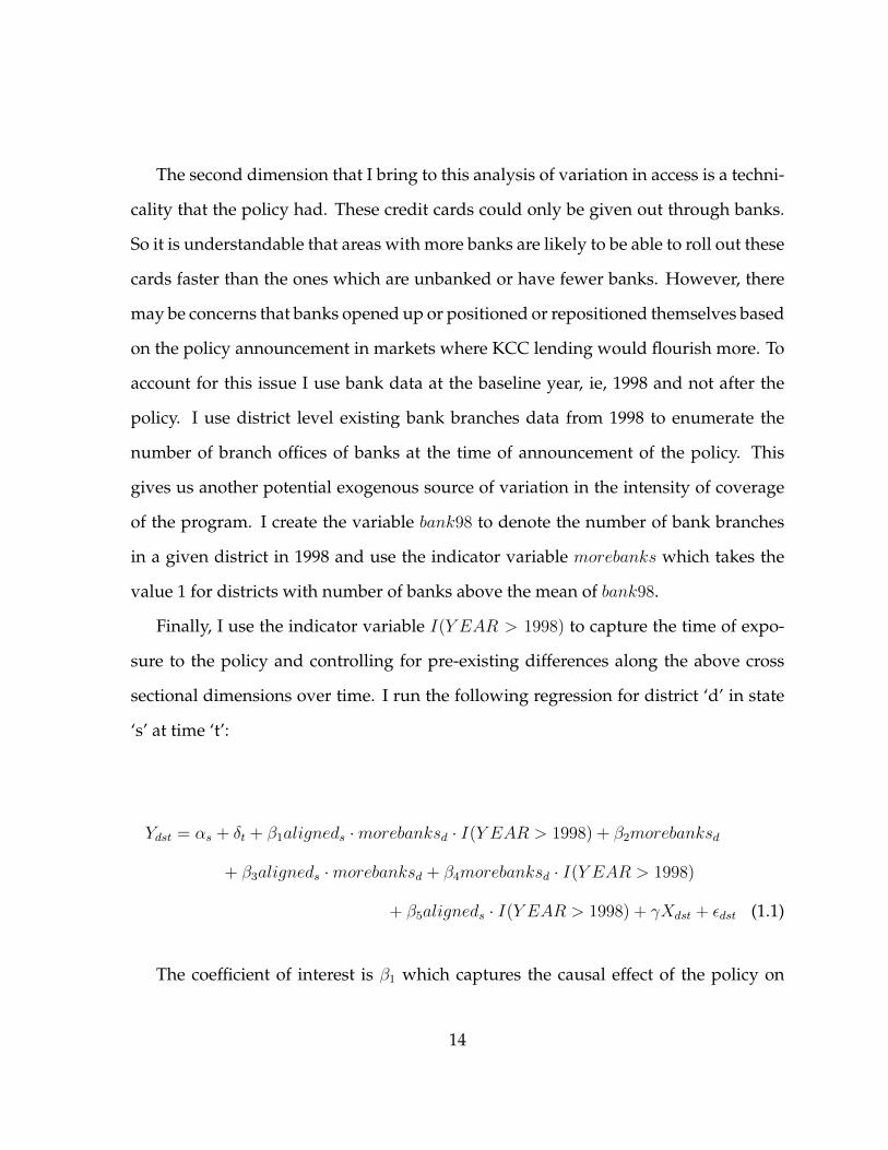
Finally, I use the indicator variable I(Y EAR > 1998) to capture the time of expo-
sure to the policy and controlling for pre-existing differences along the above cross
sectional dimensions over time. I run the following regression for district ‘d’ in state
‘s’ at time ‘t’:
Ydst = αs + δt + β1aligneds ·morebanksd · I(Y EAR > 1998) + β2morebanksd
+ β3aligneds ·morebanksd + β4morebanksd · I(Y EAR > 1998)
+ β5aligneds · I(Y EAR > 1998) + γXdst + εdst (1.1)
The coefficient of interest is β1 which captures the causal effect of the policy on
14

outcomes Y . I use state fixed effects captured by αs. Demographic controls at the
household level are included in X . I control for the number of persons in the fam-
ily, number of children, number of married men and women and also the age and
education levels of men and women.
The interpretation of β1 is that it gives us the difference over time (post- and pre-
policy) in Y for households in districts with more banks compared to households
in districts with lesser banks in aligned states after controlling for these same differ-
ences in non-aligned states. The identifying assumption is that the outcome Y would
not have been different for these groups of households had there been no KCC pol-
icy. There is no standard way to validate this assumption and identification always
assumes this, but the panel structure of the data provides an opportunity to check
whether these districts were historically different and already had differential trends
even before the policy. If we find that before the policy, differences in outcomes along
the above dimensions were not different, we gain confidence that the identifying as-
sumption is plausible. I describe a check for this at a later section and find that before
1998 there were indeed no differences in outcomes in these areas.
The fact that prior to the policy, the cross sectional dimensions seem to be similar,
leads us into the cross sectional analysis. The dataset that I use is from 2005 which is a
post-policy year. I still use the above cross sectional dimensions to generate exogenous
variation in access to the policy but do not have the time dimensions anymore. Since
there were no differences in these regions prior to the policy, any difference that I find
for 2005 can be attributed as a causal effect of the program.
Using the household dataset, I therefore propose to run the following regression
for household h in district d and state s:
15

Yhds = αs + θ1(aligned ·morebanks)ds + θ2(morebanks)d + ωXhds + uhds (1.2)
In this specification, θ1 is the causal impact of the policy on outcomes Y . The
identifying assumption here, similar to above, is that in the absence of the policy,
the differences in household outcomes between districts with more and less banks in
aligned states would not have been any different from the differences in household
outcomes in more and less bank districts in non-aligned states.
The main outcome that I look at is crop production. As mentioned earlier, rice is
the major crop of the country in terms of value. I focus primarily on rice production
but also look at the other important crops like wheat and maize. The idea is that
with access to credit, farmers may be able to invest more and increase output. Since
there is an element of investment behavior attached to credit access, I look at the use
of high-yielding variety (HYV) seeds. If farmers would adopt more HYV seeds to
increase their production, this would be evidence of technology adoption. I observe
all of these outcomes at the district level and use the panel dataset to find effects on
these. The cross sectional dataset however has a wide range of other outcomes that
are of interest. I briefly describe some of those below.
If access to credit leads to higher agricultural production, an immediate hypothesis
that follows is, access to credit leads to higher incomes for farmers. I use the household
survey data to test this hypothesis. I also hypothesize that since KCC is a formal
source of credit, this might lead to crowding out of informal lending sources like local
money lenders and employers. I do not observe usage of HYV seeds at the household
level but a feature of the agricultural sector is that most poor farmers are not able
16

to preserve and/or grow seeds for indigenous production. I hypothesize that with
access to credit, farmers become more efficient and will be able to use home grown
seeds as a result. I also look at various measures of consumption to see if household
consumption expenditure changed with exposure to the policy or if composition of
their expenditure on different types of consumption changed.
1.4 Data
District Production Data
The data for this study mainly comes from 2 sources. First, ICRISAT-VDSA database
provides a district panel data set for agricultural outcomes.4 For this analysis I am
only focussing on production of rice, wheat, maize and use of HYV seeds. The data
contains information on total production, total area under production, gross and net
cropped and irrigated areas„ number of markets in district, rainfall etc. Although
the dataset provides data from 1966-2011, I focus on the post-1985 period. This is
because of two reasons. Firstly, the empirical strategy would require that pre-trends
are accounted for among the geographic classifications used to identify the causal
effect of the program. One would be worried that in years long before the policy,
potential treatment and control groups would have had very different trends in out-
comes which would invalidate the analysis. Also, the period before 1986 marks a long
history of political turmoil including the emergency days and war with neighboring
countries. 1986 gives us a reasonable starting point for the analysis and it is at least 12
years before the KCC program began. Secondly, the dataset for the early 60s and 70s
4The ICRISAT has a rich database known as the Village Dynamics of South Asia (VDSA) and makesthis available for 19 major states of India
17
has lots of missing information, so analysis using those years would in any way lead
to lesser power.
Household Survey Data
The second dataset is the Indian Human Development Survey (IHDS)-2005. The
first official release of the survey was in 2008 for a survey they conducted in 1503 In-
dian villages and 971 urban neighborhoods in the year 2005. So, the data in this edition
of the survey is based on respondents interviewed in 2005. It was jointly conducted
by a team from the University of Maryland, USA and the National Council of Applied
Economic Research (NCAER), India. The 2005 survey covered 41,554 households and
compiled responses from two interviews each of which lasted for an approximate du-
ration of one hour. I have a wide range of outcome variables to look at including
income, consumption per capita, asset ownership, loan and debt details etc. I focus
only on the rural sample and exclude the urban households which yields a sample of
26734 households.
Household Crop Data
The IHDS-2005 also surveyed households to collect data at the crop level. There
are multiple households producing multiple crops. As will become clear later, most
of my main results appear to be driven by rice producers. So I merge the household
survey data with the crop files using only those farmers who produce any rice. For my
regressions using this dataset, I focus on the households below the 99th percentile to
exclude some large outliers. In the sample the mean of rice production for a household
is around 25 units measured in tenths of a quintal, the maximum is 2600 which is
18

unusually high. Therefore, I exclude the large outliers who produce above the 99th
percentile, which is 200 units in tenths of a quintal.
Household Data from 1993
To provide support to my identification strategy, described in the following sec-
tion, I do a falsification exercise using a cross section of households from the 1993
Human Development Profile of India (HDPI) which was a household survey and in-
terviewed several households who would later be reinterviewed in the IHDS.
Other Data
My identification strategy also relies on variations across three dimensions, cover-
age of KCCs, number of bank branches in 1998 and political alignment of state govern-
ments with the center as of 1998. I look up media reports and open source information
available online to match whether the political party ruling a state was part of the rul-
ing coalition at the center.5 I use data from the Reserve Bank of India website to list
the number of bank branches and branch offices in each district. I also use data from
the Planning Commission of India publication of 2002 for state level access to KCCs
by number of land holding covered under the scheme in 2000 to support the idea that
political alignment was important in terms of the reach of the program.
Do households own a Kisan Credit Card?5In particular I look up the name of the Chief Minister of the states in 1998 and note down his
political party. Then I check if that political party was part of the ruling coalition at the center, ie,National Democratic Alliance or NDA.
19

The IHDS-2005 includes a question for households on whether anybody in the
family owns a KCC or not. This is only a dummy variable. The ideal scenario to de-
scribe the true causal effect of access to credit on outcomes would be to do a 2SLS
regression by instrumenting for access to credit. So if the KCC program was an instru-
ment for access to credit, then ideally we would want to run a first stage regression
of access to credit on the identifying variables and divide the reduced form estimates
above by the first stage coefficient. However, regressions using this dummy variable
as the dependent variable should not be interpreted as the ‘first-stage’ because of two
main reasons explained as follows.
First, the ideal first stage we have in mind would be actual borrowings and usage
of the credit card and not the mere possession of this card. The only way that enhanced
access to credit through possession of this card would lead to increases in income is
if people actually borrowed using this card. Second, since we have just a single time
point, the year 2005, which is seven years after the policy was implemented, all the
coefficients reported using this dummy variable would be under-estimates of the first
stage coefficients. For example, if a household had the KCC for 7 years, and we believe
it was constrained prior to that, then the coefficients from the reduced form estimates
I report are relevant over a period of time while the household has benefitted from
access to credit. So if for this household we consider a change in some outcome Y , it is
not just an instantaneous rise but an overall change. If we divide this by the first stage
which just takes into account 1 period of time, the potential 2SLS estimate would be
hugely overestimated. So we would either need to multiply the so called first stage
coefficient by the number of years the household had the card for (the information for
which is unavailable) or deflate the reduced form by some factor.
20

Second, the dummy variable for having a KCC is not the perfect proxy for ‘access
to credit’ which would be the main dependent variable in our structural regression
model to do the 2SLS regressions. It is also quite possible that a single household had
multiple KCCs but this would show up as a 1 on the dummy, the same as a household
with just 1 KCC. To avoid these problems, I do not use this as an outcome variable
in my regressions. However, roughly comparing the means of this dummy variable
in areas potentially exposed more to the program to the areas exposed less, I seem to
find a positive difference, but this is merely suggestive and therefore I do not interpret
this as causal. The mean of this dummy variable for the entire sample is around 4%
which makes any estimation using this as a dependent variable less convincing.
1.5 Results
1.5.1 Results using District-Panel Dataset
Effects on Crop Production
Table 1.2 reports results on reduced form effects of credit access through more ex-
posure to KCC program on crop production outcomes. I run regressions using the
specification in equation 1.1 as above and report the coefficients β1 for each outcome.
Rice is by far the major crop of India in terms of value of output. I find from column
1 that annual district production of rice increases by about 88 thousand tonnes with
more exposure to KCC. This is quite a big effect compared to the mean of 285 thousand
tonnes which suggests that impediments to borrowing severely constrain the scale of
production. One possible interpretation of this is while farmers are credit constrained,
21

they can put a smaller area under crop production, use lesser inputs and have little or
no access to advanced production technology. With access to credit, these are less of
problems and as a result we expect to see a surge in production, to the extent that is
found in Table 1.2. 6
One possible concern could be that there are state specific or district specific time
trends that are driving these results. To address this concern, I allow for trends in
the identifying variables in columns (2) and (3) and I find that the point estimate is
robust. In columns 7 and 8, I look at two other crops and do not find any significant
effect of this policy. Again, a reason could be that these crops are much less important
in terms of value and not all states produce these whereas rice is a more universal
crop in a country like India. So, with access to credit, given rice is more profitable in
India, farmers are expected to invest more in rice production. However, it is reassuring
that even though not significant, the point estimates on these are still positive which
suggests an increase in overall production.
Technology Adoption
A possible mediating channel for an increase in rice production could be adoption
of technology. Existing studies have shown that credit constraints are important hin-
drances in adoption of technology (Croppenstedt, Demeke and Meschi 2003). Mukher-
jee (2012) uses Indian household data to show that access to banks leads to better
6India had a major drought in 2002 which affected several rice farmers. Rainfall was about 56%below normal in July and almost 22% less rain was recorded overall (see Bhat 2006). In general thisshould not impact my analysis. However, there maybe concerns that banked districts in aligned statesmight have responded differently in terms of providing support to the agricultural system and thereforeit confounds the estimate somewhat. I find that the point estimates are not very different if we exclude2002 which alleviates these concerns. These results are not reported but are available upon request.
22

adoption of High Yielding Variety (HYV) seeds in production. Since the KCC pro-
gram intended to provide more credit access, it is interesting to examine whether the
relaxing of credit constraints has a similar effect as Mukherjee (2012) on aggregate.
Column 4 in Table 1.2 suggests that overall crop area put under HYV seeds usage
is higher by 71 thousand hectares with exposure to KCC. This is suggestive evidence
that access to credit leads to some technology adoption. As with overall production,
the point estimate here is also robust to linear de-trending as reported in columns 5-6.
These reduced form effects can be viewed as mediating channels for an increase in rice
production.
Threats to Identification: Check for Pre-Trends
The identification strategy would be invalidated in the case of pre-existing differen-
tial trends in the areas plausibly exposed more to KCCs compared to the ones not
exposed as much. One example would be if some districts in aligned states are tra-
ditional strong holds of the political party in the center, those districts may in any
case get preferential treatment historically and the coefficient we are picking up is not
the true causal effect of the policy. To alleviate concerns such as these, in Figure 1.1 I
plot all the β1 coefficients for crop production outcomes by year instead of interacting
with I(Y EAR > 1998). The dotted lines represent 95% confidence intervals. In other
words, instead of using all the previous years as the omitted reference group, I exclude
the year 1986 and compare the year specific effects with respect to this excluded year.
Each point of the graph represents the following object for year t:
23

[(Yaligned,morebanks − Yaligned,lessbanks)− (Ynonaligned,morebanks − Ynonaligned,lessbanks)]t
− [(Yaligned,morebanks − Yaligned,lessbanks)− (Ynonaligned,morebanks − Ynonaligned,lessbanks)]1986
(1.3)
I find that these coefficients, for all the outcomes are not statistically different from
zero prior to the policy year (marked by a vertical line) and for rice production, they
become positive since 1998. These suggest that the areas identified as exposed more to
KCCs were not systematically different from the areas without as much KCC exposure
as per my identification strategy.
In figure 1.2, I perform the same exercise but for HYV area as an outcome. The
coefficient does not jump at 1998 as sharply as for rice production but at least prior to
1998 it is never significant, which supports the identifying assumption somewhat.
1.5.2 Do Households Change their Borrowing Patterns?
In this section I look at the impacts of these agricultural credit reforms on outcomes
related to borrowing and lending. I report reduced form regressions using the house-
hold data. Unfortunately the district panel dataset (VDSA) does not provide any in-
formation on credit and therefore it is not possible to compare these findings at the
district level. So all of the following analyses are based on the cross sectional dataset.
24

Total Borrowing
Panel A of Table 1.3 reports regression results for the outcomes I discuss here. Through-
out the table I report results for all available households and 2 sub categories. First,
columns titled ‘cultivator’ represent those households whose main income source is
cultivation. Second, columns titled ‘Rice’ are for those households who produce any
rice. I find from columns 1-3 that on average there is no effect on whether people ex-
posed to KCC are more likely to borrow. The dependent variable is based on answers
to the survey question of whether the household had any loans in the last 5 years. The
policy was implemented from 1998 and the survey is based on 2004-05, so it is hard to
make conclusive statements about the estimated coefficients, especially because of the
lack of precision. I also do not find any significant effect on total outstanding debt.
The more interesting results come from columns 7 to 12. I find that on average,
households have lesser number of loans in the last 5 years. For every 2 rice farmers,
I estimate 3 fewer loans with exposure to the KCC program. I do not find any evi-
dence of the policy impacting the margin of whether the main creditor is a bank for
the households. I define bank as the main creditor if the largest loan, conditional on
borrowing, comes from a bank. The fact that this margin is unaffected by the pol-
icy allows me to look at effects of the program on a sub sample of households who
borrow from banks. The KCC policy was expected to operate through banks, so the
households who actually borrow from banks are likely to be affected by this program
the most. I look at outcomes like production, consumption and income for this sub
sample of households in the following sections.
25

Analysis of the Largest Loans
In Panel B, I restrict attention only to the largest loans of households in the 5 years
before the survey. Columns 1-6 focus on the largest loan from any source. The rest
of the columns focus on the largest loans if the source is reported to be a bank. I do
not find any difference in interest rates across the board. Although for bank loans, the
negative coefficient (and the lower mean interest rates) are suggestive that the policy
led to availability of cheaper credit because one feature of the reform was to allow
borrowing at lower rates of interest. Again, these estimates are imprecise, so we have
to be cautious with interpreting these.
The effects on loan size are significant. Not only do I find that the average house-
hold increasingly exposed to KCC borrows almost 9 thousand INR more than the
average household less exposed to KCC, but this number is 16 thousand INR for the
average rice farmer. This is with respect to loans from any source. If I restrict the sam-
ple to largest loans coming from banks, these numbers are considerably higher. The
average household borrowing from banks and exposed more to KCC has a largest loan
that is 41 thousand INR bigger in size than the one with less exposure to KCC. These
numbers are very similar for the cultivator and the rice farmer samples. These results
are consistent with theories of expansion of credit as a result of KCC as well as access
to credit. Whether the higher borrowing is because in the counterfactual households
are constrained or due to the fact that loans are now cheaper cannot be seperated with
this exercise though the point estimates on the borrowing margins in panel A sug-
gests that most of the effect is driven by existing borrowers and not new borrowers.
Eitherway, this helps corroborate the findings on production. If borrowing increased,
irrespective of the channel, we would expect more investment and therefore higher
26

production.
1.5.3 Effects on Household Production, Income and Consumption
It is interesting to examine how the higher borrowing estimated above translates into
spending and income. The following sections are devoted to this exercise. I first check
if production and sales increased for rice at the household level, which was the crop
that appeared to have been most affected by the policy in the district analysis. Then I
estimate effects of the program on household income and finally look at consumption
expenditure.
Rice Production and Sales
I use the IHDS crop level data, as described above, to estimate the reduced form ef-
fects of the KCC program on production outcomes. Results are reported in Table 1.4.
Most estimates are imprecise with large standard errors clustered by dsitrict. I restrict
attention to only those households that produce some positive amount of rice. Col-
umn 1 suggests minimal effects on overall household production levels but if I restrict
the sample to only those farmers who sell their output, as in columns 3 and 5, I find
suggestive evidence of large increases in production levels and revenue. The increase
in revenue is almost 40 thousand INR per year.
In columns 2, 4 and 6 I look at these outcomes for the subsample of bank borrowers
only. I find significant increases in production and revenue from sales of rice. This is
consistent with earlier findings of increase in production at the district level and bigger
bank loans. In the coutnerfactual, if households did not have access to larger loans
prior to the introduction of KCC, they may have faced difficutlies in financing their
27

production technology. With KCC they can secure larger formal sector loans which
allows productive investments and that transpires into higher output and revenue.
Income
Another way to corroborate the idea of higher agricultural output with increased ac-
cess to credit is to see if this translates into effects on household outcomes. Increased
agricultural output is only expected to have welfare effects if there is an observable
increase in income of the farmers. Table 1.5 reports results that look at this dimension.
When I restrict the sample to households whose main income source is cultivation
and look at the reduced form policy effects on incomes from their farms, I find in-
comes higher by 129 INR (USD 2) which is about 25% compared to the mean. This is
approximately a 24 INR monthly increase per capita for rice farmers. 7
I also check for non-farm income and find no effects. If the reduced form effects are
operating through enhanced credit access, especially for households with previously
no access to credit, then we would onlyt expect farm incomes to be higher because the
policy was directed towards farming households.
When I restrict the sample to only bank borrowers, which we have now identified
as the group of people most likely to be affected by the policy, I largely find significant
effects on income. Both per-capita income and per-capita farm income is likely to be
higher for these households if exposed to the KCC program more.
7Effects are imprecise as before but if we compare this to the estimated effects on revenue of ricefarmers we can do some rough calculations. A 24 INR per capita increase in income (profits) of ricefarmers would imply a yearly per capita increase in income of 288 INR. The average household hasfive or six members, so this translates to a total annual profit of around 1600 INR. With estimated salesrevenue increases of 40 thousand INR annually, this implies that costs and investments would havebeen higher by around 38 thousand for rice farmers.
28

Consumption Expenditures
I do not find any effect of enhanced credit access on overall consumption expendi-
tures but as reported in Table 1.6, composition of consumption expenditure changes.
Banerjee et al (2015) in their microfinance experiment find that spending categories are
sensitive to credit access and my results are consistent with their findings in a larger
nationwide setting. Similar to their experimental results, I find a decrease in expen-
diture on what is coined as ‘temptation goods’. These are expenses on tobacco, beetel
leaves etc and credit access has been believed to be a ‘disciplining device’ of sorts and
therefore exposure to credit reduces expenditure on these items. I also find an increase
in expenditure on recurring purchases of day to day household items.
The vast health economics literature also predicts that with increases in income,
stress levels decline and as a result consumption of goods like tobacco and alcohol
would go down (Cotti, Dunn and Tefft 2015). If access to credit led to higher produc-
tion and higher income, it is not surprising that consumption expenditures decrease
on temptation goods.
Expenditure on temptation goods is lower by 29 INR per month whereas day to
day spendng is higher by about 11 INR. For cultivators, this effect is 36 INR and and 16
INR respectively and is estimated with greater precision. The effects are even higher
for the sample of households who borrow from banks. One possible explanation con-
sistent with the findings would suggest that with credit constraints being relaxed,
households now can plan out their future spending stream better and spend money
on more productive uses that would be welfare enhancing in the long run whereas
they cut back on less productive consumption like tobacco etc. Even if the effects
are not through relaxation of credit constraints, expansion of credit could also have
29

similar effects.
1.5.4 Falsification Exercise
In this section, I perform a robustness check for my identification strategy and de-
scribe a falsification test. The identifying assumption for my analysis was that any
differences in districts with more banks compared to districts with less banks in 2005
in aligned states is attributable to the KCC program after controlling for trend differ-
ences in these districts using the non-aligned states. However, one maybe worried
that prior to the policy, these areas were already different and what we are picking
up is an existing trend. Figures 1.1 and 1.2 using the district panel data alleviates this
concern but here I present an alternate test using household data.
The cross sectional data is from the 2005 Indian Human Development Survey
(IHDS). A portion of the households interviewed in 2005 were drawn from an ear-
lier survey known as the Human Development Profile of India (HDPI) conducted in
1993. Since HDPI was in a year before the policy, I use the above identification strat-
egy for the households that can be traced back and run the regression equation (1) for
some comparable outcome variables but for the year 1993. If θ1 is the potential effect
of the KCC policy with the 2005 data, then for the same regression with the 1993 data,
we would not expect it to be significantly different from zero. Columns (1) and (2) of
Table 8 report the θ1 coefficients for the above regression for both 1993 and 2005 data
using the comparable Xs and for the comparable Y s. I report the regression results
for per capita income in Table 1.7.
I find that coefficients are systematically higher in 2005 whereas they are never sig-
nificantly different from zero in 1993. This suggests that the regions being compared
30

in my estimation were not different prior to the policy and any difference arising post-
policy may therefore be attributable as a reduced form impact of the program.
In column (3), I repeat the regressions from column (2) using the same sample but
adding other controls as used in the main analysis above. These additional controls
like number of persons in the family, number of children and married persons were
not available in 1993. I find that most of the effects are still pretty much the same as in
column (2) though the point estimates are marginally bigger.
1.6 Conclusions
In this paper I looked at a major agricultural credit reform in India known as the Kisan
Credit Card policy which simplified the functioning of the agricultural credit market.
A stated goal of the policy was to relax credit constraints on the poor. I used plausibly
exogenous geographic variation in the outreach of the program to identify the causal
impact of the policy. I find evidence that the reform led to large scale increases in ag-
gregate agricultural output. Rice, the major crop of India seems to have been the most
affected with a surge in production post-policy. There seems to have been significant
adoption of technology by putting more area under cultivation to use of HYV seeds.
Using a household dataset, I estimated effects of this policy on borrowing compo-
sitions. I find households are likely to have fewer but bigger loans with exposure to
the program. Also, size of the largest loan coming from banks is bigger for households
in areas exposed to KCC. No significant effects are estimated on interest rates.
I further looked at the impacts of this policy on outcomes like consumption, pro-
duction and income. I find suggestive evidence of increase in rice production and sales
31

revenue. I estimate an increase in farm income of around 129 INR (USD 2) monthly
per capita with enhanced credit access. The reduced form effects of the policy further
suggest that credit access acts a potential disciplining device where people spend less
on unproductive consumption and spend more on productive or investment goods.
There is no effect however, on overall consumption expenditure.
I identify households with a bank loan as the most affected category and find that
all estimated effects are much more pronounced for this sub sample of households
suggesting that a mediating channel for the reduced form estimates are bank loans.
Since KCC by design had to operate through banks, this provides confidence about
our identification strategy picking up the effect of the KCC policy.
32

1.7 References
1. Angelucci, M., Karlan, D. and Zinman, J (2015). ‘Microcredit Impacts: Evidence
from a Randomized Microcredit Program Placement Experiment by Comparta-
mos Banco’ American Economic Journal - Applied Economics
2. Asher, S and Novosad, P. (2015). ‘Politics and Local Economic Growth’ Working
Paper - Dartmouth - http://www.dartmouth.edu/ novosad/asher-novosad-politicians.pdf
3. Asubel, L. (1991). ‘The Failure of Competition in the Credit Card Market’ Amer-
ican Economic Review
4. Attanasio, O., Augsburg, B., De Haas, R., Fitzsimons, E. and Harmgart, H. (2015).
‘The Impacts of Microfinance: Evidence from Joint Liability Lending in Mongo-
lia’ American Economic Journal - Applied Economics
5. Augsburg, B., De Haas, R., Harmgart, H., and Meghir, C. (2015). ‘The Impacts of
Microcredit: Evidence from Bosnia and Herzegovina’ American Economic Journal
- Applied Economics
6. Banerjee, A. V. and Duflo, E. (2014). ‘Do firms want to Borrow More? Testing
Credit Constraints using a Directed Lending Program.’ Review of Economic Stud-
ies
7. Banerjee, A. V., Duflo, E., Glennerster, R. and Kinnan, C. (2015) ‘The Miracle
of Microfinance. Evidence from a Randomized Evaluation’. American Economic
Journal - Applied Economics
33

8. Banerjee, A. V. and Munshi, K. (2004). ‘How Efficiently is Capital Allocated?
Evidence from the Knitted Garment Industry in Tirupur.’ Review of Economic
Studies
9. Bhat, G. S (2006). ‘The Indian Drought of 2002 - a sub seasonal Phenomenon?’
Quarterly Journal of the Royal Meteorological Society
10. Bond, P., Musto, D and Yilmaz, B. (2009). ‘Predatory Mortgage Lending’ Journal
of Financial Economics
11. Burgess, R. and Pande, R. (2005) ‘Do Rural Banks matter? Evidence from the
Indian Social Banking Experiment.’ American Economic Review
12. Chanda, A. (2012). ‘Evaluating the Kisan Credit Card Scheme’ International Growth
Center Working Paper 12/0345
13. Chibber, P., Shastri, S and Sisson, R. (2004). ‘Federal Arrangements and the Pro-
vision of Public Goods in India’ Asian Survey
14. Chin, A., Karkoviata, L and Wilcox, N. (2011) ‘Impact of Bank Accounts on Mi-
grant Savings and Remittances: Evidence from a Field Experiment.’ Working
Paper, University of Houston
15. Cotti, C., Dunn, R and Tefft, N. (2015). ‘The Dow is Killing Me: Risky Health
Behaviors and the Stock Market’ Health Economics
16. Crepon, B., Devoto, F., Duflo, E and Pariente, W. (2015) ‘Estimating the Impact of
Microcredit on Those Who Take It Up: Evidence from a Randomized Experiment
in Morocco’ American Economic Journal - Applied Economics
34

17. Croppenstedt, A., Demeke, M. and Meschi, M. (2003) Technology Adoption in
the Presence of Constraints: the Case of Fertilizer Demand in Ethiopia’ Review of
Development Economics
18. De Mel, S., McKenzie, D. and Woodruff, C. (2008). ‘Returns to Capital in Mi-
croenterprises. Evidence from a Field Experiment.’ Quarterly Journal of Economics
19. Iyer, L. and Mani, M (2012). ‘Traveling Agents: Political Change and Bureau-
cratic Turnover in India’ Review of Economics and Statistics
20. Karlan, D. and Murdoch, J (2009). ‘Access to Finance’. Handbook of Development
Economics - Chapter 2
21. Melzer, B. (2011). ‘The Real Costs of Credit Access: Evidence from the Payday
Lending Market’ Quarterly Journal of Economics
22. Mukherjee, S (2012). ‘Access to Formal Banks and Technology Adoption: Evi-
dence from Indian Household Panel Data’ University of Houston - Working Paper
23. O’Donoghue, T. and Rabin, M. (1999). ‘Doing it Now or Later’ American Economic
Review
24. Planning Commission of India (2002). ‘Support from the Banking System: A
case Study of the Kisan Credit Card’ Study Report 146, Socio Economic Research
Division
25. Samantara, Samir (2010). ‘Kisan Credit Card - A Study” Occasional Paper 52,
National Bank of Agriculture and Rural Development, Mumbai
35

26. Tarozzi, A. Desai, J and Johnson, K (2015). ‘The Impacts of Microcredit: Evidence
from Ethiopia’ American Economic Journal - Applied Economics
36
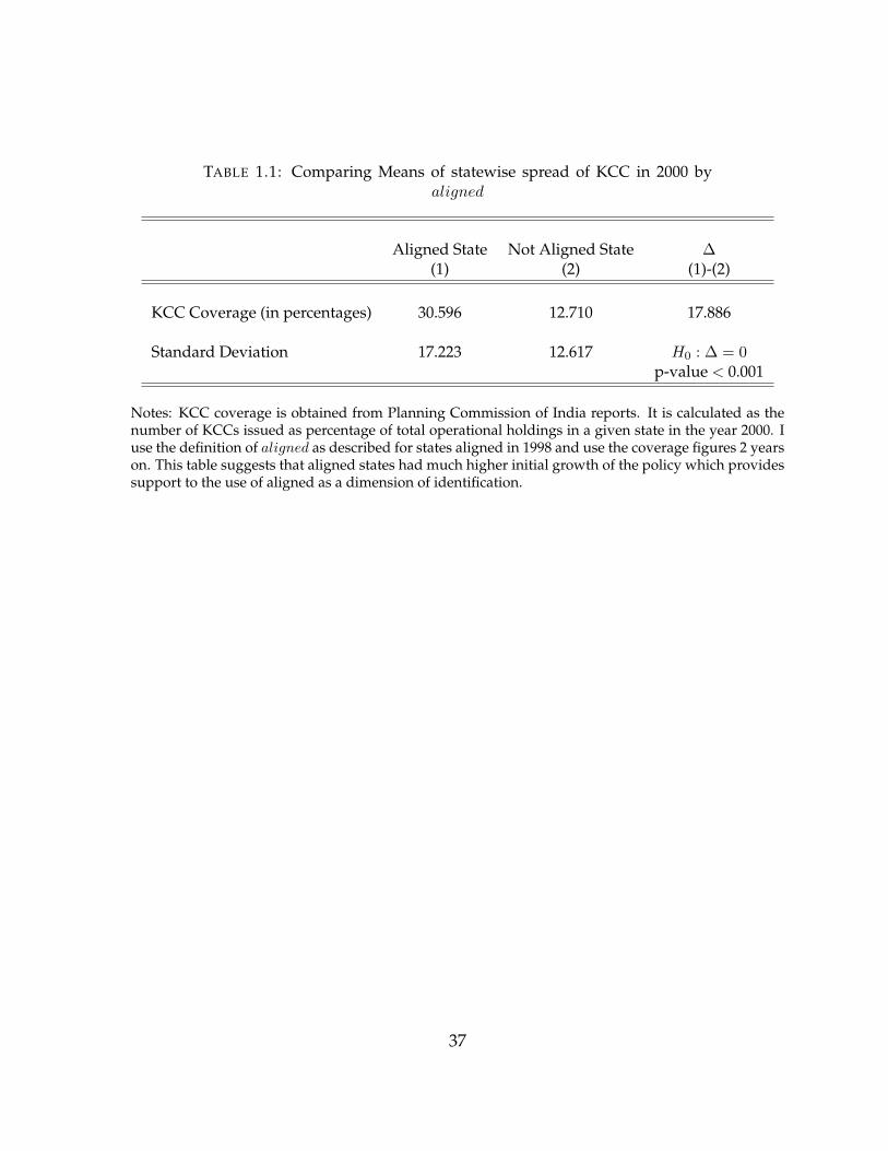
TABLE 1.1: Comparing Means of statewise spread of KCC in 2000 byaligned
Aligned State Not Aligned State ∆(1) (2) (1)-(2)
KCC Coverage (in percentages) 30.596 12.710 17.886
Standard Deviation 17.223 12.617 H0 : ∆ = 0p-value < 0.001
Notes: KCC coverage is obtained from Planning Commission of India reports. It is calculated as thenumber of KCCs issued as percentage of total operational holdings in a given state in the year 2000. Iuse the definition of aligned as described for states aligned in 1998 and use the coverage figures 2 yearson. This table suggests that aligned states had much higher initial growth of the policy which providessupport to the use of aligned as a dimension of identification.
37

FIGURE 1.1: Crop Production: Year-specific coefficients for aligneds ·morebanksd
-100
-50
0
50
100
150
200
250
1986 1991 1996 2001 2006
Maize Production
95% ConfidenceIntervals
-100
-50
0
50
100
150
200
250
1986 1991 1996 2001 2006
Wheat Production
95% ConfidenceIntervals
Notes: The vertical line marks the policy year whereas the dotted line represent 95% confidence intervals. Regressions use the VDSA district panel dataset and control forcrop specific area under production, rainfall, crop specific iirigated area, markets nearby, gross cropped and irrigated areas and state fixed effects.
38

FIGURE 1.2: HYV Use: Year-specific coefficients for aligneds ·morebanksd
Notes: The vertical line marks the policy year whereas the dotted line represent 95% confidence intervals. Regressions use the VDSA district panel dataset and control forrainfall, markets nearby, gross cropped and irrigated areas and state fixed effects.
39
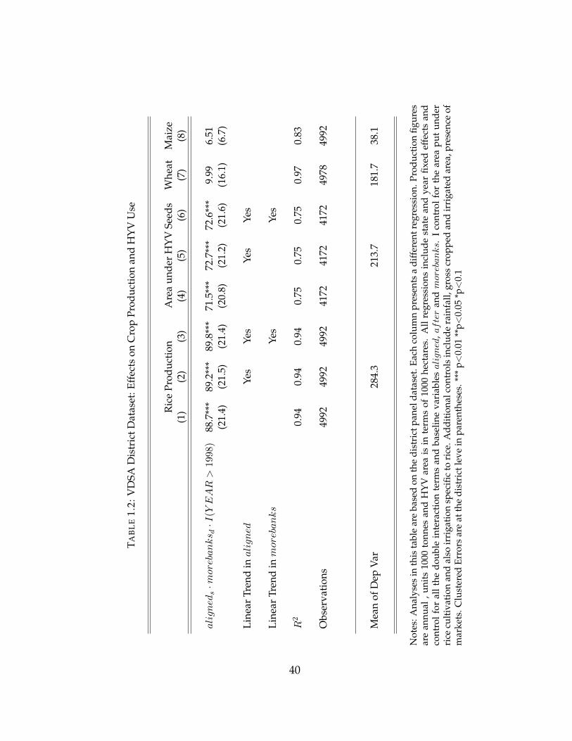
TAB
LE
1.2:
VD
SAD
istr
ictD
atas
et:E
ffec
tson
Cro
pPr
oduc
tion
and
HY
VU
se
Ric
ePr
oduc
tion
Are
aun
der
HY
VSe
eds
Whe
atM
aize
(1)
(2)
(3)
(4)
(5)
(6)
(7)
(8)
aligneds·m
orebanks d·I
(YEAR>
1998
)88
.7**
*89
.2**
*89
.8**
*71
.5**
*72
.7**
*72
.6**
*9.
996.
51(2
1.4)
(21.
5)(2
1.4)
(20.
8)(2
1.2)
(21.
6)(1
6.1)
(6.7
)
Line
arTr
end
inaligned
Yes
Yes
Yes
Yes
Line
arTr
end
inmorebanks
Yes
Yes
R2
0.94
0.94
0.94
0.75
0.75
0.75
0.97
0.83
Obs
erva
tion
s49
9249
9249
9241
7241
7241
7249
7849
92
Mea
nof
Dep
Var
284.
321
3.7
181.
738
.1
Not
es:A
naly
ses
inth
ista
ble
are
base
don
the
dist
rict
pane
ldat
aset
.Eac
hco
lum
npr
esen
tsa
diff
eren
treg
ress
ion.
Prod
ucti
onfig
ures
are
annu
al,u
nits
1000
tonn
esan
dH
YV
area
isin
term
sof
1000
hect
ares
.A
llre
gres
sion
sin
clud
est
ate
and
year
fixed
effe
cts
and
cont
rolf
oral
lthe
doub
lein
tera
ctio
nte
rms
and
base
line
vari
able
saligned
,after
andmorebanks.
Ico
ntro
lfor
the
area
put
unde
rri
cecu
ltiv
atio
nan
dal
soir
riga
tion
spec
ific
tori
ce.A
ddit
iona
lcon
trol
sin
clud
era
infa
ll,gr
oss
crop
ped
and
irri
gate
dar
ea,p
rese
nce
ofm
arke
ts.C
lust
ered
Erro
rsar
eat
the
dist
rict
leve
inpa
rent
hese
s.**
*p<
0.01
**p<
0.05
*p<
0.1
40

TAB
LE
1.3:
IHD
SD
atas
et:E
ffec
tson
Borr
owin
gC
ompo
siti
on
PAN
ELA
IfBo
rrow
sTo
talO
utst
andi
ngD
ebt
Num
ber
ofLo
ans
Mai
nC
redi
tor
isBa
nk
All
Cul
tiva
tor
Ric
eA
llC
ulti
vato
rR
ice
All
Cul
tiva
tor
Ric
eA
llC
ulti
vato
rR
ice
(1)
(2)
(3)
(4)
(5)
6)(7
)(8
)(9
)(1
0)(1
1)(1
2)
aligned·m
orebanks
-0.0
72-0
.059
-0.1
38*
-0.5
14-7
.984
-0.0
27-1
.351
**-0
.998
-1.5
90**
-.039
-.067
-.068
(0.0
49)
(0.0
60)
(0.0
75)
(6.5
89)
(9.4
41)
(9.6
70)
(0.6
51)
(0.6
67)
(0.7
43)
(0.0
23)
(0.0
47)
(0.0
62)
Mea
n0.
458
0.50
80.
509
38.6
3849
.252
34.8
273.
170
3.23
23.
385
0.12
10.
174
0.15
1
Obs
erva
tion
s21
450
7907
5700
1025
040
2126
7810
111
4147
2827
2145
079
0757
00
PAN
ELB
Onl
yLa
rges
tLoa
nsO
nly
Larg
estL
oans
from
Bank
s
Inte
rest
Rat
esLo
anSi
zeIn
tere
stR
ates
Loan
Size
All
Cul
tiva
tor
Ric
eA
llC
ulti
vato
rR
ice
All
Cul
tiva
tor
Ric
eA
llC
ulti
vato
rR
ice
(1)
(2)
(3)
(4)
(5)
6)(7
)(8
)(9
)(1
0)(1
1)(1
2)
aligned·m
orebanks
0.08
00.
014
0.19
29.
414*
**12
.068
16.7
25*
-0.0
37-0
.085
-0.1
1441
.364
***
37.8
17**
44.1
81**
(0.2
39)
(0.2
07)
(0.3
10)
(4.7
59)
(7.6
72)
(10.
197)
(0.0
72)
(0.0
82)
(0.0
82)
(2.9
73)
(14.
576)
(19.
470)
Mea
n2.
105
1.88
62.
157
32.7
1940
.828
32.9
281.
059
1.07
91.
045
62.9
6165
.314
58.9
79
Obs
erva
tion
s10
114
4145
2827
1011
741
5128
7826
9614
3788
026
9614
3788
0
Not
es:E
ach
colu
mn
repr
esen
tsa
diff
eren
treg
ress
ion.
The
sam
ple
inPa
nelB
incl
udes
answ
ers
toqu
esti
ons
abou
tthe
larg
estl
oan
inla
st5
year
sfo
rth
eho
useh
olds
.M
onet
ary
Val
ues
(for
loan
size
and
outs
tand
ing
loan
s)ar
ein
INR
1000
unit
s.C
olum
ns1-
3in
Pane
lAre
port
regr
essi
ons
whe
reth
ede
pend
entv
aria
ble
isa
dum
my
for
whe
ther
the
hous
ehol
dha
san
ybo
rrow
ing
inth
epa
st5
year
s.To
talo
utst
andi
ngde
btis
the
vari
able
for
how
muc
hth
eho
useh
old
curr
entl
yow
esot
hers
cond
itio
nal
onno
n-ze
roou
tsta
ndin
gde
bt.T
henu
mbe
rof
loan
sva
riab
leis
also
wit
hre
spec
tto
num
ber
oflo
ans
inpa
st5
year
s.Th
ede
pend
entv
aria
ble,
Mai
nC
redi
tor
isBa
nk,
isa
dum
my
indi
cati
ngif
the
larg
estl
oan
ofa
borr
ower
com
esfr
oma
bank
and
take
sth
eva
lue
zero
for
borr
ower
sfr
omot
her
sour
ces
asw
ella
sno
nbo
rrow
ers.
The
coef
ficie
nts
repo
rted
are
foraligned·m
orebanks.
All
regr
essi
ons
incl
ude
stat
efix
edef
fect
san
dco
ntro
lfor
base
linemorebanks
vari
able
.A
ddit
iona
ldem
ogra
phic
cont
rols
incl
ude
num
ber
ofpe
rson
sin
each
fam
ily,n
umbe
rof
child
ren
inea
chho
useh
old,
num
ber
ofm
arri
edm
enan
dm
arri
edw
omen
,age
and
educ
atio
nle
vels
ofm
enan
dw
omen
.C
ulti
vato
rre
pres
ents
the
sam
ple
ofho
useh
olds
who
sem
ain
inco
me
sour
ceis
repo
rted
tobe
cult
ivat
ion
and
allie
dag
ricu
ltur
e.R
ice
farm
ers
are
hous
ehol
dsw
hopr
oduc
ea
posi
tive
amou
ntof
rice
.Clu
ster
edSt
anda
rdEr
rors
are
atth
edi
stri
ctle
vel.
***
p<0.
01**
p<0.
05*p<
0.1
41

TAB
LE
1.4:
IHD
SD
atas
et:E
ffec
tson
Ric
ePr
oduc
tion
and
Sale
s
All
Prod
ucer
sIf
Sells
Out
put
Qua
ntit
yQ
uant
ity
Pric
eX
Qua
ntit
y
Full
Sam
ple
Bank
Borr
ower
sFu
llSa
mpl
eBa
nkBo
rrow
ers
Full
Sam
ple
Bank
Borr
ower
s(1
)(2
)(3
)(4
)(5
)(6
)
aligned·m
orebanks
0.91
710
.809
**7.
719
18.9
82**
40.8
810
7.63
**(4
.033
)(5
.299
)(6
.355
)(7
.636
)(3
8.62
)(4
3.12
)
Obs
erva
tion
s71
1899
725
8346
425
8346
4
Mea
n21
.067
25.2
4440
.736
40.3
6523
8.54
228.
67
Not
es:
The
sam
ple
isre
stri
cted
toon
lyri
cefa
rmer
sin
the
IHD
Sda
tase
t.Ea
chco
lum
nre
pres
ents
adi
ffer
entr
egre
ssio
n.A
llre
gres
-si
ons
incl
ude
stat
efix
edef
fect
san
dco
ntro
lfor
base
linemorebanks
vari
able
.A
ddit
iona
ldem
ogra
phic
cont
rols
incl
ude
num
ber
ofpe
rson
sin
each
fam
ily,
num
ber
ofch
ildre
nin
each
hous
ehol
d,nu
mbe
rof
mar
ried
men
and
mar
ried
wom
en,a
gean
ded
ucat
ion
leve
lsof
men
and
wom
enan
dar
eaun
der
rice
prod
ucti
on.T
hede
pend
entv
aria
ble
inco
lum
ns(1
)to
(4)i
sri
cepr
oduc
tion
inte
nths
ofa
quin
tal.
The
depe
nden
tvar
iabl
ein
colu
mn
5is
the
reve
nue
from
sale
ofri
ceco
ndit
iona
lon
selli
ngri
ce.T
heun
its
are
INR
1000
.Ba
nkBo
rrow
ers
repr
esen
tth
esa
mpl
eof
hous
ehol
dsw
hoha
vebo
rrow
edin
the
past
5ye
ars
and
thei
rla
rges
tlo
anco
mes
from
aba
nk.C
lust
ered
stan
dard
erro
rsat
the
dist
rict
leve
lin
pare
nthe
ses.
Num
ber
ofcl
uste
rsis
282.
***
p<0.
01**
p<0.
05*p<
0.1
42

TAB
LE
1.5:
IHD
SD
atas
et:E
ffec
tson
Inco
me
Per
Cap
ita
Inco
me
Per
Cap
ita
Farm
Inco
me
Per
Cap
ita
Non
Farm
Inco
me
All
Cul
tiva
tor
Bank
Borr
ower
All
Cul
tiva
tor
Bank
Borr
ower
sA
llBu
sine
ssPe
rson
(1)
(2)
(3)
(4)
(5)
6)(7
)(8
)
aligned·m
orebanks
-0.0
160.
053
0.32
3*0.
043
0.12
90.
424*
0.03
0.01
2(0
.069
)(0
.141
)(0
.197
)(0
.063
)(0
.140
)(0
.223
)(0
.060
)(0
.159
)
Mea
n0.
715
0.73
10.
951
0.20
70.
476
0.41
10.
463
0.80
8
Obs
erva
tion
s21
117
7634
2634
2029
172
6225
0137
6967
7
Not
es:E
ach
colu
mn
repr
esen
tsa
diff
eren
treg
ress
ion.
The
coef
ficie
nts
repo
rted
are
foraligned·m
orebanks.
All
regr
essi
ons
incl
ude
stat
efix
edef
fect
san
dco
ntro
lfor
base
linemorebanks
vari
able
.Add
itio
nald
emog
raph
icco
ntro
lsin
clud
enu
mbe
rof
pers
ons
inea
chfa
mily
,num
ber
ofch
ildre
nin
each
hous
ehol
d,nu
mbe
rof
mar
ried
men
and
mar
ried
wom
en,a
gean
ded
ucat
ion
leve
lsof
men
and
wom
en.
Inth
ista
ble,
mon
etar
yfig
ures
are
inm
onth
lyIN
R10
00w
hich
isap
prox
mon
thly
USD
20.
The
sam
ple
size
isva
riab
lein
this
tabl
eba
sed
onth
egr
adat
ions
‘ifcu
ltiv
ator
’and
‘ifbu
sine
sspe
rson
’.A
hous
ehol
dis
deno
ted
asa
cult
ivat
orif
the
resp
onde
ntre
port
edth
atth
eir
mai
nin
com
eso
urce
isfr
omcu
ltiv
atio
nor
allie
dac
tivi
ties
.Si
mila
rly
ifth
ere
port
edm
ain
sour
ceof
inco
me
isbu
sine
ss,I
clas
sify
thes
eho
useh
olds
as‘b
usin
ess
pers
ons’
.Ban
kBo
rrow
ers
repr
esen
tthe
sam
ple
ofho
useh
olds
who
have
borr
owed
inth
epa
st5
year
san
dth
eir
larg
estl
oan
com
esfr
oma
bank
.Clu
ster
edSt
anda
rdEr
rors
are
atth
edi
stri
ctle
vel.
***
p<0.
01**
p<0.
05*p<
0.1
43

TAB
LE
1.6:
IHD
SD
atas
et:E
ffec
tson
Con
sum
ptio
nEx
pend
itur
e
Per
Cap
ita
Mon
thly
Con
sH
ouse
hold
Item
sTe
mpt
atio
nG
oods
All
Cul
tiva
tor
Bank
Borr
ower
sA
llC
ulti
vato
rBa
nkBo
rrow
ers
All
Cul
tiva
tor
Bank
Borr
ower
s(1
)(2
)(3
)(4
)(5
)6)
(7)
(8)
(9)
aligned·m
orebanks
-0.0
019
0.00
020.
0084
0.01
130.
0161
*0.
0215
**-0
.028
3***
-0.0
360*
**-0
.011
4(0
.003
7)(0
.006
4)(0
.007
4)(0
.007
3)(0
.009
3)(0
.010
8)(0
.010
3)(0
.012
5)(0
.017
8)
Mea
n0.
0644
0.06
580.
0854
0.07
290.
0791
0.08
770.
0817
0.08
290.
0928
Obs
erva
tion
s21
437
7899
2695
2143
778
9926
9521
437
7899
2695
Not
es:E
ach
colu
mn
repr
esen
tsa
diff
eren
treg
ress
ion.
The
coef
ficie
nts
repo
rted
are
foraligned·m
orebanks.
All
regr
essi
ons
incl
ude
stat
efix
edef
fect
san
dco
ntro
lfor
base
linemorebanks
vari
able
.Add
itio
nald
emog
raph
icco
ntro
lsin
clud
enu
mbe
rof
pers
ons
inea
chfa
mily
,num
ber
ofch
ildre
nin
each
hous
ehol
d,nu
mbe
rof
mar
ried
men
and
mar
ried
wom
en,a
gean
ded
ucat
ion
leve
lsof
men
and
wom
en.M
onet
ary
figur
esar
ein
INR
1000
unit
she
re.T
hete
mpt
atio
ngo
ods
incl
ude
beet
elle
aves
/tob
acco
etc.
Bane
rjee
etal
(201
5)fin
dth
atm
icro
finan
ceas
adi
scip
linin
gde
vice
redu
ces
per
capi
taco
nsum
ptio
nof
thes
ego
ods
byIN
R9.
The
per
capi
tale
quiv
alen
tof
my
findi
ngof
INR
28re
duct
ion
isIN
R4.
The
HH
item
sin
clud
ere
gula
rpu
rcha
ses
like
soap
s,bu
lbs,
buck
ets,
inse
ctic
ides
etc.
Iuse
the
IHD
S20
05sa
mpl
eof
rura
lhou
seho
lds
whi
chha
ve26
734
obse
rvat
ions
.C
ulti
vato
rre
pres
ents
the
sam
ple
ofho
useh
olds
who
sem
ain
inco
me
sour
ceis
repo
rted
tobe
cult
ivat
ion
and
allie
dag
ricu
ltur
e.Ba
nkBo
rrow
ers
repr
esen
tth
esa
mpl
eof
hous
ehol
dsw
hoha
vebo
rrow
edin
the
past
5ye
ars
and
thei
rla
rges
tloa
nco
mes
from
aba
nk.
Clu
ster
edSt
anda
rdEr
rors
are
atth
edi
stri
ctle
vel.
***
p<0.
01**
p<0.
05*p<
0.1
44

TAB
LE
1.7:
Fals
ifica
tion
Exer
cise
1993
2005
2005
Com
para
ble
Con
trol
sA
llC
ontr
ols
(1)
(2)
(3)
Per
Cap
ita
Mon
thly
Inco
me
0.01
90.
094
0.12
7(0
.045
)(0
.125
)(0
.120
)
Per
Cap
ita
Mon
thly
Inco
me
(ifp
rinc
ipal
occu
pati
onis
cult
ivat
ion)
0.03
70.
292
0.32
9(0
.064
)(0
.198
)(0
.191
)
Not
es:I
run
redu
ced
form
regr
essi
ons
follo
win
gth
esa
me
iden
tific
atio
nst
rate
gyas
desc
ribe
din
the
text
for
2005
and
usin
gth
eH
DPI
data
from
1993
.Ius
eth
esa
me
hous
ehol
ds(8
947)
for
both
year
s.Fo
rth
esa
mpl
elo
okin
gon
lyat
cult
ivat
ors,
Ihav
e37
31ho
useh
olds
.In
colu
mns
1an
d2,
Irun
regr
essi
ons
usin
gon
lyth
eco
mpa
rabl
eco
ntro
lsw
hich
are
age,
educ
atio
nof
mal
e,ed
ucat
ion
offe
mal
ean
dst
ate
fixed
effe
cts.
Inco
lum
n3,
Ire-
run
regr
essi
ons
ofco
lum
n2
usin
gth
esa
me
sam
ple
buta
ddin
gth
eco
ntro
lsus
edin
the
orig
inal
anal
ysis
whi
char
eav
aial
able
for
2005
.The
addi
tion
alco
ntro
lsin
colu
mn
3ar
enu
mbe
rof
pers
ons
infa
mily
,num
ber
ofch
ildre
nan
dnu
mbe
rof
mar
ried
mal
esan
dfe
mal
es.
Ion
lyre
port
the
com
para
ble
outc
ome
vari
able
s.C
lust
ered
stan
dard
erro
rsat
the
dist
rict
leve
lin
pare
nthe
ses.
***
p<0.
01**
p<0.
05*p<
0.1
45

46
Chapter 2
“None of the Above" Votes in India and
the Consumption Utility of Voting(with Gergely Ujhelyi and Andrea Szabó)
2.1 Introduction
One possible solution to the “paradox” of why people bother to vote in large elections
is that voting yields consumption utility. Such consumption utility could be derived
from performing one’s civic duty, expressing one’s political views, or participating
in a democracy (Downs, 1957; Riker and Ordeshook, 1968; Brennan and Lomasky,
1993). Empirically distinguishing these consumption motives from each-other and
from other possible goals, such as a desire to affect the electoral outcome, is notori-
ously difficult. In this paper we propose to do this by using data from a natural ex-
periment in Indian elections and estimating a structural model of voter turnout using
techniques from the consumer demand literature.
We propose to identify different components of the consumption utility of voting
by exploiting a natural experiment in the world’s largest democracy. Following a

decision by the Indian Supreme Court, since September 2013 all state and national
elections in the country must offer a “None Of The Above” (NOTA) option to voters.
Votes cast for NOTA are counted (rather than simply discarded as invalid) but do not
affect the outcome of the election (the winner is still the candidate with a plurality of
votes among votes cast for candidates). In the five states that held local elections after
the Supreme Court ruling 1.7 million voters chose NOTA, and in the 2014 national
election 6 million voters voted for this option (representing 1.1% of all votes cast).
While elections with a NOTA-type option have been used elsewhere, none of them
came close to the scale of the Indian experiment.1
Because in the Indian system NOTA votes cannot affect the outcome of the elec-
tion, voters who choose this option must be motivated by a consumption utility to
vote. Such consumption utility can arise from two broad sources. It can be a general
utility obtained from showing up at the polls (such as complying with a social norm
to participate in the election), or it can be a utility specific to the option chosen by the
voter (such as utility derived from expressing one’s views).
Intuitively, we can distinguish between these two types of consumption utility by
asking how a NOTA-voter would have behaved in the absence of the NOTA option.
If without the NOTA option this voter would have voted for one of the candidates,
this is consistent with both a general and an option-specific utility of voting. By con-
trast if without NOTA this voter would have abstained, then the NOTA vote cannot
be explained by a general utility derived from showing up at the polls. Instead, the
voter must be voting for NOTA in order to obtain a utility specific to this option. Thus,
1In most elections the only way for a voter to participate without voting for a candidate is to cast aninvalid vote and these are difficult to distinguish from voting mistakes. In systems where a NOTA-typeoption is explicitly available to voters, it typically has electoral consequences, affecting who gets electedor whether the election has to be repeated. We review these different systems in section 2.3 below.
47
studying the counterfactual behavior of NOTA voters can test apart these two compo-
nents of the consumption utility from voting.
Our empirical work seeks to test whether, following the introduction of NOTA,
new voters showed up at the polls in order to vote for this option. This question
is challenging because it requires making statements about individual voter behavior
in the counterfactual no-NOTA scenario. Because ballots are secret, individual voter
behavior is observed neither with nor without the NOTA option. Instead, it must be
inferred from aggregate data.
To begin, we first ignore individual behavior and study the impact of NOTA on
aggregate turnout in a reduced form framework. This exercise exploits variation in
the effective timing of the NOTA reform created by the Indian electoral calendar: elec-
tions to the states’ legislative assemblies occur at different times in different states.
This allows us to study the impact of NOTA in a difference-in-differences framework
by comparing the change in voter turnout in states not yet affected by the policy to
changes in those that were already affected. From this analysis we estimate that, in the
average electoral district, the introduction of the NOTA policy significantly increased
turnout. This finding survives a variety of robustness checks and the magnitude of
the effect (2-3 percentage points) is similar to the vote share of NOTA observed in the
data.
While suggestive of new voters turning out to vote for NOTA, these aggregate pat-
terns do not provide conclusive evidence because they mask the substitution between
abstention, candidates, and NOTA at the individual level. To study this, we relate
the aggregate voting returns to individual voter behavior using a structural model
of voter demand for candidates. We adapt the BLP model of Berry, Levinsohn and
48

Pakes (1995) from the consumer demand literature, where consumers (voters) choose
between the products (candidates) of firms (parties) in various markets (electoral dis-
tricts). Voters have preferences over observed and unobserved candidate characteris-
tics (including NOTA) and abstention. The model explicitly allows for heterogeneity
in these preferences and links them to the aggregate vote shares we observe in the
data. Estimating the model allows us to recover the parameters of individual voters’
utility functions from this aggregate data. Using the estimates, we study how voters
substitute between choosing NOTA, one of the candidates, and abstention in counter-
factual simulations where the NOTA option is removed.
The results of this analysis indicate that NOTA increased turnout, which is in line
with the aggregate patterns observed in the reduced form exercise. Furthermore we
find that the magnitude of this increase explains virtually all the NOTA votes ob-
served in the data. We find negligible substitution towards NOTA away from the
candidates running for election. These results indicate that most voters who voted for
NOTA would normally abstain. In turn, this provides evidence for the existence of
consumption utility specifically from voting for NOTA. In this context, models that
do not include an option-specific utility of voting would have a hard time explaining
the data.
To the extent that participation in a democracy is valuable, our finding that having
a NOTA option on the ballot can increase voter turnout is relevant in its own right,
and provides support for the arguments of the Indian Supreme Court in introducing
this policy.
Our paper is related to the vast literature on voter turnout, some of which we
review in section 2.2 below. Instead of proposing a new model of turnout, we focus on
49

testing models apart by asking whether the presence of consumption utility specific to
the NOTA option (as opposed to consumption utility from simply showing up at the
polls) is necessary to explain our data. This approach is similar in spirit to Coate and
Conlin (2004) and Coate et al. (2008) who estimate and compare competing structural
models of turnout on data from Texas liquor referenda.
Methodologically, our paper offers a novel way to estimate vote returns in multi-
party elections. Some earlier approaches to this problem (e.g., Glasgow and Alvarez,
2005) have used discrete choice models with individual-level survey data, but such
data is subject to well-known biases in voters’ self-reported behavior (see, e.g., Selb
and Munzert (2013) and the literature cited therein). Other studies use aggregate ad-
ministrative data and purely statistical models to deal with the problem of conducting
“ecological inference” regarding voter preferences (see Cho and Manski (2008) for a
review). By contrast our BLP-based approach combines the advantages of a micro-
founded discrete choice model with those of aggregate administrative data. It allows
for rich heterogeneity in voter tastes for candidate characteristics and, because it is
micro-founded, offers the possibility of conducting counterfactual experiments. In
a different context, Rekkas (2007) also exploits some of these advantages of the BLP
model in her study of campaign expenditures in the 1997 Canadian election. Our pa-
per goes further by using panel data, allowing for heterogeneity in voters’ preferences
driven by demographics as in Nevo (2001), allowing for endogenous candidate choice
by the competing parties, and by conducting counterfactual experiments using the
estimated model.
Finally, our paper relates to previous studies of NOTA-type votes in the political
science literature (reviewed in section 2.3 below). We differ from this literature by
50
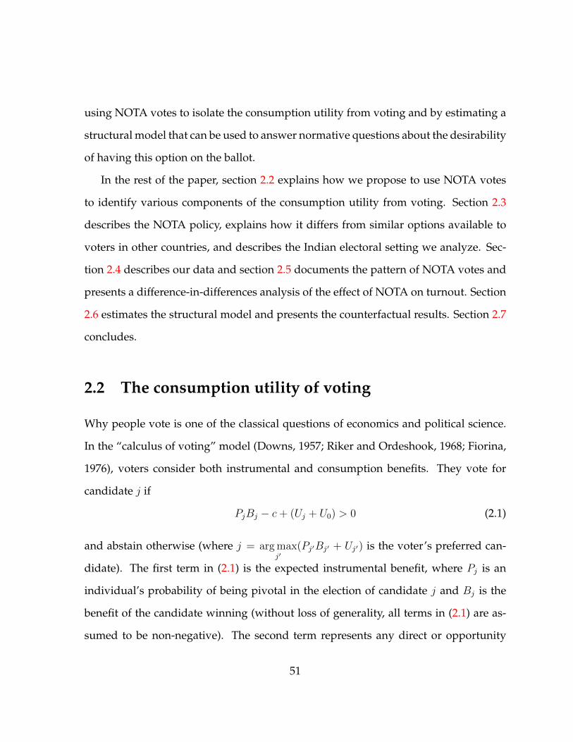
using NOTA votes to isolate the consumption utility from voting and by estimating a
structural model that can be used to answer normative questions about the desirability
of having this option on the ballot.
In the rest of the paper, section 2.2 explains how we propose to use NOTA votes
to identify various components of the consumption utility from voting. Section 2.3
describes the NOTA policy, explains how it differs from similar options available to
voters in other countries, and describes the Indian electoral setting we analyze. Sec-
tion 2.4 describes our data and section 2.5 documents the pattern of NOTA votes and
presents a difference-in-differences analysis of the effect of NOTA on turnout. Section
2.6 estimates the structural model and presents the counterfactual results. Section 2.7
concludes.
2.2 The consumption utility of voting
Why people vote is one of the classical questions of economics and political science.
In the “calculus of voting” model (Downs, 1957; Riker and Ordeshook, 1968; Fiorina,
1976), voters consider both instrumental and consumption benefits. They vote for
candidate j if
PjBj − c+ (Uj + U0) > 0 (2.1)
and abstain otherwise (where j = arg maxj′
(Pj′Bj′ + Uj′) is the voter’s preferred can-
didate). The first term in (2.1) is the expected instrumental benefit, where Pj is an
individual’s probability of being pivotal in the election of candidate j and Bj is the
benefit of the candidate winning (without loss of generality, all terms in (2.1) are as-
sumed to be non-negative). The second term represents any direct or opportunity
51

costs from voting. The final term is the consumption utility of voting, which captures
a wide range of factors sometimes referred to as “expressive utility” or “civic duty”:
“1. the satisfaction from compliance with the ethic of voting [...] 2. the satisfaction
from affirming allegiance to the political system [...] 3. the satisfaction from affirm-
ing a partisan preference [...] 4. the satisfaction of deciding, going to the polls, etc.
[...] 5. the satisfaction of affirming one’s efficacy in the political system” (Riker and
Ordeshook, 1968, p28). We separate this consumption utility into two components to
highlight that part of the utility (Uj) may depend on voting for a specific candidate
j (e.g., the satisfaction from expressing partisan support), while part of it (U0) only
depends on showing up at the polls regardless of who one votes for (e.g., satisfaction
from compliance with an ethical norm to vote).
Observing that in large elections the probability Pj of being pivotal is close to 0,
the recent literature seeking to explain turnout within the framework of the calculus
of voting equation (2.1) has followed various routes.2 First, voters could overestimate
Pj . Lab experiments show that, indeed, voters often overestimate the probability that
their vote will matter and suggest that this can explain turnout decisions (Duffy and
Tavits, 2008; Dittman et al., 2014). Relatedly, Ortoleva and Snowberg (2015) show
that turnout is higher in populations with more overconfident voters. Under these
conditions, turnout can be explained even if (Uj + U0) = 0.
A second set of studies present models that create an option-specific utility Uj . In
2Missing from equation (2.1) are instrumental motivations other than those related to winning. Forexample, it is possible that a voter votes in order to signal his preferences to affect the policies chosenafter the election. Or he may vote in order to encourage a candidate to run again in the future. Itis possible to treat such motivations in a strategic setting but the likelihood that a voter’s vote willbe pivotal in affecting policy or encouraging a candidate is likely to be small (see, e.g., Razin (2003)).Here we follow most of the literature in assuming that if such motivations exist, they are sources ofconsumption utility and hence part of Uj .
52

Coate and Conlin (2004) and Feddersen and Sandorini (2006), this utility represents
ethical considerations regarding what would be best for everyone in one’s group. In
other models, such as Shachar and Nalebuff (1999), Uj is created by the mobilization
efforts of political leaders. In Degan and Merlo (2011), Uj includes a psychological
disutility from the possibility of voting for the “wrong” candidate.
Another set of papers focus on the general utility U0 from showing up to vote.
For example, members of a group may observe turnout and draw inferences about
whether an individual is an “ethical type” (Bénabou and Tirole, 2006; Ali and Lin,
2013). Similarly, a voter may vote to avoid a feeling of shame from not having done
his duty, especially if others will ask whether one has voted (Harbaugh, 1996; Blais,
2000; DellaVigna et al., 2015).
While these studies convincingly demonstrate that the proposed models have ex-
planatory power, it is not always clear to what extent these models are necessary to
explain the data.3 In particular, can we rule out that one or both components of the
consumption utility Uj + U0 is 0?
As we explain below, the Indian NOTA policy allows us to study this question by
creating a “None Of The Above” option that voters can vote for but that, by design,
cannot affect the electoral outcome. First, we document that voters actually choose
NOTA. Because PNOTABNOTA = 0, from equation (2.1) a voter who chooses NOTA
must have
UNOTA + U0 > c (2.2)
i.e., there has to be a positive consumption utility of voting.
3Examples of papers that highlight the value of testing models apart include the pair of studies byCoate and Conlin (2004) and Coate, Conlin, and Moro (2008) which explicitly compare several differentmodels of turnout on the same dataset.
53

Second, we ask how a voter who chose NOTA would have voted in the absence of
the NOTA option. If the voter would have abstained, then PjBj − c + (Uj + U0) ≤ 0.
Combining with (2.2), we have
UNOTA > PjBj + Uj,
i.e., there has to be a positive option-specifc utility from voting for NOTA. For exam-
ple, a voter may derive utility from expressing his disapproval of all the candidates.
Conversely, if in the absence of NOTA the voter would have voted for one of the candi-
dates, then it is possible that there is no option-specific utility but U0 > 0 (for example,
a voter may vote to satisfy social pressure while deriving no specific utility from vot-
ing for any of the options on the ballot.). Thus, studying voters’ behavior with and
without NOTA offers a test for the existence of an option-specific utility of voting.
In this way, although not an actual candidate, studying NOTA votes gives us an
opportunity to test both for the existence of a consumption utility from voting and for
the existence of a consumption utility from voting for this particular option.4 The sec-
ond exercise is empirically challenging because it requires making statements about
individual behavior both with and without NOTA while, due to the secret ballot, such
behavior is never observed.4It is difficult to imagine a similar experiment where an actual candidate’s probability of wining
is administratively set to 0. (Having small-party candidates on the ballot who have little chance ofwinning is not the same experiment since voters’ believing that Pj > 0 cannot be ruled out.) Anotherpossibility is to run a lab experiment where Pj is set to 0, but creating an artificial environment wherepeople derive utility from voting may be difficult. In an interesting experiment Shayo and Harel (2012)create variation in P and find evidence that the moral superiority of an alternative affects voters’ be-havior when P is small.
54

2.3 Background
2.3.1 The Indian NOTA policy
In elections where a paper ballot is used, voters can participate without voting for
any of the candidates: they can hand in an empty ballot or otherwise intentionally
invalidate their vote. With the advent of electronic voting machines Indian voters
lost this possibility. In 2004, the citizen’s group People’s Union for Civil Liberties
(PUCL) filed a petition with the Supreme Court to rectify this and give voters the
ability to have their participation recorded without forcing them to vote on any of the
candidates.5 In its 2013 decision, the Supreme Court agreed:
“For democracy to survive, it is essential that the best available men
should be chosen as people’s representatives for proper governance of the
country. This can be best achieved through men of high moral and ethical
values, who win the elections on a positive vote. Thus in a vibrant democ-
racy, the voter must be given an opportunity to choose none of the above
[...] Democracy is all about choice. This choice can be better expressed by
giving the voters an opportunity to verbalize themselves unreservedly and
by imposing least restrictions on their ability to make such a choice. By pro-
viding NOTA button in the Electronic Voting Machines, it will accelerate
5Under the electronic voting machines, the only way for a voter to have his non-vote recorded wasto inform the clerk at the voting booth of his desire to do so. The clerk would then record this on thevoter ledger together with the voter’s thumbprint for identification. The PUCL argued that this wasunconstitutional, violating the secret ballot.
55

the effective political participation in the present state of democratic sys-
tem and the voters in fact will be empowered.” (PUCL vs. Union of India,
2013, p43-44).
Following the Supreme Court’s decision, since September 2013, all state and na-
tional elections in India give voters the option of recording a “None Of The Above”
vote on the voting machine. These votes are counted and reported separately but have
no role in the outcome of the election. In particular, votes cast on NOTA affect neither
the validity nor the winner of an election. Even if NOTA were to receive a majority
of the votes, the winner of the election would be the candidate who received the most
votes among the non-NOTA votes.
The NOTA policy received wide news coverage in both national and local me-
dia. In its decision the Supreme Court directed the Election Commission to undertake
awareness programs to inform the electorate of the new policy, and voter education
programs explicitly focused on explaining this new option to voters. As a result we
expect that most voters would be well-informed about the NOTA policy, including the
fact that NOTA votes would not affect the electoral outcome.6
2.3.2 NOTA-like options in other countries
In most countries voters can effectively cast a “none of the above” vote by intentionally
returning an invalid vote (e.g., leaving the ballot blank, writing on the ballot, or mark-
ing more than one candidate). Because it is typically impossible to know whether such
votes occur intentionally or by mistake, it is difficult to use them to draw conclusions
regarding voters’ intentional behavior (see, e.g., McAllister and Makkai, 1993; Herron6As we discuss in section 2.5, several patterns in the data also support this assumption.
56

and Sekhon, 2005; Power and Garand, 2007; Uggla, 2008; Driscoll and Nelson, 2014).
For some applications, the fact that invalid votes also include voting mistakes will
simply add measurement error to the “true” measure intended to capture negative
votes. In other cases, however, this will have an important impact on the interpreta-
tion of the results. For example, more invalid votes among the less educated can mean
either that these voters are more likely to make mistakes when filling out the ballot, or
they are particularly dissatisfied and intentionally cast invalid votes to express this.7
In some countries, while there is no NOTA option on the ballot, blank votes are
counted separately from invalid votes and are believed to represent a negative vote.
In principle, this system could be equivalent to the Indian NOTA, but in practice the
equivalence is unlikely to be perfect. First, blank votes could still represent voting
mistakes, especially if there is a judgement call to be made about whether a vote is
truly blank when it is being counted (for example, there could be markings on the
side of the ballot, a small dot inside the checkbox, etc.). Fujiwara (2015) finds that
the introduction of voting machines in Brazil reduced both blank and invalid votes
among the less educated, which is consistent with both of these containing voting
mistakes. Second, using the blank vote as an expression of dissatisfaction requires
a shared understanding among voters regarding what the vote represents. Whether
this social norm is operative in a given election is difficult to test. This is illustrated
by the findings of Superti (2015) who studies a set of municipal elections in Spain - a
country where the blank vote is generally understood to mean “none of the above.”
She shows that despite this common understanding, voter dissatisfaction following
7These two interpretations also have different welfare implications regarding the desirability of hav-ing a NOTA option on the ballot. In the first case, NOTA only serves to confuse the less educated; inthe second case, it gives disadvantaged segments of the population a voice.
57

a ban which prevented the Basque nationalist party from contesting an election was
likely expressed through an increase in invalid rather than blank votes.
Another feature that makes India a cleaner case study than other systems for the
analysis of voters’ motivations is the electoral impact of the NOTA vote. Recall that in
India the NOTA vote can never “win,” and due to the first-past-the-post system it has
no impact on the allocation of legislative seats. By contrast in Colombia if the “blank
vote” wins, new elections must be called with the rejected candidates prohibited from
running again. In Spain, while the blank vote can never win, seats are allocated in
a proportional system and a minimum 3% threshold must be reached for a party to
enter parliament. In both of these systems choosing the blank vote as opposed to
choosing one of the parties has immediate electoral consequences, affecting the mix
of candidates eventually elected for office. In the Indian case, NOTA votes cannot be
driven by electoral motivations in the current election.8
2.3.3 Assembly elections in India
We study voters’ behavior under NOTA in the context of Indian state elections. In
the Indian federal system, state governments are responsible for most areas of local
significance, including health care, education, public works, police and security, and
disaster management. State legislative assemblies are elected in single-member elec-
toral districts (called “constituencies”) in a first-past-the-post system. The party or
8A voter’s motivation (with any vote under any system) can always include a desire to affect long-run outcomes, e.g., by signaling his political preferences to the eventual winner in order to affect policy,or by encouraging a candidate to run in future elections. Because a single vote is just as unlikely to bepivotal in affecting these outcomes as it is in affecting who wins, we think that these motivations arebest viewed as alternative sources of the consumption utility derived from voting.
58

coalition that wins the most number of seats in an assembly forms the state govern-
ment headed by a Chief Minister and his council of ministers.9
Table 2.1 shows the timing of state assembly elections in our study period. Elec-
tions are held every 5 years but the electoral calendar varies widely across states. For
example some states held assembly elections in 2007 and 2012 while others in 2008
and 2013; some states always go to the polls in March while others always do so in
November. This variation in the timing of elections creates an important source of
identification for the analysis below.
In most states assembly elections are conducted separately from other elections.
Four states, Andhra Pradesh, Arunachal Pradesh, Odisha and Sikkim, hold elections
simultaneously with national elections. We will exclude these states from the analysis
below.
All state and national elections in India are conducted by the Election Commission
of India under the supervision of the chief election commissioner. Since independence,
the Commission has emerged as a highly regarded institution with a large degree
of autonomy (McMillan, 2010). Election dates are set well in advance and declared
as local holidays to reduce the cost of participation. Polling stations (“booths”) are
spread out throughout each constituency and enlisted voters are assigned to specific
booths. Voters go to their designated booth to cast their vote with their Elector’s Photo
Identification Card.10 Generally these booths are set up in neighboring schools or
9In states that have a bicameral legislature, the system just described applies to the lower house.Members of the upper house are either elected by the lower house or appointed by the Chief Ministeror the Governor (the representative of the federal government in the states).
10Voter Registration is a one time procedure. Except in special cases (such as for convicted criminals),once registered as a voter, a person can vote in all subsequent elections without having to go throughany further registration process. Once registered the voter’s name is on the voters’ list and he or shegets the identification card which needs to be produced at the polling station before being allowed tovote.
59

public buildings within a very small radius of one’s residence. Participation rates in
Indian elections tend to be high. In our state election data, average turnout is 71% and
only 7% of the constituencies had turnout lower than 50%. (By comparison turnout in
US midterm elections is typically around 40%.) The voting age is 18, and the average
constituency has approximately 180 thousand eligible voters.
Since 2004 all voting in India has taken place using electronic voting machines
(EVMs).11 Each candidate running in an election has a separate button assigned to
him on the machine. Next to the button is the symbol identifying the candidate (to
accommodate illiterate voters) and the voter pushes the button to record his vote. A
light illuminates confirming that the vote was successful.12 Under the NOTA policy,
one of the buttons on the machine is assigned to the NOTA option.
In the system of political reservation, some constituencies are designated Sched-
uled Caste (SC) and some Scheduled Tribe (ST). In these, only candidates from the
given caste can run (to win, they must still obtain a plurality of all votes regardless of
voters’ caste). The reserved status of SC and ST constituencies is set at the same time
as the electoral boundaries are drawn. In contrast to local (village) governments, state
elections have no political reservation for women.
The current electoral constituencies were set in April 2008 by a commission work-
ing under the Election Commission (see Table 2.1). This was the first time in over 30
years that electoral redistricting (“delimitation”) took place in India. All constituency
boundaries as well as the reservation status of the constituencies was fixed by the de-
limitation commission in order to reflect population figures of the 2001 census. As
11Electronic voting machines in India were introduced gradually beginning in 1999. Since 2004 allgeneral and state elections are conducted using these machines.
12These machines are simpler to operate than some of the EVMs used in other countries that some-times require a voter to follow written instructions, enter a candidate’s number on a keypad, etc.
60

described below, this redistricting poses challenges for the construction of our dataset
and our empirical strategy.
2.4 Data
2.4.1 Samples used for analysis
Our analysis uses two samples of constituencies: a panel serves as our primary dataset,
and we use a repeated cross-section as a secondary sample.
The instrumental variables used in the structural analysis require panel data, and
our main sample is a constituency level panel dataset of the 6 states that conducted
assembly elections in both 2008 and 2013 under the new electoral boundaries: Kar-
nataka, Chhattisgarh, Rajasthan, Madhya Pradesh, Delhi, and Mizoram (see Table 2.1).
One of these states, Karnataka held elections in both years without a NOTA option,
while the remaining 5 states had a NOTA option in 2013 but not in 2008.
The main obstacle to extending the panel data to more constituencies is the delim-
itation (electoral redistricting). This makes it impossible to include elections before
April 2008 in the panel as there is too little overlap between the old and new con-
stituencies to make constituency-level matching meaningful.13 For example, although
3 other states also held elections in both 2008 and 2013, they did so in February-March
and had their constituency boundaries redrawn between the two elections in April
13Using GIS software we have computed the maximum overlap of each current constituency’s areawith an old constituency. For example, a maximum overlap of 80% indicates that 80% of the currentconstituency’s area came from one constituency, while 20% came from one or more other constituencies.We find that half of the current constituencies have a maximum overlap of 62% or less and a quarter ofthe constituencies have a maximum overlap of 50% or less. This makes it impossible to match electoraldata across constituencies in a meaningful way.
61

2008 so we cannot include these states in the panel. Other states with consistent elec-
toral boundaries in our study period are those holding elections in 2014. However,
2014 was a national election year that made headlines around the world for its un-
usual outcome (the BJP led by Narendra Modi won by a landslide, the first time in 30
years that a single party won a majority of the legislative seats). Because 2014 state
assembly elections took place either simultaneously with or after the national election
(and in the latter case more than a year after the NOTA policy was introduced), the
national election could confound the impact of NOTA in these states. We therefore
decided to exclude these states from the panel analysis.
To obtain more power for a reduced form analysis, we use as a secondary dataset a
repeated cross section of constituencies in 25 states that conducted elections between
2006 and 2014. Like the panel, this dataset excludes the states that held assembly elec-
tions simultaneously with national elections (Andhra Pradesh, Arunachal Pradesh,
Odisha and Sikkim) since turnout considerations in these states are likely to be very
different.14 It also excludes the state of Bihar because its unique election calendar (2005
and 2010) would require earlier data on voter demographics than we have access to.
We next describe the information available in the primary (panel) and secondary
(repeated cross-section) datasets.
2.4.2 Election data
The electoral data comes from the Election Commission of India, which provides in-
formation on assembly elections at the candidate level. For each constituency we
14Since our main goal with the repeated cross section is to increase power, we include the states thatheld elections in 2014 but not simultaneously with the national election. Excluding these states makeslittle difference for the results.
62

know the list of candidates running, their party, age, gender, and caste (General, ST or
SC). We also know the number of votes received by each candidate (including NOTA
for the relevant elections) as well as the number of eligible voters in each constituency.
Table 2.2 shows summary statistics of the electoral data at the constituency level
for the panel and the repeated cross section. In the 6-state panel, for each year there
are 854 constituencies. In 2013, 630 of these constituencies were affected by NOTA
because state elections were held after the Supreme Court decision. In the repeated
cross section, we have a total of 6685 constituency-year observations from 25 states.
1176 of these observations were affected by NOTA in either 2013 or 2014. The average
constituency has approximately 180 thousand eligible voters and 11 candidates com-
peting. The overwhelming majority of candidates are male: the average constituency
has less than one female candidate. The median age of candidates in a constituency
is typically between 38 and 53. Approximately 13% of the constituencies are reserved
for SC and 15% for ST. The average non-reserved constituency has 1.3 SC candidates
and less than 0.5 ST candidates. Average turnout is 71% and the average vote share of
the winning candidate is 45%. Summary statistics of the electoral data in the 6-state
panel and the 25-state repeated cross section tend to be similar.
Table 2.3 shows a more detailed distribution of candidate characteristics in the
panel dataset. Each year we have approximately 10,000 candidates in this dataset.
40% of these candidates run as independents not affiliated with any party.
2.4.3 Voter demographics
Our first source of demographic information is various waves of the National Sample
Survey, conducted by the Indian Ministry of Statistics and Program Implementation
63

since 1950. Each wave contains close to half a million individual surveys covering all
Indian states, and is designed to be representative of the population at the subdistrict
level. We obtained the individual level data and use it to create characteristics of the
voting age population at the state-year or the district-year level for the reduced-form
analysis. Table 2.4 summarizes these variables for the 25 states in the repeated cross
section. We complement this with data on the growth rate of per capita state domestic
product from the Reserve Bank of India.
For the structural exercise, demographic characteristics are needed at the con-
stituency level. We are not aware of any existing dataset with appropriate coverage.
We create the necessary dataset using the 2011 Indian Census by aggregating village-
level information and matching it to constituencies using GIS coordinates. Specifically,
we obtained GIS boundary files for the 2013 electoral constituencies and the 2001 cen-
sus. To use data from the 2011 census, we proceed in two steps. First, we match
sub-districts (“tehsil”) in the 2001 census to the 2011 census using village names.15
Administrative boundaries in India change over time, with tehsils, districts, and even
states splitting up into new units. This step of our matching procedure is based on
the smallest administrative unit available in the census, the village. Second, we match
the 2011 census data to each 2013 electoral constituency using the 2001 sub-district
boundaries. We use area-weighted averages to compute values for constituencies that
overlap several sub-districts.
Of the 854 constituencies, we have constituency boundary files for 850. We were
able to match 723 of these to the sub-district data from the census. The location of
these constituencies is shown on Figure 2.1. Most of the constituencies we lose during
15Sub-districts, called tehsils in most states, are administrative units above the villages and below thedistricts and the states.
64

the matching (70) are in NCT Delhi. We lose this entire state because the census data
is not sufficiently disaggregated. Of the matched constituencies, 520 are affected by
NOTA in 2013 and 203 are not (in the full panel, these numbers are respectively 630
and 224).
Table 2.5 shows the summary statistics of the census data at the constituency level.
The variables include basic demographic characteristics such as gender, caste, literacy,
and employment as well as economic characteristics of the households (infrastructure
and asset ownership).
2.5 Patterns in the data
2.5.1 NOTA votes
The first noteworthy feature of the data is that a positive number of voters voted for
NOTA. Despite the fact that voting for NOTA could not affect the results of the elec-
tion, in the 9/25 states in our data affected by the policy a total of 2.51 million voters
chose this option.16 The distribution of the NOTA vote share is shown on Figure 2.2.
NOTA was chosen by a positive number of voters in every constituency, receiving an
average vote share of 1.5% with a range of 0.1-11%. As a fraction of all eligible vot-
ers (including abstainers) 1% voted for NOTA.17 In the average constituency, NOTA
16While the fact that people voted on an option that could not affect the election might seem sur-prising to some readers, this behavior is not qualitatively different from votes cast on small extra-parliamentary parties, or from voting in an election where voters have no trust in the integrity of theelection and that their vote will actually be counted. For example, in Cantú and García-Ponce (2015),despite having just voted, around 5% of Mexican voters exiting the election booth say that they haveno confidence that “the vote you cast for president will be respected and counted for the final result,”and another 15% state that they have little confidence.
17In the 5 states affected by NOTA in our panel data, the average vote share of NOTA among totalvotes cast (eligible voters) was 1.9% (1.4%).
65

received more votes than 7 of the candidates running for election. In 97 constituen-
cies out of 1176, the vote share of NOTA was larger than the winning margin (the
difference between the vote share of the winner and the runner up).
One consequence of the introduction of NOTA is simply the appearance of another
option on the ballot. A potential concern is that this new option confused some vot-
ers who chose it by mistake. Our findings below on increased turnout are difficult to
reconcile with this interpretation. If NOTA had simply confused voters at the voting
booth, we would not expect to find a positive impact on voter turnout. An alternative
way that voters might be confused is if they mistakenly thought that voting for NOTA
would somehow affect the electoral result (for example, that the election would be
invalid if NOTA obtained a majority). We find this interpretation implausible for two
reasons. First, given the 1.5% actual vote share on NOTA, voting for NOTA to in-
validate the election would have required not just confusion about electoral rules but
also extremely unrealistic expectations about the number of voters planning to vote
for NOTA. Second, if voters mistakenly thought that NOTA would affect elections, we
would expect them to be less likely to vote for NOTA as they gain more experience.
To check for this, we looked at the 2014 general elections, held at the same time in
all states. Some of these states already had experience with NOTA at the assembly
elections in 2013, while others did not. If the use of NOTA in 2013 was due to voter
confusion, we would expect the experienced states to vote for NOTA less than the
inexperienced states. In fact, the opposite is true: in this general election the average
NOTA vote share among the experienced states was 1.28%, compared to 1.09% among
non-experienced states. Voters in states that had more experience with NOTA were
significantly more likely to use it (p = 0.027).
66

Figure 2.2 reveals some heterogeneity in NOTA votes across constituencies. Our
structural analysis below will relate this heterogeneity to voter demographics and
model how different groups of voters choose between the different options on the bal-
lot. As a precursor to this analysis, in the Appendix we run cross-sectional regressions
of the NOTA vote share on a variety of constituency characteristics. We find evidence
of systematic heterogeneity: the NOTA vote share is significantly higher in reserved
constituencies and in constituencies with more illiterate voters, more women, more
ST, and a lower share of rural workers. This may suggest that economically disadvan-
taged and / or politically disenfranchized voters obtain more utility from expressing
themselves by voting for NOTA.
2.5.2 The effect of NOTA on turnout
As discussed in section 2.2, testing for a consumption utility of voting requires infer-
ring the changes in individual voters’ behavior following the introduction of NOTA.
Specifically, did the NOTA policy lead to some voters choosing to vote for NOTA in-
stead of abstaining? While this question is difficult to answer using reduced form
methods, in the Indian case we can use a simple difference-in-differences approach to
answer a related question: did the NOTA policy lead to some voters choosing to vote
instead of abstaining?
While identifying the impact of NOTA on turnout is challenging because the intro-
duction of the policy took place at the same time across India, we can exploit variation
in the Indian electoral calendar for a difference-in-differences analysis. Specifically, we
use the fact that elections to the state assemblies are held at different times in different
67

states (see Table 2.1). For the panel dataset, our specification is the following:
Ycst = α0 + α1NOTAst + α2Xcst + γc + ηt + εcst, (2.3)
where Ycst is turnout in constituency c of state s in year t, NOTAst equals 1 if the
NOTA policy is in place and 0 otherwise, Xcst are control variables, and γc and ηt are
constituency and year fixed effects, respectively. Using states that held elections in
2008 and 2013, the parameter of interest, α1 is identified by comparing the change in
turnout in the states that held elections in both years without NOTA to the change
in turnout in the states that were affected by NOTA in 2013 (but not in 2008). For
the repeated cross-section sample, the specification is identical to (2.3) except that we
replace the constituency fixed effects γc with state fixed effects γs.18
Table 2.6 shows the results from estimating equation (2.3). In column (1), we use
the panel dataset and control for the number of eligible voters in a constituency, state
labor force participation, weekly household earnings, and education (as well as con-
stituency and year fixed effects). The coefficient estimate on NOTA indicates a positive
turnout effect but with the small number of states and state-level variation in the pol-
icy, the estimate is highly imprecise.19 In column (2) we repeat the same specification
for the repeated cross-section, replacing the constituency fixed effects with state fixed
18Recall that the panel includes constituencies from 6 states, 5 of which were affected by NOTA. Therepeated cross section contains constituencies from 25 states, 9 of which were affected by NOTA (5 in2013 and 4 in 2014).
19Because the NOTA policy varies at the state level, inference needs to account for clustering. Giventhe small number of clusters, we obtain the p-value for the effect of NOTA by using a wild bootstrapprocedure as recommended by Cameron and Miller (2015) with the 6-point weight distribution of Webb(2013).
68

effects. The point estimate on NOTA remains similar but the precision improves dras-
tically, indicating a statistically significant turnout effect of 3 percentage points.20 In
column (3) we add as additional controls a dummy for reserved constituencies as well
as the following state-level variables: unemployment, sex ratio, urbanization, and the
growth rate of state per capita net domestic product. The estimated effect of NOTA
remains robust to these additional controls.
The main threat to identification in the regressions presented in Table 2.6 is other
events or policies that may affect changes in turnout between assembly elections held
before and after the introduction of NOTA. In the Appendix, we present a number
of robustness checks: we exclude national election years, control for the extent to
which constituencies were affected by electoral redistricting, and we drop specific
states where political events during our period of studies might potentially confound
the effect of NOTA. We find that our estimates are robust to these alternative samples
and specifications.
Overall, these results indicate that the presence of the NOTA option on the election
ballot increased turnout in the average constituency. It is interesting to note that in
each case the 95% confidence interval around the estimates includes the fraction of
eligible voters who voted for NOTA in the data (1% in the repeated cross-section).
This may indicate that NOTA voters turn out to vote specifically for this option and
would abstain if this option was not present on the ballot. At the same time, our
ability to infer NOTA voters’ counterfactual behavior using this aggregate analysis is
fundamentally limited. Did the NOTA policy lead to some voters choosing to vote for
NOTA instead of abstaining? Our structural analysis below will make such inference
20We obtain similar inference using either standard errors clustered by state or the wild bootstrapprocedure.
69

regarding individual voters’ voting patterns possible.
2.6 Estimating the effect of NOTA from a demand sys-
tem for candidates
In this section we estimate a model of voter choice among candidates, NOTA and
abstention using techniques from the discrete consumer choice literature. Two factors
make this approach particularly useful in the voting context. First, the rules governing
elections imply that several assumptions of the model naturally hold. Second, the
inference problem addressed by the method - inference regarding individual behavior
from aggregate data - is central to any voting application.
While the typical Industrial Organization applications view the static discrete choice
framework as an approximation, the rules governing elections actually make this
model quite realistic in the electoral context. By the nature of elections, voters are
restricted to a discrete choice between voting for a candidate, voting for NOTA, or
abstaining.21 Choices are made simultaneously by all voters in a given race - unlike
consumers, voters cannot adjust the timing of their choice. When making a choice,
the voter has before him a complete list of all available options on the ballot, in con-
trast to a consumer who may not be aware of all available brands of the product he is
considering buying. Electoral competition takes place in markets (electoral districts)
21By contrast, when choosing which product to buy, consumers may purchase a mixture of productseven if they only consume one at any given time.
70

that are administratively defined and where vote shares are fully observed by the re-
searcher.22 Finally, abstention (the “outside good” chosen by somebody who does not
choose any of the alternatives on the ballot) is well defined, and administrative data
on its prevalence is readily available.23
The attractiveness of the estimation framework used here arises from its ability to
deliver inference on individual behavior from aggregate data. In IO, this is an attrac-
tive feature for researchers who have access to market-level data. While for the con-
sumer demand application one could in principle obtain individual data (e.g., from
loyalty programs), in the voting context this is virtually impossible. Due to the secrecy
of the ballot, in most cases administrative data on individual choices simply does not
exist. Because of this, most existing research either relies exclusively on aggregate
analysis, or uses voter survey data to analyze individual behavior. Because voter sur-
vey data is subject to well-known biases, being able to infer individual behavior from
aggregate data is of major importance in this literature.
2.6.1 Specification: demand
Our specification of voter preferences adapts the consumer demand model of Berry,
Levinsohn and Pakes (1995) (BLP).24 Consider a constituency t ∈ {1, ..., T}where vot-
ers can vote for candidates j ∈ {1, ..., J}. If available, we include the NOTA option in
the list of candidates, and we let j = 0 indicate abstention (the outside option). Each
22By contrast, studies of consumer choice have to rely on proxying the true market in which a setof products compete, e.g., based on geographic areas. It is also common in these studies to rely on asample of products and stores, while in the electoral context complete data on the vote shares of allcandidates (including abstention) is readily available.
23By contrast, defining the relevant outside good for, e.g., the market for new cars, requires makingassumptions (is it a used car, public transportation, nothing?).
24See also Nevo (2001) and Petrin (2002).
71

candidate is described by a set of characteristics observed by the researcher and a set
of unobserved characteristics. Besides the candidate’s party, characteristics observed
in our data include gender, age, and caste. Unobserved characteristics include, for
example, the candidate’s experience. Assume that the utility that voter i derives from
voting for candidate j ∈ {1, ..., J} can be specified as
Uijt = βixjt + ξj + ξjt + εijt, (2.4)
where xjt = (x1jt, ..., x
Kjt)′ is a vector of the observed characteristics of party j’s candi-
date, ξj is the average popularity of the party, ξjt captures voters’ common valuation
of unobserved candidate characteristics, and εijt is a stochastic term with mean zero
drawn from a Type-I extreme value distribution (the role of this assumption will be
made clear below). Unless stated otherwise we treat the NOTA option as another can-
didate, including a NOTA indicator to identify characteristics (e.g., gender) which are
only defined for actual candidates.25
Voter preferences for the various candidate characteristics are represented by the
coefficients βi = (β1i , ..., β
Ki ). These vary across individuals based on demographic
variables and unobserved characteristics:
β′i = β + Πdi + Σvi, (2.5)
where di = (d1i , .., d
Di )′ is a vector of “observed” demographic variables, vi = (v1
i , ..., vKi )′
are “unobserved” voter characteristics, and the parameters are in the (K × 1) vector
25For example, if the only candidate characteristic is gender (gj), then xj = [(1− nj)gj , nj ] where njis equal to 1 for NOTA and 0 otherwise.
72

β, the (K ×D) matrix Π, and the (K ×K) scaling matrix Σ. We assume that the vi are
drawn from independent Normal distributions with mean 0. As in most consumer de-
mand applications, “observed” variables are individual characteristics whose empir-
ical distribution is known (from census data), while the distribution of “unobserved”
characteristics has to be assumed. While individual level consumption data is some-
times available, in the voting context, given the secrecy of the ballot, it is generally
impossible to directly match individual characteristics to votes.
To complete the choice set, the utility of the “outside good” (abstention) must be
specified. In consumer demand applications constructing the outside choice typically
involves two sets of assumptions: assumptions about what consumers do when they
don’t purchase a specific product, and assumptions about what constitutes a market.
In the voting context neither of these is necessary, since electoral constituencies are
exogenously given and voters who do not vote necessarily abstain. We let
Ui0t = π0di + σ0v0i + εi0t, (2.6)
which allows for the utility of abstention (hence the cost of voting) to vary by observed
demographics and unobserved voter characteristics. As discussed below, we also in-
clude in (2.4) state and year fixed effects and indicators for whether the constituency
is reserved for SC or ST candidates. Since voter choices will be determined by the dif-
ferences in utilities, including these variables in (2.4) is equivalent to including them
in the specification of the utility of abstention in (2.6). Thus, we are also allowing for
further heterogeneity in voting costs as captured by these variables.
73

Let ξ = (ξ1, ..., ξJ), θ1 = (β, ξ), and θ2 = (Π,Σ), and let θ = (θ1, θ2) represent the
parameters of the model. Substituting (2.5) into (2.4), we can write
Uijt = δjt + µijt + εijt,
where δjt ≡ βxjt+ξj + ξjt and µijt ≡ (Πdi+Σvi)xjt. Voters choose to vote for one of
the candidates (including NOTA) or abstain. This implicitly defines the set of demo-
graphics and unobserved variables for which voter i will choose candidate j:
Ajt(x, δt(θ1), θ2) = {(di,vi, εit)|Uijt ≥ Uilt for l = 0, 1, ..., J} ,
where x are all the candidate characteristics, δt = (δ1t, ..., δJt), and εit = (εi1t, ..., εiJt).
Given the distribution of (di,vi, εit), we can integrate overAjt to obtain the vote shares
sjt(x, δt(θ1), θ2) predicted by the model. Under the assumed Type-I extreme value
distribution for εijt, these are given by
sjt(x, δt(θ1), θ2) =
∫exp [δjt + µijt − µi0t]
1 +∑q≥1
exp [δqt + µiqt − µi0t]dF (di,vi) , (2.7)
where µi0t ≡ π0di + σ0v0i and F (di,vi) denotes the distribution of the voter character-
istics. These predicted vote shares are a function of the data (x), the parameters (θ),
and the unobserved candidate characteristics ξ.
2.6.2 Specification: supply
While some political economy models treat candidates as exogenously given, others,
notably the citizen-candidate literature, emphasize that politician characteristics may
74

emerge endogenously in the political process (Osborne and Slivinski, 1996; Besley
and Coate, 1997). To allow for this possibility while keeping the problem tractable,
we adopt a simple simultaneous-moves specification of the supply of candidates. We
will use this framework to justify the instrumental variables we use in the estimation
below.26
As in the citizen-candidate literature suppose that implemented policies depend
on elected politician’s characteristics and that candidate characteristics emerge en-
dogenously in the political process. In particular, suppose that candidates are cho-
sen by a political party that cares about winning as well as the policy implemented
by the winner. In constituency t, party j’s payoff is given by vjt(xt, st), where xt =
(x1t, ...,xJt) are the characteristics of all candidates running in the election and st =
(s1t, ..., sJt) are the vote shares that determine the winner. Vote shares are determined
by candidates’ characteristics as well as the voter valuations ξjt, as in equation (2.7).
Thus, sjt = sjt(xt, ξt) where ξt = (ξ1t, ..., ξJt) (to simplify the notation, we set ξ = 0).
Given a party’s membership, fielding candidates with some characteristics may be
easier than others. For example, a lower caste party may find it difficult to field general
caste candidates. A simple way to capture this is by supposing that party j faces a
budget constraint m =∑k
qktjxktj ≡ qtjxjt, where m is the budget available to spend
on candidates (assumed constant for simplicity) and qkjt is the “price” of increasing a
candidate’s characteristic k in constituency t. For example, if xk = 1 denotes a general
caste candidate, qkjt may be the extra cost of finding such a candidate and convincing
him to run. Prices will generally depend on such factors as a party’s membership, the
26In the consumer demand literature, it is common to model firms that compete on prices but takeall other product characteristics as exogenously given. In our context, there is no natural separationbetween endogenous and exogenous candidate characteristics so we will treat all characteristics exceptNOTA as potentially endogenous.
75

economic and demographic characteristics of a constituency, the prestige associated
with a political career in the local population, etc. We assume that parties take these
prices as given.
Suppose that parties choose the characteristics of their candidates simultaneously,
after voter valuations ξt have been realized. In a Nash equilibrium, the characteristics
of party j’s candidate will satisfy
x∗jt ∈ arg maxxjt
(vjt(xt, st(xt, ξt))|m = qjtxjt)
or
x∗jt = x∗jt(xt, ξt,qjt). (2.8)
In words, candidate j’s characteristics depend on the characteristics of all candidates
running, voters’ valuation of the unobserved characteristics, and party j’s cost of in-
creasing the various characteristics in the given constituency. This has two implica-
tions. First, the dependence of observed characteristics xjt on voter valuations ξt cre-
ates an endogeneity problem for the estimation of the utility functions (2.4). Second, it
is plausible that the prices qjt for a given party are correlated across constituencies t.
For example, a lower caste party is likely to face a higher price to field a general caste
candidate in all constituencies within a state. This implies that the characteristics of a
given party’s candidates will be correlated across constituencies. As explained below,
this opens the possibility of using candidate characteristics in neighboring constituen-
cies as instrumental variables in the estimation.
76

2.6.3 Estimation
Estimation follows the algorithm proposed by BLP. The idea is to treat the unobserved
characteristics ξ as the econometric error and derive moment conditions that can be
used to estimate the parameters using Generalized Method of Moments (GMM). De-
tailed treatments of the procedure can be found in BLP and Nevo (2000, 2001) so we
only provide a brief summary below.
Consider a dataset with information on candidate characteristics x and actual vote
shares Sjt. BLP show that, for given θ2, it is possible to numerically solve for δt from
the equations sjt(x, δt, θ2) = Sjt, i.e., equating the model-predicted vote shares to those
observed in the data. Using the resulting values of δjt(θ2), we express the unobserved
candidate characteristics as ξjt(θ) = δjt(θ2) − ξj − βxjt. Given our data and with δjt
computed, this is a standard econometric error, which depends nonlinearly on the pa-
rameters of the model. While we do not expect ξjt(θ) to be independent of xjt, we can
find a suitable set of instruments Zjt and use the moment conditions E[ξjt(θ)|Zjt] = 0
to estimate the parameters using GMM. Thus, we find
θ = arg minθ
ξ(θ)′ZW−1Z′ξ(θ),
where ξ(θ) is the vector of errors, Z is the matrix of instruments, and W is the weight-
ing matrix.
To compute the estimate, we use the standard two-step GMM procedure (Greene,
2003, p206). We first set W = Z′Z and compute an initial estimate of the parame-
ters, θ1. We then use this initial estimate to recompute a robust weight matrix W =
1n
n∑j,t
[ξjt(θ1)]2Z′jtZjt, and use this updated weight matrix to compute the final parameter
77

estimates.
In this framework, the need for instrumental variables arises for two reasons. First,
instruments are needed to generate enough moment conditions to identify the nonlin-
ear parameters in voters’ utility functions. Thus, instruments are necessary even if ξjt
and xjt are uncorrelated. Second, instruments are needed because some of the candi-
date characteristics are likely to be endogenous, as suggested by equation (2.8).27 In
the context of consumer demand estimation, where “voters” are the consumers and
“candidates” are the products, it is common to use instruments based on the character-
istics of other products produced by the same firm and the characteristics of products
produced by other firms (e.g., BLP; Nevo, 2001). A natural counterpart in our setting
is to think of firms as the parties that field the candidates. Using this analogy, we
use as instruments the average characteristics of a given party’s candidates in other
constituencies within the state. For example, we create a candidate gender IV for a
particular candidate by taking the fraction of female candidates of the given party
in other constituencies in the state for both 2008 and 2013.28 What makes these in-
struments possible in our case is the variation in the characteristics of a given party’s
candidates across constituencies as each election is contested by a different set of in-
dividuals. This avoids the difficulties that sometimes arise in the consumer demand
literature from insufficient variation in product characteristics across markets (e.g.,
Nevo, 2001).27The endogeneity problem is likely to be present even if candidate characteristics are assumed to be
fixed at the time of the election. We only observe a short list of characteristics xjt, and unobserved char-acteristics that influence ξjt (including experience, voting record, qualifications, physical appearance,etc.) are likely to be correlated with these.
28As usual, variables that enter the utility function and are treated as exogenous serve as their owninstruments. In our case, this includes state, year, and party fixed effects, as well as the NOTA indicatorand its interaction with demographics.
78

Beyond the analogy to product characteristics, a rationale for these instruments
in our case may be given based on the supply of candidates available to each party,
as in section 2.6.2. For a given party, the “price” of increasing a particular candidate
characteristic is likely to be correlated across constituencies due to the characteristics
of the party’s membership, demographic characteristics of the constituency, etc. This
implies that the characteristics of a particular party’s candidates are likely to be corre-
lated across constituencies.
The identifying assumption, expressed in the moment conditions, is that unob-
served voter valuations for a particular candidate are conditionally independent of
these instruments. One case in which this assumption will hold is if, controlling for
party-specific means and demographics, constituency-specific voter valuations ξjt are
independent across constituencies (but may be correlated for a given constituency
over time). This rules out a popularity shock to some of a party’s candidates as would
be caused, e.g., by a regionally coordinated advertising campaign (a campaign rais-
ing the popularity of all candidates would be captured by the party dummies). See
Hausman (1996) and Nevo (2001) for analogous assumptions in the consumer demand
literature. A second case in which the identifying assumption will hold is if parties do
not condition their choice of candidates on the popularity shocks ξjt in (2.8). For ex-
ample a party with an SC base may find it impossible to respond to a popularity shock
by finding a candidate from a different caste in time for the election. In this case, the
mix of candidate characteristics offered by a party would reflect the supply of charac-
teristics in the relevant population, rather than respond to popularity shocks among
voters.
Under either interpretation, (2.8) implies that characteristics of candidates fielded
79
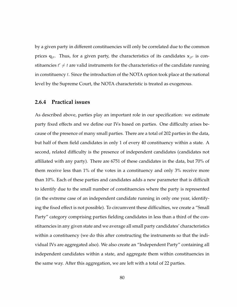
by a given party in different constituencies will only be correlated due to the common
prices qjt. Thus, for a given party, the characteristics of its candidates xjt′ is con-
stituencies t′ 6= t are valid instruments for the characteristics of the candidate running
in constituency t. Since the introduction of the NOTA option took place at the national
level by the Supreme Court, the NOTA characteristic is treated as exogenous.
2.6.4 Practical issues
As described above, parties play an important role in our specification: we estimate
party fixed effects and we define our IVs based on parties. One difficulty arises be-
cause of the presence of many small parties. There are a total of 202 parties in the data,
but half of them field candidates in only 1 of every 40 constituency within a state. A
second, related difficulty is the presence of independent candidates (candidates not
affiliated with any party). There are 6751 of these candidates in the data, but 70% of
them receive less than 1% of the votes in a constituency and only 3% receive more
than 10%. Each of these parties and candidates adds a new parameter that is difficult
to identify due to the small number of constituencies where the party is represented
(in the extreme case of an independent candidate running in only one year, identify-
ing the fixed effect is not possible). To circumvent these difficulties, we create a “Small
Party” category comprising parties fielding candidates in less than a third of the con-
stituencies in any given state and we average all small party candidates’ characteristics
within a constituency (we do this after constructing the instruments so that the indi-
vidual IVs are aggregated also). We also create an “Independent Party” containing all
independent candidates within a state, and aggregate them within constituencies in
the same way. After this aggregation, we are left with a total of 22 parties.
80

We include in the analysis the full list of candidate characteristics available in the
data: gender, caste, age and party. We select the constituency characteristics to be
included based on the variables that indicated significant heterogeneity in voter pref-
erences for NOTA in the regressions in section 2.5. We include percent male, literacy,
percent SC, percent ST, and the share of rural workers.
The BLP algorithm requires numerically solving the integral in (2.7) to obtain the
predicted market shares. We do this in the standard way by drawing individual voters
from the distribution of demographics in each constituency, computing the predicted
individual probabilities of voting for each candidate, and averaging across simula-
tions to obtain the simulator for the integral.
2.6.5 Results
Parameter estimates
We present parameter estimates for different specifications of the above model in Ta-
bles 2.7 and 2.8. First, we set Π and Σ equal to 0 so that voter heterogeneity only enters
through the εijt terms in equation (2.4). This is the conditional Logit model, and we
estimate it with and without instruments in columns (1) and (2) of Table 2.7. We report
coefficient estimates on the candidate characteristics as well as a subset of the control
variables (reserved constituency indicators and dummies for 3 major parties).
In column (3), we keep Π = 0 but allow for random coefficients on all the candi-
date characteristics as well as the outside option (through Σvi in equation (2.5) and σ0
in equation (2.6)). The estimates of Σ are in the first column of Table 2.8. Finally, we
present the full model which allows for both observed and unobserved heterogeneity
in voters’ evaluation of the various candidate characteristics. These estimates are in
81

column (4) of Table 2.7 (β) and the remainder of Table 2.8 (Σ and Π). Moving from col-
umn (1) to column (2) of Table 2.8, we kept those elements of Σ that were statistically
significant.
In Table 2.7, coefficients change substantially between the OLS and IV specifica-
tions, suggesting that instrumenting is important. Tables 2.7 and 2.8 reveal that voters
value candidate characteristics other than party affiliation. For example, older male
candidates tend to receive more votes. Allowing for taste heterogeneity among voters
regarding these characteristics in the full model substantially reduces the estimated
impact of party affiliation on votes (column (4) of Table 2.7). In Table 2.8, areas with
a higher share of ST voters yield more votes for ST candidates (this effect is identified
from variation across non-reserved constituencies). NOTA is a less popular option in
constituencies with more literate voters and in rural areas.
Counterfactual analysis: The impact of NOTA
In this section we use the estimated model to evaluate the impact of introducing
NOTA. We restrict attention to those constituencies in our data that had the NOTA
option available in 2013 and perform a counterfactual experiment where the NOTA
option is removed. We compute new vote shares and turnout rates under this coun-
terfactual scenario, and calculate the impact of NOTA as the difference between the
actual and the counterfactual outcomes.
The estimated impact of NOTA on turnout is shown in Figure 2.3. The average
increase in turnout is above 0.5 percentage points in 74% of the constituencies, with an
average of 1.2 percentage points. This is somewhat lower than the effect we obtained
82

from the reduced form exercise in section 2.5.2, but very close to the 1.4 percent of
eligible voters who voted for NOTA in the data.
The estimated impact of NOTA on individual candidates’ vote shares is shown
in Figure 2.4. The reduction in vote shares is smaller than 0.5 percentage points in
absolute value for 96% of the candidates, with a mean of 0.06 percentage points. This
indicates that substitution from voting for a candidate to voting for NOTA is minimal.
To gauge the impact of NOTA on parties, Table 2.9 aggregates voter choices by
party. For each party in the data, the first column gives the number of candidates and
the second column shows the fraction of the 101.2 million eligible voters who voted
for that party. The third column shows the difference relative to the counterfactual
without NOTA. For the two largest parties, BJP and INC, we estimate a loss in total
votes of around 0.15 percentage points. The change in the votes cast on other parties is
even smaller. By contrast the change in the overall abstention rate (and hence turnout)
is a magnitude larger at 1.2 percentage points. This is similar to the estimated effect
across all constituencies.
It should be emphasized that allowing for the flexible random coefficients spec-
ification above was crucial to obtain these results. The more restrictive Logit model
could not possibly have resulted in these effects. As is well known, the Logit specifica-
tion implies that substitution patterns only depend on observed choice shares. In our
case, this would imply that adding the NOTA option would, by construction, cause
the biggest change in the most popular candidate’s vote share. This is illustrated by
the last column of Table 2.9 which shows the counterfactual implications that would
be obtained from the Logit specification. As can be seen, this would imply that substi-
tution towards NOTA is similar for voters of the two largest parties and for abstaining
83
voters.
The patterns emerging from the demand model are similar to those observed in
the difference-in-differences analysis. The results indicate that NOTA votes are mostly
cast by voters who would have chosen to abstain in the counterfactual without NOTA
and turn out to vote specifically for NOTA. This provides strong evidence that voters
derive positive consumption utility from voting for this option.
2.7 Conclusion
This paper analyzed India’s NOTA policy which gives people the option to partici-
pate in elections and cast a valid “None of the Above” vote without the possibility of
affecting the electoral outcome. Individuals who choose to vote for NOTA but would
abstain otherwise must derive a consumption utility from voting that is specific to this
option. Thus, the NOTA policy makes it possible to test apart various components of
the consumption utility of voting. To address the challenge that, due to the secret bal-
lot, individual choices are not observable, we estimate counterfactual voter behavior
using a structural model and techniques borrowed from the consumer demand liter-
ature. The model allows for rich heterogeneity in voter preferences and relates these
parameters to the aggregate vote returns. In counterfactual simulations, we find that
the NOTA policy resulted in increased turnout. Based on the estimated model, vir-
tually all the NOTA votes observed in the data represent new voters who showed up
specifically to vote for NOTA and who would have abstained in the absence of this op-
tion. These patterns are also supported by the findings from a reduced-form analysis.
Our results show that, in this context, the presence of an option-specific consumption
84

utility from voting is necessary to explain the data. For example, voters may derive
utility from expressing their protest against one or more of the candidates running
for election. In this case, models that do not incorporate an option-specific utility of
voting would have a hard time explaining the data.
To the extent that voter participation is valuable in a democracy, our results suggest
that having a NOTA option on the ballot may be a desirable policy. It creates both
political participation and individual utility.
2.8 References
1. Ali, N., and C. Lin (2013): “Why People Vote: Ethical Motives and Social Incen-
tives,” American Economic Journal: Microeconomics
2. Bénabou, R. J., and J. Tirole. (2006). “Incentives and Prosocial Behavior,” Ameri-
can Economic Review
3. Berry, S., J. Levinsohn, and A. Pakes (1995): “Automobile Prices in Market Equi-
librium,” Econometrica, 63(4)
4. Besley, T., and S. Coate (1997): “An Economic Model of Representative Democ-
racy,” Quarterly Journal of Economics
5. Blais, A. (2000): To vote or not to vote, University of Pittsburgh Press, Pittsburgh,
PA.
6. Brennan, G., and L. Lomasky (1993): Democracy and Decision: The Pure Theory of
Electoral Preference. Cambridge University Press, Cambridge, UK.
85

7. Cameron, A.C., and D.L. Miller (2015): “A Practitioner’s Guide to Cluster-Robust
Inference,” Journal of Human Resources
8. Cantú, F., and O. García-Ponce (2015): “Partisan losers’ effects: Perceptions of
electoral integrity in Mexico,” Electoral Studies
9. Cho, W.K.T., and C.F. Manski (2008): “Cross-Level/Ecological Inference,” in:
J.M. Box-Steffensmeier, H.E. Brady, and D. Collier (eds.) The Oxford Handbook
of Political Methodology, Oxford University Press, Oxford, UK.
10. Coate, S. and M. Conlin (2004): “A Group Rule: Utilitarian Approach to Voter
Turnout: Theory and Evidence,” American Economic Review
11. Coate, S., M. Conlin, and A. Moro (2008): “The performance of pivotal-voter
models in small-scale elections: Evidence from Texas liquor referenda,” Journal
of Public Economics
12. Degan, A. and A. Merlo (2011): “A Structural Model of Turnout and Voting in
Multiple Elections,” Journal of the European Economic Association
13. DellaVigna, S., J.A. List, U. Malmendier, and G. Rao (2015): “Voting to Tell Oth-
ers,” working paper, UC Berkeley.
14. Dittmann, I., D. Kubler, E. Maug, and L. Mechtenberg (2014): “Why Votes Have
Value: Instrumental Voting with Overconfidence and Overestimation of Others’
Errors,” Games and Economic Behavior
15. Downs, A. (1957): An economic theory of democracy, Harper and Row, New York,
NY.
86

16. Driscoll, A., and M.J. Nelson (2014): “Ignorance or Opposition? Blank and
Spoiled Votes in Low-Information, Highly Politicized Environments,” Political
Research Quarterly
17. Duffy, J. and M. Tavits (2008): “Beliefs and Voting Decisions: A Test of the Pivotal
Voter Model,” American Journal of Political Science
18. Feddersen, T. and A. Sandorini (2006): “A Theory of Participation in Elections,”
American Economic Review
19. Fiorina, M. P. (1976): “The Voting Decision: Instrumental and Expressive As-
pects,” Journal of Politics
20. Glasgow, G., and R.M. Alvarez (2005): “Voting behavior and the electoral context
of government formation,” Electoral Studies
21. Greene, W.H. (2002): Econometric Analysis, Fifth Ed., Prentice Hall, Upper Saddle
River, NJ.
22. Harbaugh, W. T. (1996): “If People Vote Because They like to, then Why do so
Many of Them Lie?,” Public Choice
23. Hausman, J. (1996): “Valuation of New Goods Under Perfect and Imperfect
Competition,” in: T. Bresnahan and R. Gordon (eds.): The Economics of New Goods,
Studies in Income and Wealth Vol. 58, National Bureau of Economic Research,
Chicago, IL.
87

24. Herron, M. C. and J. S. Sekhon (2005): “Black Candidates and Black Voters: As-
sessing the Impact of Candidate Race on Uncounted Vote Rates,” Journal of Poli-
tics
25. McAllister, I. and T. Makkai (1993): “Institutions, Society or Protest? Explaining
Invalid Votes in Australian Elections,” Electoral Studies
26. McMillan, A. (2010): “The Election Commission,” in: N.G. Jayal and P.B. Mehta
(eds): The Oxford Companion to Politics in India, Oxford University Press, Oxford,
UK.
27. Nevo, A. (2000): “A Practitioner’s Guide to Estimation of Random Coefficients
Logit Models of Demand,” Journal of Economics and Management Strategy
28. Nevo, A. (2001): “Measuring Market Power in the Ready-to-Eat Cereal Indus-
try,” Econometrica
29. Ortoleva, P. and E. Snowberg (2015): “Overconfidence in Political Behavior,”
American Economic Review
30. Osborne, M., and A. Slivinski (1996): “A Model of Political Competition with
Citizen-Candidates,” Quarterly Journal of Economics
31. Petrin A. (2002): “Quantifying the Benefits of New Products: The Case of the
Minivan,” Journal of Political Economy
32. Power, T. J. and J. C. Garand (2007): “Determinants of invalid voting in Latin
America,” Electoral Studies
88

33. Razin, R. (2003): “Signaling and Election Motivations in a Voting Model with
Common Values and Responsive Candidates,” Econometrica
34. Rekkas, M. (2007): “The Impact of Campaign Spending on Votes in Multiparty
Elections,” Review of Economics and Statistics
35. Riker, H. W. and P. C. Ordeshook (1968): “A Theory of the Calculus of Voting,”
American Political Science Review
36. Selb, P., and S. Munzert (2013): “Voter overrepresentation, vote misreporting,
and turnout bias in postelection surveys,” Electoral Studies
37. Shachar, R., and B. Nalebuff (1999): “Follow the Leader: Theory and Evidence
on Political Participation,” American Economic Review
38. Shayo, M. and A. Harel (2012): “Non-consequentialist voting,” Journal of Eco-
nomic Behavior and Organization
39. Superti, C. (2015): “Vanguard of the Discontents: Blank and Null Voting as So-
phisticated Protest,” working paper, Harvard University.
40. Uggla, F. (2008): “Incompetence, Alienation, or Calculation? Explaining Levels
of Invalid Ballots and Extra-Parliamentary Votes,” Comparative Political Studies
41. Webb, M. (2013): “Reworking Wild Bootstrap Based Inference for Clustered Er-
rors,” working paper, University of Calgary.
89

2.9 Appendix
2.9.1 The correlates of NOTA votes
In this section we investigate the correlation between NOTA votes and constituency
characteristics. We use the same sample as in our structural exercise (the panel dataset
matched to the census data) and run simple cross-sectional regressions on the 520 con-
stituencies that are affected by the NOTA policy in 2013. We include state fixed effects
and, to avoid confounding our estimates by differential turnout across constituencies,
we measure NOTA vote shares as a fraction of total votes cast.29
The results are in Table 2.10. We find substantial heterogeneity in NOTA votes
across constituencies. For example, the NOTA vote share is significantly higher in re-
served constituencies and in constituencies with more illiterate voters, more women,
more ST, and a lower share of rural workers. Each of these patterns is consistent with
a variety of possible explanations. One possible interpretation is that NOTA votes are
higher in more economically disadvantaged populations, reflecting a general dissatis-
faction with elected leaders in these constituencies. Note however that the coefficients
remain unchanged if we add controls for various indicators of infrastructure and eco-
nomic activity in column (2). Another possible interpretation is that NOTA votes come
from politically underrepresented voters, such as women and non-SC or ST voters in
reserved constituencies.
In columns (3) and (4) we add candidate characteristics to the regression. These
estimates are merely suggestive because the list of candidates running will be affected
by their expected vote share, and this could be correlated with the fraction of voters
29Using NOTA votes as a share of eligible voters yields very similar results.
90

choosing NOTA. We find that constituencies with more candidates running result in
lower NOTA vote shares, which is consistent with NOTA reflecting dissatisfaction
with the menu of candidates being offered. We do not find evidence that the presence
of female, SC or ST candidates affects NOTA votes.
2.9.2 Robustness of the DD estimates
This section explores the robustness of the difference-in-difference estimates presented
in section 2.5.2 of the paper to various political events affecting one or more states.
National elections
In our study period, Indian national elections took place in Spring 2009 and 2014.
Recall that we do not include in the analysis the four states that hold their assembly
elections simultaneously with the national election. In the remaining states, because
split-ticket voting (constituencies voting for different parties at the state and national
levels) is common in India, it is ex ante not obvious that events affecting national
turnout, like the wave of support for the BJP in the 2014 national elections, would
affect assembly elections.30 If national elections did have an impact, we would expect
this to be the strongest for states that held assembly elections in October and December
of the national election years. If national elections impacted turnout in the assembly
elections in these states, this has the potential to confound our estimates of the NOTA
policy introduced between the two national election years in September 2013.
In Table 2.11 we exclude the national election years from the sample. Columns
(1) and (2) exclude 2014 and columns (3) and (4) exclude both 2009 and 2014. Odd30Note also that increased support for the BJP would lead to more BJP votes rather than NOTA votes.
91

numbered columns correspond to the specification in column (2) of Table 2.6 with the
basic controls and even numbered columns to column (3) with the extended controls.
We find that all point estimates are similar to, and if anything slightly larger than the
3 percentage points effect we found in Table 2.6. National elections do not appear to
confound the estimates reported in the main text.
Redistricting
Another potential confound is the electoral redistricting that took place in April 2008.
Because elections are held every 5 years and NOTA was introduced in September
2013, none of the states that were affected by NOTA in our period of study were re-
districted, while most states that were not affected by NOTA were redistricted. Thus,
redistricting has the potential to confound our estimates of NOTA.31
To control for this, we create a constituency-level measure of redistricting by us-
ing GIS boundary files to compare constituencies before and after the delimitation.
Our first measure calculates for each current constituency that was redistricted in
our study period the largest area that was part of a single constituency before the
redistricting. For example, a value of 0.8 for this “maximum overlap” measure indi-
cates that 80% of the current constituency’s area was part of a single constituency
pre-delimitation (while the remaining 20% was part of one or more different con-
stituencies). The higher the maximum overlap, the less a constituency was affected
by redistricting. Our second measure, rather than focus on the largest area of over-
lap, uses each overlapping area to create an index of “territorial fractionalization.” If
a constituency overlaps with n pre-delimitation constituencies with s1, ..., sn denoting
31For example, if redistricting lowered turnout, our estimate of NOTA’s effect of turnout would likelybe biased upward.
92

the share of its area falling in each of these, then the fractionalization index is 1−n∑i=1
s2i .
The larger this value, the more the current constituency was affected by redistricting.
Both of these measures are available for 22 states (constituency boundary files are not
available for the states of Assam, Manipur, and Nagaland).
Table 2.12 presents regressions corresponding to specifications (2) and (3) in Ta-
ble 2.6 controlling for these measures of redistricting. The first two columns repeat
columns (2) and (3) in Table 2.6 on the 22 states with available redistricting measures.
Columns (3) and (4) then add the maximum overlap measure and columns (5) and (6)
the territorial fractionalization index. As can be seen, adding either measure of redis-
tricting to the regressions causes very little change in the estimated effect of NOTA.
The estimates also retain their significance, except for column (6) where the standard
error increases just enough to yield a p-value of 0.101.32
State-specific events
Turning to state-specific events that may confound our estimates, we identified four
states where various events may plausibly affect 2013 or 2014 turnout relative to the
previous election (that is, turnout in the with-NOTA election relative to turnout in
the without-NOTA election). In Chhattisgarh, Maoist insurgents conducted terrorist
attacks in 2010 and May 2013, between the 2008 and 2013 elections in this state. In
Jammu & Kashmir, various incidents occurred between its 2008 and 2014 elections,
including a border skirmish in January 2013 between India and Pakistan described by
observers as one of the worst in 10 years. In Delhi, a new anti-corruption party, Aam
Aadmi entered politics in 2012, energized voters, and emerged as the second-largest
32The coefficients on the redistricting measures are never statistically significant.
93

party in the 2013 assembly election. Finally, Maharashtra held its 2009 election a year
after the 2008 terrorist attacks in Mumbai on several hotels and public buildings, and
security concerns may have depressed voter turnout there.
In Table 2.13, we repeat specifications (3) and (4) from Table 2.6 excluding each
of these states one at a time and then all four of them. The results corresponding
to the first specification are in column (1) and column (2) corresponds to the second
specification with the extended set of controls. All these coefficients are close to the
3 percentage point effect found in Table 2.6. The events in these four states do not
appear to drive the estimated effect of NOTA on turnout reported in the main text.
94

TABLE 2.1: Timeline of events in the study period
Year Month State assembly elections Other events2006 4 Assam
5 Kerala, Puducherry, Tamil Nadu,West Bengal
2007 2 Manipur, Punjab, Uttarakhand5 Uttar Pradesh6 Goa12 Gujarat, Himachal Pradesh
2008 2 Tripura3 Meghalaya, Nagaland4 Delimitation5 Karnataka11 Madhya Pradesh, NCT of Delhi12 Chhattisgarh, Jammu & Kashmir,
Mizoram, Rajasthan2009 4 Andhra Pradesh*, Arunachal Pradesh*, National elections
Odisha*, Sikkim*10 Haryana, Maharashtra12 Jharkhand
2010 10 Bihar*2011 4 Assam, Kerala, Puducherry, Tamil Nadu
5 West Bengal2012 1 Manipur, Punjab, Uttarakhand
3 Goa, Uttar Pradesh11 Himachal Pradesh12 Gujarat
2013 2 Meghalaya, Nagaland, Tripura5 Karnataka9 NOTA policy introduced11 Chhattisgarh, Madhya Pradesh12 Mizoram, NCT of Delhi, Rajasthan
2014 4 Andhra Pradesh*, Arunachal Pradesh*, National electionsOdisha*, Sikkim*
10 Haryana, Maharashtra12 Jammu & Kashmir, Jharkhand
Notes: * excluded from the dataset.
95

TABLE 2.2: Summary statistics of the electoral data at the constituencylevel
Variable Obs Mean Std. Dev. 10% 90%A. PanelNumber of candidates 1708 11.32 4.96 6 18Female candidates 1708 0.80 1.00 0 2Median candidate age 1708 44.07 5.45 38 51Eligible voters (1000) 1708 175.54 47.15 139.76 218.02Turnout 1708 0.71 0.09 0.58 0.82Winning vote share 1708 0.44 0.09 0.33 0.55NOTA votes / total votes 630 0.019 0.013 0.006 0.035NOTA votes / eligible voters 630 0.014 0.009 0.004 0.026Non-reserved constituencies:Number of SC candidates 1144 1.31 1.43 0 3Number of ST candidates 1144 0.48 1.04 0 2
B. Repeated cross sectionNumber of candidates 6685 10.54 5.35 5 17Female candidates 6685 0.73 0.97 0 2Median candidate age 6685 44.99 5.78 38 53Eligible voters (1000) 6685 180.75 88.23 41.20 292.90Turnout 6685 0.71 0.13 0.53 0.87Winning vote share 6685 0.45 0.10 0.32 0.56NOTA votes / total votes 1176 0.015 0.116 0.004 0.030NOTA votes / eligible voters 1176 0.010 0.009 0.003 0.022Non-reserved constituencies:Number of SC candidates 4842 1.24 1.56 0 3Number of ST candidates 4842 0.26 0.79 0 1Notes: The panel dataset contains the 2008 and 2013 state assembly elections in the states of Karnataka, NCTDelhi, Mizoram, Rajasthan, Madhya Pradesh, and Chhattisgarh. The repeated cross-section contains all assemblyelections between 2006 and 2014 in 25 states. Turnout is total votes divided by the number of eligible voters.Winning vote share is the winner’s share of all non-NOTA votes. Source: Election Commission of India.
96

TABLE 2.3: Candidate characteristics in the panel data
Variable All 2008 2013Age 44.42 43.98 44.87Female 6.87 6.87 6.88General caste 61.47 62.35 60.63SC 20.79 21.3 20.3ST 14.58 16.35 12.89Nationally recognized party 27.12 27.58 26.68State recognized party 3.89 4.9 2.93Other state-recognized party 8.05 6.9 9.15Unrecognized party 18.77 18.21 19.29Independent 39.01 42.41 35.76NOTA 3.16 - 6.18N 19957 9762 10195Notes: 2008 and 2013 state assembly elections in the states of Karnataka, NCTDelhi, Mizoram, Rajasthan, Madhya Pradesh, and Chhattisgarh. All numbersexcept Mean age are percentages. Source: Election Commission of India.
TABLE 2.4: Voter demographics at the state level (repeated cross-section)
Obs Mean Std. Dev. Min MaxLabor force participation 50 0.58 0.07 0.46 0.75Unemployment rate 50 0.02 0.03 0.00 0.15Real household earnings (Rp per week) 50 1708 665 864 4335Fraction illiterate 50 0.25 0.13 0.04 0.52Fraction primary school or less 50 0.23 0.09 0.13 0.53Female per 1000 male 50 987 72 790 1172Fraction urban 50 0.32 0.18 0.09 0.97State NDP growth rate 50 6.11 4.57 -5.38 24.31Notes: Source for all variables except NDP growth rate: National Sample Survey, rounds 62, 64, 66,68, 71. Individual surveys for respondents above 18 were aggregated to the state level. Householdearnings deflated to 2001 prices using the CPI from the Reserve Bank of India. Source for NDPgrowth rate: Reserve Bank of India.
97

TABLE 2.5: Demographic characteristics of the constituencies from theIndian Census (panel dataset)
Variable Mean Std. Dev. 10% 90%Literate 0.58 0.09 0.47 0.69Percent male 0.51 0.01 0.50 0.53Percent SC 0.18 0.07 0.08 0.26Percent ST 0.29 0.18 0.16 0.58Percent employed 0.46 0.05 0.40 0.52Percent rural workers 0.66 0.17 0.44 0.84Fraction of households with infrastructure:No latrine 0.71 0.22 0.37 0.91Water near premises 0.47 0.10 0.35 0.59Water on premises 0.26 0.16 0.10 0.47Fraction of households owning asset:Car 0.03 0.02 0.01 0.06Computer 0.01 0.01 0.002 0.02Phone 0.55 0.20 0.25 0.78TV 0.37 0.17 0.15 0.61Notes: Source: Indian Census, 2011. Village level census data was merged to assemblyconstituency GIS boundary files as described in the text. N = 723.
98

TABLE 2.6: The impact of NOTA on turnout, DD estimates
(1) (2) (3)NOTA 0.035 0.029** 0.030*s.e. (0.013) (0.016)bootstrap p-value [0.587] [0.036] [0.060]Eligible voters, labor force participation, x x xhh earnings, educationPolitical reservation, unemployment, sex xratio, urbanization, NDP growth rateConstituency FE xState FE x xR2 0.78 0.18 0.19N 1708 6685 6685States 6 25 25Notes: Estimates of the effect of the NOTA policy on turnout from Eqn. (2). All regressions control for time fixedeffects, the log number of eligible voters in a constituency and its square, and the following state-level variables:labor force participation, real weekly household earnings, fraction of illiterates, fraction with primary schoolor less as highest education. Column (3) also controls for reserved constituencies and the following state levelvariables: unemployment, sex ratio, fraction urban, and the growth rate of net domestic state product. Standarderrors clustered by state in parentheses. The bootstrap p-value was computed using a wild bootstrap procedurewith a 6-point weight distribution. ***, **, and * indicate significance at 1, 5, and 10 percent, respectively.
99

TABLE 2.7: Estimates of the linear parameters of the demand system
InstrumentalVariable Random
OLS Logit Logit Coefficients Full modelVariable (1) (2) (3) (4)Female -0.090** -0.153 -1.547* -3.725
(0.044) (0.268) (0.928) (2.992)Age 1.029*** 8.925*** 8.013*** 10.231*
(0.116) (1.423) (2.097) (5.767)SC candidate -0.370*** 0.273 0.377 0.120
(0.047) (0.223) (0.385) (1.266)ST candidate -0.043 0.082 0.143 2.002
(0.067) (0.148) (0.386) (2.878)NOTA 0.269*** -3.439*** -4.263*** -61.830***
(0.074) (0.076) (0.890) (11.052)Reserved SC 0.302*** -0.202 -0.258 -0.140
(0.048) (0.189) (0.360) (0.954)Reserved ST 0.290*** 0.351*** 0.734*** -1.923
(0.064) (0.115) (0.194) (2.688)Party: BJP 2.664*** -5.135*** -4.677*** -1.994
(0.042) (0.728) (0.990) (3.104)Party: INC 2.738*** -5.157*** -4.724*** -2.089
(0.041) (0.745) (1.017) (3.177)Party: BSP 0.325*** -7.039*** -6.802*** -4.348
(0.045) (0.644) (0.895) (2.933)Notes: The table reports estimates of the linear parameters of the model (β). All specifications include afull set of party dummies (three of which are reported in the table) as well as dummies for states, years,and constituency reservation status. Columns (2)-(4) include instrumental variables as described in thetext. Robust standard errors in parentheses. ***, **, and * indicates significance at 1, 5, and 10 percent,respectively.
100

TAB
LE
2.8:
Esti
mat
esof
the
nonl
inea
rpa
ram
eter
sof
the
full
mod
el
Stan
dard
Stan
dard
Dev
iati
ons
Dev
iati
ons
Inte
ract
ions
wit
hD
emog
raph
icV
aria
bles
Var
iabl
e(1
)(2
)Pe
rcen
tSC
Perc
entS
TPe
rcen
tmal
eLi
tera
cyR
ural
Fem
ale
-3.8
73**
-7.0
81*
--
6.21
4-
-(1
.513
)(3
.813
)(6
.498
)A
ge-0
.915
--
--
--
(2.4
53)
SCca
ndid
ate
0.00
3-
0.06
0-
--
-(1
.799
)(2
.188
)ST
cand
idat
e1.
951*
*4.
971*
**-
6.45
2*-
--
(0.8
59)
(1.7
08)
(3.5
56)
NO
TA1.
343
--
-43.
704
-42.
581
-45.
274*
-24.
270*
*(0
.839
)(4
3.32
2)(3
4.23
1)(2
4.27
6)(1
1.30
5)C
onst
ant
-0.0
60-
--
-13
.066
***
6.08
2***
(1.6
50)
(1.8
81)
(1.9
27)
Not
es:
The
tabl
ere
port
ses
tim
ates
ofth
eno
nlin
ear
para
met
ers
ofth
em
odel
(Πan
dΣ
).’S
tand
ard
devi
atio
ns’r
efer
toth
eΣ
para
met
ers
ofth
era
ndom
coef
ficie
nts.
The
spec
ifica
tion
inco
lum
n(1
)co
rres
pond
sto
colu
mn
(3)
inTa
ble
7an
dre
stri
cts
Π=
0.
The
rem
aini
ngco
lum
nsof
the
tabl
eco
rres
pond
toth
esp
ecifi
cati
onin
colu
mn
(4)i
nTa
ble
7.R
obus
tsta
ndar
der
rors
inpa
rent
hese
s.**
*,**
,and
*in
dica
tes
sign
ifica
nce
at1,
5,an
d10
perc
ent,
resp
ecti
vely
.
101

FIGURE 2.1: Constituencies in the merged dataset
102

TABLE 2.9: Impact of NOTA on vote shares by party
Change with NOTAN. of Percent of
Party candidates all voters Full model LogitBJP 506 32.90 -0.17 -0.63BSP 498 3.63 -0.02 -0.09BYS 102 0.10 0.00 -0.01CSM 54 0.22 0.00 -0.01GGP 44 0.20 0.00 -0.01INC 518 26.74 -0.14 -0.58Independents 468 4.96 -0.03 -0.11JGP 85 0.06 0.00 0.00MNF 10 0.06 0.00 0.00NPEP 133 1.30 -0.01 -0.02SP 194 0.43 0.00 -0.01ZNP 11 0.02 0.00 0.00Small Party 445 2.70 -0.01 -0.05Abstention 25.11 -1.20 -0.76Notes: The table shows, for each party, the total number of candidates and the correspond-ing share of all voters in the data (out of 101.168 million eligible voters). The last twocolumns are the simulated effects of introducing NOTA in the full random coefficientsspecification as well as in the more restrictive Logit model.
103

TABLE 2.10: The correlates of NOTA votes
(1) (2) (3) (4)Constituency characteristics:Reserved SC 0.005*** 0.005*** 0.002** 0.002**
(0.001) (0.001) (0.001) (0.001)Reserved ST 0.011*** 0.011*** 0.009*** 0.009***
(0.002) (0.001) (0.002) (0.002)Literacy -0.021*** -0.035*** -0.015** -0.026**
(0.006) (0.010) (0.006) (0.010)Size -0.006* -0.008** -0.003 -0.005
(0.003) (0.004) (0.003) (0.004)Percent male -0.215*** -0.230*** -0.133*** -0.190***
(0.031) (0.046) (0.033) (0.043)Percent SC 0.002 0.010 -0.006 0.006
(0.008) (0.009) (0.007) (0.008)Percent ST 0.010*** 0.008* 0.010** 0.007
(0.004) (0.004) (0.004) (0.004)No latrine 0.002 0.004
(0.004) (0.004)Water nearby 0.016** 0.014**
(0.006) (0.006)Water at home 0.011* 0.013**
(0.006) (0.005)Percent employed 0.015 -0.004
(0.011) (0.011)Rural workers -0.019*** -0.015***
(0.005) (0.005)Car ownership 0.023 0.020
(0.037) (0.034)Computer ownership -0.029 0.036
(0.057) (0.052)Phone ownership -0.009 -0.010*
(0.006) (0.005)TV ownership -0.003 -0.007
(0.006) (0.006)Candidate characteristics:Number of candidates -0.001*** -0.001***
(0.000) (0.000)No female -0.001 -0.001
(0.001) (0.001)<15% female -0.000 -0.000
(0.001) (0.001)Median age -0.000 -0.000
(0.000) (0.000)No SC 0.000 -0.000
(0.001) (0.001)<15% SC -0.000 0.000
(0.001) (0.001)No ST -0.000 -0.000
(0.001) (0.001)<10% ST 0.002 0.001
(0.001) (0.002)R2 0.57 0.60 0.63 0.66N 520 520 520 520Notes: The dependent variable is the share of NOTA votes among all votes. Regressions at the con-stituency level for the cross-section of constituencies affected by the NOTA policy in 2013. Mergeddataset: average demographic characteristics are from the census, average candidate characteris-tics are from the Election Commission. All regressions include state fixed effects. Robust standarderrors in parentheses. ***, **, and * indicates significance at 1, 5, and 10 percent, respectively.
104

TABLE 2.11: Effect of NOTA on turnout, excluding national election years
(1) (2) (3) (4)NOTA 0.033** 0.033** 0.030* 0.031*
(0.015) (0.016) (0.015) (0.015)Basic controls x xExtended controls x xExcluded years 2014 2014 2009, 2014 2009, 2014R2 0.18 0.20 0.19 0.21N 6139 6139 5680 5680States 25 25 22 22Notes: Estimates of the effect of the NOTA policy on turnout from Eqn. (2) using the repeatedcross section sample with specific years excluded. All regressions control for state and yearfixed effects, the log number of eligible voters in a constituency and its square, and the follow-ing state-level variables: labor force participation, real weekly household earnings, fractionof illiterates, fraction with primary school or less as highest education. The Extended controlsspecification also controls for reserved constituencies and the following state level variables:unemployment, sex ratio, fraction urban, and the growth rate of net domestic state product.Standard errors clustered by state in parentheses. ***, **, and * indicate significance at 1, 5,and 10 percent, respectively.
TABLE 2.12: Effect of NOTA on turnout, controlling for redistricting
(1) (2) (3) (4) (5) (6)NOTA 0.033** 0.022* 0.031** 0.020* 0.030** 0.020
(0.016) (0.011) (0.015) (0.011) (0.014) (0.012)Basic controls x x xExtended controls x x xR2 0.21 0.23 0.21 0.23 0.21 0.23N 6084 6084 6084 6084 6084 6084States 22 22 22 22 22 22Notes: Estimates of the effect of the NOTA policy on turnout from Eqn. (2) using the repeated cross section sam-ple. Columns (1) and (2) are run on the states with available constituency boundary files. Columns (3) and (4)control for redistricting using the maximum overlap measure and columns (5) and (6) using the territorial frac-tionalization index. All regressions control for state and year fixed effects, the log number of eligible voters in aconstituency and its square, and the following state-level variables: labor force participation, real weekly house-hold earnings, fraction of illiterates, fraction with primary school or less as highest education. Even-numberedcolumns also control for reserved constituencies and the following state level variables: unemployment, sex ratio,fraction urban, and the growth rate of net domestic state product. Standard errors clustered by state in parenthe-ses. ***, **, and * indicate significance at 1, 5, and 10 percent, respectively.
105

TABLE 2.13: Effect of NOTA on turnout, robustness to state-specificevents
Excluded state Effect of NOTA NBasic controls Extended controls
Chhattisgarh 0.025* 0.035 6505(0.014) (0.021)
Maharashtra 0.031** 0.031* 6109(0.015) (0.015)
Delhi 0.029** 0.031* 6545(0.013) (0.016)
Jammu and Kashmir 0.030** 0.031* 6511(0.014) (0.016)
All four 0.028* 0.039* 5615(0.015) (0.019)
Notes: Estimates of the effect of the NOTA policy on turnout from Eqn. (2) using the repeated crosssection sample with specific states excluded. All regressions control for state and year fixed effects, thelog number of eligible voters in a constituency and its square, and the following state-level variables: laborforce participation, real weekly household earnings, fraction of illiterates, fraction with primary school orless as highest education. The Extended controls specification also controls for reserved constituenciesand the following state level variables: unemployment, sex ratio, fraction urban, and the growth rateof net domestic state product. Standard errors clustered by state in parentheses. ***, **, and * indicatesignificance at 1, 5, and 10 percent, respectively.
106

FIGURE 2.2: Distribution of NOTA vote shares across constituencies
Notes: NOTA vote share is measured as a fraction of total votes cast. N = 1176.
107

FIGURE 2.3: Impact of NOTA on turnout
Notes: Distribution of the changes in turnout across constituencies. Mean = 0.0119, median = 0.0100, N= 519.
108

FIGURE 2.4: Impact of NOTA on candidates’ vote shares
Notes: Distribution of the changes in vote shares across candidates. Mean = -0.0006, median = -0.0000,N = 3068.
109

110
Chapter 3
Firm Ownership and Wage Dispersion:
Evidence from Ghana Using Matched
Employer Employee Data
3.1 Introduction
The role of the firm in worker wage dispersion has been little studied empirically.
It is however considered as a very important determinant of wage inequality. The
environment in which a worker is working may have direct and indirect consequences
on his eventual earnings through measured or unmeasured channels. The idea of
unmeasured worker ability on the one hand and pure industry or firm effects on the
other hand are believed to be important factors affecting observed wage dispersion.
Existing empirical work has shown that neither of these explanations can be re-
jected but seperately identifying these effects using longitudinal data is difficult. As
Hamermesh (2008) points out, the effect would be overstated in favor of the group
on which more information is available. So, if information on workers is richer than

that on firms, the estimated effect of workers would look a lot bigger than that of
firms and vice-versa. This is more of a concern if we believe that the worker and
firm characteristics are correlated. Hamermesh notes that it is much better if we have
a matched employer-employee dataset. In this paper, I use matched data from the
Ghanaian manufacturing industry to analyze the role of firms in observed wage dis-
persion among workers. The empirical methodology of this paper closely follows
Barth et al (2014).
Barth et al (2014) is, to the best of my knowledge, the only paper that studies the
role of establishments in explaining wage inequality using US data. I apply their
methodology to study the same question in a developing country setting. Addition-
ally, I look at how patterns of inequality vary by firm ownership type. Specifically,
are private firms owned domestically different from foreign owned firms? Are the
firm effects explaining wage dispersion different based on ownership structure? I also
analyze how trends in earnings dispersion differ by worker skills.
In the Ghanaian manufacturing sector, we see majority of the manufacturing firms
in the private sector. 1This is largely due to the extensive economic reforms that have
been implemented since the mid to late 1980s. This paper also contributes to the litera-
ture in terms of analyzing earnings in the post-reform era in Ghana. I find an unusual
and very interesting pattern of wage inequality in the Ghanaian manufacturing sector
in this period. In the early period, as the reforms were perhaps sinking in, the vari-
ance in worker earnings increased but towards the end of the 1990s, by the time the
reforms had potentially taken full effect, the variance in earnings actually decreased.
However, while this pattern is true for domestic private firms in Ghana, firms with
1This is true in terms of the dataset I use. Census figures may be different nonetheless.
111

other types of ownership did not witness this decline in the later periods and they ex-
perience a secular increase in variance of earnings. Much of this paper is focussed on
analyzing this interesting pattern and estimating what role the firm component might
have played in this.
Analyzing the variance components, I find that this pattern is explained mainly
by fluctuations in the between-firm variation. The variation within-firms has been
steadily increasing. The initial rise in variance and the later fall seems to be due to
variation between firms rather than within firms. It is important to understand if this
pattern can be explained by gains and losses made by the workers at the top of the
earnings distribution. Interestingly, I find that while net gains to workers above the
90th percentile can explain about 61% of the initial surge in variance, it only explains
about 9% of the later fall. This suggests that workers below the 90th percentile must
have made significant gains in the later stages which resulted in closing down of the
earnings gap. This can possibly be attributed to economic reforms, though the empir-
ical analysis of this paper cannot identify if this is a pure causal effect or not.
I further analyze the interaction of worker and firm characteristics in a regression
setting and find that the variance in workers’ predicted wage from observable charac-
teristics have increased over time whereas the variance of the firms’ effect on wages
have declined over time. This pattern is observed for the average firm and on av-
erage for firms owned privately by domestic Ghanaians. For foreign owned firms
however, this is not replicated. The data suggests that the inverted u-shaped pattern
of variances of log real hourly earnings for private firms can mostly be explained by a
decline in the firm specific effect at the latter stages. The correlation between the con-
tribution of individual attributes to wages and the firm effect have declined over time.
112

This suggests that firms have gradually hired workers by observable characteristics,
independent of firm specific earnings, or in other words, their preference towards hir-
ing similar workers within a firm has decreased. I find that for high skilled workers,
inequality increases over time whereas it declines for low skilled workers.
The rest of the paper is organized as follows. Section 2 gives some background in-
formation. The empirical methodology is introduced in Section 3 and Data in Section
4. The main results are in Section 5. In Section 6, I briefly discuss how the estimated
effects are different over time periods and present conclusions in Section 7.
3.2 Background
3.2.1 The Ghanaian Manufacturing Sector
The Ghanaian economy went through economic reforms from 1983-1991. The manu-
facturing sector was believed to be the engine through which employment generation
and long term economic growth would be attained. (See Teal 1998). An immediate
consequence of providing impetus to the manufacturing sector is that demand for
skilled labor would rise. This was no different for Ghana particularly because the two
most flourishing manufacturing sectors in Ghana were wood products and textiles.
Detailed review of the impact of reforms on the Ghanaian economy can be found in
Baah-Nuakoh and Teal (1993). The manufacturing sector has contributed consistently
113

to around 8-10% of the GDP of Ghana ever since the reforms. Even though by stan-
dards expected by the reform, this may look like a small number but the sector em-
ploys over 250,000 people. 2 Apart from wood and textiles, food processing, smelting,
oil refining, cement and pharmaceuticals are other important sectors in manufactur-
ing in Ghana. A rising concern for the sector is the influx of cheap goods from other
economies like China which have massive comparative advantages in manufacturing.
This is not just a concern for the Ghanaian economy but most of the western African
nations. A recent study by Szabo (2014) points out the inefficiencies in the manufac-
turing sector of Ghana. Szabo estimates production functions for the manufacturing
firms and finds that firms mostly use more capital and less labor than the optimal
amount.
In the wake of this situation, it is worthwhile to look at the wage patterns in the
Ghanaian manufacturing sector which has been the center of attention for Ghanaian
policymakers. It remains indeterminate whether the sector has given the economy
the necessary fillip towards economic growth but we can see how much wages have
changed over time in this sector post the reforms and whether the pre dominance
of private owenrship has had significant effects on worker wages or not. Existing
research has pointed out that there is a link between economic growth and wage dis-
persion in African economies (see Agesa et al, 2011 for details in the context of Kenya).
2See Natcomm Report on Ghanaian Manufacturing Sector -http://www.natcomreport.com/ghana/livre/manufacturing.pdf
114

3.2.2 Related Literature and Conceptual Framework
The study of wage dispersion using matched employer employee datasets has gained
popularity in the last decade and a half. Abowd, Kramarz and Margolis (1999) in
their seminal paper introduced the use of a linked employer employee data set to run
a additively separable fixed effects framework using French data to disentangle the
true effect of a firm from that of the worker.
Fafchamps, Soderbom and Benhassine (2008) studied the African manufacturing
sector and analyzed the role of sorting in explaining wage gaps. Not much is known
however in terms of the role of firms in explaining dispersion in such poor countries.
This paper is an attempt to fill this void in the literature. To my knowledge, this is the
first paper to use a matched employer employee dataset to look at wage dispersion by
ownership pattern for a developing country. In particular the idea is to see if private
domestic ownership of firms leads to higher or lower wage dispersion as compared to
other types of ownership like state-owned, foreign or mixed.
The effect of unobserved worker ability and firm components on wage dispersion
maybe very different for firms owned and managed differently. Especially after eco-
nomic reforms, one might expect more FDI to flow in and more foreign firms being
setup. A body of literature analyzes the impact of FDI inflows on wage dispersion
(Saglam and Sayek, 2011; Heyman, Sjoholm and Tingvall, 2011; Almeida, 2007 and
Martins, 2004). The findings generally indicate that foreign firms lead to higher wage
dispersion and also pay higher actual wages. One explanation is that foreign owned
firms hire skilled workers and that leads to dispersion. Also, lower skilled workers
sort to other firms and hence inter- as well as intra-firm dispersion rises.
It is therefore important to understand if firm behavior actually explains more of
115

the dispersion in wages when owned by foreign enterprises. The following empiri-
cal exercise is an attempt to answer this question. If foreign ownership indeed leads
to higher dispersion, then the firm component should explain more of the wage dis-
persion than worker components. Also, if domestic firms are selected by low skilled
workers, then worker components should explain dispersion more than firm effects
for such firms.
3.3 Empirical Methodology
3.3.1 Analyis of Variance
The empirical strategy I adopt is largely descriptive but provides valuable insight. I do
a variance decomposition of log real hourly earnings into within-firm and between-
firm elements. The matched component of my dataset facilitates this exercise. I follow
the method of Barth et al (2014) throughout this paper and analyze the variance com-
ponents as follows:
V ar(lnwif ) = V ar(Elnwif ) + V ar(lnwif − Elnwif ) (3.1)
where lnwif is the log real hourly earnings (before taxes) for individual ‘i’ working at
firm ‘f’. Elnwif represents the expected value of earnings of workers working at firm
‘f’. V ar(Elnwif ) is the between-firm variance and V ar(lnwif − Elnwif ) is the within
firm variance.
116

3.3.2 Percentile Analysis: Contribution of Earnings Gap to Variance
Barth et al (2014) also propose an arithmetic decomposition of the variance in log real
earnings to calculate the contribution of the difference in mean earnings for various
groups of individuals on the actual variance based on the percentile distribution of
earnings. Suppose we want to compare individuals above the p-th percentile to those
below the p-th percentile. Then if E(p) is the mean of log real hourly earnings of the
top p% and E(100−p) is the mean log real hourly earnings for the remaining workers,
then the variance can be decomposed as follows:
V ar(lnw) =p
100·100− p
100·[E(p)−E(100−p)]2+
p
100·V ar(p)+100− p
100·V ar(100−p) (3.2)
For this paper, I will focus on the earnings gap at the 90th percentile. So the above
reduces to:
V ar(lnw) = (0.1) · (0.9) · [E(10)− E(90)]2 + (0.1) · V ar(10) + (0.9) · V ar(90) (3.3)
The contribution of the earnings gap to variances is therefore given by the term
(0.1) · (0.9) · [E(10)− E(90)]2.
3.3.3 Worker Characteristics and Firm Fixed Effects
The third and final strategy of this paper is to run a modified Mincerian regression for
time periods ‘t’ as follows:
117

lnwif = β.Xif + δf + uif (3.4)
The vectorXif includes worker characteristics like hours worked, age, age squared,
experience, experience squared, education, education squared, parents’ experience
and parents’ experience squared for worker i in firm f . Using the methodology de-
scribed in Barth et al (2014), I decompose the variance of (4) as follows:
V ar(lnw) = V ar(κ) + V ar(δ) + 2cov(κ, δ) + V ar(u) (3.5)
In the above, κ = X · β and represents the predicted earnings from observable
worker characteristics. The term V ar(δ) represents the variance of earnings among
firms or the variance of the firm fixed effects. Another statistic of interest is the degree
of how similar workers are within a given firm, ρδ = cov(κ,δ)V ar(κ)
. Barth et al (2014) note
that if ρδ is close to zero, firms are independently hiring workers based on observed
characteristics, independent of firm earnings.
3.4 Data
The dataset for this study is a panel survey of the Ghanaian manufacturing sector
which took place from 1992 to 2003. The survey was the joint venture of Center
for Study of African Economies (CSAE), the University of Oxford, the University of
Ghana, Legon and the Ghana Statistical Office for the Regional Project for Enterprise
Development (RPED) and Ghana Manufacturing Enterprise Survey. The original sam-
ple of firms was drawn randomly from the 1987 census of manufacturing activities of
118

Ghana. From each of the firms a sample of workers were also interviewed in this pe-
riod. This allows matching the two databases to form a linked employer-employee
dataset. 3
Figure 3.1 shows the shares of firms by ownership categories from our sample. It
appears that the majority of firms are privately owned but some have foreign owner-
ship. For the eventual empirical analysis, I am going to break down the sample into
firms owned and managed by private Ghanaian agents, viz, Private Domestic Firms
and firms with some foreign ownership. The latter would include firms partially or
wholly owned by foreign owners. The remainder of the firms are state owned. Table
3.1 shows some descriptive statistics from plant level data. Column (1) reports means
for all firms whereas columns (2) and (3) report means for the other two categories.
All the means are averages across 12 years of data. Figure 3.2 gives the time series
plots of plant level averages of some of these observables by ownership types.
The average firm has about 75 workers whereas this number is much smaller for
private domestic firms (34) and much higher for foreign owned firms (194). The num-
ber of skilled workers as identified by the firms in their responses to the survey ques-
tion is 14 on average for the whole sample whereas for private domestic it is much
smaller at around 7 skilled workers per firm. The average education of workers is
about 10 years across firm types. Foreign owned firms seem to have workers with
higher average age and potential experience compared to the overall average. Most
foreign owned firms are located in the capital city of Accra. I also find that foreign
firms are more likely to export goods compared to private domestic firms. Value of
3The survey yields a dataset which is a balanced panel of 200 firms but a repeated cross section ofworkers. It was conducted over 7 rounds. The first three rounds were annual surveys, the next threecovered two years each and the last covered three years.
119

total output is higher for foreign firms throughout the span of the data.
There is not much difference in the hours worked by the average worker in these
firms although it is slightly less for foreign owned firms. Foreign owned firms also
have higher wage bills. In terms of input usage and capital, the data suggests that on
average 22% of the inputs are imported. This number is somewhat smaller at under
20% for private domestic firms but significantly higher at 33% for foreign owned firms.
In terms of replacement value of plant and machinery, the mean for foreign firms is
above the average and that for private domestic is below the average for all firms.
3.5 Results
3.5.1 Within-Firm and Between-Firm Effects
Figure 3.3 is indicative of how log real hourly earnings varied in Ghana over the years
(1992-2003). A striking feature of this graph is that the variance of earnings seem to re-
semble an inverted u-shape for Ghanaian manufacturing firms. The variances seem to
have increased from 1992 to around 1998 after which the variances show a decline in
trend. This is intriguing because unlike secular increases in earnings inequality which
are common in the developed world, including the US, here I observe a decline after
an initial surge. . One possible reason for this pattern in the Ghanaian manufacturing
sector is the reforms that happened extensively in the late 80s and continued into the
early 90s. It is plausible that the effects of the reforms on the manufacturing sector,
especially for the domestic firms started accruing around the mid nineties. This might
be the reason that earnings inequality appears to have been checked since 1998 and
into the 2000s. A feature of the Ghanaian manufacturing sector was overstaffing. It is
120

believed that post-reform this has reduced a lot.4 This may have also contributed to
paying workers more efficiently and a resultant decline in earnings inequality. In Fig-
ure 3.3, I look at composition of this variance changes for different ownership patterns.
The Ghanaian manufacturing sector is dominated by private firms. So, I restrict my
analysis only to such firms and find that the inverted u-shaped pattern is replicated
only for domestic firms and not for the foreign owned firms.
The rest of this paper delves deeper into this phenomenon and attempts to analyze
the components underlying such patterns of dispersion. The preceeding discussion
first leads us into the following question: are these patterns due to within-firm or
between-firm variation in worker earnings and how do changes in these components
reconcile the overall trends in dispersion? To answer this question, I decompose the
variances following equation 3.1. The results are reported in Table 3.2. I report the total
variance of log real hourly earnings along with the within and between components
for 3 different years,viz, 1992, 1998 and 2003 to illustrate how the change in overall
variances compare to the change in the within and between components. I find that
for all firms, the within-firm variation has increased over time from 0.444 in 1992 to
0.514 in 1998 and 0.748 in 2003. However, the inverted u-shape of the total variance
curve can be explained mainly by the between-firm component of earnings. I find that
in the early period, the between firm component rises from 0.661 to 0.862 but it falls
to 0.319 in the latter half. This suggests that the between firm component seems to
explain the pattern that we observe in the dispersion of earnings.
Looking at changes over time, I find that the total variance increased in the early
period and declined in the latter by a larger magnitude. The change in within variation
4See Ackah, Adjasi and Turkson - http : //www.brookings.edu/ /media/Research/F iles/Papers/2014/11/learning−to− compete/L2CWP18Ackah−Adjasi− and− Turkson.pdf?la = en
121

increased. So what drives this decline is likely to be the change in between variation.
I find that the change in between-firm variance declined from 0.201 to -0.541.
In Table 3.3, I analyze the overall variances in earnings by firm type. There are
some interesting patterns to note. For private domestic firms, variance seems to be
initially flat but declines in the latter period whereas for private foreign firms it seems
to increase in the early period and remain stable in the latter period. If an influx of
foreign investment disproprotionately attracts skilled labor, this may lead to rising
inequality in the other sectior, viz, domestic in our case.5
3.5.2 Percentile Analysis
Given that we observe the inverted u-shaped pattern for variances in log real hourly
earnings, the question of gainers versus losers assumes importance. The purpose of
this exercise is to estimate whether gains to the workers at the top of the earnigns
distribution has contributed to the inequality? For our unique case, this question can
be reframed to accomodate the decline in inequality at the latter stages to see if top
earners have lost out on the gains they made or have the rest of the workers caught
up. I perform the empirical analysis described in the empirical methodology section
above and focus on the decomposition as per equation 3.3.
Table 3.4 presents the relevant results. I break up the analysis into two periods
of time. The surge phase (1992-1998) and the decline phase (1998-2003). In Panel A,
I analyze the surge phase. Column 2 reports statistics from 1992, column 3 reports
5 To investigate this further, I looked at the variances by worker skill and found that the inequalityfor low skilled workers has reduced over time consistently. This is indicative of the fact that as skilledworkers sort into foreign firms, the unskilled (or low skilled) workers end up in domestic firms anddomestic firms have a lower skilled pool to choose from. This may lead to a decline in dispersion forlow skilled workers.
122

statistics from 1998 and column 4 reports the changes from 1992-1998. I find that the
variance of log real hourly earnings increased by 0.271 log points from 1.105 in 1992
to 1.376 in 1998. I calculate the means of log real hourly earnings for two sets of
workers, viz, above the 90th percentile and below the 90th percentile. I find that in
1992, the difference in these means was 1.649 and it increased to 2.138 in 1998. Using
the expression in equation 3.3, I calculate the contribution of these mean differences
to the variance in earnings.
In 1992, the difference in mean log real hourly earnings for workers above and
below the 90th percentile contributed 0.245 log points of the total variation of 1.105.
This number increased to 0.411 in 1998. The increased contribution of these differences
was 0.166 over the surge period which accounts for 61.25% of the total increase in
variance during this time period. This suggests that the increased advantage of the
top earners over the rest had a major contribution to the surge in wage dispersion in
Ghana during 1992-1998.
I replicate the above analysis for the decline phase and report the statistics in Panel
B. Variance in log real hourly earnings declined from 1.376 in 1998 to 1.067 in 2003,
a change of 0.309 log points. The difference in means of log real hourly earnings for
workers above and below the 90th percentile decreased from 2.138 in 1998 to 2.062
in 2003. The contribution to the overall variance changed by 0.028 which is approx-
imately 9.06% of the total decline in variance. So the relative advantage of the top
earners was not entirely wiped out and was not the major reason why the surge in
inequality reversed. This suggests that workers in the rest of the distribtuion of earn-
ings made significant gains in the latter phases which could probably be attributed to
the sinking in of economic reforms.
123

3.5.3 Returns to Schooling and Earnings Dispersion
I run simple Mincerian regressions as described by equation 3.4 with X denoting the
observables like years of schooling, experience and experience squared only. I use
firm fixed effects and run these regressions for two periods of time, 1992-1998 and
1998-2003. OLS estimates of the coefficients are reported in Table 3.5. I find that the
returns to schooling increased over time whereas the marginal effect of experience
seems to have declined over time. Variance of the predicted earnings from education
and experience has increased from 0.109 to 0.133. This is not consistent with the fall in
variance of earnings over time suggesting that the decline in inequality is explained
more by firm factors and residuals and not necessarily by a decline in inequality of
returns to schooling and experience.
3.5.4 Does Predicted Wage Dispersion by Worker and Firm Charac-
teristics Vary by Ownership Structure?
This is the final section of the empirical analysis and I run the regression described
by equation 3.4 using all observable worker characterisitcs as controls. Since I have
identified two distinctive time periods in the data for studying variance in earnings,
I breakup the analysis in this segment by those time periods. So I run equation 3.4
for the surge period and the decline period seperately by pooling together data from
the years in those periods. Results are reported in Table ??. For the average firm,
variance in log real hourly earnings in the surge period was 1.460 and it decreased to
1.318 in the decline period. I decompose the variances following equation 3.5. I find
that the variance in predicted wage due to observed worker characteristics increased
124

from 0.235 log points to 0.331 log points whereas the variance from firm level earn-
ings decreased from 0.595 log points to 0.385 log points. This is consistent with the
idea that firm level characterstics seem to have contribued to the decline in wage in-
equality in Ghana from 1998-2003 rather than worker characteristics. Earlier, I found
that between firm variation seems to explain the inverted u-shaped pattern better than
the within-firm variation and the findings in this section corroborate those. I find that
the variance in the residuals have gone down over time. The sorting factor between
worker-firm, ρδ also decreased over time. This suggests that with time firms have
employed workers based on observed characteristics and independent of firm level
earnings. This also suggests the possibility that positive sorting was on the decline
where higher pay workers now joined lower average earnings firms and that helped
bridge the earnings gap and led to a reduction in inequality.
I am interested to know if the patterns for the average firm is universal among
ownership types or is it specifically driven by a particular organizational structure.
I split the above analysis to seperately study private domestic firms and private for-
eign firms. I find that the average effect is replicated for private domestic firms. The
variance of κ increased from 0.308 to 0.400 whereas the variance of the firm earnings
decreased from 0.387 to 0.232. The sorting factor also decreased. However, for firms
that are partially or wholly owned by foreign private enterprenerus, I find the oppo-
site. Recall that for these firms, we do not observe the inverted u-shaped pattern in
3.3 and there is a secular increase in inequality for these firms. The variance of κ in-
creased from 0.139 to 0.214 and variance of δ increased from 0.134 to 0.441 for these
firms. This suggests that the ownership structure seems to be an important element
that characterizes the unique wage variance structure in Ghana.
125

3.6 Conclusions
This paper uses a matched employer-employee dataset from the Ghanaian manufac-
turing sector to analyze earnings dispersion in Ghana from 1992-2003. The plot of
variances in log real hourly earnings over time indicate two clear periods of surge and
decline in inequality in Ghana. I analyze the variances in earnings from 1992-1998
when inequality increased and find that within and between firm variation increased
during this period. From 1998 to 2003, the between firm variation declined whereas
the within-variation still increased. This suggests that the fall in inequality in the latter
stages was driven by between-firm effects.
I find that the earnings gap between the workers above and below the 90th per-
centile explains about 61% of the rise in inequality from 1992-1998 but it only explains
about 9% of the fall in inequality from 1998-2003. This is suggestive evidence that
top earners did not necessarily lose out their advantage in the latter stages but other
workers made significant gains to wipe out this gap.
Variance in the predicted wages from worker characteristics seem to have risen
consistently whereas variance from firm level earnings have decline in the later pe-
riod. This correlation between the predicted wage by worker characteristics and the
firm earnings have also declined. This leads us to believe that changing patterns of
sorting could be a possible reason for the decline in earnings inequality in Ghana.
Firms appear to have independently hired workers based on their observed traits and
even firms with low average earnings attracted hire pay workers. This meant that
inequality would be on the decline. These patterns are however only observed in pri-
vate domestic firms. Foreign owned firms do not seem to have such effects on earnings
variance.
126

3.7 References
1. Abowd, John M., Robert Creecy (2002). & Francis Kramarz. “Computing Person
and Firm Effects Using Linked Longitudinal Employer-Employee Data.” Cornell
University Working Paper
2. Abowd, John M., Francis Kramarz. & David Margolis (1999). “High Wage Work-
ers and High Wage Firms” Econometrica 67
3. Agesa, Richard U., Jacqueline Agesa (2011). & Andrew Dabalen. “Changes in
Wages, Wage Inequality and the Return to Human Capital Skills in Kenya: 1977-
2005.” Review of Development Economics 15
4. Ahiakpor, Ferdinand. & Raymond Swaray (2015). “Parental expectations and
school enrolment decisions: Evidence from rural Ghana.” Review of Development
Economics 19
5. Almeida, Rita (2007). “The labor market effects of foreign owned firms.” Journal
of International Economics 72
6. Baah-Nuakoh, Amoah. & Francis Teal (1993). “Economic Reform and the Man-
ufacturing Sector in Ghana.” RPED Country Studies Series
7. Barth, Erling., Alex Bryson., James C Davis., & Richard Freeman (2016). “It’s
Where You Work: Increases in Earnings Dispersion across Establishments and
Individuals in the United States.” Journal of Labor Economics
8. Card, David., Ana Rute Cardoso. & Patrick Kline (2013). “Bargaining and the
Gender Wage Gap: A Direct Assessment.” IZA DP 7592
127

9. Card, David., Jorg Heining. & Patrick Kline (2013). “Workplace Heterogeneity
and the Rise of West German Wage Inequality.” Quarterly Journal of Economics
128
10. Data Source Acknowledgement: Regional Project on Enterprise Development &
Ghana Manufacturing Enterprise Survey, Rounds I to VII (12 years: 1992-2003)
11. Fafchamps, Marcel., Mans Soderbom. & Najy Benhassine (2009). “Wage Gaps
and Job Sorting in African Manufacturing.” Journal of African Economics 18
12. Hamermesh, Daniel (2008). “Fun with matched firm-employee Data: Progress
and Road maps.” Labour Economics 15
13. Heyman, Fredrik., Fredrik Sjoholm. & Patrik Gustavsson Tingval (2011). “Multi-
nationals, cross-border acquisitions and wage dispersion.” Canadian Journal of
Economics
14. Martins, Pedro S. “Do Foreign Firms Really Pay Higher Wages? Evidence from
Different Estimators.” IZA DP No. 1388 (2004).
15. Saglam, Bahar Bayraktar & Selin Sayek (2011). “MNEs and wages: The role of
productivity spillovers and imperfect labor markets.” Economic Modelling 28
16. Szabo, Andrea (2014). “Measuring Firm-level Inefficiencies in the Ghanaian
Manufacturing Sector.” Working Paper, University of Houston
17. Teal, Francis (1998). “The Ghanaian Manufacturing Sector 1991-95: Firm Growth,
Productivity and Convergence.” Working Paper, CSAE, University of Oxford
128

FIGURE 3.1: Share of Firms by Ownership Type
129

TABLE 3.1: Descriptive Statistics
All Firms Private Domestic Any Foreign(1) (2) (3)
Number of Workers 74.50 34.53 194.41
Number of Skilled Workers 13.69 6.85 35.01
Years of Education of Average Worker 10.02 9.65 10.99
Potential Experience of Average Worker 15.26 6.85 35.01
Age of Average Worker (in years) 32.60 30.11 39.32
Weekly Hours Worked by Average Worker 45.90 46.87 43.56
Located in Accra (=1 if Yes) 0.59 0.53 0.70
Log Annual Wage Bills 16.58 15.77 18.68
Log Real Output 17.36 16.69 19.41
Exports(=1 if Yes) 0.33 0.29 0.46
Log Replacement Value of Plants and Machinery 17.67 16.65 20.80
Percentage of Inputs Imported 22.03 19.13 32.56
Observations (Firm X Years) 2400 1464 804
Notes: Data comes from the CSAE-RPED database as discussed in the data section. Any Foreign cor-responds to firms partially or wholly owned by foreigners. Private domestic refers to firms owned andmanaged by private Ghanaian residents entrepreneurs. Total observations are 2400, for private domes-tic it is 1464 and for foreign owned it is 804. Remaining 132 are observations for state firmsAll figuresare means computed from plant level database of 200 firms overall for 12 years. .
130

TABLE 3.2: Analysis of Variances of Log Real Hourly Earnings of Workers
1992 1998 2003(1) (2) (3)
All Firms
Total Variance 1.105 1.376 1.067
Within 0.444 0.514 0.748Between 0.661 0.862 0.319
Decomposing the Change over time 1992-1998 1998-2003
Total Change 0.271 -0.305
Within Change 0.070 0.234Between Change 0.201 -0.541
Data from CSAE-RPED on the Ghanaian Manufacturing Sector from 1992-2003. I matcched the workerand firm files to create the linked dataset based on which I perform the analysis. The arithmetic calcu-lations are based on the method described in Section 3.1 in the text.
TABLE 3.3: Variances of Log Real Hourly Earnings of Workers by Own-ership Type
1992 1998 2003(1) (2) (3)
Total Variance 1.105 1.376 1.067
Firms with Full Domestic Ownership 1.321 1.371 1.151
Firms with Some Foreign Ownership 0.311 0.671 0.834
Data from CSAE-RPED on the Ghanaian Manufacturing Sector from 1992-2003. I matcched the workerand firm files to create the linked dataset based on which I perform the analysis. The arithmetic calcu-lations are based on the method described in Section 3.1 in the text.
131

TABLE 3.4: Contribution of Earnings Gap to Variance in Earnings
(1) (2) (3)
Panel A 1992 1998 Change
Variance (Log Real Hourly Earnings) 1.105 1.376 0.271
Mean (Log Real Hourly Earnings) Above 90th percentile 5.988 6.488Mean (Log Real Hourly Earnings) Below 90th percentile 4.339 4.350Difference in Means (Above - Below 90th Percentile) 1.649 2.138
Contribution of Difference in Means to Variance 0.245 0.411 0.166Percentage of Total Change in Variance 61.25
Panel B 1998 2003 Change
Variance (Log Real Hourly Earnings) 1.376 1.067 -0.309
Mean (Log Real Hourly Earnings) Above 90th percentile 6.488 7.036Mean (Log Real Hourly Earnings) Below 90th percentile 4.350 4.974Difference in Means (Above - Below 90th Percentile) 2.138 2.062
Contribution of Difference in Means to Variance 0.411 0.383 -0.028Percentage of Total Change in Variance 9.06
Data from CSAE-RPED on the Ghanaian Manufacturing Sector from 1992-2003. The contribution of thedifference in means has been calculated as per the description in Section 3.2 in the text. The variance inlog earnings can be arithmetically decomposed following Barth el al (2014) as in equations (2) and (3)to calculate the contribution to variance. The percentage share has been calculated as the change in thecontribution as a share of the total change in the variance.
132

TABLE 3.5: Returns to Schooling and Experience
Dep Var: Log Real Hourly Earnings
1992-1998 1998-2003(1) (2)
Schooling 0.042*** 0.063***(0.008) (0.002)
Experience 0.068*** 0.046***(0.012) (0.004)
Experience2 -0.0013*** -0.0005***(0.0003) (0.0001)
Mean of Dep Var 4.568 4.654
Variance of Dep Var 1.460 1.318
Variance (X · β) 0.109 0.133
Data from CSAE-RPED on the Ghanaian Manufacturing Sector from 1992-2003. I matcched the workerand firm files to create the linked dataset based on which I perform the analysis. Log real hourlyearnings are measured in Ghanaian cedis. All regressions include firm fixed effects. Robust standarderrors reported in parentheses. ***,** and * represent significance at 1%, 5% and 10% respectively.
133

TABLE 3.6: Variance Decomposition: Estimated Firm Effects and Pre-dicted Wage from Worker Characteristics
Surge in Inequality Decline in Inequality
1992-1998 1998-2003
(1) (2)
All Firms
Earnings Dispersion: V ar(lnw) 1.460 1.318Individual Characteristics: V ar(κ) 0.235 0.331Firm Fixed Effect: V ar(δ) 0.595 0.385Cov(κ, δ) 0.175 0.164Sorting: Worker-Firm ρδ 0.745 0.495Residuals: V ar(u) 0.498 0.385
Firms with Private Domestic Ownership
Earnings Dispersion: V ar(lnw) 1.551 1.369Individual Characteristics: V ar(κ) 0.308 0.400Firm Fixed Effect: V ar(δ) 0.387 0.232Cov(κ, δ) 0.124 0.081Sorting: Worker-Firm ρδ 0.403 0.202Residuals: V ar(u) 0.580 0.535
Firms with Any Foreign Ownership
Earnings Dispersion: V ar(lnw) 0.803 0.825Individual Characteristics: V ar(κ) 0.139 0.214Firm Fixed Effect: V ar(δ) 0.134 0.441Cov(κ, δ) 0.036 -0.075Sorting: Worker-Firm ρδ 0.259 -0.350Residuals: V ar(u) 0.808 1.413
Data from CSAE-RPED on the Ghanaian Manufacturing Sector from 1992-2003. Regressions are ex-tensions of mincerian equations and include the following independent variables: age, age squared,education, education squared, experience and its squared and firm fixed effects. Dependent variable islog real hourly earnings, κ is predicted wage from observed worker characteristics, δ is firm effect onearnings and ρδ is the correlation between the worker characteristics and firm effects.
134

FIGURE 3.2: Time Series Plots of Firm Averages by Ownership Types:Firm Dataset of 200 Firms over 12 Years
135

FIGURE 3.3: Variances of Log Real Hourly Earnings by Ownership Type
136


