
© Crown copyright Met Office
Regional Climate Modelling and Dynamical Downscaling
Climate Data for Agricultural Modelling Workshop,
Kasetsart University, 26th February -1st March 2013

© Crown copyright Met Office
• To introduce the PRECIS regional climate modelling system
• To review the method for obtaining fine-scale climate information from global climate models (GCMs) from regional climate models (RCMs) such as PRECIS.
Objectives of the session

© Crown copyright Met Office
What is PRECIS?
• Providing REgional Climates for Impact Studies
• Regional climate modelling (RCM) system that can be applied to any area of the globe
• Used to generate detailed projections of future climate

© Crown copyright Met Office
Why was PRECIS developed?
• UNFCCC requirement to assess national vulnerability and plans for adaptation
• National Communications
• Both need estimates of impacts
• Impacts need detailed scenarios of future climate
• PRECIS can provide these detailed scenarios of future climate
• UNFCCC requirement on the UK to assist capacity building and technology transfer

© Crown copyright Met Office
Who is PRECIS for?
• Anyone interested in understanding climate change and its potential impacts
• Highly relevant for scientists involved in vulnerability and adaptation studies (particularly for National Communications documents)
© Crown copyright Met Office
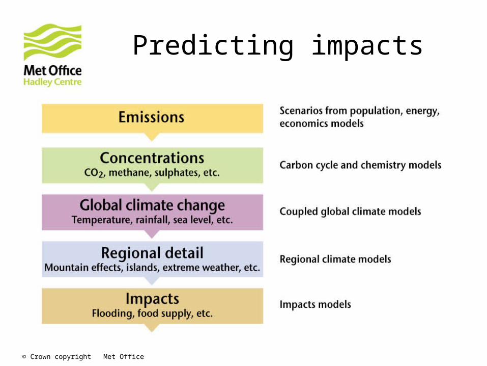
Predicting impacts

© Crown copyright Met Office
What is a Regional Climate Model? • Mathematical model of the atmosphere and land surface (and
sometimes the ocean)• ‘High’ resolution: Produces data in
grid cells < 50km in size• Spans a limited area (region) of the globe
• Contains representations of many of the important physical processes within the climate system
• Cloud• Radiation• Rainfall• Atmospheric aerosols• Soil hydrology• etc.
© Crown copyright Met Office
The components of PRECIS
• The RCM
• User interface to design and configure RCM experiments
• Display and data processing software
• Lateral boundary conditions (the input data)
• Training course and materials
• Technical and Scientific Support (by internet forum and email)
• Website (http://www.metoffice.gov.uk/precis)

© Crown copyright Met Office
The PRECIS user interface

© Crown copyright Met Office
• Region specification
• Choice of domain
• Land surface configuration
• RCM and Emissions scenario
• Period of the simulation
• Output data
• Run
PRECIS user interface: Main functionality
© Crown copyright Met Office
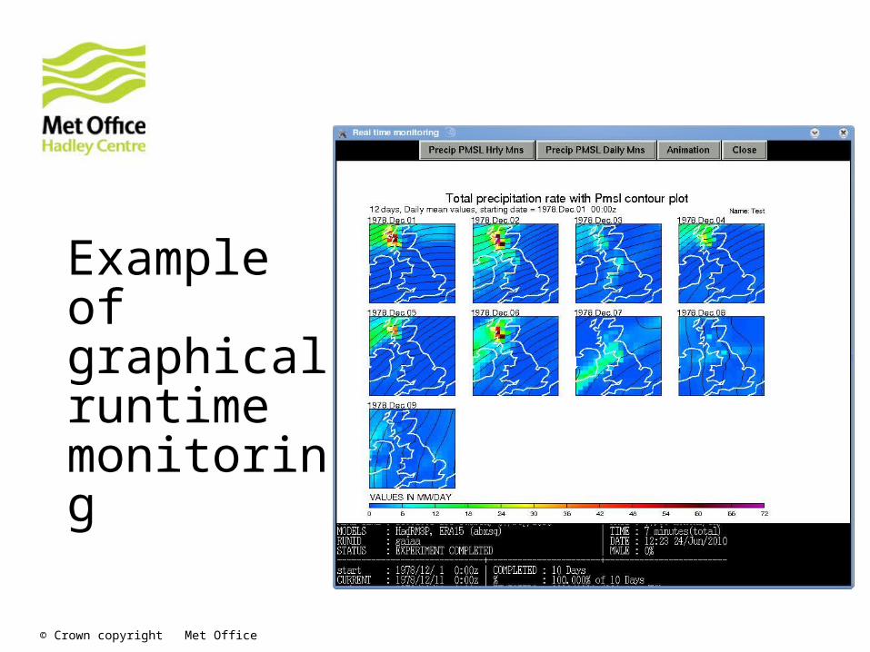
Example of graphical runtime monitoring
PRECIS user interface

© Crown copyright Met Office
How fast does it go?
• 1 core: ~ 2.5 months
• 4 cores:~ 2.75 weeks
• 8 cores:~ 12.5 days
30 year integration, 100x100, 50km grid points
Minimum hardware requirements
Computer: PC running under the Linux operating system
Memory : 512MB minimum; 1+ GB recommended
Minimum 250GB disk space + offline storage for archiving data
Simulation speed proportional to CPU speed

© Crown copyright Met Office
Support and follow-up
• Support• E-mail to the Hadley Centre ([email protected])
• Online discussion forum hosted by http://climateprediction.net
• Web site• http://www.metoffice.gov.uk/precis• news
• updates
• resources
• Collaboration/workshops

© Crown copyright Met Office
What PRECIS can deliver
• PRECIS can provide:
• climate scenarios for any region
• an estimate of uncertainty due to different emissions
• an estimate of uncertainty due to climate variability
• Data available from PRECIS
• Comprehensive and consistent meteorological and physical data for the atmosphere and land-surface
• Hourly and daily data as well as longer timescale averages
© Crown copyright Met Office
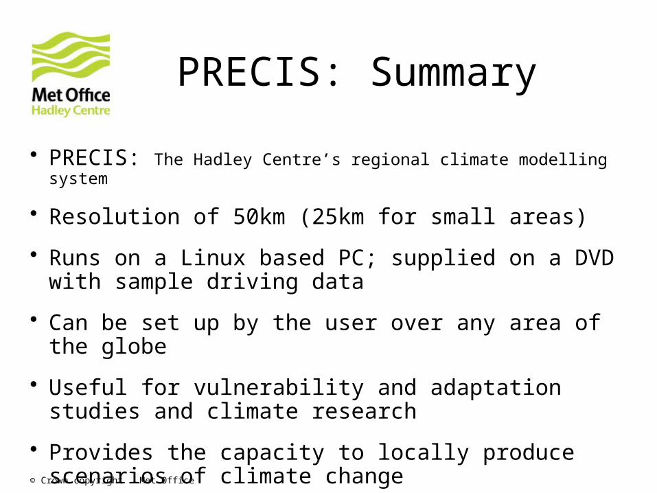
PRECIS: Summary
• PRECIS: The Hadley Centre’s regional climate modelling system
• Resolution of 50km (25km for small areas)
• Runs on a Linux based PC; supplied on a DVD with sample driving data
• Can be set up by the user over any area of the globe
• Useful for vulnerability and adaptation studies and climate research
• Provides the capacity to locally produce scenarios of climate change

© Crown copyright Met Office
Why downscaling?
© Crown copyright Met Office
Main reason: GCM lack regional details due to coarse resolution for many climate studies -> needs fine scale information to be derived from GCM output.
• Smaller scale climate results from an interaction between global climate and local physiographic details
• There is an increasing need to better understand the processes that determine regional climate
• Impact assessors need regional detail to assess vulnerability and possible adaptation strategies
Why downscaling?

… from a GCM grid to the point of interest.
From global to local climate …

© Crown copyright Met Office
How to downscale?

© Crown copyright Met Office
Downscaling techniques
• Statistical: based on statistical relationship between large- and local- scale
fine scale value = F (large-scale variables)
• Dynamical: Numerical models at high resolution over region of interest
• high resolution AGCM, limited area model (regional climate model)
• Statistical/Dynamical
Coarse atmospheric data (T, Q, winds, pressure etc)
Local atmospheric data (T, Q, winds, pressure etc)
100-300km
50km-1km: region, city,Fields etc

© Crown copyright Met Office
Statistical Downscaling

• Weather generators
• Markov chain, spell length
• Transfer functions
• linear regression, piecewise interpolation, artificial neural networks
• Weather typing
• Analogue methods, classification and tree analysis
Categories of statistical techniques

Relies on large-scale predictors for which Climate System Models are most skilful:
• Several grid lengths• Tropospheric variables (away from the surface)• Dynamic variables (geopotential, wind, temperature)
The transfer function must remain valid in different climate conditions:
• Hard to demonstrate• Can be evaluated by comparison with other approaches
The predictors must encompass the entire climate change signal:
• Importance of testing several predictors• Uncertainties related to the choice of predictors
Assumptions made for statistical downscaling

© Crown copyright Met Office
Regional climate models(Dynamical downscaling)

What is a Regional Climate Model?
• Comprehensive physical high resolution climate model that covers a limited area of the globe
• Includes the atmosphere and land surface components of the climate system (at least)
• Contains representations of the important processes within the climate system
• e.g. clouds, radiation, precipitation

© Crown copyright Met Office
One way nesting methodology
• A RCM is a limited area model (LAM), similar to those used in numerical weather prediction (NWP), i.e. short term weather forecasting
• LAMs are driven at the boundaries by GCM or observed data
• Lateral (side) and bottom (sea surface)
• LAMs are highly dependent on their boundary conditions and can not exist without them

© Crown copyright Met Office
Boundary conditions
Limited area regional models require meteorological information at their edges (lateral boundaries)
This data provides the interface between the regional model’s domain and the rest of the world.
The climate of a region is always strongly influenced by the global situation
These data are necessarily provided by global general circulation models (GCMs)
or from observed datasets with global coverage (re-analysis experiments)

© Crown copyright Met Office
Lateral boundary conditions (I)
• LBCs = Meteorological boundary conditions at the lateral (side) boundaries of the RCM domain
• They constrain the RCM throughout its simulation
• Provide the information the RCM needs from outside its domain
• Data come from a GCM or observations
• Lateral boundary condition variables• Wind
• Temperature
• Water
• Pressure
• Aerosols
LBC
variables
LBC variables
LBC variablesLB
C v
aria
bles

• Relaxation method (PRECIS)
• Large scale forcing merged with internal solution over a lateral buffer zone
• Spectral nesting
• Large scale forcing of low wave number components
• Important issues
• Spatial resolution of driving data
• Updating frequency of driving data
State variables
State variables
RCM
interior
Lateral boundary conditions (II)

© Crown copyright Met Office
Sea surface boundary conditions
• Two methods of supplying SST and sea ice:
• Using outputs from a coupled AOGCM
• Need good quality simulation of SST and sea ice in model
• Necessary for future simulations
• Using observed values
• Useful for the present-day simulation.
• For future climate need add changes in SST and ice from a coupled GCM to the observed values – complicated

Sources of errors in RCMs
• The RCM adds fine detail to the large-scale and shouldn’t deviate from it.
• Two sources of error:
• Large scale driving fields (external)
• Model physical formulation (internal).

Simulation length
• Minimum period
• 10 years to reasonably study the mean climate
• Preferably
• 30 years to study higher order statistics, climate variability, extremes, etc

© Crown copyright Met Office
Added value of RCMs

© Crown copyright Met Office
RCMs simulate current climate more realistically
Patterns of present-day winter precipitation over Great Britain

© Crown copyright Met Office
Represent smaller islands
Projected changes in summer surface air temperature between present day and the end of the 21st century.

© Crown copyright Met Office
Predict climate change with more detail
Projected changes in winter precipitation between now and 2080s.

© Crown copyright Met Office
Simulate and predict changes in extremes more realistically
Frequency of winter days over the Alps with different daily rainfall thresholds.

© Crown copyright Met Office
Simulate cyclones and hurricanes
A tropical cyclone is evident in the RCM (right) but not in the GCM

RCM data can be used to drive other models
A cyclone in the Bay of Bengal simulated by an RCM and the resulting high water levels in the Bay simulated by a coastal shelf model.

Crop impacts using high resolution projections from PRECIS
* Clear messages on future temperatures from the application of a regional climate model
* Precipitation projections are less certain, giving climate change information with different levels of confidence
* Application of this information to assess climate change impacts on crops still provides clear messages for the need for adaptation
© Crown copyright Met Office
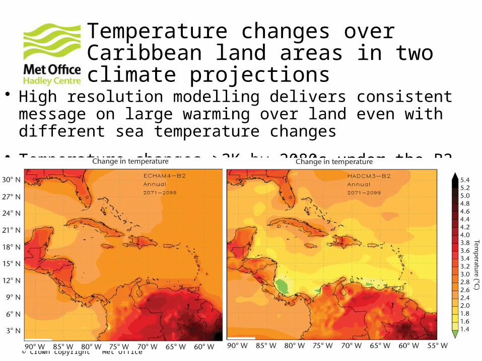
Temperature changes over Caribbean land areas in two climate projections
• High resolution modelling delivers consistent message on large warming over land even with different sea temperature changes
• Temperature changes >3K by 2080s under the B2 scenario
© Crown copyright Met Office
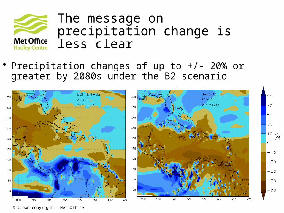
The message on precipitation change is less clear
• Precipitation changes of up to +/- 20% or greater by 2080s under the B2 scenario

© Crown copyright Met Office
Clear impact on Caribbean crops in 2050s with +2ºC and+/-20% precip.
Crop Temperature Change
(oC)
% Change in Precipitation
Yield (kg/ha)
Change in Yield
Rice
0
+2
+2
0
+20
-20
3356
3014
2888
-10%
-14%
Beans
0
+2
+2
0
+20
-20
1354
1164
1093
-14%
-19%
Maize
0
+2
+2
0
+20
-20
4511
3737
3759
-22%
-17%
Crop Temperature Change
(oC)
% Change in Precipitation
Yield (kg/ha)
Change in Yield
Rice
0
+2
+2
0
+20
-20
3356
3014
2888
-10%
-14%
Beans
0
+2
+2
0
+20
-20
1354
1164
1093
-14%
-19%
Maize
0
+2
+2
0
+20
-20
4511
3737
3759
-22%
-17%
Table: Simulated crop yields under current climate and with a 2 ºC temperature increase accompanied by either a 20% increase or decrease in rainfall.

Suitability of regionalisation techniques
Method Strengths Weaknesses
Statistical · High resolution· Computation
ally cheap
· Dependent on empiricalrelationships derived for present-day climate
· Few variables available· Not easily relocatable
High-resAGCMs
· Dependent on surface boundaryconditions from couple model
· Computationally expensive
Regionalmodels
· High (very high)resolution
· Can representextremes
· Physically based· Many variables· RCM: easily
relocatable
· Dependent on driving model &surface boundary conditions· Possible lack of two-way nesting· Computationally expensive· (Have to parameterise across
scales )

© Crown copyright Met Office
Summary
• Downscaling techniques are used to add fine scale details to a GCM projection
• Several methods are available with their own strengths and weaknesses
• PRECIS is a physically-based and computationally accessible regional climate model for downscaling GCM projections

© Crown copyright Met Office
Questions


