Computing and
decomposing tensors
— Decomposition basics
Nick Vannieuwenhoven(FWO / KU Leuven)
Computing and decomposing tensors: Decomposition basics
1 Introduction
2 Basic tensor operations
3 Tucker decompositionMultilinear rankHigher-order singular value decompositionNumerical issuesTruncation algorithms
4 Tensor rank decompositionRankBorder rankIdentifiability
5 References
Computing and decomposing tensors: Decomposition basics
Introduction
Overview
1 Introduction
2 Basic tensor operations
3 Tucker decompositionMultilinear rankHigher-order singular value decompositionNumerical issuesTruncation algorithms
4 Tensor rank decompositionRankBorder rankIdentifiability
5 References
Computing and decomposing tensors: Decomposition basics
Introduction
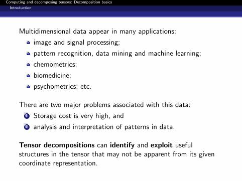
Multidimensional data appear in many applications:
image and signal processing;
pattern recognition, data mining and machine learning;
chemometrics;
biomedicine;
psychometrics; etc.
There are two major problems associated with this data:
1 Storage cost is very high, and
2 analysis and interpretation of patterns in data.
Tensor decompositions can identify and exploit usefulstructures in the tensor that may not be apparent from its givencoordinate representation.
Computing and decomposing tensors: Decomposition basics
Introduction
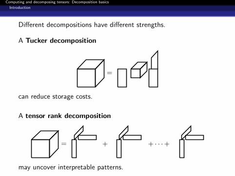
Different decompositions have different strengths.
A Tucker decomposition
=
can reduce storage costs.
A tensor rank decomposition
= + + · · ·+
may uncover interpretable patterns.
Computing and decomposing tensors: Decomposition basics
Basic tensor operations
Overview
1 Introduction
2 Basic tensor operations
3 Tucker decompositionMultilinear rankHigher-order singular value decompositionNumerical issuesTruncation algorithms
4 Tensor rank decompositionRankBorder rankIdentifiability
5 References
Computing and decomposing tensors: Decomposition basics
Basic tensor operations
Flattenings
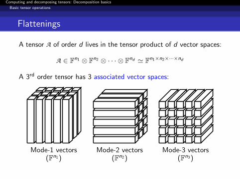
A tensor A of order d lives in the tensor product of d vector spaces:
A ∈ Fn1 ⊗ Fn2 ⊗ · · · ⊗ Fnd ' Fn1×n2×···×nd
A 3rd order tensor has 3 associated vector spaces:
Mode-1 vectors(Fn1)
Mode-2 vectors(Fn2)
Mode-3 vectors(Fn3)
Computing and decomposing tensors: Decomposition basics
Basic tensor operations
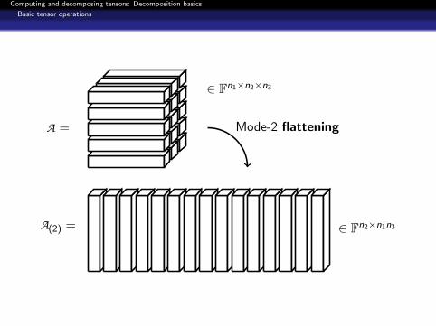
A =
A(2) =
∈ Fn1×n2×n3
∈ Fn2×n1n3
Mode-2 flattening
Computing and decomposing tensors: Decomposition basics
Basic tensor operations
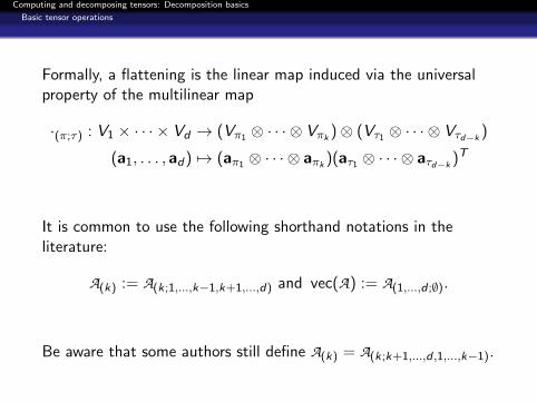
Formally, a flattening is the linear map induced via the universalproperty of the multilinear map
·(π;τ) : V1 × · · · × Vd → (Vπ1 ⊗ · · · ⊗ Vπk )⊗ (Vτ1 ⊗ · · · ⊗ Vτd−k)
(a1, . . . , ad) 7→ (aπ1 ⊗ · · · ⊗ aπk )(aτ1 ⊗ · · · ⊗ aτd−k)T
It is common to use the following shorthand notations in theliterature:
A(k) := A(k;1,...,k−1,k+1,...,d) and vec(A) := A(1,...,d ;∅).
Be aware that some authors still define A(k) = A(k;k+1,...,d ,1,...,k−1).
Computing and decomposing tensors: Decomposition basics
Basic tensor operations
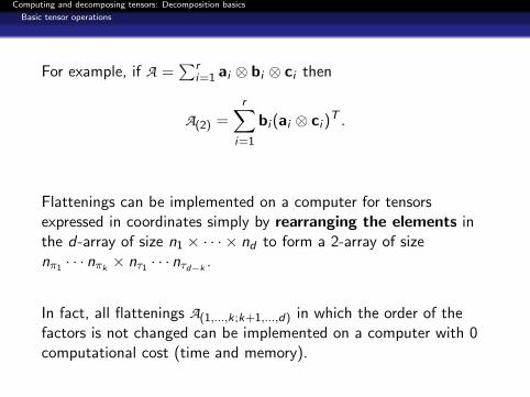
For example, if A =∑r
i=1 ai ⊗ bi ⊗ ci then
A(2) =r∑
i=1
bi (ai ⊗ ci )T .
Flattenings can be implemented on a computer for tensorsexpressed in coordinates simply by rearranging the elements inthe d-array of size n1 × · · · × nd to form a 2-array of sizenπ1 · · · nπk × nτ1 · · · nτd−k
.
In fact, all flattenings A(1,...,k;k+1,...,d) in which the order of thefactors is not changed can be implemented on a computer with 0computational cost (time and memory).
Computing and decomposing tensors: Decomposition basics
Basic tensor operations
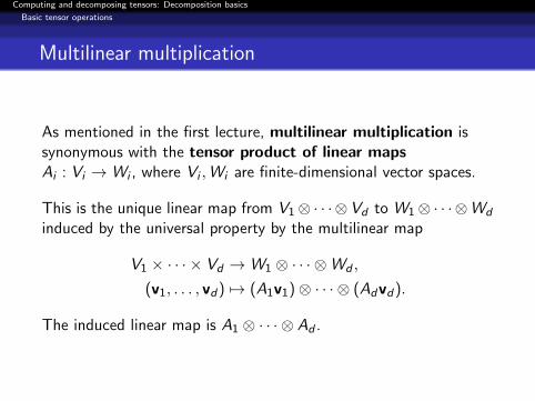
Multilinear multiplication
As mentioned in the first lecture, multilinear multiplication issynonymous with the tensor product of linear mapsAi : Vi →Wi , where Vi ,Wi are finite-dimensional vector spaces.
This is the unique linear map from V1⊗ · · · ⊗Vd to W1⊗ · · · ⊗Wd
induced by the universal property by the multilinear map
V1 × · · · × Vd →W1 ⊗ · · · ⊗Wd ,
(v1, . . . , vd) 7→ (A1v1)⊗ · · · ⊗ (Advd).
The induced linear map is A1 ⊗ · · · ⊗ Ad .
Computing and decomposing tensors: Decomposition basics
Basic tensor operations
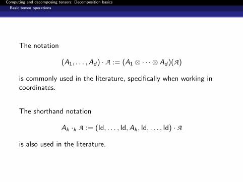
The notation
(A1, . . . ,Ad) · A := (A1 ⊗ · · · ⊗ Ad)(A)
is commonly used in the literature, specifically when working incoordinates.
The shorthand notation
Ak ·k A := (Id, . . . , Id,Ak , Id, . . . , Id) · A
is also used in the literature.
Computing and decomposing tensors: Decomposition basics
Basic tensor operations
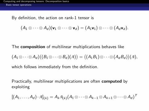
By definition, the action on rank-1 tensor is
(A1 ⊗ · · · ⊗ Ad)(v1 ⊗ · · · ⊗ vd) = (A1v1)⊗ · · · ⊗ (Advd).
The composition of multilinear multiplications behaves like
(A1⊗· · ·⊗Ad)((B1⊗· · ·⊗Bd)(A)
)=((A1B1)⊗· · ·⊗(AdBd)
)(A),
which follows immediately from the definition.
Practically, multilinear multiplications are often computed byexploiting
[(A1, . . . ,Ad) ·A](k) = AkA(k)(A1⊗· · ·⊗Ak−1⊗Ak+1⊗· · ·⊗Ad)T
Computing and decomposing tensors: Decomposition basics
Tucker decomposition
Overview
1 Introduction
2 Basic tensor operations
3 Tucker decompositionMultilinear rankHigher-order singular value decompositionNumerical issuesTruncation algorithms
4 Tensor rank decompositionRankBorder rankIdentifiability
5 References
Computing and decomposing tensors: Decomposition basics
Tucker decomposition
Multilinear rank
Multilinear rank
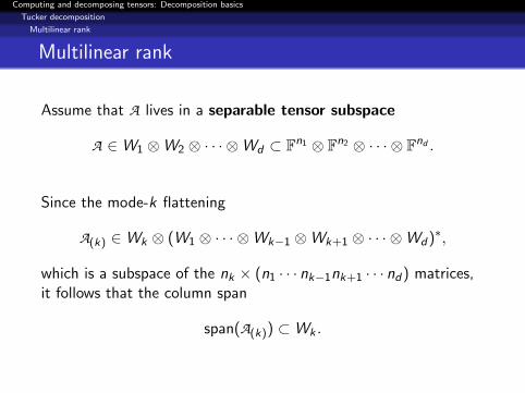
Assume that A lives in a separable tensor subspace
A ∈W1 ⊗W2 ⊗ · · · ⊗Wd ⊂ Fn1 ⊗ Fn2 ⊗ · · · ⊗ Fnd .
Since the mode-k flattening
A(k) ∈Wk ⊗ (W1 ⊗ · · · ⊗Wk−1 ⊗Wk+1 ⊗ · · · ⊗Wd)∗,
which is a subspace of the nk × (n1 · · · nk−1nk+1 · · · nd) matrices,it follows that the column span
span(A(k)) ⊂Wk .
Computing and decomposing tensors: Decomposition basics
Tucker decomposition
Multilinear rank
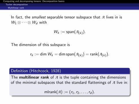
In fact, the smallest separable tensor subspace that A lives in isW1 ⊗ · · · ⊗Wd with
Wk := span(A(k)).
The dimension of this subspace is
rk := dim Wk = dim span(A(k)) = rank(A(k)).
Definition (Hitchcock, 1928)
The multilinear rank of A is the tuple containing the dimensionsof the minimal subspaces that the standard flattenings of A live in:
mlrank(A) := (r1, r2, . . . , rd).
Computing and decomposing tensors: Decomposition basics
Tucker decomposition
Multilinear rank
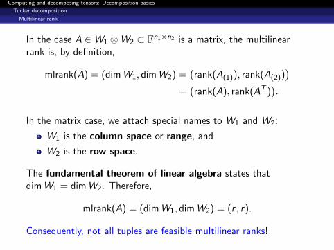
In the case A ∈W1 ⊗W2 ⊂ Fn1×n2 is a matrix, the multilinearrank is, by definition,
mlrank(A) = (dim W1, dim W2) =(rank(A(1)), rank(A(2))
)=(rank(A), rank(AT )
).
In the matrix case, we attach special names to W1 and W2:
W1 is the column space or range, and
W2 is the row space.
The fundamental theorem of linear algebra states thatdim W1 = dim W2. Therefore,
mlrank(A) = (dim W1, dim W2) = (r , r).
Consequently, not all tuples are feasible multilinear ranks!
Computing and decomposing tensors: Decomposition basics
Tucker decomposition
Multilinear rank
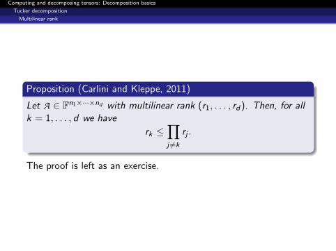
Proposition (Carlini and Kleppe, 2011)
Let A ∈ Fn1×···×nd with multilinear rank (r1, . . . , rd). Then, for allk = 1, . . . , d we have
rk ≤∏j 6=k
rj .
The proof is left as an exercise.
Computing and decomposing tensors: Decomposition basics
Tucker decomposition
Multilinear rank
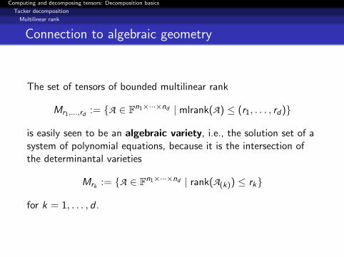
Connection to algebraic geometry
The set of tensors of bounded multilinear rank
Mr1,...,rd := {A ∈ Fn1×···×nd | mlrank(A) ≤ (r1, . . . , rd)}
is easily seen to be an algebraic variety, i.e., the solution set of asystem of polynomial equations, because it is the intersection ofthe determinantal varieties
Mrk := {A ∈ Fn1×···×nd | rank(A(k)) ≤ rk}
for k = 1, . . . , d .
Computing and decomposing tensors: Decomposition basics
Tucker decomposition
Higher-order singular value decomposition
Overview
1 Introduction
2 Basic tensor operations
3 Tucker decompositionMultilinear rankHigher-order singular value decompositionNumerical issuesTruncation algorithms
4 Tensor rank decompositionRankBorder rankIdentifiability
5 References
Computing and decomposing tensors: Decomposition basics
Tucker decomposition
Higher-order singular value decomposition
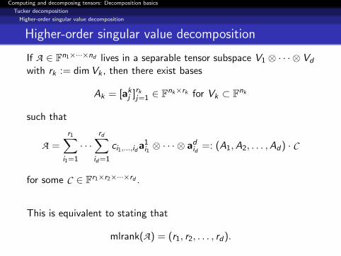
Higher-order singular value decomposition
If A ∈ Fn1×···×nd lives in a separable tensor subspace V1 ⊗ · · · ⊗ Vd
with rk := dim Vk , then there exist bases
Ak = [akj ]rkj=1 ∈ Fnk×rk for Vk ⊂ Fnk
such that
A =
r1∑i1=1
· · ·rd∑
id=1
ci1,...,id a1i1 ⊗ · · · ⊗ ad
id=: (A1,A2, . . . ,Ad) · C
for some C ∈ Fr1×r2×···×rd .
This is equivalent to stating that
mlrank(A) = (r1, r2, . . . , rd).
Computing and decomposing tensors: Decomposition basics
Tucker decomposition
Higher-order singular value decomposition
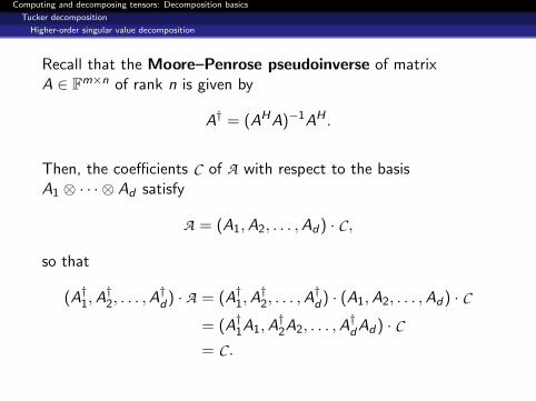
Recall that the Moore–Penrose pseudoinverse of matrixA ∈ Fm×n of rank n is given by
A† = (AHA)−1AH .
Then, the coefficients C of A with respect to the basisA1 ⊗ · · · ⊗ Ad satisfy
A = (A1,A2, . . . ,Ad) · C ,
so that
(A†1,A†2, . . . ,A
†d) · A = (A†1,A
†2, . . . ,A
†d) · (A1,A2, . . . ,Ad) · C
= (A†1A1,A†2A2, . . . ,A
†dAd) · C
= C .
Computing and decomposing tensors: Decomposition basics
Tucker decomposition
Higher-order singular value decomposition
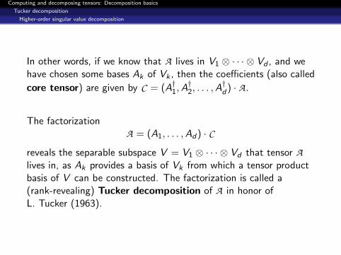
In other words, if we know that A lives in V1 ⊗ · · · ⊗ Vd , and wehave chosen some bases Ak of Vk , then the coefficients (also called
core tensor) are given by C = (A†1,A†2, . . . ,A
†d) · A.
The factorizationA = (A1, . . . ,Ad) · C
reveals the separable subspace V = V1 ⊗ · · · ⊗ Vd that tensor Alives in, as Ak provides a basis of Vk from which a tensor productbasis of V can be constructed. The factorization is called a(rank-revealing) Tucker decomposition of A in honor ofL. Tucker (1963).
Computing and decomposing tensors: Decomposition basics
Tucker decomposition
Higher-order singular value decomposition
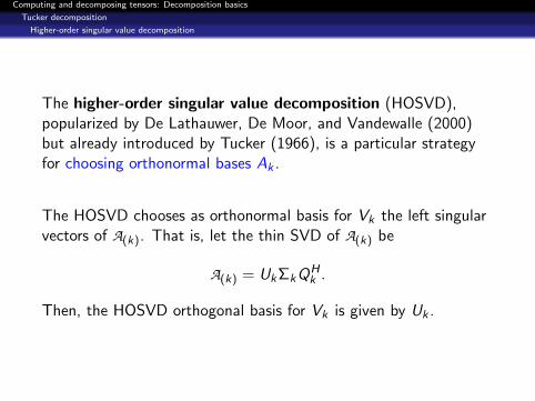
The higher-order singular value decomposition (HOSVD),popularized by De Lathauwer, De Moor, and Vandewalle (2000)but already introduced by Tucker (1966), is a particular strategyfor choosing orthonormal bases Ak .
The HOSVD chooses as orthonormal basis for Vk the left singularvectors of A(k). That is, let the thin SVD of A(k) be
A(k) = UkΣkQHk .
Then, the HOSVD orthogonal basis for Vk is given by Uk .

Computing and decomposing tensors: Decomposition basics
Tucker decomposition
Higher-order singular value decomposition
An advantage of choosing orthonormal bases Ak , beyond improvednumerical stability, is that the Moore–Penrose inverse reduces to
U†k = (UHk Uk)−1UH
k = UHk ,
so that
A = (U1,U2, . . . ,Ud) ·((U1,U2, . . . ,Ud)H · A
)= (U1UH
1 ,U2UH2 , . . . ,UdUH
d ) · A= π1π2 · · ·πdA
whereπkA := (UkUH
k ) ·k A
is the HOSVD mode-k orthogonal projection.
Computing and decomposing tensors: Decomposition basics
Tucker decomposition
Higher-order singular value decomposition
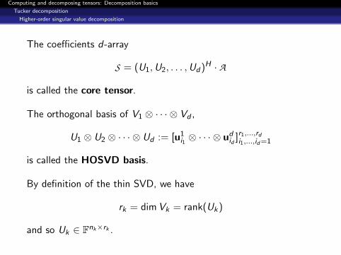
The coefficients d-array
S = (U1,U2, . . . ,Ud)H · A
is called the core tensor.
The orthogonal basis of V1 ⊗ · · · ⊗ Vd ,
U1 ⊗ U2 ⊗ · · · ⊗ Ud := [u1i1 ⊗ · · · ⊗ ud
id]r1,...,rdi1,...,id=1
is called the HOSVD basis.
By definition of the thin SVD, we have
rk = dim Vk = rank(Uk)
and so Uk ∈ Fnk×rk .
Computing and decomposing tensors: Decomposition basics
Tucker decomposition
Higher-order singular value decomposition
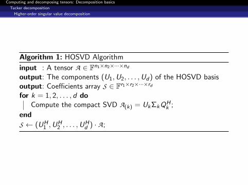
Algorithm 1: HOSVD Algorithm
input : A tensor A ∈ Fn1×n2×···×nd
output: The components (U1,U2, . . . ,Ud) of the HOSVD basisoutput: Coefficients array S ∈ Fr1×r2×···×rd
for k = 1, 2, . . . , d doCompute the compact SVD A(k) = UkΣkQH
k ;
end
S ← (UH1 ,U
H2 , . . . ,U
Hd ) · A;
Computing and decomposing tensors: Decomposition basics
Tucker decomposition
Higher-order singular value decomposition
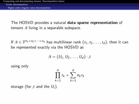
The HOSVD provides a natural data sparse representation oftensors A living in a separable subspace.
If A ∈ Fn1×n2×···×nd has multilinear rank (r1, r2, . . . , rd), then it canbe represented exactly via the HOSVD as
A = (U1,U2, . . . ,Ud) · S
using onlyd∏
k=1
rk +d∑
k=1
nk rk
storage (for S and the Ui ).
Computing and decomposing tensors: Decomposition basics
Tucker decomposition
Numerical issues
Overview
1 Introduction
2 Basic tensor operations
3 Tucker decompositionMultilinear rankHigher-order singular value decompositionNumerical issuesTruncation algorithms
4 Tensor rank decompositionRankBorder rankIdentifiability
5 References
Computing and decomposing tensors: Decomposition basics
Tucker decomposition
Numerical issues
Numerical issues
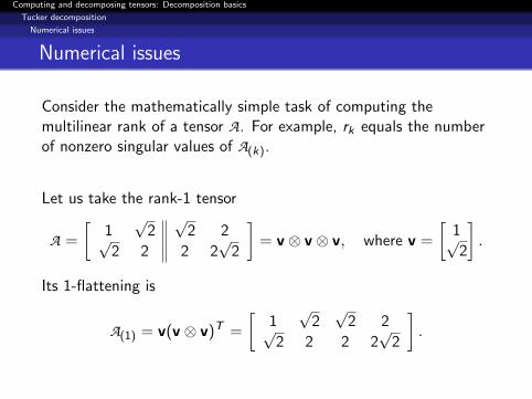
Consider the mathematically simple task of computing themultilinear rank of a tensor A. For example, rk equals the numberof nonzero singular values of A(k).
Let us take the rank-1 tensor
A =
[1√
2√
2 2√2 2 2 2
√2
]= v ⊗ v ⊗ v, where v =
[1√2
].
Its 1-flattening is
A(1) = v(v ⊗ v)T =
[1√
2√
2 2√2 2 2 2
√2
].
Computing and decomposing tensors: Decomposition basics
Tucker decomposition
Numerical issues
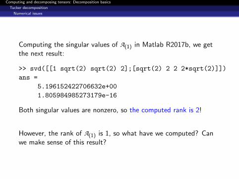
Computing the singular values of A(1) in Matlab R2017b, we getthe next result:
>> svd([[1 sqrt(2) sqrt(2) 2];[sqrt(2) 2 2 2*sqrt(2)]])
ans =
5.196152422706632e+00
1.805984985273179e-16
Both singular values are nonzero, so the computed rank is 2!
However, the rank of A(1) is 1, so what have we computed? Canwe make sense of this result?
Computing and decomposing tensors: Decomposition basics
Tucker decomposition
Numerical issues
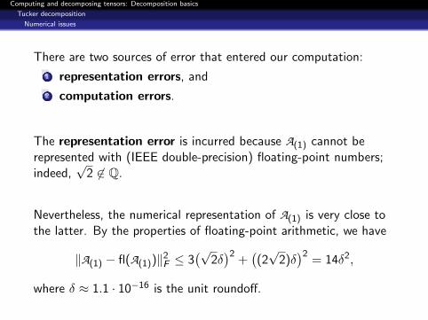
There are two sources of error that entered our computation:
1 representation errors, and
2 computation errors.
The representation error is incurred because A(1) cannot berepresented with (IEEE double-precision) floating-point numbers;indeed,
√2 6∈ Q.
Nevertheless, the numerical representation of A(1) is very close tothe latter. By the properties of floating-point arithmetic, we have
‖A(1) − fl(A(1))‖2F ≤ 3
(√2δ)2
+((2√
2)δ)2
= 14δ2,
where δ ≈ 1.1 · 10−16 is the unit roundoff.
Computing and decomposing tensors: Decomposition basics
Tucker decomposition
Numerical issues
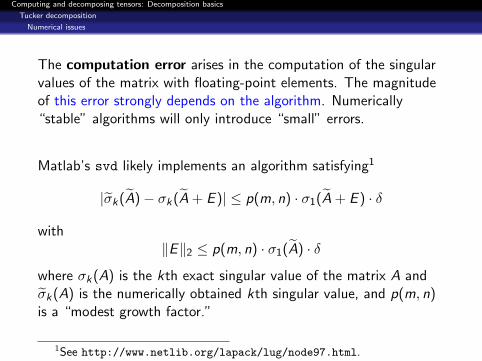
The computation error arises in the computation of the singularvalues of the matrix with floating-point elements. The magnitudeof this error strongly depends on the algorithm. Numerically“stable” algorithms will only introduce “small” errors.
Matlab’s svd likely implements an algorithm satisfying1
|σk(A)− σk(A + E )| ≤ p(m, n) · σ1(A + E ) · δ
with‖E‖2 ≤ p(m, n) · σ1(A) · δ
where σk(A) is the kth exact singular value of the matrix A andσk(A) is the numerically obtained kth singular value, and p(m, n)is a “modest growth factor.”
1See http://www.netlib.org/lapack/lug/node97.html.
Computing and decomposing tensors: Decomposition basics
Tucker decomposition
Numerical issues
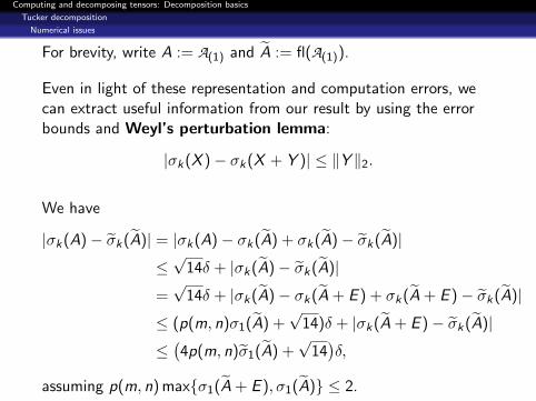
For brevity, write A := A(1) and A := fl(A(1)).
Even in light of these representation and computation errors, wecan extract useful information from our result by using the errorbounds and Weyl’s perturbation lemma:
|σk(X )− σk(X + Y )| ≤ ‖Y ‖2.
We have
|σk(A)− σk(A)| = |σk(A)− σk(A) + σk(A)− σk(A)|
≤√
14δ + |σk(A)− σk(A)|
=√
14δ + |σk(A)− σk(A + E ) + σk(A + E )− σk(A)|
≤ (p(m, n)σ1(A) +√
14)δ + |σk(A + E )− σk(A)|
≤(4p(m, n)σ1(A) +
√14)δ,
assuming p(m, n) max{σ1(A + E ), σ1(A)} ≤ 2.
Computing and decomposing tensors: Decomposition basics
Tucker decomposition
Numerical issues
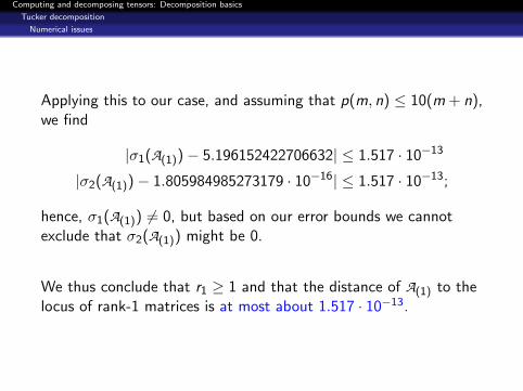
Applying this to our case, and assuming that p(m, n) ≤ 10(m + n),we find
|σ1(A(1))− 5.196152422706632| ≤ 1.517 · 10−13
|σ2(A(1))− 1.805984985273179 · 10−16| ≤ 1.517 · 10−13;
hence, σ1(A(1)) 6= 0, but based on our error bounds we cannotexclude that σ2(A(1)) might be 0.
We thus conclude that r1 ≥ 1 and that the distance of A(1) to thelocus of rank-1 matrices is at most about 1.517 · 10−13.
Computing and decomposing tensors: Decomposition basics
Tucker decomposition
Truncation algorithms
Overview
1 Introduction
2 Basic tensor operations
3 Tucker decompositionMultilinear rankHigher-order singular value decompositionNumerical issuesTruncation algorithms
4 Tensor rank decompositionRankBorder rankIdentifiability
5 References
Computing and decomposing tensors: Decomposition basics
Tucker decomposition
Truncation algorithms
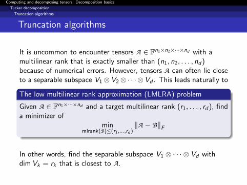
Truncation algorithms
It is uncommon to encounter tensors A ∈ Fn1×n2×···×nd with amultilinear rank that is exactly smaller than (n1, n2, . . . , nd)because of numerical errors. However, tensors A can often lie closeto a separable subspace V1⊗V2⊗ · · · ⊗Vd . This leads naturally to
The low multilinear rank approximation (LMLRA) problem
Given A ∈ Fn1×···×nd and a target multilinear rank (r1, . . . , rd), finda minimizer of
minmlrank(B)≤(r1,...,rd )
‖A − B‖F
In other words, find the separable subspace V1 ⊗ · · · ⊗ Vd withdim Vk = rk that is closest to A.
Computing and decomposing tensors: Decomposition basics
Tucker decomposition
Truncation algorithms
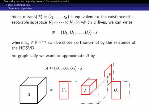
Since mlrank(B) = (r1, . . . , rd) is equivalent to the existence of aseparable subspace V1 ⊗ · · · ⊗ Vd in which B lives, we can write
B = (U1,U2, . . . ,Ud) · S
where Uk ∈ Fnk×rk can be chosen orthonormal by the existence ofthe HOSVD.
So graphically we want to approximate A by
A ≈ (U1,U2,U3) · S
A≈ U1 U2
U3
S
Computing and decomposing tensors: Decomposition basics
Tucker decomposition
Truncation algorithms
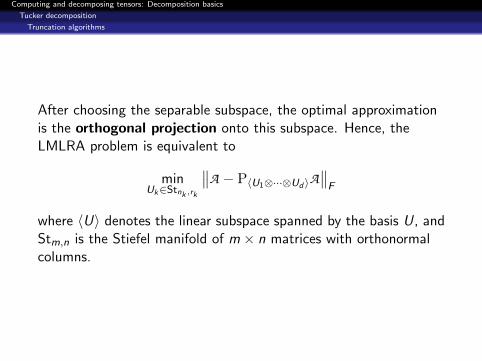
After choosing the separable subspace, the optimal approximationis the orthogonal projection onto this subspace. Hence, theLMLRA problem is equivalent to
minUk∈Stnk ,rk
∥∥A − P〈U1⊗···⊗Ud 〉A∥∥F
where 〈U〉 denotes the linear subspace spanned by the basis U, andStm,n is the Stiefel manifold of m × n matrices with orthonormalcolumns.
Computing and decomposing tensors: Decomposition basics
Tucker decomposition
Truncation algorithms
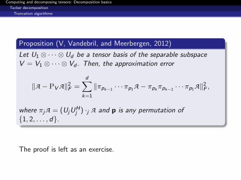
Proposition (V, Vandebril, and Meerbergen, 2012)
Let U1 ⊗ · · · ⊗ Ud be a tensor basis of the separable subspaceV = V1 ⊗ · · · ⊗ Vd . Then, the approximation error
‖A − PV A‖2F =
d∑k=1
‖πpk−1· · ·πp1 A − πpkπpk−1
· · ·πp1 A‖2F ,
where πjA = (UjUHj ) ·j A and p is any permutation of
{1, 2, . . . , d}.
The proof is left as an exercise.
Computing and decomposing tensors: Decomposition basics
Tucker decomposition
Truncation algorithms
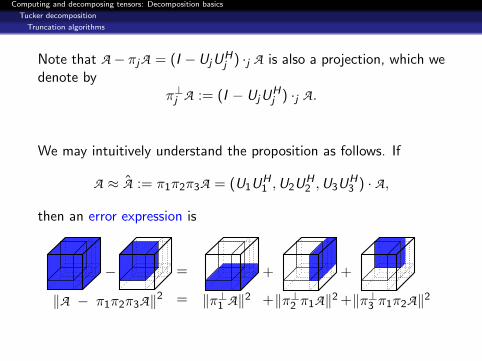
Note that A − πjA = (I −UjUHj ) ·j A is also a projection, which we
denote byπ⊥j A := (I − UjU
Hj ) ·j A.
We may intuitively understand the proposition as follows. If
A ≈ A := π1π2π3A = (U1UH1 ,U2UH
2 ,U3UH3 ) · A,
then an error expression is
− =
=‖A − π1π2π3A‖2
+ +
+ +‖π⊥1 A‖2 ‖π⊥2 π1A‖2 ‖π⊥3 π1π2A‖2
Computing and decomposing tensors: Decomposition basics
Tucker decomposition
Truncation algorithms
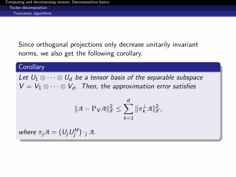
Since orthogonal projections only decrease unitarily invariantnorms, we also get the following corollary.
Corollary
Let U1 ⊗ · · · ⊗ Ud be a tensor basis of the separable subspaceV = V1 ⊗ · · · ⊗ Vd . Then, the approximation error satisfies
‖A − PV A‖2F ≤
d∑k=1
‖π⊥k A‖2F ,
where πjA = (UjUHj ) ·j A.
Computing and decomposing tensors: Decomposition basics
Tucker decomposition
Truncation algorithms
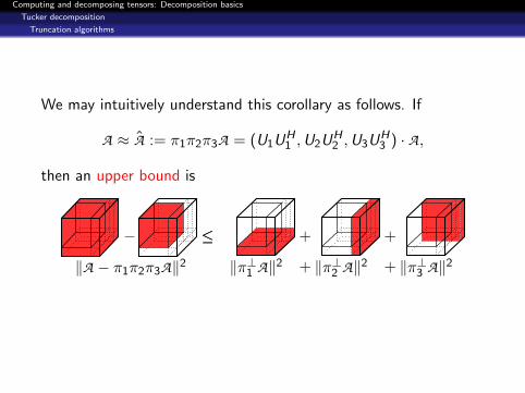
We may intuitively understand this corollary as follows. If
A ≈ A := π1π2π3A = (U1UH1 ,U2UH
2 ,U3UH3 ) · A,
then an upper bound is
− ≤≤
‖A − π1π2π3A‖2
+ +
+ +‖π⊥1 A‖2 ‖π⊥2 A‖2 ‖π⊥3 A‖2
Computing and decomposing tensors: Decomposition basics
Tucker decomposition
Truncation algorithms
A closed solution of the LMLRA problem
minUk∈Stnk ,rk
∥∥A − P〈U1⊗···⊗Ud 〉A∥∥F
is not known.
However, we can use foregoing error expressions for choosing good,even quasi-optimal, separable subspaces to project onto.
Computing and decomposing tensors: Decomposition basics
Tucker decomposition
Truncation algorithms
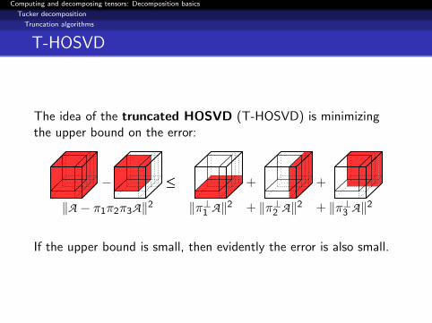
T-HOSVD
The idea of the truncated HOSVD (T-HOSVD) is minimizingthe upper bound on the error:
− ≤≤
‖A − π1π2π3A‖2
+ +
+ +‖π⊥1 A‖2 ‖π⊥2 A‖2 ‖π⊥3 A‖2
If the upper bound is small, then evidently the error is also small.
Computing and decomposing tensors: Decomposition basics
Tucker decomposition
Truncation algorithms
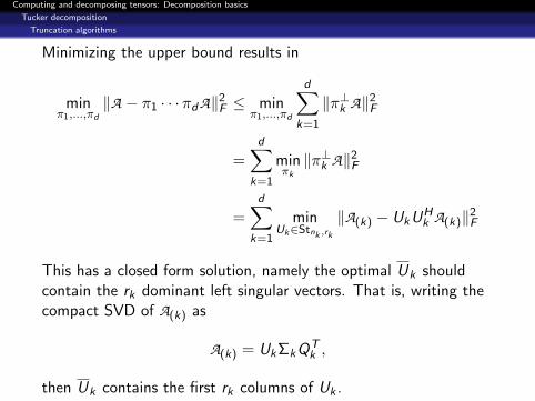
Minimizing the upper bound results in
minπ1,...,πd
‖A − π1 · · ·πdA‖2F ≤ min
π1,...,πd
d∑k=1
‖π⊥k A‖2F
=d∑
k=1
minπk‖π⊥k A‖2
F
=d∑
k=1
minUk∈Stnk ,rk
‖A(k) − UkUHk A(k)‖2
F
This has a closed form solution, namely the optimal Uk shouldcontain the rk dominant left singular vectors. That is, writing thecompact SVD of A(k) as
A(k) = UkΣkQTk ,
then Uk contains the first rk columns of Uk .
Computing and decomposing tensors: Decomposition basics
Tucker decomposition
Truncation algorithms
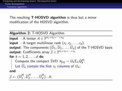
The resulting T-HOSVD algorithm is thus but a minormodification of the HOSVD algorithm.
Algorithm 2: T-HOSVD Algorithm
input : A tensor A ∈ Fn1×n2×···×nd
input : A target multilinear rank (r1, r2, . . . , rd).output: The components (U1,U2, . . . ,Ud) of the T-HOSVD basisoutput: Coefficients array S ∈ Fr1×r2×···×rd
for k = 1, 2, . . . , d doCompute the compact SVD A(k) = UkΣkQH
k ;
Let Uk contain the first rk columns of Uk ;
end
S ← (UH1 ,U
H2 , . . . ,U
Hd ) · A;
Computing and decomposing tensors: Decomposition basics
Tucker decomposition
Truncation algorithms
Assume that we truncate a tensor in Fn×···×n to multilinear rank(r , . . . , r). The computational complexity of standard T-HOSVD is
O
(dnd+1 +
d∑k=1
nd+1−k rk
)operations.
Computing and decomposing tensors: Decomposition basics
Tucker decomposition
Truncation algorithms
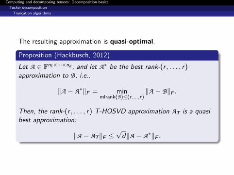
The resulting approximation is quasi-optimal.
Proposition (Hackbusch, 2012)
Let A ∈ Fn1×···×nd , and let A∗ be the best rank-(r , . . . , r)approximation to B, i.e.,
‖A − A∗‖F = minmlrank(B)≤(r ,...,r)
‖A − B‖F .
Then, the rank-(r , . . . , r) T-HOSVD approximation AT is a quasibest approximation:
‖A − AT‖F ≤√
d‖A − A∗‖F .
Computing and decomposing tensors: Decomposition basics
Tucker decomposition
Truncation algorithms
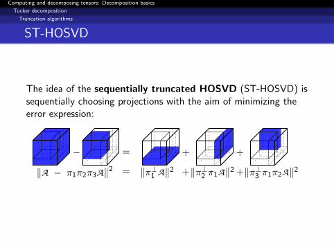
ST-HOSVD
The idea of the sequentially truncated HOSVD (ST-HOSVD) issequentially choosing projections with the aim of minimizing theerror expression:
− =
=‖A − π1π2π3A‖2
+ +
+ +‖π⊥1 A‖2 ‖π⊥2 π1A‖2 ‖π⊥3 π1π2A‖2
Computing and decomposing tensors: Decomposition basics
Tucker decomposition
Truncation algorithms
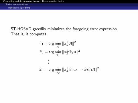
ST-HOSVD greedily minimizes the foregoing error expression.That is, it computes
π1 = arg minπ1
‖π⊥1 A‖2
π2 = arg minπ2
‖π⊥2 π1A‖2
...
πd = arg minπd‖π⊥d πd−1 · · · π2π1A‖2
Computing and decomposing tensors: Decomposition basics
Tucker decomposition
Truncation algorithms
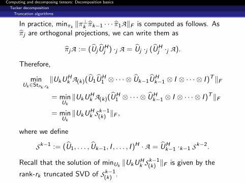
In practice, minπk ‖π⊥k πk−1 · · · π1A‖F is computed as follows. Asπj are orthogonal projections, we can write them as
πjA := (Uj UHj ) ·j A = Uj ·j (UH
j ·j A).
Therefore,
minUk∈Stnk ,rk
‖UkUHk A(k)(U1UH
1 ⊗ · · · ⊗ Uk−1UHk−1 ⊗ I ⊗ · · · ⊗ I )T‖F
= minUk
‖UkUHk A(k)(UH
1 ⊗ · · · ⊗ UHk−1 ⊗ I ⊗ · · · ⊗ I )T‖F
= minUk
‖UkUHk Sk−1
(k) ‖F ,
where we define
Sk−1 := (U1, . . . , Uk−1, I , . . . , I )H · A = UHk−1 ·k−1 Sk−2.
Recall that the solution of minUk‖UkUH
k Sk−1(k) ‖F is given by the
rank-rk truncated SVD of Sk−1(k) .
Computing and decomposing tensors: Decomposition basics
Tucker decomposition
Truncation algorithms
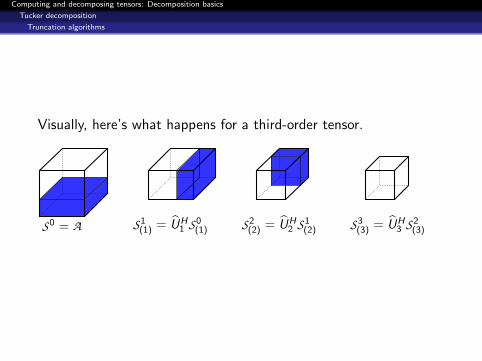
Visually, here’s what happens for a third-order tensor.
S0 = A S1(1) = UH
1 S0(1) S2
(2) = UH2 S1
(2) S3(3) = UH
3 S2(3)
Computing and decomposing tensors: Decomposition basics
Tucker decomposition
Truncation algorithms
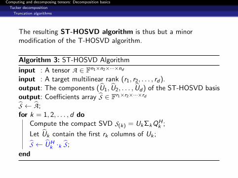
The resulting ST-HOSVD algorithm is thus but a minormodification of the T-HOSVD algorithm.
Algorithm 3: ST-HOSVD Algorithm
input : A tensor A ∈ Fn1×n2×···×nd
input : A target multilinear rank (r1, r2, . . . , rd).output: The components (U1, U2, . . . , Ud) of the ST-HOSVD basisoutput: Coefficients array S ∈ Fr1×r2×···×rd
S ← A;for k = 1, 2, . . . , d do
Compute the compact SVD S(k) = UkΣkQHk ;
Let Uk contain the first rk columns of Uk ;
S ← UHk ·k S ;
end
Computing and decomposing tensors: Decomposition basics
Tucker decomposition
Truncation algorithms
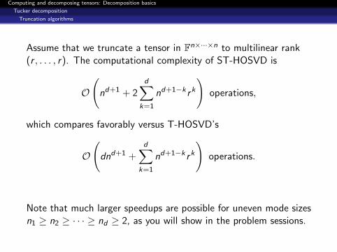
Assume that we truncate a tensor in Fn×···×n to multilinear rank(r , . . . , r). The computational complexity of ST-HOSVD is
O
(nd+1 + 2
d∑k=1
nd+1−k rk
)operations,
which compares favorably versus T-HOSVD’s
O
(dnd+1 +
d∑k=1
nd+1−k rk
)operations.
Note that much larger speedups are possible for uneven mode sizesn1 ≥ n2 ≥ · · · ≥ nd ≥ 2, as you will show in the problem sessions.
Computing and decomposing tensors: Decomposition basics
Tucker decomposition
Truncation algorithms
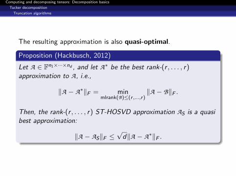
The resulting approximation is also quasi-optimal.
Proposition (Hackbusch, 2012)
Let A ∈ Fn1×···×nd , and let A∗ be the best rank-(r , . . . , r)approximation to A, i.e.,
‖A − A∗‖F = minmlrank(B)≤(r ,...,r)
‖A − B‖F .
Then, the rank-(r , . . . , r) ST-HOSVD approximation AS is a quasibest approximation:
‖A − AS‖F ≤√
d‖A − A∗‖F .
Computing and decomposing tensors: Decomposition basics
Tensor rank decomposition
Overview
1 Introduction
2 Basic tensor operations
3 Tucker decompositionMultilinear rankHigher-order singular value decompositionNumerical issuesTruncation algorithms
4 Tensor rank decompositionRankBorder rankIdentifiability
5 References
Computing and decomposing tensors: Decomposition basics
Tensor rank decomposition
Rank
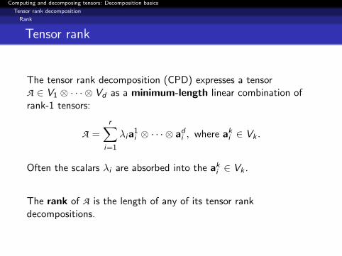
Tensor rank
The tensor rank decomposition (CPD) expresses a tensorA ∈ V1 ⊗ · · · ⊗ Vd as a minimum-length linear combination ofrank-1 tensors:
A =r∑
i=1
λia1i ⊗ · · · ⊗ ad
i , where aki ∈ Vk .
Often the scalars λi are absorbed into the aki ∈ Vk .
The rank of A is the length of any of its tensor rankdecompositions.
Computing and decomposing tensors: Decomposition basics
Tensor rank decomposition
Rank
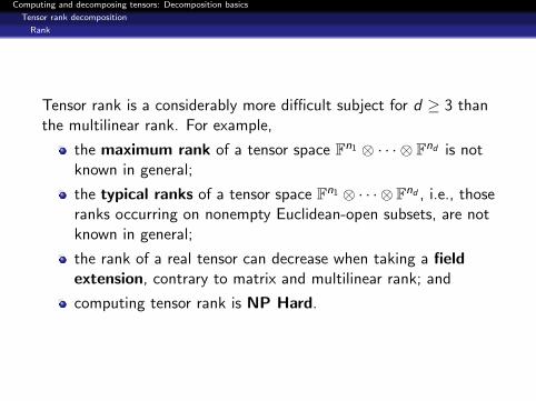
Tensor rank is a considerably more difficult subject for d ≥ 3 thanthe multilinear rank. For example,
the maximum rank of a tensor space Fn1 ⊗ · · · ⊗ Fnd is notknown in general;
the typical ranks of a tensor space Fn1 ⊗ · · · ⊗ Fnd , i.e., thoseranks occurring on nonempty Euclidean-open subsets, are notknown in general;
the rank of a real tensor can decrease when taking a fieldextension, contrary to matrix and multilinear rank; and
computing tensor rank is NP Hard.
Computing and decomposing tensors: Decomposition basics
Tensor rank decomposition
Rank
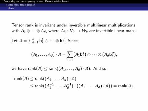
Tensor rank is invariant under invertible multilinear multiplicationswith A1⊗· · ·⊗Ad , where Ak : Vk →Wk are invertible linear maps.
Let A =∑r
i=1 b1i ⊗ · · · ⊗ bd
i . Since
(A1, . . . ,Ad) · A =r∑
i=1
(A1b1i )⊗ · · · ⊗ (Adbd
i ),
we have rank(A) ≤ rank((A1, . . . ,Ad) · A). And so
rank(A) ≤ rank((A1, . . . ,Ad) · A)
≤ rank((A−11 , . . . ,A−1
d ) ·((A1, . . . ,Ad) · A
)) = rank(A).
Computing and decomposing tensors: Decomposition basics
Tensor rank decomposition
Border rank
Overview
1 Introduction
2 Basic tensor operations
3 Tucker decompositionMultilinear rankHigher-order singular value decompositionNumerical issuesTruncation algorithms
4 Tensor rank decompositionRankBorder rankIdentifiability
5 References

Computing and decomposing tensors: Decomposition basics
Tensor rank decomposition
Border rank
Border rank
Another issue with tensor rank is that the set
S≤r := {A ∈ Fn1×···×nd | rank(A) ≤ r}
is not closed in general, i.e., S≤r 6= S≤r .
For example, for any linearly independent x, y ∈ Rn, we have
limε→0
(1
ε(x + εy)⊗3 − 1
εx⊗3
)= y⊗x⊗x+x⊗y⊗x+x⊗x⊗y;
evidently, the tensors in the sequence have rank bounded by 2, butit can be shown that the limit has rank 3.
Computing and decomposing tensors: Decomposition basics
Tensor rank decomposition
Border rank
Connection to algebraic geometry
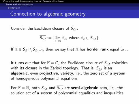
Consider the Euclidean closure of S≤r :
S≤r := { limε→0
Aε, where Aε ∈ S≤r}.
If A ∈ S≤r \S≤r−1, then we say that A has border rank equal to r .
It turns out that for F = C, the Euclidean closure of S≤r coincideswith its closure in the Zariski topology. That is, S≤r is analgebraic, even projective, variety, i.e., the zero set of a systemof homogeneous polynomial equations.
For F = R, both S≤r and S≤r are semi-algebraic sets, i.e., thesolution set of a system of polynomial equalities and inequalities.
Computing and decomposing tensors: Decomposition basics
Tensor rank decomposition
Identifiability
Overview
1 Introduction
2 Basic tensor operations
3 Tucker decompositionMultilinear rankHigher-order singular value decompositionNumerical issuesTruncation algorithms
4 Tensor rank decompositionRankBorder rankIdentifiability
5 References
Computing and decomposing tensors: Decomposition basics
Tensor rank decomposition
Identifiability
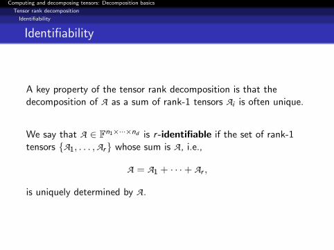
Identifiability
A key property of the tensor rank decomposition is that thedecomposition of A as a sum of rank-1 tensors Ai is often unique.
We say that A ∈ Fn1×···×nd is r-identifiable if the set of rank-1tensors {A1, . . . ,Ar} whose sum is A, i.e.,
A = A1 + · · ·+ Ar ,
is uniquely determined by A.
Computing and decomposing tensors: Decomposition basics
Tensor rank decomposition
Identifiability
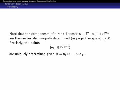
Note that the components of a rank-1 tensor A ∈ Fn1 ⊗ · · · ⊗ Fnd
are themselves also uniquely determined (in projective space) by A.Precisely, the points
[ak ] ∈ P(Fnk )
are uniquely determined given A = a1 ⊗ · · · ⊗ ad .
Computing and decomposing tensors: Decomposition basics
Tensor rank decomposition
Identifiability
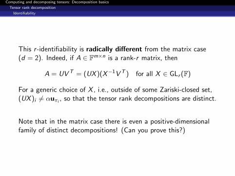
This r -identifiability is radically different from the matrix case(d = 2). Indeed, if A ∈ Fm×n is a rank-r matrix, then
A = UV T = (UX )(X−1V T ) for all X ∈ GLr (F)
For a generic choice of X , i.e., outside of some Zariski-closed set,(UX )i 6= αuπi , so that the tensor rank decompositions are distinct.
Note that in the matrix case there is even a positive-dimensionalfamily of distinct decompositions! (Can you prove this?)
Computing and decomposing tensors: Decomposition basics
Tensor rank decomposition
Identifiability
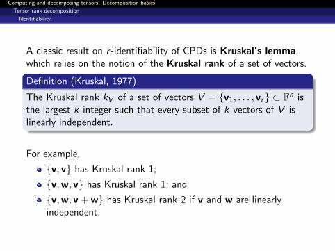
A classic result on r -identifiability of CPDs is Kruskal’s lemma,which relies on the notion of the Kruskal rank of a set of vectors.
Definition (Kruskal, 1977)
The Kruskal rank kV of a set of vectors V = {v1, . . . , vr} ⊂ Fn isthe largest k integer such that every subset of k vectors of V islinearly independent.
For example,
{v, v} has Kruskal rank 1;
{v,w, v} has Kruskal rank 1; and
{v,w, v + w} has Kruskal rank 2 if v and w are linearlyindependent.
Computing and decomposing tensors: Decomposition basics
Tensor rank decomposition
Identifiability
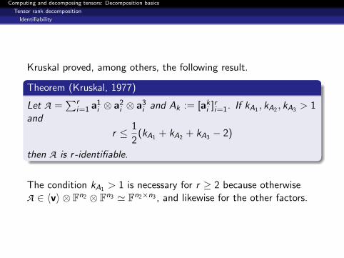
Kruskal proved, among others, the following result.
Theorem (Kruskal, 1977)
Let A =∑r
i=1 a1i ⊗ a2
i ⊗ a3i and Ak := [ak
i ]ri=1. If kA1 , kA2 , kA3 > 1and
r ≤ 1
2(kA1 + kA2 + kA3 − 2)
then A is r -identifiable.
The condition kA1 > 1 is necessary for r ≥ 2 because otherwiseA ∈ 〈v〉 ⊗ Fn2 ⊗ Fn3 ' Fn2×n3 , and likewise for the other factors.
Computing and decomposing tensors: Decomposition basics
Tensor rank decomposition
Identifiability
Computing the Kruskal rank of r vectors in Fn is very expensive, ingeneral, as one needs to compute the ranks of all
(rk
)subsets of k
vectors for k = 1, . . . ,min{r , n}. Computing one of these ranksalready has a complexity of nk2.
Notwithstanding this limitation, applying Kruskal’s lemma is apopular technique for verifying that a tensor given as the sum of rrank-1 tensors has rank equal to r . Indeed, a rank-r tensor is neverr ′-identifiable with r ′ > r .
Computing and decomposing tensors: Decomposition basics
Tensor rank decomposition
Identifiability
Kruskal’s lemma can also be applied to higher-order tensors
A ∈ V1 ⊗ · · · ⊗ Vd
simply by grouping the factors:
A ∈ (Vπ1 ⊗ · · · ⊗ Vπs )⊗ (Vπs+1 ⊗ · · · ⊗ Vπt )⊗ (Vπt+1 ⊗ · · · ⊗ Vπd )
where 1 ≤ s < t ≤ d and π is a permutation of {1, . . . , d}.
In other words, Kruskal’s lemma is applied to the reshaped tensor(coordinate array).
Computing and decomposing tensors: Decomposition basics
Tensor rank decomposition
Identifiability
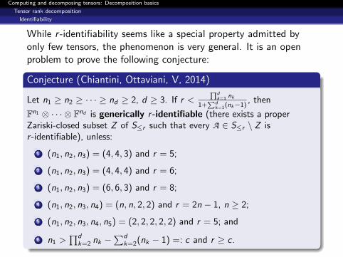
While r -identifiability seems like a special property admitted byonly few tensors, the phenomenon is very general. It is an openproblem to prove the following conjecture:
Conjecture (Chiantini, Ottaviani, V, 2014)
Let n1 ≥ n2 ≥ · · · ≥ nd ≥ 2, d ≥ 3. If r <∏d
k=1 nk1+
∑dk=1(nk−1)
, then
Fn1 ⊗ · · · ⊗ Fnd is generically r-identifiable (there exists a properZariski-closed subset Z of S≤r such that every A ∈ S≤r \ Z isr -identifiable), unless:
1 (n1, n2, n3) = (4, 4, 3) and r = 5;
2 (n1, n2, n3) = (4, 4, 4) and r = 6;
3 (n1, n2, n3) = (6, 6, 3) and r = 8;
4 (n1, n2, n3, n4) = (n, n, 2, 2) and r = 2n − 1, n ≥ 2;
5 (n1, n2, n3, n4, n5) = (2, 2, 2, 2, 2) and r = 5; and
6 n1 >∏d
k=2 nk −∑d
k=2(nk − 1) =: c and r ≥ c .
Computing and decomposing tensors: Decomposition basics
References
Overview
1 Introduction
2 Basic tensor operations
3 Tucker decompositionMultilinear rankHigher-order singular value decompositionNumerical issuesTruncation algorithms
4 Tensor rank decompositionRankBorder rankIdentifiability
5 References
Computing and decomposing tensors: Decomposition basics
References
References for basic tensor operations
Greub, Multilinear Algebra, 2nd ed., Springer, 1978.
de Silva, Lim, Tensor rank and the ill-posedness of the bestlow-rank approximation problem, SIAM Journal on MatrixAnalysis and Applications, 2008.
Kolda, Bader, Tensor decompositions and applications, SIAMReview, 2008.
Landsberg, Tensors: Geometry and Applications, AMS, 2012.
Computing and decomposing tensors: Decomposition basics
References
References for Tucker decomposition
Carlini, Kleppe, Ranks derived from multilinear maps, Journalof Pure and Applied Algebra, 2011.
De Lathauwer, De Moor, Vandewalle, A multilinear singularvalue decomposition, SIAM Journal on Matrix Analysis andApplications, 2000.
Hackbusch, Tensor Spaces and Numerical Tensor Calculus,Springer, 2012.
Hitchcock, Multiple invariants and generalized rank of aP-way matrix or tensor, Journal of Mathematics and Physics,1928.
Tucker, Some mathematical notes on three-mode factoranalysis, Psychometrika, 1966.
Vannieuwenhoven, Vandebril, Meerbergen, A new truncationstrategy for the higher-order singular value decomposition,SIAM Journal on Scientific Computing, 2012.
Computing and decomposing tensors: Decomposition basics
References
References for tensor rank decomposition
Chiantini, Ottaviani, Vannieuwenhoven, An algorithm forgeneric and low-rank specific identifiability of complex tensors,SIAM Journal on Matrix Analysis, 2014.
Chiantini, Ottaviani, Vannieuwenhoven, Effective criteria forspecific identifiability of tensors and forms, SIAM Journal onMatrix Analysis, 2017.
de Silva, Lim, Tensor rank and the ill-posedness of the bestlow-rank approximation problem, SIAM Journal on MatrixAnalysis and Applications, 2008.
Hitchcock, The expression of a polyadic or tensor as a sum ofproducts, Journal of Mathematics and Physics, 1927.
Kruskal, Three-way arrays: rank and uniqueness of trilineardecompositions, with application to arithmetic complexity andstatistics, Linear Algebra and its Applications, 1977.
Landsberg, Tensors: Geometry and Applications, AMS, 2012.


![[11] The Singular Value Decomposition · [11] The Singular Value Decomposition. The Singular Value Decomposition Gene Golub’s license plate, photographed by Professor P. M. Kroonenberg](https://cdn.vdocument.in/doc/165x107/5ff1342f977c370534443638/11-the-singular-value-decomposition-11-the-singular-value-decomposition-the.jpg)
