
© 2011 ANSYS, Inc. October 24, 20111
Simulation Advances for RF, Microwave and Antenna Applications
Presented by Martin Vogel, PhDApplication Engineer

© 2011 ANSYS, Inc. October 24, 20112
• Advanced Integrated Solver Technologies– Finite Arrays with Domain Decomposition– Hybrid solving: FEBI, IE Regions
• Physical Optics Solver in HFSS‐IE• Improved Multi‐Physics flow in Workbench
Overview

© 2011 ANSYS, Inc. October 24, 20113
Advanced Solvers:Finite Arrays with DDM

© 2011 ANSYS, Inc. October 24, 20114
Finite Arrays with Domain DecompositionEfficient solution for repeating geometries (array) with domain decomposition technique (DDM)

© 2011 ANSYS, Inc. October 24, 20115
A Review: Domain Decomposition
Distributes mesh domains to network of processors
Significantly increases simulation capacity
Highly scalable to large numbers of processors
Automatic generation of domains by mesh partitioning
• User friendly• Load balance
Distributes mesh sub-domainsto networked processors and memory

© 2011 ANSYS, Inc. October 24, 20116
Finite Antenna ArraysDefine unit cell and array
dimensions
Efficient Domain Decomposition solution
• Leverages repeating nature of array geometries
• Only mesh unit cell• Virtually repeat mesh throughout array
Post‐process full S‐parameter• Couplings included• Edge effects included
3D field visualization
Far field patterns for full array
Memory efficient Enabled with the HFSS HPC
product

© 2011 ANSYS, Inc. October 24, 20117
Finite Arrays by Domain Decomposition• Each element in array treated as solution domain
• One compute engine can solve multiple elements/domains in series
Distributes element sub-domainsto networked processors and memory

© 2011 ANSYS, Inc. October 24, 20118
Example: Skewed Waveguide Array
• 16X16 (256 elements and excitations)
• Skewed Rectangular Waveguide (WR90) Array– 1.3M Matrix Size
• Using 8 cores– 3 hrs. solution time– 0.4GB Memory total
• Using 16 cores– 2 hrs. solution time– 0.8GB Memory total
• Additional Cores– Faster solution time– More memory.
Unit cell shown with wireframe view of virtual array

© 2011 ANSYS, Inc. October 24, 20119
Skewed Waveguide Array
• Patterns from 8X8 Array– Dashed is
idealized infinite array analysis
– Solid from finite array analysis
• Two simulations use identical mesh
• Note edge effects due to finite array size

© 2011 ANSYS, Inc. October 24, 201110
Running Finite Array
Use Master/Slave unit cell design to adapt the mesh
• Called “Unit Cell for Adaptive Meshing” in image
Copy/Paste Design• Called “8X8 Array” in image
Create a single pass setup in finite array design
On “Advanced” tab use “Setup Link” to link mesh from unit cell design
Doing adaptive meshing in finite array design will be time consuming and not as efficient

© 2011 ANSYS, Inc. October 24, 201111
Efficient: 8X8 Array Patch Array
Direct solver with 12 cores• 5:05:14• 60.8 GB RAM
Finite Array DDM with 12 cores
• 00:44:53• 1.8 GB
6.8X faster33.8X less memory

© 2011 ANSYS, Inc. October 24, 201112
HPC: Faster with additional coresLinux cluster• 16X Dell PowerEdge R610
– Dual six‐core Xeon X5760, 8GB per core
Same 8X8 array of probe feed patch antennas
3M+ matrix size, 64 excitations
Study performed using 101, 51 ,26, 11, 6 and 3 engines.*• 101 simulation time = 17 min., 20X faster than direct solver• *Three engines used as baseline
1
2
3
4
5
6
7
0 50 100 150
speed factor
speed factor
Number of cores
© 2011 ANSYS, Inc. October 24, 201113
Hybrid Solving: Finite Element‐Boundary Integral

© 2011 ANSYS, Inc. October 24, 201114
• Antenna Placement Study: UHF Antenna on Apache UH64 airframe– Finite Elements with DDM– Boundary Integral (3D Method of Moments)– Hybrid Finite Element‐Boundary Integral (FE‐BI)
Finite Element‐Boundary IntegralSolving Larger Problems with Rigor

© 2011 ANSYS, Inc. October 24, 201115
Hybrid Solving: Finite Element‐ Boundary Integral
Apache helicopter• UHF antenna placement study @ 900 MHz
Solution volume• 1,250 m3
• 33,750 λ3
Solution Specs• 72 engines• Matrix size = 47M• 6 adaptive passes• 300 GB RAM• 5 hr 30 min
Finite Elements with DDM

© 2011 ANSYS, Inc. October 24, 201116
Hybrid Solving: Finite Element‐ Boundary Integral
Apache helicopter• UHF antenna placement study @ 900 MHz
Solution surface• 173 m2
• 1557 λ2
Solution Specs• 12 core MP• 680k unknowns• 9 adaptive passes• 83 GB RAM• 5 hr 28 min
Boundary Integral, 3D MoM with HFSS‐IE

© 2011 ANSYS, Inc. October 24, 201117
Hybrid Solving: Finite Element‐ Boundary Integral
Apache helicopter• UHF antenna placement study @ 900 MHz
FEM solution volume• 69 m3
• 1863 λ3
IE solution surface• 236 m2
• 2124 λ2
Solution Specs• 12 cores total using DDM with MP
• Matrix Size = 2.9M• 6 adaptive passes• 21 GB RAM• 1 hr 3 min
Hybrid Finite Element – Boundary Integral
Compared to 72 core FEM solution 14X less memory, 5.5 times faster

© 2011 ANSYS, Inc. October 24, 201118
Summary of FEBI performance
Type Time, Ratio Memory, Ratio
FEM + DDM 5hr 30min, 1 300GB, 1
IE 5hr 28min, 1 83GB, 3.6
FEBI 1hr 3min, 5.5 21 GB, 14.3

© 2011 ANSYS, Inc. October 24, 201119
FE‐BI and Distributed Solving
HPC distributes mesh sub-domains, FEM and IE domains,to networked processors and memory
FEM Domain 1
FEM Domain 2
FEM Domain 3
FEM Domain 4
IE Domain
• Distributes mesh sub‐domains to network of processors• FEM volume can be sub‐divided into multiple domains
• IE Domain is distributed to second node in machine list
• Significantly increases simulation capacity
• Multi‐processor nodes can be utilized

© 2011 ANSYS, Inc. October 24, 201120
Hybrid Solving: IE Regions

© 2011 ANSYS, Inc. October 24, 201121
FEBI and Physically Separate “Domains”Reflector with multiple FE‐BI domains• Conducting reflector and feed horn each surrounded by air with FEBI applied to surface of air volumes
• But 3D MoM solution from integral equations could be applied directly to reflector’s conducting surface only
© 2011 ANSYS, Inc. October 24, 201122
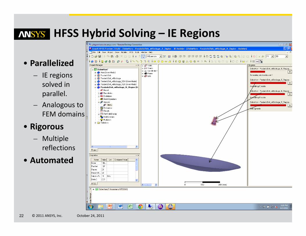
HFSS Hybrid Solving – IE Regions
• Parallelized– IE regions
solved in parallel.
– Analogous to FEM domains
• Rigorous– Multiple
reflections
• Automated

© 2011 ANSYS, Inc. October 24, 201123
HFSS IE Regions ‐ Example

© 2011 ANSYS, Inc. October 24, 201124
Physical Optics

© 2011 ANSYS, Inc. October 24, 201125
HFSS‐IE POAsymptotic solver for very large
geometries• In HFSS‐IE• Currents are approximated in illuminated regions– Set to zero in shadow regions
• No ray tracing or multiple “bounces”
Target applications:• Large reflector antennas• RCS of large objects such as satellites
Option in solution setup for HFSS‐IESourced by incident wave excitations• Plane waves or linked HFSS designs as a source

© 2011 ANSYS, Inc. October 24, 201126
Physical Optics Solver in HFSS-IE
• For illuminated surfaces Jsurf ≈2(n x Hinc ) if perfect conductor.
• For non-illuminated surfaces Jsurf ≈ 0.
• No need to solve a large matrix equation.
Where: JPO = 2(n x Hinc )
PEC

© 2011 ANSYS, Inc. October 24, 201127
PO Examples
Notice the shadowing of the gun barrel on the tank and of the tank on the ground.

© 2011 ANSYS, Inc. October 24, 201128
HFSS‐IE PO ‐ Example
Offset reflector 50 λ0 in diameter fed by a horn HFSS far field link
Simulated with 8 coresIE: 48.3min and 11.9GBPO: 23S and 286MBNote > 120x speedup

© 2011 ANSYS, Inc. October 24, 201129
ANSYS Workbench• Geometry and material transfer

© 2011 ANSYS, Inc. October 24, 201130
Ansoft to ANSYS Geometry Transfer
• Geometry and material assignment transfer from electromagnetic tools to ANSYS Thermal and Mechanical
CAD tool

© 2011 ANSYS, Inc. October 24, 201131
Highlights• New technique for finite phased‐array antennas• IE Regions• Physical Optics Solver in HFSS‐IE
• Improved Multiphysics flow


