
1
A Stochastic Differential (Difference) Game Model With an LP Subroutine for Mixed and Pure Strategy OptimizationINFORMS International Meeting 2007, Puerto Rico
Peter LohmanderProfessor
SLU Umea, SE-901 83, Sweden, http://www.Lohmander.com
Version 2007-09-29

2
Abstract: This paper presents a stochastic two person differential (difference)
game model with a linear programming subroutine that is used to optimize pure and/or mixed strategies as a function of state and time.
In ”classical dynamic models”, ”pure strategies” are often assumed to be optimal and deterministic continuous path equations can be derived. In such models, scale and timing effects in operations are however usually not considered.
When ”strictly convex scale effects” in operations with defence and attack (”counter air” or ”ground support”) are taken into consideration, dynamic mixed OR pure strategies are optimal in different states.
The optimal decision frequences are also functions of the relative importance of the results from operations in different periods.
The expected cost of forcing one participant in the conflict to use only pure strategies is determined.
The optimal responses of the opposition in case one participant in the conflict is forced to use only pure strategies are calculated.
Dynamic models of the presented type, that include mixed strategies, are highly relevant and must be used to determine the optimal strategies. Otherwise, considerable and quite unnecessary losses should be expected.
3
Inspiration:
• Isaacs R. (1965) Differential Games – A mathematical theory with applications to warfare and pursuit, control and optimization, Wiley, 1965 (Also Dover, 1999)
• Washburn, A.R. (2003) Two-person zero-sum games, 3 ed., INFORMS, Military applications society, Topics in operations research

4
Flexibility
Some resources may be used in different ways.
This is true and important in the air force, in the army and in the enterprises in the economy.

5
Our Plan to Win
This plan is focused on continuously increasing McDonald's relevance to consumers' everyday lives through multiple initiatives surrounding the five key drivers of great restaurant experiences.
Our efforts, complemented with financial discipline, have delivered for shareholders some of the strongest results in our history.

6
W-lanMax Hamburger restaurants is the only national restaurant chain to offer free Internet access for all guests. Connection is offered via W-Lan.
The most satisfied guestsFor the fith year in a row Max Hamburger Restaurants has Sweden's most satisfied customers among the national hamburger restaurants according to a new survey by SIFO/ISI Wissing.

7
BoeingB-52 StratofortressIntercontinental Strategic Bomber

8
JAS 39 Gripen
Multirole fighter

9

10
1t T
1 1( , ) 0T TV x y
1
1
0,1,...,
0,1,...,
T x
T y
x N
y N

11
t T
( , )T T T TV x y x y
0,1,...,
0,1,...,
T x
T y
x N
y N
12
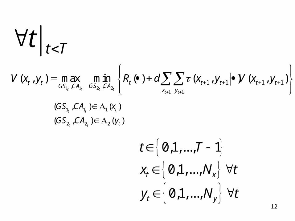
t Tt
2 21 11 1
1 1 1 1,,
( , ) max min ( ) ( , ) ( , )t tt t
t t
t t t t t t tGS CAGS CA
x y
V x y R d x y V x y
1 1 1
2 2 2
( , ) ( )
( , ) ( )t t
t t
t
t
GS CA x
GS CA y
0,1,..., 1
0,1,...,
0,1,...,
t x
t y
t T
x N t
y N t

13
1 1 2 2( ) ( , , , , , )t t t tt t t tR R GS CA GS CA x y
1 1 1 1 1 1 2 2( , ) ( , , , , , , )t t t tt t t t t tx y x y GS CA GS CA x y

14
Special case 1:
1 1
2 2
t t
t t
t
t
GS CA x
GS CA y
Special case 2:
1 1
2 2
t t
t t
t
t
GS CA x
GS CA y

15
In Model 1:
1 2
2 1
( )1 1
t t
t t
t
GS GSR
CA CA

16
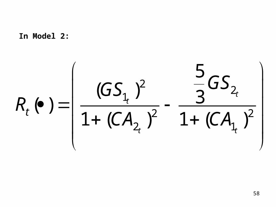
In Model 2:
22
1
2 22 1
5( ) 3( )1 ( ) 1 ( )
tt
t t
t
GSGSR
CA CA
17
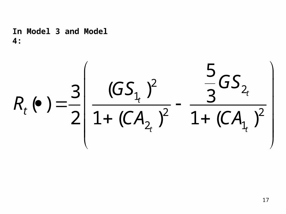
In Model 3 and Model 4:
22
1
2 22 1
5( )3 3( )
2 1 ( ) 1 ( )
tt
t t
t
GSGSR
CA CA

18
Model 1

19

20
Model 1!TAW_070611;!Peter Lohmander;Model:
sets:xset/1..3/:;yset/1..3/:;nset/1..3/:;D1set/1..3/:;D2set/1..3/:;xyset(xset,yset):;xynset(xset,yset,nset):V;xyD1set(xset,yset,D1set):GS1, CA1;xyD2set(xset,yset,D2set):GS2, CA2;xynD1s(xset,yset,nset,D1set):xdec;xD1D2s(xset, D1set, D2set):;xD1D2Xs(xset,D1set, D2set, xset):TPX;yD2D1s(yset,D2set,D1set):;yD2D1yset(yset,D2set,D1set,yset):TPY;endsets

21
max = Z;Z = @sum(xyset(x,y):V(x,y,3));
!Terminal condition: No more activities occur when n <= 1 . ;@for(xyset(x,y):V(x,y,1) = 0);

22
! The last day when activities occur, n=2, all resources should be used for GS. ;
@for(xyset(x,y):V(x,y,2) = x-y);

23
! Day n >= 3, you may use some resources for GS and some for CA. The rows and columns represent the resources used for GS. ; @for(xyD1set(x,y,D1)|D1 #LE# x: GS1(x,y,D1) = D1-1 );@for(xyD1set(x,y,D1)|D1 #GT# x: GS1(x,y,D1) = 0 );
@for(xyD1set(x,y,D1): CA1(x,y,D1) = x - 1 - GS1(x,y,D1) );
@for(xyD2set(x,y,D2)|D2 #LE# y: GS2(x,y,D2) = D2-1 );@for(xyD2set(x,y,D2)|D2 #GT# y: GS2(x,y,D2) = 0 );
@for(xyD2set(x,y,D2): CA2(x,y,D2) = y - 1 - GS2(x,y,D2));

24
@for(xynset(x,y,n): @sum(D1set(D1):xdec(x,y,n,D1)) = 1);
@for(xynD1s(x,y,n,D1)| D1#GT#x: xdec(x,y,n,D1) = 0);
25
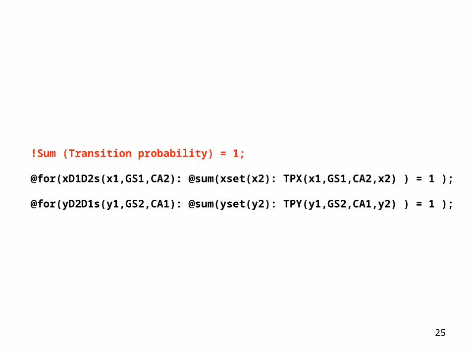
!Sum (Transition probability) = 1;
@for(xD1D2s(x1,GS1,CA2): @sum(xset(x2): TPX(x1,GS1,CA2,x2) ) = 1 );
@for(yD2D1s(y1,GS2,CA1): @sum(yset(y2): TPY(y1,GS2,CA1,y2) ) = 1 );

26
!********************************************;! Transition probability calculations for x ;!********************************************;
! Transition probabilities for x if x1 = 0;@for(xD1D2s(x1,GS1P1,CA2P1)|x1#EQ#1 : TPX(x1,GS1P1,CA2P1,x1) = 1 );
! Transition probabilities for x if CA2 = 0;@for(xD1D2s(x1,GS1P1,CA2P1)|CA2P1 #EQ# 1 : TPX(x1,GS1P1,CA2P1,x1) = 1 );
! Transition probabilities for x if GS1 = 0;@for(xD1D2s(x1,GS1P1,CA2P1)|GS1P1 #EQ# 1 : TPX(x1,GS1P1,CA2P1,x1) = 1 );

27
! Transition probabilities for x if GS1 >= 1 and CA2 = 1;
@for(xD1D2s(x1,GS1P1,CA2P1)|x1#GE#2 #AND# GS1P1#GE#2 #AND# CA2P1#EQ#2 : TPX(x1,GS1P1,CA2P1,x1) = 1/2 );
@for(xD1D2s(x1,GS1P1,CA2P1)|x1#GE#2 #AND# GS1P1#GE#2 #AND# CA2P1#EQ#2 : TPX(x1,GS1P1,CA2P1,x1-1) = 1/2 );

28
! Transition probabilities for x if GS1 = 1 and CA2 = 2; @for(xD1D2s(x1,GS1P1,CA2P1)|x1#GE#2 #AND# GS1P1#EQ#2 #AND# CA2P1 #EQ# 3 : TPX(x1,GS1P1,CA2P1,x1) = 1/4 );
@for(xD1D2s(x1,GS1P1,CA2P1)|x1#GE#2 #AND# GS1P1#EQ#2 #AND# CA2P1 #EQ# 3 : TPX(x1,GS1P1,CA2P1,x1-1) = 3/4 );

29
! Transition probabilities for x if GS1 >= 2 and CA2 = 2; @for(xD1D2s(x1,GS1P1,CA2P1)|x1#GE#3 #AND# GS1P1#GE#3 #AND# CA2P1 #EQ# 3 : TPX(x1,GS1P1,CA2P1,x1) = 1/4 );
@for(xD1D2s(x1,GS1P1,CA2P1)|x1#GE#3 #AND# GS1P1#GE#3 #AND# CA2P1 #EQ# 3 : TPX(x1,GS1P1,CA2P1,x1-1) = 1/2 );
@for(xD1D2s(x1,GS1P1,CA2P1)|x1#GE#3 #AND# GS1P1#GE#3 #AND# CA2P1 #EQ# 3 : TPX(x1,GS1P1,CA2P1,x1-2) = 1/4 );

30
!*******************************************;! Transition probability calculations for y ;!*******************************************;
! Transition probabilities for y if y1 = 0;@for(yD2D1s(y1,GS2P1,CA1P1)|y1#EQ#1 : TPY(y1,GS2P1,CA1P1,y1) = 1 );
! Transition probabilities for y if CA1 = 0;@for(yD2D1s(y1,GS2P1,CA1P1)|CA1P1 #EQ# 1 : TPY(y1,GS2P1,CA1P1,y1) = 1 );
! Transition probabilities for y if GS2 = 0;@for(yD2D1s(y1,GS2P1,CA1P1)|GS2P1 #EQ# 1 : TPY(y1,GS2P1,CA1P1,y1) = 1 );

31
! Transition probabilities for y if GS2 >= 1 and CA1 = 1;
@for(yD2D1s(y1,GS2P1,CA1P1)|y1#GE#2 #AND# GS2P1#GE#2 #AND# CA1P1#EQ#2 : TPY(y1,GS2P1,CA1P1,y1) = 1/2 );
@for(yD2D1s(y1,GS2P1,CA1P1)|y1#GE#2 #AND# GS2P1#GE#2 #AND# CA1P1#EQ#2 : TPY(y1,GS2P1,CA1P1,y1-1) = 1/2 );

32
! Transition probabilities for y if GS2 = 1 and CA1 = 2;
@for(yD2D1s(y1,GS2P1,CA1P1)|y1#GE#2 #AND# GS2P1#EQ#2 #AND# CA1P1#EQ#3 : TPY(y1,GS2P1,CA1P1,y1) = 1/4 );
@for(yD2D1s(y1,GS2P1,CA1P1)|y1#GE#2 #AND# GS2P1#EQ#2 #AND# CA1P1#EQ#3 : TPY(y1,GS2P1,CA1P1,y1-1) = 3/4 );

33
! Transition probabilities for y if GS2 >= 2 and CA1 = 2; @for(yD2D1s(y1,GS2P1,CA1P1)|y1#GE#3 #AND# GS2P1#GE#3 #AND# CA1P1 #EQ# 3 : TPY(y1,GS2P1,CA1P1,y1) = 1/4 );
@for(yD2D1s(y1,GS2P1,CA1P1)|y1#GE#3 #AND# GS2P1#GE#3 #AND# CA1P1 #EQ# 3 : TPY(y1,GS2P1,CA1P1,y1-1) = 1/2 );
@for(yD2D1s(y1,GS2P1,CA1P1)|y1#GE#3 #AND# GS2P1#GE#3 #AND# CA1P1 #EQ# 3 : TPY(y1,GS2P1,CA1P1,y1-2) = 1/4 );

34
In Model 1:
1 2
2 1
( )1 1
t t
t t
t
GS GSR
CA CA

35
In Model 3 and Model 4:
22
1
2 22 1
5( )3 3( )
2 1 ( ) 1 ( )
tt
t t
t
GSGSR
CA CA
36
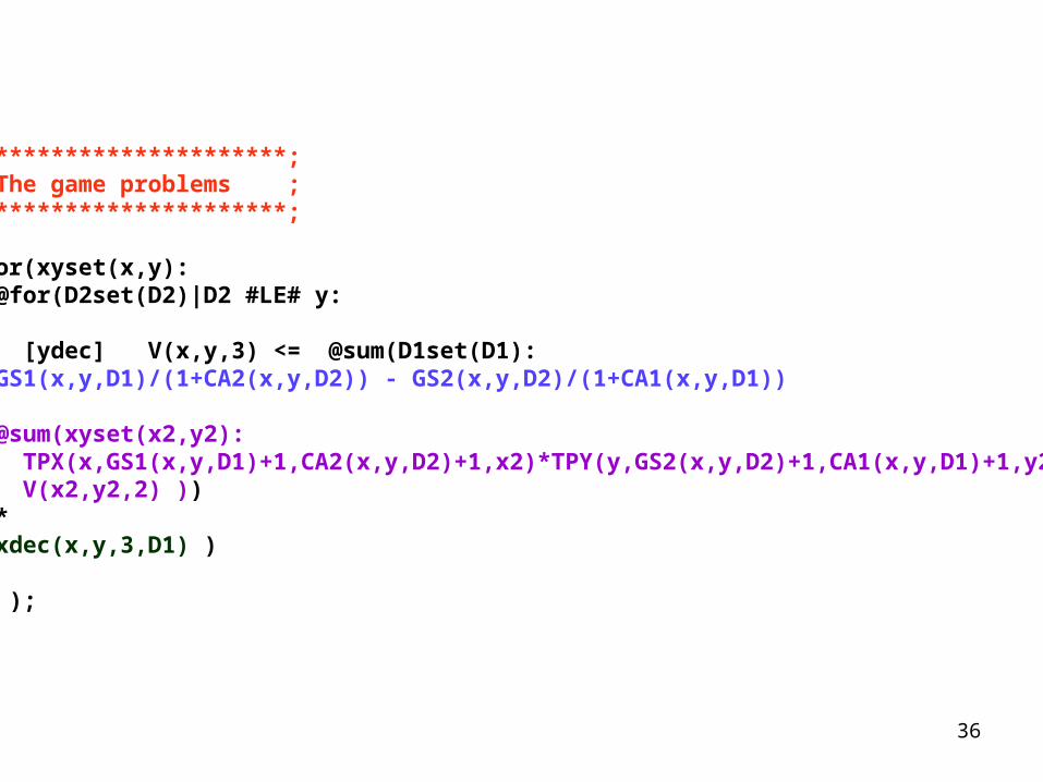
!**********************;! The game problems ;!**********************;
@for(xyset(x,y): @for(D2set(D2)|D2 #LE# y:
[ydec] V(x,y,3) <= @sum(D1set(D1): (GS1(x,y,D1)/(1+CA2(x,y,D2)) - GS2(x,y,D2)/(1+CA1(x,y,D1)) + @sum(xyset(x2,y2): TPX(x,GS1(x,y,D1)+1,CA2(x,y,D2)+1,x2)*TPY(y,GS2(x,y,D2)+1,CA1(x,y,D1)+1,y2)* V(x2,y2,2) )) * xdec(x,y,3,D1) ) ););

37
@for(xynset(x,y,n): @FREE(V(x,y,n)));
end

38
In Model 3 and Model 4:
22
1
2 22 1
5( )3 3( )
2 1 ( ) 1 ( )
tt
t t
t
GSGSR
CA CA

39
Model 3; (x,y,t) = (2,2,T-1)
GS2 = 0CA2 = 2
GS2 = 1CA2 = 1
GS2 = 2CA2 = 0
GS1 = 0CA1 = 2
3/2*(0-0)+ 0 = 0
3/2*(0 – (5/3)/(1+4)) + 0.25*(0) + 0.75*(+1) = 0.25
3/2*(0 – (5/3)*2/(1+4))+0.25*(0) + 0.5*(1) + 0.25*(2)= 0
GS1 = 1CA1 = 1
3/2*(1/(1+4)-0) +0.25*(0) + 0.75*(-1) = -0.45
3/2*(1/(1+1) – (5/3)/(1+1))+0.5*(0)+0.25*(1) + 0.25*(-1)= -0.5
3/2*(1/(1+0) – (5/3)*2/(1+1))+0.5*(0) + 0.5*(1) = -0.5
GS1 = 2CA1 = 0
3/2*(4/(1+4) – 0)+0.25*(0) + 0.5*(-1) + 0.25*(-2) = 0.2
3/2*(4/(1+1) – (5/3)/(1+0))+0.5*(0) + 0.5*(-1)= 0
3/2*(4/(1+0)-(5/3)*2/(1+0))+ 0= 1

40
Model 3; (x,y,t) = (2,2,T-1)
GS2 = 0CA2 = 2
GS2 = 1CA2 = 1
GS2 = 2CA2 = 0
GS1 = 0CA1 = 2
0
0.25 0
GS1 = 1CA1 = 1
-0.45 -0.5
-0.5
GS1 = 2CA1 = 0 0.2 0 1

41
11 12 1
21 22 2
1 2
.
.
. . . .
.
n
n
m m mn

42
1 1 1
1
.
. . .
.
n
m m n
x y x y
x y x y

43
11 1 1 1
12 1 2 2
1 1
1
max
. .
... ( )
... ( )
.
... ( )
1 ........
m m
m m
n mn m n
m
E
s t
E x x against
E x x against
E x x against
x x

44
11 1 1 1
21 1 2 2
1 1
1
min
. .
... ( )
... ( )
.
... ( )
1 ........
n n
n n
m mn n m
n
E
s t
E y y against
E y y against
E y y against
y y

45
Results from Model 1

46
Table 1.1
V(x,y,3) with Model 1(This (n=3) means that t =T-1 since we use backward recursion and period T+1 is defined as n=1. )
-4 -1.5 0
-2 0 1.5
0 2 4

47

48
(0,2) (0,2) (0,0)
(0,1) (1,1) (2,0)
(0,0) (1,0) (2,0)
Table 1.2(GS1*, GS2*) at n=3 with Model 1

49
(0,2) (0,2) (0,0)
(0,1) (1,1) (2,0)
(0,0) (1,0) (2,0)
Table 1.2(GS1*, GS2*) at n=3 with Model 1

50

51
(0,2) (0,2) (0,0)
(0,1) (1,1) (2,0)
(0,0) (1,0) (2,0)
Table 1.2(GS1*, GS2*) at n=3 with Model 1

52

53
(0,2) (0,2) (0,0)
(0,1) (1,1) (2,0)
(0,0) (1,0) (2,0)
Table 1.2(GS1*, GS2*) at n=3 with Model 1

54

55
(0,2) (0,2) (0,0)
(0,1) (1,1) (2,0)
(0,0) (1,0) (2,0)
Table 1.2(GS1*, GS2*) at n=3 with Model 1

56

57
Model 2
58
In Model 2:
22
1
2 22 1
5( ) 3( )1 ( ) 1 ( )
tt
t t
t
GSGSR
CA CA

59
Model 2
!**********************;! The game problems ;!**********************;
@for(xyset(x,y): @for(D2set(D2)|D2 #LE# y: [ydec] V(x,y,3) <= @sum(D1set(D1):
(GS1(x,y,D1)*GS1(x,y,D1)/(1+CA2(x,y,D2)*CA2(x,y,D2)) - 5/3*GS2(x,y,D2)/(1+CA1(x,y,D1)*CA1(x,y,D1)) + @sum(xyset(x2,y2): TPX(x,GS1(x,y,D1)+1,CA2(x,y,D2)+1,x2)*TPY(y,GS2(x,y,D2)+1,CA1(x,y,D1)+1,y2)* V(x2,y2,2) )) * xdec(x,y,3,D1) ) ););

60
Results from Model 2
61
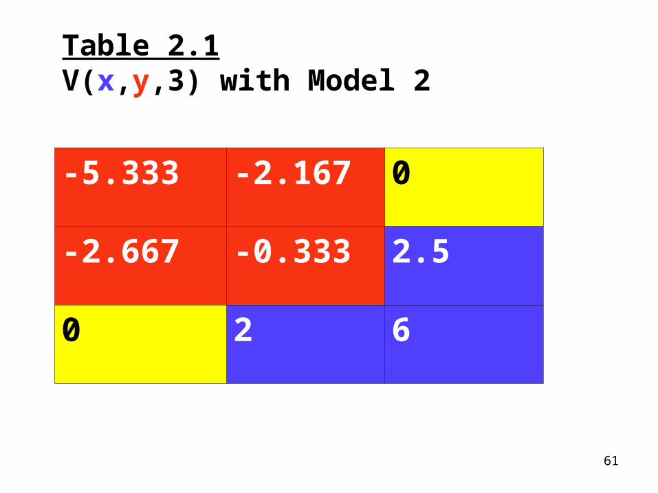
Table 2.1V(x,y,3) with Model 2
-5.333 -2.167 0
-2.667 -0.333 2.5
0 2 6
62
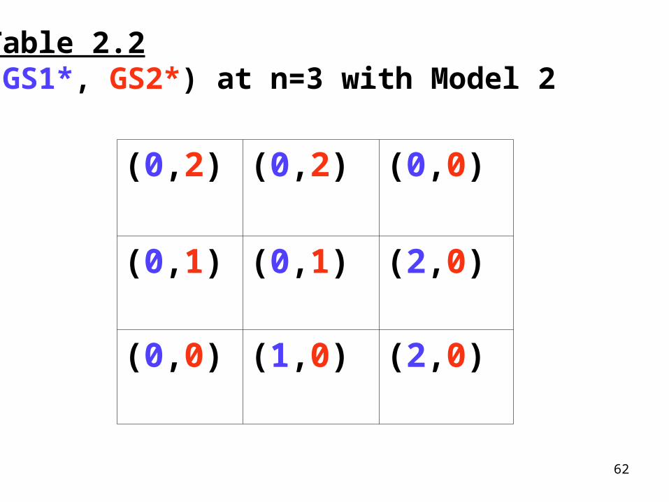
Table 2.2(GS1*, GS2*) at n=3 with Model 2
(0,2) (0,2) (0,0)
(0,1) (0,1) (2,0)
(0,0) (1,0) (2,0)

63
Table 2.2(GS1*, GS2*) at n=3 with Model 2
(0,2) (0,2) (0,0)
(0,1) (0,1) (2,0)
(0,0) (1,0) (2,0)

64

65
Model 3

66
In Model 3 and Model 4:
22
1
2 22 1
5( )3 3( )
2 1 ( ) 1 ( )
tt
t t
t
GSGSR
CA CA

67
!**********************;! The game problems ;!**********************;
@for(xyset(x,y): @for(D2set(D2)|D2 #LE# y: [ydec] V(x,y,3) <= @sum(D1set(D1):
( 3/2*(GS1(x,y,D1)*GS1(x,y,D1)/(1+CA2(x,y,D2)*CA2(x,y,D2)) - 5/3*GS2(x,y,D2)/(1+CA1(x,y,D1)*CA1(x,y,D1)) ) !A constant is added and later removed; + (1 +)
@sum(xyset(x2,y2): TPX(x,GS1(x,y,D1)+1,CA2(x,y,D2)+1,x2)*TPY(y,GS2(x,y,D2)+1,CA1(x,y,D1)+1,y2)* V(x2,y2,2) )) * xdec(x,y,3,D1) ) ););

68
Results from Model 3

69
Table 3.1V(x,y,3) with Model 3
-7 -3 0.111
-3.5 -0.75 3.5
0 2.5 8

70
Table 3.2(GS1*, GS2*) at n=3 with Model 3
(0,2) (0,2) (0,0) Prob = .4444444 * .5555556 = .246914
(2,0) Prob = .5555556 * .5555556 = .308642
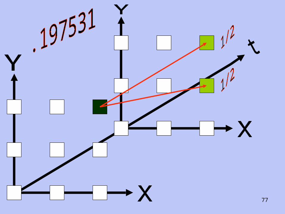
(0,1) Prob = .4444444 * .4444444 = .197531
(2,1) Prob = .5555556 * .4444444 = .246914 Sum = 1.000001
(0,1) (0,1) (2,0)
(0,0) (1,0) (2,0)
71
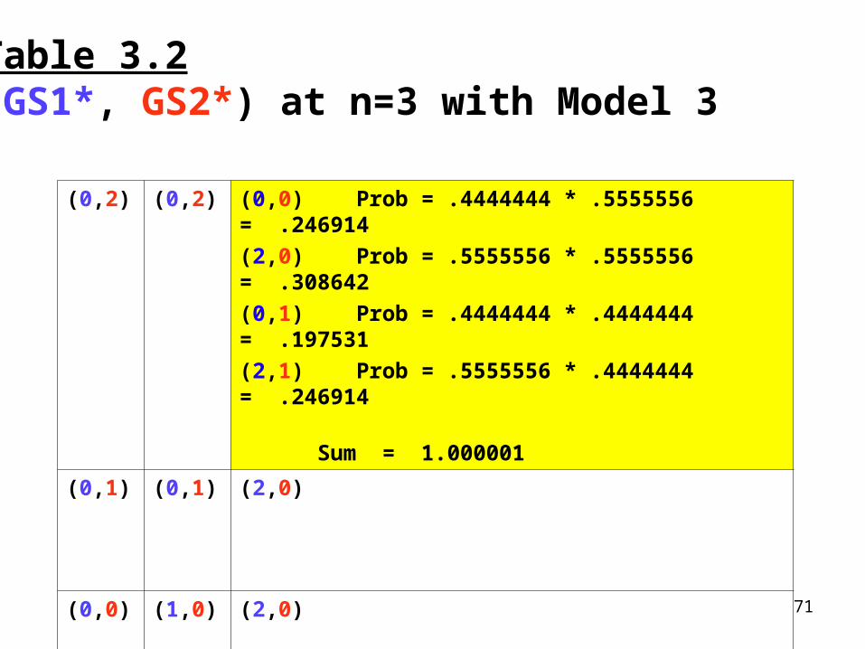
Table 3.2(GS1*, GS2*) at n=3 with Model 3
(0,2) (0,2) (0,0) Prob = .4444444 * .5555556 = .246914
(2,0) Prob = .5555556 * .5555556 = .308642
(0,1) Prob = .4444444 * .4444444 = .197531
(2,1) Prob = .5555556 * .4444444 = .246914 Sum = 1.000001
(0,1) (0,1) (2,0)
(0,0) (1,0) (2,0)

72
Table 3.2(GS1*, GS2*) at n=3 with Model 3
(0,2) (0,2) (0,0) Prob = .4444444 * .5555556 = .246914
(2,0) Prob = .5555556 * .5555556 = .308642
(0,1) Prob = .4444444 * .4444444 = .197531
(2,1) Prob = .5555556 * .4444444 = .246914 Sum = 1.000001
(0,1) (0,1) (2,0)
(0,0) (1,0) (2,0)

73

74
Table 3.2(GS1*, GS2*) at n=3 with Model 3
(0,2) (0,2) (0,0) Prob = .4444444 * .5555556 = .246914
(2,0) Prob = .5555556 * .5555556 = .308642
(0,1) Prob = .4444444 * .4444444 = .197531
(2,1) Prob = .5555556 * .4444444 = .246914 Sum = 1.000001
(0,1) (0,1) (2,0)
(0,0) (1,0) (2,0)

75

76
Table 3.2(GS1*, GS2*) at n=3 with Model 3
(0,2) (0,2) (0,0) Prob = .4444444 * .5555556 = .246914
(2,0) Prob = .5555556 * .5555556 = .308642
(0,1) Prob = .4444444 * .4444444 = .197531
(2,1) Prob = .5555556 * .4444444 = .246914 Sum = 1.000001
(0,1) (0,1) (2,0)
(0,0) (1,0) (2,0)
77

78
Table 3.2(GS1*, GS2*) at n=3 with Model 3
(0,2) (0,2) (0,0) Prob = .4444444 * .5555556 = .246914
(2,0) Prob = .5555556 * .5555556 = .308642
(0,1) Prob = .4444444 * .4444444 = .197531
(2,1) Prob = .5555556 * .4444444 = .246914 Sum = 1.000001
(0,1) (0,1) (2,0)
(0,0) (1,0) (2,0)

79

80
Model 4

81
In Model 3 and Model 4:
22
1
2 22 1
5( )3 3( )
2 1 ( ) 1 ( )
tt
t t
t
GSGSR
CA CA

82
!**********************;! The game problems ;!**********************;
@for(xyset(x,y): @for(D2set(D2)|D2 #LE# y: [ydec] V(x,y,3) <= @sum(D1set(D1):
( 3/2*(GS1(x,y,D1)*GS1(x,y,D1)/(1+CA2(x,y,D2)*CA2(x,y,D2)) - 5/3*GS2(x,y,D2)/(1+CA1(x,y,D1)*CA1(x,y,D1)) )
+ 1 + .85 *
@sum(xyset(x2,y2): TPX(x,GS1(x,y,D1)+1,CA2(x,y,D2)+1,x2)*TPY(y,GS2(x,y,D2)+1,CA1(x,y,D1)+1,y2)* V(x2,y2,2) )) * xdec(x,y,3,D1) ) ););
Note that “discounting” has been introduced!

83
Results from Model 4

84
Table 4.1V(x,y,3) with Model 4
-6.7 -2.925 0.117
-3.35 -0.825 3.425
0 2.35 7.7

85
Table 4.2(GS1*, GS2*) at n=3 with Model 4
(0,2) (0,2) (0,0) Prob = .6666667 * .1515152 = .101010
(2,0) Prob = .3333333 * .1515152 = .050505
(0,1) Prob = .6666667 * .8484849 = .565657
(2,1) Prob = .3333333 * .8484849 = .282828
Sum = 1.000000
(0,1) (0,1) (2,0)
(0,0) (1,0) (2,0)

86
Detailed study of optimal strategies:
( , , ) (2,2, 1)t tx y t T Optimal strategies with Model 3(In Model 3, future results are not discounted. d = 1)
P1:
Strategy Probability
Full CA 0.4444444
Full GS 0.5555556
P2:
Strategy Probability
Full CA 0.5555556
50% CA &50% GS
0.4444444

87
Detailed study of optimal strategies:
( , , ) (2,2, 1)t tx y t T Optimal strategies with Model 4(In Model 3, future results are not discounted. d = 0.85)
P1: P2:
Strategy Probability
Full CA 2/3
Full GS 1/3
Strategy Probability
Full CA 0.1515152
50% CA &50% GS
0.8484848

88
When the importance of instant results in relation to future results increases (= when the discounting of future results increases from 0 to 15%):
P1 increases the probability of instant full CA.P1 decreases the probability of instant GS.
P2 decreases the probability of instant full CA.P2 increases the probability of partial CA and partial GS.

89
Observations:
• Even in case there is just one more period of conflict ahead of us and even if the participants only have two units available per participant, we find that the optimal strategies are mixed.
• The optimal decision frequencies are affected by the result discounting.
• The different participants should optimally change the strategies in qualitatively different ways when the degree of discounting changes.

90
Observations cont.:
• Differential games in continuous time can not describe these mixed strategies.
• Furthermore, even if we would replace deterministic differential games in continuous time by “stochastic differential games” based on stochastic differential equations in continuous time, this would not capture the real situation, since the optimal frequencies are results of the scales of missions.
• Two resource units used during one time interval will not give the same result as one resource unit during two time intervals.

91
Isaacs (1965), in section 5.4, The war of attrition and attack:
“The realistic execution of the strategies would comprise of a series of discrete decisions. But we shall smooth matters into a continuous process. Such is certainly no farther from truth than our assumptions and therefore can be expected to be as reliable as a stepped model. It is also more facile to handle and yields general results more readily.”

92
Isaacs (1965), page 66:
• ”Similarily, except possibly on singular surfaces, the optimal strategies will be continuous functions denoted by ... when they are unique; when they are not, we shall often assume such continuous functions can be selected.”
Observation (Lohmander):• With economies of scale in operations, the optimal
strategies will usually not be continuous functions!

93
V
u
0 1 2
0
1
2
3
4 X=2
X=1
X=0

94
V*
x
0 1 2
0
1
2
3
4

95
u*(x)
x
0 1 2
0
1
2
3
4

96
Isaacs (1965) obtains differential equations that describe the optimal decisions over time by the two participants:
1 1 1 2
2 2 2 1
x m c x
x m c x
The system moves according to these equations:
97
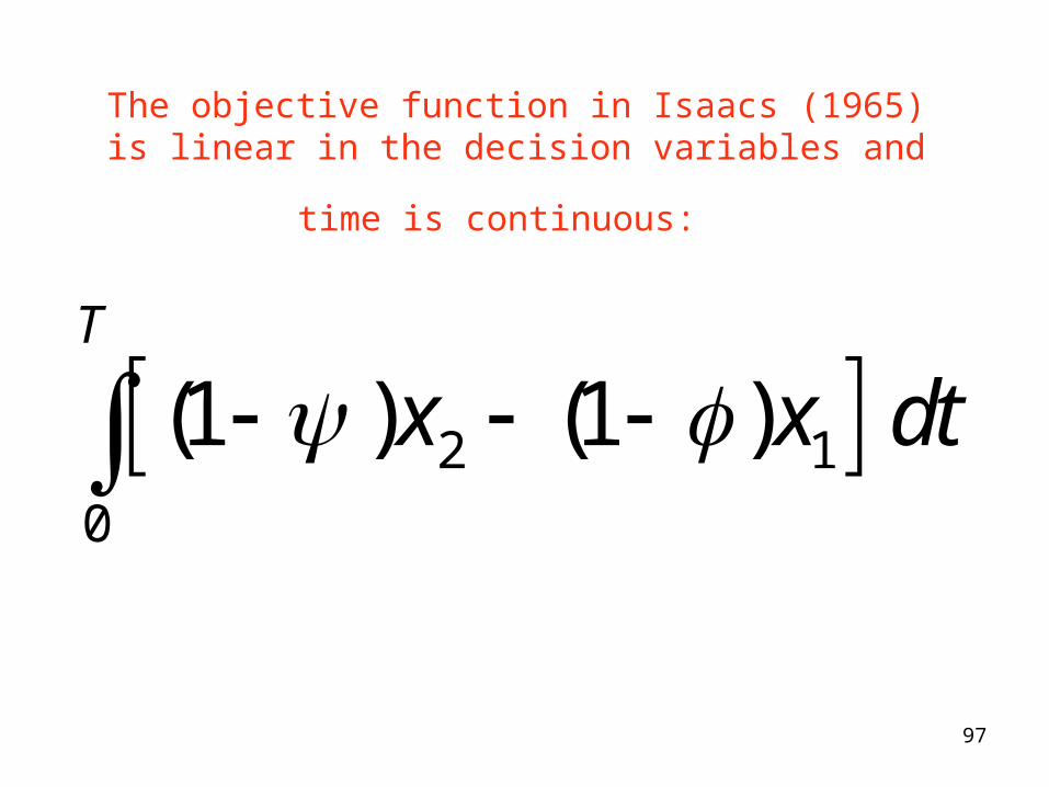
The objective function in Isaacs (1965) is linear in the
decision variables and time is continuous:
2 1
0
(1 ) (1 )T
x x dt

98
There is no reason to expect that the Isaacs (1965) model would lead to
mixed strategies. • The objective function is linear.
• Furthermore there are no scale effects in the “dynamic transition”.

99
Washburh (2003), Tactical air war:
”- It is a curious fact that in no case is a mixed strategy ever needed; in fact, in all cases each player assigns either all or none of his air force to GS.”
(The model analysed by Washburn has very strong similarities to the model analysed here. The Washburn model was even the starting point in the development of this model. However, the objective function used by Washburn is linear. Hence, the results become quite different.)

100
An analogy to optimal control:
The following observations are typical when optimal management of natural resources is investigated:
• If the product price is a constant or a decreasing function of the production and sales volume and if the cost of extraction is a strictly convex function of the extraction volume, the objective function is strictly concave in the production volume. Then we obtain a smooth differentiable optimal time path of the resource stock.
• However, if the extraction cost is concave, which is sometimes
the case if you have considerable set up costs or other scale advantages, then the optimal strategy is usually “pulse harvesting”. In this case, the objective function that we are maximizing is convex in the decision variable. The optimal stock level path then becomes non differentiable.

101
Technology differences:
• The reason why the two participants should make different decisions with different strategies is that they have different “GS-technologies”. These technologies have different degree of convexity of results with respect to the amount of resources used.
• Such differences are typical in real conflicts. They are caused by differences in equipment and applied methods. Of course, in most cases we can expect that the applied methods are adapted to the equipment and other relevant conditions.

102
• For P1, the instant GS result is strictly convex in the number of units devoted to the GS mission.
• For P2, the instant GS result is proportional to the number of units devoted to the GS mission.

103
Model 5

104
Model 5 corresponds to Model 3 but the following line is addedjust before “end”.
Case 1:xdec(3,3,3,1) = 1;
Case 2:xdec(3,3,3,2) = 1;
Case 3:xdec(3,3,3,3) = 1;

105
Results from Model 5

106
Results if the decisions of P1 are not constrained in (2,2) when n = 3 (Model 3):
Case 0:xdec(3,3,3,1) = 0.4444444 xdec(3,3,3,3) = 0.5555556 ;
(GS1 = 0 and CA1 = 2 or GS1 = 2 and CA1 = 0 )
Effects:
The value of the game : V(3,3) = 0.111
The opposition should use a mixed strategy:
GS2 = 0, CA2 = 2 with probability 0.5555556 GS2=1, CA2 = 1 with probability 0.4444444.

107
Results if the decisions of P1 are constrained in (2,2) when n = 3:
Case 1:xdec(3,3,3,1) = 1;
(GS1 = 0 and CA1 = 2 )
Effects:
The value of the game decreases: V(3,3) = 0
The decision of the opposition changes: GS2 = 2, CA2 = 0

108
Results if the decisions of P1 are constrained in (2,2) when n = 3:
Case 2:xdec(3,3,3,2) = 1;
(GS1 = 1 and CA1 =1 )
Effects:
The value of the game decreases: V(3,3) = -0.5
The decision of the opposition changes: GS2 = 2, CA2 = 0

109
Results if the decisions of P1 are constrained in (2,2) when n = 3:
Case 3:xdec(3,3,3,3) = 1;
(GS1 = 2 and CA1 = 0 )
Effects:
The value of the game decreases: V(3,3) = 0
The decision of the opposition changes: GS2 = 1, CA2 = 1

110
Conclusions from Model 5:
Since we are interested in the best attainable expected outcome,
we should not restrict our decisions to a pure strategy and let the opposition select strategy without such restrictions!
You should avoid being predictable!

111
Conclusions: This paper presents a stochastic two person differential (difference)
game model with a linear programming subroutine that is used to optimize pure and/or mixed strategies as a function of state and time.
In ”classical dynamic models”, ”pure strategies” are often assumed to be optimal and deterministic continuous path equations can be derived. In such models, scale and timing effects in operations are however usually not considered.
When ”strictly convex scale effects” in operations with defence and attack (”counter air” or ”ground support”) are taken into consideration, dynamic mixed OR pure strategies are optimal in different states.
The optimal decision frequences are also functions of the relative importance of the results from operations in different periods.
The expected cost of forcing one participant in the conflict to use only pure strategies is determined.
The optimal responses of the opposition in case one participant in the conflict is forced to use only pure strategies are calculated.
Dynamic models of the presented type, that include mixed strategies, are highly relevant and must be used to determine the optimal strategies. Otherwise, considerable and quite unnecessary losses should be expected.

112
Contact: Peter Lohmander
Professor
SLU
SE-901 83 Umea, Sweden
e-mail:
Home page:
http://www.Lohmander.com
113
Source: Lohmander, P., TAW models 070612.doc


