
1
Frequency-domain Compressive Channel
Estimation for Frequency-selective Hybrid
mmWave MIMO Systems
Javier Rodrıguez-Fernandez†, Nuria Gonzalez-Prelcic†, Kiran Venugopal‡, and
Robert W. Heath Jr.‡
† Universidade de Vigo, Email: jrodriguez,[email protected]‡ The University of Texas at Austin, Email: kiranv,[email protected]
Abstract
Channel estimation is useful in millimeter wave (mmWave) MIMO communication systems. Chan-
nel state information allows optimized designs of precoders and combiners under different metrics such
as mutual information or signal-to-interference-noise (SINR) ratio. At mmWave, MIMO precoders and
combiners are usually hybrid, since this architecture provides a means to trade-off power consumption
and achievable rate. Channel estimation is challenging when using these architectures, however, since
there is no direct access to the outputs of the different antenna elements in the array. The MIMO channel
can only be observed through the analog combining network, which acts as a compression stage of the
received signal. Most of prior work on channel estimation for hybrid architectures assumes a frequency-
flat mmWave channel model. In this paper, we consider a frequency-selective mmWave channel and
propose compressed-sensing-based strategies to estimate the channel in the frequency domain. We
evaluate different algorithms and compute their complexity to expose trade-offs in complexity-overhead-
performance as compared to those of previous approaches.
This work was partially funded by the Agencia Estatal de Investigacin (Spain) and the European Regional Development
Fund (ERDF) under project MYRADA (TEC2016-75103-C2-2-R), the U.S. Department of Transportation through the Data-
Supported Transportation Operations and Planning (D-STOP) Tier 1 University Transportation Center, by the Texas Department
of Transportation under Project 0-6877 entitled Communications and Radar-Supported Transportation Operations and Planning
(CAR-STOP) and by the National Science Foundation under Grant NSF-CCF-1319556 and NSF-CCF-1527079.
arX
iv:1
704.
0857
2v1
[cs
.IT
] 2
7 A
pr 2
017

2
Index Terms
Wideband channel estimation; millimeter wave MIMO; hybrid architecture.
I. INTRODUCTION
MIMO architectures with large arrays are a key ingredient of mmWave communication sys-
tems, providing gigabit-per-second data rates [1]. Hybrid MIMO structures have been proposed
to operate at mmWave because the cost and power consumption of an all-digital achitecture
is prohibitive at these frequencies [2]. Optimally configuring the digital and analog precoders
and combiners requires channel knowledge when the design goal is maximizing metrics such as
the achievable rate or the SINR. Acquiring the mmWave channel is challenging with a hybrid
architecture, however, because the channel is seen through the analog combining network, the
SNR is low before beamforming, and the size of the channel matrices is large [3].
A significant number of papers have proposed solutions to the problem of channel estimation
at mmWave with hybrid architectures, but under a frequency-flat channel model [4]–[12]. These
strategies exploit the spatially sparse structure in the mmWave MIMO channel, formulating the
estimation of the channel as a sparse recovery problem. The support of the estimated sparse
vector identifies the pairs of direction-of-arrival/direction-of-departure (DoA/DoD) for each path
in the mmWave channel, while the amplitudes of the non-zero coefficients provide the channel
gains for each path. Compressive estimations lead to a reduction in the channel training length
when compared to conventional approaches such as those based on least squares (LS) estimation
[12].
Recently, some approaches for channel estimation in frequency-selective mmWave channels
have been proposed. In a recent paper [13], we designed a time-domain approach to estimate
the wideband mmWave channel assuming a hybrid MIMO architecture. This algorithm exploits
the sparsity of the wideband millimeter wave channel in both the angular and delay domains.
The sparse formulation of the problem in [13] includes the effect of non-integer sampling of the
transmit pulse shaping filter, with the subsequent leakage effect and increase of sparsity level
in the channel matrix. The main limitation of [13] is that the algorithm can be applied only to
single carrier systems. A frequency-domain strategy to estimate frequency-selective mmWave
channels was also proposed in [14]. A sparse reconstruction problem was formulated there to
3
estimate the channel independently for every subcarrier, without exploiting spatial congruence
between subbands. Another approach in the frequency domain was designed in [15], but only
exploting the information from a reduced number of subcarriers. A different algorithm operating
in the frequency domain for a MIMO-OFDM system was proposed in [16]. Exploiting the fact
that spatial propagation characteristics do not change significantly within the system bandwidth,
[16] assumed spatially common sparsity between the channels corresponding to the different
subcarriers. A structured sparse recovery algorithm was then considered to reconstruct the
channels in the frequency domain. Thus, [16] is an interesting initial solution to the problem,
but has several limitations when applied to a mmWave communication system:
1) The effect of sampling the pulse shaping filter delayed by a non integer factor was not
considered in the channel model for a given delay tap. As shown in [18], not accounting
for this effect leads to virtual MIMO matrices with an artificially enhanced sparsity.
2) The algorithm was evaluated only for medium and high SNR regimes (larger than 10 dBs),
very unlikely at mmWave, where the expected SNR is below 0 dB.
3) The reconstruction algorithm provides accurate results when Gaussian measurement matri-
ces are employed; to generate the Gaussian matrices, unquantized phases were considered
in the training precoders, which is unrealistic in a practical implementation of a mmWave
system based on a hybrid architecture.
4) The algorithm is based on the strong assumption that the SNR is perfectly known at the
receiver before explicit channel estimation.
Another algorithm exploiting common sparsity in the frequency domain at mmWave was
proposed in [17]. Unlike the algorithm proposed in [16], the algorithm in [17] is proposed to
estimate mmWave wideband MU-MIMO channels. Besides the limitations 1)-3) described above,
which also hold in this case, this algorithm exhibits another problem that makes it less feasible
to be applied in a real mmWave communication system. A Line-of-Sight (LoS) Rician channel
model with Kfactor = 20 dB is considered, which is only applicable when there is a strong LoS
path. Owing to this artifact of the channel model, the algorithm in [17] estimates a single path
for each user, such that the task of channel estimation can not be successfully accomplished.
This paper proposes two novel frequency-domain approaches for the estimation of frequency-
selective mmWave MIMO channels. These approaches overcome the limitations of prior work and
4
provide different trade-offs between complexity and achievable rate for a fixed training length.
As in recent work on hybrid architectures for frequency-selective mmWave channels [16], [19],
we also consider a MIMO-OFDM communications system. Similar to [14], we introduce zero-
padding (ZP) as a means to avoid loss and/or distortion of training data during reconfiguration
of RF circuitry. A geometric channel is considered to model the different scattering clusters as
in [13], [17], [18], including the band-limiting property in the overall channel response.
Our two proposed approaches exploit the spatially common sparsity within the system band-
width. The first algorithm aims at exploiting the information on the support coming from every
subcarrier in the MIMO-OFDM system and provides the best performance. In contrast, the second
algorithm uses less information to estimate the different frequency-domain subchannels, thereby
managing to significantly reduce the computational complexity. We show that both strategies are
asymptotically efficient, since they both attain the Cramer-Rao Lower Bound (CRLB). Further,
we show that asymptotic efficiency can be achieved without using frequency-selective baseband
precoders and combiners during the training stage, thereby reducing computational complexity.
Simulation results in the low SNR regime show that the two proposed algorithms significantly
outperform the approach in the frequency domain developed in [14]. Comparisons with the
algorithms proposed in [16] and [17] are also provided to show their performance in terms
of estimation error in the SNR regime that mmWave systems are expected to work. The two
proposed channel estimation algorithms provide a good trade-off between performance and
overhead. Results show that using a reasonably small training length, approximately in the
range of 60− 100 frames, leads to low estimation errors. The computational complexity of the
proposed algorithms and previous strategies is also analyzed to compare the trade-offs between
performance-complexity provided by the different algorithms. Finally, we also show that it is
not necessary to exploit the information on the support coming from every OFDM subcarrier to
estimate the different mmWave subchannels. Yet, a reduced number of subcarriers is enough to
asymptotically attain the CRLB.
The paper is organized as follows: Section II introduces the system model that is used
throughout this work. Section III proposes two frequency-domain compressive channel estimation
approaches, including the computation of the CRLB and suitable estimators derived from it in
order to obtain the different frequency-domain channel matrices for each subcarrier. Thereafter,
Section IV provides the main simulation results for the two proposed algorithms, the OMP-
5
.
.
.
RF chain
RF chain
...
.... . .
.
.
.
....... . .
RF chain
RF chain
...
.... . .
.
.
.
.
.
.
...... . . . Ns Lt Nt Nr Lr Ns
Baseband Precoder
FBB[k]
H Baseband Combiner
WBB[k]
RF Precoder
FRF
RF Combiner
WRF
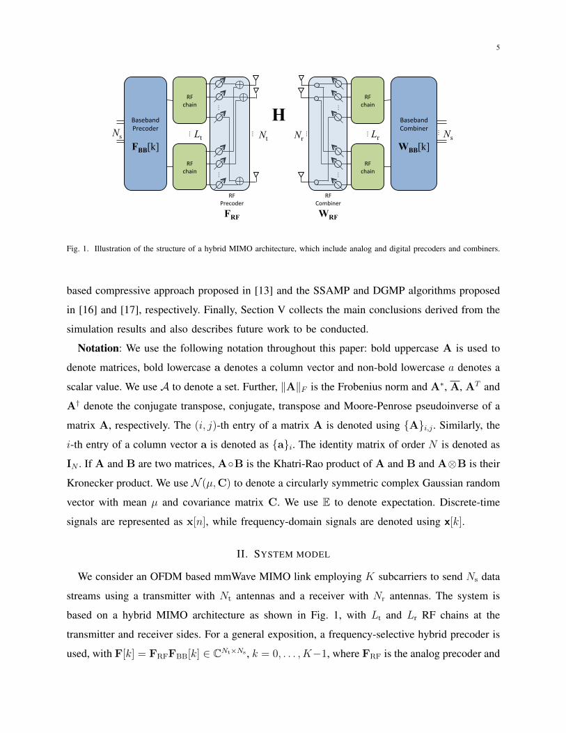
Fig. 1. Illustration of the structure of a hybrid MIMO architecture, which include analog and digital precoders and combiners.
based compressive approach proposed in [13] and the SSAMP and DGMP algorithms proposed
in [16] and [17], respectively. Finally, Section V collects the main conclusions derived from the
simulation results and also describes future work to be conducted.
Notation: We use the following notation throughout this paper: bold uppercase A is used to
denote matrices, bold lowercase a denotes a column vector and non-bold lowercase a denotes a
scalar value. We use A to denote a set. Further, ‖A‖F is the Frobenius norm and A∗, A, AT and
A† denote the conjugate transpose, conjugate, transpose and Moore-Penrose pseudoinverse of a
matrix A, respectively. The (i, j)-th entry of a matrix A is denoted using Ai,j . Similarly, the
i-th entry of a column vector a is denoted as ai. The identity matrix of order N is denoted as
IN . If A and B are two matrices, AB is the Khatri-Rao product of A and B and A⊗B is their
Kronecker product. We use N (µ,C) to denote a circularly symmetric complex Gaussian random
vector with mean µ and covariance matrix C. We use E to denote expectation. Discrete-time
signals are represented as x[n], while frequency-domain signals are denoted using x[k].
II. SYSTEM MODEL
We consider an OFDM based mmWave MIMO link employing K subcarriers to send Ns data
streams using a transmitter with Nt antennas and a receiver with Nr antennas. The system is
based on a hybrid MIMO architecture as shown in Fig. 1, with Lt and Lr RF chains at the
transmitter and receiver sides. For a general exposition, a frequency-selective hybrid precoder is
used, with F[k] = FRFFBB[k] ∈ CNt×Ns , k = 0, . . . , K−1, where FRF is the analog precoder and

6
FBB[k] the digital one. Note that the analog precoder is frequency-flat, while the digital precoder
is different for every subcarrier. The RF precoder and combiner are implemented using a fully
connected network of phase shifters, as described in [12]. The symbol blocks are transformed
into the time domain using Lr parallel K-point IFFTs. As in [14], [20], we consider Zero-
Padding (ZP) to both suppress Inter Symbol Interference (ISI) and account for the RF circuitry
reconfiguration time. The discrete-time complex baseband signal at subcarrier k can be written
as
x[k] = FRFFBB[k]s[k], (1)
where the transmitted symbol sequence at subcarrier k of size Ns × 1 is denoted as s[k].
The MIMO channel between the transmitter and the receiver is assumed to be frequency-
selective, having a delay tap length Nc in the time domain. The d-th delay tap of the channel
is represented by a Nr × Nt matrix denoted as Hd, d = 0, 1, ..., Nc − 1, which, assuming a
geometric channel model [18], can be written as
Hd =
√NtNr
LρL
L∑`=1
α`prc(dTs − τ`)aR(φ`)a∗T(θ`), (2)
where ρL denotes the path loss between the transmitter and the receiver, L denotes the number
of paths, prc(τ) is a filter that includes the effects of pulse-shaping and other lowpass filtering
evaluated at τ , α` ∈ C is the complex gain of the `th path, τ` ∈ R is the delay of the `th
path, φ` ∈ [0, 2π) and θ` ∈ [0, 2π) are the angles-of-arrival and departure (AoA/AoD), of the
`th path, and aR(φ`) ∈ CNr×1 and aT(θ`) ∈ CNt×1 are the array steering vectors for the receive
and transmit antennas. Each one of these matrices can be written in a more compact way as
Hd = AR∆dA∗T, (3)
where ∆d ∈ CL×L is diagonal with non-zero complex entries, and AR ∈ CNr×L and AT ∈ CNt×L
contain the receive and transmit array steering vectors aR(φ`) and aT(θ`), respectively. The
channel Hd can be approximated using the extended virtual channel model defined in [2] as
Hd ≈ AR∆vdA∗T, (4)
where ∆vd ∈ CGr×Gt is a sparse matrix which contains the path gains of the quantized spatial
frequencies in the non-zero elements. The dictionary matrices AT and AR contain the transmitter
and receiver array response vectors evaluated on a grid of size Gr for the AoA and a grid of size

7
Gt for the AoD. Due to the few scattering clusters in mmWave channels, the sparse assumption
for ∆vd ∈ CGr×Gt is commonly accepted.
Finally, the channel at subcarrier k can be written in terms of the different delay taps as
H[k] =Nc−1∑d=0
Hde−j 2πk
Kd. (5)
It is also useful to write this matrix in terms of the sparse matrices ∆vd and the dictionaries
H[k] ≈ AR
(Nc−1∑d=0
∆vde−j 2πk
Kd
)A∗T = AR∆[k]A∗T (6)
to help expose the sparse structure later.
Assuming that the receiver applies a hybrid combiner W[k] = WRFWBB[k] ∈ CNr×Ns , the
received signal at subcarrier k can be written as
y[k] = W∗BB[k]W∗
RFH[k]FRFFBB[k]s[k]
+W∗BB[k]W∗
RFn[k],(7)
where n[k] ∼ N (0, σ2I) is the circularly symmetric complex Gaussian distributed additive noise
vector. The receive signal model in (7) corresponds to the data transmission phase. As we will
see in Section III, during the channel acquisition phase, we will consider analog-only training
precoders and combiners to reduce complexity.
III. COMPRESSIVE CHANNEL ESTIMATION IN THE FREQUENCY DOMAIN
In this section, we formulate a compressed sensing problem to estimate the vectorized sparse
channel vector in the frequency domain. We also propose two algorithms to solve this problem
that leverage the common support between the channel matrices for every subcarrier, providing
different trade-offs complexity-performance. The first algorithm leverages the common support
between the K different subchannels providing a very good performance, while the second one
only exploits information from a reduced number of subcarriers, thereby keeping computational
complexity at a lower level.
A. Problem formulation
We assume that Lt RF chains are used at the transmitter. During the training phase, for the
m-th frame we use a training precoder F(m)tr and a training combining matrix W
(m)tr . This means

8
that during the training phase, only analog precoders and combiners are considered to keep the
complexity of the sparse recovery algorithm low. We assume that the transmitted symbols satisfy
Es(m)[k]s(m)∗[k] = PNs
INs , with P the total transmitted power and Ns = Lt. Furthermore, each
entry in F(m)tr , W
(m)tr is normalized to have squared-modulus N−1t and N−1r , respectively. Then,
the received samples in the frequency domain for the m-th training frame can be written as
y(m)[k] = W(m)tr∗H[k]F
(m)tr s(m)[k] + n(m)
c [k], (8)
where H[k] ∈ CNr×Nt is the frequency-domain MIMO channel response at the k-th subcarrier
and n(m)c [k] ∈ CLr×1, n(m)
c [k] = W(m)tr∗n(m)[k], is the frequency-domain combined noise vector
received at the k-th subcarrier. The average received SNR per transmitted symbol is given by
SNR = Pρ`σ2 . We assume that the channel coherence time is larger than the frame duration and
that the same channel can be considered for several consecutive frames.
Using the result vecAXC = (CT ⊗A) vecX, the vectorized received signal is
vecy(m)[k] = (s(m)T [k]F(m)tr
T⊗W
(m)tr∗) vecH[k]+ n(m)
c [k]. (9)
Taking into account the expression in (6), the vectorized channel matrix can be written as
vecH[k] = ( ¯AT⊗ AR) vec∆[k]. Therefore, if we define the measurement matrix Φ(m)[k] ∈
CLr×NtNr as
Φ(m)[k] = (s(m)T [k]F(m)tr
T⊗W
(m)tr∗) (10)
and the dictionary Ψ ∈ CNtNr×GtGr as
Ψ = ( ¯AT ⊗ AR), (11)
(9) can be rewritten as
vecy(m)[k] = Φ(m)[k]Ψhv[k] + n(m)c [k], (12)
where hv[k] = vec∆[k] ∈ CGrGt×1 is the sparse vector containing the complex channel gains.
To have enough measurements and accurately reconstruct the sparse vector hv[k], it is necessary
to use several training frames, especially in the very-low SNR regime. If the transmitter and
receiver communicate during M training steps using different pseudorandomly built precoders
9
and combiners, (12) can be extended toy(1)[k]
y(2)[k]...
y(M)[k]
︸ ︷︷ ︸
y[k]
=
Φ(1)[k]
Φ(2)[k]...
Φ(M)[k]
︸ ︷︷ ︸
Φ[k]
Ψhv[k] +
n(1)
c [k]
n(2)c [k]...
n(M)c [k]
︸ ︷︷ ︸
nc[k]
. (13)
Finally, the vector hv[k] can be found by solving the sparse reconstruction problem
min ‖hv[k]‖1 subject to ‖y[k]−Φ[k]Ψhv[k]‖22 < ε, (14)
where ε is a tunable parameter defining the maximum error between the measurement and the
received signal assuming the reconstructed channel between the transmitter and the receiver.
Since the sparsity (number of channel paths) is usually unknown, this parameter can be set to
the noise variance [13].
There are a great variety of algorithms to solve (14). We could use, for example, Orthogonal
Matching Pursuit (OMP) to find the sparsest approximation of the vectors containing the channel
gains. Since the vector hv[k] depends on the frequency bin, it would be necessary to run the
algorithm as many times as the number of subcarriers at which the MIMO channel response
is to be estimated. In the next subsections we consider an additional assumption to solve this
problem, which avoids the need to run K OMP algorithms in parallel as proposed in [14].
The formulation in (8)-(14) is provided as a general framework to leverage the sparse structure
of the frequency-selective mmWave channel. This formulation, however, leads to subcarrier-
dependent measurement matrices, resulting in high computational complexity for channel esti-
mation. Using more than a single RF chain at the transmitter offers more degrees of freedom
to design the measurement matrices and, consequently, obtain better estimation performance.
Nonetheless, exploiting these degrees of freedom results in additional computational complexity
with regard to the case of using a single RF chain at the transmitter. Furthermore, the difference
in performance between using Lt = 1 and Lt > 1 was observed to be less than 0.5 dB when
solving the problem with the algorithm proposed in this section, which comes from the fact that a
reasonable number of RF chains must be used at a given transceiver to keep power consumption
low. For this reason, our focus is on designing algorithms exhibiting reasonable performance
and low computational complexity.
10
For this reason, we consider the special case of Lt = 1 to present our algorithms with reduced
complexity. With this choice, the frequency-selective transmitted symbols are scalar and its effect
can be easily inverted at the receiver (i.e., by multiplying by (s(m)[k])−1 or multiplying by s(m)[k]
if the transmitted symbols belong to a QPSK constellation with energy-normalized symbols).
As shown in Section IV, the use of a single frequency-flat measurement matrix is enough to
asymptotically attain the CRLB with on-grid channel parameters. Therefore, a single RF chain
and analog-only precoders are used during training, thereby managing a reasonable trade-off
between performance and computational complexity. Nonetheless, the algorithms we propose
in the next subsections can be easily extended to work with subcarrier-dependent measurement
matrices.
By compensating for s(m)[k], for a given training step m, the measurement matrix Φ(m)[k]
reduces to Φ(m) = f(m)tr
T⊗W
(m)∗tr . At this point, it is important to highlight that: 1) Analog-only
training precoders and combiners are used to keep computational complexity low, and 2) A single
data stream is transmitted to guarantee that the same measurement matrix is enough to estimate
the different frequency-domain subchannels. In fact, these choices enable both online and offline
complexity reduction when the noise statistics are used to estimate the MIMO channel at the
different subcarriers.
The matrices ∆[k] exhibit an interesting property that can be exploited when solving the
compressed channel estimation problems defined in (14). Let us define the GtGr × 1 vectorized
virtual channel matrix for a given delay tap as
hvd , vec∆v
d. (15)
Let us denote the supports of the virtual channel matrices ∆vd as T0, T1, . . . , TNc−1, d = 0, . . . , Nc−
1. Then, since hv[k] = vec∆[k], with ∆[k] =∑Nc−1
d=0 ∆vde−j 2πk
Nd, k = 0, . . . , K− 1, it is clear
that
supphv[k] =Nc−1⋃d=0
supphvd k = 0, . . . , K − 1, (16)
where the union of the supports of the time-domain virtual channel matrices comes from the
additive nature of the Fourier transform. The sparse assumption on the vectorized channel matrix
for a given delay tap hvd is commonly accepted, since in mmWave channels L << GrGt. The
vectorized channel matrix hv[k] will have, in the worst case, NcL non-zero coefficients. Typical
values for Nc in mmWave channels are usually lower than 64 symbols (for example IEEE
11
802.11ad has been designed to work robustly for a maximum of 64 delay taps in the channel),
while the number of measured paths usually satisfies L < 30 for outdoor and indoor scenarios
[21]. From these values, using dictionaries of size Gr ≥ 64 Gt ≥ 64, allows us to assume a
spatially sparse structure for hv[k] as well. Furthermore, this sparse structure is the same for all
k, since from (6), AR and AT do not depend on k, which means that the AoAs and AoDs do
not change with frequency in the transmission bandwidth.
B. Simultaneous weighted estimation exploiting common support between subcarriers (SW-OMP)
To develop a channel estimation algorithm that leverages the sparse nature and the common
support property for all hv[k], we propose to modify the S-OMP algorithm proposed in [22].
For a given iteration, this algorithm aims at finding a new index of the support such that its
likelihood is larger than if the signals for the different subbands were individually processed. In
this way, the K different signals contribute to decide which is the most likely index belonging
to the support in a cooperative fashion. The S-OMP algorithm in [22] computes the gains of
the sparse vector using a LS approach once the support is obtained, assuming that the noise
covariance matrix is the identity matrix IMLr . In this paper, we propose two modifications of
the S-OMP for the estimation of the support and the channel gains. The first one accounts for
the correlated nature of the noise at the output of the RF combiner, and leads to a more precise
estimation of the support in this particular application. The second one consists of a different
approach to compute the channel gains. In particular, we develop the minimum variance unbiased
estimator for the channel gains, which is shown to be a weighted LS estimator. We show that
this estimator attains the CRLB.
1) Support computation with correlated noise: Before explicit estimation of the channel gains,
it is necessary to compute the atom, i.e., vector in the measurement matrix, which yields the
largest sum-projection onto the received signals, provided that the support of the different sparse
vectors is the same. The S-OMP algorithm is based on the assumption that the perturbation (noise)
covariance matrix is diagonal, such that no correlation between the different noise components
is present. The projection vector c[k] ∈ CMLr is defined as
c[k] = Υ∗y[k], (17)
in which Υ ∈ CMLr×GtGr , Υ = ΦΨ is the measurement matrix and y[k] ∈ CMLr×1 is the received
signal for a given k, k = 0, . . . , K − 1. If there is correlation between noise components, the

12
atom estimated from the projection in (17) is not likely to be the actual one. To introduce the
appropriate correction in the projection, the specific form the noise covariance matrix takes needs
to be used. It is important to highlight that depending on the design of the combiners for each
of the M training steps, the noise statistics will be different. Specifically, the noise covariance
matrix contains the (complex) inner product between the different hybrid combiners, for each
training step m, m = 1, . . . ,M . Let us consider two arbitrary (hybrid) combiners W(m)tr
(i),
W(m)tr
(j)∈ CNr×Lr for two arbitrary training steps i,j and a given subcarrier k. Therefore, if the
combined noise at a given training step i and subcarrier k is denoted as n(i)c [k] = W
(m)tr
(i)∗n(i)[k],
with n(i)[k] ∼ N (0, σ2ILr), the noise cross-covariance matrix is given by
En(i)c [k]n(j)∗
c [k] = EW(m)tr
(i)∗n(i)[k]n(j)∗[k]W
(m)tr
(j)
= W(m)tr
(i)∗En(i)[k]n(j)∗[k]W(m)
tr(j)
= W(m)tr
(i)∗σ2δ[i− j]W(m)
tr(j), (18)
such that it is the same for all subcarriers during training. It can be written as a block diagonal
matrix C ∈ CMLr×MLr whose i-th diagonal block is the Gram matrix of the (hybrid) combiner
W(i), that is, C = σ2Cw, where
Cw = blkdiagW(m)tr
(1)∗W
(m)tr
(1),W
(m)tr
(2)∗W
(m)tr
(2), . . . ,W
(m)tr
(M)∗W
(m)tr
(M). (19)
Now, we can resort to the Cholesky decomposition of Cw
Cw = D∗wDw, (20)
with Dw ∈ CMLr×MLr an upper triangular matrix. The subscript in Cw and Dw indicates that
these matrices only depend on the combiners W(m)tr used during M consecutive training frames.
Therefore, the projection step is performed as
c[k] = Υ∗wy[k], (21)
where Υw ∈ CMLr×GtGr is the whitened measurement matrix given by Υw = D−1w Υ. In this way,
the resulting projection simultaneously whitens the spatial noise components and estimates the
projection of the received signal onto the subspace spanned by the columns in the measurement
matrix.
13
2) Computation of the channel gains: If the vectorized channel matrix for a given subcarrier
k, k = 0, 1, . . . , K − 1, is given by vecH[k] = (AT AR)ξ[k], with ξ[k] the L × 1 vector
of channel gains, then the received signal y[k] is distributed according to N (ΦΨξ[k],C). Once
the different AoAs/AoDs are found, the signal model for the k-th subcarrier can be written as
y[k] = Υ:,T ξ[k] + nc[k], (22)
where nc[k] ∈ CMLr×1 is the residual noise in our linear model after estimating the channel
support. If the estimation of the support is accurate, nc[k] will be close to the post-combining
noise vector nc[k]. The L × 1 vector ξ[k] is the vector of channel gains to be estimated after
sparse recovery, where L = |T | is the estimate of the sparsity level. The matrix Υ:,T ∈ CMLr×L
is defined as
Υ:,T =[ΦΨ
]:,T . (23)
It is important to remark that the support estimated by the proposed algorithm may be different
from the actual channel support. Provided that, in general, T can be different from the actual
support, the vector ξ[k] ∈ CL×1 containing the complex channel gains can be also different from
the vector containing the true channel gains. Since the model in (22) is linear on the parameter
vector ξ[k], there is a Minimum Variance Unbiased (MVU) Estimator that happens to be the
Best Linear Unbiased Estimator (BLUE) as well [23].
The mathematical equation in (22) is usually referred to as the General Linear Model (GLM),
for which the solution of ξ[k] for real parameters is provided in [23]. The extension for a complex
vector of parameters is straightforward and given by
ˆξ[k] = (Υ∗:,T C−1Υ:,T )
−1Υ∗:,T C−1y[k]. (24)
Therefore, ˆξ[k] is the MVU estimator for our parameter vector ξ[k], k = 0, . . . , K − 1. Hence,
it is unbiased and attains the CRLB is the support is estimated correctly. It is interesting to
note that this corresponds to a Weighted Least-Squares (WLS) estimator, with the corresponding
weights given by the inverse covariance matrix of the noise. We are interested in finding the
CRLB for the estimation of the channel matrices at each subcarrier assuming perfect sparse
reconstruction. To that end, taking into account only the non-zero entries in hv[k], the Fisher
Information Matrix (FIM) is derived from the GLM in (13) as
I(ξ[k]) = Υ∗:,T C−1Υ:,T . (25)
14
Note that the previous expression gives the FIM for the vector ξ[k], which contains the actual
channel gains. Accordingly, the overall variance of the estimator for the vector of channel gains
is given by the sum of the individual CRLBs for each of the complex gains. Therefore, if we
denote the overall variance of the estimator for ξ[k] as γ(ξ[k]), k = 0, 1, . . . , K − 1, then
CRLB(ξ[k]) = I−1(ξ[k]) (26)
and
γ(ξ[k]) = traceCRLB(ξ[k]). (27)
The last equation only takes into account the channel gains for each path in the extended virtual
channel representation. Our interest, however, is to compare the channel estimation performance
at the antenna level. To that end, the frequency-domain channel matrix can be vectorized as
(subcarrier-wise)
vecH[k] = (AT AR)ξ[k], (28)
where AT ∈ CNt×L, AR ∈ CNr×L are the array response matrices evaluated on the AoAs/AoD.
Notice that the decomposition in (28) is expressed with equality, which follows from the assump-
tion that the estimation of the support is perfect and only the channel gains are to be estimated.
The assumption on the perfect estimation of the support comes from the fact that the channel
vectors hv[k] are assumed to be sparse and the AoA/AoD are estimated perfectly. Since the
Fisher Information requires that the mean of the received signal is continuous and differentiable
on the parameters to estimate, it cannot be applied to the estimation of the angular parameters.
Owing to our lacking space, the solution to the problem of finding the CRLB in a more general
case accounting for continuous AoA and AoD is left for future work.
The overall minimum variance for an unbiased estimator of the NtNr entries in H[k] is
given by the sum of the variances for each element H[k]i,j, i = 1, . . . , Nr, j = 1, . . . , Nt.
Mathematically, following the same notation as with γ(ξ[k]), we will denote the overall variance
of the estimator for H[k] as γ(vecH[k]), for a given subcarrier k. Then, γ(vecH[k]) is
derived as
γ(vecH[k]) = trace
∂ vecH[k]
∂ξ[k]CRLB(ξ[k])
∂ vecH∗[k]∂ξ[k]
= trace
(AT AR)CRLB(ξ[k])(AT AR)∗
. (29)

15
An important feature of this estimator is that the difference in performance given by the LS
and the WLS estimators is more accentuated as the number of RF chains grows (if and only if
the hybrid combiner is not built from orthonormal vectors). Furthermore, this estimator works
even though the noise variance is unknown. This is because the noise covariance matrix C
can be written as C = σ2Cw, where Cw models the coupling between the different combining
vectors. Since the combining vectors are known at the receiver, this matrix Cw is known as well.
Therefore, we can write our estimator for the vector containing the channel gains, ˆξ[k] ∈ CL×1
asˆξ[k] = (Υ∗:,T C
−1w Υ:,T )
−1Υ∗:,T C−1w y[k]. (30)
When the noise variance is unknown, it follows from the Slepian-Bangs formula that the CRLB
for the vector ξ[k] does not change, since the noise mean does not depend on the variance σ2.
Thus, the elements in the FIM modeling the coupling between the noise variance and the channel
gains are zero. Therefore, the estimator of ξ[k] is efficient. In fact, it is also the ML estimator for
this complex parameter vector, since it can be seen to maximize the Log-Likelihood Function
(LLF) of the received signal. Nonetheless, there is no efficient estimator for both ξ[k] and σ2,
since the MVUE of σ2 depends on the true value for ξ[k]. Despite this, the MLE for σ2 can
still be found by setting the partial derivative of the LLF to zero. If we use the identities
∂ ln detC∂σ2
= trace
C−1
∂C
∂σ2
(31)
and
∂(y[k]−Υ:,T ˆξ[k])∗C−1(y[k]−Υ:,T
ˆξ[k])
∂σ2= −(y[k]−Υ:,T
ˆξ[k])∗C−1×
∂C
∂σ2C−1 × (y[k]−Υ:,T
ˆξ[k]),
(32)
it is possible to find that
σ2 =1
MLr(y[k]−Υˆξ[k])∗C−1w (y[k]−Υˆξ[k]). (33)
Finally, we can consider the information coming from all the subcarriers to enhance the
estimation of the noise variance. For the different subcarriers, we have the model
σ2[k] = σ2 + ν[k], k = 0, . . . , K − 1, (34)
where ν[k] models the estimation error for the variance in the k-th subcarrier. We known that,
in high SNR regime, the ML estimator is Gaussian distributed. Therefore, we have a set of K

16
linear models for the estimation of the variance. Since the model is linear on the parameter σ2,
we find that the ML of the variance is also the BLUE estimator, given by
σ2ML =
1
K1Tσ, (35)
where σ ∈ RK×1 is defined as σ = [σ2[0], σ2[1], . . . , σ2[K − 1]]T and 1 is the K × 1 column
vector containing a 1 in each position.
Algorithm 1 Simultaneous Weighted Orthogonal Matching Pursuit (SW-OMP)1: procedure SW-OMP(z[k],Φ,Ψ,ε)
2: Compute the equivalent observation matrix
3: Υ = ΦΨ
4: Initialize the residual vectors to the input signal vectors and support estimate
5: r[k] = y[k], k = 0, . . . , K − 1, T = ∅
6: while MSE > ε do7:
8: Distributed Projection
9: c[k] = Υ∗D−∗w r[k], k = 0, . . . , K − 1
10: Find the maximum projection along the different spaces
11: p? = arg maxp
∑K−1k=0 |c[k]p|
12: Update the current guess of the common support
13: T = T ∪ p?14:
15: Project the input signal onto the subspace given by the support using WLS
16: xT [k] = (Υ∗:,T C−1w Υ:,T )
−1Υ∗:,T C−1w y[k], k = 0, . . . , K − 1
17: T ∪ T = 1, 2, . . . , GtGr , T ∩ T = ∅18:
19: Update residual
20: r[k] = y[k]−Υ:,T ˆξ[k] , where ˆξ[k] = xT [k], k = 0, . . . , K − 121:
22: Compute the current MSE
23: MSE = 1KMLr
∑K−1k=0 r∗[k]C−1w r[k]24:
25: end while
26: end procedure
The derived estimator for the channel gains ξ[k] can be used in the S-OMP algorithm. In
fact, the larger the number of subcarriers, the smaller the estimation variance the ML estimator
17
can achieve. Thereby, if the number of averaging subcarriers K is large enough, the lack of
knowledge of the sparsity level is not so critical because of two reasons: 1) the computation
of the support is more precise due to noise averaging during the projection process, and 2)
if the support is estimated correctly, a particular estimate of σ2 will be very close to the true
noise variance, such that the chosen halting criterion is optimal from the Maximum Likelihood
perspective. It should be clear that the higher the covariance between adjacent noise components,
the larger the performance gap between the S-OMP and the SW-OMP algorithm will be, which
actually depends on the ratio between Nr (Nt) and Lr (Lt).
The modification of the S-OMP algorithm to include the MVU estimator for the channel
gains, as well as the whitening matrix to estimate the support is provided in Algorithm 1. Notice
that the proposed algorithm performs both noise whitening and channel estimation, such that
interferences due to noise correlation are mitigated.
C. Subcarrier Selection Simultaneous Weighted-OMP + Thresholding
Despite the use of a single, subcarrier-independent measurement matrix Υ to estimate the
frequency-domain channels, the algorithm presented in the previous section exhibits high com-
putational complexity. The SW-OMP algorithm considers the distributed projection coming
from every subcarrier; however, a trade-off between performance and computational complexity
can be achieved if a small number of subcarriers Kp << K is used, instead. The problem
amounts as to how to choose those subcarriers, since no quality measure is available beforehand.
The ideal situation would require knowledge of the Signal-to-Noise Ratio (SNR), which is
unknown so far. Nonetheless, we have access to different frequency-domain received vectors
y[k], k = 0, 1, . . . , K− 1. Therefore, the quality measure to be used could be the l2-norm of the
different vectors. Thereby, the Kp subcarriers having largest l2-norm can be used to derive an
estimate of the support of the already defined sparse channel vectors hv[k], k = 0, . . . , K − 1.
The main problem concerning Matching Pursuit (MP) algorithms comes from the lack of
knowledge of the channel sparsity L. For this reason, there is usually an iteration at which L
paths have been detected but the estimate of the average residual energy is a little larger than
the noise variance itself. This makes the algorithm find additional paths which are not actually
contained in the MIMO channel. These paths usually have low power, and a pruning procedure
is needed to filter out these undesired components.

18
Algorithm 2 Subcarrier Selection Simultaneous Weighted Orthogonal Matching Pursuit +
Thresholding (SS-SW-OMP+Th)1: procedure SS-SW-OMP(y[k],Φ,Ψ,KP ,β ,ε)
2: Initialize counter, set of subcarriers and residual vectors
3: i = 0, K = ∅, r[k] = y[k], k = 0, . . . , K − 1
4: Find the Kp strongest subcarriers
5: while i ≤ Kp do
6: K = K ∪ arg maxk 6∈K
‖y[k]‖227: i = i+ 1
8: end while
9: Compute the equivalent observation matrix
10: Υ = ΦΨ
11: while MSE > ε do
12: Distributed Projection
13: c[k] = Υ∗D−∗w r[k], k ∈ K
14: Find the maximum projection along the different spaces
15: p? = arg maxp
∑k∈K |c[k]p|
16: Update the current guess of the common support
17: T = T ∪ p?
18: Project the input signal onto the subspace given by the support using WLS
19: xT [k] = (Υ∗:,T C−1w Υ:,T )
−1Υ∗:,T C−1w y[k], k = 0, . . . , K − 1
20: xT = 0, where T ∪ T = 1, 2, . . . , GtGr , T ∩ T = ∅
21: Update residual
22: r[k] = y[k]−Υ:,T ˆξ[k] , where ˆξ[k] = xT [k], k = 0, . . . , K − 1
23: Compute the current MSE
24: MSE = 1KMLr
∑K−1k=0 r∗[k]C−1w r[k]
25: end while
26: Thresholding based on maximum average power
27: P ? = max`
1K
∑K−1k=0 |ξ[k]`|2, pav,i = 1
K
∑K−1k=0 |ξ[k]i|2, i = 1, . . . , L
28: TTh =⋃i / pav,i ≥ βP ?, i ∈ T
29: ξ[k] = ξ[k]TTh, k = 0, . . . , K − 1
30: end procedure
19
A reasonable way to prune the undesired paths is to remove those components whose power
falls below a given threshold, which can be related to the average power of the component
in the estimated sparse vectors having maximum average power. Let us denote this power by
P ?. Then, the threshold can be defined as η = βP ?, β ∈ (0, 1). The value P ? is taken as
P ? = max`
1K
∑K−1k=0 |ξ[k]`|2. To keep the common sparsity property we must ensure that
the channel support after thresholding remains invariant. For this purpose, we define a signal
pav ∈ CL×1 whose i-th component is given by pav,i = 1K
∑K−1k=0 |ξ[k]i|2, i = 1, . . . , L, such
that pav measures the average power along the different subbands of each spatial component in the
quantized angle grid. The final support after thresholding TTh is defined as TTh =⋃Li=1 i / pav,i ≥
βP ?. Therefore, the components in ξ[k] indexed by TTh are the final channel gains estimates for
each subcarrier. The modification of the proposed SW-OMP algorithm to reduce computational
complexity and implement this pruning procedure is provided in Algorithm 2.
IV. RESULTS
This section includes the main empirical results obtained with the two proposed algorithms,
SW-OMP and SS-SW-OMP + Thresholding, and comparisons with other the frequency-domain
channel estimation algorithms including SSAMP [16] and DGMP [17]. To obtain these results,
we perform Monte Carlo simulations averaged over many trials to evaluate the normalized mean
squared error (NMSE) and the ergodic rate as a function of SNR and number of training frames
M . We also provide calculations of the computational complexity for the proposed algorithms
in Table I and prior work in Table II.
The typical parameters for our system configuration are summarized as follows. Both the
transmitter and the receiver are assumed to use Uniform Linear Arrays (ULAs) with half-
wavelength separation. Such a ULA has steering vectors obeying the expressions aT(θ`)n =√1Ntejnπ cos (θ`), n = 0, . . . , Nt − 1 and aR(φ`)m =
√1Nrejmπ cos (φ`), m = 0, . . . , Nr − 1.
We take Nt = Nr = 32 and Gt = Gr = 64. The phase-shifters used in both the transmitter and
the receiver are assumed to have NQ quantization bits, so that the entries of the training vectors
f(m)tr , w
(m)tr , m = 1, 2, . . . ,M are drawn from a set A =
0, 2π
2NQ, . . . , 2π(2
NQ−1)2NQ
. The number of
RF chains is set to Lt = 1 at the transmitter and Lr = 4 at the receiver. The number of OFDM
subcarriers is set to K = 16.
We generate channels according to (2) with the following parameters:

20
• The L = 4 channel paths are assumed to be independent and identically distributed, with
delay τ` chosen uniformly from [0, (Nc − 1)Ts], with Ts = 11760
s, as in the IEEE 802.11ad
wireless standard.
• The AoAs/AoDs are assumed to be uniformly distributed in [0, π).
• The gains of each path are zero-mean complex Gaussian distributed such that Ek‖H[k]‖2F =
NrNtρL
.
• The band-limiting filter prc(t) is assumed to be a raised-cosine filter with roll-off factor of
0.8.
• The number of delay taps of the channel is set to Nc = 4 symbols.
The simulations we perform consider channel realizations in which the AoA/AoD are off-grid,
i.e. do not correspond to the angles used to build the dictionary, and also the on-grid case, to
analyze the loss due to the model mismatch.
A. NMSE Comparison
One performance metric is the Normalized Mean Squared Error (NMSE) of a channel estimate
H[k] for a given realization, defined as
NMSE =
∑K−1k=0 ‖H[k]−H[k]‖2F∑K−1
k=0 ‖H[k]‖2F. (36)
The NMSE will be our baseline metric to compute the performance of the different estimators,
and will be averaged over many channel realizations. The normalized CRLB (NCRLB) is also
provided to compare the average performance of each algorithm with the lowest achievable
NMSE, and will also be averaged over many channel realizations
NCRLB =
∑K−1k=0 CRLB(vecH[k])∑K−1
k=0 ‖H[k]‖2F. (37)
We compare the average NMSE versus SNR obtained for the different channel estimation
algorithms in Fig. 2 for a practical SNR range of −15 dB to 10 dB, on-grid AoA/AoDs, and two
different values for the number of training frames. SW-OMP performs the best, achieving NMSE
values very close to the NCRLB. SS-SW-OMP+Th performs similarly to SW-OMP, although
there is some performance loss due to the fact that SS-SW-OMP+Th does not employ every
subcarrier to estimate the common support of the sparse channel vectors. In SS-SW-OMP+Th,
the number of selected subcarriers for the estimation of the support was set to Kp = 4 for
21
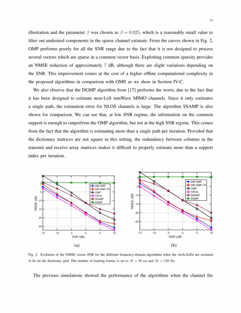
illustration and the parameter β was chosen as β = 0.025, which is a reasonably small value to
filter out undesired components in the sparse channel estimate. From the curves shown in Fig. 2,
OMP performs poorly for all the SNR range due to the fact that it is not designed to process
several vectors which are sparse in a common vector basis. Exploiting common sparsity provides
an NMSE reduction of approximately 7 dB, although there are slight variations depending on
the SNR. This improvement comes at the cost of a higher offline computational complexity in
the proposed algorithms in comparison with OMP, as we show in Section IV-C.
We also observe that the DGMP algorithm from [17] performs the worst, due to the fact that
it has been designed to estimate near-LoS mmWave MIMO channels. Since it only estimates
a single path, the estimation error for NLOS channels is large. The algorithm SSAMP is also
shown for comparison. We can see that, at low SNR regime, the information on the common
support is enough to outperform the OMP algorithm, but not at the high SNR regime. This comes
from the fact that the algorithm is estimating more than a single path per iteration. Provided that
the dictionary matrices are not square in this setting, the redundancy between columns in the
transmit and receive array matrices makes it difficult to properly estimate more than a support
index per iteration.
-15 -10 -5 0 5 10
SNR (dB)
-25
-20
-15
-10
-5
0
NM
SE
(d
B)
SW-OMP
SW-OMP+Th
OMP
CRLB
SSAMP
DGMP
-15 -10 -5 0 5 10
SNR (dB)
-25
-20
-15
-10
-5
0
NM
SE
(d
B)
SW-OMP
SW-OMP+Th
OMP
CRLB
SSAMP
DGMP
(a) (b)
Fig. 2. Evolution of the NMSE versus SNR for the different frequency-domain algorithms when the AoA/AoDs are assumed
to lie on the dictionary grid. The number of training frames is set to M = 80 (a) and M = 120 (b).
The previous simulations showed the performance of the algorithms when the channel fits

22
the on-grid model, but it is also important to analyze the performance in a practical scenario,
when the AoA/AoD do not fall within the quantized spatial grid. Fig. 3 shows the performance
of the different algorithms for off-grid angular parameters. It can be observed that when using
Gt = Gr = 64 there is a considerable loss in performance due to the use of a fixed dictionary
to estimate the AoA/AoD. However, the estimation error is below −10 dB for values of SNR
in the order of 0 and beyond. On the other hand, provided that the SNR expected in mmWave
communication systems is in the order of −20 dB up to 0 dB, the large gap between the proposed
algorithms and the NCRLB needs to be reduced. Increasing the size of the dictionary is one of the
possible solutions, as shown by the curves corresponding to Gt = Gr = 128 and Gt = Gr = 256.
-15 -10 -5 0 5 10
SNR (dB)
-25
-20
-15
-10
-5
0
NM
SE
(dB
)
SW-OMP
SW-OMP+Th
OMP
CRLB
Gt = Gr = 64
Gt = Gr = 128
Gt = Gr = 256
-15 -10 -5 0 5 10
SNR (dB)
-25
-20
-15
-10
-5
0N
MS
E (
dB
)
SW-OMP
SW-OMP+Th
OMP
CRLB
Gr = Gt = 64
Gr = Gt = 128
Gr = Gt = 256
(a) (b)
Fig. 3. Evolution of the NMSE versus SNR for the different frequency-domain algorithms. The number of training frames is
set to M = 80 (a) and M = 120 (b). The AoD/AoA are generated from a continuous uniform distribution.
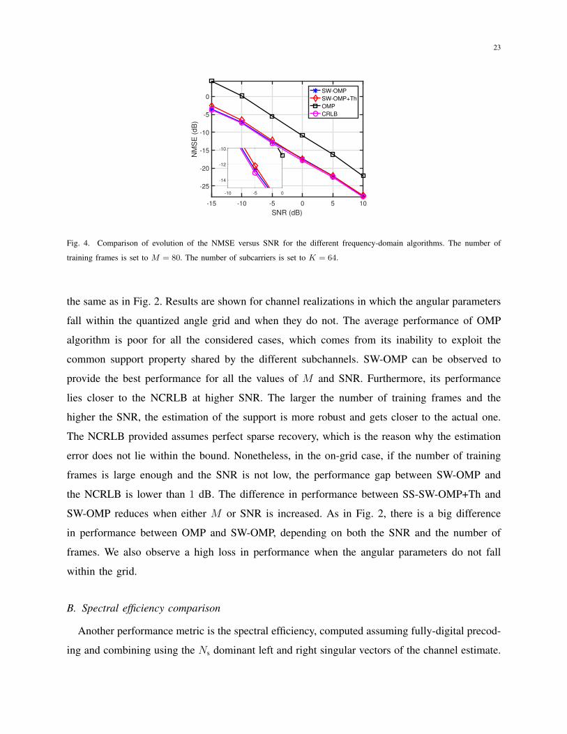
We show in Fig. 4 the performance of the different frequency-domain algorithms when
increasing the number of subcarriers. The parameters for the simulation scenario are the same
as in Fig. 2, however, the number of subcarriers is set to K = 64 in this case. Kp is set
to 32 subcarriers and β = 0.025σ2. Interestingly, both SW-OMP and SS-SW-OMP+Th are
asymptotically efficient since they are both unbiased and attain the NCRLB. A magnified plot
for SNR = −5 dB is also shown to clearly see the performance gap between the different
algorithms and also the NCRLB.
Fig. 5 shows the average NMSE vs number of training frames M . The number of training
frames M is increased from 20 to 100. The remaining parameters in the simulation scenario are
23
-15 -10 -5 0 5 10
SNR (dB)
-25
-20
-15
-10
-5
0
NM
SE
(dB
)
SW-OMP
SW-OMP+Th
OMP
CRLB
-10 -5 0
-14
-12
-10
Fig. 4. Comparison of evolution of the NMSE versus SNR for the different frequency-domain algorithms. The number of
training frames is set to M = 80. The number of subcarriers is set to K = 64.
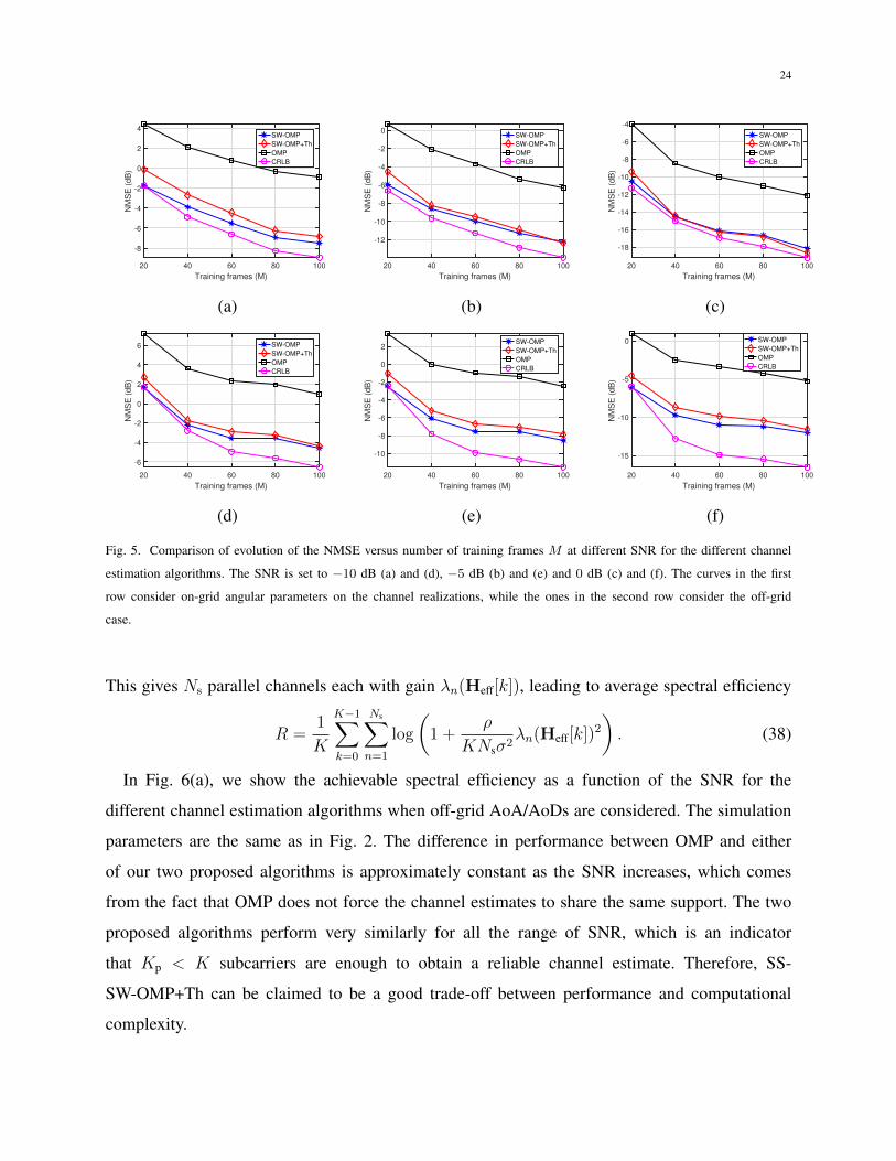
the same as in Fig. 2. Results are shown for channel realizations in which the angular parameters
fall within the quantized angle grid and when they do not. The average performance of OMP
algorithm is poor for all the considered cases, which comes from its inability to exploit the
common support property shared by the different subchannels. SW-OMP can be observed to
provide the best performance for all the values of M and SNR. Furthermore, its performance
lies closer to the NCRLB at higher SNR. The larger the number of training frames and the
higher the SNR, the estimation of the support is more robust and gets closer to the actual one.
The NCRLB provided assumes perfect sparse recovery, which is the reason why the estimation
error does not lie within the bound. Nonetheless, in the on-grid case, if the number of training
frames is large enough and the SNR is not low, the performance gap between SW-OMP and
the NCRLB is lower than 1 dB. The difference in performance between SS-SW-OMP+Th and
SW-OMP reduces when either M or SNR is increased. As in Fig. 2, there is a big difference
in performance between OMP and SW-OMP, depending on both the SNR and the number of
frames. We also observe a high loss in performance when the angular parameters do not fall
within the grid.
B. Spectral efficiency comparison
Another performance metric is the spectral efficiency, computed assuming fully-digital precod-
ing and combining using the Ns dominant left and right singular vectors of the channel estimate.
24
20 40 60 80 100
Training frames (M)
-8
-6
-4
-2
0
2
4N
MS
E (
dB
)SW-OMP
SW-OMP+Th
OMP
CRLB
20 40 60 80 100
Training frames (M)
-12
-10
-8
-6
-4
-2
0
NM
SE
(dB
)
SW-OMP
SW-OMP+Th
OMP
CRLB
20 40 60 80 100
Training frames (M)
-18
-16
-14
-12
-10
-8
-6
-4
NM
SE
(dB
)
SW-OMP
SW-OMP+Th
OMP
CRLB
(a) (b) (c)
20 40 60 80 100
Training frames (M)
-6
-4
-2
0
2
4
6
NM
SE
(dB
)
SW-OMP
SW-OMP+Th
OMP
CRLB
20 40 60 80 100
Training frames (M)
-10
-8
-6
-4
-2
0
2
NM
SE
(dB
)
SW-OMP
SW-OMP+Th
OMP
CRLB
20 40 60 80 100
Training frames (M)
-15
-10
-5
0
NM
SE
(dB
)
SW-OMP
SW-OMP+Th
OMP
CRLB
(d) (e) (f)
Fig. 5. Comparison of evolution of the NMSE versus number of training frames M at different SNR for the different channel
estimation algorithms. The SNR is set to −10 dB (a) and (d), −5 dB (b) and (e) and 0 dB (c) and (f). The curves in the first
row consider on-grid angular parameters on the channel realizations, while the ones in the second row consider the off-grid
case.
This gives Ns parallel channels each with gain λn(Heff[k]), leading to average spectral efficiency
R =1
K
K−1∑k=0
Ns∑n=1
log
(1 +
ρ
KNsσ2λn(Heff[k])2
). (38)
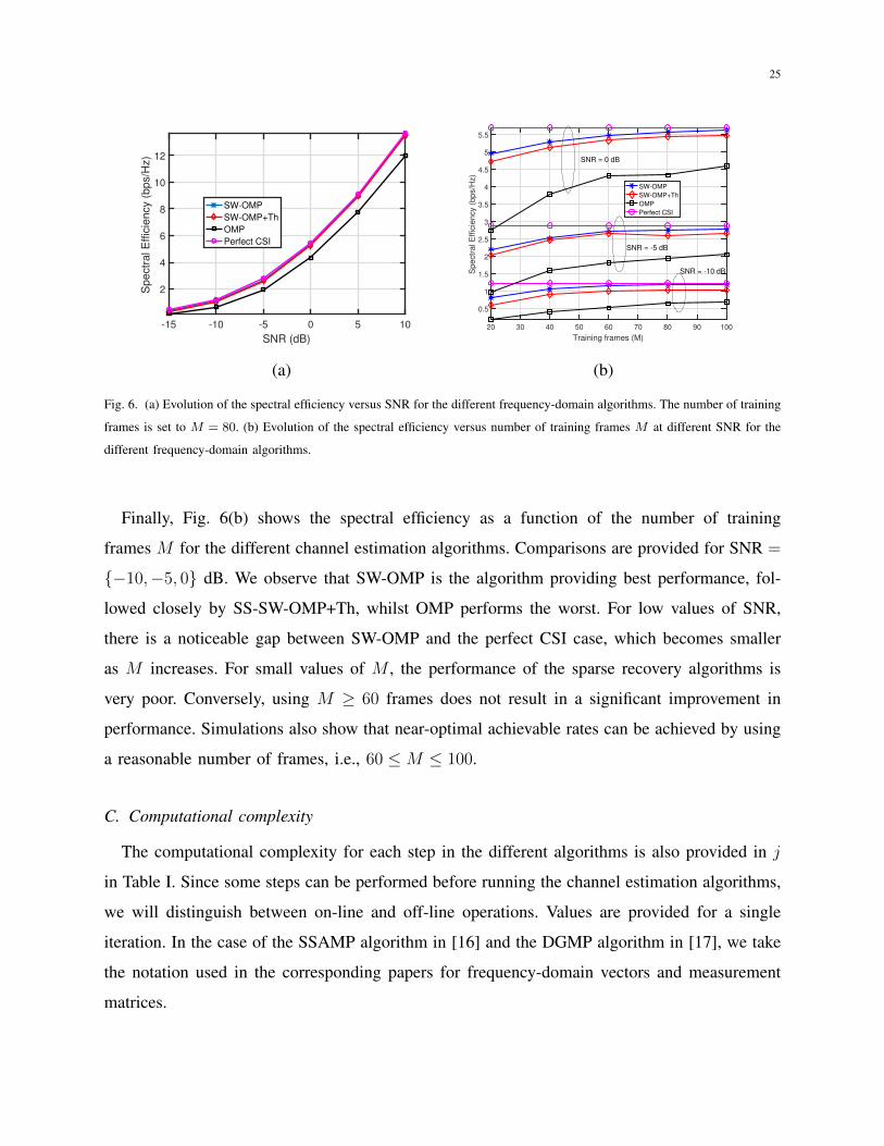
In Fig. 6(a), we show the achievable spectral efficiency as a function of the SNR for the
different channel estimation algorithms when off-grid AoA/AoDs are considered. The simulation
parameters are the same as in Fig. 2. The difference in performance between OMP and either
of our two proposed algorithms is approximately constant as the SNR increases, which comes
from the fact that OMP does not force the channel estimates to share the same support. The two
proposed algorithms perform very similarly for all the range of SNR, which is an indicator
that Kp < K subcarriers are enough to obtain a reliable channel estimate. Therefore, SS-
SW-OMP+Th can be claimed to be a good trade-off between performance and computational
complexity.
25
-15 -10 -5 0 5 10
SNR (dB)
2
4
6
8
10
12S
pectr
al E
ffic
iency (
bps/H
z)
SW-OMP
SW-OMP+Th
OMP
Perfect CSI
20 30 40 50 60 70 80 90 100
Training frames (M)
0.5
1
1.5
2
2.5
3
3.5
4
4.5
5
5.5
Sp
ectr
al E
ffic
ien
cy (
bp
s/H
z)
SW-OMP
SW-OMP+Th
OMP
Perfect CSI
SNR = 0 dB
SNR = -5 dB
SNR = -10 dB
(a) (b)
Fig. 6. (a) Evolution of the spectral efficiency versus SNR for the different frequency-domain algorithms. The number of training
frames is set to M = 80. (b) Evolution of the spectral efficiency versus number of training frames M at different SNR for the
different frequency-domain algorithms.
Finally, Fig. 6(b) shows the spectral efficiency as a function of the number of training
frames M for the different channel estimation algorithms. Comparisons are provided for SNR =
−10,−5, 0 dB. We observe that SW-OMP is the algorithm providing best performance, fol-
lowed closely by SS-SW-OMP+Th, whilst OMP performs the worst. For low values of SNR,
there is a noticeable gap between SW-OMP and the perfect CSI case, which becomes smaller
as M increases. For small values of M , the performance of the sparse recovery algorithms is
very poor. Conversely, using M ≥ 60 frames does not result in a significant improvement in
performance. Simulations also show that near-optimal achievable rates can be achieved by using
a reasonable number of frames, i.e., 60 ≤M ≤ 100.
C. Computational complexity
The computational complexity for each step in the different algorithms is also provided in j
in Table I. Since some steps can be performed before running the channel estimation algorithms,
we will distinguish between on-line and off-line operations. Values are provided for a single
iteration. In the case of the SSAMP algorithm in [16] and the DGMP algorithm in [17], we take
the notation used in the corresponding papers for frequency-domain vectors and measurement
matrices.
26
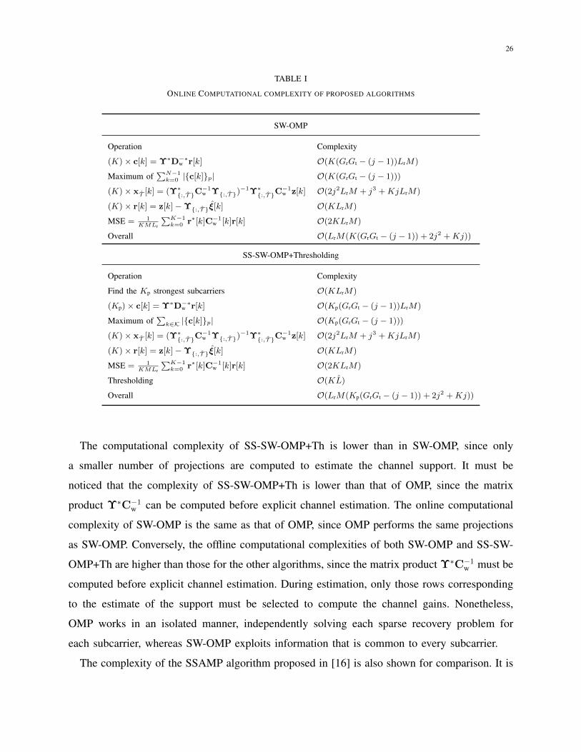
TABLE I
ONLINE COMPUTATIONAL COMPLEXITY OF PROPOSED ALGORITHMS
SW-OMP
Operation Complexity
(K)× c[k] = Υ∗D−∗w r[k] O(K(GrGt − (j − 1))LrM)
Maximum of∑N−1k=0 |c[k]p| O(K(GrGt − (j − 1)))
(K)× xT [k] = (Υ∗:,T C−1w Υ:,T )
−1Υ∗:,T C−1w z[k] O(2j2LrM + j3 +KjLrM)
(K)× r[k] = z[k]−Υ:,T ξ[k] O(KLrM)
MSE = 1KMLr
∑K−1k=0 r∗[k]C−1
w [k]r[k] O(2KLrM)
Overall O(LrM(K(GrGt − (j − 1)) + 2j2 +Kj))
SS-SW-OMP+Thresholding
Operation Complexity
Find the Kp strongest subcarriers O(KLrM)
(Kp)× c[k] = Υ∗D−∗w r[k] O(Kp(GrGt − (j − 1))LrM)
Maximum of∑k∈K |c[k]p| O(Kp(GrGt − (j − 1)))
(K)× xT [k] = (Υ∗:,T C−1w Υ:,T )
−1Υ∗:,T C−1w z[k] O(2j2LrM + j3 +KjLrM)
(K)× r[k] = z[k]−Υ:,T ξ[k] O(KLrM)
MSE = 1KMLr
∑K−1k=0 r∗[k]C−1
w [k]r[k] O(2KLrM)
Thresholding O(KL)
Overall O(LrM(Kp(GrGt − (j − 1)) + 2j2 +Kj))
The computational complexity of SS-SW-OMP+Th is lower than in SW-OMP, since only
a smaller number of projections are computed to estimate the channel support. It must be
noticed that the complexity of SS-SW-OMP+Th is lower than that of OMP, since the matrix
product Υ∗C−1w can be computed before explicit channel estimation. The online computational
complexity of SW-OMP is the same as that of OMP, since OMP performs the same projections
as SW-OMP. Conversely, the offline computational complexities of both SW-OMP and SS-SW-
OMP+Th are higher than those for the other algorithms, since the matrix product Υ∗C−1w must be
computed before explicit channel estimation. During estimation, only those rows corresponding
to the estimate of the support must be selected to compute the channel gains. Nonetheless,
OMP works in an isolated manner, independently solving each sparse recovery problem for
each subcarrier, whereas SW-OMP exploits information that is common to every subcarrier.
The complexity of the SSAMP algorithm proposed in [16] is also shown for comparison. It is

27
TABLE II
ONLINE COMPUTATIONAL COMPLEXITY OF PREVIOUSLY PROPOSED ALGORITHMS
OMP from [13]
Operation Complexity
(K)× c[k] = Υ∗[k]r[k] O(K(GrGt − (j − 1))LrM)
(K)× Maximum of |c[k]p| O(K(GrGt − (j − 1)))
(K)× xT [k] = Υ†:,T
[k]z[k] O(K(2j2LrM + j3))
(K)× r[k] = z[k]−Υ:,T [k]ξ[k] O(KLrM)
(K)×MSE = 1MLr
r∗[k]r[k] O(KLrM)
Overall O(KLrM(GrGt − (j − 1)) + 2j2)
SSAMP from [16]
Operation Complexity
(K)× ap = Φ∗pbi−1p O(KGrGtLrM)
Maximum of∑N−1p=0 ‖ap‖
22 O(NGtGr)
(K)× tpΩi−1∪Γ = ((Φp)†Ωi−1∪Γ
rp O(K(4j2MLr + (2j)3))
Prune support Ω = arg maxΩ
∑Pp=1 ‖tpΩ‖
22, |Ω| = T O(2Kj)
(K)× cpΩ = (ΦpΩ)†rp O(K(2j2MLr + j3))
(K)× bp = rp −Φpcp O(KLrMGtGr)
Computation of total error∑K−1p=0 ‖bp‖
22 O(KMLr)
Overall O(2KLrM(GrGt + 6j2))
DGMP from [17]
Operation Complexity
(K)× ap = Υ∗prp O(KGrGtLrM)
Maximum of ρ = arg maxρ
∑N−1p=0 ‖ap‖
22 O(KGtGr)
(K)× αpρ = (Φp†ρrp O(K(2j2MLr + j3))
Overall O(KLrM(GrGt + 2j2))
important to remark that this algorithm is based on the assumption that the frequency-selective
hybrid precoders and combiners used during training are semiunitary. Therefore, this algorithm
does not take into account the noise covariance matrix Cw, neither for the computation of the
channel gains nor for the estimation of the support of the sparse channel matrices.
We observe that the computational complexity of SW-OMP is lower than its SSAMP coun-
terpart. This is because SSAMP exhibits an increase in complexity of at most O(4j2) owing
28
to the estimation of j paths at the j-th iteration of SSAMP. This is because this algorithm
uses an iteration index i to estimate the sparsity level L, and a stage index j to estimate the
j channel paths found at the current iteration. Afterwards, the support of the channel estimate
is pruned to select the j most likely channel paths. Therefore, at a given iteration i and stage
j, at most 2j = |Ωi−1 ∪ Γ| paths are estimated and then pruned, such that only j paths are
selected among the 2j candidates. The union of the sets Ω and Γ comes from the possibility
of finding new potential paths at the i-th iteration and the j-th stage. This is done by jointly
considering the paths found at (i − 1)-th iteration and the ones found in the j-th stage within
the i-th iteration. Therefore, whereas both SW-OMP, SS-SW-OMP+Th and OMP estimate a
single path at a given iteration j, SSAMP estimates at most 2j different paths by using LS.
When computing the pseudoinverse during LS estimation, this results in an additional increase
in complexity of O(4j2), as shown in Table II. By contrast, as shown in Table I, our proposed
ML estimator for the channel gains exhibits computational complexity in the order of O(2j2),
thereby slightly reducing the number of operations. Further, both SW-OMP, SS-SW-OMP+Th
and OMP do not compute the projections between every column of the measurement matrix
and the received frequency-domain signals. Instead, a path that was already found in a previous
iteration is not estimated again, thereby keeping computational complexity lower than that of
SSAMP.
Last, SSAMP considers the use of K different measurement matrices for channel estimation.
As discussed in Section III, this work considers analog-only training precoders and combiners
to estimate the channel, which are constrained to be frequency flat. Consequently, the noise
covariance matrix is constant across the different subcarriers. Besides, a frequency-flat data
stream s(m) ∈ CNs×1 is transmitted at every subcarrier for a given training step m, 1 ≤ m ≤M .
Thereby, a single frequency-flat measurement matrix is used to jointly estimate the K different
subchannels. This results in a complexity reduction by a factor of K at every iteration, both
during the estimation of the support and during estimation of the channel gains. Thereby, the
entire process of estimating the channel is greatly simplified.
While OMP does not require any off-line operation, both SW-OMP and SS-SW-OMP+Th need
to compute the whitened measurement matrices Υw = D−1w Υ for the different subcarriers. The
offline computation of D−1w has complexity of O(M3L3
r ), since C−1w is a block diagonal matrix
containing M hermitian matrices. Therefore, the Cholesky decomposition of C−1w is nothing but

29
the block diagonal matrix containing the Cholesky decompositions of the covariance matrices for
the different training frames. The cost of such decomposition for a matrix A ∈ Ck×k is O(k3
3).
The overall cost is calculated taking this individual cost into account. It is important to remark
that this cost comes from the use of frequency-flat precoders/combiners and training symbols.
This entails a reduction in computational complexity with respect to the case in which frequency-
selective baseband combiners were used during the channel estimation stage. Nonetheless, in our
simulations, only analog precoders and combiners are used during the training stage, therefore
reducing the computational complexity by a factor of K.
V. CONCLUSIONS
In this paper, we proposed two compressive channel estimation approaches suitable for OFDM-
based communication systems. These two strategies are based on jointly-sparse recovery to
exploit information on the common basis that is shared for every subcarrier. Our compressive
approaches enable MIMO operation in mmWave systems since the different subchannels are
simultaneously estimated during the training phase. Further, if there is no grid quantization error
and the estimation of the support is correct, we showed that our algorithms are asymptotically
efficient since they asymptotically attain the CRLB. In simulations, we found that only a small
number of subcarriers provide a high probability of correct support detection, thus our estimators
approach the CRLB with reduced computational complexity. The approaches were also found
to work well even with off-grid parameters, and to outperform competitive frequency-domain
channel estimation approaches. For future work, it would be interesting to analytically calculate
the minimum required number of subcarriers to guarantee a high probability of correctly recov-
ering the support of the sparse channel vectors. It would also be interesting to study the effects
of other impairments including array miscalibration, beam squint, and synchronization errors.
REFERENCES
[1] T. Rappapport et al, Millimeter Wave Wireless Communications. Pearson Education, Inc., 2014.
[2] R.W. Heath, N. Gonzalez-Prelcic, S. Rangan, W. Roh, and A. M. Sayeed, ”An overview of signal processing techniques
for millimeter wave MIMO systems”, IEEE J. Sel. Areas Commun., vol. 10, no. 3, pp. 436-453, April 2016.
[3] A. Alkhateeb, J. Mo, N. Gonzalez-Prelcic, and R. W. Heath Jr., ”MIMO precoding and combining solutions for millimeter-
wave systems”, IEEE Commun. Mag., vol. 52, no. 12, pp. 122-131, Dec 2014
[4] M. L. Malloy and R. D. Nowak, ”Near-optimal adaptive compressed sensing”, in Proc. Asil. Conf. Signals, Syst. Comp.
(ASILOMAR), Pacific Grove, CA, 2012, pp. 1935-1939.
30
[5] -, ”Near-optimal compressive binary search”, arXiv preprint arXiv:1306.6239, 2012.
[6] M. Iwen and A. Tewfik, ”Adaptive strategies for target detection and localization in noisy environments”, IEEE Trans.
Signal Process., vol. 60, no. 5, pp. 2344-2353, 2012.
[7] A. Alkhateeb, O. E. Ayach, G. Leus, and R. W. Heath Jr. ”Channel estimation and hybrid precoding for millimeter wave
cellular systems”, IEEE J. Sel. Topics Signal Process., vol. 8, no. 5, pp. 831-846, Oct. 2014.
[8] D. Ramasamy, S. Venkateswaran, and U. Madhow, ”Compressive adaptation of large steerable arrays”, in Information Theory
and Applications Workshop (ITA), 2012, Feb. 2012, pp. 234-239.
[9] -, ”Compressive tracking with 1000-element arrays: A framework for multi-Gbps mm wave cellular downlinks”, in Proc.
Annual Allerton Conference on Communication, Control, and Computing, Oct. 2012, pp. 690-697.
[10] D. E. Berraki, S. M. D. Armour, and A. R. Nix, ”Application of compressive sensing in sparse spatial channel recovery for
beamforming in mmWave outdoor systems”, in Proc. IEEE Wireless Communications and Networking Conference (WCNC),
Apr. 2014, pp. 887-892.
[11] J. Lee, G. Gye-Tae, and Y. H. Lee, ”Exploiting spatial sparsity for estimating channel sof hybrid MIMO systems in
millimeter wave communications”, in Proc. IEEE Globecom, 2014.
[12] R. Mendez-Rial, C. Rusu, N. Gonzalez-Prelcic, A. Alkhateeb, and R. W. Heath Jr., ”Hybrid MIMO architectures for
millimeter wave communications”, in Proc. IEEE Globecom, 2014.
[13] K. Venugopal, A. Alkhateeb, N. Gonzalez-Prelcic, and R. W. Heath Jr., ”Time-domain channel estimation for wideband
millimeter wave systems with hybrid architecture”, in submitted to Int. Conf. Acoust. Speech and Sig. Proc. (ICASSP), Sept.
2016, pp. 1-5.
[14] K. Venugopal, A. Alkhateeb, N. Gonzalez-Prelcic, and R. W. Heath Jr., ”Channel estimation for hybrid architecture based
wideband millimeter wave systems”, IEEE Journal on Selected Areas in Communications, to appear, 2017.
[15] J. Rodrıguez-Fernandez, N. Gonzalez-Prelcic, K. Venugopal, and R. W. Heath Jr., ”A frequency-domain approach to
wideband channel estimation in millimeter wave systems”, in Proc. IEEE Int. Conf. Commun. (ICC), 2017.
[16] Z. Gao, L. Dai, and Z. Wang, ”Channel estimation for mmwave massive MIMO based access and backhaul in ultra-dense
network”, in Proc. IEEE Int. Conf. on Commun. (ICC), May 2016, pp. 1-6.
[17] Z. Gao, C. Hu, L. Dai, and Z. Wang, ”Channel estimation for millimeter-wave massive MIMO with hybrid precoding over
frequency-selective fading channels”, IEEE Communications Letters, vol. 20, no 6, pp. 1259-1262, June 2016.
[18] P. Schniter and A. Sayeed, ”Channel estimation and precoder design for millimeter-wave communications: The sparse
way”, in Proc. Asilomar Conf. Signals, Syst., Comput., Nov. 2014, pp. 273-277.
[19] A. Alkhateeb and R. W. Heath Jr., ”Freuqnecy selective hybrid precoding for limited feedback millimeter wave systems”,
IEEE Trans. Commun., vol. 64, no. 5, pp. 1801-1818, May 2016.
[20] S. G. Larew, T. A. Thomas, M. Cudak, and A. Ghosh, ”Air interface design and ray tracing study for 5g millimeter wave
communicaitons”, in Proc. IEEE Globecom Workshops (GC Wkshps), Dec. 2013.
[21] T. S. Rappaport, G. R. MacCartney, M. K. Samimi, and S. Sun, ”Wideband millimeter-wave propagation measurements
and channel models for future wireless communication system design”, IEEE Transactions on Communications, vol. 63,
no. 9, pp. 3029-3056, Sept. 2015.
[22] J. A. Tropp, A. C. Gilbert, and M. J. Strauss, ”Simultaneous sparse approximation via greedy pursuit”, in Proc. IEEE
Conf. Acous. Speech, and Signal Processing (ICASSP), 2005.
[23] S. M. Kay, Fundamentals of Statistical Signal Processing, Volume I: Estimation Theory. Prentice Hall PTR, 1993.


