arX
iv:1
203.
4156
v1 [
q-fin
.PM
] 19
Mar
201
21
Optimal Investment Under Transaction Costs:
A Threshold Rebalanced Portfolio ApproachSait Tunc and Suleyman S. Kozat,Senior Member, IEEE
Abstract
We study optimal investment in a financial market having a finite number of assets from a signal
processing perspective. We investigate how an investor should distribute capital over these assets and when
he should reallocate the distribution of the funds over these assets to maximize the cumulative wealth
over any investment period. In particular, we introduce a portfolio selection algorithm that maximizes the
expected cumulative wealth in i.i.d. two-asset discrete-time markets where the market levies proportional
transaction costs in buying and selling stocks. We achieve this using “threshold rebalanced portfolios”,
where trading occurs only if the portfolio breaches certainthresholds. Under the assumption that the
relative price sequences have log-normal distribution from the Black-Scholes model, we evaluate the
expected wealth under proportional transaction costs and find the threshold rebalanced portfolio that
achieves the maximal expected cumulative wealth over any investment period. Our derivations can be
readily extended to markets having more than two stocks, where these extensions are pointed out in the
paper. As predicted from our derivations, we significantly improve the achieved wealth over portfolio
selection algorithms from the literature on historical data sets.
Index Terms
Portfolio management, threshold rebalancing, transaction cost, discrete-time market, continuous dis-
tribution.
EDICS Category: MLR-APPL, MLR-LEAR, SSP-APPL.
This work is supported in part by IBM Faculty Award and Outstanding Young Scientist Award Program from Turkish
Academy of Sciences. Suleyman S. Kozat and Sait Tunc ({skozat,saittunc}@ku.edu.tr) are with the Competitive Signal Processing
Laboratory at the Koc University, Istanbul, 34450, tel: +902123381864, fax: +902123381548.
2
I. INTRODUCTION
Recently financial applications attracted a growing interest from the signal processing community
since the recent global crises demonstrated the importanceof sound financial modeling and reliable data
processing [1], [2]. Financial markets produce vast amountof temporal data ranging from stock prices
to interest rates, which make them ideal mediums to apply signal processing methods. Furthermore, due
to the integration of high performance, low-latency computing recourses and the financial data collection
infrastructures, signal processing algorithms could be readily leveraged with full potential in financial
stock markets. This paper particularly focuses on the portfolio selection problem, which is one the most
important financial applications and has already attractedsubstantial interest from the signal processing
community [3]–[7].
In particular, we study the investment problem in a financialmarket having a finite number of assets. We
concentrate on how an investor should distribute capital over these assets and when he should reallocate the
distribution of the funds over those assets in time to maximize the overall cumulative wealth. In financial
terms, distributing ones capital over various assets is known as the portfolio management problem and
reallocation of this distribution by buying and selling stocks is referred as the rebalancing of the given
portfolio [8]. Due to obvious reasons, the portfolio management problem has been investigated in various
different fields from financial engineering [9], machine learning to information theory [10], with a sig-
nificant room for improvement as the recent financial crises demonstrated. To this end, we investigate the
portfolio management problem in discrete-time markets when the market levies proportionaltransaction
costsin trading while buying and selling stocks, which accurately models a wide range of real life markets
[8], [9]. In discrete time markets, we have a finite number of assets and the reallocation of wealth (or
rebalancing of the capital) over these assets is only allowed at discrete investment periods, where the
investment period is arbitrary, e.g., each second, minute or each day [10], [11]. Under this framework, we
introduce algorithms that achieve themaximalexpected cumulative wealth under proportional transaction
costs in i.i.d. discrete-time markets extensively studiedin the financial literature [8], [9]. We further
illustrate that our algorithms significantly improve the achieved wealth over the well-known algorithms
in the literature on historical data sets under realistic transaction costs, as anticipated from our derivations.
The precise problem description including the market and transaction cost models are provided in Section
III.
Determination of the optimum portfolio and the best portfolio rebalancing strategy that maximize
the wealth in discrete-time markets withno transaction feesis heavily investigated in information theory
3
[10], [11], machine learning [12]–[14] and signal processing [15]–[18] fields. Assuming that the portfolio
rebalancings, i.e., adjustments by buying and selling stocks, require no transaction fees and with some
further mild assumptions on the stock prices, the portfoliothat achieves the maximum wealth is shown to
be a constant rebalanced portfolio (CRP) [11], [19]. A CRP isa portfolio strategy where the distribution
of funds over the stocks are reallocated to a predetermined structure, also known as the target portfolio,
at the start of each investment period. CRPs constitute a subclass of a more general portfolio rebalancing
class, the calendar rebalancing portfolios, where the portfolio vector is rebalanced to a target vector
on a periodic basis [8]. Numerous studies are carried out to asymptotically achieve the performance of
the best CRP tuned to the individual sequence of stock pricesalbeit either with different performance
bounds or different performance results on historical datasets [11], [12], [14]. CRPs under transaction
costs are further investigated in [20], where a sequential algorithm using a weighting similar to that
introduced in [19], is also shown to be competitive under transaction costs, i.e., asymptotically achieving
the performance of the best CRP under transaction costs. However, we emphasize that maintaining a
CRP requires potentially significant trading due to possible rebalancings at each investment period [15].
As shown in [15], even the performance of the best CRP is severally affected by moderate transaction
fees rendering CRPs ineffective in real life stock markets.Hence, it may not be enough to try to achieve
the performance of the best CRP if the cost of rebalancing outweighs that which could be gained from
rebalancing at every investment period. Clearly, one can potentially obtain significant gain in wealth by
including unavoidable transactions fees in the market model and perform reallocation accordingly.
In these lines, the optimal portfolio selection problem under transactions costs is extensively investigated
for continuous-time markets [21]–[24], where growth optimal policies that keep the portfolio in closed
compact sets by trading only when the portfolio hits the compact set-boundaries are introduced. Naturally,
the results for the continuous markets cannot be straightforwardly extended to the discrete-time markets,
where continuous trading is not allowed. However, it has been shown in [25] that under certain mild
assumptions on the sequence of stock prices, similar no trade zone portfolios achieve the optimal growth
rate even for discrete-time markets under proportional transaction costs. For markets having two stocks,
i.e., two-asset stock markets, these no trade zone portfolios correspond to threshold portfolios, i.e., the
no trade zone is defined by thresholds around the target portfolio. As an example, for a market with two
stocks, the portfolio is represented by a vectorb = [b 1− b]T , b ∈ [0, 1], assuming only long positions
[8], whereb is the ratio of the capital invested in the first stock. For this market, the no rebalancing region
around a target portfoliob = [b 1−b]T , b ∈ [0, 1], is given by a thresholdǫ, min{b, 1−b} ≥ ǫ ≥ 0, such
that the corresponding portfolio at any investment period is rebalanced to a desired vector if the ratio of

4
the wealth in the first stock breaches the interval(b− ǫ, b+ ǫ). In particular, unlike a calendar rebalancing
portfolio, e.g., a CRP, a threshold rebalanced portfolio (TRP) rebalances by buying and selling stocks
only when the portfolio breaches the preset boundaries, or “thresholds”, and otherwise does not perform
any rebalancing. Intuitively, by limiting the number of rebalancings due to this non rebalancing regions,
threshold portfolios are able to avoid hefty transactions costs associated with excessive trading unlike
calendar portfolios. Although TRPs are shown to be optimal in i.i.d. discrete-time two-asset markets
(under certain technical conditions) [25], finding the TRP that maximizes the expected growth of wealth
under proportional transaction costs is not solved, exceptfor basic scenarios [25], to the best of our
knowledge.
In this paper, we first evaluate the expected wealth achievedby a TRP over any finite investment period
given any target portfolio and threshold for two-asset discrete-time stock markets subject to proportional
transaction fees. We emphasize that we study two-asset market for notational simplicity and our derivations
can be readily extended to markets having more than two assets as pointed out in the paper where
needed. We consider i.i.d. discrete-time markets represented by the sequence of price relatives (defined
as the ratio of the opening price to the closing price of stocks), where the sequence of price relatives
follow log-normal distributions. Note that the log-normaldistribution is the assumed statistical model
for price relative vectors in the well-known Black-Scholesmodel [8], [9] and this distribution is shown
to accurately model real life stock prices by many empiricalstudies [8]. Under this setup, we provide
an iterative relation that efficiently and recursively calculates the expected wealth over any period in
any i.i.d. discrete time market. This iterative relation is evaluated using a certain multivariate Gaussian
integral for the log-normal distribution. We then provide arandomized algorithm to calculate the given
integral and obtain the expected growth. This expected growth is then optimized by a brute force method
to yield the optimal target portfolio and threshold to maximize the expected wealth over any investment
period. Furthermore, we also provide a maximum-likelihoodestimator to estimate the parameters of
the log-normal distribution from the sequence of price relative vectors, which is incorporated into the
algorithmic framework in Simulations section since these parameters are naturally unknown in real life
markets.
Portfolio management problem is studied with transaction costs in [26] on the horse race setting, which
is a special discrete-time market where only one of the assetpays off and the others pay nothing on each
period. This basic framework is then extended to general stock markets in [25], where threshold portfolios
are shown to be growth optimal for two-asset markets. However, no algorithm, except for a special sampled
Brownian market, is provided to find the optimal target portfolio or threshold in [25]. To achieve the
5
performance of the best TRP, a sequential algorithm is introduced in [27] that is shown to asymptotically
achieve the performance of the best TRP tuned to the underlying sequence of price relatives. This
algorithm uses a similar weighting introduced in [19] to construct the universal portfolio. We emphasize
that the universal investment strategies, e.g., [27], which are inspired by universal source coding ideas,
based on Bayesian type weighting, are heavily utilized to construct sequential investment strategies [3],
[5], [11], [13]–[18]. Although these methods are shown to “asymptotically” achieve the performance of
the best portfolio in the competition class of portfolios, their non-asymptotic performance is acceptable
only if a sufficient number of candidate algorithms in the competition class is overly successful [15] to
circumvent the loss due to Bayesian type averaging. Since these algorithms are usually designed in a min-
max (or universal) framework and hedge against (or should even work for) the worst case sequence, their
average (or generic) performance may substantially suffer[12], [28], [29]. In our simulations, we show
that our introduced algorithm readily outperforms a wide class of universal algorithms on the historical
data sets, including [27]. Note that to reduce the negative effect of the transaction costs in discrete time
markets, semiconstant rebalanced portfolio (SCRP) strategies have also been proposed and studied in
[12], [15], [20]. Different than a CRP and similar to the TRPs, an SCRP rebalances the portfolio only at
the determined periods instead of rebalancing at the start of each period. Since for an SCRP algorithm
rebalancing occurs less frequently than a CRP, using an SCRPstrategy may improve the performance over
CRPs when transaction fees are present. However, no formulation exists to find the optimal rebalancing
times for SCRPs to maximize the cumulative wealth. Althoughthere exist universal methods [13], [15]
that achieve asymptotically the performance of the best SCRP tuned to the underlying sequence of price
relatives, these methods suffer in realistic markets sincethey are tuned to the worst case scenario [15]
as demonstrated in the Simulations section.
We begin with the detailed description of the market and the TRPs in Section II. We then calculate the
expected wealth using a TRP in an i.i.d. two-asset discrete-time market under proportional transaction
costs over any investment period in Section III. We first provide an iterative relation to recursively
calculate the expected wealth growth. The terms in the iterative algorithm are calculated using a certain
form of multivariate Gaussian integrals. We provide a randomized algorithm to calculate these integrals
in Section III-C. The maximum-likelihood estimation of theparameters of the log-normal distribution is
given in Section IV. The paper is then concluded with the simulations of the iterative relation and the
optimization of the expected wealth growth with respect to the TRP parameters using the ML estimator
in Section V.

6
II. PROBLEM DESCRIPTION
In this paper, all vectors are column vectors and represented by lower-case bold letters. Consider a
market withm stocks and let{x(t)}t≥1 represent the sequence of price relative vectors in this market,
wherex(t) = [x1(t), x2(t), . . . , xm(t)]T with xi(t) ∈ R+ for i ∈ {1, 2, . . . ,m} such thatxi(t) represents
the ratio of the closing price of theith stock for thetth trading period to that from the(t− 1)th trading
period. At each investment period, say periodt, b(t) represents the vector of portfolios such thatbi(t) is
the fraction of money invested on theith stock. We allow only long-trading such that∑m
i=1 bi(t) = 1 and
bi(t) ≥ 0. After the price relative vectorx(t) is revealed, we earnbT (t)x(t) at the periodt. Assuming
we started investing using 1 dollars, at the end ofn periods, the wealth growth in a market with no
transaction costs is given by
S(n) =
n∏
t=1
bT (t)x(t). (1)
If we use a CRP [10], then we earnn∏
t=1
bTx(t),
at the end ofn periods ignoring the transaction costs. This method is called “constant rebalancing” since
at the start of each investment periodt, the portfolio vectorb(t) = [b1(t), b2(t), . . . , bm(t)] is adjusted,
or rebalanced, to a predetermined constant portfolio vector, say,b = [b1, b2, . . . , bm] where∑m
i=1 bi = 1.
As an example, at the start of each investment periodt, since we invested usingb at the investment
period t− 1 and observedx(t− 1), the current portfolio vector, saybold(t),
bold(t)△=
[
b1x1(t− 1)∑m
i=1 bixi(t− 1), . . . ,
bmxm(t− 1)∑m
i=1 bixi(t− 1)
]T
,
should be adjusted back tob. If we assume a symmetric proportional transaction cost with cost ratioc, 0 ≤
c ≤ 1, for both selling and buying, then we need to spend approximately∑m
i=1 bi,old(t)S(t)|bi,old(t)−bi|c
dollars for rebalancing. Note that if the transaction costsare not symmetric, the analysis follows by
assumingc = csell + cbuy by [20], wherecsell and cbuy are the proportional transaction costs in selling
and buying, respectively. Since a CRP should be rebalanced back to its initial value at the start of each
investment period, a transaction fee proportional to the wealth growth up to the current period, i.e.,S(t),
is required for each periodt. Hence, constantly rebalancing at each timet may be unappealing for large
c.
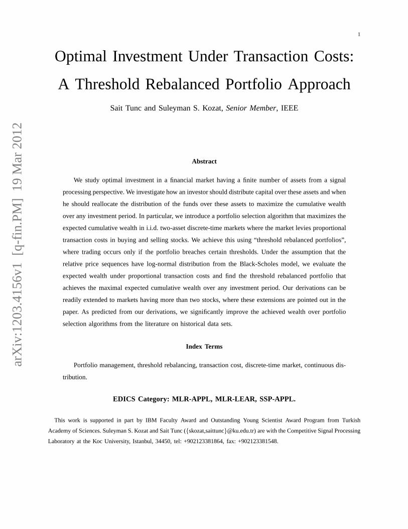
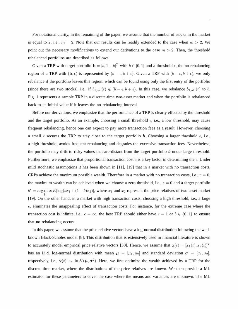
To avoid such frequent rebalancing, we use TRPs, where we denote a TRP with a target vectorb and
a thresholdǫ (with certain abuse of notation) as “TRP with(b, ǫ)”. For a sequence of price relatives

7
!"#$"%&"'()%*+'
,-.+/01+-0'!+#&"2'
34506'
0'
3'
378'
398'
4' :' ;' <' =' >' ?' @' A' 4B'
Fig. 1: A sample scenario for threshold rebalanced portfolios.
vectorsxn △= [x(1),x(2), . . . ,x(n)] with x ∈ R+
m, a TRP with(b, ǫ) rebalances the portfolio tob at the
first time τ satisfying
bj∏τ
t=1 xj(t)∑m
k=1 bk∏τ
t=1 xk(t)/∈ [bj − ǫj , bj + ǫj] (2)
for anyj ∈ {1, 2, . . . ,m}, thresholdsǫj , and does not rebalance otherwise, i.e., while the portfolio vector
stays in the no rebalancing region. Starting from the first period of a no rebalancing region, i.e., where
the portfolio is rebalanced to the target portfoliob, sayt = 1 for this example, the wealth gained during
any no rebalancing region is given by
W (xn|bn ∈ Encn ) =
m∑
k=1
bk
n∏
t=1
xk(t), (3)
wherebn = [b(1),b(2), . . . ,b(n)] with b(t) is the portfolio at periodt and Enc
n is the lengthn no
rebalancing region defined as
Encn = {bn | b(1) = b, bj(t) ∈ (bj − ǫj, bj + ǫj), j ∈ {1, 2, . . . ,m}, t ∈ {1, 2, . . . , n}}. (4)
A TRP pays a transaction fee when the portfolio vector leavesthe predefined no rebalancing region, i.e.,
goes out of the no rebalancing regionEncn , and rebalanced back to its target portfolio vectorb. Since the
TRP may avoid constant rebalancing, it may avoid excessive transaction fees while securing the portfolio
to stay close the target portfoliob, when we have heavy transaction costs in the market.
8
For notational clarity, in the remaining of the paper, we assume that the number of stocks in the market
is equal to 2, i.e.,m = 2. Note that our results can be readily extended to the case when m > 2. We
point out the necessary modifications to extend our derivations to the casem > 2. Then, the threshold
rebalanced portfolios are described as follows.
Given a TRP with target portfoliob = [b, 1− b]T with b ∈ [0, 1] and a thresholdǫ, the no rebalancing
region of a TRP with(b, ǫ) is represented by(b − ǫ, b + ǫ). Given a TRP with(b − ǫ, b + ǫ), we only
rebalance if the portfolio leaves this region, which can be found using only the first entry of the portfolio
(since there are two stocks), i.e., ifb1,old(t) /∈ (b − ǫ, b + ǫ). In this case, we rebalanceb1,old(t) to b.
Fig. 1 represents a sample TRP in a discrete-time two-asset market and when the portfolio is rebalanced
back to its initial value if it leaves the no rebalancing interval.
Before our derivations, we emphasize that the performance of a TRP is clearly effected by the threshold
and the target portfolio. As an example, choosing a small thresholdǫ, i.e., a low threshold, may cause
frequent rebalancing, hence one can expect to pay more transaction fees as a result. However, choosing
a small ǫ secures the TRP to stay close to the target portfoliob. Choosing a larger thresholdǫ, i.e.,
a high threshold, avoids frequent rebalancing and degradesthe excessive transaction fees. Nevertheless,
the portfolio may drift to risky values that are distant fromthe target portfoliob under large threshold.
Furthermore, we emphasize that proportional transaction costc is a key factor in determining theǫ. Under
mild stochastic assumptions it has been shown in [11], [19] that in a market with no transaction costs,
CRPs achieve the maximum possible wealth. Therefore in a market with no transaction costs, i.e.,c = 0,
the maximum wealth can be achieved when we choose a zero threshold, i.e.,ǫ = 0 and a target portfolio
b∗ = argmaxb
E[log(bx1+(1− b)x2)], wherex1 andx2 represent the price relatives of two-asset market
[19]. On the other hand, in a market with high transaction costs, choosing a high threshold, i.e., a large
ǫ, eliminates the unappealing effect of transaction costs. For instance, for the extreme case where the
transaction cost is infinite, i.e.,c = ∞, the best TRP should either haveǫ = 1 or b ∈ {0, 1} to ensure
that no rebalancing occurs.
In this paper, we assume that the price relative vectors havea log-normal distribution following the well-
known Black-Scholes model [8]. This distribution that is extensively used in financial literature is shown
to accurately model empirical price relative vectors [30].Hence, we assume thatx(t) = [x1(t), x2(t)]T
has an i.i.d. log-normal distribution with meanµ = [µ1, µ2] and standard deviationσ = [σ1, σ2],
respectively, i.e.,x(t) ∼ lnN (µ,σ2). Here, we first optimize the wealth achieved by a TRP for the
discrete-time market, where the distributions of the pricerelatives are known. We then provide a ML
estimator for these parameters to cover the case where the means and variances are unknown. The ML
9
estimator is incorporated in the algorithmic framework in the Simulations section since the corresponding
parameters are unknown in real life markets. The details of the maximum-likelihood estimation are given
in Section IV.
III. T HRESHOLD REBALANCED PORTFOLIOS
In this section, we analyze the TRPs in a discrete-time market with proportional transaction costs as
defined in Section II. We first introduce an iterative relation, as a theorem, to recursively evaluate the
expected achieved wealth of a TRP over any investment period. The terms in this iterative equation are
calculated using a certain form of multivariate Gaussian integrals. We provide a randomized algorithm
to calculate these integrals. We then use the given iterative equation to find the optimalǫ and b that
maximize the expected wealth over any investment period.
A. An Iterative Relation to Calculate the Expected Wealth
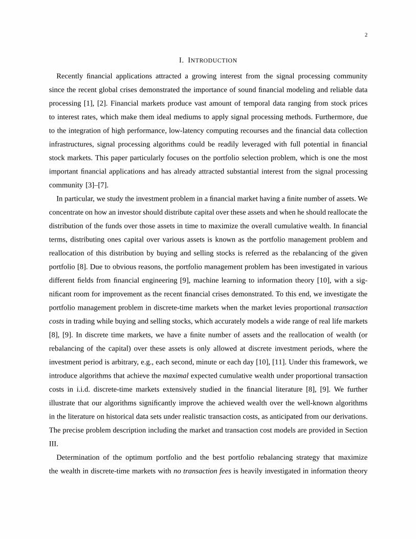
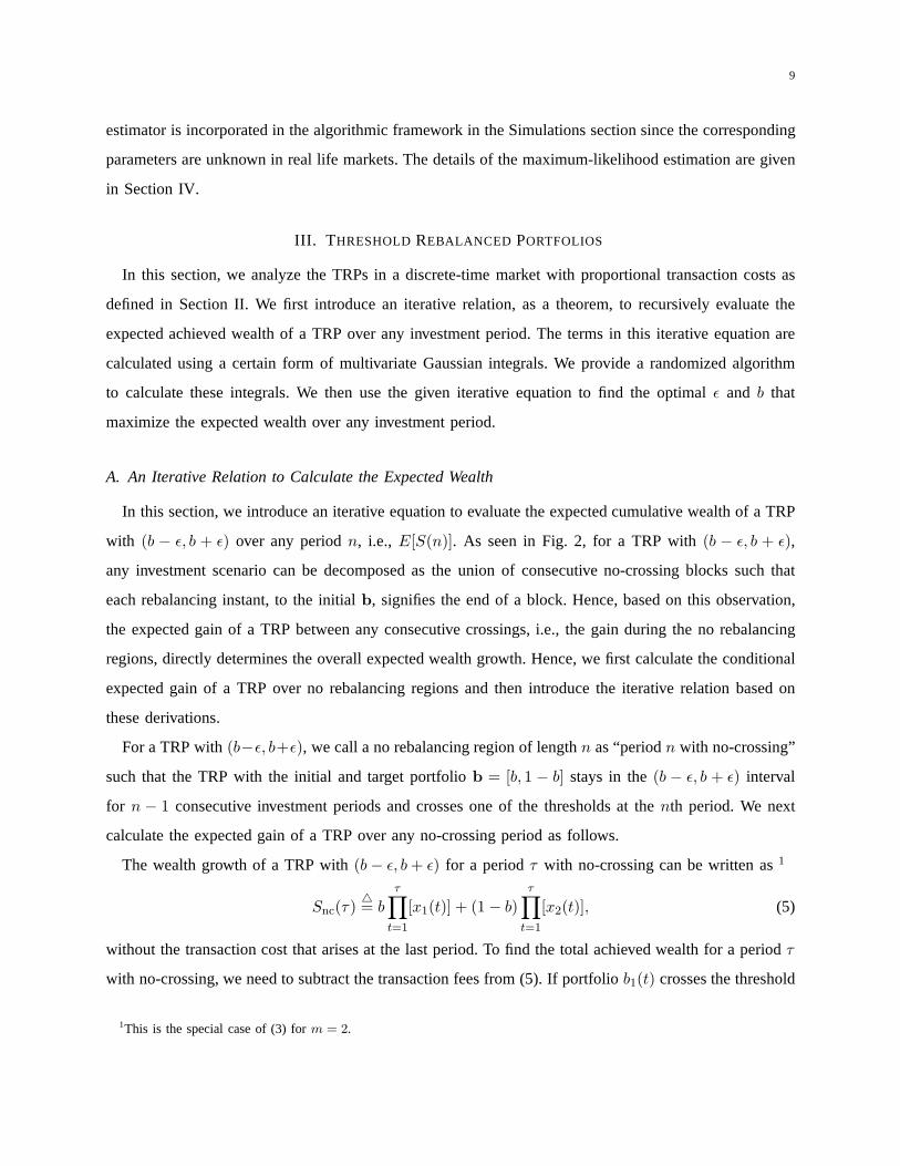
In this section, we introduce an iterative equation to evaluate the expected cumulative wealth of a TRP
with (b − ǫ, b + ǫ) over any periodn, i.e., E[S(n)]. As seen in Fig. 2, for a TRP with(b − ǫ, b + ǫ),
any investment scenario can be decomposed as the union of consecutive no-crossing blocks such that
each rebalancing instant, to the initialb, signifies the end of a block. Hence, based on this observation,
the expected gain of a TRP between any consecutive crossings, i.e., the gain during the no rebalancing
regions, directly determines the overall expected wealth growth. Hence, we first calculate the conditional
expected gain of a TRP over no rebalancing regions and then introduce the iterative relation based on
these derivations.
For a TRP with(b−ǫ, b+ǫ), we call a no rebalancing region of lengthn as “periodn with no-crossing”
such that the TRP with the initial and target portfoliob = [b, 1 − b] stays in the(b − ǫ, b + ǫ) interval
for n − 1 consecutive investment periods and crosses one of the thresholds at thenth period. We next
calculate the expected gain of a TRP over any no-crossing period as follows.
The wealth growth of a TRP with(b− ǫ, b+ ǫ) for a periodτ with no-crossing can be written as1
Snc(τ)△= b
τ∏
t=1
[x1(t)] + (1− b)
τ∏
t=1
[x2(t)], (5)
without the transaction cost that arises at the last period.To find the total achieved wealth for a periodτ
with no-crossing, we need to subtract the transaction fees from (5). If portfolio b1(t) crosses the threshold
1This is the special case of (3) form = 2.

10
at the investment periodt = τ , then we need to rebalance it back tob, i.e., b1(t) = b and pay
Snc(τ)c
∣
∣
∣
∣
b∏τ
t=1(x1(t))
b∏τ
t=1(x1(t)) + (1− b)∏τ
t=1(x2(t))− b
∣
∣
∣
∣
, (6)
wherec represents the symmetrical commission cost, to rebalance two stocks, i.e.,b1,old(τ +1) to b, and
b2,old(τ + 1) = 1 − b1,old(τ + 1) to 1 − b. Hence, the net overall gain for a periodτ with no-crossing
becomes
S(τ) = Snc(τ)− Snc(τ)c
∣
∣
∣
∣
b∏τ
t=1(x1(t))
b∏τ
t=1(x1(t)) + (1− b)∏τ
t=1(x2(t))− b
∣
∣
∣
∣
= b
τ∏
t=1
[x1(t)] + (1− b)
τ∏
t=1
[x2(t)]− c(b− b2)
∣
∣
∣
∣
∣
τ∏
t=1
[x1(t)]−τ∏
t=1
[x2(t)]
∣
∣
∣
∣
∣
= ζ1
τ∏
t=1
[x1(t)] + ζ2
τ∏
t=1
[x2(t)], (7)
whereζ1△= b − 2c(b − b2) and ζ2
△= 1 − b + 2c(b − b2) for b + ǫ hitting andζ1
△= b + 2c(b − b2) and
ζ2△= 1 − b − 2c(b − b2) for b − ǫ hitting. Thus, the conditional expected gain of a TRP conditioned
on that the portfolio stays in a no rebalancing region until the last period of the region can be found
by calculating the expected value of (7). Since, we now have the conditional expected gains, we next
introduce an iterative relation to find the expected wealth growth of a TRP with(b− ǫ, b+ ǫ) for period
n, E[S(n)], by using the expected gains of no-crossing periods as shownin Fig. 2.
In order to calculate the expected wealthE[S(n)] iteratively, let us first define the variableR(τ), which
is the expected cumulative gain of all possible portfolios that hit any of the thresholds first time at the
τ th period, i.e.,
R(τ) = E[
S(τ)∣
∣
∣bτ ∈ E fc
τ
]
, (8)
whereE fcτ denotes the set of all possible portfolios with initial portfolio b and that stay in the no rebalancing
region forτ − 1 consecutive periods and hits one of theb− ǫ or b+ ǫ boundary at theτ th period, i.e.,
E fcτ
△= {bτ ∈ Bτ (b, ǫ) | b(1) = b, b(i) ∈ (b− ǫ, b+ ǫ)∀i ∈ {2, . . . , τ − 1}, b(τ) /∈ (b− ǫ, b+ ǫ)}. (9)
Here,Bτ (b, ǫ) is defined as the set of all possible threshold rebalanced portfolios with initial and target
portfolio b and a no rebalancing interval(b− ǫ, b + ǫ). Similarly we define the variableT (τ), which is
the expected growth of all possible portfolios of lengthτ with no threshold crossings, i.e.,
T (τ) = E[
S(τ)∣
∣
∣bτ ∈ Enc
τ
]
, (10)
11
!"#$"%&"'()%*+'
,-.+/01+-0'!+#&"2'
34506'
0'
3'
378'
398'
4' :' ;4' ;47;:7;<';47;:';474'=' =' ='
>'>'>''' >'>'>''' >'>'>'''
?+#&"2'"@'%+-A0B'
;4'C&0B''
-"9D#"//&-A''
?+#&"2'"@'%+-A0B';:'C&0B''
-"9D#"//&-A''
?+#&"2'"@'%+-A0B';<'
'C&0B''
-"9D#"//&-A''
Fig. 2: No-crossing intervals of threshold rebalanced portfolios.
whereEncτ denotes the set of portfolios with initial portfoliob and that stay in the no rebalancing region
for τ consecutive periods, i.e.,2
Encτ
△= {bτ ∈ Bτ (b, ǫ) | b(1) = b, b(i) ∈ [b− ǫ, b+ ǫ]∀i ∈ {2, . . . , τ}}. (11)
Given the variablesR(τ) andT (τ), we next introduce a theorem that iteratively calculates the expected
wealth growth of a TRP over any periodn. Hence, to calculate the expected achieved wealth, it is sufficient
to calculateR(τ), T (τ), threshold crossing probabilitiesP(
bn ∈ E fc
n
)
and P (bn ∈ Encn ), which are
explicitly evaluated in the next section.
Theorem 3.1: The expected wealth growth of a TRP(b − ǫ, b + ǫ), i.e., E[S(n)], over any i.i.d.
sequence of price relative vectorsxn = [x(1),x(2), . . . ,x(n)], satisfies
E[S(n)] =
n∑
i=1
P (E fci )R(i)E[S(n − i)] + P (Enc
n )T (n), (12)
where we defineS0 = 1, R(n) in (8), T (n) in (10), E fci in (11) andEnc
n in (9).
2This is the special case of the definition in (4) form = 2.
12
We emphasize that by Theorem 3.1, we can recursively calculate the expected growth of any TRP over
any i.i.d. discrete-time market under proportional transaction costs. Theorem 3.1 holds for i.i.d. markets
having eitherm = 2 or m > 2 provided that the corresponding terms in (12) can be calculated.
Proof: By using the law of total expectation [31],E[S(n)] can be written as
E[S(n)] =
∫
bn∈Bn(b,ǫ)E[S(n)|bn]P (bn)dbn, (13)
whereBn(b, ǫ) is defined as the set of all possible TRPs with the initial and target portfolio b and
thresholdǫ. To obtain (12), we consider all possible portfolios as a union of n+ 1 disjoint sets: (1) the
portfolios which cross one of the thresholds first time at the1st period; (2) the portfolios which cross
one of the thresholds first time at the2nd period; and continuing in this manner, (3) the portfolioswhich
cross one of the thresholds first time at thenth period; and finally (4) the portfolios which do not cross
the thresholds forn consecutive periods. Clearly these market portfolio sets are disjoint and their union
provides all possible portfolio paths. Hence (13) can also be written as
E[S(n)] =
n∑
i=1
∫
bi1∈E fc
i ,bni+1∈Bn−i(b,ǫ)
E[S(n)|bi1 ∈ E fc
i ,bni+1 ∈ Bn−i(b, ǫ)]P (bi
1 ∈ E fci ,b
ni+1 ∈ Bn−i(b, ǫ))db
n
+
∫
bn∈Encn
E[S(n)|bn ∈ Encn ]P (bn ∈ Enc
n )dbn, (14)
wherebji
△= [b(i), b(i + 1), . . . , b(j)]. To continue with our derivations, we defineSi→j as the wealth
growth from the periodi to period j, i.e., Si→j△= S(j)
S(i) . Assume that in the periodτ , the portfolio
crosses one of the thresholds and a rebalancing occurs. In that case, regardless of the portfolios before
the periodτ , the portfolio is rebalanced back to its initial value in theτ th period, i.e., to[b, 1 − b]T .
Since the price relative vectors are independent over time,we can conclude that the portfolios before
the periodτ are independent from the portfolios after the periodτ , i.e., b(τ) = b and every portfolio
b(i) for i ∈ {1, 2, . . . , τ − 1} are independent from the portfoliosb(j) for j ∈ {τ + 1, τ + 2, . . . , n}.
Hence, the investment period where the portfolio path crosses one of the thresholds, i.e.,τ , divides the
whole investment block into uncorrelated blocks in terms ofprice relative vectors and portfolios. Thus,
the wealth growth acquired up to the periodτ , S1→τ , is uncorrelated to the wealth growth acquired after
that period, i.e.,Sτ+1→n. Hence, if we assume that a threshold crossing occurs at the period τ , then we
have
E[
S(n)|bτ1 ∈ E fc
τ ,bnτ+1 ∈ Bn−τ (b, ǫ)
]
= E[
S1→τSτ+1→n|bτ1 ∈ E fc
τ ,bnτ+1 ∈ Bn−τ (b, ǫ)
]
= E[
S1→τ |bi1 ∈ E fc
i
]
E[
Sτ+1→n|bni+1 ∈ Bn−i(b, ǫ)
]
. (15)

13
Applying (15) to (14), we get
E [S(n)] =
n∑
i=1
∫
bi1∈E fc
i ,bni+1∈Bn−i(b,ǫ)
E[
S1→i|bi1 ∈ E fc
i
]
E[
Si+1→n|b(i) = b,bni+1 ∈ Bn−i(b, ǫ)
]
P(
bi1 ∈ E fc
i
)
× P(
bni+1 ∈ Bn−i(b, ǫ)
)
dbn +
∫
bn∈Encn
E [S(n)|bn ∈ Encn ]P (bn ∈ Enc
n ) dbn. (16)
Since the integral in (16) can be decomposed into two disjoint integrals, (14) yields
E[S(n)] =
n∑
i=1
∫
bi1∈E fc
i
E[S1→i|bi1 ∈ E fc
i ]P (bi1 ∈ E fc
i )dbi1
∫
bni+1∈Bn−i(b,ǫ)
E[Si+1→n|b(i) = b,bni+1 ∈ Bn−i(b, ǫ)]
× P (bni+1 ∈ Bn−i(b, ǫ))db
ni+1 +
∫
bn∈Encn
E[S(n)|bn ∈ Encn ]P (bn ∈ Enc
n )dbn. (17)
We next write (17) as a recursive equation.
To accomplish this, we first note that
(i) R(i) is defined as the expected gain of TRPs with lengthi, which crosses one of the thresholds first
time at thei-th period and it follows that
R(i) = E[
S(τ)∣
∣
∣bi ∈ E fc
i
]
(18)
=1
P (E fci )
∫
bi1∈E fc
i
E[S1→i|bi1 ∈ E fc
i ]P (bi1 ∈ E fc
i )dbi1, (19)
where we writeP (E fci ) instead ofP (bi
1 ∈ E fci ).
(ii) Then, as the second term,T (n) is defined as the expected gain of TRPs of lengthn, which does not
cross one of the thresholds forn consecutive periods. This yields
T (n) = E[
S(n)∣
∣
∣bn ∈ Enc
n
]
(20)
=1
P (Encn )
∫
bn∈Encn
E[S(n)|bn ∈ Encn ]p(bn ∈ Enc
n )dbn. (21)
(iii) Finally, observe that the second integral in (17) is the expected wealth growth of a TRP of length
n− i, i.e.,
E[S(n − i)] =
∫
bni+1∈Bn−i(b,ǫ)
E[Si+1→n|b(i) = b,bni+1 ∈ Bn−i(b, ǫ)]p(b
ni+1 ∈ Bn−i(b, ǫ))db
ni+1, (22)
wherep(bni+1 ∈ Bn−i(b, ǫ)) = 1 by the definition of the setBn−i(b, ǫ).
Hence, if we apply (19), (21) and (22) to (17), we can write (12) as
E[S(n)] =
n∑
i=1
P (E fci )R(i)E[S(n − i)] + P (Enc
n )T (n), (23)
hence the proof concludes.

14
Theorem 3.1 provides a recursion to iteratively calculate the expected wealth growthE[S(n)], when
R(τ) andT (τ) are explicitly calculated for a TRP with(b−ǫ, b+ǫ). Hence, if we can obtainP(
E fcτ
)
R(τ)
andP (Encτ )T (τ) for any τ , then (12) yields a simple iteration that provides the expected wealth growth
for any periodn. We next give the explicit definitions of the eventsE fcτ and Enc
τ in order to calculate
the conditional expectationsR(τ) andT (τ). Following these definitions, we calculateP(
E fcτ
)
R(τ) and
P (Encτ )T (τ) to evaluate the expected wealth growthE[S(τ)], iteratively from Theorem 3.1 and find the
the optimal TRP, i.e., optimalb andǫ, by using a brute force search.
In the next section, we provide the explicit definitions forE fcτ andEnc
τ , and define the conditions for
staying in the no rebalancing region or hitting one of the boundaries to find the corresponding probabilities
of these events.
B. Explicit Calculations ofR(n) and T (n)
In this section, we first define the conditions for the market portfolios to cross the corresponding
thresholds and calculate the probabilities for the eventsE fcτ andEnc
τ . We then calculate the conditional
expectationsR(n) andT (n) as certain multivariate Gaussian integrals. The explicit calculation of mul-
tivariate Gaussian integrals are given in Section III-C.
To get the explicit definitions of the eventsE fcτ andEnc
τ , we note that we have two different boundary
hitting scenarios for a TRP, i.e., starting from the initialportfolio b, the portfolio can hitb− ǫ or b+ ǫ.
From b, the portfolio crossesb− ǫ boundary if
b∏τ
t=1(x1(t))
b∏τ
t=1(x1(t)) + (1− b)∏τ
t=1(x2(t))≤ b− ǫ, (24)
whereτ is the first time the crossing happens without ever hitting any of the boundaries before. Since
x1(i), x2(i) > 0 for all i, (24) happens ifτ∏
t=1
x2(t)
x1(t)≥
b(1− b+ ǫ)
(1− b)(b− ǫ), (25)
which is equivalent to
Π2(τ) ≥ γ1Π1(τ),
whereΠ1(i)△=
∏it=1 x1(t), Π2(i)
△=
∏it=1 x2(t) and γ1
△= b(1−b+ǫ)
(1−b)(b−ǫ) . Sincex(i)’s have log-normal
distributions, i.e.,x(t) ∼ lnN (µ,σ2), Π1(i) andΠ2(i) are log-normal, too [31]. Furthermore, to calculate

15
the required probabilities, we have
p (Π1(i),Π1(k − 1),Π1(k)) = p (Π1(i),Π1(k − 1)) p (Π1(k)|Π1(k − 1),Π1(i))
= p (Π1(i)) p (Π1(k − 1)|Π1(i)) p (Π1(k − 1)x1(k)|Π1(k − 1),Π1(i))
= p (Π1(i)) p (Π1(k − 1)|Π1(i)) p (Π1(k)|Π1(k − 1)) , (26)
∀i ∈ {0, 1, . . . , k − 2}, where (26) follows sincex(k) is independent ofΠ1(i) for k > i. HenceΠ1(i)’s
form a Markov chain such thatΠ1(i) ↔ Π1(k − 1) ↔ Π1(k) ∀i ∈ {0, 1, . . . , k − 2}. Following the
similar, steps we also obtain thatΠ2(i) ↔ Π2(k−1) ↔ Π2(k) ,∀i ∈ {0, 1, . . . , k−2}. We point out that
by extending the definitionsΠ1 andΠ2 one can obtainΠ1,Π2, . . . ,Πm for the casem > 2. Furthermore,
taking the logarithm of both sides of (25) we have
Στ1
△=
τ∑
t=1
z(t) ≥ θ1,
where z(t)△= ln
(
x2(t)x1(t)
)
and θ1△= ln b(1−b+ǫ)
(1−b)(b−ǫ) = ln γ1. The partial sums ofz(t)’s are defined as
Σki =
∑kt=i z(t) for notational simplicity. Sincex(t) ∼ lnN (µ,σ2), z(t)’s are Gaussian, i.e.,z(t) ∼
N (µ, σ2), whereµ = µ2 − µ1 andσ2 = σ21 + σ2
2 , their sums,Σki ’s, are Gaussian too. Furthermore note
that,Σk1 =
∑kt=1 z(t) =
∑kt=1 ln
(
x2(t)x1(t)
)
= ln(
∏kt=1
x2(t)x1(t)
)
= ln Π2(k)Π1(k)
.
Similarly with an initial valueb, market portfolio crossesb+ ǫ boundary if
b∏τ
t=1(x1(t))
b∏τ
t=1(x1(t)) + (1− b)∏τ
t=1(x2(t))≥ b+ ǫ, (27)
where τ is the first crossing time without ever hitting any of the boundaries before. Again, since
x1(i), x2(i) > 0 for all i, (27) happens ifτ∏
t=1
x2(t)
x1(t)≤
b(1− b− ǫ)
(1− b)(b+ ǫ), (28)
which can be written of the form
Π2(t) ≤ γ2Π1(t).
Equation (28) yields
Στ1 =
τ∑
t=1
z(t) ≤ θ2,
whereθ2△= ln b(1−b−ǫ)
(1−b)(b+ǫ) = ln γ2.
Hence, we can explicitly describe the event that the market threshold portfolio(b− ǫ, b+ ǫ) does not
hit any of the thresholds forτ consecutive periods,Encτ , as the intersection of the events as
Encτ
△=
τ⋂
i=1
{Σi1 ∈ [θ2, θ1]} =
τ⋂
i=1
{γ2Π1(i) ≤ Π2(i) ≤ γ1Π1(i)}. (29)

16
Similarly, the event of the market threshold portfolio(b− ǫ, b+ ǫ) hitting any of the thresholds first time
at theτ -th period,E fcτ , can be defined as the intersections of the events
E fcτ
△=
τ−1⋂
i=1
{Σi1 ∈ [θ2, θ1]}
⋂
[
{Στ ∈ [−∞, θ2)}⋃
{Στ ∈ (θ1,∞]}]
=
τ−1⋂
i=1
{γ2Π1(i) ≤ Π2(i) ≤ γ1Π1(i)}⋂
[
{Π2(τ) ≥ γ1Π1(τ)}⋃
{Π2(τ) ≤ γ2Π1(τ)}]
, (30)
yielding the explicit definitions of the eventsE fcτ in (30) andEnc
τ in (29). The definitions ofEncτ andE fc
τ
can be readily extended for the casem > 2 by using the updated definitions ofΠ1,Π2, . . . ,Πm.
Since we have the quantitative definitions of the eventsE fcτ and Enc
τ , we can express the expected
overall gain of portfolios with no hitting overτ -period,T (τ), as
T (τ) = E[
S(τ)∣
∣
∣Encτ
]
= E[
b
τ∏
t=1
[x1(t)] + (1− b)
τ∏
t=1
[x2(t)]∣
∣
∣Encτ
]
= E[
bΠ1(τ) + (1− b)Π2(τ)∣
∣
∣Encτ
]
. (31)
The expectationE[
bΠ1(τ) + (1− b)Π2(τ)∣
∣
∣Encτ
]
can be expressed in an integral form as
E[
bΠ1(τ) + (1− b)Π2(τ)∣
∣
∣Encτ
]
=
∫ ∞
0
∫ ∞
0(bπ1 + (1− b)π2)
× P(
Π1(τ) = π1,Π2(τ) = π2
∣
∣
∣Encτ
)
dπ2dπ1 (32)
by the definition of conditional expectation. To extend thisfor the casem > 2, the double integral
in the definition ofTτ (32) is replaced by anm-dimensional integral over updated random variables
Π1,Π2, . . . ,Πm. Combining (32) and (31) yields
T (τ) =
∫ ∞
0
∫ ∞
0(bπ1 + (1− b)π2) P
(
Π1(τ) = π1,Π2(τ) = π2
∣
∣
∣Encτ
)
dπ2dπ1
=1
P (Encτ )
∫ ∞
0
∫ ∞
0(bπ1 + (1− b)π2) P (Π1(τ) = π1,Π2(τ) = π2)
× P(
Encτ
∣
∣
∣Π1(τ) = π1,Π2(τ) = π2
)
dπ2dπ1 (33)
by Bayes’ theorem thatP (A|B) = P (B|A)P (A)P (B) . If we write the explicit definition ofEnc
τ given in (29),

17
then we obtain
P (Encτ )T (τ) =
∫ ∞
0
∫ ∞
0(bπ1 + (1− b)π2) P (Π1(τ) = π1,Π2(τ) = π2)P
[
γ2Π1(1) ≤ Π2(1) ≤ γ1Π1(1)
, . . . , γ2Π1(τ) ≤ Π2(τ) ≤ γ1Π1(τ)∣
∣
∣Π1(τ) = π1,Π2(τ) = π2
]
dπ2dπ1
=
∫ ∞
0
∫ γ1π1
γ2π1
(bπ1 + (1− b)π2) P (Π1(τ) = π1,Π2(τ) = π2)
× P[
γ2π1
∏τt=2 x1(t)
≤π2
∏τt=2 x2(t)
≤ γ1π1
∏τt=2 x1(t)
, γ2π1
∏τt=3 x1(t)
≤π2
∏τt=3 x2(t)
≤ γ1π1
∏τt=3 x1(t)
, . . . , γ2π1
x1(τ)≤
π2x2(τ)
≤ γ1π1
x1(τ)
]
dπ2dπ1 (34)
where (34) follows by the definitions ofΠ1(i) andΠ2(i), i.e., Π1(i) =∏i
t=1 x1(t) = Π1(τ)∏
τt=i+1 x1(t)
and
Π2(i) =∏i
t=1 x2(t) = Π2(τ)∏
τ
t=i+1 x2(t). If we rearrange the inequalities in (34) to put the product terms
together, which does not affect the direction of the inequality since all terms are positive, then we obtain
P (Encτ )T (τ) =
∫ ∞
0
∫ γ1π1
γ2π1
(bπ1 + (1− b)π2) P (Π1(τ) = π1,Π2(τ) = π2)P[ π2π1γ1
≤τ∏
t=2
x2(t)
x1(t)≤
π2π1γ2
,
π2π1γ1
≤τ∏
t=3
x2(t)
x1(t)≤
π2π1γ2
, . . . ,π2π1γ1
≤x2(τ)
x1(τ)≤
π2π1γ2
]
dπ2dπ1
=
∫ ∞
0
∫ γ1π1
γ2π1
(bπ1 + (1− b)π2) P (Π1(τ) = π1,Π2(τ) = π2)P(
Στ2 ∈ [κ− θ1, κ− θ2],Σ
τ3 ∈ [κ− θ1, κ− θ2],
. . . ,Σττ ∈ [κ− θ1, κ− θ2]
)
dπ2dπ1, (35)
which follows from the definition ofΣki whereκ
△= ln π2
π1. The first probability in (35) can be calculated
as
P (Π1(τ) = π1,Π2(τ) = π2) = P (Π1(τ) = π1)P (Π2(τ) = π2)
=1
π1√
2π τσ21
e− (ln π1−τµ1)2
2 τσ21 +
1
π1√
2π τσ22
e− (ln π2−τµ2)2
2 τσ22 (36)
which follows sinceΠ1(τ)△=
∏τt=1 x1(t) andΠ2(τ)
△=
∏τt=1 x2(t) and we haveΠ1(τ) ∼ lnN (τµ1, τσ
21)
andΠ2(τ) ∼ lnN (τµ2, τσ22). The corresponding terms in (35) are written as a multi variable integral
calculated in Section III-C.
Following similar steps, we can obtain the expected overallgainR(τ) as
R(τ) = E[
S(τ)∣
∣
∣E fcτ
]
= E
[
b
τ∏
t=1
[x1(t)] + (1− b)
τ∏
t=1
[x2(t)]− 2c(b− b2)|τ∏
t=1
[x1(t)]−τ∏
t=1
[x2(t)]|∣
∣
∣E fcτ
]
. (37)

18
The conditional expectationE[
S(τ)∣
∣
∣E fcτ
]
can also be expressed in an integral form as
E[
S(τ)∣
∣
∣E fcτ
]
=
∫ ∞
0
∫ ∞
0S(τ) P
(
Π1(τ) = π1,Π2(τ) = π2
∣
∣
∣E fcτ
)
dπ2dπ1, (38)
which follows from the definition of conditional expectation. Combining (38) and (37) yields
R(τ) =
∫ ∞
0
∫ ∞
0S(τ) P
(
Π1(τ) = π1,Π2(τ) = π2
∣
∣
∣E fcτ
)
dπ2dπ1
=1
P (E fcτ )
∫ ∞
0
∫ ∞
0S(τ) P (Π1(τ) = π1,Π2(τ) = π2)
× P(
E fcτ
∣
∣
∣Π1(τ) = π1,Π2(τ) = π2
)
dπ2dπ1, (39)
where (39) follows from the Bayes’ theorem. Note that the definition of R(τ) (39) can be extended for
the casem > 2 by replacing the double integral with anm-dimensional integral over the updated random
variablesΠ1,Π2, . . . ,Πm. If we replace the eventE fcτ with its explicit definition in (30), then we get
P(
E fcτ
)
R(τ) =
∫ ∞
0
∫ ∞
0(ζ1π1 + ζ2π2) P (Π1(τ) = π1,Π2(τ) = π2)P
[
γ2Π1(1) ≤ Π2(1) ≤ γ1Π1(1), . . . ,
γ2Π1(τ − 1) ≤ Π2(τ − 1) ≤ γ1Π1(τ − 1), γ1Π1(τ) ≤ Π2(τ)∣
∣
∣Π1(τ) = π1,Π2(τ) = π2
]
dπ2dπ1
+
∫ ∞
0
∫ ∞
0(ζ3π1 + ζ4π2)P (Π1(τ) = π1,Π2(τ) = π2)P
[
γ2Π1(1) ≤ Π2(1) ≤ γ1Π1(1), . . . ,
γ2Π1(τ − 1) ≤ Π2(τ − 1) ≤ γ1Π1(τ − 1), γ2Π1(τ) ≥ Π2(τ)∣
∣
∣Π1(τ) = π1,Π2(τ) = π2
]
dπ2dπ1,
(40)
whereζ1△= b− 2c(b − b2), ζ2 = 1 − b+ 2c(b − b2) , ζ3 = b+ 2c(b − b2) andζ4 = 1 − b− 2c(b − b2).
We next calculate the first integral in (40) and the second integral follows similarly.
By the definitions ofΠ1(i) and Π2(i), we haveΠ1(i) =∏i
t=1 x1(t) = Π1(τ)∏
τ
t=i+1 x1(t)and Π2(i) =
∏it=1 x2(t) =
Π2(τ)∏
τt=i+1 x2(t)
, hence the first integral in (40) can be written as∫ ∞
0
∫ ∞
γ1π1
(ζ1π1 + ζ2π2)P (Π1(τ) = π1,Π2(τ) = π2)P[
γ2π1
∏τt=2 x1(t)
≤π2
∏τt=2 x2(t)
≤ γ1π1
∏τt=2 x1(t)
,
γ2π1
∏τt=3 x1(t)
≤π2
∏τt=3 x2(t)
≤ γ1π1
∏τt=3 x1(t)
, . . . , γ2π1
x1(τ)≤
π2x2(τ)
≤ γ1π1
x1(τ)
]
dπ2dπ1. (41)

19
If we gather the product terms in (41) into the same fraction,then we obtain∫ ∞
0
∫ ∞
γ1π1
(ζ1π1 + ζ2π2) P (Π1(τ) = π1,Π2(τ) = π2)P[ π2π1γ1
≤τ∏
t=2
x2(t)
x1(t)≤
π2π1γ2
,
π2π1γ1
≤τ∏
t=3
x2(t)
x1(t)≤
π2π1γ2
, . . . ,π2π1γ1
≤x2(τ)
x1(τ)≤
π2π1γ2
]
dπ2dπ1 (42)
=
∫ ∞
0
∫ ∞
γ1π1
(ζ1π1 + ζ2π2) P (Π1(τ) = π1,Π2(τ) = π2)P(
Στ2 ∈ [κ− θ1, κ− θ2],Σ
τ3 ∈ [κ− θ1, κ− θ2],
. . . ,Σττ ∈ [κ− θ1, κ− θ2]
)
dπ2dπ1, (43)
which follows from the definition ofΣki whereκ
△= ln π2
π1. Following similar steps that yields (43), we
can calculate (40) as
P(
E fcτ
)
R(τ) =
∫ ∞
0
∫ ∞
γ1π1
(ζ1π1 + ζ2π2) P (Π1(τ) = π1,Π2(τ) = π2)P(
Στ2 ∈ [κ− θ1, κ− θ2],
Στ3 ∈ [κ− θ1, κ− θ2], . . . ,Σ
ττ ∈ [κ− θ1, κ− θ2]
)
dπ2dπ1
+
∫ ∞
0
∫ γ2π1
0(ζ3π1 + ζ4π2) P (Π1(τ) = π1,Π2(τ) = π2)P
(
Στ2 ∈ [κ− θ1, κ− θ2],
Στ3 ∈ [κ− θ1, κ− θ2], . . . ,Σ
ττ ∈ [κ− θ1, κ− θ2]
)
dπ2dπ1, (44)
where the probabilityP (Π1(τ) = π1,Π2(τ) = π2) can be obtained via (36). Hence to calculate
P (Encτ )T (τ) and P
(
E fcτ
)
R(τ), we need to calculate the probabilityP(
Στ2 ∈ [κ − θ1, κ − θ2],Σ
τ3 ∈
[κ− θ1, κ− θ2], . . . ,Σττ ∈ [κ− θ1, κ− θ2]
)
in (35) and (44).
Following from the definition ofΣki s, we have
p(Σki ,Σ
ki+1,Σ
kj ) = p(Σk
i+1,Σkj )p(Σ
ki |Σ
ki+1,Σ
kj )
= p(Σkj )p(Σ
ki+1|Σ
kj )p(Σ
ki+1 + z(i)|Σk
i+1,Σkj )
= p(Σkj )p(Σ
ki+1|Σ
kj )p(Σ
ki |Σ
ki+1) (45)
∀i ∈ {0, 1, . . . , k − 2}, where (45) follows sincez(i) is independent ofΣkj for j > i. Then,Σk
i ’s form
a Markov chain such thatΣkj ↔ Σk
i+1 ↔ Σki ∀i ∈ {0, 1, . . . , k − 2} andj > i. Hence, we can write the

20
probability
P(
Στ2 ∈ [κ− θ1, κ− θ2],Σ
τ3 ∈ [κ− θ1, κ− θ2], . . . ,Σ
ττ ∈ [κ− θ1, κ− θ2]
)
=
∫ κ−θ2
κ−θ1
∫ κ−θ2
κ−θ1
. . .
∫ κ−θ2
κ−θ1
P (Σττ = s1,Σ
ττ−1 = s2, . . . ,Σ
τ2 = sτ−1) dsτ−1dsτ−2 . . . ds1
=
∫ κ−θ2
κ−θ1
∫ κ−θ2
κ−θ1
. . .
∫ κ−θ2
κ−θ1
P (Στ2 = sτ−1|Σ
τ3 = sτ−2)P (Στ
3 = sτ−2|Στ4 = sτ−3) . . .
P (Σττ−1 = s2|Σ
ττ = s1)P (Στ
τ = s1) dsτ−1dsτ−3 . . . ds2ds1, (46)
where (46) follows by the chain rule andΣi’s form a Markov chain. We can express the conditional
probabilities in (46), which are of the formP (Στi = sτ−i|Σ
τi+1 = sτ−i−1), as
P (Στi = sτ−i+1|Σ
τi+1 = sτ−i) = P (Στ
i+1 + z(i) = sτ−i+1|Στi+1 = sτ−i)
= P (sτ−i + z(i) = sτ−i+1|Στi+1 = sτ−i)
= P (z(i) = sτ−i+1 − sτ−i|Στi+1 = sτ−i)
= P (z(i) = sτ−i+1 − sτ−i) (47)
where (47) follows from the independence ofz(i) and z(k)’s for i < k ≤ τ or the independence of
z(i) and Στi+1 =
∑τk=i+1 z(k). If we replace (47) with the conditional probabilities in (46) and use
P (Σττ = s1) = P (z(τ) = s1), then we obtain
P(
Στ2 ∈ [κ− θ1, κ− θ2],Σ
τ3 ∈ [κ− θ1, κ− θ2], . . . ,Σ
ττ ∈ [κ− θ1, κ− θ2]
)
=
∫ κ−θ2
κ−θ1
∫ κ−θ2
κ−θ1
. . .
∫ κ−θ2
κ−θ1
fz(sτ−1 − sτ−2)fz(sτ−2 − sτ−3) . . . fz(s2 − s1)fz(s1) dsτ−1dsτ−2 . . . ds2ds1
=
∫ κ−θ2
κ−θ1
∫ κ−θ2
κ−θ1
. . .
∫ κ−θ2
κ−θ1
(1
2πσ2)
τ−1
2 e−1
2σ2
∑
τ−1i=2 (si−si−1−µ)2+(s1−µ)2 dsτ−1dsτ−2 . . . ds2ds1, (48)
where (48) follows sincez(i)’s are Gaussian,z ∼ N (µ, σ2), i.e., fz(.) is the normal distribution. Hence
in order to iteratively calculate the expected wealth growth of a TRP, we need to calculate the multivariate
Gaussian integral given in (48), which is investigated in the next section.
C. Multivariate Gaussian Integrals
In order to complete calculation of the iterative equation in (12), we next evaluate the definite multi-
variate Gaussian integral given in (48) on the multidimensional [κ − θ1, κ − θ2]n space. We emphasize
that the corresponding multivariate integral cannot be calculated using common diagonalizing methods
[32]. Although, in (48), the coefficient matrix of the multivariate integral is symmetric positive-definite,
21
A Pseudo-code of QMC Algorithm for MVN Integrals:
1. getΣ, a, b, N , M andα
2. compute lower triangular Cholesky factorL for Σ, permutinga andb, and rows and columns ofΣ for variable prioritization.
3. initialize P = 0, N = 0, V = 0, andq =√p with p = (2, 3, 5, . . . , pk) wherepj is the j-th prime.
4. for i = 1, 2, . . . ,M do
Ii = 0 and generate uniform random∆ ∈ [0, 1]k shift vector.
for j = 1, 2, . . . , N do
w = |2(jq+∆)− 1| ,
d1 = Φ(
a1l1,1
)
, e1 = Φ(
b1l1,1
)
andf1 = e1 − d1.
for m = 2, 3, . . . , k do
ym−1 = Φ−1(dm−1 + wm−1(em−1 − dm−1)),
dm = Φ
(
am−
∑m−1n=1 lm,nyjlm,m
)
,
em = Φ
(
bm−
∑m−1n=1 lm,nyjlm,m
)
,
fm = (em − dm)fm−1.
endfor
Ii = Ii + (fm − Ii)/j.
endfor
σ = (Ii − t)/i, P = P + σ, V = (i − 2)V/i + σ2 andE = α√V
endfor
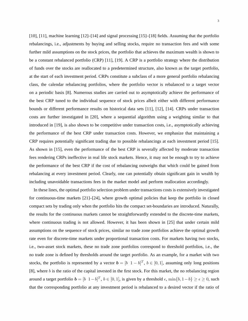
5. outputP ≈ Φk(a,b,Σ) with error estimateE.
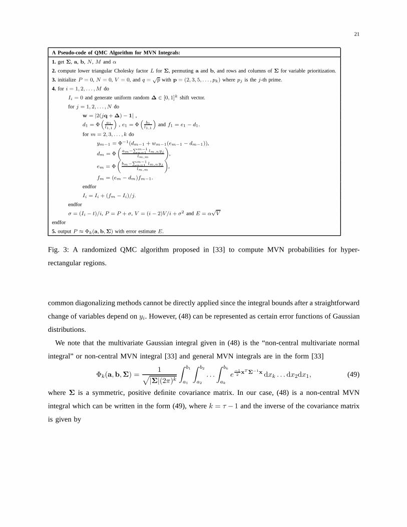
Fig. 3: A randomized QMC algorithm proposed in [33] to compute MVN probabilities for hyper-
rectangular regions.
common diagonalizing methods cannot be directly applied since the integral bounds after a straightforward
change of variables depend onyi. However, (48) can be represented as certain error functions of Gaussian
distributions.
We note that the multivariate Gaussian integral given in (48) is the “non-central multivariate normal
integral” or non-central MVN integral [33] and general MVN integrals are in the form [33]
Φk(a,b,Σ) =1
√
|Σ|(2π)k
∫ b1
a1
∫ b2
a2
. . .
∫ bk
ak
e−1
2xTΣ−1x dxk . . . dx2dx1, (49)
whereΣ is a symmetric, positive definite covariance matrix. In our case, (48) is a non-central MVN
integral which can be written in the form (49), wherek = τ − 1 and the inverse of the covariance matrix
is given by

22
Σ−1 =
2 −1
−1 2 −1
. . . . . . . . .
−1 2 −1
−1 2
which is a symmetric positive definite matrix with|Σ| = 1, the lower bound vector is of the form,
a = [a1, . . . , aτ−1]T ,
a =
κ− θ1 − µ
κ− θ1 − 2µ...
κ− θ1 − (τ − 1)µ
and the upper bound vector is given by,b = [b1, . . . , bτ−1]T ,
b =
κ− θ2 − µ
κ− θ2 − 2µ...
κ− θ2 − (τ − 1)µ
where−kµ terms in the lower and the upper bounds follow from the non-central property of (48). We
emphasize that the MVN integral in (49) cannot be calculatedin a closed form [33] and most of the
results on this integral correspond to either special casesor coarse approximations [33], [34]. Hence,
in this paper, we use the randomized QMC algorithm, providedin Fig. 3 [33] for completeness, to
compute MVN probabilities over hyper rectangular regions.Here, the algorithm uses a periodization and
randomized QMC rule [35], where the output error estimateE in Fig. 3 is the usual Monte Carlo standard
error based onN samples of the randomly shifted QMC rule, and scaled by the confidence factorα.
We observe in our simulations that the algorithm in Fig. 3 produce satisfactory results on the historical
data [15]. We emphasize that different algorithms can be used instead of the Quasi-Monte Carlo (QMC)
algorithm to calculate the multivariable integrals in (48), however, the derivations still hold.
IV. M AXIMUM -L IKELIHOOD ESTIMATION OF PARAMETERS OF THELOG-NORMAL DISTRIBUTION
In this section, we give the MLEs for the mean and variance of the log-normal distribution using the
sequence of price relative vectors, which are used sequentially in the Simulations section to evaluate the
optimal TRPs. Since the investor observes the sequence of price relatives sequentially, he or she needs

23
to estimateµ andσ at each investment period to find the maximizingb andǫ. Without loss of generality
we provide the MLE forx1(t), where the MLE forx2(t) directly follows.
For these derivations, we assume that we observed a sequenceof price relative vectors of lengthN ,
i.e., (x1(1), x1(2), . . ., x1(N)). Note that the sample data need not to belong toN consecutive periods
such that the sequential representation is chosen for ease of presentation. Then, we find the parameters
µ1 andσ21 that maximize the log-likelihood function
lnL(µ1, σ21 |x1(1), x1(2), . . . , x1(N)) = ln f(x1(1), x1(2), . . . , x1(N) |µ1, σ
21) =
N∑
i=1
ln f(x1(i) |µ1, σ1),
wheref(x|µ1, σ21) =
1x√2πσ1
2e− (ln x−µ1)2
2σ12 . The log-likelihood function in (50) can also be written as
lnL(µ1, σ21 |x1(1), x1(2), . . . , x1(N)) =
N∑
i=1
ln1
x1(i)√
2πσ12e− (ln x1(i)−µ1)2
2σ12
=
N∑
i=1
ln1
x1(i)√
2πσ12−
N∑
i=1
(lnx1(i)− µ1)2
2σ12. (50)
We start with maximizing the log-likelihood functionlnL with respect toµ1, i.e., find the estimatorµ1
that satisfies∂ lnL∂µ1
= 0. If we take the partial derivative of the expression in (50) with respect toµ1, then
we obtain
∂ lnL
∂µ1=
N∑
i=1
lnx1(i)− µ1
σ12.
Henceµ1, which satisfies∂L∂µ1= 0, or the ML estimatorµ1 of µ1, can be found as
µ1 =1
N
N∑
i=1
lnx1(i). (51)
To find the ML estimator of the varianceσ21 , we find σ2
1 that satisfies∂ lnL∂σ2
1= 0. Sinceµ1 that satisfies
∂l∂µ1
= 0 in (51) does not depend onσ21 , we can use it in (50). Let us definex1 =
∑Ni=1
lnx1(i)N for
notational clarity. By replacingx1 with µ1 in (51) and taking the partial derivative of the expression with
respect toσ21, we obtain
∂ lnL
∂σ21
= −N
2σ21
+1
2(σ21)
2
N∑
i=1
(lnx1(i)− x1)2.
Hence
σ21 =
1
N
N∑
i=1
(lnx1(i) − x1)2. (52)
24
Following similar steps, the ML estimators forx2(t) yield
µ2 =1
N
N∑
i=1
lnx2(i), (53)
and
σ22 =
1
N
N∑
i=1
(lnx2(i) − x2)2, (54)
wherex2△=
∑Ni=1
lnx2(i)N . Note that the ML estimatorsµ1, σ2
1, µ2 and σ22 are consistent [36], i.e., they
converge to the true values as the size of the data set goes to infinity, i.e.,N → ∞ [31].
V. SIMULATIONS
In this section, we illustrate the performance our algorithm under different scenarios. We first use
TRPs over simulated data of two stocks, where each stock is generated from a log-normal distribution.
We then continue to test the performance over the historical“Ford - MEI Corporation” stock pair chosen
for its volatility [12] from the New York Stock Exchange. As the final set of experiments, we use our
algorithm over the historical data set from [10] and illustrate the average performance. In all these trials,
we compare the performance of our algorithm with portfolio selection strategies from [10], [15], [27].
In the first example, each stock is generated from a log-normal distribution such thatx1(t) ∼ lnN (0.006, 0.05)
andx2(t) ∼ lnN (0.003, 0.05), where the mean and variance values are arbitrarily selected. We observe
that the results do not depend on a particular choice of modelparameters as long as they resemble real
life markets. We simulate the performance over 1100 investment periods. Since the mean and variance
parameters are not known by the investor, we use the ML estimators from Section IV, which are then used
to determine the target portfoliob and the threshold valueǫ. We start by calculating the ML estimators
using the initial 200 samples and find the target portfoliob = [b 1 − b]T and the thresholdǫ that
maximize the expected wealth growth by a brute-force search. Then, we use the correspondingb and
ǫ during the following 200 samples. In similar lines, we calculate and use the optimal TRP for a total
of 900 days, whereb andǫ are estimated over every window of 200 samples and used in thefollowing
window of 200 samples. We choose a window of size 200 samples to get reliable estimates for the
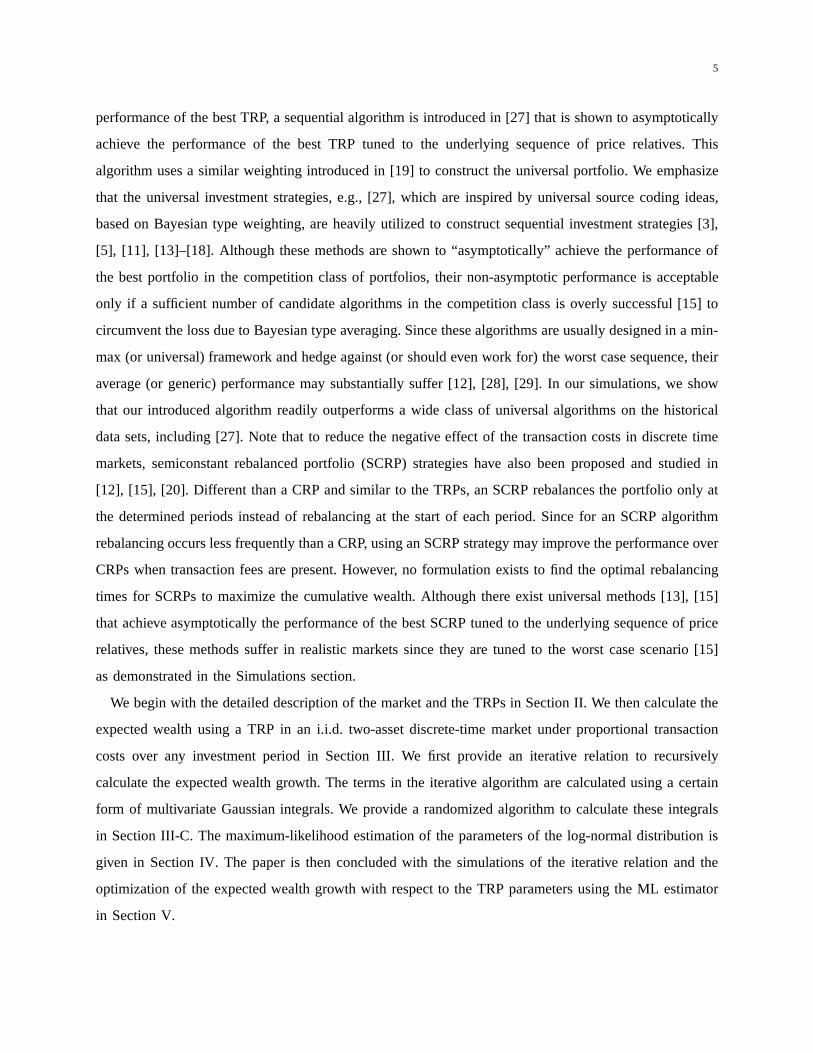
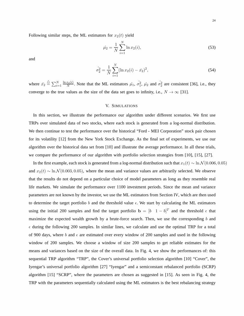
means and variances based on the size of the overall data. In Fig. 4, we show the performances of: this
sequential TRP algorithm “TRP”, the Cover’s universal portfolio selection algorithm [10] “Cover”, the
Iyengar’s universal portfolio algorithm [27] “Iyengar” and a semiconstant rebalanced portfolio (SCRP)
algorithm [15] “SCRP”, where the parameters are chosen as suggested in [15]. As seen in Fig. 4, the
TRP with the parameters sequentially calculated using the ML estimators is the best rebalancing strategy
25
100 200 300 400 500 600 700 800 900
10
20
30
40
50
60
70
80
Investment Period
Wea
lth G
rowth
Performance of TRP under c=0.25 − Log−normally Simulated Market
TRPSCRPIyengarCover
(a)
0 100 200 300 400 500 600 700 800 9000
10
20
30
40
50
60
70
80
90
Investment Period
Wea
lth G
rowth
Performance of TRP under c=0.1 − Log−normally Simulated Market
TRPSCRPIyengarCover
(b)
Fig. 4: Performance of various portfolio investment algorithms ona Log-normally simulated two-stock market. (a)
Wealth growth under hefty transaction cost (c=0.025). (b) Wealth growth under moderate transaction cost (c=0.01).
among the others as expected from our derivations. In Fig. 4aand Fig. 4b, we present results for a mild
transaction costc = 0.01 and a hefty transaction costc = 0.025, respectively, wherec is the fraction paid
in commission for each transaction, i.e.,c = 0.01 is a 1% commission. We observe that the performance
of the TRP algorithm is better than the other algorithms for these transaction costs. However, the relative
gain is larger for the large transaction cost since the TRP approach, with the optimal parameters chosen
as in this paper, can hedge more effectively against the transaction costs.
As the next example, we apply our algorithm to historical data from [10] from the New York Stock
26
500 1000 1500 2000 2500 3000 3500 4000 45000
2
4
6
8
10
12
14
16
18
Investment Period
Wea
lth G
rowth
Performance of TRP under c=0.25 − Ford and MEI Corp.
TRPSCRPIyengarCover
(a)
500 1000 1500 2000 2500 3000 3500 4000 45000
2
4
6
8
10
12
14
16
18
Investment Period
Wea
lth G
rowth
Performance of TRP under c=0.1 − Ford and MEI Corp.
TRPSCRPIyengarCover
(b)
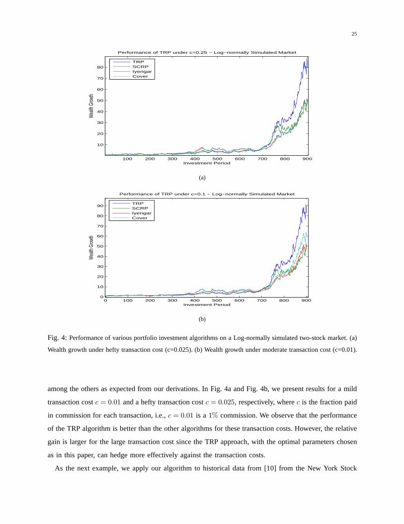
Fig. 5: Performance of various portfolio investment algorithms onFord - MEI Corporation pair. (a) Wealth growth
under hefty transaction cost (c=0.025). (b) Wealth growth under moderate transaction cost (c=0.01).
Exchange collected over a 22-year period. We first apply algorithms on the “Ford - MEI Corporation” pair
as shown in Fig. 5, which are chosen because of their volatility [12]. In Fig. 5, we plot the wealth growth
of: the sequential TRP algorithm with the optimal parameters sequentially calculated, the Cover’s universal
portfolio, the Iyengar’s universal portfolio and the SCRP algorithm with the suggested parameters in [15].
We use the ML estimators to choose the optimal TRP as in the first set of experiments, however, since the
historical data contains 5651 days we use a window of size 1000 days. Hence, the performance results
are shown over 4651 days. As seen from Fig. 5, the proposed TRPalgorithm significantly outperforms
27
500 1000 1500 2000 2500 3000 3500 4000 4500
1
2
3
4
5
6
7
8
9
10
11
TRPSCRPIyengarCover
(a)
0 500 1000 1500 2000 2500 3000 3500 4000 4500
2
4
6
8
10
12
TRPSCRPIyengarCover
(b)
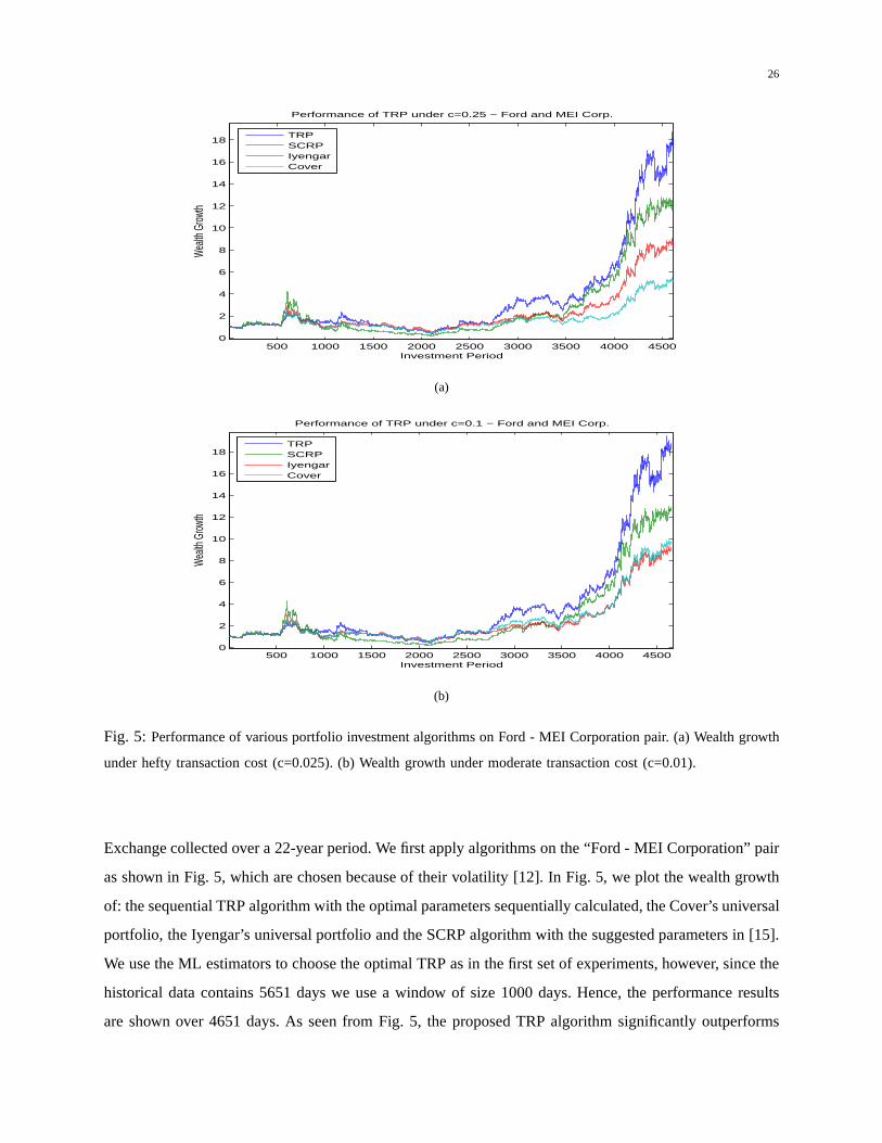
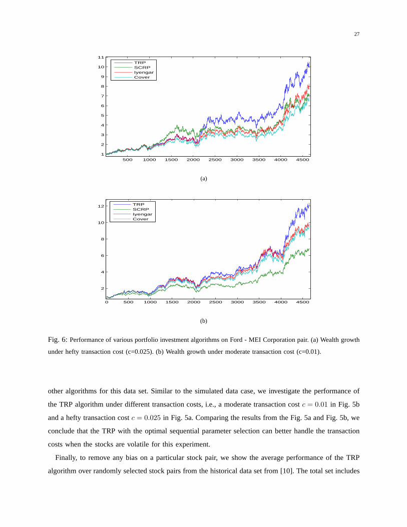
Fig. 6: Performance of various portfolio investment algorithms onFord - MEI Corporation pair. (a) Wealth growth
under hefty transaction cost (c=0.025). (b) Wealth growth under moderate transaction cost (c=0.01).
other algorithms for this data set. Similar to the simulateddata case, we investigate the performance of
the TRP algorithm under different transaction costs, i.e.,a moderate transaction costc = 0.01 in Fig. 5b
and a hefty transaction costc = 0.025 in Fig. 5a. Comparing the results from the Fig. 5a and Fig. 5b,we
conclude that the TRP with the optimal sequential parameterselection can better handle the transaction
costs when the stocks are volatile for this experiment.
Finally, to remove any bias on a particular stock pair, we show the average performance of the TRP
algorithm over randomly selected stock pairs from the historical data set from [10]. The total set includes
28
34 different stocks, where the Iroquois stock is removed dueto its peculiar behavior. We first randomly
select pairs of stocks and invest using: the sequential TRP algorithm with the sequential ML estimators, the
Cover’s universal portfolio algorithm, the Iyengar’s universal portfolio algorithm and the SCRP algorithm.
The sequential selection of the optimal TRP parameters are performed similar to the previous case, i.e.,
we use ML estimators on an investment block of 1000 days and use the calculated optimal TRP in the
next block of 1000 days. For each stock pair, we simulate the performance of the algorithms over 4651
days. In Fig. 6, we present the wealth achieved by these algorithms, where the results are averaged over
10 independent trials. We present the achieved wealth over random sets of stock pairs under a moderate
transaction costc = 0.01 in Fig. 6b and a hefty transaction costc = 0.025 in Fig. 6a. As seen from
the figures, the TRP algorithm with the ML estimators readilyoutperforms the other strategies under
different transaction costs on this historical data set.
VI. CONCLUSION
In this paper, we studied an important financial application, the portfolio selection problem, from
a signal processing perspective. We investigated the portfolio selection problem in i.i.d. discrete time
markets having a finite number of assets, when the market levies proportional transaction fees for both
buying and selling stocks. We introduced algorithms based on threshold rebalanced portfolios that achieve
the maximal growth rate when the sequence of price relativeshave the log-normal distribution from the
well-known Black-Scholes model [8]. Under this setup, we provide an iterative relation that efficiently
and recursively calculates the expected wealth in any i.i.d. market over any investment period. The terms
in this recursion are evaluated by a certain multivariate Gaussian integral. We then use a randomized
algorithm to calculate the given integral and obtain the expected growth. This expected growth is then
optimized by a brute force method to yield the optimal targetportfolio and the threshold to maximize the
expected wealth over any investment period. We also providea maximum-likelihood estimator to estimate
the parameters of the log-normal distribution from the sequence of price relative vectors. As predicted
from our derivations, we significantly improve the achievedwealth over portfolio selection algorithms
from the literature on the historical data set from [10].
REFERENCES
[1] IEEE Journal of Selected Topics in Signal Processing, “Special issue on signal processing methods in finance and electronic
trading,” http://www.signalprocessingsociety.org/uploads/specialissuesdeadlines/spfinance.pdf.
[2] IEEE Signal Processing Magazine, “Special issue on signal processing for financial applications,”
http://www.signalprocessingsociety.org/uploads/Publications/SPM/financialapps.pdf.

29
[3] A. Bean and A. C. Singer, “Factor graphs for universal portfolios,” in Proceedings of the Forty-Third Asilomar Conference
on Signals, Systems and Computers, 2009, pp. 1375–1379.
[4] M. U. Torun, A. N. Akansu, and M. Avellaneda, “Portfolio risk in multiple frequencies,”IEEE Signal Processing Magazine,
vol. 28, no. 5, pp. 61–71, Sep 2011.
[5] A. Bean and A. C. Singer, “Universal switching and side information portfolios under transaction costs using factor
graphs,” inProceedings of the ICASSP, 2010, pp. 1986–1989.
[6] A. Bean and A. C. Singer, “Portfolio selection via constrained stochastic gradients,” inProceedings of the SSP, 2011, pp.
37–40.
[7] M. U. Torun and A. N. Akansu, “On basic price model and volatility in multiple frequencies,” inProceedings of the SSP,
June 2011, pp. 45–48.
[8] D. Luenberger,Investment Science, Oxford University Press, 1998.
[9] H. Markowitz, “Portfolio selection,”Journal of Finance, vol. 7, no. 1, pp. 77–91, 1952.
[10] T. Cover, “Universal portfolios,”Mathematical Finance, vol. 1, pp. 1–29, January 1991.
[11] T. Cover and E. Ordentlich, “Universal portfolios withside-information,” IEEE Transactions on Information Theory, vol.
42, no. 2, pp. 348–363, 1996.
[12] D. P. Helmbold, R. E. Schapire, Y. Singer, and M. K. Warmuth, “Online portfolio selection using multiplicative updates,”
Mathematical Finance, vol. 8, pp. 325–347, 1998.
[13] Y. Singer, “Swithcing portfolios,” inProc. of Conf. on Uncertainty in AI, 1998, pp. 1498–1519.
[14] V. Vovk and C. Watkins, “Universal portfolio selection,” in Proceedings of the COLT, 1998, pp. 12–23.
[15] S. S. Kozat and A. C. Singer, “Universal semiconstant rebalanced portfolios,”Mathematical Finance, vol. 21, no. 2, pp.
293–311, 2011.
[16] S. S. Kozat and A. C. Singer, “Switching strategies for sequential decision problems with multiplicative loss withapplication
to portfolios,” IEEE Transactions on Signal Processing, vol. 57, no. 6, pp. 2192–2208, 2009.
[17] S. S. Kozat and A. C. Singer, “Universal switching portfolios under transaction costs,” inProceedings of the ICASSP,
2008, pp. 5404–5407.
[18] S. S. Kozat, A. C. Singer, and A. J. Bean, “A tree-weighting approach to sequential decision problems with multiplicative
loss,” Signal Processing, vol. 92, no. 4, pp. 890–905, 2011.
[19] T. M. Cover and C. A. Thomas,Elements of Information Theory, Wiley Series, 1991.
[20] A. Blum and A. Kalai, “Universal portfolios with and without transaction costs,”Machine Learning, vol. 35, pp. 193–205,
1999.
[21] M. H. A. Davis and A. R. Norman, “Portfolio selection with transaction costs,”Mathematics of Operations Research, vol.
15, pp. 676713, 1990.
[22] M. Taksar, M. Klass, and D. Assaf, “A diffusion model foroptimal portfolio selection in the presence of brokerage fees,”
Mathematics of Operations Research, vol. 13, pp. 277–294, 1988.
[23] A. J. Morton and S. R. Pliska, “Optimal portfolio manangement with transaction costs,”Mathematical Finance, vol. 5,
pp. 337–356, 1995.
[24] M. J. P. Magill and G. M. Constantinides, “Portfolio selection with transactions costs,”Journal of Economic Theory, vol.
13, no. 2, pp. 245–263, 1976.
[25] G. Iyengar, “Discrete time growth optimal investment with costs,” http://www.ieor.columbia.edu/ gi10/Papers/stochastic.pdf.

30
[26] G. Iyengar and T. Cover, “Growths optimal investment inhorse race markets with costs,”IEEE Transactions on Information
Theory, vol. 46, pp. 2675–2683, 2000.
[27] G. Iyengar, “Universal investment in markets with transaction costs,”Mathematical Finance, vol. 15, no. 2, pp. 359–371,
2005.
[28] A. Borodin, R. El-Yaniv, and V. Govan, “Can we learn to beat the best stock,”Journal of Artificial Intelligence Research,
vol. 21, pp. 579–594, 2004.
[29] J. E. Cross and A. R. Barron, “Efficient universal portfolios for past dependent target classes,”Mathematical Finance,
vol. 13, no. 2, pp. 245–276, 2003.
[30] Z. Bodie, A. Kane, and A. Marcus,Investments, McGraw-Hill/Irwin, 2004.
[31] H. Stark and J. W. Woods,Probability And Random Processes With Applications To Signal Processing, Prentice-Hall,
2001.
[32] N. H. Timm, Applied Multivariate Analysis, Springer, 2002.
[33] A. Genz and F. Bretz,Computation of Multivariate Normal and t Probabilities, Springer, 2009.
[34] I. F. Blake and W. C. Lindsey, “Level-crossing problemsfor random processes,”IEEE Transactions on Information Theory,
vol. 19, no. 3, May 1973.
[35] R. Richtmyer, “The evaluation of definite integrals andquasi-monte carlo method based on the properties of algebraic
numbers,” Los Alamos Scientific Laboratory, Los Alamos, NM.
[36] D. Ruppert,Statistics and Data Analysis for Financial Engineering, Springer, 2010.


