
12/01 - 1
Target Precision Determination and Integrated
NavigationBy
Professors Dominick Andrisani and James Bethel,
and Ph.D. students Aaron Braun, Ade Mulyana and Takayuki Hoshizaki
Purdue University, West Lafayette, IN 47907-1282
[email protected] 755-494-5135
[email protected] 755-494-6719
NIMA Meetings
December 11-12, 2001
http://bridge.ecn.purdue.edu/~uav

12/01 - 2
To provide an overview of the results of the Purdue Motion Imagery Group which is studying precision location of ground targets from a UAV. (This work started January ‘01).
To suggest that integrated navigators have to be re-optimizedin in regards to allowable errors in position and orientation of the aircraft for the problem of locating ground targets.
To build a case for a new class of aircraft navigators that use imagery to improve aircraft navigation accuracy.
To build a case for a new class of target locators that integrate aircraft navigation and target imagery to improve accuracy of aircraft location and target location.
Purposes of this talk

12/01 - 3
This summary talk will be short on mathematics, procedural details, and numerical results.
This summary talk will be big on ideas and concepts thatwe have identified as being important in improvingthe accuracy of target location from an UAV.
Our final report will be available through contract sponsorDave Rogers in early April.
Papers documenting the details of our work and work-in-progress can be found at http://bridge.ecn.purdue.edu/~uav
(This site is password protected. Contact Dave for password.)
Note to the Audience

12/01 - 4
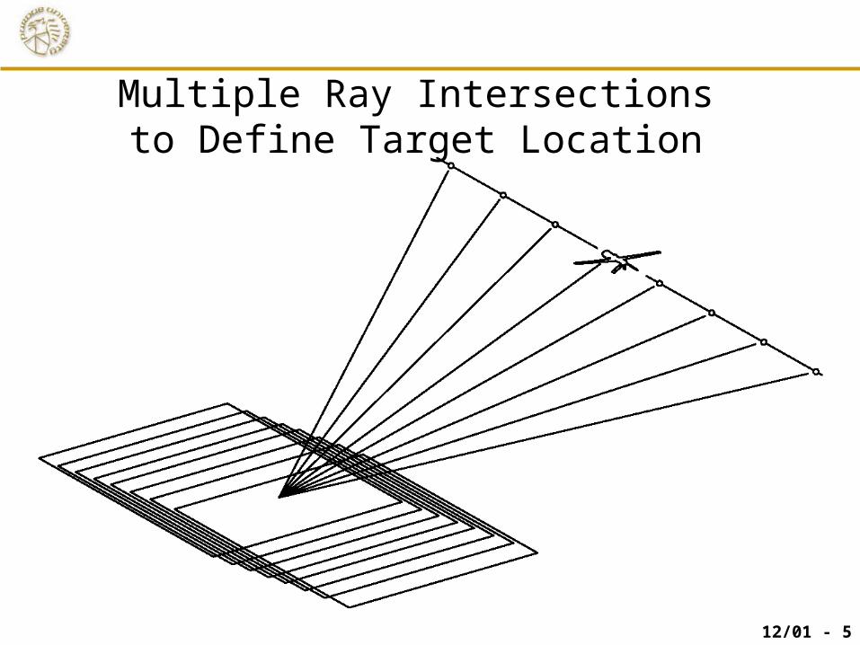
To study location of both target and aircraft using motion Imagery with multiple ray intersections, inertial sensors, and the GPS system, and to do this with as few simplifying assumptions as possible.
To determine which sources of error contribute most toerrors in locating a ground target.
To determine an error budget that will guarantee a cep90% of 10 feet.
Objectives of the Purdue Motion Imagery Group
12/01 - 5
Multiple Ray Intersections to Define Target Location
12/01 - 6
Aircraft Motion
Aircraft Model
Trajectory Input
Time Input
Turbulence Input
Errors
GPS
Satellite Constellation
Processing Mode
AntennasNumber, Location
Errors
INS
Position, Attitude, Rates Position, Attitude, Rates
Filter
Aircraft Position & Attitude Estimate and Uncertainty
Transformation to Sensor Position, Attitude, and Uncertainty
Errors
ErrorsSensor Parameters
Image AcquisitionParameters
Site Model
Imaging System
Target CoordinatesUncertainty, CE90
Graphic Animation
Multi-ImageIntersection
Synthetic Image GenerationErrors
Target Tracking
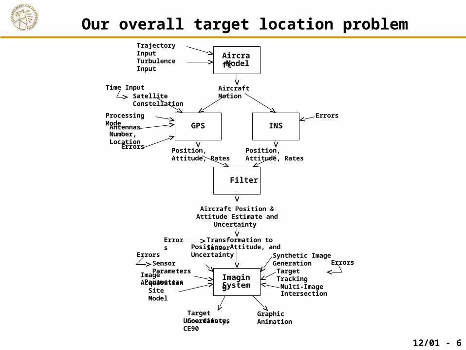
Our overall target location problem

12/01 - 7
Aircraft Motion
Aircraft Model
Trajectory Input
Time Input
Turbulence Input
Errors
GPS
Satellite Constellation
Processing Mode
AntennasNumber, Location
Errors
INS
Position, Attitude, Rates Position, Attitude, Rates
Filter
Aircraft Position & Attitude Estimate and Uncertainty
Transformation to Sensor Position, Attitude, and Uncertainty
Errors
ErrorsSensor Parameters
Image AcquisitionParameters
Site Model
Imaging System
Target Coordinates
Uncertainty, CE90
Graphic Animation
Multi-ImageIntersection
Synthetic Image GenerationErrors
Target Tracking
Given covariance ofzero mean errors
Find target position covariance (cep90) using linear methods
Problem: Errors are not alwayszero mean
Covariance Analysis

12/01 - 8
See References by Aaron Braun
•Rigorous sensor modeling is important in determining target location.•Aircraft orientation and aircraft position accuracy are bothimportant in target location accuracy. •The relative importance of various error sources to the CEP90 is being determined.
Covariance Analysis
See References by Professor James Bethel Sometimes errors are not zero mean but biased. The best example of this is in GPS positioning. Quoted GPSaccuracy reflects the sum of the bias and randomcomponents. Biased aircraft positioning will lead to biasedtarget positioning. Covariance analysis will not show this fact.
12/01 - 9
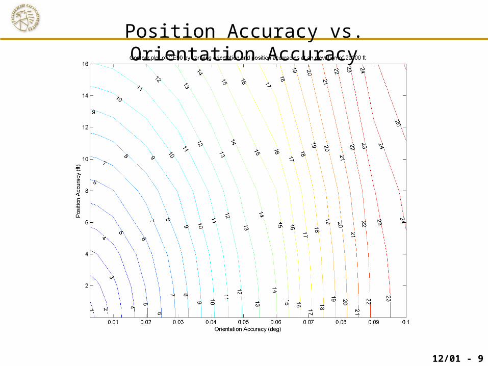
Position Accuracy vs. Orientation Accuracy

12/01 - 10
Stand-Alone Target Precision Calculator
12/01 - 11
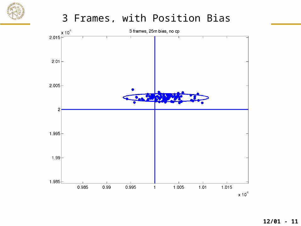
3 Frames, with Position Bias

12/01 - 12
Aircraft Motion
Aircraft Model
Trajectory Input
Time Input
Turbulence Input
Errors
GPS
Satellite Constellation
Processing Mode
AntennasNumber, Location
Errors
INS
Position, Attitude, Rates Position, Attitude, Rates
Filter
Aircraft Position & Attitude Estimate and Uncertainty
Transformation to Sensor Position, Attitude, and Uncertainty
Errors
ErrorsSensor Parameters
Image AcquisitionParameters
Site Model
Imaging System
Target CoordinatesUncertainty, CE90
Graphic Animation
Multi-ImageIntersection
Synthetic Image GenerationErrors
Target Tracking
Today’s Integrated Inertial Navigator (Inertial + GPS)

12/01 - 13
Status of our work on an Integrated Inertial Navigator
Ade Mulyana and Taka Hoshizaki have completed the development of an integrated navigator of this form.
Results show that improving the GPS subsystem produces a significant improvement in aircraft position accuracy.
Results also show that improving the inertial navigation subsystem produces a significant improvement in aircraft orientation accuracy.
Since both aircraft position and orientation are importantin targeting, careful re-optimization of the INS and GPS systems is required for the ground targeting scenario. Our error budget will help in this re-optimization.
See References by Mulyana and Hoshizaki

12/01 - 14
Local Frame Position Errors: (true) – (estimated)
0 50 100 150 200 250 300 350 400-5
0
5
10Local Frame Position Errors
dx (
m)
0 50 100 150 200 250 300 350 400-5
0
5
10
dy (
m)
gIgGwIgGwIwGgIwG
0 50 100 150 200 250 300 350 400-10
-5
0
5
dz (
m)
time (s)0 400 (sec)
dx (m)
dy (m)
dz (m)
blue red (:) black (-.) green (--)INS good worse worse goodGPS good good worse worse
• GPS performance directly affects position errors
200~300s covariance and nominal trajectory data are passed to imagery analysis

12/01 - 15
0 50 100 150 200 250 300 350 400-2
-1
0
1x 10
-3 Euler Angle Errors
dE1
(rad
)
0 50 100 150 200 250 300 350 400-15
-10
-5
0
5x 10
-4
dE2
(rad
)
gIgGwIgGwIwGgIwG
0 50 100 150 200 250 300 350 400-3
-2
-1
0x 10
-3
dE3
(rad
)
time (s)
0 400 (sec)
droll (rad)
dpitch (rad)
dyaw (rad)
Local Frame Euler Angle Errors: (true) – (estimated)
blue red (:) black (-.) green (--)INS good worse worse goodGPS good good worse worse
• INS accuracy helps orientation accuracy

12/01 - 16
Aircraft Motion
Aircraft Model
Trajectory Input
Time Input
Turbulence Input
Errors
GPS
Satellite Constellation
Processing Mode
AntennasNumber, Location
Errors
INS
Position, Attitude, Rates Position, Attitude, Rates
Filter
Aircraft Position & Attitude Estimate and Uncertainty
Transformation to Sensor Position, Attitude, and Uncertainty
Errors
ErrorsSensor Parameters
Image AcquisitionParameters
Site Model
Imaging System
Target Coordinates
Uncertainty, CE90
Graphic Animation
Multi-ImageIntersection
Synthetic Image GenerationErrors
Target Tracking
Do all this simultaneouslyfor improved accuracy inaircraft positioning.
The targetsmay include oneor more known control points.
Known control points improveaircraft accuracy.
Proposed Imaging Navigator (Inertial+GPS+ Imagery)

12/01 - 17
Status of our work on the Imaging Navigator
A fully integrated nonlinear Imaging Navigator will be developed under a subsequent contract.
Preliminary analysis by Andrisani using greatly simplified models and linear analysis are encouraging.
Flying over known control points improve aircraft position accuracy. This is a standard INS update technique.
Flying over stationary objects on the ground should minimize the effects of velocity biases and rate gyro biases in the inertial navigator. This should improve aircraft position and orientation accuracy.

12/01 - 18
Aircraft Motion
Aircraft Model
Trajectory Input
Time Input
Turbulence Input
Errors
GPS
Satellite Constellation
Processing Mode
AntennasNumber, Location
Errors
INS
Position, Attitude, Rates Position, Attitude, Rates
Filter
Aircraft Position & Attitude Estimate and Uncertainty
Transformation to Sensor Position, Attitude, and Uncertainty
Errors
ErrorsSensor Parameters
Image AcquisitionParameters
Site Model
Imaging System
Target Coordinates
Uncertainty, CE90
Graphic Animation
Multi-ImageIntersection
Synthetic Image GenerationErrors
Target Tracking
Do all this simultaneouslyfor improved accuracy intarget positioning
The targetsmay include oneor more known control points.
Known control points improvetarget accuracy.
Proposed Integrated Target Locator (Inertial+GPS+ Imagery)

12/01 - 19
Status of our work on the Integrated Target Locator
A nonlinear Integrated Target Locator will be developed under a subsequent contract.
Preliminary analysis by Andrisani using greatly simplified models and linear analysis is encouraging.
Flying over known control points improves target position accuracy.
Flying over stationary objects on the ground should minimize the effects of velocity biases and rate gyro biases in the inertial navigator. This should improve target position accuracy.

12/01 - 20
Hypothesis:
Given a combined estimator of aircraft position and target position capable of imaging on a unknown target and a known control point.
If a control point enters the field of view of the imagesystem, the accuracy of simultaneous estimation of aircraft position and unknown target position will be significantly improved.
Simplified Integrated Target Locator

12/01 - 21
Use a linear low-order simulation of a simplified linear aircraft model,
Use a simple linear estimator to gain insight into the problem with a minimum of complexity.
A control point of known location will enter the field of view of the image processor only during the time from 80-100 seconds.
Technical Approach

12/01 - 22
0Unknown Target always visible
Initial aircraft position time=0 sec Final aircraft position time=200 sec
-10,000 10,000
Range Meas., R (ft)
Position (ft)
Image Coord. Meas. x (micron)
Position MeasXaircraft (ft) Focal Plane (f=150 mm)
Camera always looks down.
20,000Nominal speed=100 ft/sec
Data every .1 sec., i.e., every 10 ft
Control pointKnown locationVisible only fromtime=80-100 seconds.
Linear Simulation: Fly over trajectory

12/01 - 23
Aircraft position = 1 feet Image coordinate = 7.5 microns
Range = 1 feet
Nominal Measurement Noise in the Simulation
12/01 - 24
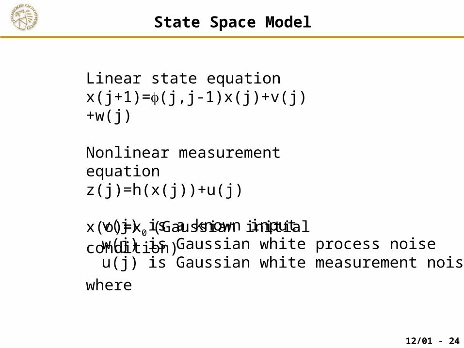
Linear state equationx(j+1)=(j,j-1)x(j)+v(j)+w(j)
Nonlinear measurement equationz(j)=h(x(j))+u(j)
x(o)=x0 (Gaussian initial condition)
where
v(j) is a known inputw(j) is Gaussian white process noiseu(j) is Gaussian white measurement noise
State Space Model

12/01 - 25
Initialize 0ˆ)0|0(ˆ ,
0)0|0( xxPP
Predict one step
Measurement update)1()1|1(ˆ)1,()1|(ˆ
)1()1,()1|1()1,()1|(
jvjjxjjjjx
jQjjjjPjjjjP T
)(~)()1|(ˆ)|(ˆ
FilterKalman theof Residuals ))1|(ˆ()()(~
)1|()]()([)|(
)1|()()1|()(
)()()1|()()1|(1
jzjKjjxjjx
jjxhjzjz
jjPjHjKIjjP
jjPjHjjPjK
jRjHjjPjHjjP
ZT
TZ
The Kalman Filter State Estimator

12/01 - 26
Estimation results for different measurement noises
Measurement Noise (sigma values)units Run1 Run2 Run3 Run4 Run5 Run6
aircraft position feet 100 10 1 0.1 1 1image coord micron 7.5 7.5 7.5 7.5 75 750range feet 1 1 1 1 10 100
Final position estimates (sigma values)units
aircraft position feet 0.78 0.77 0.6 0.099 0.78 0.78target position feet 0.095 0.088 0.03 0.021 0.21 0.22
** **** These runs were greatly effected by the appearance of the known control point during 80-100 seconds.
Tabulated Results

12/01 - 27
0 20 40 60 80 100 120 140 160 180 200-500
0
500
Res
(XL)
ft + and - 2sigma bounds
Run #1: SigmaR=100 ft,7.5 micron,1 ft
0 20 40 60 80 100 120 140 160 180 200-50
0
50
Res
(x1)
mro
n
0 20 40 60 80 100 120 140 160 180 200-5
0
5
Res
(R1)
ft
0 20 40 60 80 100 120 140 160 180 200-100
0
100
Res
(x2)
mro
n
0 20 40 60 80 100 120 140 160 180 200-5
0
5
Res
(R2)
ft
time (sec)
No measurement here No measurement here
No measurement here No measurement here
Residuals of the Kalman Filter, aircraft =100 ft
AircraftPositionresidual (ft)
Target1PositionError (ft)
Target2PositionError (ft)

12/01 - 28
0 20 40 60 80 100 120 140 160 180 200-100
0
100
Act
err
(XL)
ft Act Err = Xhat-Xexact. + and - 2sigma theoretical bounds
Std1(last half)= 0.79861 SigmaTheoryFinal1= 0.77584
Run #1: SigmaR=100 ft,7.5 micron,1 ft
0 20 40 60 80 100 120 140 160 180 200-100
0
100
Act
err
(XP
1)ft
Std2(last half)= 0.00080613 SigmaTheoryFinal2= 0.095274
0 20 40 60 80 100 120 140 160 180 200-1
0
1
Act
err
(XP
2)ft
time (sec)
Std3(last half)= 0 SigmaTheoryFinal3= 0
Major impact of control point here
Major impact of control point here
Estimated State – Actual State , aircraft =100 ft
AircraftPositionError (ft)
Target1PositionError (ft)
Target2PositionError (ft)

12/01 - 29
60 70 80 90 100 110 120-10
0
10
20
Act
err
(XL)
ft Act Err = Xhat-Xexact. + and - 2sigma theoretical bounds
Run #1: SigmaR=100 ft,7.5 micron,1 ft
60 70 80 90 100 110 120-10
0
10
Act
err
(XP
1)ft
60 70 80 90 100 110 120-1
0
1
Act
err
(XP
2)ft
time (sec)
Major impact of control point here
Major impact of control point here
Expanded time scale for Estimated state -Actual state
AircraftPositionError (ft)
Target1PositionError (ft)
Target2PositionError (ft)

12/01 - 30
0 20 40 60 80 100 120 140 160 180 200-10
0
10
Act
err
(XL)
ft Act Err = Xhat-Xexact. + and - 2sigma theoretical bounds
Std1(last half)= 0.79504 SigmaTheoryFinal1= 0.77233
Run #2: SigmaR=10 ft,7.5 micron,1 ft
0 20 40 60 80 100 120 140 160 180 200-10
0
10
Act
err
(XP
1)ft
Std2(last half)= 0.0056979 SigmaTheoryFinal2= 0.088282
0 20 40 60 80 100 120 140 160 180 200-1
0
1
Act
err
(XP
2)ft
time (sec)
Std3(last half)= 0 SigmaTheoryFinal3= 0
Estimated State – Actual State, aircraft =10 ft
AircraftPositionError (ft)
Target1PositionError (ft)
Target2PositionError (ft)

12/01 - 31
60 70 80 90 100 110 120-5
0
5
Act
err
(XL)
ft Act Err = Xhat-Xexact. + and - 2sigma theoretical bounds
Run #2: SigmaR=10 ft,7.5 micron,1 ft
60 70 80 90 100 110 120-1
0
1
Act
err
(XP
1)ft
60 70 80 90 100 110 120-1
0
1
Act
err
(XP
2)ft
time (sec)
Major impact of control point here
Expanded time scale, aircraft =10 ft
AircraftPositionError (ft)
Target1PositionError (ft)
Target2PositionError (ft)

12/01 - 32
0 20 40 60 80 100 120 140 160 180 200-4
-2
0
2
Act
err
(XL)
ft Act Err = Xhat-Xexact. + and - 2sigma theoretical bounds
Std1(last half)= 0.60885 SigmaTheoryFinal1= 0.59831
Run #3: SigmaR=1 ft,7.5 micron,1 ft
0 20 40 60 80 100 120 140 160 180 200-1
0
1
Act
err
(XP
1)ft
Std2(last half)= 0.0060581 SigmaTheoryFinal2= 0.030299
0 20 40 60 80 100 120 140 160 180 200-1
0
1
Act
err
(XP
2)ft
time (sec)
Std3(last half)= 0 SigmaTheoryFinal3= 0
No impact of control point
Little impact of control point here
Estimated State – Actual State, aircraft =1 ft
AircraftPositionError (ft)
Target1PositionError (ft)
Target2PositionError (ft)

12/01 - 33
60 70 80 90 100 110 120-4
-2
0
2
Act
err
(XL)
ft Act Err = Xhat-Xexact. + and - 2sigma theoretical bounds
Run #3: SigmaR=1 ft,7.5 micron,1 ft
60 70 80 90 100 110 120-0.2
0
0.2
Act
err
(XP
1)ft
60 70 80 90 100 110 120-1
0
1
Act
err
(XP
2)ft
time (sec)
Littler impact of control point here
Expanded time scale, aircraft =1 ft
AircraftPositionError (ft)
Target1PositionError (ft)
Target2PositionError (ft)

12/01 - 34
0 20 40 60 80 100 120 140 160 180 200-5
0
5
Act
err
(XL)
ft Act Err = Xhat-Xexact. + and - 2sigma theoretical bounds
Std1(last half)= 0.78796 SigmaTheoryFinal1= 0.78316
Run #5: SigmaR=1 ft,75 micron,10 ft
0 20 40 60 80 100 120 140 160 180 200-10
0
10
Act
err
(XP
1)ft
Std2(last half)= 0.055301 SigmaTheoryFinal2= 0.21331
0 20 40 60 80 100 120 140 160 180 200-1
0
1
Act
err
(XP
2)ft
time (sec)
Std3(last half)= 0 SigmaTheoryFinal3= 0
No impact of control point here
Estimated State – Actual State, Range=10 ft.
AircraftPositionError (ft)
Target1PositionError (ft)
Target2PositionError (ft)

12/01 - 35
60 70 80 90 100 110 120-5
0
5
Act
err
(XL)
ft Act Err = Xhat-Xexact. + and - 2sigma theoretical bounds
Run #5: SigmaR=1 ft,75 micron,10 ft
60 70 80 90 100 110 120-1
0
1
Act
err
(XP
1)ft
60 70 80 90 100 110 120-1
0
1
Act
err
(XP
2)ft
time (sec)
No impact of control point here
Expanded time scale, Range=10 ft.
AircraftPositionError (ft)
Target1PositionError (ft)
Target2PositionError (ft)
12/01 - 36
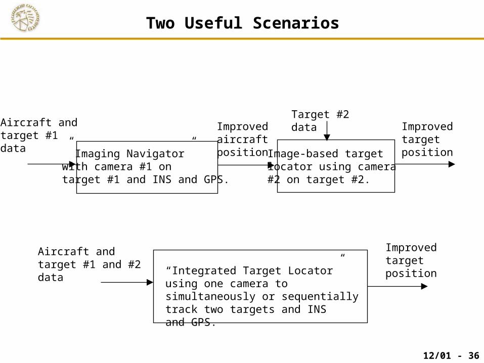
” Imaging Navigator” with camera #1 on target #1 and INS and GPS.
Image-based targetlocator using camera#2 on target #2.
Improvedaircraft position
Improvedtarget position
Aircraft and target #1 and #2 data
“Integrated Target Locator”using one camera to simultaneously or sequentially track two targets and INSand GPS.
Aircraft and target #1 data
Improvedtarget position
Target #2 data
Two Useful Scenarios

12/01 - 37
1. Both aircraft position and orientation accuracy strongly effect the accuracy of target location.
2. Accuracy specifications for position and orientation in integrated inertial navigators should be re-optimized for the problem of achieving desired accuracy in target location. Our error budget to achieve 10 ft cep90% should help in this re-optimization.
3. Regarding our proposed “Integrated Target Locator,” when the measurement noise on aircraft position is large (aircraft>>1 ft), the sighting of a known control point significantly improves the aircraft position accuracy AND the unknown target position accuracy. This suggests a that flying over control points is tactically useful!
4. A dramatic improvement of aircraft position estimation suggests a new type of navigator, the “Imaging Navigator” should be developed. This navigator would integrate INS, GPS, and image processor looking at known or unknown objects on the ground. One or two cameras might be used.
Conclusions

12/01 - 38
Presented at the The Motion Imagery Geolocation Workshop, SAIC Signal Hill Complex,
10/31/01 1. Dominick Andrisani, Simultaneous Estimation of Aircraft and Target Position With a Control Point
2. Ade Mulyana, Takayuki Hoshizaki, Simulation of Tightly Coupled INS/GPS Navigator
3. James Bethel, Error Propagation in Photogrammetric Geopositioning
4. Aaron Braun, Estimation Models and Precision of Target Determination
References
Presented at the The Motion Imagery Geopositioning Review and Workshop, Purdue University, 24/25 July, 2001
1. Dominick Andrisani, Simultaneous Estimation of Aircraft and Target Position
2. Jim Bethel, Motion Imagery Modeling Study Overview
3. Jim Bethel, Data Hiding in Imagery
4. Aaron Braun, Estimation and Target Accuracy
5. Takayuki Hoshizaki and Dominick Andrisani, Aircraft Simulation Study Including Inertial Navigation System (INS) Model with Errors
6. Ade Mulyana, Platform Position Accuracy from GPS

12/01 - 39
1. B.H. Hafskjold, B. Jalving, P.E. Hagen, K. Grade, Integrated Camera-Based Navigation, Journal of Navigation, Volume 53, No. 2, pp. 237-245.2. Daniel J. Biezad, Integrated Navigation and Guidance Systems, AIAA Education Series, 1999.3. D.H. Titterton and J.L. Weston, Strapdown Inertial Navigation Technology, Peter Peregrinus, Ltd., 1997.4. A. Lawrence, Modern Inertial Technology, Springer, 1998.5. B. Stietler and H. Winter, Gyroscopic Instruments and Their Application to Flight Testing, AGARDograph No. 160, Vol. 15,1982.6. A.K. Brown, High Accuracy Targeting Using a GPS-Aided Inertial Measurement Unit, ION 54th Annual Meeting, June 1998, Denver, CO.
Related Literature

12/01 - 40
GPS Receiver
IMU Nav
Structure of Simulation
Tightly Coupled INS/GPS
Position
Velocity
Orientation
Covariance
UAV
Kalman Filter
+
-
INS
Bias Correction
Position, Velocity, Orientation and Covariance correction

12/01 - 41
Simplified IMU Model
δxxx~ where
δx = Bias + White Noise
: Sensor Output
: Sensor Input
Bias : Markov Process, tc=60s
for all
x~
x
zyx
zyx
,,a,a,a
xAccelerometer Outputs
Rate Gyro Outputs

12/01 - 42
GPS Receiver Model
dt
dρΔ
dt
tdc
dt
dρ
dt
dρ
ΔρΔtc2z)(Z2y)(Y2x)(Xρ
GPS
GPS
: Platform Position
dt
d
dt
tdc
tcz,y,xZ,Y,X
where
: Satellite Position
: Pseudorange equvalent
Clock Bias (Random Walk)
: Pseudorange rate equivalent
Clock Drift (Random Walk): Normally Distributed Random Number
: Normally Distributed Random Number
Pseudorange
Pseudorange Rate

12/01 - 43
Kalman Filter: Error Dynamics
]dt
tdct,c
,B,B,B,B,B,B
δh,δλ,δφ,,δv,δv,δv
δγ,δβ,δα,[δx
dt
d
azayax
ωzωyωx
DEN
GvδxFδx
Orientation Angle Errors
17 States Kalman Filter
Velocity Errors
Position Errors
Gyro Biases
Accelerometer Biases
Clock Bias and Drift
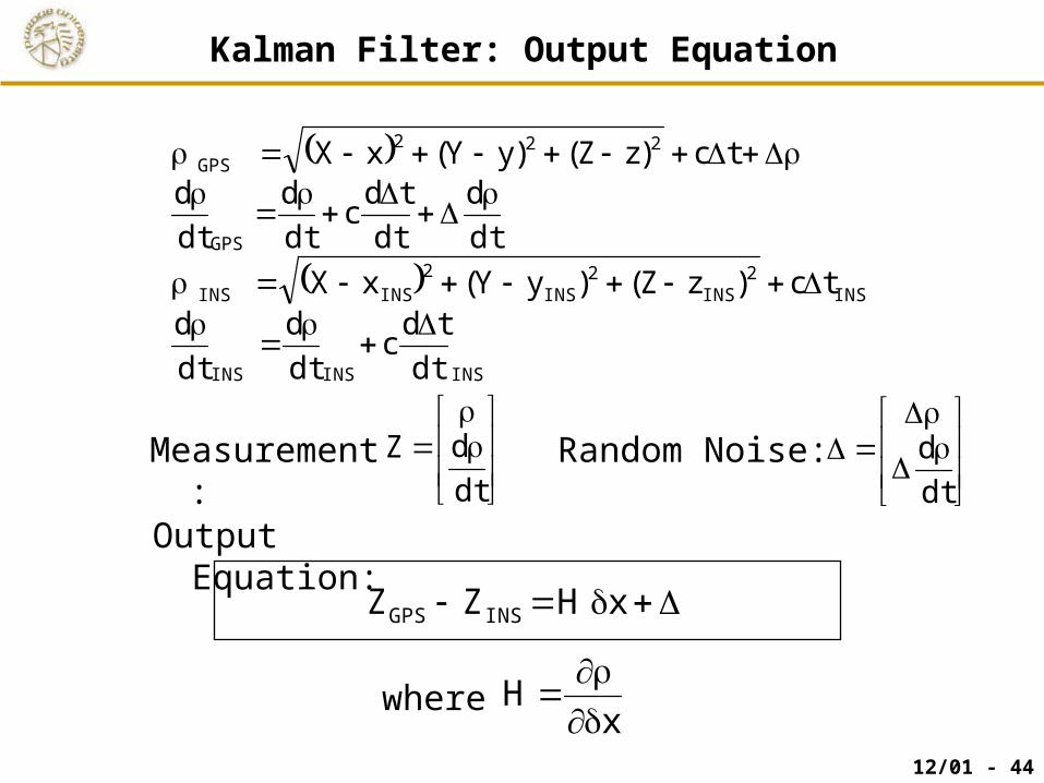
12/01 - 44
Kalman Filter: Output Equation
INSINSINS
INS2
INS2
INS2
INSINS
GPS
222GPS
dt
tdc
dt
d
dt
dtc)zZ()yY(xX
dt
d
dt
tdc
dt
d
dt
dtc)zZ()yY(xX
Measurement:
dt
dZ Random Noise:
dt
d
xHZZ INSGPS
Output Equation:
xH
where
12/01 - 45
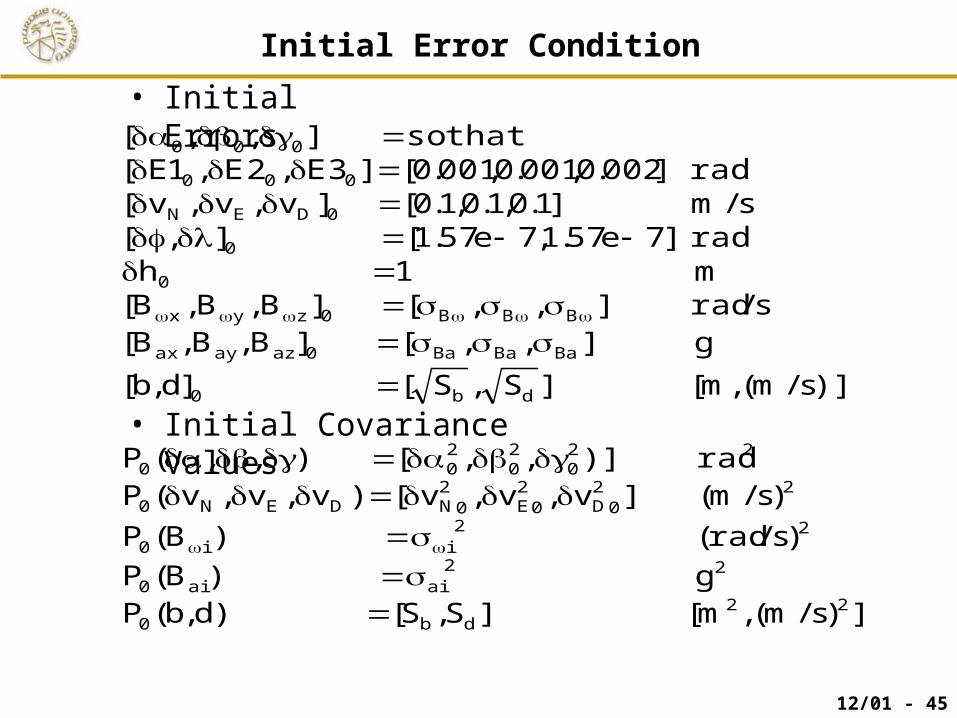
Initial Error Condition
])s/m(,m[]S,S[)d,b(Pg)B(P
)s/rad()B(P
)s/m(]v,v,v[)v,v,v(Prad)],,[),,(P
)]s/m(,m[]S,S[]d,b[
g],,[]B,B,B[s/rad],,[]B,B,B[
m1hrad]7e57.1,7e57.1[],[
s/m]1.0,1.0,1.0[]v,v,v[rad]002.0,001.0,001.0[]3E,2E,1E[
thatso],,[
22db0
22aiai0
22ii0
20
2D0
2E0
2NDEN0
220
20
200
db0
BaBaBa0azayax
BBB0zyx
0
0
0DEN
000
000
• Initial Errors
• Initial Covariance Values

12/01 - 46
Error Source Specifications
r)deg/sqrt(h0.070.0015Ndeg/hr 0.35 0.003
)Hz(sqrt/g505Ng5025
B
a
Ba
INS
AccelerometersBias White Noise (sqrt(PSD))
Bias White Noise (sqrt(PSD))
Notation LN-100G LN-200IMU Units
Rate Gyros
(good) (worse)
• 2 levels of INS are used for Simulation
)(
)(
(deg/hr/sqrt(Hz))

12/01 - 47
Error Source Specifications
GPS
GPS Receiver Notation Receiver 1 Receiver 2 Units
Pseudorange 6.6 33.3 m
Pseudorange Rate 0.05 0.5 m/s
ClockBias White Noise(PSD) 0.009 0.009
ClockDrift White Noise(PSD) 0.0355 0.0355
r
rr
bS
dS
2m2)s/m(
)()(
(good) (worse)
• 2 levels of GPS Receivers are used for Simulation
12/01 - 48
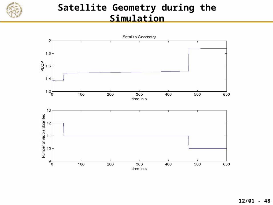
Satellite Geometry during the Simulation

12/01 - 49
Local Frame: x, y, z
Xecef
Yecef
Zecef
x
y
z
x=Zecef
y=-Yecef
z=Xecef-6378137m
Nominal Trajectory
)ft20000()m(6096h)s/ft200(
)s/m(61v
0
x

12/01 - 50
0 50 100 150 200 250 300 350 400-0.1
0
0.1
0.2
0.3Local Frame Velocity Errors
dvx
(m/s
)
0 50 100 150 200 250 300 350 400-0.2
-0.1
0
0.1
0.2
dvy
(m/s
)
gIgGwIgGwIwGgIwG
0 50 100 150 200 250 300 350 400-0.1
0
0.1
0.2
0.3
dvz
(m/s
)
time (s)0 400 (sec)
)s/m(dvx
)s/m(dvy
)s/m(dvz
Local Frame Velocity Errors: (true) – (estimated)
blue red (:) black (-.) green (--)INS good worse worse goodGPS good good worse worse
• GPS performance directly affects velocity errors


