Download - 3_Introduction to Nodal Analysis

7/28/2019 3_Introduction to Nodal Analysis
http://slidepdf.com/reader/full/3introduction-to-nodal-analysis 1/24

7/28/2019 3_Introduction to Nodal Analysis
http://slidepdf.com/reader/full/3introduction-to-nodal-analysis 2/24
= density,v = velocity,
d = pipe diameter, (ID),
g = acceleration due to gravity,
gc = garvity conversion factor,
f = fanning friction factor,
= pressure gradient,
m = mixture properties,
q = angle of inclination from horizontal
Multiphase Flow in Pipes
1. The pressure gradient equation for multi-phase flow can be written as:
dL g
dvv
d g 2
v f sin
g
g
dL
dp
c
mmm
c
2
mmm
c
q
Where:
dL
dp

7/28/2019 3_Introduction to Nodal Analysis
http://slidepdf.com/reader/full/3introduction-to-nodal-analysis 3/24
Multiphase Flow in Pipes

7/28/2019 3_Introduction to Nodal Analysis
http://slidepdf.com/reader/full/3introduction-to-nodal-analysis 4/24
Multiphase Flow in Pipes
7/28/2019 3_Introduction to Nodal Analysis
http://slidepdf.com/reader/full/3introduction-to-nodal-analysis 5/24
7/28/2019 3_Introduction to Nodal Analysis
http://slidepdf.com/reader/full/3introduction-to-nodal-analysis 6/24
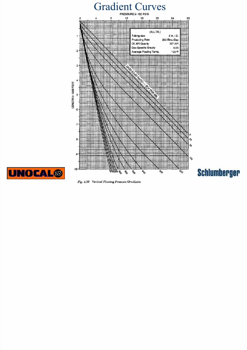
Gradient Curves

7/28/2019 3_Introduction to Nodal Analysis
http://slidepdf.com/reader/full/3introduction-to-nodal-analysis 7/24
Vertical Multiphase Flow: How to find the BHFP
7/28/2019 3_Introduction to Nodal Analysis
http://slidepdf.com/reader/full/3introduction-to-nodal-analysis 8/24
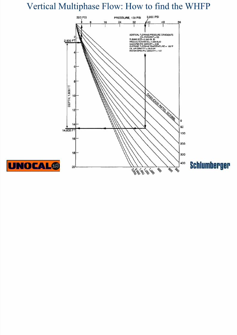
Vertical Multiphase Flow: How to find the WHFP
7/28/2019 3_Introduction to Nodal Analysis
http://slidepdf.com/reader/full/3introduction-to-nodal-analysis 9/24
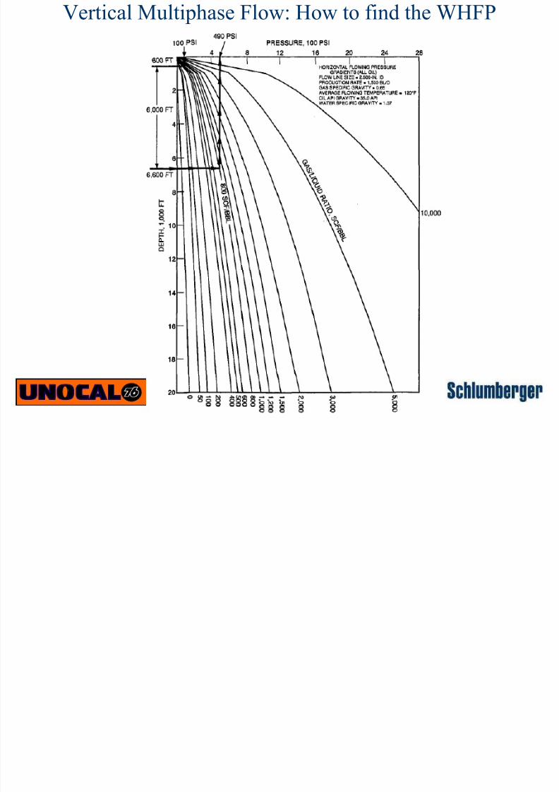
Vertical Multiphase Flow: How to find the WHFP
7/28/2019 3_Introduction to Nodal Analysis
http://slidepdf.com/reader/full/3introduction-to-nodal-analysis 10/24
Exercise:
Given:
Pwh=100 psig WH Temp.= 70o
FGLR = 400 scf/bbl BHST = 140o F
gg = 0.65 TD = 5,000 ft (mid – perf)
Tbg ID = 2.0 in API Gravity = 35o API
Calculate and plot the Tubing Intake Curve
Vertical Multiphase Flow: How to plot the
Tubing Intake Curve
7/28/2019 3_Introduction to Nodal Analysis
http://slidepdf.com/reader/full/3introduction-to-nodal-analysis 11/24
• Using Fig. 4.10, start at the top of the gradient curve at a pressure of
100 psig. Proceed vertically downward to a GLR of 400 scf/bbl.
Proceed horizontally and read an equivalent depth. Add the TVD to the
depth in question. Read a depth of 6,600 psig and proceed horizontally
to the 400 scf/bbl curve. From this point proceed vertically and read
the tbg intake pressure for 200 bpd of 720 psig.
• Repeat this procedure for flow rates of 400, 600, and 800 bpd using the
corresponding graphs.
• Plot the obtained values of Pwf to plot a Pwf vs q , the desired tubing
intake curve.
Vertical Multiphase Flow: How to plot the
Tubing Intake Curve

7/28/2019 3_Introduction to Nodal Analysis
http://slidepdf.com/reader/full/3introduction-to-nodal-analysis 12/24
Vertical Multiphase Flow: How to plot the
Tubing Intake Curve
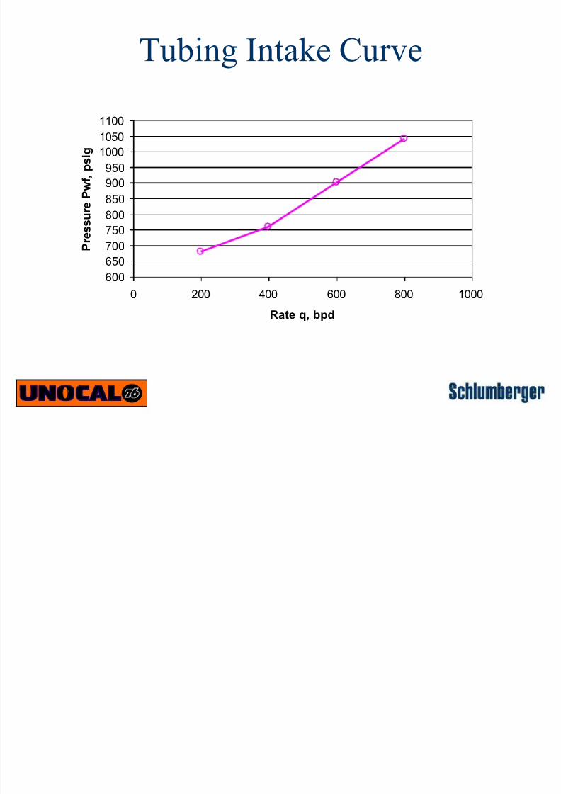
Assumed q, (bpd) Pwf , psig
200 720
400 730600 900
800 1000
7/28/2019 3_Introduction to Nodal Analysis
http://slidepdf.com/reader/full/3introduction-to-nodal-analysis 13/24
Tubing Intake Curve
600
650
700
750
800
850
900
950
1000
1050
1100
0 200 400 600 800 1000
Rate q, bpd
P r e s s u r e P
w f , p s i g

7/28/2019 3_Introduction to Nodal Analysis
http://slidepdf.com/reader/full/3introduction-to-nodal-analysis 14/24
Pressure Loss AcrossPerforations

7/28/2019 3_Introduction to Nodal Analysis
http://slidepdf.com/reader/full/3introduction-to-nodal-analysis 15/24
Pressure Loss in Perforations
• The effect of perforations on productivity can be
quite substantial.
• It is generally believed that if the reservoir
pressure is below the bubble point, causing 2 phase flow through the perforations, the pressure
loss may be an order of magnitude higher.
• 2 Methods for calculating presssure loss in
perforations, McLeod (1983) and Karakas
&Tariq (1988).
7/28/2019 3_Introduction to Nodal Analysis
http://slidepdf.com/reader/full/3introduction-to-nodal-analysis 16/24
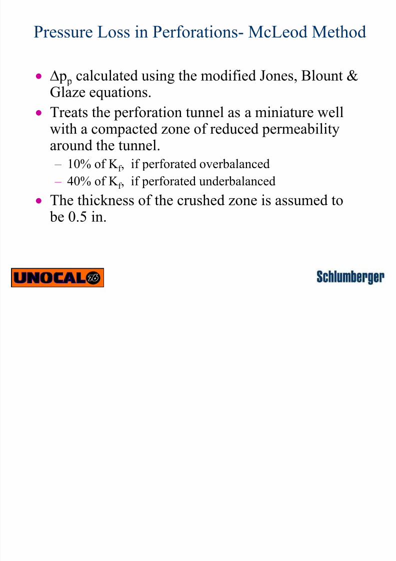
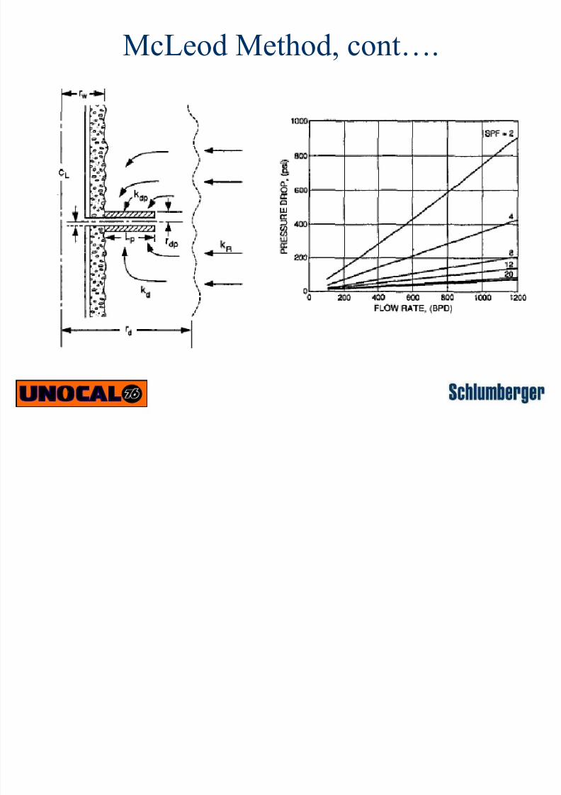
D p p calculated using the modified Jones, Blount &Glaze equations.
Treats the perforation tunnel as a miniature wellwith a compacted zone of reduced permeabilityaround the tunnel.
– 10% of K f , if perforated overbalanced
– 40% of K f , if perforated underbalanced
The thickness of the crushed zone is assumed to be 0.5 in.
Pressure Loss in Perforations- McLeod Method
7/28/2019 3_Introduction to Nodal Analysis
http://slidepdf.com/reader/full/3introduction-to-nodal-analysis 17/24
McLeod Method, cont….

7/28/2019 3_Introduction to Nodal Analysis
http://slidepdf.com/reader/full/3introduction-to-nodal-analysis 18/24
McLeod Method, cont….
• For an Oil well:
o
2
owf wfs bqaqPP
– where:
in5.0r r , k L10x08.7
r
r ln
b
k
10x2.33 ,
L
r
1
r
1
10x3.2a
pc
p p
3-
p
c
o
1.201
p
10
2
p
c p
2
o
14-
, q is flow rate through perforation

7/28/2019 3_Introduction to Nodal Analysis
http://slidepdf.com/reader/full/3introduction-to-nodal-analysis 19/24
McLeod Method, cont….
• For a gas well:
g
2
g
22 bqaqPPwf wfs
– where:
in5.0r r , k L
r
r lnTZ10x424.1
b
k
10x2.33 ,
L
r 1
r 1TZ10x16.3
a
pc
p p
p
c3
1.201
p
10
2
p
c p
g
12-
g
, qg is flow rate through perforation
7/28/2019 3_Introduction to Nodal Analysis
http://slidepdf.com/reader/full/3introduction-to-nodal-analysis 20/24
Karakas and Tariq Method, (1988)
• Semi-analytical solution to the problem of 3D
flow into a spiral system of perforations. Two
cases:
– 2D case, valid for small dimensionless perforationspacings (large perf penetration or high shot
density).
– 3D flow problem around the perf tunnel, valid inlow density perforations.
7/28/2019 3_Introduction to Nodal Analysis
http://slidepdf.com/reader/full/3introduction-to-nodal-analysis 21/24
Karakas and Tariq Method, cont…
t
w
e
wr
Sr
r ln
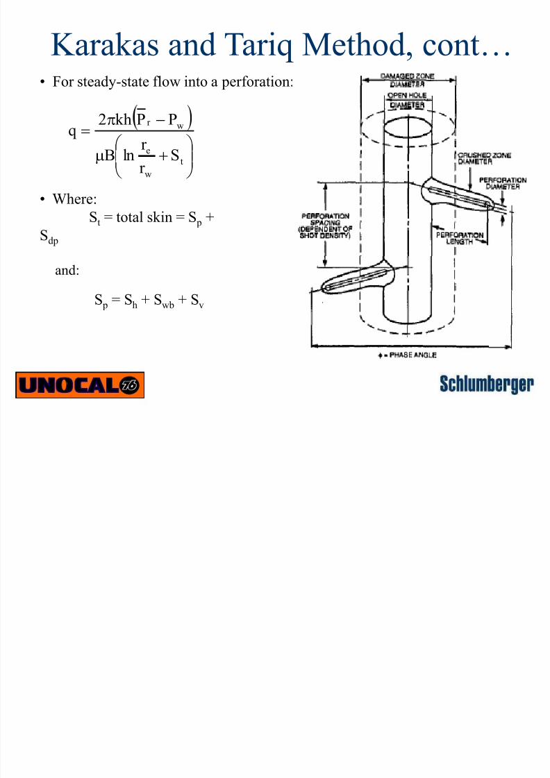
PPkh2q
• For steady-state flow into a perforation:
• Where:
St = total skin = S p +
Sdp
and:
S p = Sh + Swb + Sv

7/28/2019 3_Introduction to Nodal Analysis
http://slidepdf.com/reader/full/3introduction-to-nodal-analysis 22/24
S p = perforation skin factor Sdp= damage skin factor
Sh= pseudo skin due to phasing =
where: r we(q) is the effective wellbore radius as a function of the phasing angle (q)
and perf tunnel length. 0.25 l p , if q = 0o
rw(q) =
aq (r w + l p) , otherwise
Swb= pseudo skin due to wellbore effects (dominant in zero
degree phasing).
Sv= pseudo skin due to vertical converging flow (negligible in
the case of high shot density; 3D effect)
Karakas and Tariq Method, cont…
qwe
w
r
r ln

7/28/2019 3_Introduction to Nodal Analysis
http://slidepdf.com/reader/full/3introduction-to-nodal-analysis 23/24
Karakas and Tariq Method, cont…
Perforation
Phasingaq
(360o) 0o 0.250
180o
0.500120o 0.648
90o 0.726
60o 0.813
45
o
0.860
Dependance of aq on Phasing Swb(q) = C1(q) exp[C2(q)r wd]
Perforation
PhasingC1 C2
(360o) 0o 1.6E-1 2.675
180o
2.6E-2 4.532120o 6.6E-3 5.320
90o 1.9E-3 6.155
60o 3.0E-4 7.509
45
o
4.6E-5 8.791
7/28/2019 3_Introduction to Nodal Analysis
http://slidepdf.com/reader/full/3introduction-to-nodal-analysis 24/24
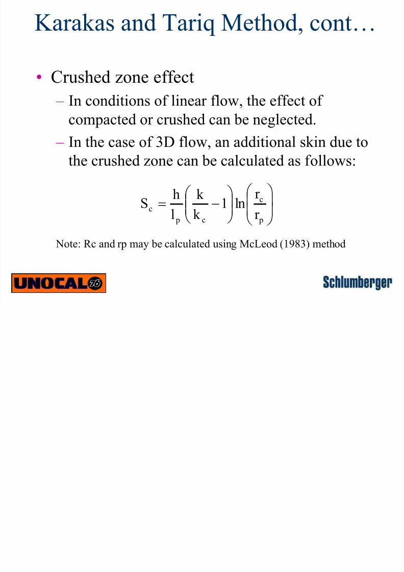
• Crushed zone effect
– In conditions of linear flow, the effect of
compacted or crushed can be neglected.
– In the case of 3D flow, an additional skin due tothe crushed zone can be calculated as follows:
Karakas and Tariq Method, cont…
p
c
c p
c
r
r ln1
k
k
l
hS
Note: Rc and rp may be calculated using McLeod (1983) method


