
1
Lecture 6: Simulation of Carrier and sampling frequency clock frequency error
March 28 – April 19 2008
Yuping Zhao (Doctor of Science in technology)
Professor, Peking UniversityBeijing, China
2
Carrier frequency error model
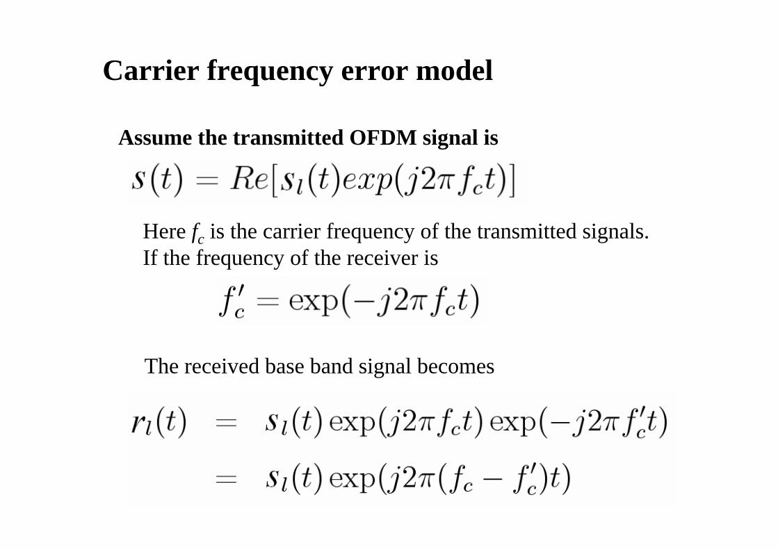
Assume the transmitted OFDM signal is
Here fc is the carrier frequency of the transmitted signals.If the frequency of the receiver is
The received base band signal becomes

3
The frequency difference is
If the sub-carrier separation is
The normalized frequency error is
4
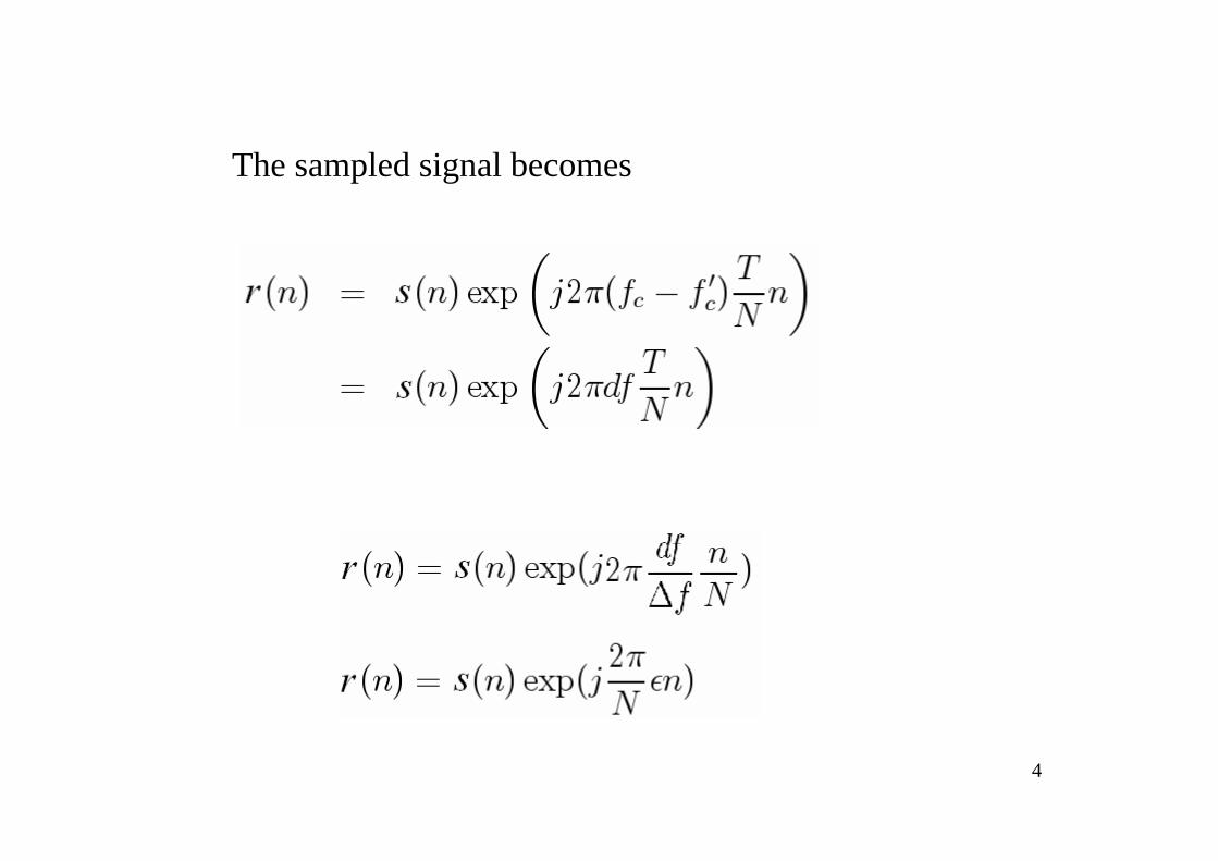
The sampled signal becomes

5
frequency error model of OFDM systems
X k s n r n Y k
π N εn
Frequencydomain
Frequencydomain
Timedomain
⎟⎠⎞
⎜⎝⎛−
Kn
Nj επ2exp
K is the up sample rate, ε is the normalized frequency error, here is 0.05

6
-3 -2 -1 0 1 2 30
0 .1
0 .2
0 .3
0 .4
0 .5
0 .6
0 .7
0 .8
0 .9
1
Amplitude Spectrum of OFDM

7
Influence of carrier frequency error to OFDM
• Assume the transmitted signal is:
Assume the carrier frequency error exist, then it can be expressed
is the AWGN samples
8
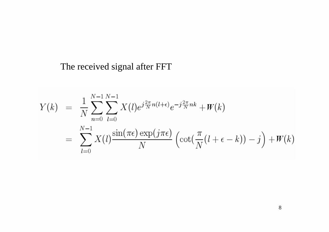
The received signal after FFT

9
The signal can be expressed as
Then

10
0 5 10-0.5
0
0.5
1
k
Re(
Y(k
))
The signal transmitted on sub-carrier 5 is 1+j

11
0 5 10-1
-0.5
0
0.5
1
1.5
k
Im(Y
(k))
The signal transmitted on subcarrier 5 is 1+j
12
0 5 100
0.5
1
1.5
k
ABS(
Y(k
))
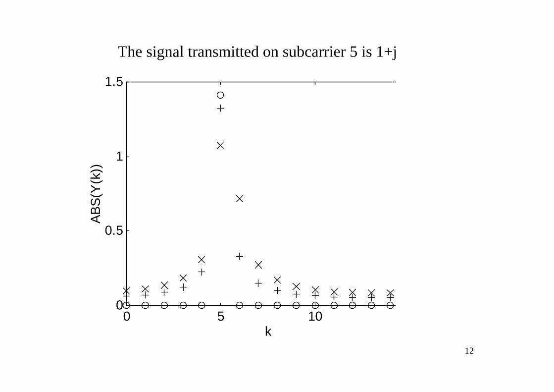
The signal transmitted on subcarrier 5 is 1+j

13
-5 0 5-5
-4
-3
-2
-1
0
1
2
3
4
5
Real
Imag
inar
y
ε = 5%
Figure.1

14
-6 -4 -2 0 2 4 6-6
-4
-2
0
2
4
6
Real
Imag
inar
y
ε = 25%
Figure.2

15
Frequency error correction method

16
Model of sampling clock frequency errors
t

17
0 2000 4000 6000 8000 10000 12000 14000-0.8
-0.6
-0.4
-0.2
0
0.2
0.4
0.6
0.8
Sampling timing error
Part 1 Part 2

18
Sampling timing error – part 1
300 400 500 600 700 800 900 1000 1100 1200
-0.6
-0.4
-0.2
0
0.2
0.4
0.6
Figure 3

19
1.18 1.19 1.2 1.21 1.22 1.23 1.24 1.25 1.26 1.27
x 104
-0.6
-0.4
-0.2
0
0.2
0.4
0.6
Sampling timing error – part 2
Figure 4

20
Clock frequency error problems
The correct sampling time
When the clock error exist, the received signal becomes
Here n’ is the practical sampling time

21
采样时钟偏差Constellation with Sampling frequency error
Figure.5
Error = 50ppm, r=0.5, delay=5
-4 -3 -2 -1 0 1 2 3 4-4
-3
-2
-1
0
1
2
3
4

22
采样时钟偏差Constellation with Sampling frequency error
Figure.6
-4 -3 -2 -1 0 1 2 3 4-4
-3
-2
-1
0
1
2
3
4
Error = 100ppm

23
Exercises 3-1: Clock and frequency errors simulations
Build a OFDM simulation system to show• Simulate the figure1-6 give in this ppt
Note: for the sampling clock error, you may use MATLAB function “resample”
----------------------------Example: 50ppm clock error:
P = 20000;Q = 19999; resampI = resample(filteredI,P,Q);resampQ = resample(filteredQ,P,Q);

24
Exercises 3-2: Fixed point simulations
Assume the synchronization of the received signal is perfect, the channel is AWGN. Convert the down sampled data into fixed value, examine how the system performance is affected by parameter A and K.
Case 1: K=5,8,13, the value A should not make truncation of the received signals
Case 2: K=10, the value A should chosen as 1) just suitable value; 2) with truncation; 3) too large compare with received signal value
------------------------------------------------For exercise 3-2, you may chose the parameters yourself

25
Instruction 3-1: carrier frequency error model
16QAM modulation
N-points IFFT
Guard insertion
Lowpass filtering
Binarydata
Lowpass filteringA/D converting
Guard deleting
N-points FFT
16QAM demodulation
Binarydata
X(k) x(n) x’(n) s(t)
y’(k) y(n) y’(n) r(t)
Up sampling
Down sampling
K is Up sampling rate, N is the FFT points,
show Signal constellation
⎟⎠⎞
⎜⎝⎛−
Kn
Nj επ2expX
is normalized frequency offset, its value is 5% and 25% in Figure 1 and Figure 2
⎟⎠⎞
⎜⎝⎛−
Kn
Nj επ2exp :

26
Instruction 3-2: clock frequency error model
16QAM modulation
N-points IFFT
Guard insertion
Lowpass filtering
Binarydata
Lowpass filteringA/D converting
Guard deleting
N-points FFT
16QAM demodulation
Binarydata
X(k) x(n) x’(n) s(t)
y’(k) y(n) y’(n)r(t)
Up sampling
Down sampling
show time domain Signal
resample
using MATLAB function “resample” to get the clock frequency error
(see next page)
r(n)
show Signal constellation

27
using MATLAB function “resample” to get the clock frequency error----------------------------Example: for 50ppm clock error:
P = 20000;Q = 19999;
real(y’) = resample(r_I,P,Q); % r_I is the real part of r(n) in the figureimag(y’) = resample(r_Q,P,Q); %r_Q is the imaginary part of r(n) in the figure
Note: The resample functionClock error = (P-Q)/P, however P and Q cannot be too big value, otherwise Matlabfunction cannot work
Instruction 3-2: clock frequency error model

28
Instruction 3-3: Fixed point simulation
16QAM modulation
N-points IFFT
Guard insertion
Lowpass filtering
Binarydata
Lowpass filteringA/D converting
Guard deleting
N-points FFT
16QAM demodulation
Binarydata
X(k) x(n) x’(n) s(t)
y’(k) y(n) y’(n)r(t)
Up sampling
Down sampling
show histogram
Fixed point model
Using fixed point function (see next page) for the fixed point simulation
r(n)
show signal constellation

29
Instruction 3-3: Fixed point simulation
Here is the fixed function (you also can make yourself)
----------------------------------------function Y = fixed(X,A,K)% X: input floating point data% A: The maximum value of the output, A>0% K: The number of bits for quantizationN = 2^(K-1) – 1;Y = round(min(A,max(X,-A))/A*N)/N*A-------------------------------------------------------For exercise 3-2, you may chose the parameters yourself. The following
figures are examples with different parameters.

30
-0.5 -0.4 -0.3 -0.2 -0.1 0 0.1 0.2 0.3 0.4 0.50
200
400
600
800
1000
1200Real part, floating point

31
-0.5 -0.4 -0.3 -0.2 -0.1 0 0.1 0.2 0.3 0.4 0.50
200
400
600
800
1000
1200Real part, fixed point, A = 0.4; K = 14

32
-4 -3 -2 -1 0 1 2 3 4-4
-3
-2
-1
0
1
2
3
4Real part, fixed point, A = 0.4; K = 14

33
-0.5 -0.4 -0.3 -0.2 -0.1 0 0.1 0.2 0.3 0.4 0.50
200
400
600
800
1000
1200Real part, fixed point, A = 0.25; K = 14

34
-4 -3 -2 -1 0 1 2 3 4-4
-3
-2
-1
0
1
2
3
4Real part, fixed point, A = 0.25; K = 14

35
-0.5 -0.4 -0.3 -0.2 -0.1 0 0.1 0.2 0.3 0.4 0.50
200
400
600
800
1000
1200Real part, fixed point, A = 0.2; K = 14

36
-4 -3 -2 -1 0 1 2 3 4-4
-3
-2
-1
0
1
2
3
4Real part, fixed point, A = 0.2; K = 14

37
-0.5 -0.4 -0.3 -0.2 -0.1 0 0.1 0.2 0.3 0.4 0.50
200
400
600
800
1000
1200Real part, fixed point, A = 0.4; K = 8

38
-4 -3 -2 -1 0 1 2 3 4-4
-3
-2
-1
0
1
2
3
4Real part, fixed point, A = 0.4; K = 8

39
-4 -3 -2 -1 0 1 2 3 4-4
-3
-2
-1
0
1
2
3
4Real part, fixed point, A = 0.4; K = 5

40


