Download - 72 BIWS O&G Valuation
7/31/2019 72 BIWS O&G Valuation
http://slidepdf.com/reader/full/72-biws-og-valuation 1/9
Oil & Gas Valuation – Quick Reference
http://breakingintowallstreet.co
Oil & Gas Valuation: Comparable Public Companies & Precedent Transactions
Picking a set of comparable companies or precedent transactions for an oil & gas company is very similar to
how you would pick them for any other company – here are the differences:
1. Rather than cutting the set by revenue or EBITDA, you would instead select the set based on Proved
Reserves or Daily Production (in addition to the normal geographic and industry criteria).
2. Instead of traditional metrics like revenue or EPS, you list the metrics and multiples that are relevant to
an energy company: EBITDAX, Proved Reserves, Daily Production, the Oil Mix %, and so on.
Please see the previous handout in this course on Oil & Gas Key Metrics to see the full list and to learn how to
calculate these metrics and multiples.
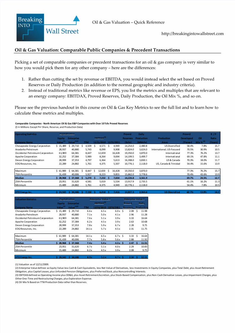
Comparable Companies ‐ North American Oil & Gas E&P Companies with Over 10 Tcfe Proved Reserves
($ in Millions Except Per Share, Reserve, and Production Data)
Operating Statistics Capitalization Proved Daily Proved R / P
Equity Enterprise EBITDAX(3)
Reserves Production Production Developed Oil Ratio
Company Name Value(1)
Value(1)(2)
TTM 12/31/2010 12/31/2011 (Bcfe) (MMcfe) Areas / Proved Mix %
(4)(Years)
Chesapeake Energy Corporation 15,489$ 29,710$ 4,509$ 4,571$ 4,949$ 14,254.0 2,480.8 US Diversified 58.4% 7.8% 15.7
Anadarko Petroleum 28,937 40,880 5,743 8,099 9,908 13,824.0 3,624.0 International; US‐Focused 70.5% 30.9% 10.5
Occidental Petroleum Corporation 61,989 64,381 8,447 12,659 16,428 19,350.0 3,870.0 Internati onal 77.3% 76.2% 13.7
Apache Corporation 32,252 37,384 5,989 8,264 9,694 14,199.5 3,499.7 Internati onal 69.1% 47.8% 11.1
Devon Energy Corporation 28,999 37,353 4,797 6,364 5,613 16,398.0 3,830.1 US & Canada 70.3% 18.0% 11.7
EOG Resources, Inc. 22,289 24,882 1,761 4,375 5,507 10,776.1 2,118.0 US, Canada & Trinidad 54.4% 15.6% 13.9
Maximum 61,989$ 64,381$ 8,447$ 12,659$ 16,428$ 19,350.0 3,870.0 77.3% 76.2% 15.7
75th
Percentile 31,439
40,006
5,927
8,223
9,855
15,862.0
3,778.6
70.4% 43.6% 13.9
Median 28,968$ 37,368$ 5,270$ 7,232$ 7,654$ 14,226.8 3,561.9 69.7% 24.5% 12.7
25th Percentile 23,951 31,620 4,581 5,019 5,534 13,917.9 2,735.5 61.1% 16.2% 11.3
Minimum 15,489 24,882 1,761 4,375 4,949 10,776.1 2,118.0 54.4% 7.8% 10.5
XTO Energy Inc. 24,542$ 34,686$ 7,150$ 6,818$ 7,416$ 14,827.3 2,863.6 US Diversified 60.7% 13.9% 14.2
Valuation Statistics Capitalization Enterprise Value / Enterprise Value /
Equity Enterprise EBITDAX(3)
Prove d Dail y
Company Name Value(1)
Value(1)(2)
TTM 12/31/2010 12/31/2011 Reserves Production
Chesapeake Energy Corporation 15,489$ 29,710$ 6.6 x 6.5 x 6.0 x 2.08$ 11.98$
Anadarko Petroleum 28,937 40,880 7.1 x 5.0 x 4.1 x 2.96 11.28
Occidental Petroleum Corporation 61,989 64,381 7.6 x 5.1 x 3.9 x 3.33 16.64
Apache Corporation 32,252 37,384 6.2 x 4.5 x 3.9 x 2.63 10.68
Devon Energy Corporation 28,999 37,353 7.8 x 5.9 x 6.7 x 2.28 9.75
EOG Resources, Inc. 22,289 24,882 14.1 x 5.7 x 4.5 x 2.31 11.75
Maximum 61,989$ 64,381$ 14.1 x 6.5 x 6.7 x 3.33$ 16.64$
75th Percentile 31,439 40,006 7.7 x 5.8 x 5.6 x 2.88 11.92
Median 28,968$ 37,368$ 7.4 x 5.4 x 4.3 x 2.47$ 11.51$
25th Percentile 23,951 31,620 6.7 x 5.1 x 4.0 x 2.29 10.83
Minimum 15,489 24,882 6.2 x 4.5 x 3.9 x 2.08 9.75
XTO Energy Inc. 24,542$ 34,686$ 4.9 x 5.1 x 4.7 x 2.34$ 12.11$
(1) Valuation as of 12/11/2009.
(2) Enterprise Value defined as Equity Value less Cash & Cash Equivalents, less Net Value of Derivatives, less Investments in Equity Companies, plus Total Debt, plus Asset Retirement
Obligation, plus Capital Leases, plus Unfunded Pension Obligations, plus Preferred Stock, plus Noncontrolling Interests.
(3) EBITDAX defined as Operating Income plus DD&A, plus Asset Retirement Accretion, plus Stock‐Based Compensation, plus Non‐Cash Derivative Losses, plus Impairment Charges, plus
Other One‐Time and Restructuring Charges, plus Exploration Expense.
(4) Oil Mix % Based on TTM Production Data rather than Reserves.

7/31/2019 72 BIWS O&G Valuation
http://slidepdf.com/reader/full/72-biws-og-valuation 2/9
Oil & Gas Valuation – Quick Reference
http://breakingintowallstreet.co
Precedent Transactions are similar as well – use geography, industry, transaction size, and possibly reserves /
daily production to select the deals and then use the oil & gas‐specific metrics and multiples.
Common Add‐Backs and Non‐Recurring Charges
When calculating EBITDA or EBITDAX, there are a couple items specific to oil & gas to watch out for:
Asset Retirement Accretion (a form of amortization)
Non‐Cash or Unrealized Derivative (Gains) / Losses (appears on the cash flow statement)
Impairment Charges and PP&E Write‐Downs (more common with full cost companies)
(Gain) / Loss on Sale of Assets (appears on the cash flow statement)
Environmental Remediation
You need to read the footnotes carefully because sometimes these charges are already included in DD&A or
are capitalized and don’t hit the income statement at all.
Here’s an example of charges we would add back for Chesapeake Energy, one of XTO’s comps:
But there may be additional charges hidden in the cash flow statement and in the footnotes so we need look
there as well:

7/31/2019 72 BIWS O&G Valuation
http://slidepdf.com/reader/full/72-biws-og-valuation 3/9
Oil & Gas Valuation – Quick Reference
http://breakingintowallstreet.co
We’re not adding the other charges on the cash flow statement either 1) because they’re already included in
the income statement add‐ backs (e.g. the loss on the sale of PP&E), or 2) because they do not hit the operating
income (e.g. loss from equity investments) – read the footnotes carefully.
Discounted Cash Flow Analysis
You can still build a DCF model for oil & gas companies and it’s almost
the same as what you see for normal companies:
You start with Revenue and move down to EBIT, subtract taxes,
and then add back non‐cash charges.
At the end you still subtract the increase or add the decrease in
Working Capital and subtract CapEx to get to Unlevered FCF.
You still discount the cash flows in the same way, applying a mid‐
year discount if you want.
You still calculate the Terminal Value using multiples or long‐term growth rates.
You still
calculate
WACC
just
like
you
would
for
a normal
company.
The key differences with an oil & gas DCF:
You will have additional non‐cash expenses in addition to the standard ones like DD&A and Stock‐
Based Compensation.
You would use Daily Production, EBITDA, or EBITDAX for the terminal exit multiples rather than a
Free Cash Flow‐ based multiple.

7/31/2019 72 BIWS O&G Valuation
http://slidepdf.com/reader/full/72-biws-og-valuation 4/9
Oil & Gas Valuation – Quick Reference
http://breakingintowallstreet.co
For the Gordon Growth method usually you assume 0% long‐term growth because oil & gas assets get
depleted over time and there’s only a finite amount in the ground.
You could use the oil & gas industry standard 10% discount rate rather than calculating WACC. For the sensitivity tables you would look at commodity prices as one of the variables rather than
revenue growth or EBITDA margins; other variables might be the discount rate and terminal growth
rates or terminal multiples.
DCFs generally do not work well for oil & gas companies because:
They have a high CapEx requirement, which reduces Free Cash Flow and may create declining or
negative Free Cash Flow.
As a result, they are even more dependent on the Terminal Value than normal companies – so the
analysis doesn’t
tell
you
much.
An alternative is the Net Asset Value (NAV) model , which streamlines the traditional DCF and makes it more
applicable to oil & gas companies.
Net Asset Value (NAV) Models
A NAV model is an alternative to a DCF that gives more accurate
results for oil & gas companies, especially for companies with an
upstream or exploration & production focus (i.e. they focus on
finding and
producing
energy
rather
than
on
refining
energy
or
marketing it).
The major differences compared to a traditional DCF:
1. A NAV model assumes that the company never increases
its existing reserves, so there is no additional CapEx in
future years beyond what is required to develop existing
reserves.
2. A DCF model is done at the corporate level, but you run a NAV model at the asset level. You value a
company’s
assets
separately
and
then
add
everything
together
at
the
end
–
whereas
with
a
DCF
you
arevaluing the entire company from the start.
With a DCF you’re saying, “This company operates and keeps earning profit indefinitely into the future – how
much is it worth right now?” but with a NAV you’re saying, “This company stops operating once its reserves
are depleted – how much profit can it generate between now and then, assuming no future re‐investment to
find or acquire new reserves?”
Here’s how to create a Net Asset Value model:

7/31/2019 72 BIWS O&G Valuation
http://slidepdf.com/reader/full/72-biws-og-valuation 5/9
Oil & Gas Valuation – Quick Reference
http://breakingintowallstreet.co
Resource Prices for NAV: Gas Oil / NGL Hedged
$ per Mcf $ per Bbl Price %
7.00$ 75.00$ 110.0%
Price Cased Used in NAV: NAV
Step 1: Make Assumptions for Reserves, Production, Commodity Prices, Future Costs, and Discount Rates
Most of these will flow in from other parts of your model or from the company’s annual filing. In the example model here, we have projections for the first 5 years and then have to extrapolate beyond that in the NAV.
Proved Reserves as of 12/31/2009: Long‐Term Production Decline:
Natural Gas (Bcf): 12,502 Natural Gas: (5.0%)
Natural Gas Liquids (MBbls): 93 Natural Gas Liquids: (5.0%)
Oil (MBbls): 294 Oil: (5.0%)
Natural Gas Equivalents (Bcfe): 14,827
Future Estimated Development Costs: 8,484$ Discount Rate: 10.0%
Development Years 5
The Proved Reserves numbers come directly from the filing. Future estimated development costs come from
the PV‐10 section of the company’s filing, and we estimate that it will take 5 years to fully develop all their
existing Proved Reserves:
The discount rate of 10% is the standard used in the oil & gas industry and what you always see in companies’
filings.
We have the production numbers for the next 5 years, but past that we need to make our own assumptions as
the reserves get depleted – so we are making a simple estimate here and assuming a 5% decline each year for
natural gas,
NGLs,
and
oil.
For commodity prices, you assume the same numbers
for oil and NGLs and different numbers for natural gas
and the hedging percentage; these numbers should
flow through the rest of your model from the NAV and
will give you averaged realized prices for the first 5 years.

7/31/2019 72 BIWS O&G Valuation
http://slidepdf.com/reader/full/72-biws-og-valuation 6/9
Oil & Gas Valuation – Quick Reference
http://breakingintowallstreet.co
Revenue ($ in Millions)
Natural Total
Gas Oil & NGL Revenue
6,438$ 2,390$ 8,828$
7,081 2,629 9,711
7,811 2,844 10,655
8,374 3,049 11,422
9,002 3,277 12,279
8,552 3,113 11,665
8,124 2,958 11,082
7,718 2,810 10,528
7,332 2,669 10,001
6,965 776 7,742
6,617 ‐ 6,617
1,558 ‐ 1,558
‐ ‐ ‐
Natural Gas
Beginning Annual Avg.
Reserves Production Price
Year # (Bcf) (Bcf) $ / Mcf
2010 1 12,502 941 6.84$
2011 2 11,561 1,035 6.84
2012 3 10,527 1,141 6.84
2013 4 9,385 1,223 6.84
2014 5 8,162 1,315 6.84
Step 2: Project Production and Realized Prices for Commodities
For this one, let’s take natural gas as an example and look at the first 5 years here:
The annual production is pulled directly from our production
model, and we are assuming roughly a 10% production increase
in the first 3 years followed by a 7‐8% increase in years 4 and 5.
The realized prices are also coming from our existing
assumptions, flowed
all
the
way
through
the
model.
The beginning Proved Reserves balance declines by the annual
production each year.
We are adding in a MIN formula to make sure that the annual production never drops below 0.
In the years beyond this initial 5‐year period, you:
Continue to decrease the reserves balance by
the annual production.
Straight‐line the average realized sale prices, i.e.
assume a constant $6.84 for all future years here
based on our price assumptions above.
For the annual production, you take the MIN of
the beginning reserves balance and the previous
year’s production multiplied by (1 + Long‐Term
Production Decline Rate) – that ensures that production declines over time but never drops below the
reserves from the beginning of the year.
You carry those formulas through the next 20 or 30 years (determine the period
based on the Reserve Life Ratio).
Then you multiply the average realized price each year by the annual production
each year for each commodity and sum up everything to get annual revenue.

7/31/2019 72 BIWS O&G Valuation
http://slidepdf.com/reader/full/72-biws-og-valuation 7/9
Oil & Gas Valuation – Quick Reference
http://breakingintowallstreet.co
Step 3: Make Expense and Tax Assumptions and Calculate After‐Tax Cash Flows
Since the Net Asset Value model is done at an asset level , you do not include corporate overhead expenses such as G&A. For oil & gas you usually just include production and development expenses, and assume a tax
rate based on the historical numbers:
Production & Development Expenses: Cash Flows ($ in Millions)
Total Total
Annual Production Production Development Pre‐Tax Cash After‐Tax
Bcfe Per Mcf e Expe ns es Expe nse s Cash Flows Tax Rate Cash Flows
1,150 0.95$ 1,092$ 1,697$ 6,039$ 11.8% 5,327$
1,265 0.95 1,201 1,697 6,812 11.8% 6,009
1,391 1.00 1,391 1,697 7,567 11.8% 6,675
1,491 1.00 1,491 1,697 8,235 11.8% 7,264
1,603
1.00
1,603
1,697
8,980
11.8% 7,921
1,522 1.00 1,522 ‐ 10,143 11. 8% 8,947
1,446 1.00 1,446 ‐ 9,636 11. 8% 8,499
1,374 1.00 1,374 ‐ 9,154 11. 8% 8,075
1,305 1.00 1,305 ‐ 8,696 11. 8% 7,671
1,086 1.00 1,086 ‐ 6,655 11. 8% 5,871
967 1.00 967 ‐ 5,650 11. 8% 4,984
228 1.00 228 ‐ 1,331 11. 8% 1,174
‐ 1.00 ‐ ‐ ‐ 11.8% ‐
The first 5 years of production expenses and tax rates flow in directly from our operating model; after that we
assume constant expenses per Mcfe and a constant tax rate. For the annual development expenses, we take the
total from
the
assumptions
at
the
top
and
divide
by
the
assumed
development
period,
5 years
in
this
case.
At the end, we take revenue and subtract production, development, and taxes to calculate the after‐tax cash
flows.
Step 4: Take the Net Present Value of the After‐Tax Cash Flows
This is just a simple NPV formula in Excel – apply it to the range that the After‐Tax Cash Flows column covers
You should use the standard 10% oil & gas discount for the NAV_Discount_Rate variable here.
Step 5: Value the Other Assets
So far, we have included only the after‐tax cash flows from oil & gas exploration and production activities.
But natural resource companies frequently have other business segments: midstream (transporting the energy)
refining & marketing (turning it into usable gas / oil and selling it to customers), and chemicals.

7/31/2019 72 BIWS O&G Valuation
http://slidepdf.com/reader/full/72-biws-og-valuation 8/9
Oil & Gas Valuation – Quick Reference
http://breakingintowallstreet.co
Enterprise Value: 48,444$
Balance Sheet Adjustments: (10,144)
Implied Equity
Value: 38,300$
Diluted Shares Outstanding: 598.6
Implied Share Price: 63.99$
Exercise
Type: Number: Price: Dilution:
Options 18.366 38.39$ 7.347
RSU 5.493 5.493
Performance Shares A 0.390 50.00 0.390
Performance Shares B 0.228 55.00 0.228
Performance Shares C 0.245 77.00 ‐
Performance Shares D 0.245 85.00 ‐
Warrants 2.600 20.78 1.756
Undeveloped Acres (Property Values in $ Millions USD):
Region: Acres: $ / Acre: Value:
US ‐ Texas: 281,000 1,500$ 422$
US ‐ Oklahoma: 176,000 500 88
US ‐ New Mexico: 21,000 300 6
US ‐ Arkansas: 216,000 700 151
US ‐ Montana: 92,000 500 46
US ‐ Utah: 84,000 400 34
US ‐ Louisiana: 39,000 700 27
US ‐ North Dakota: 191,000 500 96
US ‐ Kansas: ‐ 500 ‐
US ‐ West Virginia: 58,000 600 35
US ‐ Pennsylvania: 119,000 1,200 143
US ‐ Wyoming: 13,000 400 5
US ‐ Colorado: 2,000 500 1
US ‐ Other: 76,000 300 23
US ‐ Offshore: 45,000 400 18
North Sea ‐ Offshore: 133,000 600 80
Total: 1,546,000 759$ 1,174$
They also have undeveloped land that has value even if it
doesn’t count as Proved Reserves or if nothing has been
produced yet.
First, estimate the value for the undeveloped land (see Excel
paste‐in on the right).
You can get estimates for $ / Acre or total undeveloped land
value from equity research or from industry sources like the
Herold Database.
If XTO actually had other business segments, here’s how we
might estimate
the
value
of
each
one:
Other Business Segments:
Chemicals Midstream Downstream
12/31/2009 EBITDA: 200$ 12/31/2009 EBITDA: 100$ 12/31/2009 EBITDA: 150$
EV/EBITDA Multiple: 5.0 x EV/EBITDA Multiple: 3.0 x EV/EBITDA Multiple: 3.0 x
Estimated EV: 1,000$ Estimated EV: 300$ Estimated EV: 450$
To do this more rigorously, you would select public comps for each segment and base the EBITDA multiple on
those.
Once you have the value of the undeveloped land and the other business segments, you add up all of those
and the Present Value of After‐Tax Cash Flows from Proved Reserves to get the Enterprise Value:
Step 6: Make Balance Sheet Adjustments and Calculate the Implied Per Share Price
Once you have the Enterprise Value, you work
backwards (i.e.
add
cash,
subtract
debt,
and
so
on)
to
get
to Equity Value and calculate the implied per share
price – just like you would for a normal company.
When you’re finished and you have the per share price,
you can then create sensitivity tables based on
commodity prices and the other assumptions at the top
of the model.

7/31/2019 72 BIWS O&G Valuation
http://slidepdf.com/reader/full/72-biws-og-valuation 9/9
Oil & Gas Valuation – Quick Reference
http://breakingintowallstreet.co
You would not use metrics like revenue growth or EBITDA margins because once again, they are not
applicable to oil & gas companies.
Mining, Footnotes, and More
You can also create NAV models for mining and other natural resource
companies.
They’re very similar – the main difference is that you make additional
assumptions on the revenue side (e.g. you might assume that only a certain
percentage of the tons mined have the metal you’re looking for, or that a
certain percentage are “wasted” in the mining process).
You don’t have to create a NAV model exactly like the example we went through above – here are some
variations you will see:
We used Proved Reserves (1P) here but you can also use Proved + Probable Reserves (2P) or Proved +
Probable + Possible Reserves (3P). You will see references to 1P NAV, 2P NAV, 3P NAV, and so on in
equity research.
You will see many variations on the expense and tax assumptions because they are company‐
dependent. The safest bet is to follow what they do in the PV‐10 calculation in their filings.
You could value the other business segments by using a segment‐level DCF or other methods rather
than just
assuming
a simple
EBITDA
multiple
as
we
did
here.
Finally, note that NAV models are most applicable to exploration & production‐focused natural resource
companies.
If a company is more focused on transporting energy or refining and selling it, they are not as dependent on
assets as an E&P company so you would stick to the standard public comps, precedent transactions, and DCF
there.


