
1
A bit from the Physics and mesoscale side
Content
• Model cycles in 2008
• Clouds: verification and future
• Convective gusts
• A bit about recent tropical cyclones
• Mesoscale convective systems
• Present and future of middle atmosphere

2
21212121°CCCC
Today 12 UTC
3
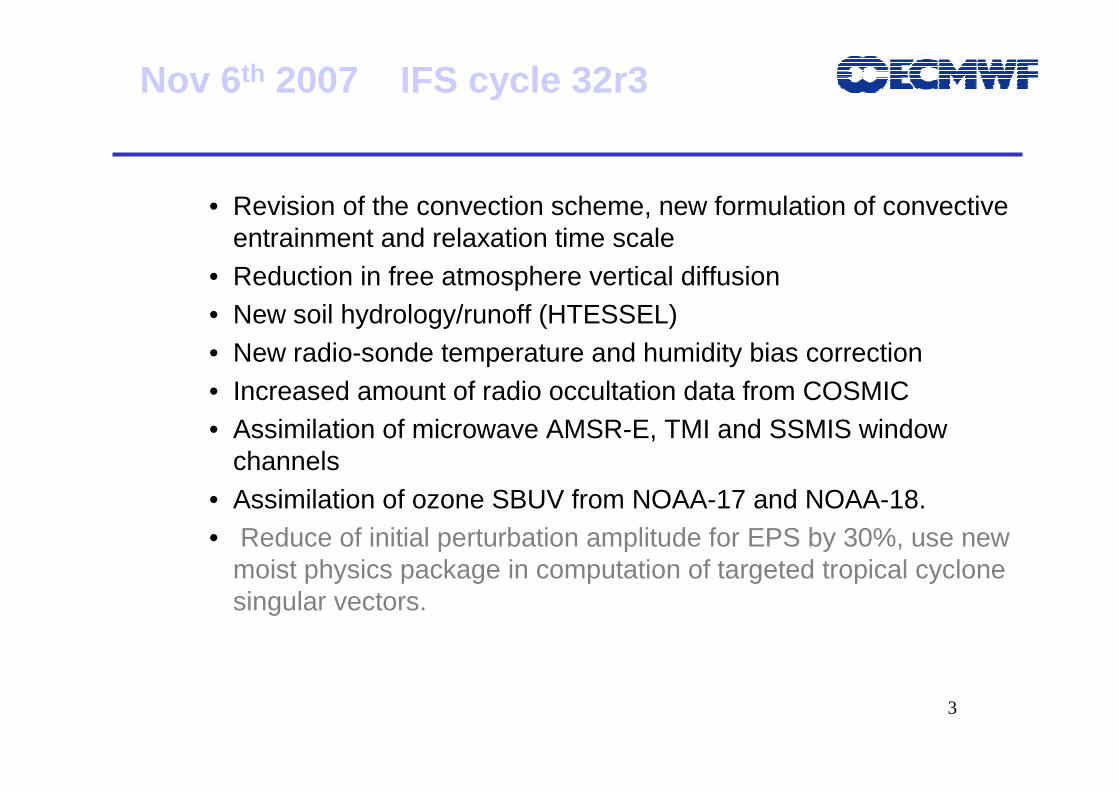
Nov 6th 2007 IFS cycle 32r3
• Revision of the convection scheme, new formulation of convectiveentrainment and relaxation time scale
• Reduction in free atmosphere vertical diffusion• New soil hydrology/runoff (HTESSEL)• New radio-sonde temperature and humidity bias correction• Increased amount of radio occultation data from COSMIC• Assimilation of microwave AMSR-E, TMI and SSMIS window
channels• Assimilation of ozone SBUV from NOAA-17 and NOAA-18.• Reduce of initial perturbation amplitude for EPS by 30%, use new
moist physics package in computation of targeted tropical cyclone singular vectors.

4
Feb 3rd 2008 IFS cycle 33r1
• Improved moist physics in tangent linear/adjoint of 4D-Var.• Physics: Retuned entrainment in convection scheme. Bugfix to
scaling of freezing term in convection scheme. Additional shear term in diffusion coefficient of vertical diffusion. Increased turbulent orographic form drag. Fix for soil temperature analysis in areas with 100% snow cover. Change in surface roughness for momentum.
• Modified post-processing of 2m T and q. • Active assimilation of AMSR-E and TMI rainy radiances.• Use of 4 wind solutions for QuikSCAT. • Extended coverage and increased resolution of limited area wave
model.• Improved shallow water physics and modified advection for ocean
wave model.

5
Sept 30th 2008 IFS cycle 35r1
– OSTIA sea surface temperature and sea ice analysis – Conserving interpolation scheme for trajectory – New VARBC bias predictors to allow the correction of IR shortwave
channels affected by solar effects – Cleaner cold start of AMSUA channel 14 – New physics for melting of falling snow – Increased albedo of permanent snow cover – Cool skin/warm layer SST parametrization– Revised linear physics – Add convective contribution to wind gusts in post-processing – Monitoring of MERIS data

6
Equitable threat score for European precipitation against SYNOP data
Curves show 12 month running mean of seasonal values
Calendar Years
1 day per 7 years

7
Winter Cloud Cover : 36h forecast versus SYNOP observation (for high pressure days over central Europe (last four winters))
DJF
2004/558 cases
DJF
2005/660 cases
DJF
2007/869 cases
DJF
2006/752 cases
EDMF PBL
M-O diffusion

8
Cloud Overlap
• Cloud overlap assumption for cloud diagnostics made consistent with radiation scheme. (“exponential maximum-random” overlap).
• Identified differences and impacts between old and new cloud overlap assumptions.
• Fixed long-term bug in medium and low level cloud diagnostics (MCC, LCC)

9
Cloud VerificationObs-to-Model: Ice water content
Model ice water content (excluding precipitating
snow).
Ice water content derived from a 1DVAR retrieval of CloudSat/
CALIPSO/Aqua
log10
kg m-3
R. Forbes + M. Ahlgrimm
Eq EqEq GreenlandAntarctica
26/02/2007 15Z

10
Cloud VerificationModel-to-Obs: Radar reflectivity
Simulated radar reflectivity from the
model.(ice only)
Observed radar reflectivity from
CloudSat(ice + rain)
Tropics 82°N82°S
0°C
0°C
26/02/2007 15Z
R. Forbes + M. Ahlgrimm

11
Cloud VerificationTropical Cloud Height and Depth
1 year CloudSat data 20°S-20°N
Snapshot of ECMWF model 06 Aug 2008 (20°S-20°N)
R. Forbes + M. Ahlgrimm

12
New 5-prognostic cloud microphysicsFalling snow and orographic forcing
Wind
Surface Precipitation(36 hour acc.) Orography
“Prognostic snow scheme”minus “Diagnostic snow scheme”
(36 hour acc) (1 year average)
“Prognostic snow scheme”minus “Diagnostic snow scheme”

13
Proposition: Use low-level wind shear multiplied by mixing parameter α<1 when deep convection is active
Other formulations trying to simulate cold pool gust fronts using downdraught W or evaporation have been unsuccessful (too large perturbations over Oceans and in Tropics)
Convective Gusts
Motivation: report about gust front by DWD22 February 2008
10 850 950max(0, )gustconvU U Uα= −

14
Wind gustscase 22 February 2008 continued
Obs
Oper Conv

15
Wind gustssummertime example 25 June 2008
Obs
Oper Conv

16
Wind 10m + gusts verif over SeaBuoy verification

H
HH
L
L
L
L
L
1010
1010
1010
1020
1020
15°N
20°N
25°N
30°N
35°N
95°W
95°W 90°W
90°W 85°W
85°W 80°W
80°W 75°W
75°W 70°W
70°W 65°W
65°W 60°W
60°W 55°W
55°W 50°W
50°W 45°W
45°W 40°W
40°W 35°W
35°W
W ednesday 27 August 2008 00UTC ECMWF Forecast t+132 VT: Monday 1 September 2008 12UTC Surface: Mean sea level pressure
FC 27th Aug 0Z t+132 VT: 1st Sept
ANALYSIS VT: 1st Sept H
H
H
H
H
H
H
L
L
L
L
L
1010
1010
1010
1010
1020
1020
15°N
20°N
25°N
30°N
35°N
95°W
95°W 90°W
90°W 85°W
85°W 80°W
80°W 75°W
75°W 70°W
70°W 65°W
65°W 60°W
60°W 55°W
55°W 50°W
50°W 45°W
45°W 40°W
40°W 35°W
35°W
ECMWF Analysis VT:Monday 1 September 2008 12UTC Surface: Mean sea level pressure
IKE
GustavGustavGustavGustav
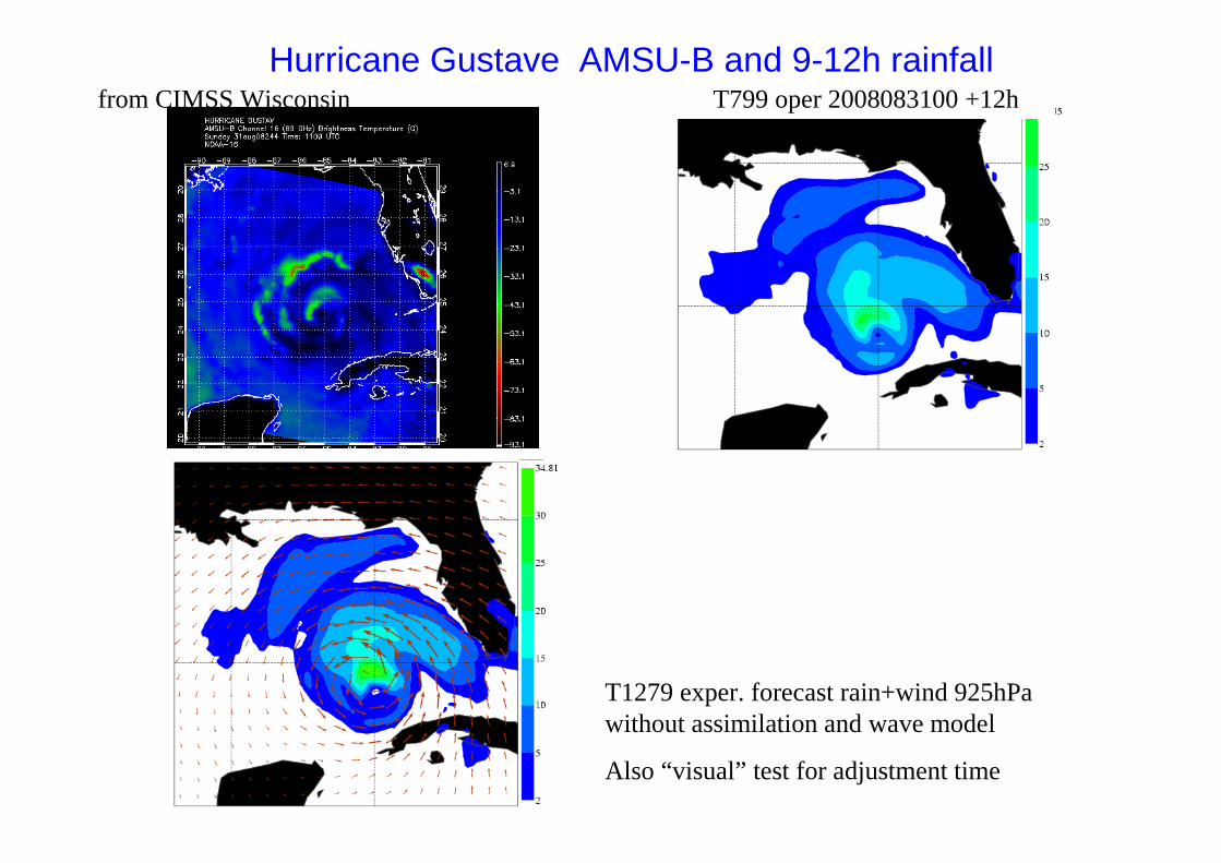
Hurricane Gustave AMSU-B and 9-12h rainfallfrom CIMSS Wisconsin
T1279 exper. forecast rain+wind 925hPa without assimilation and wave model
Also “visual” test for adjustment time
T799 oper 2008083100 +12h
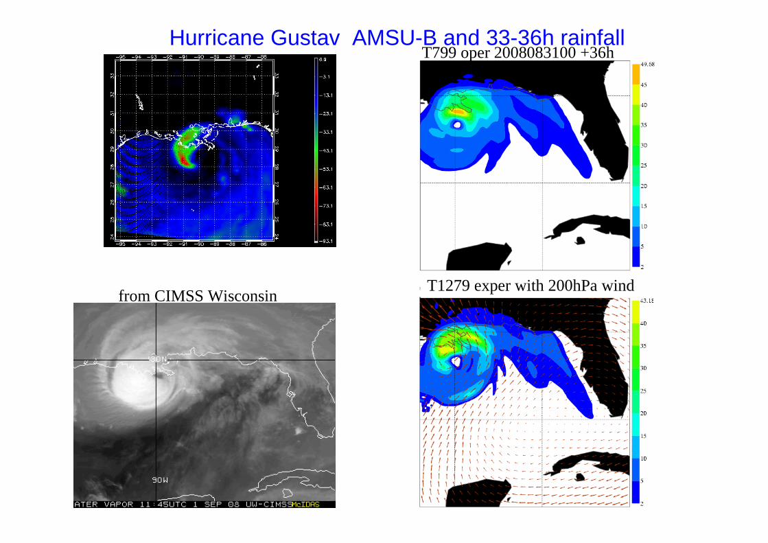
Hurricane Gustav AMSU-B and 33-36h rainfall
from CIMSS Wisconsin
T799 oper 2008083100 +36h
T1279 exper with 200hPa wind
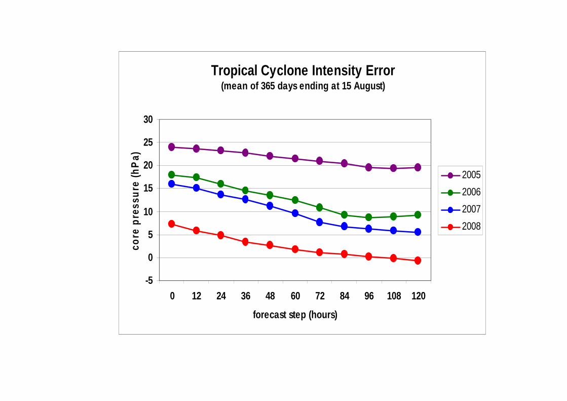
Tropical Cyclone Intensity Error(mean of 365 days ending at 15 August)
-5
0
5
10
15
20
25
30
0 12 24 36 48 60 72 84 96 108 120
forecast step (hours)
core
pre
ssu
re (
hP
a)
2005
2006
2007
2008

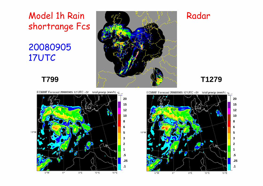
Model 1h Rain Radarshortrange Fcs
2008090515UTC
20
15
12
10
8
6
5
3
2
1
.5
.25
.1
20
15
12
10
8
6
5
3
2
1
.5
.25
.1
T799 T1279

Model 1h Rain Radarshortrange Fcs
2008090516UTC
20
15
12
10
8
6
5
3
2
1
.5
.25
.1
20
15
12
10
8
6
5
3
2
1
.5
.25
.1
T799 T1279
Model 1h Rain Radarshortrange Fcs
2008090517UTC
20
15
12
10
8
6
5
3
2
1
.5
.25
.1
20
15
12
10
8
6
5
3
2
1
.5
.25
.1
T799 T1279

Model 1h Rain Radarshortrange Fcs
2008090518UTC
20
15
12
10
8
6
5
3
2
1
.5
.25
.1
20
15
12
10
8
6
5
3
2
1
.5
.25
.1
T799 T1279
25
Conclusion rainfall Maps
• T1279 looks subjectively ok and even more realistic, results (rainrates) are quasi resolution independent
• First assimilation tests of Radar rainrates (NEXRAD, planned is to use European archive) have been carried out by Philippe Lopez
• We know that we probably overestimate very small rainrates

Research project
Run a Cloud Resolving Model initialised with IFS Analysisover large domains and study:
• Interaction of convection and dynamics through “diabatic heating”(including cold pools), and the propagation and upscale evolution of mesoscale convective systems.
• Diurnal cycle
• momentum flux in squall lines (line-normal one is upgradient)
• Identify and possible resolve deficiencies in IFS related to these issues.
Realisation:
• Use the Meso-nh model in collaboration with J.P Chaboureau
• Focus on large mesoscale systems during AMMA using AMMA (Anna) reanalyses
• currently CRM resolution is set to 5 km, IFS is run at T511 (40 km) like Reanalysis, and first T1279 (15 km) forecasts are under way

27
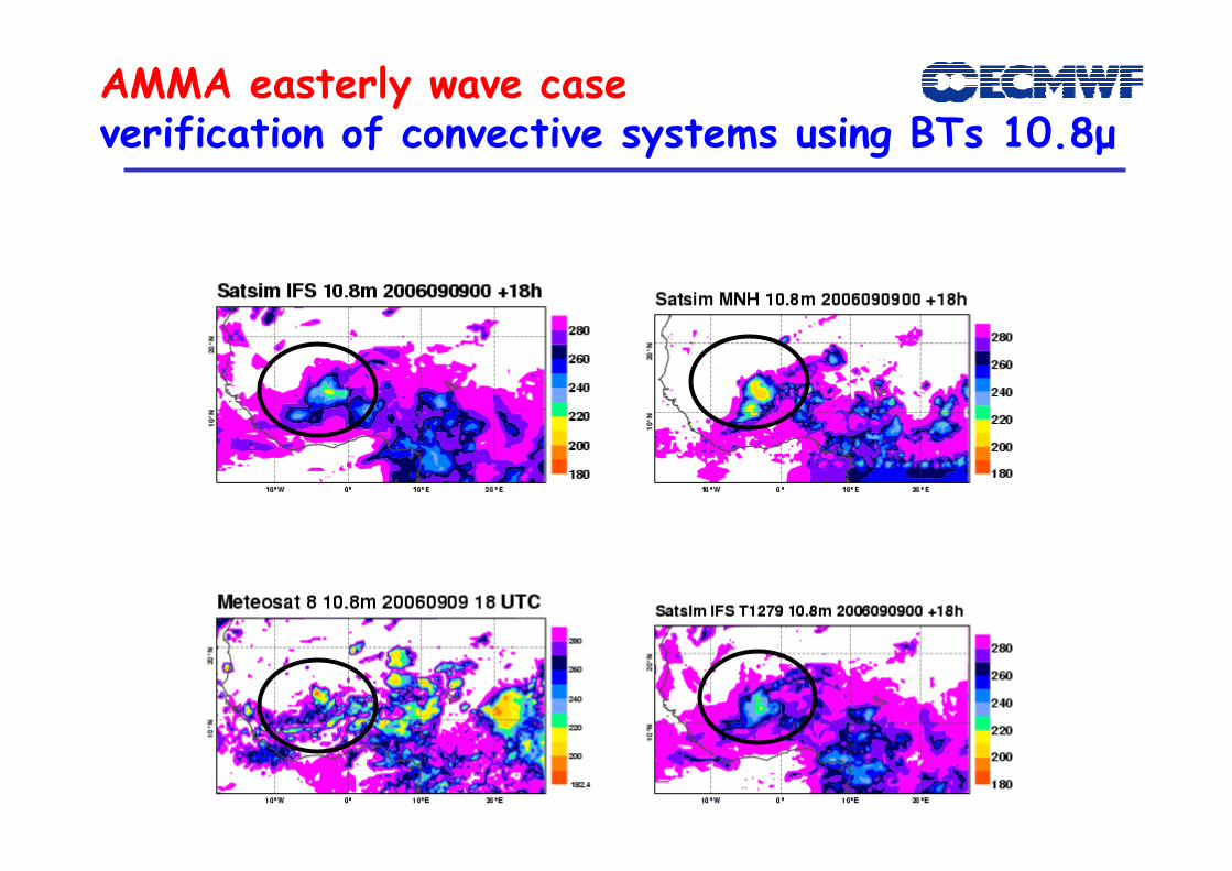
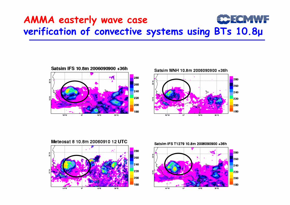
Ex of AMMA easterly wave case 36hverification of convective systems using BTs 10.8µ
All images interpolated to T511 grid

28
AMMA easterly wave caseverification of convective systems using BTs 10.8µ
29
AMMA easterly wave caseverification of convective systems using BTs 10.8µ

30
AMMA easterly wave caseverification of convective systems using BTs 10.8µ

31
AMMA easterly wave caseverification of convective systems using BTs 10.8µ
32
AMMA easterly wave caseverification of convective systems using BTs 10.8µ

33
AMMA easterly wave caseverification of convective systems using BTs 10.8µ
Both models produce low-level cold and warm inflow for mesoscalesystem

34
AMMA easterly wave caseverification of 925 T
Reasonable in both models, a bit more mesoscale system dynamics in Meso-nh

35
AMMA easterly wave caseverification of 200hPa U
Probably too strong system and upper level divergence (outflow in Meso-nh)

Preliminar statements
• 4 periods of 48h have bun run including easterly and non-easterly wave cases, and a case with convection penetrating into the stratosphere
• the IFS at 40 km and 15 km and the Meso-nh explicit at 5 km produce similar results in terms of success in producing and propagating mesoscale systems; the biases with respect to Reanalysis are also similar. Meso-nh produces some more systems but the onset of convection tends to be sometimes delayed by a few hours compared to observations, and upper-level outflow overestimated.
• cases with strong forcing (easterly waves) better represented
• need to do more data analysis
• Heating profiles still have to be produced for Meso-nh and analysed using e.g. EOFs

37
The ECMWF middle atmosphere climate and the parameterization of non-orographic gravity wavesby A. Orr +A. Untch +N.Wedi

50 OS 0O 50 ON1000600400
200
1006040
20
1064
2
10.60.4
0.2
0.10.060.04
0.02
200
220
220
220
240
240
240
260
260
260
Jan 32R3 T (K)
50 OS 0O 50 ON1000600400
200
1006040
20
1064
2
10.60.4
0.2
0.10.060.04
0.02
200
220
220
220
240
240
240
260
260
260
Jan 33R1 T (K)
50 OS 0O 50 ON1000600400
200
1006040
20
1064
2
10.60.4
0.2
0.10.060.04
0.02
200
200
220
220
220
240
240
240
260
260
260
Jan 33R1+CLIM_GHG T (K)
50 OS 0O 50 ON1000600400
200
1006040
20
1064
2
10.60.4
0.2
0.10.060.04
0.02
200
200
220
220
220
240
240
240
260
260
260
Jul 32R3 T (K)
50 OS 0O 50 ON1000600400
200
1006040
20
1064
2
10.60.4
0.2
0.10.060.04
0.02
200
200
220
220
220
240
240
240
260
260
260
Jul 33R1 T (K)
50 OS 0O 50 ON1000600400
200
1006040
20
1064
2
10.60.4
0.2
0.10.060.04
0.02200
220
220
220
240
240
240
260
260
Jul 33R1+CLIM_GHG T (K)
50OS 0O 50ON1000
600400
200
1006040
20
1064
2
10.60.4
0.2
0.10.060.04
0.02
200
220
220
220
240
240
240
260
260
Jan OBS T (K)
50OS 0O 50ON1000
600400
200
1006040
20
1064
2
10.60.4
0.2
0.10.060.04
0.02
220
220
240
240
240
260
260
Jul OBS T (K)
50 OS 0O 50 ON1000600400
200
1006040
20
1064
2
10.60.4
0.2
0.10.060.04
0.02
-30 -10
-1 0
0
20
Jan 32R3 U (m/s)
50 OS 0O 50 ON1000600400
200
1006040
20
1064
2
10.60.4
0.2
0.10.060.04
0.02
-30 -10
- 10
0
20
Jan 33R1 U (m/s)
50 OS 0O 50 ON1000600400
200
1006040
20
1064
2
10.60.4
0.2
0.10.060.04
0.02
-30 -10
-10
0
20
Jan 33R1+CLIM_GHG U (m/s)
50 OS 0O 50 ON1000600400
200
1006040
20
1064
2
10.60.4
0.2
0.10.060.04
0.02
-30
-10
-10
0
20
20
40 6080
80
100
Jul 32R3 U (m/s)
50 OS 0O 50 ON1000600400
200
1006040
20
1064
2
10.60.4
0.2
0.10.060.04
0.02
-30
-10
-10
0
20
20
40 6080
80
Jul 33R1 U (m/s)
50 OS 0O 50 ON1000600400
200
1006040
20
1064
2
10.60.4
0.2
0.10.060.04
0.02
-30
-10
-10
0
0
20
20
40
40
6080
80
Jul 33R1+CLIM_GHG U (m/s)
50OS 0O 50ON1000
600400
200
1006040
20
1064
2
10.60.4
0.2
0.10.060.04
0.02
-50-30
-100
20
Jan OBS U (m/s)
50OS 0O 50ON1000
600400
200
1006040
20
1064
2
10.60.4
0.2
0.10.060.04
0.02
-30
-10
0
20
40
40
60
80
Jul OBS U (m/s)
Mean January and July zonal-mean temperature and zonal wind for observations (top), 32R3 (second top), 33R1 (third top), and 33R1 + CLIM_GHG (lower). Simulations are 8-year (1994-2001) averages.
SPARC observed climatology
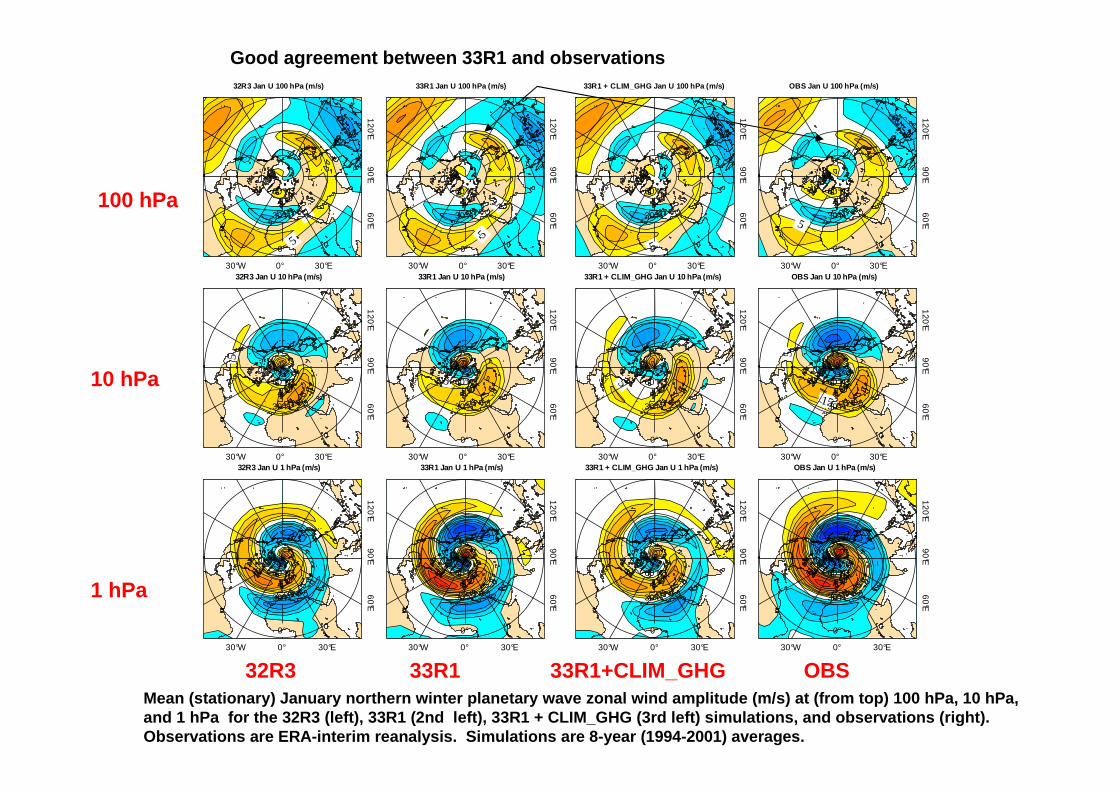
32R3NH planetary wave activity over-estimated (Bechtold et al. 2008)
33R1NH planetary wave activity better, but still biases
33R1 + improved GHG (O3,CO2,CH4, N2O, CFC11, CFC12, CFC22, CC14) climatology (D. Cariolle, JJ Morcrette, A Untch)Towards realistic temperature and circulation.
Jan July Jan July
0°
30°N
60°N
180°150°W
30°W 0° 30°E
60°E90
°E120
°E
150°E32R3 Jan U 1 hPa (m/s)
5
0°
30°N
60°N
180°150°W
30°W 0° 30°E
60°E90°E
120°E
150°E32R3 Jan U 10 hPa (m/s)
5
50°
30°N
60°N
180°150°W
30°W 0° 30°E
60°E90°E
120°E
150°E32R3 Jan U 100 hPa (m/s)
0°
30°N
60°N
180°150°W
30°W 0° 30°E
60°E90
°E120
°E
150°E33R1 Jan U 1 hPa (m/s)
5
0°
30°N
60°N
180°150°W
30°W 0° 30°E
60°E90°E
120°E
150°E33R1 Jan U 10 hPa (m/s)
55
0°
30°N
60°N
180°150°W
30°W 0° 30°E
60°E90°E
120°E
150°E33R1 Jan U 100 hPa (m/s)
0°
30°N
60°N
180°150°W
30°W 0° 30°E
60°E90
°E120
°E
150°E33R1 + CLIM_GHG Jan U 1 hPa (m/s)
5
0°
30°N
60°N
180°150°W
30°W 0° 30°E
60°E90°E
120°E
150°E33R1 + CLIM_GHG Jan U 10 hPa (m/s)
50°
30°N
60°N
180°150°W
30°W 0° 30°E
60°E90°E
120°E
150°E33R1 + CLIM_GHG Jan U 100 hPa (m/s)
0°
30°N
60°N
180°150°W
30°W 0° 30°E
60°E90
°E120
°E
150°EOBS Jan U 1 hPa (m/s)
5
15
0°
30°N
60°N
180°150°W
30°W 0° 30°E
60°E90°E
120°E
150°EOBS Jan U 10 hPa (m/s)
5
0°
30°N
60°N
180°150°W
30°W 0° 30°E
60°E90°E
120°E
150°EOBS Jan U 100 hPa (m/s)
Mean (stationary) January northern winter planetary wave zonal wind amplitude (m/s) at (from top) 100 hPa, 10 hPa, and 1 hPa for the 32R3 (left), 33R1 (2nd left), 33R1 + CLIM_GHG (3rd left) simulations, and observations (right). Observations are ERA-interim reanalysis. Simulations are 8-year (1994-2001) averages.
Good agreement between 33R1 and observations
100 hPa
10 hPa
1 hPa
32R3 33R1 33R1+CLIM_GHG OBS
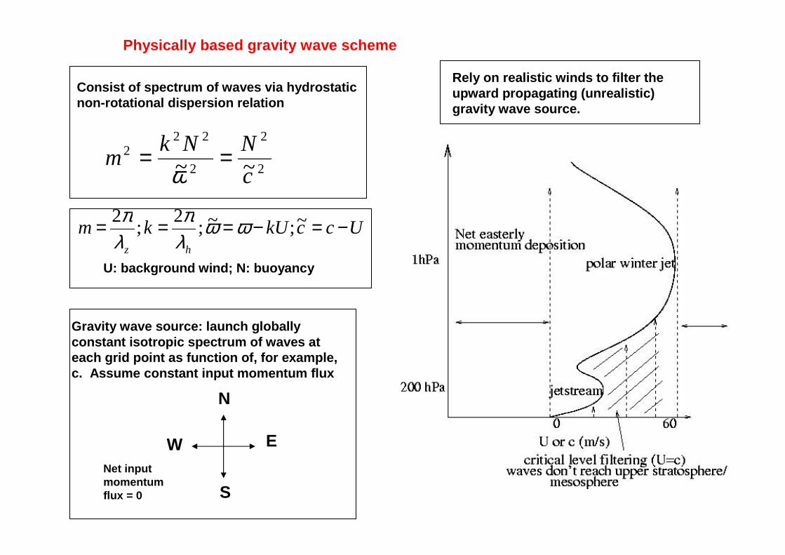
Gravity wave source: launch globally constant isotropic spectrum of waves at each grid point as function of, for example, c. Assume constant input momentum flux
Consist of spectrum of waves via hydrostatic non-rotational dispersion relation
2
2
2
222
~~ c
NNkm ==
ω
UcckUkmhz
−=−=== ~;~;2
;2 ωω
λπ
λπ
U: background wind; N: buoyancy
N
EW
S
Net input momentum flux = 0
Rely on realistic winds to filter the upward propagating (unrealistic) gravity wave source.
Physically based gravity wave scheme

50OS 0O 50ON1000
600400
200
1006040
20
1064
2
10.60.4
0.2
0.10.060.04
0.02
200
200
220
220
220
240
240
240
260
260
(a) Jul RF T (K)
50 O S 0O 50 ON1000600400
200
1006040
20
1064
2
10.60.4
0.2
0.10.060.04
0.02
200
220
220
220
240
240
240
260
260
(c) Jul WMS T (K)
50 O S 0O 50 ON1000600400
200
1006040
20
1064
2
10.60.4
0.2
0.10.060.04
0.02
220
220
240
240
240
260
260
(e) Jul OBS SPARC T (K)
50 O S 0O 50 ON1000600400
200
1006040
20
1064
2
10.60.4
0.2
0.10.060.04
0.02
200
220
220240
240
240
260
260
(g) Jul OBS ERAI T (K)
50OS 0O 50ON1000600400
200
1006040
20
1064
2
10.60.4
0.2
0.10.060.04
0.02
-30
-10
-10
0
0
20
20
40
40
6080
80
(b) Jul RF U (m/s)
50 OS 0O 50 ON1000
600400
200
1006040
20
1064
2
10.60.4
0.2
0.10.060.04
0.02
-30 -1
0
0
0
20
20
4060 8 0
(d) Jul WMS U (m/s)
50 OS 0O 50 ON1000
600400
200
1006040
20
1064
2
10.60.4
0.2
0.10.060.04
0.02
-30
-10
0
20
40
40
60
80
(f) Jul OBS SPARC U (m/s)
50 OS 0O 50 ON1000
600400
200
1006040
20
1064
2
10.60.4
0.2
0.10.060.04
0.02
-30
-10
20
20
4060
80
(h) Jul OBS ERAI U (m/s)
50OS 0O 50ON1000
600400
200
1006040
20
1064
2
10.60.4
0.2
0.10.060.04
0.02
200
200
220
220
220
240
240
240
260
260
260
(a) Jan RF T (K)
50 O S 0O 50 ON1000600400
200
1006040
20
1064
2
10.60.4
0.2
0.10.060.04
0.02
200
220
220
220
240
240
240
260
260
260
(c) Jan WMS T (K)
50 O S 0O 50 ON1000600400
200
1006040
20
1064
2
10.60.4
0.2
0.10.060.04
0.02
200
220
220
220
240
240
240
260
260
(e) Jan OBS SPARC T (K)
50 O S 0O 50 ON1000600400
200
1006040
20
1064
2
10.60.4
0.2
0.10.060.04
0.02
200
220
220
240
240
240
260
260
(g) Jan OBS ERAI T (K)
50OS 0O 50ON1000600400
200
1006040
20
1064
2
10.60.4
0.2
0.10.060.04
0.02
-30 -10
- 10
0
20
(b) Jan RF U (m/s)
50 OS 0O 50 ON1000
600400
200
1006040
20
1064
2
10.60.4
0.2
0.10.060.04
0.02
-50-30-10
-10
0
20 40
(d) Jan WMS U (m/s)
50 OS 0O 50 ON1000
600400
200
1006040
20
1064
2
10.60.4
0.2
0.10.060.04
0.02
-50-30
-100
20
(f) Jan OBS SPARC U (m/s)
50 OS 0O 50 ON1000
600400
200
1006040
20
1064
2
10.60.4
0.2
0.10.060.04
0.02
-30
-10
20
(h) Jan OBS ERAI U (m/s)
Mean January and July zonal-mean temperature and zonal wind for Rayleigh friction (RF) and W and McIntyre (1996), Scinoccia (2003) scheme and observations. Simulations are 33R1 + CLIM_GHG 8-year (1994-2001) averages.
RF
WMS
OBSSPARC
OBSERAI

-40
-40
-40
-30
-30
-30-30
-30
-30
-30
-30-30
-30
-30
-30
-30-30
-30
-20
-20
-20
-20
- 20
-20 -20-20 -20
-20
-20
-20-20
-20
-20
-20
-20-20
-20 -20
-10
-10
-10
-10
-10
-10
-10
-10
-10
-10
-10-10
-10-10
5 5
5
5
0.01
0.02
0.05
0.1
0.2
0.5
1
2
5
10
20
406080100
200
4006008001000
RF U (m/s>
-60-55-55-50-50-45-45-40-40-35-35-30-30-25-25-20-20-15-15-10-10-55101015152020252530303535404045455050555560
-30
-20
-20
-20
-20
-20
-20
-20
-20
-20
-20
-20
-20
-10
-10
-10
-10
-10
-10
-10
-10-10
-10
-10
-10 -10
-10
-10
-1 0
-10
-10
-10 -10 -10
-10
-10
-10
-10
5
55
0.01
0.02
0.05
0.1
0.2
0.5
1
2
5
10
20
406080100
200
4006008001000
1994 1995 1996 1997 1998 1999 2000 2001
WMS U (m/s)
-60-55-55-50-50-45-45-40-40-35-35-30-30-25-25-20-20-15-15-10-10-55101015152020252530303535404045455050555560
-40
-40
-30
-30
-30
-30
-30-30
- 20
-20
-20
-20
-20
-20
-20-20
-20
-20-20
-20-20
-20-10
-10
-10
-10
-10
-1 0 -10
-10-10
-10
-10
-10
-10
5
5
5 5
5
5
5
5 5 51
2
5
10
20
40
6080
100
200
400
600800
1000
1994 1995 1996 1997 1998 1999 2000 2001
OBS U (m/s)
-60-55-55-50-50-45-45-40-40-35-35-30-30-25-25-20-20-15-15-10-10-55101015152020252530303535404045455050555560
Monthly mean zonally averaged zonal wind over the equator for the RF (upper) and WMS (middle) simulations, and observations (lower). Observations are ERAI reanalysis up to 1 hPa for the 1994-2001 period. The winds have been meridionally averaged between 10oS and 10oN.
RF has easterly bias due to use of Rayleigh friction which damps U to zero
Westerly shear zone not captured?
Semi-annual oscillation (period~6 months)Quasi-biennial oscillation (period ~ 27 months)

43
Realistic QBO in tropics?
DSP produces waves carrying the necessary westerly momentum flux
Monthly mean zonally averaged zonal wind over the equator for the RF (top) and DSP (middle) simulations, and observations (lower). The observations consist of ERAI reanalysis for the 1994 to 2001 period. The simulation results are for the same period. The winds have been meridionally averaged between 10S and 10N. The contour interval is 5 m/s.
-30
-30
-20 -20
-20
-20
-20-20
-10
-10-10
-10
-10
-10
55 5
0.01
0.02
0.05
0.1
0.2
0.5
1
2
5
10
20
50
100
200
500
1000
1994 1995 1996 1997 1998 1999 2000 2001
RF U (m/s>
-60-55-55-50-50-45-45-40-40-35-35-30-30-25-25-20-20-15-15-10-10-55101015152020252530303535404045455050555560
-30 -30
-30
-30-30 -20
-20-20
-20
-20
-10
-10
-10
-10
-10
-10
-10 -10
5
5
5
5
5
5
15 15
0.01
0.02
0.05
0.1
0.2
0.5
1
2
5
10
20
50
100
200
500
1000
1994 1995 1996 1997 1998 1999 2000 2001
DSP U (m/s)
-60-55-55-50-50-45-45-40-40-35-35-30-30-25-25-20-20-15-15-10-10-55101015152020252530303535404045455050555560
-30
-30
-30
-20
-20
-20
-20
-10
-10
-10
-10
-10
5
55
1
2
5
10
20
50
100
200
500
1000
1995 1996 1997 1998 1999 2000 2001
OBS U (m/s)
-60-55-55-50-50-45-45-40-40-35-35-30-30-25-25-20-20-15-15-10-10-55101015152020252530303535404045455050555560

44
Hope to get this implemented within one year, together with new GHG climatology (monthly values instead annual average, and covering period 18xx to 2100) … need to maintain probably a bit Raileighfriction at model top


