
A Local Adaptive Approach for Dense Stereo Matching in Architectural Scene
Reconstruction
C. Stentoumis1, L. Grammatikopoulos2, I. Kalisperakis2, E. Petsa2, G. Karras1
1. Laboratory of Photogrammetry, Department of Surveying,
National Technical University of Athens, GR-15780 Athens, Greece
2. Laboratory of Photogrammetry, Department of Surveying,
Technological Educational Institute of Athens, GR-12210 Athens, Greece
5th International Workshop on 3D Virtual Reconstruction and Visualization of Complex Architectures (3D-ARCH '2013), 25-26 February 2013
1

Outline
• Introduction
• Related Work
• Proposed Algorithm
• Experimental Results
• Conclusion
2

Introduction
3

Objective
• Present a method
• Combines pre-existing algorithms and novel considerations
• With good sub-pixel accuracy
4

Related work
5

Related Work
6
Stereo Matching :
14
5
Range: 0 - 16
(X,Y) (X-d,Y)
Related Work
7
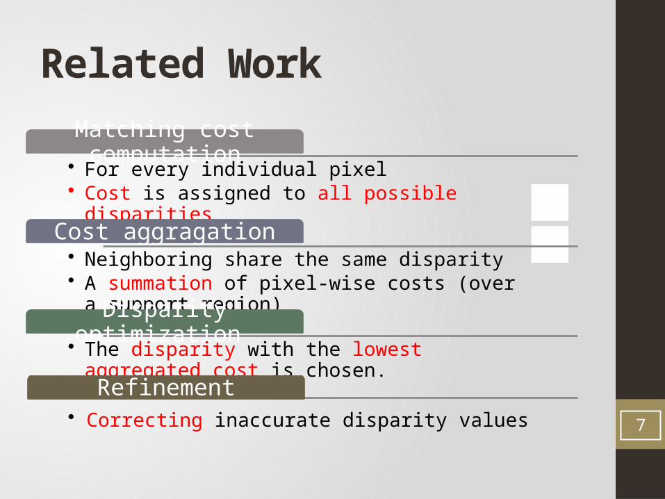
Matching cost computation• For every individual pixel• Cost is assigned to all possible disparities
Cost aggragation• Neighboring share the same disparity• A summation of pixel-wise costs (over a support region)
Disparity optimization • The disparity with the lowest aggregated cost is chosen.
Refinement• Correcting inaccurate disparity values

ProposedAlgorithm
8

Census on intensity principal derivatives
• Census transformation based on gradients:• Less sensitive to radiometric differences and repetitive
patterns
9
Intensity
Gradient

Census on Gradients
10
1 1 0 0 0
1 1 0 0 0
1 1 X 0 0
0 0 0 1 1
1 1 1 1 1
0.7 0.8 0.3 0.2 0.3
0.6 0.6 0.4 0.3 0.2
0.6 0.7 0.5 0.4 0.1
0.4 0.4 0.3 0.6 0.6
0.6 0.7 0.6 0.7 0.7
1 1 0 0 0 1 1 0 0 0 1 1 0 0 0 0 0 1 1 1 1 1 1 1
Census transform window :

Hamming Distance
11
• Left image
• Right image
Hamming Distance = 3
1 1 0 0 0 1 1 0 0 0 1 1 0 0 0 0 0 1 1 1 1 1 1 1
1 1 1 0 0 1 1 0 0 1 0 1 0 0 0 0 0 1 1 1 1 1 1 1
XOR
0 0 1 0 0 0 0 0 0 1 1 0 0 0 0 0 0 0 0 0 0 0 0 0

Comparison
• After aggregation step:
Default census Census on gradients
2.5% less erroneous pixels
12

Comparison
• After aggregation step[13]:
13
[13]Mei X., Sun X., Zhou M., Jiao S., Wang H., Zhang X., 2011. On building an accurate stereo matching system on graphics hardware. ICCV Workshop on GPU in Computer Vision Applications.

Absolute Difference on Image Color and Gradients
•
•
14
AD ( color ) :
AD ( Gradient ) :

Total Matching Cost
•
• normalized by λ
15
AD (color)Census (gradient) AD (gradient)
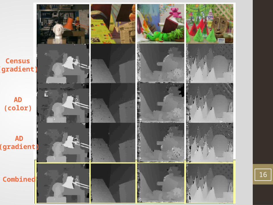
16
Census(gradient)
AD(color)
AD(gradient)
Combined

Support Region
17
• Cross-based support region[25]:
• Threshold of cross-skeleton expansion:
[25]Zhang K., Lu J., Lafruit G., 2009. Cross-based local stereo matching using orthogonal integral images. IEEE Transactions on Circuits & Systems for Video Technology.
Support Region
18
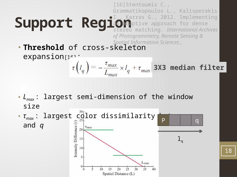
• Threshold of cross-skeleton expansion[16]:
• Lmax : largest semi-dimension of the window size
• τmax : largest color dissimilarity between p and q
3X3 median filter
[16]Stentoumis C., Grammatikopoulos L., Kalisperakis I., Karras G., 2012. Implementing an adaptive approach for dense stereo matching. International Archives of Photogrammetry, Remote Sensing & Spatial Information Sciences,
P q
lq

Support Region
19
Aggregation Step
20
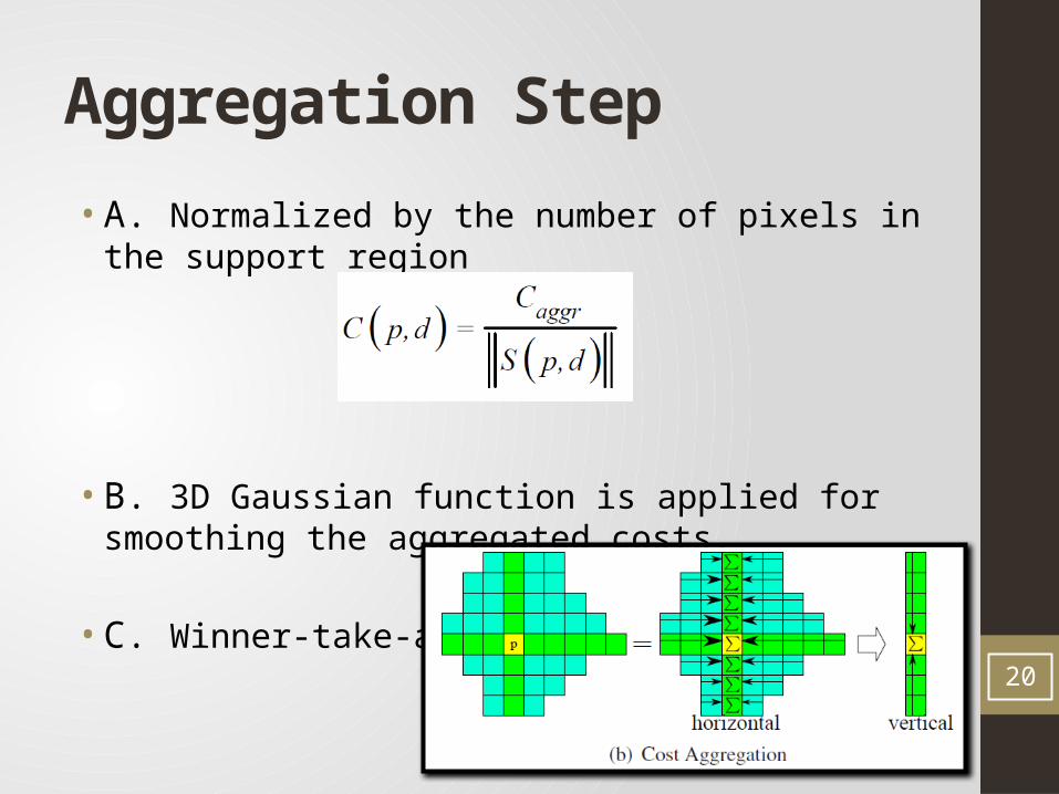
• A. Normalized by the number of pixels in the support region
• B. 3D Gaussian function is applied for smoothing the aggregated costs.
• C. Winner-take-all

Comparison
• After aggregation step[13]:
21Run this step for 4 iterations to get stable cost values. For iteration 1 and 3, aggregated horizontally and then vertically. For iteration 2 and 4, aggregated vertically and then horizontally.

•
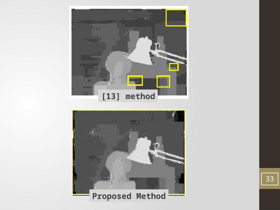
22
[13] method
Proposed Method
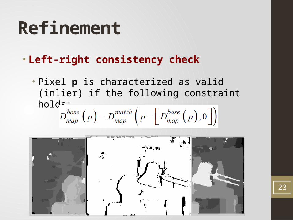
Refinement
23
• Left-right consistency check
• Pixel p is characterized as valid (inlier) if the following constraint holds:

Refinement
24
• Outlier cross-based filtering
• The cross-based support regions provide a robust description of pixel neighborhoods
• The median value of inliers in the support region is selected and attributed to the mismatched pixel.
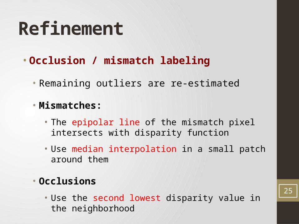
Refinement
25
• Occlusion / mismatch labeling
• Remaining outliers are re-estimated
• Mismatches:
• The epipolar line of the mismatch pixel intersects with disparity function
• Use median interpolation in a small patch around them
• Occlusions
• Use the second lowest disparity value in the neighborhood

Refinement
26
• Epipolar Line
Before After

Refinement
27
• Sub-pixel estimation
• Estimation at the sub-pixel level is made by interpolating a 2nd order curve to the cost volume C(d).
• This curve is defined by the disparities of the preceding and following pixels and their corresponding cost values
• Choose minimum cost position through a closed form solution for the 3 curve points.

Refinement
28
• Disparity map smoothing
• Median filter is applied.
The effect of overall post-processing refinement

ExperimentalResults
29

Experimental Results
• Evaluated on the Middlebury and EPFL multi-view datasets
• Parameter values were kept constant for all tests.
30

31

Experimental Results• Middlebury evaluation
32
Error Threshold = 1
Error Threshold = 0.75
33
[13] method
Proposed Method

Experimental Results
34
A Initial disparity map D Remaining occlusion/ mismatch handling
B Cost smoothing E Sub-pixel estimation
C Outlier filtering F Median smoothing
Threshold = 0.75 , % of wrong pixels

Experimental Results
35
Herz-Jesu-K7 stereo pair

Experimental Results
36
Herz-Jesu-K7 stereo pair

Conclusion
37

Conclusion
38
Initial Cost • AD (color / gradient)• Census (color / gradient)
Aggregation • Aggregation more times• Normalize → Smoothing
Refinement• Mismatch : Epipolar Line / Interpolation• Sub-pixel Estimation• Occlusion / Parameter adjustment


