January 12, 2006 14:18 01477
Tutorials and Reviews
International Journal of Bifurcation and Chaos, Vol. 15, No. 12 (2005) 3701–3849c© World Scientific Publishing Company
A NONLINEAR DYNAMICS PERSPECTIVEOF WOLFRAM’S NEW KIND OF SCIENCE.
PART V: FRACTALS EVERYWHERE
LEON O. CHUA, VALERY I. SBITNEV and SOOK YOONDepartment of Electrical Engineering and Computer Sciences,
University of California at Berkeley, CA 94720, USA
Received April 5, 2005; Revised July 10, 2005
This fifth installment is devoted to an in-depth study of CA Characteristic Functions, a unifiedglobal representation for all 256 one-dimensional Cellular Automata local rules. Except for eightrather special local rules whose global dynamics are described by an affine (mod 1 ) function ofonly one binary cell state variable, all characteristic functions exhibit a fractal geometry whereself-similar two-dimensional substructures manifest themselves, ad infinitum, as the number ofcells (I + 1) → ∞.
In addition to a complete gallery of time-1 characteristic functions for all 256 local rules,an accompanying table of explicit formulas is given for generating these characteristic functionsdirectly from binary bit-strings, as in a digital-to-analog converter. To illustrate the potentialapplications of these fundamental formulas, we prove rigorously that the “right-copycat” localrule 170 is equivalent globally to the classic “left-shift” Bernoulli map. Similarly, we prove the“left-copycat” local rule 240 is equivalent globally to the “right-shift” inverse Bernoulli map.
Various geometrical and analytical properties have been identified from each characteristicfunction and explained rigorously. In particular, two-level stratified subpatterns found in mostcharacteristic functions are shown to emerge if, and only if, b1 �= 0, where b1 is the “synapticcoefficient” associated with the cell differential equation developed in Part I.
Gardens of Eden are derived from the decimal range of the characteristic function of eachlocal rule and tabulated. Each of these binary strings has no predecessors (pre-image) and hastherefore no past, but only the present and the future. Even more fascinating, many local rulesare endowed with binary configurations which not only have no predecessors, but are also fixedpoints of the characteristic functions. To dramatize that such points have no past, and no future,they are henceforth christened “Isles of Eden”. They too have been identified and tabulated.
Keywords : Cellular neural networks, CNN; cellular automata; Turing machine; universal com-putation; Bernoulli shift; 1/f power spectrum; global equivalence classes attractors; invariantorbits; Garden of Eden; Isle of Eden; characteristic function; fractal geometry; fractals.
1. Characteristic Functions: GlobalRepresentation of Local Rules
The fundamental concept of the time-1 character-istic function
χ1N : [0, 1] → [0, 1] (1)
of a local rule N is defined in Part IV [Chua et al.,2005] as a function from the unit interval [0, 1] into
itself which uniquely maps each input binary string{x0, x1, x2, . . . , xI} represented in decimal form
φ =I∑
i=0
2−(i+1)xi (2)
into an output binary string
χ1N (φ) =
I∑i=0
2−(i+1)yi (3)
3701

January 12, 2006 14:18 01477
3702 L. O. Chua et al.
Cell(I-1)
Cell(I-2) Cell
ICell
0Cell
1Cell
2
Cell(i-1)
Celli
Cell(i+1)
1tiu −tiu
1tiu +
Local1
outputtiu +
input Symbolic Truth Table
1117
0116
1015
0014
1103
0102
1001
0000 0β
1β2β
3β
4β
5β6β7β
11 1( , , )
t t t ti i i iu u uu +
− += N
1117
-1116
1-115
-1-114
11-13
-11-12
1-1-11
-1-1-10 0γ1γ2γ3γ4γ
5γ6γ
7γ
RuleN
Numeric Truth Table
1tiu −
tiu 1
tiu +
1tiu +
1tiu −
tiu 1
tiu +
1tiu +
4
6 7
5
1
32
0 21 = 2
27 = 12826 = 64
22 = 4 23 = 8
24 = 16
20 = 1
25 = 32(1,-1,1)
(-1,-1,1)
(1,1,1)
(-1,1,1)(-1,1,-1)
(1,1,-1)
(-1,-1,-1)
(1,-1,-1)
1tiu
1tiu
tiu
4
6 7
5
1
32
0 21 = 2
27 = 12826 = 64
22 = 4 23 = 8
24 = 16
20 = 1
25 = 32(1,-1,1)
(-1,-1,1)
(1,1,1)
(-1,1,1)(-1,1,-1)
(1,1,-1)
(-1,-1,-1)
(1,-1,-1)
−
+
tiu
Fig. 1. (a) A one-dimensional Cellular Automata (CA) made of (I + 1) identical cells with a periodic boundary condition.Each cell “i” is coupled only to its left neighbor cell (i − 1) and right neighbor cell (i + 1). (b) Each cell “i” is described by alocal rule N , where N is a decimal number specified by a binary string {β0, β1, . . . , β7}, βi ∈ {0, 1}. (c) The symbolic truthtable specifying each local rule N , N = 0, 1, 2, . . . , 255. (d) By recoding “0” to “−1”, each row of the symbolic truth tablein (c) can be recast into a numeric truth table, where γk ∈ {−1, 1}. (e) Each row of the numeric truth table in (d) can berepresented as a vertex of a Boolean Cube whose color is red if γk = 1, and blue if γk = −1.

January 12, 2006 14:18 01477
A Nonlinear Dynamics Perspective of Wolfram’s New Kind of Science. Part V 3703
NT
ΣΦ Φ
[ ]0, 1 [ ]0, 11
Nχ
Σ
Fig. 2. A commutative diagram establishing a one-to-onecorrespondence between TN and χ1
N.
in decimal representation, as I → ∞, where{y0, y1, y2, . . . , yI} is the output binary string deter-mined from the local rule N of the one-dimensionalcellular automata under a periodic boundary con-dition, as shown in Fig. 1. Every input binarystring is assumed to be finite but whose lengthcan be chosen to be arbitrarily large. For prac-tical calculation, the domain of the characteristicfunction χ1
Nconsists of only a large but finite
number of equally-spaced real numbers inside [0, 1].In the limit I → ∞, the domain of χ1
Ncoin-
cides with the entire unit interval [0, 1]. In thiscase, every point φ ∈ [0, 1] corresponds uniquelyto an infinite binary string. Conversely, each infi-nite binary string corresponds to a unique pointon [0, 1]. This one-to-one correspondence betweeneach binary string in the set Σ of all infinite binarystrings and each real number in [0, 1] is depictedin Fig. 2, where φ is defined via Eq. (2). Observethat since the time-1 characteristic function χ1
N
maps each infinite binary string into anotherinfinite binary string after one iteration of the localrule N , it is a global representation.1
1.1. Deriving explicit formula forcalculating χ1
N
Recall from Eq. (8) of [Chua et al., 2004] that theoutput of each local rule N can be calculated fromthe formula
(4)
where the eight parameters {z2, c2, z1, c1, z0, b1,b2, b3} determining each local rule N is given in
Table 4 of [Chua et al., 2003]. Since χ1N
is definedin terms of binary variables xi ∈ {0, 1}, let us applythe conversion relationship Eq. (4) from [Chuaet al., 2005] namely,
xi =12
(ui + 1) (5)
and define the step function
(6)
to rewrite Eq. (4) into
(7)
where
z′0 � 12[z0 − (b1 + b2 + b3)]
z′1 � 12z1
z′2 � 12z2
(8)
Substituting Eq. (7) for yi = xt+1i in Eq. (3),
and deleting the superscripts, we obtain the fol-lowing explicit formula for calculating the charac-teristic function χ1
Nfor any local rule N , N =
0, 1, 2, . . . , 255:
(9)
where {z′2, c2, z′1, c1, z
′0, b1, b2, b3} are defined in
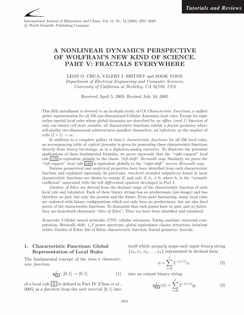
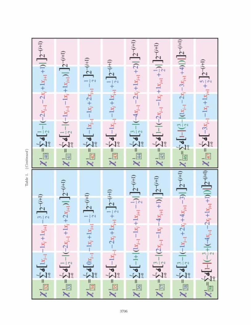
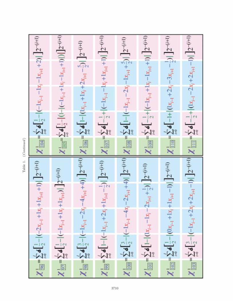
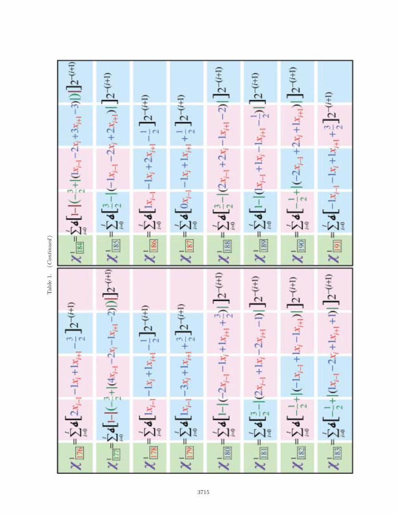
Eq. (8) and Table 4 of [Chua et al., 2003].Applying Eq. (9) to all 256 local rules, we
obtain the explicit formulas listed in Table 1 forcalculating the corresponding time-1 characteris-tic functions χ1
N, N = 0, 1, 2, . . . , 255, where the
binary string begins from φ = 0 corresponding to
{0, 0, 0, · · · 0},↑ ↑ ↑ ↑x0 x1 x2 xI
1We can define a time-k characteristic function χkN
: [0, 1] → [0, 1] in exactly the same way where the output string is
calculated after every “k” iterations under rule N .

January12,
200614:18
01477
Table 1. Explicit formulas for calculating characteristic functions χ1N
in terms of binary strings {x0, x1, x2, . . . , xI}. Each row is partitioned into four equal parts,
where each part is color coded either in blue, if the characteristic function has no stratification (see Tables 2 and 5), or in pink, otherwise.
3704

January 12, 2006 14:18 01477
Table
1.
(Continued
)
3705
January 12, 2006 14:18 01477
Table
1.
(Continued
)
3706

January 12, 2006 14:18 01477
Table
1.
(Continued
)
3707

January 12, 2006 14:18 01477
Table
1.
(Continued
)
3708

January 12, 2006 14:18 01477
Table
1.
(Continued
)
3709
January 12, 2006 14:18 01477
Table
1.
(Continued
)
3710

January 12, 2006 14:18 01477
Table
1.
(Continued
)
3711

January 12, 2006 14:18 01477
Table
1.
(Continued
)
3712

January 12, 2006 14:18 01477
Table
1.
(Continued
)
3713

January 12, 2006 14:18 01477
Table
1.
(Continued
)
3714
January 12, 2006 14:18 01477
Table
1.
(Continued
)
3715

January 12, 2006 14:18 01477
Table
1.
(Continued
)
3716

January 12, 2006 14:18 01477
Table
1.
(Continued
)
3717

January 12, 2006 14:18 01477
Table
1.
(Continued
)
3718

January 12, 2006 14:18 01477
Table
1.
(Continued
)
3719

January 12, 2006 14:18 01477
3720 L. O. Chua et al.
to φ = 1 corresponding to
{1, 1, 1, · · · 1}.↑ ↑ ↑ ↑x0 x1 x2 xI
1.2. Graphs of characteristicfunctions χ1
N
For future reference, we have plotted the time-1 characteristic functions χ1
Nfor all 256 local
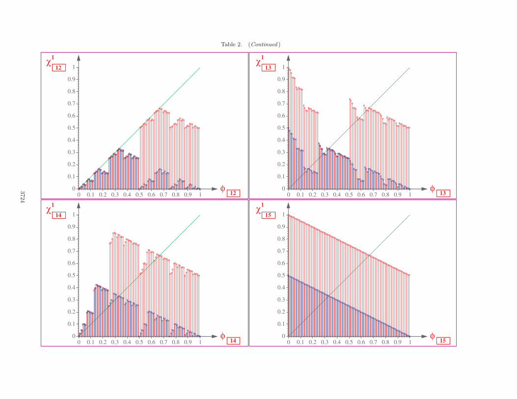
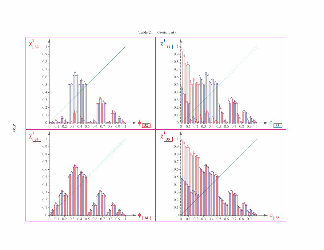
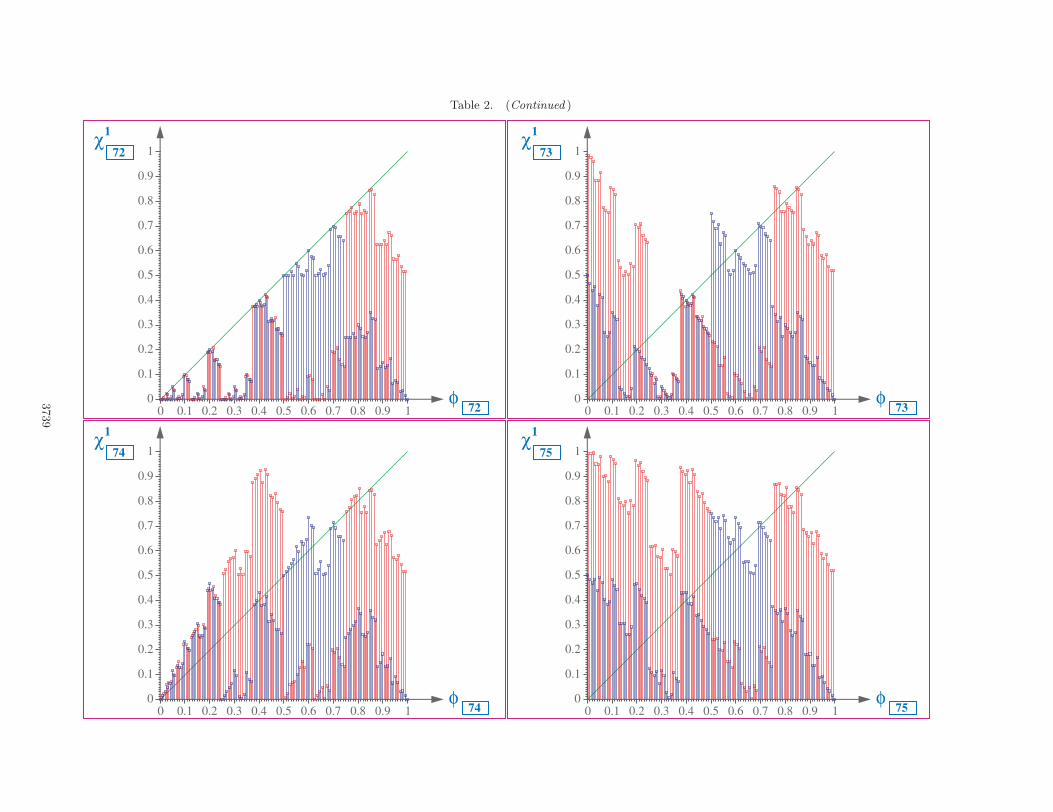
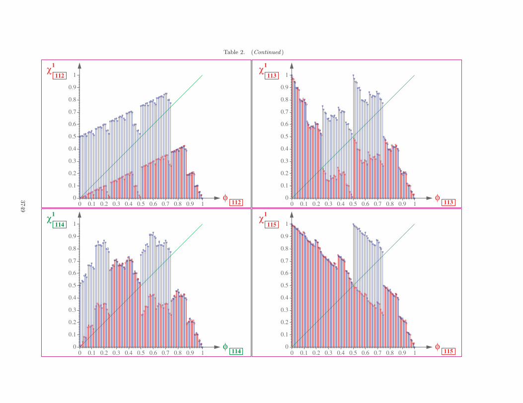
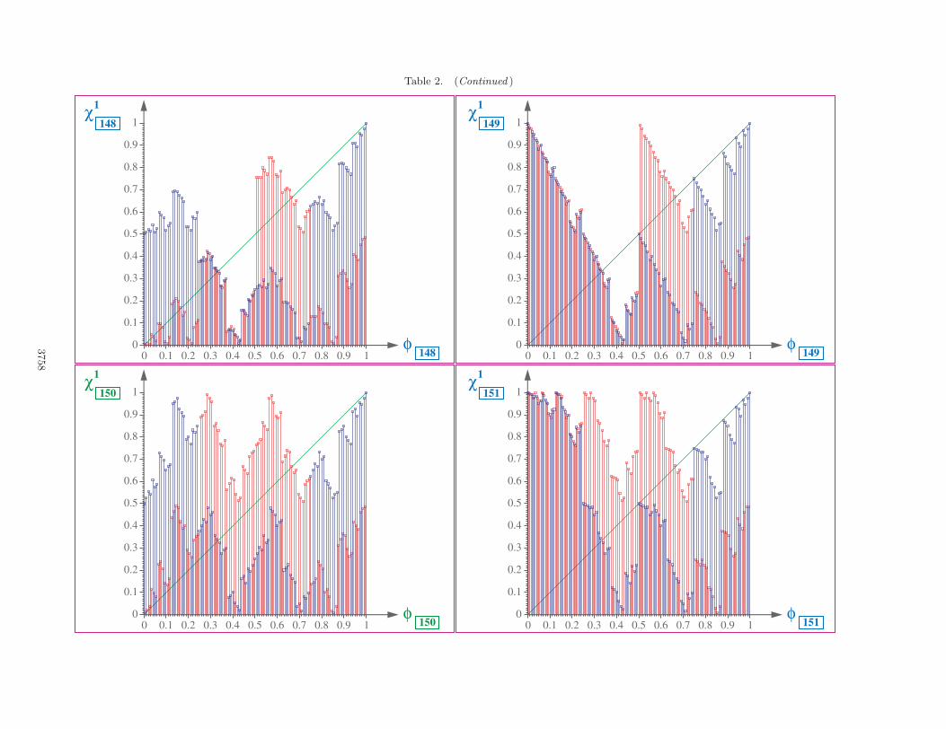
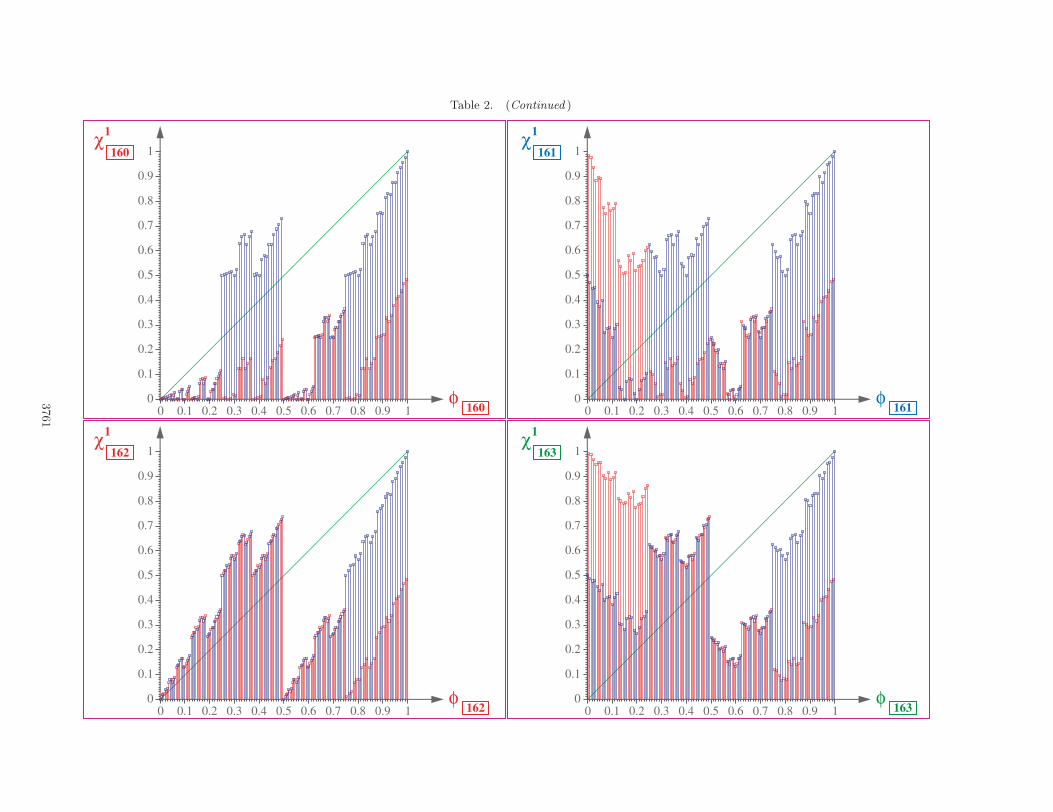
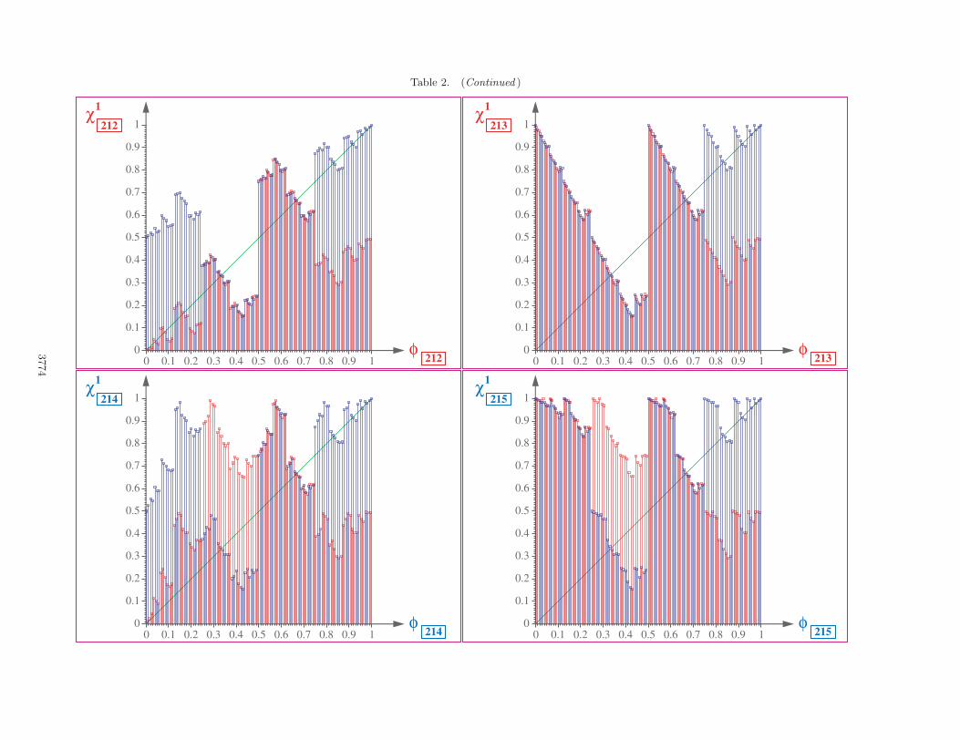
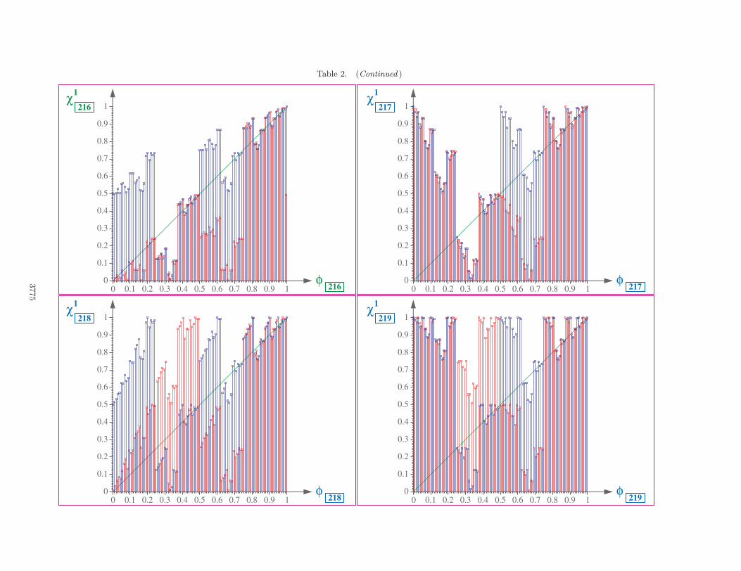
rules with I = 65, and displayed them in Table 2showing only 201 points for each rule to avoid clut-ter. In other words, each graph of χ1
Nin Table 2
shows only 201 values of χ1N
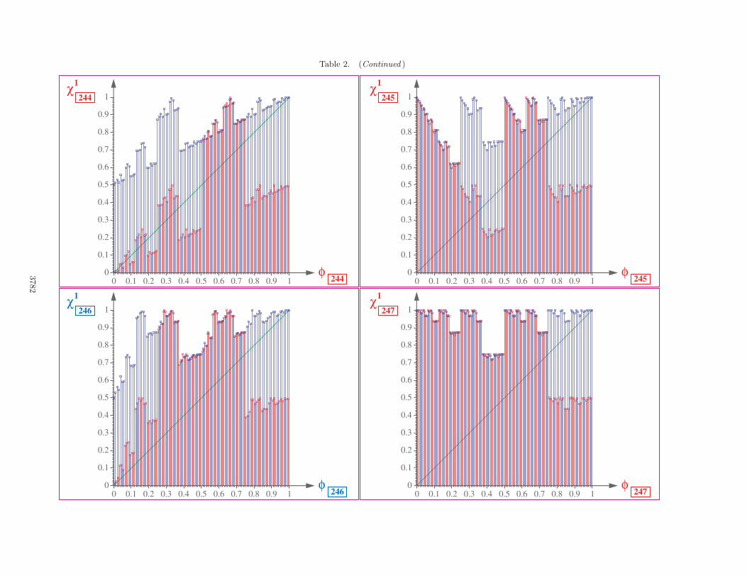
, each one calcu-lated from a 66-bit binary string. To enhance clar-ity, every pair of adjacent points in each graphare plotted as a small “red” square “ ” anda small “blue” square “ ” on top of alternat-ing red and blue color bars emanating from eachvalue of φ ∈ [0, 1] corresponding to the 201uniformly distributed points with spacing ∆φ =0.005.
A careful examination of Table 2 reveals thatadjacent pairs of points of χ1
Nare either loca-
ted in “close proximity” of each other, or theyexhibit an “abrupt jump” from each other. We willhenceforth refer to those subintervals where adja-cent red and blue squares are close to each other as“smooth”, and those exhibiting “abrupt jumps” as“discontinuous”. A careful analysis of these subin-tervals reveal that they extend over a minimumrange of ∆φ = 0.25 for all 256 rules. For exam-ple, only the second subinterval φ ∈ [0.25, 0.50) ofrule 2 is discontinuous. On the other hand, the firstand second subintervals [0, 0.25) and [0.25, 0.50) ofrule 3 are discontinuous. For rule 110 , we findonly the fourth subinterval [0.75, 1.00] is discontin-uous. For rule 30 , we find all four subintervals[0, 0.25), [0.25, 0.50), [0.50, 0.75) and [0.75, 1.00) arediscontinuous. Since these properties are quite use-ful for understanding the global dynamics of localrules, we have divided the area to the right ofthe equality sign of each characteristic functionχ1
Nin Table 1 into the above four corresponding
equal parts, and painted each part with a light bluebackground color if the corresponding subintervalhas smooth adjacent red and blue squares, or ina light pink background color if adjacent red andblue squares exhibit discontinuous jumps from eachother.
1.3. Deriving the Bernoulli mapfrom χ1
170
As an application of the explicit formulas listedin Table 1, let us apply the characteristic func-tion χ1
170of 170 to an (I + 1)-bit binary string
{x0, x1, x2, . . . , xI} with decimal representation
φ =I∑
i=0
2−(i+1)xi (10)
to obtain
χ1170 (φ) =
I∑i=0
2−(i+1)xi+1 =I+1∑j=1
2−jxj + x0 − x0
= 2
[I+1∑j=0
2−(j+1)xj
]− x0
={
2φ, φ < 0.52φ − 1, φ ≥ 0.5
(11)
as I → ∞.It follows from Eq. (11) that the characteris-
tic function χ1170
of the rule 170 converges to thewell-known Bernoulli map [Billingsley, 1978]
χ1170
(φ) = 2φ mod1 (12)
as I → ∞.Since the output of each pixel “i” of rule 170
in Table 1 is given simply by yi = xi+1, the localrule 170 consists of simply copying the “state” ofthe pixel “i + 1” of the right-neighboring pixel. Wewill henceforth call rule 170 the right-copycat rule.The graph of the right-copycat rule 170 is shownin Fig. 3.
1.4. Deriving inverse Bernoullimap from χ1
240
Let us apply the characteristic function χ1240
of240 from Table 1 to the (I + 1)-bit binary string φdefined in Eq. (10) to obtain
χ1240 (φ) =
I∑i=0
2−(i+1)xi−1 =12
I−1∑j=−1
2−(j+1)xj
=12
[I−1∑j=0
2−(j+1)xj
]+
12xI
=12φ +
12xI (13)
as I → ∞.

January12,
200614:18
01477
Table 2. Gallery of characteristic functions.
0 0.1 0.2 0.3 0.4 0.5 0.6 0.7 0.8 0.9 10
0.1
0.2
0.3
0.4
0.5
0.6
0.7
0.8
0.9
1
φ
χ1
1
1
0 0.1 0.2 0.3 0.4 0.5 0.6 0.7 0.8 0.9 10
0.1
0.2
0.3
0.4
0.5
0.6
0.7
0.8
0.9
1
φ
χ1
3
3
0 0.1 0.2 0.3 0.4 0.5 0.6 0.7 0.8 0.9 10
0.1
0.2
0.3
0.4
0.5
0.6
0.7
0.8
0.9
1
φ
χ1
0
0
0 0.1 0.2 0.3 0.4 0.5 0.6 0.7 0.8 0.9 10
0.1
0.2
0.3
0.4
0.5
0.6
0.7
0.8
0.9
1
φ
χ1
2
2
3721

January12,
200614:18
01477
Table 2. (Continued )
0 0.1 0.2 0.3 0.4 0.5 0.6 0.7 0.8 0.9 10
0.1
0.2
0.3
0.4
0.5
0.6
0.7
0.8
0.9
1
φ
χ1
5
5
0 0.1 0.2 0.3 0.4 0.5 0.6 0.7 0.8 0.9 10
0.1
0.2
0.3
0.4
0.5
0.6
0.7
0.8
0.9
1
φ
χ1
7
7
0 0.1 0.2 0.3 0.4 0.5 0.6 0.7 0.8 0.9 10
0.1
0.2
0.3
0.4
0.5
0.6
0.7
0.8
0.9
1
φ
χ1
4
4
0 0.1 0.2 0.3 0.4 0.5 0.6 0.7 0.8 0.9 10
0.1
0.2
0.3
0.4
0.5
0.6
0.7
0.8
0.9
1
φ
χ1
6
6
3722

January12,
200614:18
01477
Table 2. (Continued )
0 0.1 0.2 0.3 0.4 0.5 0.6 0.7 0.8 0.9 10
0.1
0.2
0.3
0.4
0.5
0.6
0.7
0.8
0.9
1
φ
χ1
9
9
0 0.1 0.2 0.3 0.4 0.5 0.6 0.7 0.8 0.9 10
0.1
0.2
0.3
0.4
0.5
0.6
0.7
0.8
0.9
1
φ
χ1
11
11
0 0.1 0.2 0.3 0.4 0.5 0.6 0.7 0.8 0.9 10
0.1
0.2
0.3
0.4
0.5
0.6
0.7
0.8
0.9
1
φ
χ1
8
8
0 0.1 0.2 0.3 0.4 0.5 0.6 0.7 0.8 0.9 10
0.1
0.2
0.3
0.4
0.5
0.6
0.7
0.8
0.9
1
φ
χ1
10
10
3723
January12,
200614:18
01477
Table 2. (Continued )
0 0.1 0.2 0.3 0.4 0.5 0.6 0.7 0.8 0.9 10
0.1
0.2
0.3
0.4
0.5
0.6
0.7
0.8
0.9
1
φ
χ1
13
13
0 0.1 0.2 0.3 0.4 0.5 0.6 0.7 0.8 0.9 10
0.1
0.2
0.3
0.4
0.5
0.6
0.7
0.8
0.9
1
φ
χ1
15
15
0 0.1 0.2 0.3 0.4 0.5 0.6 0.7 0.8 0.9 10
0.1
0.2
0.3
0.4
0.5
0.6
0.7
0.8
0.9
1
φ
χ1
12
12
0 0.1 0.2 0.3 0.4 0.5 0.6 0.7 0.8 0.9 10
0.1
0.2
0.3
0.4
0.5
0.6
0.7
0.8
0.9
1
φ
χ1
14
14
3724

January12,
200614:18
01477
Table 2. (Continued )
0 0.1 0.2 0.3 0.4 0.5 0.6 0.7 0.8 0.9 10
0.1
0.2
0.3
0.4
0.5
0.6
0.7
0.8
0.9
1
φ
χ1
17
17
0 0.1 0.2 0.3 0.4 0.5 0.6 0.7 0.8 0.9 10
0.1
0.2
0.3
0.4
0.5
0.6
0.7
0.8
0.9
1
φ
χ1
19
19
0 0.1 0.2 0.3 0.4 0.5 0.6 0.7 0.8 0.9 10
0.1
0.2
0.3
0.4
0.5
0.6
0.7
0.8
0.9
1
φ
χ1
16
16
0 0.1 0.2 0.3 0.4 0.5 0.6 0.7 0.8 0.9 10
0.1
0.2
0.3
0.4
0.5
0.6
0.7
0.8
0.9
1
φ
χ1
18
18
3725

January12,
200614:18
01477
Table 2. (Continued )
0 0.1 0.2 0.3 0.4 0.5 0.6 0.7 0.8 0.9 10
0.1
0.2
0.3
0.4
0.5
0.6
0.7
0.8
0.9
1
φ
χ1
21
21
0 0.1 0.2 0.3 0.4 0.5 0.6 0.7 0.8 0.9 10
0.1
0.2
0.3
0.4
0.5
0.6
0.7
0.8
0.9
1
φ
χ1
23
23
0 0.1 0.2 0.3 0.4 0.5 0.6 0.7 0.8 0.9 10
0.1
0.2
0.3
0.4
0.5
0.6
0.7
0.8
0.9
1
φ
χ1
20
20
0 0.1 0.2 0.3 0.4 0.5 0.6 0.7 0.8 0.9 10
0.1
0.2
0.3
0.4
0.5
0.6
0.7
0.8
0.9
1
φ
χ1
22
22
3726

January12,
200614:18
01477
Table 2. (Continued )
0 0.1 0.2 0.3 0.4 0.5 0.6 0.7 0.8 0.9 10
0.1
0.2
0.3
0.4
0.5
0.6
0.7
0.8
0.9
1
φ
χ1
25
25
0 0.1 0.2 0.3 0.4 0.5 0.6 0.7 0.8 0.9 10
0.1
0.2
0.3
0.4
0.5
0.6
0.7
0.8
0.9
1
φ
χ1
27
27
0 0.1 0.2 0.3 0.4 0.5 0.6 0.7 0.8 0.9 10
0.1
0.2
0.3
0.4
0.5
0.6
0.7
0.8
0.9
1
φ
χ1
24
24
0 0.1 0.2 0.3 0.4 0.5 0.6 0.7 0.8 0.9 10
0.1
0.2
0.3
0.4
0.5
0.6
0.7
0.8
0.9
1
φ
χ1
26
26
3727

January12,
200614:18
01477
Table 2. (Continued )
0 0.1 0.2 0.3 0.4 0.5 0.6 0.7 0.8 0.9 10
0.1
0.2
0.3
0.4
0.5
0.6
0.7
0.8
0.9
1
φ
χ1
29
29
0 0.1 0.2 0.3 0.4 0.5 0.6 0.7 0.8 0.9 10
0.1
0.2
0.3
0.4
0.5
0.6
0.7
0.8
0.9
1
φ
χ1
31
31
0 0.1 0.2 0.3 0.4 0.5 0.6 0.7 0.8 0.9 10
0.1
0.2
0.3
0.4
0.5
0.6
0.7
0.8
0.9
1
φ
χ1
28
28
0 0.1 0.2 0.3 0.4 0.5 0.6 0.7 0.8 0.9 10
0.1
0.2
0.3
0.4
0.5
0.6
0.7
0.8
0.9
1
φ
χ1
30
30
3728
January12,
200614:18
01477
Table 2. (Continued )
0 0.1 0.2 0.3 0.4 0.5 0.6 0.7 0.8 0.9 10
0.1
0.2
0.3
0.4
0.5
0.6
0.7
0.8
0.9
1
φ
χ1
33
33
0 0.1 0.2 0.3 0.4 0.5 0.6 0.7 0.8 0.9 10
0.1
0.2
0.3
0.4
0.5
0.6
0.7
0.8
0.9
1
φ
χ1
35
35
0 0.1 0.2 0.3 0.4 0.5 0.6 0.7 0.8 0.9 10
0.1
0.2
0.3
0.4
0.5
0.6
0.7
0.8
0.9
1
φ
χ1
32
32
0 0.1 0.2 0.3 0.4 0.5 0.6 0.7 0.8 0.9 10
0.1
0.2
0.3
0.4
0.5
0.6
0.7
0.8
0.9
1
φ
χ1
34
34
3729

January12,
200614:18
01477
Table 2. (Continued )
0 0.1 0.2 0.3 0.4 0.5 0.6 0.7 0.8 0.9 10
0.1
0.2
0.3
0.4
0.5
0.6
0.7
0.8
0.9
1
φ
χ1
37
37
0 0.1 0.2 0.3 0.4 0.5 0.6 0.7 0.8 0.9 10
0.1
0.2
0.3
0.4
0.5
0.6
0.7
0.8
0.9
1
φ
χ1
39
39
0 0.1 0.2 0.3 0.4 0.5 0.6 0.7 0.8 0.9 10
0.1
0.2
0.3
0.4
0.5
0.6
0.7
0.8
0.9
1
φ
χ1
36
36
0 0.1 0.2 0.3 0.4 0.5 0.6 0.7 0.8 0.9 10
0.1
0.2
0.3
0.4
0.5
0.6
0.7
0.8
0.9
1
φ
χ1
38
38
3730

January12,
200614:18
01477
Table 2. (Continued )
0 0.1 0.2 0.3 0.4 0.5 0.6 0.7 0.8 0.9 10
0.1
0.2
0.3
0.4
0.5
0.6
0.7
0.8
0.9
1
φ
χ1
41
41
0 0.1 0.2 0.3 0.4 0.5 0.6 0.7 0.8 0.9 10
0.1
0.2
0.3
0.4
0.5
0.6
0.7
0.8
0.9
1
φ
χ1
43
43
0 0.1 0.2 0.3 0.4 0.5 0.6 0.7 0.8 0.9 10
0.1
0.2
0.3
0.4
0.5
0.6
0.7
0.8
0.9
1
φ
χ1
40
40
0 0.1 0.2 0.3 0.4 0.5 0.6 0.7 0.8 0.9 10
0.1
0.2
0.3
0.4
0.5
0.6
0.7
0.8
0.9
1
φ
χ1
42
42
3731

January12,
200614:18
01477
Table 2. (Continued )
0 0.1 0.2 0.3 0.4 0.5 0.6 0.7 0.8 0.9 10
0.1
0.2
0.3
0.4
0.5
0.6
0.7
0.8
0.9
1
φ
χ1
45
45
0 0.1 0.2 0.3 0.4 0.5 0.6 0.7 0.8 0.9 10
0.1
0.2
0.3
0.4
0.5
0.6
0.7
0.8
0.9
1
φ
χ1
47
47
0 0.1 0.2 0.3 0.4 0.5 0.6 0.7 0.8 0.9 10
0.1
0.2
0.3
0.4
0.5
0.6
0.7
0.8
0.9
1
φ
χ1
44
44
0 0.1 0.2 0.3 0.4 0.5 0.6 0.7 0.8 0.9 10
0.1
0.2
0.3
0.4
0.5
0.6
0.7
0.8
0.9
1
φ
χ1
46
46
3732

January12,
200614:18
01477
Table 2. (Continued )
0 0.1 0.2 0.3 0.4 0.5 0.6 0.7 0.8 0.9 10
0.1
0.2
0.3
0.4
0.5
0.6
0.7
0.8
0.9
1
φ
χ1
49
49
0 0.1 0.2 0.3 0.4 0.5 0.6 0.7 0.8 0.9 10
0.1
0.2
0.3
0.4
0.5
0.6
0.7
0.8
0.9
1
φ
χ1
51
51
0 0.1 0.2 0.3 0.4 0.5 0.6 0.7 0.8 0.9 10
0.1
0.2
0.3
0.4
0.5
0.6
0.7
0.8
0.9
1
φ
χ1
48
48
0 0.1 0.2 0.3 0.4 0.5 0.6 0.7 0.8 0.9 10
0.1
0.2
0.3
0.4
0.5
0.6
0.7
0.8
0.9
1
φ
χ1
50
50
3733

January12,
200614:18
01477
Table 2. (Continued )
0 0.1 0.2 0.3 0.4 0.5 0.6 0.7 0.8 0.9 10
0.1
0.2
0.3
0.4
0.5
0.6
0.7
0.8
0.9
1
φ
χ1
53
53
0 0.1 0.2 0.3 0.4 0.5 0.6 0.7 0.8 0.9 10
0.1
0.2
0.3
0.4
0.5
0.6
0.7
0.8
0.9
1
φ
χ1
55
55
0 0.1 0.2 0.3 0.4 0.5 0.6 0.7 0.8 0.9 10
0.1
0.2
0.3
0.4
0.5
0.6
0.7
0.8
0.9
1
φ
χ1
52
52
0 0.1 0.2 0.3 0.4 0.5 0.6 0.7 0.8 0.9 10
0.1
0.2
0.3
0.4
0.5
0.6
0.7
0.8
0.9
1
φ
χ1
54
54
3734

January12,
200614:18
01477
Table 2. (Continued )
0 0.1 0.2 0.3 0.4 0.5 0.6 0.7 0.8 0.9 10
0.1
0.2
0.3
0.4
0.5
0.6
0.7
0.8
0.9
1
φ
χ1
57
57
0 0.1 0.2 0.3 0.4 0.5 0.6 0.7 0.8 0.9 10
0.1
0.2
0.3
0.4
0.5
0.6
0.7
0.8
0.9
1
φ
χ1
59
59
0 0.1 0.2 0.3 0.4 0.5 0.6 0.7 0.8 0.9 10
0.1
0.2
0.3
0.4
0.5
0.6
0.7
0.8
0.9
1
φ
χ1
56
56
0 0.1 0.2 0.3 0.4 0.5 0.6 0.7 0.8 0.9 10
0.1
0.2
0.3
0.4
0.5
0.6
0.7
0.8
0.9
1
φ
χ1
58
58
3735

January12,
200614:18
01477
Table 2. (Continued )
0 0.1 0.2 0.3 0.4 0.5 0.6 0.7 0.8 0.9 10
0.1
0.2
0.3
0.4
0.5
0.6
0.7
0.8
0.9
1
φ
χ1
61
61
0 0.1 0.2 0.3 0.4 0.5 0.6 0.7 0.8 0.9 10
0.1
0.2
0.3
0.4
0.5
0.6
0.7
0.8
0.9
1
φ
χ1
63
63
0 0.1 0.2 0.3 0.4 0.5 0.6 0.7 0.8 0.9 10
0.1
0.2
0.3
0.4
0.5
0.6
0.7
0.8
0.9
1
φ
χ1
60
60
0 0.1 0.2 0.3 0.4 0.5 0.6 0.7 0.8 0.9 10
0.1
0.2
0.3
0.4
0.5
0.6
0.7
0.8
0.9
1
φ
χ1
62
62
3736

January12,
200614:18
01477
Table 2. (Continued )
0 0.1 0.2 0.3 0.4 0.5 0.6 0.7 0.8 0.9 10
0.1
0.2
0.3
0.4
0.5
0.6
0.7
0.8
0.9
1
φ
χ1
65
65
0 0.1 0.2 0.3 0.4 0.5 0.6 0.7 0.8 0.9 10
0.1
0.2
0.3
0.4
0.5
0.6
0.7
0.8
0.9
1
φ
χ1
67
67
0 0.1 0.2 0.3 0.4 0.5 0.6 0.7 0.8 0.9 10
0.1
0.2
0.3
0.4
0.5
0.6
0.7
0.8
0.9
1
φ
χ1
64
64
0 0.1 0.2 0.3 0.4 0.5 0.6 0.7 0.8 0.9 10
0.1
0.2
0.3
0.4
0.5
0.6
0.7
0.8
0.9
1
φ
χ1
66
66
3737

January12,
200614:18
01477
Table 2. (Continued )
0 0.1 0.2 0.3 0.4 0.5 0.6 0.7 0.8 0.9 10
0.1
0.2
0.3
0.4
0.5
0.6
0.7
0.8
0.9
1
φ
χ1
69
69
0 0.1 0.2 0.3 0.4 0.5 0.6 0.7 0.8 0.9 10
0.1
0.2
0.3
0.4
0.5
0.6
0.7
0.8
0.9
1
φ
χ1
71
71
0 0.1 0.2 0.3 0.4 0.5 0.6 0.7 0.8 0.9 10
0.1
0.2
0.3
0.4
0.5
0.6
0.7
0.8
0.9
1
φ
χ1
68
68
0 0.1 0.2 0.3 0.4 0.5 0.6 0.7 0.8 0.9 10
0.1
0.2
0.3
0.4
0.5
0.6
0.7
0.8
0.9
1
φ
χ1
70
70
3738
January12,
200614:18
01477
Table 2. (Continued )
0 0.1 0.2 0.3 0.4 0.5 0.6 0.7 0.8 0.9 10
0.1
0.2
0.3
0.4
0.5
0.6
0.7
0.8
0.9
1
φ
χ1
73
73
0 0.1 0.2 0.3 0.4 0.5 0.6 0.7 0.8 0.9 10
0.1
0.2
0.3
0.4
0.5
0.6
0.7
0.8
0.9
1
φ
χ1
75
75
0 0.1 0.2 0.3 0.4 0.5 0.6 0.7 0.8 0.9 10
0.1
0.2
0.3
0.4
0.5
0.6
0.7
0.8
0.9
1
φ
χ1
72
72
0 0.1 0.2 0.3 0.4 0.5 0.6 0.7 0.8 0.9 10
0.1
0.2
0.3
0.4
0.5
0.6
0.7
0.8
0.9
1
φ
χ1
74
74
3739

January12,
200614:18
01477
Table 2. (Continued )
0 0.1 0.2 0.3 0.4 0.5 0.6 0.7 0.8 0.9 10
0.1
0.2
0.3
0.4
0.5
0.6
0.7
0.8
0.9
1
φ
χ1
77
77
0 0.1 0.2 0.3 0.4 0.5 0.6 0.7 0.8 0.9 10
0.1
0.2
0.3
0.4
0.5
0.6
0.7
0.8
0.9
1
φ
χ1
79
79
0 0.1 0.2 0.3 0.4 0.5 0.6 0.7 0.8 0.9 10
0.1
0.2
0.3
0.4
0.5
0.6
0.7
0.8
0.9
1
φ
χ1
76
76
0 0.1 0.2 0.3 0.4 0.5 0.6 0.7 0.8 0.9 10
0.1
0.2
0.3
0.4
0.5
0.6
0.7
0.8
0.9
1
φ
χ1
78
78
3740

January12,
200614:18
01477
Table 2. (Continued )
0 0.1 0.2 0.3 0.4 0.5 0.6 0.7 0.8 0.9 10
0.1
0.2
0.3
0.4
0.5
0.6
0.7
0.8
0.9
1
φ
χ1
81
81
0 0.1 0.2 0.3 0.4 0.5 0.6 0.7 0.8 0.9 10
0.1
0.2
0.3
0.4
0.5
0.6
0.7
0.8
0.9
1
φ
χ1
83
83
0 0.1 0.2 0.3 0.4 0.5 0.6 0.7 0.8 0.9 10
0.1
0.2
0.3
0.4
0.5
0.6
0.7
0.8
0.9
1
φ
χ1
80
80
0 0.1 0.2 0.3 0.4 0.5 0.6 0.7 0.8 0.9 10
0.1
0.2
0.3
0.4
0.5
0.6
0.7
0.8
0.9
1
φ
χ1
82
82
3741

January12,
200614:18
01477
Table 2. (Continued )
0 0.1 0.2 0.3 0.4 0.5 0.6 0.7 0.8 0.9 10
0.1
0.2
0.3
0.4
0.5
0.6
0.7
0.8
0.9
1
φ
χ1
85
85
0 0.1 0.2 0.3 0.4 0.5 0.6 0.7 0.8 0.9 10
0.1
0.2
0.3
0.4
0.5
0.6
0.7
0.8
0.9
1
φ
χ1
87
87
0 0.1 0.2 0.3 0.4 0.5 0.6 0.7 0.8 0.9 10
0.1
0.2
0.3
0.4
0.5
0.6
0.7
0.8
0.9
1
φ
χ1
84
84
0 0.1 0.2 0.3 0.4 0.5 0.6 0.7 0.8 0.9 10
0.1
0.2
0.3
0.4
0.5
0.6
0.7
0.8
0.9
1
φ
χ1
86
86
3742

January12,
200614:18
01477
Table 2. (Continued )
0 0.1 0.2 0.3 0.4 0.5 0.6 0.7 0.8 0.9 10
0.1
0.2
0.3
0.4
0.5
0.6
0.7
0.8
0.9
1
φ
χ1
89
89
0 0.1 0.2 0.3 0.4 0.5 0.6 0.7 0.8 0.9 10
0.1
0.2
0.3
0.4
0.5
0.6
0.7
0.8
0.9
1
φ
χ1
91
91
0 0.1 0.2 0.3 0.4 0.5 0.6 0.7 0.8 0.9 10
0.1
0.2
0.3
0.4
0.5
0.6
0.7
0.8
0.9
1
φ
χ1
88
88
0 0.1 0.2 0.3 0.4 0.5 0.6 0.7 0.8 0.9 10
0.1
0.2
0.3
0.4
0.5
0.6
0.7
0.8
0.9
1
φ
χ1
90
90
3743

January12,
200614:18
01477
Table 2. (Continued )
0 0.1 0.2 0.3 0.4 0.5 0.6 0.7 0.8 0.9 10
0.1
0.2
0.3
0.4
0.5
0.6
0.7
0.8
0.9
1
φ
χ1
93
93
0 0.1 0.2 0.3 0.4 0.5 0.6 0.7 0.8 0.9 10
0.1
0.2
0.3
0.4
0.5
0.6
0.7
0.8
0.9
1
φ
χ1
95
95
0 0.1 0.2 0.3 0.4 0.5 0.6 0.7 0.8 0.9 10
0.1
0.2
0.3
0.4
0.5
0.6
0.7
0.8
0.9
1
φ
χ1
92
92
0 0.1 0.2 0.3 0.4 0.5 0.6 0.7 0.8 0.9 10
0.1
0.2
0.3
0.4
0.5
0.6
0.7
0.8
0.9
1
φ
χ1
94
94
3744

January12,
200614:18
01477
Table 2. (Continued )
0 0.1 0.2 0.3 0.4 0.5 0.6 0.7 0.8 0.9 10
0.1
0.2
0.3
0.4
0.5
0.6
0.7
0.8
0.9
1
φ
χ1
97
97
0 0.1 0.2 0.3 0.4 0.5 0.6 0.7 0.8 0.9 10
0.1
0.2
0.3
0.4
0.5
0.6
0.7
0.8
0.9
1
φ
χ1
99
99
0 0.1 0.2 0.3 0.4 0.5 0.6 0.7 0.8 0.9 10
0.1
0.2
0.3
0.4
0.5
0.6
0.7
0.8
0.9
1
φ
χ1
96
96
0 0.1 0.2 0.3 0.4 0.5 0.6 0.7 0.8 0.9 10
0.1
0.2
0.3
0.4
0.5
0.6
0.7
0.8
0.9
1
φ
χ1
98
98
3745

January12,
200614:18
01477
Table 2. (Continued )
0 0.1 0.2 0.3 0.4 0.5 0.6 0.7 0.8 0.9 10
0.1
0.2
0.3
0.4
0.5
0.6
0.7
0.8
0.9
1
φ
χ1
101
101
0 0.1 0.2 0.3 0.4 0.5 0.6 0.7 0.8 0.9 10
0.1
0.2
0.3
0.4
0.5
0.6
0.7
0.8
0.9
1
φ
χ1
103
103
0 0.1 0.2 0.3 0.4 0.5 0.6 0.7 0.8 0.9 10
0.1
0.2
0.3
0.4
0.5
0.6
0.7
0.8
0.9
1
φ
χ1
100
100
0 0.1 0.2 0.3 0.4 0.5 0.6 0.7 0.8 0.9 10
0.1
0.2
0.3
0.4
0.5
0.6
0.7
0.8
0.9
1
φ
χ1
102
102
3746

January12,
200614:18
01477
Table 2. (Continued )
0 0.1 0.2 0.3 0.4 0.5 0.6 0.7 0.8 0.9 10
0.1
0.2
0.3
0.4
0.5
0.6
0.7
0.8
0.9
1
φ
χ1
105
105
0 0.1 0.2 0.3 0.4 0.5 0.6 0.7 0.8 0.9 10
0.1
0.2
0.3
0.4
0.5
0.6
0.7
0.8
0.9
1
φ
χ1
107
107
0 0.1 0.2 0.3 0.4 0.5 0.6 0.7 0.8 0.9 10
0.1
0.2
0.3
0.4
0.5
0.6
0.7
0.8
0.9
1
φ
χ1
104
104
0 0.1 0.2 0.3 0.4 0.5 0.6 0.7 0.8 0.9 10
0.1
0.2
0.3
0.4
0.5
0.6
0.7
0.8
0.9
1
φ
χ1
106
106
3747

January12,
200614:18
01477
Table 2. (Continued )
0 0.1 0.2 0.3 0.4 0.5 0.6 0.7 0.8 0.9 10
0.1
0.2
0.3
0.4
0.5
0.6
0.7
0.8
0.9
1
φ
χ1
109
109
0 0.1 0.2 0.3 0.4 0.5 0.6 0.7 0.8 0.9 10
0.1
0.2
0.3
0.4
0.5
0.6
0.7
0.8
0.9
1
φ
χ1
111
111
0 0.1 0.2 0.3 0.4 0.5 0.6 0.7 0.8 0.9 10
0.1
0.2
0.3
0.4
0.5
0.6
0.7
0.8
0.9
1
φ
χ1
108
108
0 0.1 0.2 0.3 0.4 0.5 0.6 0.7 0.8 0.9 10
0.1
0.2
0.3
0.4
0.5
0.6
0.7
0.8
0.9
1
φ
χ1
110
110
3748
January12,
200614:18
01477
Table 2. (Continued )
0 0.1 0.2 0.3 0.4 0.5 0.6 0.7 0.8 0.9 10
0.1
0.2
0.3
0.4
0.5
0.6
0.7
0.8
0.9
1
φ
χ1
113
113
0 0.1 0.2 0.3 0.4 0.5 0.6 0.7 0.8 0.9 10
0.1
0.2
0.3
0.4
0.5
0.6
0.7
0.8
0.9
1
φ
χ1
115
115
0 0.1 0.2 0.3 0.4 0.5 0.6 0.7 0.8 0.9 10
0.1
0.2
0.3
0.4
0.5
0.6
0.7
0.8
0.9
1
φ
χ1
112
112
0 0.1 0.2 0.3 0.4 0.5 0.6 0.7 0.8 0.9 10
0.1
0.2
0.3
0.4
0.5
0.6
0.7
0.8
0.9
1
φ
χ1
114
114
3749

January12,
200614:18
01477
Table 2. (Continued )
0 0.1 0.2 0.3 0.4 0.5 0.6 0.7 0.8 0.9 10
0.1
0.2
0.3
0.4
0.5
0.6
0.7
0.8
0.9
1
φ
χ1
117
117
0 0.1 0.2 0.3 0.4 0.5 0.6 0.7 0.8 0.9 10
0.1
0.2
0.3
0.4
0.5
0.6
0.7
0.8
0.9
1
φ
χ1
119
119
0 0.1 0.2 0.3 0.4 0.5 0.6 0.7 0.8 0.9 10
0.1
0.2
0.3
0.4
0.5
0.6
0.7
0.8
0.9
1
φ
χ1
116
116
0 0.1 0.2 0.3 0.4 0.5 0.6 0.7 0.8 0.9 10
0.1
0.2
0.3
0.4
0.5
0.6
0.7
0.8
0.9
1
φ
χ1
118
118
3750

January12,
200614:18
01477
Table 2. (Continued )
0 0.1 0.2 0.3 0.4 0.5 0.6 0.7 0.8 0.9 10
0.1
0.2
0.3
0.4
0.5
0.6
0.7
0.8
0.9
1
φ
χ1
121
121
0 0.1 0.2 0.3 0.4 0.5 0.6 0.7 0.8 0.9 10
0.1
0.2
0.3
0.4
0.5
0.6
0.7
0.8
0.9
1
φ
χ1
123
123
0 0.1 0.2 0.3 0.4 0.5 0.6 0.7 0.8 0.9 10
0.1
0.2
0.3
0.4
0.5
0.6
0.7
0.8
0.9
1
φ
χ1
120
120
0 0.1 0.2 0.3 0.4 0.5 0.6 0.7 0.8 0.9 10
0.1
0.2
0.3
0.4
0.5
0.6
0.7
0.8
0.9
1
φ
χ1
122
122
3751

January12,
200614:18
01477
Table 2. (Continued )
0 0.1 0.2 0.3 0.4 0.5 0.6 0.7 0.8 0.9 10
0.1
0.2
0.3
0.4
0.5
0.6
0.7
0.8
0.9
1
φ
χ1
125
125
0 0.1 0.2 0.3 0.4 0.5 0.6 0.7 0.8 0.9 10
0.1
0.2
0.3
0.4
0.5
0.6
0.7
0.8
0.9
1
φ
χ1
127
127
0 0.1 0.2 0.3 0.4 0.5 0.6 0.7 0.8 0.9 10
0.1
0.2
0.3
0.4
0.5
0.6
0.7
0.8
0.9
1
φ
χ1
124
124
0 0.1 0.2 0.3 0.4 0.5 0.6 0.7 0.8 0.9 10
0.1
0.2
0.3
0.4
0.5
0.6
0.7
0.8
0.9
1
φ
χ1
126
126
3752

January12,
200614:18
01477
Table 2. (Continued )
0 0.1 0.2 0.3 0.4 0.5 0.6 0.7 0.8 0.9 10
0.1
0.2
0.3
0.4
0.5
0.6
0.7
0.8
0.9
1
φ
χ1
129
129
0 0.1 0.2 0.3 0.4 0.5 0.6 0.7 0.8 0.9 10
0.1
0.2
0.3
0.4
0.5
0.6
0.7
0.8
0.9
1
φ
χ1
131
131
0 0.1 0.2 0.3 0.4 0.5 0.6 0.7 0.8 0.9 10
0.1
0.2
0.3
0.4
0.5
0.6
0.7
0.8
0.9
1
φ
χ1
128
128
0 0.1 0.2 0.3 0.4 0.5 0.6 0.7 0.8 0.9 10
0.1
0.2
0.3
0.4
0.5
0.6
0.7
0.8
0.9
1
φ
χ1
130
130
3753

January12,
200614:18
01477
Table 2. (Continued )
0 0.1 0.2 0.3 0.4 0.5 0.6 0.7 0.8 0.9 10
0.1
0.2
0.3
0.4
0.5
0.6
0.7
0.8
0.9
1
φ
χ1
133
133
0 0.1 0.2 0.3 0.4 0.5 0.6 0.7 0.8 0.9 10
0.1
0.2
0.3
0.4
0.5
0.6
0.7
0.8
0.9
1
φ
χ1
135
135
0 0.1 0.2 0.3 0.4 0.5 0.6 0.7 0.8 0.9 10
0.1
0.2
0.3
0.4
0.5
0.6
0.7
0.8
0.9
1
φ
χ1
132
132
0 0.1 0.2 0.3 0.4 0.5 0.6 0.7 0.8 0.9 10
0.1
0.2
0.3
0.4
0.5
0.6
0.7
0.8
0.9
1
φ
χ1
134
134
3754

January12,
200614:18
01477
Table 2. (Continued )
0 0.1 0.2 0.3 0.4 0.5 0.6 0.7 0.8 0.9 10
0.1
0.2
0.3
0.4
0.5
0.6
0.7
0.8
0.9
1
φ
χ1
137
137
0 0.1 0.2 0.3 0.4 0.5 0.6 0.7 0.8 0.9 10
0.1
0.2
0.3
0.4
0.5
0.6
0.7
0.8
0.9
1
φ
χ1
139
139
0 0.1 0.2 0.3 0.4 0.5 0.6 0.7 0.8 0.9 10
0.1
0.2
0.3
0.4
0.5
0.6
0.7
0.8
0.9
1
φ
χ1
136
136
0 0.1 0.2 0.3 0.4 0.5 0.6 0.7 0.8 0.9 10
0.1
0.2
0.3
0.4
0.5
0.6
0.7
0.8
0.9
1
φ
χ1
138
138
3755

January12,
200614:18
01477
Table 2. (Continued )
0 0.1 0.2 0.3 0.4 0.5 0.6 0.7 0.8 0.9 10
0.1
0.2
0.3
0.4
0.5
0.6
0.7
0.8
0.9
1
φ
χ1
141
141
0 0.1 0.2 0.3 0.4 0.5 0.6 0.7 0.8 0.9 10
0.1
0.2
0.3
0.4
0.5
0.6
0.7
0.8
0.9
1
φ
χ1
143
143
0 0.1 0.2 0.3 0.4 0.5 0.6 0.7 0.8 0.9 10
0.1
0.2
0.3
0.4
0.5
0.6
0.7
0.8
0.9
1
φ
χ1
140
140
0 0.1 0.2 0.3 0.4 0.5 0.6 0.7 0.8 0.9 10
0.1
0.2
0.3
0.4
0.5
0.6
0.7
0.8
0.9
1
φ
χ1
142
142
3756

January12,
200614:18
01477
Table 2. (Continued )
0 0.1 0.2 0.3 0.4 0.5 0.6 0.7 0.8 0.9 10
0.1
0.2
0.3
0.4
0.5
0.6
0.7
0.8
0.9
1
φ
χ1
145
145
0 0.1 0.2 0.3 0.4 0.5 0.6 0.7 0.8 0.9 10
0.1
0.2
0.3
0.4
0.5
0.6
0.7
0.8
0.9
1
φ
χ1
147
147
0 0.1 0.2 0.3 0.4 0.5 0.6 0.7 0.8 0.9 10
0.1
0.2
0.3
0.4
0.5
0.6
0.7
0.8
0.9
1
φ
χ1
144
144
0 0.1 0.2 0.3 0.4 0.5 0.6 0.7 0.8 0.9 10
0.1
0.2
0.3
0.4
0.5
0.6
0.7
0.8
0.9
1
φ
χ1
146
146
3757
January12,
200614:18
01477
Table 2. (Continued )
0 0.1 0.2 0.3 0.4 0.5 0.6 0.7 0.8 0.9 10
0.1
0.2
0.3
0.4
0.5
0.6
0.7
0.8
0.9
1
φ
χ1
149
149
0 0.1 0.2 0.3 0.4 0.5 0.6 0.7 0.8 0.9 10
0.1
0.2
0.3
0.4
0.5
0.6
0.7
0.8
0.9
1
φ
χ1
151
151
0 0.1 0.2 0.3 0.4 0.5 0.6 0.7 0.8 0.9 10
0.1
0.2
0.3
0.4
0.5
0.6
0.7
0.8
0.9
1
φ
χ1
148
148
0 0.1 0.2 0.3 0.4 0.5 0.6 0.7 0.8 0.9 10
0.1
0.2
0.3
0.4
0.5
0.6
0.7
0.8
0.9
1
φ
χ1
150
150
3758

January12,
200614:18
01477
Table 2. (Continued )
0 0.1 0.2 0.3 0.4 0.5 0.6 0.7 0.8 0.9 10
0.1
0.2
0.3
0.4
0.5
0.6
0.7
0.8
0.9
1
φ
χ1
153
153
0 0.1 0.2 0.3 0.4 0.5 0.6 0.7 0.8 0.9 10
0.1
0.2
0.3
0.4
0.5
0.6
0.7
0.8
0.9
1
φ
χ1
155
155
0 0.1 0.2 0.3 0.4 0.5 0.6 0.7 0.8 0.9 10
0.1
0.2
0.3
0.4
0.5
0.6
0.7
0.8
0.9
1
φ
χ1
152
152
0 0.1 0.2 0.3 0.4 0.5 0.6 0.7 0.8 0.9 10
0.1
0.2
0.3
0.4
0.5
0.6
0.7
0.8
0.9
1
φ
χ1
154
154
3759

January12,
200614:18
01477
Table 2. (Continued )
0 0.1 0.2 0.3 0.4 0.5 0.6 0.7 0.8 0.9 10
0.1
0.2
0.3
0.4
0.5
0.6
0.7
0.8
0.9
1
φ
χ1
157
157
0 0.1 0.2 0.3 0.4 0.5 0.6 0.7 0.8 0.9 10
0.1
0.2
0.3
0.4
0.5
0.6
0.7
0.8
0.9
1
φ
χ1
159
159
0 0.1 0.2 0.3 0.4 0.5 0.6 0.7 0.8 0.9 10
0.1
0.2
0.3
0.4
0.5
0.6
0.7
0.8
0.9
1
φ
χ1
156
156
0 0.1 0.2 0.3 0.4 0.5 0.6 0.7 0.8 0.9 10
0.1
0.2
0.3
0.4
0.5
0.6
0.7
0.8
0.9
1
φ
χ1
158
158
3760
January12,
200614:18
01477
Table 2. (Continued )
0 0.1 0.2 0.3 0.4 0.5 0.6 0.7 0.8 0.9 10
0.1
0.2
0.3
0.4
0.5
0.6
0.7
0.8
0.9
1
φ
χ1
161
161
0 0.1 0.2 0.3 0.4 0.5 0.6 0.7 0.8 0.9 10
0.1
0.2
0.3
0.4
0.5
0.6
0.7
0.8
0.9
1
φ
χ1
163
163
0 0.1 0.2 0.3 0.4 0.5 0.6 0.7 0.8 0.9 10
0.1
0.2
0.3
0.4
0.5
0.6
0.7
0.8
0.9
1
φ
χ1
160
160
0 0.1 0.2 0.3 0.4 0.5 0.6 0.7 0.8 0.9 10
0.1
0.2
0.3
0.4
0.5
0.6
0.7
0.8
0.9
1
φ
χ1
162
162
3761

January12,
200614:18
01477
Table 2. (Continued )
0 0.1 0.2 0.3 0.4 0.5 0.6 0.7 0.8 0.9 10
0.1
0.2
0.3
0.4
0.5
0.6
0.7
0.8
0.9
1
φ
χ1
165
165
0 0.1 0.2 0.3 0.4 0.5 0.6 0.7 0.8 0.9 10
0.1
0.2
0.3
0.4
0.5
0.6
0.7
0.8
0.9
1
φ
χ1
167
167
0 0.1 0.2 0.3 0.4 0.5 0.6 0.7 0.8 0.9 10
0.1
0.2
0.3
0.4
0.5
0.6
0.7
0.8
0.9
1
φ
χ1
164
164
0 0.1 0.2 0.3 0.4 0.5 0.6 0.7 0.8 0.9 10
0.1
0.2
0.3
0.4
0.5
0.6
0.7
0.8
0.9
1
φ
χ1
166
166
3762

January12,
200614:18
01477
Table 2. (Continued )
0 0.1 0.2 0.3 0.4 0.5 0.6 0.7 0.8 0.9 10
0.1
0.2
0.3
0.4
0.5
0.6
0.7
0.8
0.9
1
φ
χ1
169
169
0 0.1 0.2 0.3 0.4 0.5 0.6 0.7 0.8 0.9 10
0.1
0.2
0.3
0.4
0.5
0.6
0.7
0.8
0.9
1
φ
χ1
171
171
0 0.1 0.2 0.3 0.4 0.5 0.6 0.7 0.8 0.9 10
0.1
0.2
0.3
0.4
0.5
0.6
0.7
0.8
0.9
1
φ
χ1
168
168
0 0.1 0.2 0.3 0.4 0.5 0.6 0.7 0.8 0.9 10
0.1
0.2
0.3
0.4
0.5
0.6
0.7
0.8
0.9
1
φ
χ1
170
170
3763

January12,
200614:18
01477
Table 2. (Continued )
0 0.1 0.2 0.3 0.4 0.5 0.6 0.7 0.8 0.9 10
0.1
0.2
0.3
0.4
0.5
0.6
0.7
0.8
0.9
1
φ
χ1
173
173
0 0.1 0.2 0.3 0.4 0.5 0.6 0.7 0.8 0.9 10
0.1
0.2
0.3
0.4
0.5
0.6
0.7
0.8
0.9
1
φ
χ1
175
175
0 0.1 0.2 0.3 0.4 0.5 0.6 0.7 0.8 0.9 10
0.1
0.2
0.3
0.4
0.5
0.6
0.7
0.8
0.9
1
φ
χ1
172
172
0 0.1 0.2 0.3 0.4 0.5 0.6 0.7 0.8 0.9 10
0.1
0.2
0.3
0.4
0.5
0.6
0.7
0.8
0.9
1
φ
χ1
174
174
3764

January12,
200614:18
01477
Table 2. (Continued )
0 0.1 0.2 0.3 0.4 0.5 0.6 0.7 0.8 0.9 10
0.1
0.2
0.3
0.4
0.5
0.6
0.7
0.8
0.9
1
φ
χ1
177
177
0 0.1 0.2 0.3 0.4 0.5 0.6 0.7 0.8 0.9 10
0.1
0.2
0.3
0.4
0.5
0.6
0.7
0.8
0.9
1
φ
χ1
179
179
0 0.1 0.2 0.3 0.4 0.5 0.6 0.7 0.8 0.9 10
0.1
0.2
0.3
0.4
0.5
0.6
0.7
0.8
0.9
1
φ
χ1
176
176
0 0.1 0.2 0.3 0.4 0.5 0.6 0.7 0.8 0.9 10
0.1
0.2
0.3
0.4
0.5
0.6
0.7
0.8
0.9
1
φ
χ1
178
178
3765

January12,
200614:18
01477
Table 2. (Continued )
0 0.1 0.2 0.3 0.4 0.5 0.6 0.7 0.8 0.9 10
0.1
0.2
0.3
0.4
0.5
0.6
0.7
0.8
0.9
1
φ
χ1
181
181
0 0.1 0.2 0.3 0.4 0.5 0.6 0.7 0.8 0.9 10
0.1
0.2
0.3
0.4
0.5
0.6
0.7
0.8
0.9
1
φ
χ1
183
183
0 0.1 0.2 0.3 0.4 0.5 0.6 0.7 0.8 0.9 10
0.1
0.2
0.3
0.4
0.5
0.6
0.7
0.8
0.9
1
φ
χ1
180
180
0 0.1 0.2 0.3 0.4 0.5 0.6 0.7 0.8 0.9 10
0.1
0.2
0.3
0.4
0.5
0.6
0.7
0.8
0.9
1
φ
χ1
182
182
3766

January12,
200614:18
01477
Table 2. (Continued )
0 0.1 0.2 0.3 0.4 0.5 0.6 0.7 0.8 0.9 10
0.1
0.2
0.3
0.4
0.5
0.6
0.7
0.8
0.9
1
φ
χ1
185
185
0 0.1 0.2 0.3 0.4 0.5 0.6 0.7 0.8 0.9 10
0.1
0.2
0.3
0.4
0.5
0.6
0.7
0.8
0.9
1
φ
χ1
187
187
0 0.1 0.2 0.3 0.4 0.5 0.6 0.7 0.8 0.9 10
0.1
0.2
0.3
0.4
0.5
0.6
0.7
0.8
0.9
1
φ
χ1
184
184
0 0.1 0.2 0.3 0.4 0.5 0.6 0.7 0.8 0.9 10
0.1
0.2
0.3
0.4
0.5
0.6
0.7
0.8
0.9
1
φ
χ1
186
186
3767

January12,
200614:18
01477
Table 2. (Continued )
0 0.1 0.2 0.3 0.4 0.5 0.6 0.7 0.8 0.9 10
0.1
0.2
0.3
0.4
0.5
0.6
0.7
0.8
0.9
1
φ
χ1
189
189
0 0.1 0.2 0.3 0.4 0.5 0.6 0.7 0.8 0.9 10
0.1
0.2
0.3
0.4
0.5
0.6
0.7
0.8
0.9
1
φ
χ1
191
191
0 0.1 0.2 0.3 0.4 0.5 0.6 0.7 0.8 0.9 10
0.1
0.2
0.3
0.4
0.5
0.6
0.7
0.8
0.9
1
φ
χ1
188
188
0 0.1 0.2 0.3 0.4 0.5 0.6 0.7 0.8 0.9 10
0.1
0.2
0.3
0.4
0.5
0.6
0.7
0.8
0.9
1
φ
χ1
190
190
3768

January12,
200614:18
01477
Table 2. (Continued )
0 0.1 0.2 0.3 0.4 0.5 0.6 0.7 0.8 0.9 10
0.1
0.2
0.3
0.4
0.5
0.6
0.7
0.8
0.9
1
φ
χ1
193
193
0 0.1 0.2 0.3 0.4 0.5 0.6 0.7 0.8 0.9 10
0.1
0.2
0.3
0.4
0.5
0.6
0.7
0.8
0.9
1
φ
χ1
195
195
0 0.1 0.2 0.3 0.4 0.5 0.6 0.7 0.8 0.9 10
0.1
0.2
0.3
0.4
0.5
0.6
0.7
0.8
0.9
1
φ
χ1
192
192
0 0.1 0.2 0.3 0.4 0.5 0.6 0.7 0.8 0.9 10
0.1
0.2
0.3
0.4
0.5
0.6
0.7
0.8
0.9
1
φ
χ1
194
194
3769

January12,
200614:18
01477
Table 2. (Continued )
0 0.1 0.2 0.3 0.4 0.5 0.6 0.7 0.8 0.9 10
0.1
0.2
0.3
0.4
0.5
0.6
0.7
0.8
0.9
1
φ
χ1
197
197
0 0.1 0.2 0.3 0.4 0.5 0.6 0.7 0.8 0.9 10
0.1
0.2
0.3
0.4
0.5
0.6
0.7
0.8
0.9
1
φ
χ1
199
199
0 0.1 0.2 0.3 0.4 0.5 0.6 0.7 0.8 0.9 10
0.1
0.2
0.3
0.4
0.5
0.6
0.7
0.8
0.9
1
φ
χ1
196
196
0 0.1 0.2 0.3 0.4 0.5 0.6 0.7 0.8 0.9 10
0.1
0.2
0.3
0.4
0.5
0.6
0.7
0.8
0.9
1
φ
χ1
198
198
3770

January12,
200614:18
01477
Table 2. (Continued )
0 0.1 0.2 0.3 0.4 0.5 0.6 0.7 0.8 0.9 10
0.1
0.2
0.3
0.4
0.5
0.6
0.7
0.8
0.9
1
φ
χ1
201
201
0 0.1 0.2 0.3 0.4 0.5 0.6 0.7 0.8 0.9 10
0.1
0.2
0.3
0.4
0.5
0.6
0.7
0.8
0.9
1
φ
χ1
203
203
0 0.1 0.2 0.3 0.4 0.5 0.6 0.7 0.8 0.9 10
0.1
0.2
0.3
0.4
0.5
0.6
0.7
0.8
0.9
1
φ
χ1
200
200
0 0.1 0.2 0.3 0.4 0.5 0.6 0.7 0.8 0.9 10
0.1
0.2
0.3
0.4
0.5
0.6
0.7
0.8
0.9
1
φ
χ1
202
202
3771

January12,
200614:18
01477
Table 2. (Continued )
0 0.1 0.2 0.3 0.4 0.5 0.6 0.7 0.8 0.9 10
0.1
0.2
0.3
0.4
0.5
0.6
0.7
0.8
0.9
1
φ
χ1
205
205
0 0.1 0.2 0.3 0.4 0.5 0.6 0.7 0.8 0.9 10
0.1
0.2
0.3
0.4
0.5
0.6
0.7
0.8
0.9
1
φ
χ1
207
207
0 0.1 0.2 0.3 0.4 0.5 0.6 0.7 0.8 0.9 10
0.1
0.2
0.3
0.4
0.5
0.6
0.7
0.8
0.9
1
φ
χ1
204
204
0 0.1 0.2 0.3 0.4 0.5 0.6 0.7 0.8 0.9 10
0.1
0.2
0.3
0.4
0.5
0.6
0.7
0.8
0.9
1
φ
χ1
206
206
3772

January12,
200614:18
01477
Table 2. (Continued )
0 0.1 0.2 0.3 0.4 0.5 0.6 0.7 0.8 0.9 10
0.1
0.2
0.3
0.4
0.5
0.6
0.7
0.8
0.9
1
φ
χ1
209
209
0 0.1 0.2 0.3 0.4 0.5 0.6 0.7 0.8 0.9 10
0.1
0.2
0.3
0.4
0.5
0.6
0.7
0.8
0.9
1
φ
χ1
211
211
0 0.1 0.2 0.3 0.4 0.5 0.6 0.7 0.8 0.9 10
0.1
0.2
0.3
0.4
0.5
0.6
0.7
0.8
0.9
1
φ
χ1
208
208
0 0.1 0.2 0.3 0.4 0.5 0.6 0.7 0.8 0.9 10
0.1
0.2
0.3
0.4
0.5
0.6
0.7
0.8
0.9
1
φ
χ1
210
210
3773
January12,
200614:18
01477
Table 2. (Continued )
0 0.1 0.2 0.3 0.4 0.5 0.6 0.7 0.8 0.9 10
0.1
0.2
0.3
0.4
0.5
0.6
0.7
0.8
0.9
1
φ
χ1
213
213
0 0.1 0.2 0.3 0.4 0.5 0.6 0.7 0.8 0.9 10
0.1
0.2
0.3
0.4
0.5
0.6
0.7
0.8
0.9
1
φ
χ1
215
215
0 0.1 0.2 0.3 0.4 0.5 0.6 0.7 0.8 0.9 10
0.1
0.2
0.3
0.4
0.5
0.6
0.7
0.8
0.9
1
φ
χ1
212
212
0 0.1 0.2 0.3 0.4 0.5 0.6 0.7 0.8 0.9 10
0.1
0.2
0.3
0.4
0.5
0.6
0.7
0.8
0.9
1
φ
χ1
214
214
3774
January12,
200614:18
01477
Table 2. (Continued )
0 0.1 0.2 0.3 0.4 0.5 0.6 0.7 0.8 0.9 10
0.1
0.2
0.3
0.4
0.5
0.6
0.7
0.8
0.9
1
φ
χ1
217
217
0 0.1 0.2 0.3 0.4 0.5 0.6 0.7 0.8 0.9 10
0.1
0.2
0.3
0.4
0.5
0.6
0.7
0.8
0.9
1
φ
χ1
219
219
0 0.1 0.2 0.3 0.4 0.5 0.6 0.7 0.8 0.9 10
0.1
0.2
0.3
0.4
0.5
0.6
0.7
0.8
0.9
1
φ
χ1
216
216
0 0.1 0.2 0.3 0.4 0.5 0.6 0.7 0.8 0.9 10
0.1
0.2
0.3
0.4
0.5
0.6
0.7
0.8
0.9
1
φ
χ1
218
218
3775

January12,
200614:18
01477
Table 2. (Continued )
0 0.1 0.2 0.3 0.4 0.5 0.6 0.7 0.8 0.9 10
0.1
0.2
0.3
0.4
0.5
0.6
0.7
0.8
0.9
1
φ
χ1
221
221
0 0.1 0.2 0.3 0.4 0.5 0.6 0.7 0.8 0.9 10
0.1
0.2
0.3
0.4
0.5
0.6
0.7
0.8
0.9
1
φ
χ1
223
223
0 0.1 0.2 0.3 0.4 0.5 0.6 0.7 0.8 0.9 10
0.1
0.2
0.3
0.4
0.5
0.6
0.7
0.8
0.9
1
φ
χ1
220
220
0 0.1 0.2 0.3 0.4 0.5 0.6 0.7 0.8 0.9 10
0.1
0.2
0.3
0.4
0.5
0.6
0.7
0.8
0.9
1
φ
χ1
222
222
3776

January12,
200614:18
01477
Table 2. (Continued )
0 0.1 0.2 0.3 0.4 0.5 0.6 0.7 0.8 0.9 10
0.1
0.2
0.3
0.4
0.5
0.6
0.7
0.8
0.9
1
φ
χ1
225
225
0 0.1 0.2 0.3 0.4 0.5 0.6 0.7 0.8 0.9 10
0.1
0.2
0.3
0.4
0.5
0.6
0.7
0.8
0.9
1
φ
χ1
227
227
0 0.1 0.2 0.3 0.4 0.5 0.6 0.7 0.8 0.9 10
0.1
0.2
0.3
0.4
0.5
0.6
0.7
0.8
0.9
1
φ
χ1
224
224
0 0.1 0.2 0.3 0.4 0.5 0.6 0.7 0.8 0.9 10
0.1
0.2
0.3
0.4
0.5
0.6
0.7
0.8
0.9
1
φ
χ1
226
226
3777

January12,
200614:18
01477
Table 2. (Continued )
0 0.1 0.2 0.3 0.4 0.5 0.6 0.7 0.8 0.9 10
0.1
0.2
0.3
0.4
0.5
0.6
0.7
0.8
0.9
1
φ
χ1
229
229
0 0.1 0.2 0.3 0.4 0.5 0.6 0.7 0.8 0.9 10
0.1
0.2
0.3
0.4
0.5
0.6
0.7
0.8
0.9
1
φ
χ1
231
231
0 0.1 0.2 0.3 0.4 0.5 0.6 0.7 0.8 0.9 10
0.1
0.2
0.3
0.4
0.5
0.6
0.7
0.8
0.9
1
φ
χ1
228
228
0 0.1 0.2 0.3 0.4 0.5 0.6 0.7 0.8 0.9 10
0.1
0.2
0.3
0.4
0.5
0.6
0.7
0.8
0.9
1
φ
χ1
230
230
3778

January12,
200614:18
01477
Table 2. (Continued )
0 0.1 0.2 0.3 0.4 0.5 0.6 0.7 0.8 0.9 10
0.1
0.2
0.3
0.4
0.5
0.6
0.7
0.8
0.9
1
φ
χ1
233
233
0 0.1 0.2 0.3 0.4 0.5 0.6 0.7 0.8 0.9 10
0.1
0.2
0.3
0.4
0.5
0.6
0.7
0.8
0.9
1
φ
χ1
235
235
0 0.1 0.2 0.3 0.4 0.5 0.6 0.7 0.8 0.9 10
0.1
0.2
0.3
0.4
0.5
0.6
0.7
0.8
0.9
1
φ
χ1
232
232
0 0.1 0.2 0.3 0.4 0.5 0.6 0.7 0.8 0.9 10
0.1
0.2
0.3
0.4
0.5
0.6
0.7
0.8
0.9
1
φ
χ1
234
234
3779

January12,
200614:18
01477
Table 2. (Continued )
0 0.1 0.2 0.3 0.4 0.5 0.6 0.7 0.8 0.9 10
0.1
0.2
0.3
0.4
0.5
0.6
0.7
0.8
0.9
1
φ
χ1
237
237
0 0.1 0.2 0.3 0.4 0.5 0.6 0.7 0.8 0.9 10
0.1
0.2
0.3
0.4
0.5
0.6
0.7
0.8
0.9
1
φ
χ1
239
239
0 0.1 0.2 0.3 0.4 0.5 0.6 0.7 0.8 0.9 10
0.1
0.2
0.3
0.4
0.5
0.6
0.7
0.8
0.9
1
φ
χ1
236
236
0 0.1 0.2 0.3 0.4 0.5 0.6 0.7 0.8 0.9 10
0.1
0.2
0.3
0.4
0.5
0.6
0.7
0.8
0.9
1
φ
χ1
238
238
3780

January12,
200614:18
01477
Table 2. (Continued )
0 0.1 0.2 0.3 0.4 0.5 0.6 0.7 0.8 0.9 10
0.1
0.2
0.3
0.4
0.5
0.6
0.7
0.8
0.9
1
φ
χ1
241
241
0 0.1 0.2 0.3 0.4 0.5 0.6 0.7 0.8 0.9 10
0.1
0.2
0.3
0.4
0.5
0.6
0.7
0.8
0.9
1
φ
χ1
243
243
0 0.1 0.2 0.3 0.4 0.5 0.6 0.7 0.8 0.9 10
0.1
0.2
0.3
0.4
0.5
0.6
0.7
0.8
0.9
1
φ
χ1
240
240
0 0.1 0.2 0.3 0.4 0.5 0.6 0.7 0.8 0.9 10
0.1
0.2
0.3
0.4
0.5
0.6
0.7
0.8
0.9
1
φ
χ1
242
242
3781
January12,
200614:18
01477
Table 2. (Continued )
0 0.1 0.2 0.3 0.4 0.5 0.6 0.7 0.8 0.9 10
0.1
0.2
0.3
0.4
0.5
0.6
0.7
0.8
0.9
1
φ
χ1
245
245
0 0.1 0.2 0.3 0.4 0.5 0.6 0.7 0.8 0.9 10
0.1
0.2
0.3
0.4
0.5
0.6
0.7
0.8
0.9
1
φ
χ1
247
247
0 0.1 0.2 0.3 0.4 0.5 0.6 0.7 0.8 0.9 10
0.1
0.2
0.3
0.4
0.5
0.6
0.7
0.8
0.9
1
φ
χ1
244
244
0 0.1 0.2 0.3 0.4 0.5 0.6 0.7 0.8 0.9 10
0.1
0.2
0.3
0.4
0.5
0.6
0.7
0.8
0.9
1
φ
χ1
246
246
3782

January12,
200614:18
01477
Table 2. (Continued )
0 0.1 0.2 0.3 0.4 0.5 0.6 0.7 0.8 0.9 10
0.1
0.2
0.3
0.4
0.5
0.6
0.7
0.8
0.9
1
φ
χ1
249
249
0 0.1 0.2 0.3 0.4 0.5 0.6 0.7 0.8 0.9 10
0.1
0.2
0.3
0.4
0.5
0.6
0.7
0.8
0.9
1
φ
χ1
251
251
0 0.1 0.2 0.3 0.4 0.5 0.6 0.7 0.8 0.9 10
0.1
0.2
0.3
0.4
0.5
0.6
0.7
0.8
0.9
1
φ
χ1
248
248
0 0.1 0.2 0.3 0.4 0.5 0.6 0.7 0.8 0.9 10
0.1
0.2
0.3
0.4
0.5
0.6
0.7
0.8
0.9
1
φ
χ1
250
250
3783

January12,
200614:18
01477
Table 2. (Continued )
0 0.1 0.2 0.3 0.4 0.5 0.6 0.7 0.8 0.9 10
0.1
0.2
0.3
0.4
0.5
0.6
0.7
0.8
0.9
1
φ
χ1
253
253
0 0.1 0.2 0.3 0.4 0.5 0.6 0.7 0.8 0.9 10
0.1
0.2
0.3
0.4
0.5
0.6
0.7
0.8
0.9
1
φ
χ1
255
255
0 0.1 0.2 0.3 0.4 0.5 0.6 0.7 0.8 0.9 10
0.1
0.2
0.3
0.4
0.5
0.6
0.7
0.8
0.9
1
φ
χ1
252
252
0 0.1 0.2 0.3 0.4 0.5 0.6 0.7 0.8 0.9 10
0.1
0.2
0.3
0.4
0.5
0.6
0.7
0.8
0.9
1
φ
χ1
254
254
3784

January 12, 2006 14:18 01477
A Nonlinear Dynamics Perspective of Wolfram’s New Kind of Science. Part V 3785
χ
0 0.5 1
1
0.51170
1 7 0φ
Fig. 3. The characteristic function of the “right-copycat”rule 170 converges to the Bernoulli map.
Since xI ∈ {0, 1} is the rightmost bit of thebinary string {x0, x1, x2, . . . , xI}, it follows that thegraph of the characteristic function χ1
240(φ) con-
sists of two parallel branches, parameterized by thelast binary bit xI , as shown in Fig. 4.
Since the output of each pixel “i” of rule 240in Table 1 is given simply by yi = xi−1, the localrule 240 consists of simply copying the “state”of the pixel “i − 1” of the left-neighboring pixel.We will henceforth call rule 240 the left-copycatrule.
An examination of the graph of the characteris-tic functions χ1
170in Fig. 3 and χ1
240in Fig. 4 shows
that they are symmetrical with respect to the maindiagonal. In other words, the two graphs are inverseof each other. Observe that although the graphof χ1
240in Fig. 4 appears to be a double-valued
function, it is actually a well-defined single-valued
0 0.5 1
1
0.51240χ
2 4 0φ
Fig. 4. The characteristic function of the “left-copycat” rule240 converges to the inverse Bernoulli map.
function for all finite I, for xI uniquely specifieswhether the upper branch (if xI = 1), or the lowerbranch (if xI = 0) should be selected.
1.5. Deriving affine (mod 1)characteristic functions
We have shown in Secs. 1.3 and 1.4 that thecharacteristic functions χ1
170and χ1
240are affine
(mod 1) functions for finite I. An examination ofTable 2 reveals that there are only eight affine(mod 1) characteristic functions, namely, χ1
0, χ1
15,
χ151
, χ185
, χ1170
, χ1204
, χ1240
and χ1255
. The explicitformula for each of these characteristic functionscan be easily derived from Table 1 as in Secs. 1.3and 1.4. Table 3 lists the explicit formulas defin-ing these eight affine (mod 1 ) local rules and theircorresponding global characteristic function. Thegraph of each characteristic function χ1
Nis shown
in Table 4.
Remark 1.1. Since there exist infinitely many dis-tinct sets of parameters {z2, c2, z1, c1, z0, b1, b2, b3}[Chua et al., 2003] from which the explicit for-mula Eq. (9) represents the same characteristicfunction χ1
N, N = 0, 1, 2, . . . , 255, the equa-
tions listed in Table 1 represent only one of manyequivalent explicit formulas. In fact, we need to listexplicit formulas for only 128 local rules since thesimple transformation in the following propositionallows us to generate corresponding explicit formu-las for the remaining 128 rules.
Proposition 1.1. Given an explicit formula
χ1N =
I∑i=0
2−(i+1) {f(xi−1, xi, xi+1)} (9a)
for local rule N , the following corresponding equa-tion gives an explicit formula for local rule N ′ ∆=255−N :
χ1255–N =
I∑i=0
2−(i+1) {−f(xi−1, xi, xi+1)} (9b)
Proof. Equation (9b) follows directly from Eq. (9a)and the identity
{−f} = 1 − {f}, (9c)
as can be verified by direct substitution. �

January 12, 2006 14:18 01477
3786 L. O. Chua et al.
Table 3. Explicit formulas defining the eight affine (mod 1) local rules and their associated characteristic functions. The barabove a binary bit means taking its complement, i.e. 0 = 1 and 1 = 0.
Explicit formula forLocal Rule
Formula
Affine(mod 1) Rule Number
( )10
0φ =χ1 0nix + =
1N
χN
255
240
204
170
85
51
15
0
( )11 5
11 , i f 0
21 1
, i f 12 2
I
I
x
x
φ
φφ
− + ==
− + =
χ
( )15 1
1φφ = − +χ
( ) 1
18 51
2 1 , if 0
2 2 , if 1
x
x
φ
φφ
− + == − + =
χ
( )11 7 0
2 m o d 1φφ =χ
( )12 4 0
1, i f 0
21 1
, if 12 2
I
I
x
x
φ
φφ
==
+ =χ
( )12 0 4
φφ =χ
( )12 5 5
1φ =χ
11
n ni ix x+
−=
1n ni ix x+ =
11
n ni ix x+
+=
11
n ni ix x+
+=
1n ni ix x+ =
11
n ni ix x+
−=
1 1nix + =

January 12, 2006 14:18 01477
A Nonlinear Dynamics Perspective of Wolfram’s New Kind of Science. Part V 3787
Table 4. Characteristic functions χ1N
of Affine (mod 1) Rules.
0 0.5 1
1
0.510
χ
0φ
0 0.5 1
1
0.5115
χ
15φ
0 0.5 1
1
0.5151
χ
5 1φ
0 0.5 1
1
0.51170
χ
1 7 0φ
0 0.5 1
1
0.51255
0χ
2 5 5φ
0 0.5 1
1
0.5185
χ
8 5 φ
0 0.5 1
1
0.51204
χ
2 0 4φ
0 0.5 1
1
0.51240
χ
2 40φ

January 12, 2006 14:18 01477
3788 L. O. Chua et al.
Example 1.1. Given the following explicit formula
χ1110 =
I∑i=0
2−(i+1)
{−1 +
∣∣∣∣(+1xi−1 + 2xi
− 3xi+1 − 12
)∣∣∣∣}
(9d)
for N = 110 , we apply Eq. (9b) to obtain thefollowing explicit formula
χ1145 =
I∑i=0
2−(i+1)
{+1 −
∣∣∣∣(+1xi−1 + 2xi
− 3xi+1 − 12
)∣∣∣∣}
(9e)
for N ′ = 255− 110 = 145 .
Note that the above formula is different fromthe one listed in Table 1, since the formulas in Table1 are constructed independently of Proposition 1.1.
Proposition 1.2. The graphs of the characteris-tic functions for χ1
Nand χ1
255–Nare symmetric
with respect to the horizontal axis χ1N
= 0.5. Inparticular,
χ1N (φ) = 1 − χ1
255–N (φ) (9f)
Proof. Equation (9f) follows directly from Propo-sition 1.1 and the identity (9c). �
Remark 1.2. It would be instructive for the readerto verify the graphs of χ1
Nin Table 2 for N = 128,
129, . . . , 255 can be obtained by flipping the graphsof χ1
Nfor N = 127, 126, 125, . . . , 0, respectively,
about the φN -axis, and then translating themupward by ∆χ1
N= 1.
Remark 1.3. It follows from [Chua et al., 2004]that only 89 characteristic functions, out of 256, inTable 1, give qualitatively distinct global dynamics.All other characteristic functions can be generatedtrivially by applying the three global transforma-tions T†, T and T∗ from Klein’s Vierergruppe.
Example 1.2. Applying T†, T and T∗ to Eq. (9d),we obtain:
χ1124 = T†[χ1
110 ] =I∑
i=0
2−(i+1)
{−1 +
∣∣∣∣(−3xi−1
+ 2xi + 1xi+1 − 12
)∣∣∣∣}
(9g)
χ1137 = T[χ1
110 ] =I∑
i=0
2−(i+1)
{+1 −
∣∣∣∣(−1xi−1
− 2xi + 3xi+1 − 12
)∣∣∣∣}
(9h)
χ1193 = T∗[χ1
110 ] =I∑
i=0
2−(i+1)
{+1 −
∣∣∣∣(+3xi−1
− 2xi − 1xi+1 − 12
)∣∣∣∣}
(9i)
Remark 1.4. By choosing the characteristic functionof only one local rule from each of the 15 local equiv-alence classes listed in the left column of Table 20of [Chua et al., 2004], we can apply the appropriaterotation transformation listed in Table 1 of [Chuaet al., 2004], and use Proposition 1.1 to derive anexplicit characteristic function formula for each ofthe remaining 241 local rules.
2. Lameray Diagram on χ1N
GivesAttractor Time-1 Maps
We have demonstrated in [Chua et al., 2005] thatthe dynamics on each attractor of a local rule N isuniquely characterized by the forward time-1 returnmap
ρ1[N ] : φn−1 �→ φn (14)
starting from any point on the attractor. For the69 period-1 rules listed in Tables 3 and 4 of [Chuaet al., 2005], such time-1 maps consist of onlyone point on the main diagonal of the charac-teristic function χ1
N, and is therefore trivial. For
the 25 period-2 rules listed in Tables 7 and 8, suchtime-1 maps consist of two points on the main diag-onal of χ1
N, and is also trivial. Similarly, the time-1
map of the four period-3 rules listed in Table 9 con-sist of three points, as illustrated in Fig. 11 of [Chuaet al., 2005].
The most interesting and nontrivial time-1maps considered so far are the 112 generalizedBernoulli στ -shift rules listed in Tables 10–12 of[Chua et al., 2005]. The time-1 maps of these rules,as well as those corresponding to the remaining 50rules listed in Tables 17 and 18 of [Chua et al., 2005]consist in general of an uncountable [Devaney, 1992]number of points φ ∈ [0, 1], assuming I → ∞.
An instructive way to analyze the dynamics ofsuch time-1 maps is to plot the Lameray (cobweb)diagram starting from any generic initial point, andobserve how its “cobweb” loci evolves from this

January 12, 2006 14:18 01477
A Nonlinear Dynamics Perspective of Wolfram’s New Kind of Science. Part V 3789
initial point on the characteristic function χ1N
. Letus study some of these rules.
2.1. Lameray diagram of 170
The dynamic pattern of the first 65 iterations ofrule 170 (with complexity index κ = 1) startingfrom φ0 = 0.0253584 is shown in Fig. 5(a). The first12 iterations of the Lameray diagram constructedfrom the characteristic function χ1
170are shown in
Fig. 5(b) for ease of visualization. The continuediterations of the Lameray diagram for 170 up ton = 63 are shown in Fig. 5(c). The color codeon top of Fig. 5(a) denotes the iteration numbern = 0, 1, 2, . . . , 63.
A comparison of the loci (corner points not onthe diagonal) in Fig. 5(c) with the forward time-1 map of 170 in Table 2 (p. 1106) of [Chua et al.,2005] clearly shows that they all fall on the graph oftime-1 map. Indeed, as n → ∞, this loci is seen (notshown) to converge on the complete graph of theforward time-1 map of 170 . Indeed, in this exam-ple, all points on the Lameray diagram, includingany initial point, are seen to fall on the associatedattractor. Note also that all points on the loci ofthe Lameray diagram of any rule N must be a sub-set of the associated characteristic function χ1
N, by
construction.
2.2. Lameray diagram of 240
The dynamic pattern of the first 65 iterations of rule240 (with complexity index κ = 1) starting fromφ0 = 0.0253584, is shown in Fig. 6(a). The first12 iterations of the Lameray diagram constructedfrom the characteristic function χ1
240are shown in
Fig. 6(b) for ease of visualization. The continuediterations of the Lameray diagram for 240 up ton = 63 are shown in Fig. 6(c).
A comparison of the loci in Fig. 6(c) with theforward time-1 map of 240 in Table 2 (p. 1124) of[Chua et al., 2005] clearly shows that they all fall onthe graph of the time-1 map. Indeed, as n → ∞, thisloci is seen (not shown) to converge on the completegraph of the forward time-1 map of 240 . Indeed, inthis example, all points on the Lameray diagram,including any initial point, are seen to fall on theassociated attractor.
2.3. Lameray diagram of 2
The dynamic pattern of the first 65 iterations ofrule 2 (with complexity index κ = 1) starting from
φ0 = 0.64368 is shown in Fig. 7(a). The first six iter-ations of the Lameray diagram constructed from thecharacteristic function χ1
2are shown in Fig. 7(b)
and the continued iterations up to n = 63 are shownin Fig. 7(c).
A comparison of the loci in Fig. 7(c) with theforward time-1 map of 2 in Table 2 (p. 1064) of[Chua et al., 2005] shows that except for the ini-tial point (which did not fall on the attractor butbelongs to the basin of attraction of the associatedattractor), all other points of the loci fall on thetime-1 map of 2 .
To demonstrate this result holds for any otherinitial point belonging to the same basin of attrac-tion, Fig. 8 shows the Lameray diagram of 2 (start-ing from a different initial point φ0 = 0.343184)over n = 25, 30, 35, 50, 75, 100, 150, 200 and 250iterations, respectively. Again except for the initialpoint, the loci of the Lameray diagram is seen toconverge on the forward time-1 map of 2 in Table 2of [Chua et al., 2005].
2.4. Lameray diagram of 3
The dynamic pattern of the first 65 iterations ofrule 3 (with complexity index κ = 1) startingfrom φ0 = 0.64368 is shown in Fig. 9(a). The firstten iterations of the Lameray diagram constructedfrom the characteristic function χ1
3are shown in
Fig. 9(b) and the continued iterations up to n = 63are shown in Fig. 9(c).
A comparison of the loci in Fig. 9(c) with theforward time-1 map of 3 in Table 2 (p. 1064) of[Chua et al., 2005] shows that except for the ini-tial point (which did not fall on the attractor butbelongs to its basin of attraction), all other pointsof the loci fall on the time-1 map of 3 .
To demonstrate this result holds for any otherinitial point belonging to the same basin of attrac-tion, Fig. 10 shows the Lameray diagram of 3(starting from a different initial point φ0 =0.556412) over n = 5, 10, 15, 20, 35, 50, 100, 150and 250 iterations, respectively. Again, except forthe initial point, the loci of the Lameray diagram isseen to converge on the forward time-1 map of 3in Table 2 of [Chua et al., 2005].
2.5. Lameray diagram of 46
The dynamic pattern of the first 65 iterations ofrule 46 (with complexity index κ = 3) startingfrom φ0 = 0.895314 is shown in Fig. 11(a). The first

January12,
200614:18
01477
0 10 20 30 40 50 60
60
50
40
30
20
10
0
n
i
9876543210
N = 170 , φ = 0.02535840 0 63
n = 120 0.5 1
0
0.5
1
φ
φ
n-1
n
2
3
4
5
6
7
8
9
n = 630 0.5 1
0
0.5
1
φ
φ
n-1
n
Fig. 5. (a) Dynamic pattern of 170 from φ0 = 0.0253584. (b) Lameray diagram for first 12 iterations. (c) Lameray diagram over 63 iterations.
3790
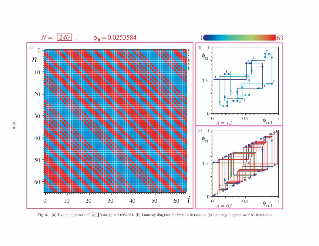
January12,
200614:18
01477
0 10 20 30 40 50 60
60
50
40
30
20
10
0
n
i
9876543210
N = 240 , φ = 0.02535840 0 63
n = 120 0.5 1
0
0.5
1
φ
φ
n-1
n
1
2
3
4
5
6
7
8
9
n = 630 0.5 1
0
0.5
1
φ
φ
n-1
n
Fig. 6. (a) Dynamic pattern of 240 from φ0 = 0.0253584. (b) Lameray diagram for first 12 iterations. (c) Lameray diagram over 63 iterations.
3791

January12,
200614:18
01477
0 10 20 30 40 50 60
60
50
40
30
20
10
0
n
i
N = 2 , φ = 0.643680 0 63
n = 60 0.5 1
0
0.5
1
φ
φ
n-1
n
n = 630 0.5 1
0
0.5
1
φ
φ
n-1
n
Fig. 7. (a) Dynamic pattern of 2 from φ0 = 0.64368. (b) Lameray diagram for first six iterations. (c) Lameray diagram over 63 iterations.
3792

January 12, 2006 14:18 01477
A Nonlinear Dynamics Perspective of Wolfram’s New Kind of Science. Part V 3793
N = 2 , φ = 0.3431840 0 250
n = 250 0.5 1
0
0.5
1
φ
φ
n-1
n
n = 300 0.5 1
0
0.5
1
φ
φ
n-1
n
n = 350 0.5 1
0
0.5
1
φ
φ
n-1
n
n = 500 0.5 1
0
0.5
1
φ
φ
n-1
n
n = 750 0.5 1
0
0.5
1
φ
φ
n-1
n
n = 1000 0.5 1
0
0.5
1
φ
φ
n-1
n
n = 1500 0.5 1
0
0.5
1
φ
φ
n-1
n
n = 2000 0.5 1
0
0.5
1
φ
φ
n-1
n
n = 2500 0.5 1
0
0.5
1
φ
φ
n-1
n
Fig. 8. Nine snapshots of the Lameray diagram of 2 starting from φ0 = 0.343184.
ten iterations of the Lameray diagram constructedfrom the characteristic function χ1
46are shown in
Fig. 11(b) and the continued iterations up to n = 63are shown in Fig. 11(c).
A comparison of the loci in Fig. 11(c) with theforward time-1 map of 46 in Table 2 (p. 1075)of [Chua et al., 2005] shows that except for theinitial point (which did not fall on the attractor but
belongs to its basin of attraction), all other pointsof the loci fall on the time-1 map of 46 .
To demonstrate this result holds for any otherinitial point belonging to the same basin of attrac-tion, Fig. 12 shows the Lameray diagram of 46(starting from a different initial point φ0 =0.888034) over n = 7, 15, 25, 50, 75, 100, 150, 200and 250 iterations, respectively. Again, except for

January12,
200614:18
01477
0 10 20 30 40 50 60
60
50
40
30
20
10
0
n
i
N = 3 , φ = 0.643680 0 63
n = 100 0.5 1
0
0.5
1
φ
φ
n-1
n
n = 630 0.5 1
0
0.5
1
φ
φ
n-1
n
Fig. 9. (a) Dynamic pattern of 3 from φ0 = 0.64368. (b) Lameray diagram for first ten iterations. (c) Lameray diagram over 63 iterations.
3794

January 12, 2006 14:18 01477
A Nonlinear Dynamics Perspective of Wolfram’s New Kind of Science. Part V 3795
N = 3 , φ = 0.5564120 0 250
n = 50 0.5 1
0
0.5
1
φ
φ
n-1
n
n = 100 0.5 1
0
0.5
1
φ
φ
n-1
n
n = 150 0.5 1
0
0.5
1
φ
φ
n-1
n
n = 200 0.5 1
0
0.5
1
φ
φ
n-1
n
n = 350 0.5 1
0
0.5
1
φ
φ
n-1
n
n = 500 0.5 1
0
0.5
1
φ
φ
n-1
n
n = 1000 0.5 1
0
0.5
1
φ
φ
n-1
n
n = 1500 0.5 1
0
0.5
1
φ
φ
n-1
n
n = 2500 0.5 1
0
0.5
1
φ
φ
n-1
n
Fig. 10. Nine snapshots of the Lameray diagram of 3 starting from φ0 = 0.556412.
the initial point, the loci of the Lameray diagram isseen to converge on the forward time-1 map of 46in Table 2 of [Chua et al., 2005].
2.6. Lameray diagram of 110
The dynamic pattern of the first 65 iterations ofrule 110 (with complexity index κ = 2) starting
from φ0 = 0.40653 is shown in Fig. 13(a). The firstfive iterations of the Lameray diagram constructedfrom the characteristic function χ1
110are shown in
Fig. 13(b) and the continued iterations up to n = 63are shown in Fig. 13(c).
A comparison of the loci in Fig. 13(c) with theforward time-1 map of 110 in Table 2 (p. 1091) of[Chua et al., 2005] shows that except for some initial

January12,
200614:18
01477
0 10 20 30 40 50 60
60
50
40
30
20
10
0
n
i
N = 46 , φ = 0.8953140 0 63
n = 100 0.5 1
0
0.5
1
φ
φ
n-1
n
n = 630 0.5 1
0
0.5
1
φ
φ
n-1
n
Fig. 11. (a) Dynamic pattern of 46 from φ0 = 0.895314. (b) Lameray diagram for first ten iterations. (c) Lameray diagram over 63 iterations.
3796
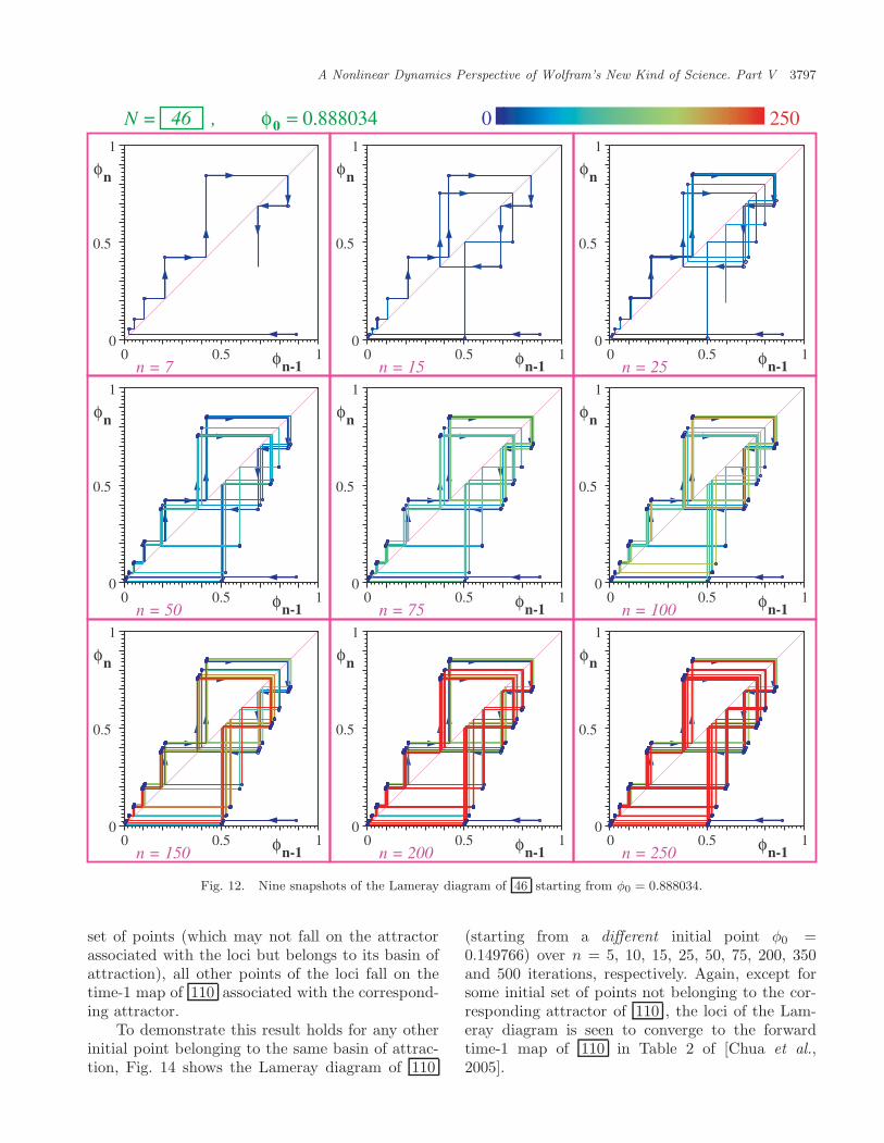
January 12, 2006 14:18 01477
A Nonlinear Dynamics Perspective of Wolfram’s New Kind of Science. Part V 3797
N = 46 , φ = 0.8880340 0 250
n = 70 0.5 1
0
0.5
1
φ
φ
n-1
n
n = 150 0.5 1
0
0.5
1
φ
φ
n-1
n
n = 250 0.5 1
0
0.5
1
φ
φ
n-1
n
n = 500 0.5 1
0
0.5
1
φ
φ
n-1
n
n = 750 0.5 1
0
0.5
1
φ
φ
n-1
n
n = 1000 0.5 1
0
0.5
1
φ
φ
n-1
n
n = 1500 0.5 1
0
0.5
1
φ
φ
n-1
n
n = 2000 0.5 1
0
0.5
1
φ
φ
n-1
n
n = 2500 0.5 1
0
0.5
1
φ
φ
n-1
n
Fig. 12. Nine snapshots of the Lameray diagram of 46 starting from φ0 = 0.888034.
set of points (which may not fall on the attractorassociated with the loci but belongs to its basin ofattraction), all other points of the loci fall on thetime-1 map of 110 associated with the correspond-ing attractor.
To demonstrate this result holds for any otherinitial point belonging to the same basin of attrac-tion, Fig. 14 shows the Lameray diagram of 110
(starting from a different initial point φ0 =0.149766) over n = 5, 10, 15, 25, 50, 75, 200, 350and 500 iterations, respectively. Again, except forsome initial set of points not belonging to the cor-responding attractor of 110 , the loci of the Lam-eray diagram is seen to converge to the forwardtime-1 map of 110 in Table 2 of [Chua et al.,2005].

January12,
200614:18
01477
0 10 20 30 40 50 60
60
50
40
30
20
10
0
n
i
N = 110 , φ = 0.406530 0 63
n = 50 0.5 1
0
0.5
1
φ
φ
n-1
n
n = 630 0.5 1
0
0.5
1
φ
φ
n-1
n
Fig. 13. (a) Dynamic pattern of 110 from φ0 = 0.40653. (b) Lameray diagram for first five iterations. (c) Lameray diagram over 63 iterations.
3798

January 12, 2006 14:18 01477
A Nonlinear Dynamics Perspective of Wolfram’s New Kind of Science. Part V 3799
N = 110 , φ = 0.1497660 0 500
n = 50 0.5 1
0
0.5
1
φ
φ
n-1
n
n = 100 0.5 1
0
0.5
1
φ
φ
n-1
n
n = 150 0.5 1
0
0.5
1
φ
φ
n-1
n
n = 250 0.5 1
0
0.5
1
φ
φ
n-1
n
n = 500 0.5 1
0
0.5
1
φ
φ
n-1
n
n = 750 0.5 1
0
0.5
1
φ
φ
n-1
n
n = 2000 0.5 1
0
0.5
1
φ
φ
n-1
n
n = 3500 0.5 1
0
0.5
1
φ
φ
n-1
n
n = 5000 0.5 1
0
0.5
1
φ
φ
n-1
n
Fig. 14. Nine snapshots of the Lameray diagram of 110 starting from φ0 = 0.149766.
2.7. Lameray diagram of 30
The dynamic pattern of the first 65 iterations ofrule 30 (with complexity index κ = 2) startingfrom φ0 = 0.895314 is shown in Fig. 15(a). Thefirst ten iterations of the Lameray diagram con-structed from the characteristic function χ1
30are
shown in Fig. 15(b), and the continued iterationsup to n = 63 are shown in Fig. 15(c).
A comparison of the loci in Fig. 15(c) with theforward time-1 map of 30 in Table 2 (p. 1071) of[Chua et al., 2005] shows that except for some ini-tial set of points (which do not fall on the attractorassociated with the loci but belong to its basin of
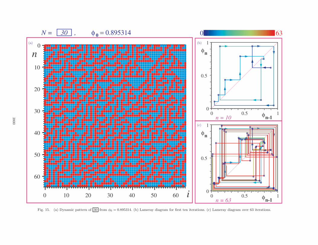
January12,
200614:18
01477
0 10 20 30 40 50 60
60
50
40
30
20
10
0
n
i
N = 30 , φ = 0.8953140 0 63
n = 100 0.5 1
0
0.5
1
φ
φ
n-1
n
n = 630 0.5 1
0
0.5
1
φ
φ
n-1
n
Fig. 15. (a) Dynamic pattern of 30 from φ0 = 0.895314. (b) Lameray diagram for first ten iterations. (c) Lameray diagram over 63 iterations.
3800

January 12, 2006 14:18 01477
A Nonlinear Dynamics Perspective of Wolfram’s New Kind of Science. Part V 3801
attraction), all other points of the loci fall on thetime-1 map of 30 associated with the correspond-ing attractor.
To demonstrate this result holds for any otherinitial point belonging to the same basin of attrac-tion, Fig. 16 shows the Lameray diagram of 30(starting from a different initial point φ0 =
0.149766) over n = 7, 14, 21, 50, 75, 100, 200,300 and 500 iterations, respectively. Again exceptfor some initial set of points not belonging to thecorresponding attractor of 30 , the loci of theLameray diagram is seen to converge to the for-ward time-1 map of 30 in Table 2 of [Chuaet al., 2005].
N = 30 , φ = 0.1497660 0 500
n = 70 0.5 1
0
0.5
1
φ
φ
n-1
n
n = 140 0.5 1
0
0.5
1
φ
φ
n-1
n
n = 210 0.5 1
0
0.5
1
φ
φ
n-1
n
n = 500 0.5 1
0
0.5
1
φ
φ
n-1
n
n = 750 0.5 1
0
0.5
1
φ
φ
n-1
n
n = 1000 0.5 1
0
0.5
1
φ
φ
n-1
n
n = 2000 0.5 1
0
0.5
1
φ
φ
n-1
n
n = 3000 0.5 1
0
0.5
1
φ
φ
n-1
n
n = 5000 0.5 1
0
0.5
1
φ
φ
n-1
n
Fig. 16. Nine snapshots of the Lameray diagram of 30 starting from φ0 = 0.149766.

January 12, 2006 14:18 01477
3802 L. O. Chua et al.
3. Characteristic Functions areFractals
A careful examination of the characteristic func-tions χ1
Nin Table 2 would reveal that each graph
of χ1N
is composed of many subpatterns which areself-similar in the sense that each can be rescaledby appropriate horizontal and vertical scaling fac-tors so that it coincides with a part of the compos-ite pattern. Let us illustrate this fractal geometry[Barnsley, 1988] with some examples.
Example 3.1 [Characteristic function χ12]. Let us
repeat the characteristic function χ12
from Table 2in Fig. 17(a) by passing a curve through the smallred and blue squares while deleting the red andblue vertical bars to avoid clutter. We will hence-forth refer to this curve as the graph of χ1
N.
Let us examine two subpatterns of this graph.Subpattern 1 covers the “cyan” rectangular areabounded by φ 2 ∈ [0.5, 1.0] and χ1
2∈ [0, 0.2]. To
show that this subpattern can be used as a tem-plate, which upon rescaling by appropriate hori-zontal and vertical scaling factors, can reproduceexactly corresponding portions of the graph atarbitrarily small scales, we have enlarged it assubpattern 1© in Fig. 17(a), by a factor of 2 in bothhorizontal and vertical directions.
Let us observe next that the smaller “cyan”rectangle “2” bounded by φ 2 ∈ [0.25, 0.5] and χ1
2∈
[0.5, 0.6] can be enlarged by a horizontal scale = 22
and a vertical scale = 22 to obtain the subpattern2© which is identical to the “template” 1© directlyabove it.
Let us examine next the smaller cyan rect-angle “3” in subpattern 2© bounded by φ 2 ∈[0.28125, 0.3125] and χ1
2∈ [0.5625, 0.575], and
observe that it too coincides with the template 1©upon enlarging it horizontally by 25 and verticallyby 25.
The above process can be repeated any numberof times with appropriate choice of scaling factors,commensurate with the computer word length.
Repeating the above scaling process to thethree small cyan rectangles labeled “4”, “5”, and“6” in Fig. 17(b), we obtain the three subpatternsshown in 4©, 5©, and 6© of Fig. 17(b), each one isagain found to be identical to the original template1© in Fig. 17(a).
We conclude therefore that the graph of χ12
near the origin consists of infinitely many scaledinfinitesimal subpatterns of template 1©. In other
words, the graph of χ12
exhibits a fractal geometryin the sense that it is composed of infinitely manyself-similar subpatterns.
Example 3.2 [Characteristic function χ13]. The
graph of characteristic function χ13
replotted fromTable 2 is shown in Fig. 18. By rescaling the threecyan rectangles labeled “1”, “2”, and “3” by appro-priate scaling factors, we obtain the correspondingsubpatterns 1©, 2© and 3© in Fig. 18. Observe thatthese three subpatterns are all identical. Continuingthis process, we found the graph of χ1
3is composed
of infinitely many scaled copies of template 1©.
Example 3.3 [Characteristic function χ110
]. Thegraph of characteristic function χ1
10replotted from
Table 2 is shown in Fig. 19. Observe the three cyanareas labeled “1”, “2”, and “3” are identical afterappropriate rescaling, as shown in subpatterns 1©,2© and 3© in Fig. 19.
Example 3.4 [Characteristic function χ111
]. Thegraph of characteristic function χ1
11is replotted
from Table 2 in Fig. 20. Observe the cyan arealabeled “1” and rescaled as template 1© containsinfinitely many scaled copies of itself, as illustratedin subpattern 2© in Fig. 20.
Example 3.5 [Characteristic function χ117
]. Thegraph of characteristic function χ1
17replot-
ted from Table 2 is shown in Fig. 21. Thefractal geometry of χ1
17is obvious from the rescaled
patterns 1© and 2©.
Example 3.6 [Characteristic function χ1110
]. Thegraph of characteristic function χ1
110replotted from
Table 2 is shown in Fig. 22. The two subpatterns 1©and 2© reveal the fractal geometry of χ1
110.
Example 3.7 [Characteristic function χ1124
]. Thegraph of characteristic function χ1
124replotted from
Table 2 is shown in Fig. 23. The two subpatterns 1©and 2© illustrate the fractal geometry of χ1
124.
Example 3.8 [Characteristic function χ1137
]. Thegraph of characteristic function χ1
137replotted from
Table 2 is shown in Fig. 24. The two subpatterns 1©and 2© reveal the fractal geometry of χ1
137.
Example 3.9 [Characteristic function χ1193
]. Thegraph of characteristic function χ1
193replotted from
Table 2 is shown in Fig. 25. The two subpatterns 1©and 2© reveal the fractal geometry of χ1
193.

January 12, 2006 14:18 01477
A Nonlinear Dynamics Perspective of Wolfram’s New Kind of Science. Part V 3803
0 0.1 0.2 0.3 0.4 0.5 0.6 0.7 0.8 0.9 10
0.1
0.2
0.3
0.4
0.5
0.6
0.7
0.8
0.9
1
φ
χ1
2
2
0.5 0.6 0.7 0.8 0.9 10
0.1
0.2
φ
χ1
2
2
0.25 0.3 0.35 0.4 0.45 0.50.5
0.55
0.6
φ
χ1
2
2
0.28125 0.2875 0.29375 0.3 0.30625 0.31250.5625
0.56875
0.575
φ
χ1
2
2
1
1
2
23
3
(a) subpattern 1©: horizontal scaling = 21,vertical scaling = 21
subpattern 2©: horizontal scaling = 22,vertical scaling = 22
subpattern 3©: horizontal scaling = 25,vertical scaling = 25
0 0.1 0.2 0.3 0.4 0.5 0.6 0.7 0.8 0.9 10
0.1
0.2
0.3
0.4
0.5
0.6
0.7
0.8
0.9
1
φ
χ1
2
2
0.125 0.15 0.175 0.2 0.225 0.250.25
0.275
0.3
φ
χ1
2
2
0.0625 0.075 0.0875 0.1 0.1125 0.1250.125
0.1375
0.15
φ
χ1
2
2
0.03125 0.0375 0.04375 0.05 0.05625 0.06250.0625
0.06875
0.075
φ
χ1
2
2
4
4
5
5
6
6
(b) subpattern 4©: horizontal scaling = 23,vertical scaling = 23
subpattern 5©: horizontal scaling = 24,vertical scaling = 24
subpattern 6©: horizontal scaling = 25,vertical scaling = 25
Fig. 17. Fractal compositions of χ12.

January 12, 2006 14:18 01477
3804 L. O. Chua et al.
0 0.1 0.2 0.3 0.4 0.5 0.6 0.7 0.8 0.9 10
0.1
0.2
0.3
0.4
0.5
0.6
0.7
0.8
0.9
1
φ
χ1
3
3
0.375 0.4 0.425 0.45 0.475 0.50.5
0.525
0.55
φ
χ1
3
3
0.1875 0.2 0.2125 0.225 0.2375 0.250.75
0.7625
0.775
φ
χ1
3
3
0.09735 0.1 0.10625 0.1125 0.11875 0.1250.875
0.88125
0.8875
φ
χ1
3
3
1
1
2
2
3
3
Fig. 18. Fractal compositions of χ13.
subpattern 1©: horizontal scaling = 23,vertical scaling = 23
subpattern 2©: horizontal scaling = 24,vertical scaling = 24
subpattern 3©: horizontal scaling = 25,vertical scaling = 25
0 0.1 0.2 0.3 0.4 0.5 0.6 0.7 0.8 0.9 10
0.1
0.2
0.3
0.4
0.5
0.6
0.7
0.8
0.9
1
φ
χ1
10
10
0.1885 0.2 0.2125 0.225 0.2375 0.250.375
0.3875
0.4
φ
χ1
10
10
0.09375 0.1 0.10625 0.1125 0.11875 0.1250.1875
0.19375
0.2
φ
χ1
10
10
0.04685 0.05 0.05311 0.05524 0.05937 0.06250.09375
0.09688
0.01
φ
χ1
10
10
1
1
2
2
3
3
Fig. 19. Fractal compositions of χ110
.
subpattern 1©: horizontal scaling = 24,vertical scaling = 24
subpattern 2©: horizontal scaling = 25,vertical scaling = 25
subpattern 3©: horizontal scaling = 26,vertical scaling = 26

January 12, 2006 14:18 01477
A Nonlinear Dynamics Perspective of Wolfram’s New Kind of Science. Part V 3805
0 0.1 0.2 0.3 0.4 0.5 0.6 0.7 0.8 0.9 10
0.1
0.2
0.3
0.4
0.5
0.6
0.7
0.8
0.9
1
φ
χ1
11
11
0.625 0.6375 0.65 0.6625 0.675 0.68750
0.01
0.02
0.03
0.04
0.05
0.06
φ
χ1
11
11
0.66409 0.66488 0.66566 0.66644 0.66722 0.6680
0.001
0.002
0.003
φ
χ1
11
11
1
1
2
2
Fig. 20. Fractal compositions of χ111
.
subpattern 1©: horizontal scaling = 24,vertical scaling = 24
subpattern 2©: horizontal scaling = 28,vertical scaling = 28
0 0.1 0.2 0.3 0.4 0.5 0.6 0.7 0.8 0.9 10
0.1
0.2
0.3
0.4
0.5
0.6
0.7
0.8
0.9
1
φ
χ1
17
17
0.6875 0.7 0.7125 0.725 0.7375 0.750
0.01
0.02
0.03
0.04
0.05
0.06
φ
χ1
17
17
0.731 0.732 0.733 0.7340
0.001
0.002
0.003
φ
χ1
17
17
1
1
2
2
Fig. 21. Fractal compositions of χ117
.
subpattern 1©: horizontal scaling = 24,vertical scaling = 24
subpattern 2©: horizontal scaling = 28,vertical scaling = 28
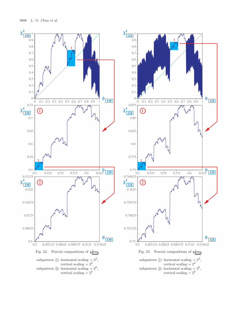
January 12, 2006 14:18 01477
3806 L. O. Chua et al.
0 0.1 0.2 0.3 0.4 0.5 0.6 0.7 0.8 0.9 10
0.1
0.2
0.3
0.4
0.5
0.6
0.7
0.8
0.9
1
φ
χ1
110
110
0.5 0.525 0.55 0.575 0.6 0.6250.5
0.55
0.6
0.65
0.7
0.75
φ
χ1
110
110
0.5 0.503125 0.50625 0.509375 0.5125 0.5156250.5
0.50625
0.5125
0.51875
0.525
0.53125
φ
χ1
110
110
1
1
2
2
Fig. 22. Fractal compositions of χ1110
.
subpattern 1©: horizontal scaling = 23,vertical scaling = 22
subpattern 2©: horizontal scaling = 26,vertical scaling = 25
0 0.1 0.2 0.3 0.4 0.5 0.6 0.7 0.8 0.9 10
0.1
0.2
0.3
0.4
0.5
0.6
0.7
0.8
0.9
1
φ
χ1
124
124
0.5 0.525 0.55 0.575 0.6 0.6250.75
0.775
0.8
0.825
0.85
0.875
φ
χ1
124
124
0.5 0.503125 0.50625 0.509375 0.5125 0.5156250.75
0.753125
0.75625
0.759375
0.7625
0.765625
φ
χ1
124
124
1
1
2
2
Fig. 23. Fractal compositions of χ1124
.
subpattern 1©: horizontal scaling = 23,vertical scaling = 23
subpattern 2©: horizontal scaling = 26,vertical scaling = 26

January 12, 2006 14:18 01477
A Nonlinear Dynamics Perspective of Wolfram’s New Kind of Science. Part V 3807
0 0.1 0.2 0.3 0.4 0.5 0.6 0.7 0.8 0.9 10
0.1
0.2
0.3
0.4
0.5
0.6
0.7
0.8
0.9
1
φ
χ1
137
137
0.9375 0.95 0.9625 0.975 0.9875 10.875
0.9
0.925
0.95
0.975
1
φ
χ1
137
137
0.996094 0.998047 10.992188
0.99375
0.995313
0.996875
0.998438
1
φ
χ1
137
137
1
1 2
2
Fig. 24. Fractal compositions of χ1137
.
subpattern 1©: horizontal scaling = 24,vertical scaling = 23
subpattern 2©: horizontal scaling = 28,vertical scaling = 27
0 0.1 0.2 0.3 0.4 0.5 0.6 0.7 0.8 0.9 10
0.1
0.2
0.3
0.4
0.5
0.6
0.7
0.8
0.9
1
φ
χ1
193
193
0.4375 0.45 0.4625 0.475 0.4875 0.50.1875
0.2
0.2125
0.225
0.2375
0.25
φ
χ1
193
193
0.464844 0.466797 0.468750.199218
0.199999
0.200781
0.201562
0.202343
0.203124
φ
χ1
193
193
1
1
2
2
Fig. 25. Fractal compositions of χ1193
.
subpattern 1©: horizontal scaling = 24,vertical scaling = 24
subpattern 2©: horizontal scaling = 28,vertical scaling = 28
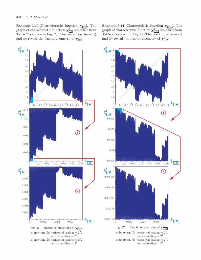
January 12, 2006 14:18 01477
3808 L. O. Chua et al.
Example 3.10 [Characteristic function χ130
]. Thegraph of characteristic function χ1
30replotted from
Table 2 is shown in Fig. 26. The two subpatterns 1©and 2© reveal the fractal geometry of χ1
30.
0 0.1 0.2 0.3 0.4 0.5 0.6 0.7 0.8 0.9 10
0.1
0.2
0.3
0.4
0.5
0.6
0.7
0.8
0.9
1
φ
χ1
30
30
0 0.01 0.02 0.03 0.04 0.05 0.060
0.02
0.04
0.06
0.08
0.1
0.12
φ
χ1
30
30
0 0.001 0.002 0.0030
0.001
0.002
0.003
0.004
0.005
0.006
φ
χ1
30
30
1
1
2
2
Fig. 26. Fractal compositions of χ130
.
subpattern 1©: horizontal scaling = 24,vertical scaling = 23
subpattern 2©: horizontal scaling = 28,vertical scaling = 27
Example 3.11 [Characteristic function χ1135
]. Thegraph of characteristic function χ1
135replotted from
Table 2 is shown in Fig. 27. The two subpatterns 1©and 2© reveal the fractal geometry of χ1
135.
0 0.1 0.2 0.3 0.4 0.5 0.6 0.7 0.8 0.9 10
0.1
0.2
0.3
0.4
0.5
0.6
0.7
0.8
0.9
1
φ
χ1
135
135
0 0.01 0.02 0.03 0.04 0.05 0.060.9375
0.95
0.9625
0.975
0.9875
1
φ
χ1
135
135
0 0.002 0.004 0.0060.992188
0.99375
0.995313
0.996875
0.998438
1
φ
χ1
135
135
1
12
2
Fig. 27. Fractal compositions of χ1135
.
subpattern 1©: horizontal scaling = 24,vertical scaling = 24
subpattern 2©: horizontal scaling = 27,vertical scaling = 27

January 12, 2006 14:18 01477
A Nonlinear Dynamics Perspective of Wolfram’s New Kind of Science. Part V 3809
Example 3.12 [Characteristic function χ190
]. Thegraph of characteristic function χ1
90replotted from
Table 2 is shown in Fig. 28. The two subpatterns 1©and 2© reveal the fractal geometry of χ1
90.
0 0.1 0.2 0.3 0.4 0.5 0.6 0.7 0.8 0.9 10
0.1
0.2
0.3
0.4
0.5
0.6
0.7
0.8
0.9
1
φ
χ1
90
90
0 0.01 0.02 0.03 0.04 0.05 0.060
0.02
0.04
0.06
0.08
0.1
0.12
φ
χ1
90
90
0 0.001 0.002 0.0030
0.001
0.002
0.003
0.004
0.005
0.006
φ
χ1
90
90
1
1
2
2
Fig. 28. Fractal compositions of χ190
.
subpattern 1©: horizontal scaling = 24,vertical scaling = 23
subpattern 2©: horizontal scaling = 28,vertical scaling = 27
Example 3.13 [Characteristic function χ1150
]. Thegraph of characteristic function χ1
150replotted from
Table 2 is shown in Fig. 29. The two subpatterns 1©and 2© reveal the fractal geometry of χ1
150.
0 0.1 0.2 0.3 0.4 0.5 0.6 0.7 0.8 0.9 10
0.1
0.2
0.3
0.4
0.5
0.6
0.7
0.8
0.9
1
φ
χ1
150
150
0 0.001 0.002 0.0030
0.001
0.002
0.003
0.004
0.005
0.006
φ
χ1
150
150
0 0.0001 0.00020
0.0001
0.0002
0.0003
0.0004
φ
χ1
150
150
1
1
2
2
Fig. 29. Fractal compositions of χ1150
.
subpattern 1©: horizontal scaling = 28,vertical scaling = 27
subpattern 2©: horizontal scaling = 212,vertical scaling = 211

January 12, 2006 14:18 01477
3810 L. O. Chua et al.
4. Predicting the Fractal Structures
The fractal structure of each characteristic func-tion χ1
Nin Table 2 can be analyzed and predicted
using the properties of characteristic functions tobe presented below, and from the coefficient b1 inthe explicit formulas from Table 1.
4.1. Two-level fractal stratifications
Let us partition the unit interval [0,1] into foursubintervals Φ1
∆= [0, 0.25), Φ2∆= [0.25, 0.5), Φ3
∆=[0.5, 0.75), and Φ4
∆= [0.75, 1.0]. It follows from thebinary-to-decimal conversion formula
{x0, x1, x2, . . . , xI} �→ φ =I∑
i=0
2−(i+1)xi (15)
that each binary string belonging to these foursubintervals must have the following form:
{0, 0, x2, x3, x4, . . . , xI} ∈ Φ1
{0, 1, x2, x3, x4, . . . , xI} ∈ Φ2
{1, 0, x2, x3, x4, . . . , xI} ∈ Φ3
{1, 1, x2, x3, x4, . . . , xI} ∈ Φ4
(16)
Let {y0, y1, y2, . . . , yI} denote the image of{x0, x1, x2, . . . , xI} under local rule N :
{x0, x1, x2, . . . , xI}T N�−→{y0, y1, y2, . . . , yI} (17)
where
{y0, y1, y2, . . . , yI} �→ χ1N (φ) (18)
and φ is the decimal representation in Eq. (15),namely,
χ1N
(φ) =I∑
i=0
2−(i+1)yi (19)
Observe that if we let the binary string{x0, x1, x2, . . . , xI} assume all binary combinationsfrom {0, 0, 0, . . . , 0} to {1, 1, 1, . . . , 1} in Eq. (17),and calculate the corresponding decimal valuefrom Eq. (19), we would obtain the coordinates(φN , χ1
N) for plotting the characteristic functions
in Table 2.Observe also that the first binary bit “y0” of
Eq. (17) is given by the first step function (i =0) in Table 1, as defined by Eq. (7). The valueof y0 is therefore determined by the three binary
bits
(x−1, x0, x1) = (xI , x0, x1) (20)
in view of the periodic boundary condition x−1 = xI
in Fig. 1(a). In other words, we have:
Property 4.1. The first binary bit y0 of χ1N
ofEq. (18) depends in general on the last binary bitxI of the input binary string of Eq. (15).
Since the first binary bit y0 of Eq. (18) con-tributes the largest component 2−1 = 0.5 (ify0 = 1), and since the last binary bit xI alter-nates between “0” and “1” as we increase φN fromφN = 0 to φN = 1 in Table 2, it follows that,depending on the formula in Table 1 for local ruleN , the characteristic function χ1
Nmay exhibit a
discontinuous jump in χ1N
equal to ∆χ1N
= 0.5.This implies that certain subintervals of χ1
Nmay
exhibit vertical jumps equal to 0.5 between adjacentred and blue bars in Table 2, resulting in a two-levelstratification of χ1
N.
In view of Property 4.1, the characteristic func-tion χ1
Nin Table 2 may exhibit a discontinuous
jump by an amount equal to ∆χ1N
= 0.5 overdifferent subintervals Φ1, Φ2, Φ3 and Φ4, respec-tively. An examination of the graph of each charac-teristic function χ1
Nin Table 2 shows that within
each subinterval Φi, one of the following groupingsof small red squares (resp. blue squares) on topof each thin red bar (resp. blue bar) apply to allsmall squares located within the same subintervalΦi, i = 1, 2, 3, 4 (this information is coded in colorred, blue or violet, in Table 5):
Group 1. All small red squares have χ1N
≥ 0.5and all small blue squares (in the case where thereare two-level stratifications) have χ1
N< 0.5. In this
case, we will paint the upper rectangle of N incolumn Φi of Table 5 in red, and the rectangle belowit will be painted blue.
Group 2. The small red and blue squares arelocated opposite to those of Group 1. In this case,the upper rectangle of Table 5 will be painted blue,and the lower rectangle will be painted red.
Group 3. There is no stratification and all smalladjacent red and blue squares have χ1
N≥ 0.5. In
this case, only the upper rectangle is painted in vio-let color,2 while the lower rectangle is left blank.
2We have chosen the violet color as the nearest approximation of the color combination between the red and blue colors.

January 12, 2006 14:18 01477
A Nonlinear Dynamics Perspective of Wolfram’s New Kind of Science. Part V 3811
Table 5. Stratification of characteristic functions over subintervals Φ1 ∈ [0, 0.25), Φ2 ∈ [0.25, 0.5), Φ3 ∈ [0.5, 0.75), andΦ4 ∈ [0.75, 1].
30
Φ4Φ3Φ2Φ1N
0
1
2
3
4
5
31
29
28
27
26
25
24
23
22
21
20
19
18
17
16
15
14
13
12
11
10
9
8
7
6
62
Φ4Φ3Φ2Φ1N
32
33
34
35
36
37
63
61
60
59
58
57
56
55
54
53
52
51
50
49
48
47
46
45
44
43
42
41
40
39
38

January 12, 2006 14:18 01477
3812 L. O. Chua et al.
Table 5. (Continued )
94
Φ4Φ3Φ2Φ1N
64
65
66
67
68
69
95
93
92
91
90
89
88
87
86
85
84
83
82
81
80
79
78
77
76
75
74
73
72
71
70
126
Φ4Φ3Φ2Φ1N
96
97
98
99
100
101
127
125
124
123
122
121
120
119
118
117
116
115
114
113
112
111
110
109
108
107
106
105
104
103
102

January 12, 2006 14:18 01477
A Nonlinear Dynamics Perspective of Wolfram’s New Kind of Science. Part V 3813
Table 5. (Continued )
158
Φ4Φ3Φ2Φ1N
128
129
130
131
132
133
159
157
156
155
154
153
152
151
150
149
148
147
146
145
144
143
142
141
140
139
138
137
136
135
134
190
Φ4Φ3Φ2Φ1N
160
161
162
163
164
165
191
189
188
187
186
185
184
183
182
181
180
179
178
177
176
175
174
173
172
171
170
169
168
167
166

January 12, 2006 14:18 01477
3814 L. O. Chua et al.
Table 5. (Continued )
222
Φ4Φ3Φ2Φ1N
192
193
194
195
196
197
223
221
220
219
218
217
216
215
214
213
212
211
210
209
208
207
206
205
204
203
202
201
200
199
198
254
Φ4Φ3Φ2Φ1N
224
225
226
227
228
229
255
253
252
251
250
249
248
247
246
245
244
243
242
241
240
239
238
237
236
235
234
233
232
231
230

January 12, 2006 14:18 01477
A Nonlinear Dynamics Perspective of Wolfram’s New Kind of Science. Part V 3815
Group 4. The small red and blue squares arelocated opposite to those of Group 3. In this case,only the lower rectangle is painted in violet color,while the upper rectangle is left blank.
4.1.1. Stratification prediction procedure
The color painted in each of the two rectangleslocated in each subinterval Φi of the characteristicfunction χ1
Nof Table 5 is obtained by inspection
of the graph of χ1N
in Table 2. We will now showhow these colors can be predicted directly from the“firing patterns” [Chua et al., 2003] of each ruleN ; namely, from the “three-bit pattern” associ-ated with each red vertex of the Boolean cube rep-resenting N in Fig. 1(e).
Our goal is to determine the color of thefirst output bit y0 from these firing patterns. Inparticular, y0 depends on the three binary bits{x−1, x0 and, x1}, as shown in Fig. 30, where x−1
= xI in view of the periodic boundary conditionin Fig. 1(a). The “color” of x0 and x1 in Fig. 30is chosen from the subinterval Φi as defined by thefirst two columns of Eq. (16); namely,
Φi x0 x1
Φ1 0 0Φ2 0 1Φ3 1 0Φ4 1 1
The color of x−1 in Fig. 30 is chosen as follows:
1. x−1 = 0, if xI = 0
Using the bar-coloring scheme described inp. 1049 of [Chua et al., 2005], this corresponds to
1x− 0x 1x
0y
NT
Fig. 30. The left-most output bit y0 of χ1N
is “1” if
{x−1, x0, x1} = {xI , x0, x1} is a firing pattern of N .Otherwise, y0 = 0.
the case where the right-most bar of χ1N
in Table 2is a red bar.
2. x−1 = 1, if xI = 1
This corresponds to the case where the right-most bar of χ1
Nin Table 2 is a blue bar.
Since both x−1 and y0 can assume a “0” or a“1”, there are four possible outcomes:
Outcome 1 : x−1 = 0 , y0 = 0
In this case, all bars belonging to subinterval Φi arecolored red and lie below χ1
N= 0.5.
Outcome 2 : x−1 = 0 , y0 = 1
In this case, all bars belonging to subinterval Φi arecolored red and lie above χ1
N= 0.5.
Outcome 3 : x−1 = 1 , y0 = 0
In this case, all bars belonging to subinterval Φi arecolored blue and lie below χ1
N= 0.5.
Outcome 4 : x−1 = 1 , y0 = 1
In this case, all bars belonging to subinterval Φi arecolored blue and lie above χ1
N= 0.5.
4.1.2. Examples illustrating stratificationprediction procedure
Let us illustrate the above “stratification predic-tion” procedure with some examples.
Example 4.1 [Predicting Stratification for χ116
].The Boolean cube for rule 16 is reproduced fromTable 1 of [Chua et al., 2003] in Fig. 31(a). Sinceonly vertex 4© is painted red in this Boolean cube,there is only one firing pattern → 1 00 , as shown in Fig. 31(b).
For each subinterval Φi, i = 1, 2, 3, 4, we insertthe corresponding x0 and x1 as specified in thepreceding table. We then assign x−1 = 0 (for redbars) on the left column and x−1 = 1 (for blue bars)on the right column for each Φi. The color of y0 ineach case is then determined from the firing pat-terns in Fig. 31(b). In this case, y0 = 1 only in (row1, column 2). Since y0 = 0 in the left column of Φ1
and y0 = 1 in the right column of Φ1, it follows thatχ1
16has two stratifications over the subinterval Φ1,
where the red bars are below χ116
= 0.5 and the bluebars are above χ1
16= 0.5.

January 12, 2006 14:18 01477
3816 L. O. Chua et al.
16T
Firing Pattern
Φ4
Φ3
Φ2
Φ1
1x− 0x 1x
0 0 0
00y
1x− 0x 1x
0 0 1
00y
1x− 0x 1x
0 1 0
0y
1x− 0x 1x
0 1 1
00y
1x− 0x 1x
1 0 0
10y
1x− 0x 1x
1 0 1
00y
1x− 0x 1x
1 1 0
0y
1x− 0x 1x
1 1 1
00y
162 3
1
5
0
4
6 7
0 0
16T
16T
16T
16T
16T
16T
16T
16T
Fig. 31. Predicting stratification for rule 16 . (a) Boolean cube for 16 . (b) Firing patterns for 16 . (c) Stratificationdetermination data.

January 12, 2006 14:18 01477
A Nonlinear Dynamics Perspective of Wolfram’s New Kind of Science. Part V 3817
Since y0 = 0 for all other cases in Fig. 31(c),it follows that there are no stratifications insubinterval Φ2, Φ3 and Φ4, and all red and bluebars in these three subintervals are located belowχ1
16= 0.5, as is indeed the case in Table 2.
Example 4.2 [Predicting Stratification for χ12].
The Boolean cube for rule 2 is shown in Fig. 32(a).It has only one firing pattern → 00 1 , as shown in Fig. 32(b). The correspond-ing stratification determination data is shown inFig. 32(c). From these data, we conclude thatonly subinterval Φ2 has a stratification in χ1
2
where all red bars lie above, and all blue barslie below χ1
2= 0.5. Since y0 = 0 in the other
three subintervals Φ1, Φ3 and Φ4, all red andblue bars must lie below χ1
2= 0.5. Observe
that this prediction is consistent with Table 2, asexpected.
Example 4.3 [Predicting Stratification for χ14].
The Boolean cube for rule 4 is shown in Fig. 33(a).It has only one firing pattern → 0 1 0 ,as shown in Fig. 33(b). In this case, only subinter-val Φ3 in Fig. 33(c) has a stratification in χ1
4where
all red bars must lie above χ14
= 0.5, and all bluebars must lie below χ1
4= 0.5. All red and blue bars
in the other three subintervals Φ1, Φ2 and Φ4 must
lie below χ14
= 0.5, because y0 = 0. Again, thisprediction is consistent with Table 2.
Example 4.4 [Predicting Stratification for χ1110
].The Boolean cube for rule 110 is shown inFig. 34(a). It has five firing patterns, →0 0 1 , → 0 1 0 , →0 1 1 , → 1 0 1 , → 11 0 , as shown in Fig. 34(b). The stratificationdetermination data in Fig. 34(c) shows only subin-terval Φ4 has a stratification where all red bars mustlie above χ1
110= 0.5, and all blue bars must lie
below it.Since y0 = 0 in both columns of Φ1, it follows
that all red and blue bars must lie below χ1110
= 0.5.On the other hand, since y0 = 1 in both
columns of Φ2 and Φ3, it follows that all red andblue bars in subintervals Φ2 and Φ3 must lie aboveχ1
110= 0.5. All of these predictions are consistent
with Table 2, as expected.
4.1.3. {Φ1,Φ2,Φ3,Φ4} — stratified families
If we examine the color of the rectangles of the foursubintervals Φ1, Φ2, Φ3 and Φ4 in Table 5 and codeeach violet rectangle by a “0” binary bit, and allother rectangles by a “1” binary bit, we will dis-cover the first 16 rules follow the four-bit binarynumber system as shown below, henceforth calledthe stratified family “0”.
N ψ 1Φ 2Φ 3Φ 4Φ EquivalentDecimal Number
0 0ψ 0 0 0 0 0
1
2
3
4
5
6
7
8
9
10
11ψ 1 0 0
22ψ 0 1 0
33ψ 1 1 0
44ψ 0 0 1
55ψ 1 0 1
66ψ 0 1 1
77ψ 1 1 1
88ψ 0 0 0 1
99ψ 1 0 0 1
1010ψ 0 1 0 1
1111ψ 1 1 0 1 11
1212ψ 0 0 1 1 12
1313ψ 1 0 1 1 13
1414ψ 0 1 1 1 14
Stratified
Family
“0”
1515ψ 1 1 1 1 15
0
0
0
0
0
0
0
Observe that the color background of Table 1 is determined from this coding scheme, where “0” iscoded “light blue”, while “1” is coded “light pink” in Table 1.

January 12, 2006 14:18 01477
3818 L. O. Chua et al.
2T
Firing Pattern
Φ4
Φ3
Φ2
Φ1
1x− 0x 1x
0 0 0
00y
1x− 0x 1x
0 0 1
10y
1x− 0x 1x
0 1 0
0y
1x− 0x 1x
0 1 1
00y
1x− 0x 1x
1 0 0
00y
1x− 0x 1x
1 0 1
00y
1x− 0x 1x
1 1 0
0y
1x− 0x 1x
1 1 1
00y
0 0
2T
2T
2T
2T
2T
2T
2T
2T
22 3
1
5
0
4
6 7
Fig. 32. Predicting stratification for rule 2 . (a) Boolean cube for 2 . (b) Firing patterns for 2 . (c) Stratificationdetermination data .

January 12, 2006 14:18 01477
A Nonlinear Dynamics Perspective of Wolfram’s New Kind of Science. Part V 3819
4T
Firing Pattern
Φ4
Φ3
Φ2
Φ1
1x− 0x 1x
0 0 0
00y
1x− 0x 1x
0 0 1
00y
1x− 0x 1x
0 1 0
0y
1x− 0x 1x
0 1 1
00y
1x− 0x 1x
1 0 0
00y
1x− 0x 1x
1 0 1
00y
1x− 0x 1x
1 1 0
0y
1x− 0x 1x
1 1 1
00y
1 0
4T
4T
4T
4T
4T
4T
4T
4T
42 3
1
5
0
4
6 7
Fig. 33. Predicting stratification for rule 4 . (a) Boolean cube for 4 . (b) Firing patterns for 4 . (c) Stratificationdetermination data .

January 12, 2006 14:18 01477
3820 L. O. Chua et al.
2 3
1
5
0
4
6 7
110
Φ4
Φ3
Φ2
Φ1
1x− 0x 1x
0 0 0110
T
00y
1x− 0x 1x
0 0 1110
T
10y
1x− 0x 1x
0 1 0110
T
10y
1x− 0x 1x
0 1 1110
T
10y
1x− 0x 1x
1 0 0110
T
00y
1x− 0x 1x
1 0 1110
T
10y
1x− 0x 1x
1 1 0110
T
10y
1x− 0x 1x
1 1 1110
T
00y
110T
110T
110T
110T
Firing Patterns
110T
Fig. 34. Predicting stratification for rule 110 . (a) Boolean cube for 110 . (b) Firing patterns for 110 . (c) Stratificationdetermination data .

January 12, 2006 14:18 01477
A Nonlinear Dynamics Perspective of Wolfram’s New Kind of Science. Part V 3821
Observe that no two members of the stratifiedfamily “0” have identical four-bit binary patterns.Since there are only 16 distinct combinations of fourbinary bits, the stratified family “0” had alreadyconsumed all of them and it is clear that the remain-ing rules in Table 5 must consist of repetitions
of these patterns. A careful analysis of the next16 rules reveals, however, that the four-bit binarypatterns of the next 16 rules {16, 17, . . . , 31} aremere permutations of the stratified family “0”,as illustrated below (henceforth called stratifiedfamily “1”):
N ψ 1Φ 2Φ 3Φ 4Φ EquivalentDecimal Number
16 0ψ 1 0 0
171ψ 0 0 0
182ψ 1 1 0
193ψ 0 1 0
204ψ 1 0 1
215ψ 0 0 1
226ψ 1 1 1
237ψ 0 1 1
248ψ 1 0 0
259ψ 0 0 0
2610ψ 1 1 0
2711ψ 0 1 0
2812ψ 1 0 1
2913ψ 0 0 1
3014ψ 1 1 1
Stratified
Family
“1”
3115ψ 0 1 1
0
0
0
0
0
0
0
0
1
1
1
1
1
1
1
1
1
0
3
2
5
4
7
6
9
8
11
10
13
12
15
14
Observe that the 4-bit code ψ = {Φ1,Φ2,Φ3,Φ4} of stratified family “1” and stratified family “0” arerelated by a 16 × 16 permutation matrix; namely,
ψ0(1)ψ1(1)ψ2(1)ψ3(1)ψ4(1)ψ5(1)ψ6(1)ψ7(1)ψ8(1)ψ9(1)ψ10(1)ψ11(1)ψ12(1)ψ13(1)ψ14(1)ψ15(1)
=
0 0 0 0 0 0 0 0 0 0 0 0 0 0 00 0 0 0 0 0 0 0 0 0 0 0 0 0 0
0 0 0 0 0 0 0 0 0 0 0 0 0 0 00 0 0 0 0 0 0 0 0 0 0 0 0 0 00 0 0 0 0 0 0 0 0 0 0 0 0 0 00 0 0 0 0 0 0 0 0 0 0 0 0 0 00 0 0 0 0 0 0 0 0 0 0 0 0 0 00 0 0 0 0 0 0 0 0 0 0 0 0 0 00 0 0 0 0 0 0 0 0 0 0 0 0 0 00 0 0 0 0 0 0 0 0 0 0 0 0 0 00 0 0 0 0 0 0 0 0 0 0 0 0 0 00 0 0 0 0 0 0 0 0 0 0 0 0 0 00 0 0 0 0 0 0 0 0 0 0 0 0 0 00 0 0 0 0 0 0 0 0 0 0 0 0 0 00 0 0 0 0 0 0 0 0 0 0 0 0 0 00 0 0 0 0 0 0 0 0 0 0 0 0 0 0
︸ ︷︷ ︸M1,0
ψ0(0)ψ1(0)ψ2(0)ψ3(0)ψ4(0)ψ5(0)ψ6(0)ψ7(0)ψ8(0)ψ9(0)ψ10(0)ψ11(0)ψ12(0)ψ13(0)ψ14(0)ψ15(0)

January 12, 2006 14:18 01477
3822 L. O. Chua et al.
It turns out that the remaining rules can bepartitioned in a similar way into a stratified family“2”, “3”, . . . ,“15”. Together, these 16 families corre-spond exactly to the 16 rules listed in the 16 pages ofTable 1, respectively. Let us summarize this remark-able organization as follows:
Property 4.2. The 16 rules listed in each of the16 pages of Table 1 form a stratified family whosefour-bit binary patterns ψ(k), k = 0, 1, 2, . . . , 15, arerelated to each other by a 16×16 permutation matrix
ψ(k) = Mk,l ψ(l)
Table 6 lists 16 matrices which transform ψ(0) fromstratified family “0” into ψ(k) of stratified family“k”, k = 0, 1, 2, . . . , 15.
The four-bit binary patterns of the last eightrules of each stratified family “k” can be obtainedby copying the four-bit binary patterns of the firsteight rules and then complementing the fourth bitcorresponding to Φ4. Observe that, in Table 5, thefour color codes of all Φi’s of each local rule N isequivalent to the vertically-switched color codes ofall Φi’s of the corresponding local rule 255 − N asillustrated below:
,
For example, the color code of each Φi of 0 ,24 , 120 and 220 in Table 5 can be obtainedby switching vertically the color code of the
corresponding Φi of 255 , 231 , 135 and 35 ,respectively.
4.2. Rules having no fractalstratifications
Since the occurrence of two-level stratificationscomes from the term b1x−1 [i = 0 in Eq. (7)] inTable 1, it follows that no such stratification canoccur in χ1
Nif b1 = 0 for rule N . An examina-
tion of Table 2 shows that there are only 16 ruleswith b1 = 0. These 16 xI -insensitive rules are listedin Table 7. Observe that these 16 rules can be gen-erated from the following formula:
N = 17β , β = 0, 1, 2, . . . , 15
This relationship can be derived from Table 6. Inparticular, since the right-most bit xI -insensitiverules corresponds to ψi = {Φ1,Φ2,Φ3,Φ4} ={0, 0, 0, 0}, it follows from Tables 1 and 6 thatψi = {0, 0, 0, 0} is repeated after integer multipliesof 17, and hence all xI -insensitive rules N mustsatisfy N = 17k, k = 0, 1, 2, . . . , 15.
These 16 rules are composed of the correspond-ing (k + 1)th members in the stratified family “k”,k = 0, 1, 2, . . . , 15. For example, 0 is the first mem-ber of the stratified family “0”, 17 is the secondmember of the stratified family “1”, . . . , and 225 isthe sixteenth member of the stratified family “15”.
Property 4.3. The following 16 characteristic func-tions have no stratifications:
Single-Level Fractalsχ1
0, χ1
17, χ1
34, χ1
51χ1
68, χ1
85, χ1
102, χ1
119,
χ1136
, χ1153
, χ1170
, χ1187
, χ1204
, χ1221
, χ1238
, and χ1255
4.3. Origin of the fractal structures
We will now uncover a basic mechanism responsi-ble for the presence of fractals in the characteris-tic functions shown in Table 2. Let us examine aninfinitesimally small neighborhood of the origin ofχ1
Nby considering the input string
0, 0, . . . , 0︸ ︷︷ ︸first k entries
, xk, xk+1, . . . , xI
�→ φ
=I∑
i=0
2−(i+1)xi (21)
If we multiply φ by 2k in Eq. (21), we would obtain
φ • 2k =I∑
i=k
2−(i+1)+kxi =I−k∑j=0
2−(j+1)xj (22)
where j � (i−k). Observe that, as I → ∞, Eq. (22)converges to the binary string in Eq. (15). It fol-lows that no matter how close the binary stringin Eq. (21) is to the origin, we can always rescaleit to recover the original string in Eq. (15). More-over, except possibly for the (k + 1)th term xk = 1,all other terms xk+1, xk+2, . . . , xI in Eq. (21) will

January 12, 2006 14:18 01477
A Nonlinear Dynamics Perspective of Wolfram’s New Kind of Science. Part V 3823
Table 6. List of 16 permutation matrices Mk,l which transform ψ(0) from stratified family “0” into ψ(k) of stratified family“k”, k = 0, 1, 2, . . . , 15.

January 12, 2006 14:18 01477
3824 L. O. Chua et al.
Table 6. (Continued )

January 12, 2006 14:18 01477
A Nonlinear Dynamics Perspective of Wolfram’s New Kind of Science. Part V 3825
Table 7. List of 16 right-most bit xI -insensitive local rules.
255238221204
187170153136
1191028568
5134170
generate the same corresponding output binary bityi, i = k + 1, k + 2, . . . , I, because the same localrule N is used. Hence, by rescaling χ1
Naccord-
ingly, we can recover the corresponding originalgraph. To determine the appropriate scaling factor,it is necessary to examine the output binary bit yi,i = 0, 1, 2, . . . , k − 1 because it may not be zero fortwo reasons:
(i) yk−1 = 1 if
(xk−2, xk−1, xk) = (0, 0, 1)T N�−→ 1 (23)
In other words, if is a firing pattern [Chuaet al., 2003] of Rule N , or equivalently, if vertex1© in the Boolean cube in Fig. 1(e) is painted in redcolor.
(ii) yi = 1 if
(xi−1, xi, xi+1) = (0, 0, 0)T N�−→ 1 (24)
for i = 0, 1, 2, . . . , k − 2. In other words, ifis a firing pattern of Rule N , or
equivalently, if vertex 0© in the Boolean cube inFig. 1(e) is painted in red color. Let us examinenow the consequences of the occurrence of one orboth of these two cases. There are four possiblescenarios:
Scenario 1. (0, 0, 0) is not a firing pattern3 but(0, 0, 1) is a firing pattern of N , and xI = 0.
An example satisfying scenario 1 is Rule 2 ,where vertex 0© is blue but vertex 1© is red. In thiscase, yk−1 = 1 and the output binary pattern has
the form0, 0, . . . , 0, yk−1︸ ︷︷ ︸
first k terms
, yk, yk+1, . . . , yI
�→ χ1
N
=I∑
i=k−1
2−(i+1)yi (25)
Multiplying the right side of Eq. (25) by 2(k−1) weobtain
χ1N (2k−1) =
I∑i=k−1
2−(i+1)+(k−1)yi
=I−k+1∑
j=0
2−(j+1)yj
=I∑
i=0
2−(i+1)yi, as I → ∞ (26)
Hence, by multiplying the output string in Eq. (25)by the factor 2(k−1), we obtain Eq. (26), which isidentical to Eq. (18) as I → ∞. In other words,in Scenario 1, the characteristic function χ1
Narbi-
trarily near the origin can be rescaled to obtain thecorresponding original graph by multiplying φN by2k and χ1
Nby 2(k−1).
Scenario 2. (0, 0, 0) is not a firing pattern but(1, 0, 0) is a firing pattern of N , and xI = 1 withb1 �= 0.
In this case, y0 = 1 in view of Eq. (19), and theoutput binary string assumes the form:
{1, 0, 0, . . . , 0, yk−1, yk, yk+1, . . . , yI}
�→ 12
+I∑
i=k−1
2−(i+1)yi (27)
It follows from Eq. (27) that
χ̃1N � χ1
N − 12
=I∑
i=k−1
2−(i+1)yi
=I∑
i=0
2−(i+1)yi, as I → ∞ (28)
as in Eq. (26). Hence, apart from a translation by∆χ1
N= 1/2, the infinitesimal pattern near the
origin can be rescaled to coincide with the corre-sponding original pattern.
3An examination of the Boolean cubes in Table 1 of [Chua et al., 2003] shows (0, 0, 0) is not a firing pattern for rules with aneven number: i.e. N = 2n, n = 0, 1, 2, . . . , 128.

January 12, 2006 14:18 01477
3826 L. O. Chua et al.
Scenario 3. (0, 0, 0) is a firing pattern of N , andxI = 0.
In this case, yi, i = 0, 1, 2, . . . , k − 2; namely, 1, 1, . . . , 1,︸ ︷︷ ︸
first k−1 terms
yk−1, yk, yk+1, . . . , yI
�→ χ1
N (29)
where
χ1N =
k−2∑i=0
2−(i+1) +I∑
i=k−1
2−(i+1)yi
= 1 − 2−(k−1) +I∑
i=k−1
2−(i+1)yi (30)
It follows from Eq. (30) that
χ̃1N � 1 − χ1
N = 2−(k−1) −I∑
i=k−1
2−(i+1)yi (31)
Multiplying both sides of Eq. (31) by the scalingfactor 2(k−1), we obtain
χ̃1N • 2(k−1) = 1 −
I∑i=k−1
2−(i+1)+(k−1)yi
= 1 −I∑
i=0
2−(i+1)yi, as I → ∞ (32)
as in Eq. (26).Since Eq. (32) is an affine transformation of
Eq. (26), it follows that the fractal pattern arbitrar-ily near the origin is preserved upon scaling, apartfrom an affine transformation.
Scenario 4. (0, 0, 0) is a firing pattern of N , but(1, 0, 0) is not a firing pattern of N , and xI = 1with b1 �= 0.
In this case, y0 = 0, in view of Eq. (18); namely,0, 1, 1, . . . , 1, yk−1︸ ︷︷ ︸
first k terms
, yk, yk+1, . . . , yI
�→ χ1
N (33)
where
χ1N =
I∑i=1
2−(i+1)yi
=k−2∑i=1
2−(i+1) +I∑
i=k−1
2−(i+1)yi
=12− 2−(k−1) +
I∑i=k−1
2−(i+1)yi (34)
It follows from Eq. (34) that
χ̃1N �
(1 − χ1
N
)− 1
2
= 2−(k−1) −I∑
i=k−1
2−(i+1)yi
= 2−(k−1) −I∑
i=0
2−(i+1)yi, as I → ∞ (35)
as in Eq. (26).Since Eq. (34) is an affine transformation of
Eq. (26), it follows that the fractal pattern arbitrar-ily near the origin is preserved upon scaling, apartfrom an affine transformation.
5. Gardens of Eden
A cursory inspection of the graphs of the character-istic functions χ1
Ndisplayed in Table 2 reveals that
most of these graphs exhibit a discontinuous jumpover a finite range ∆χ1
N= χ1
N(φ+
jump)−χ1N
(φ−jump)
at various discrete points φjump ∈ [0, 1] where allpoints within the interval (χ1
N(φ+
jump),χ1N
(φ−jump))
have no preimage under χ1N
. Such a characteristicfunction is therefore not a surjective (onto) func-tion. Points within such intervals are special casesof the following interesting class of initial bit-stringconfigurations.
Definition 5.1. Garden of Eden of N . An (I +1)-bit binary string {x0, x1, x2, . . . , xI} is saidto be a garden of Eden of a local rule N iff itdoes not have a predecessor under the local ruletransformation TN .
It follows from Definition 5.1 that a garden ofEden φ0 �
∑Ii=0 2−(i+1)xi of N can never occur as
a point on an orbit of N arising from some initialbit-string configuration whose decimal equivalent isdifferent from φ0. Hence, a garden of Eden has nopast, but only present and future.4
4The name garden of Eden was first introduced by Moore in the context of von Neumann’s self-reproducing automata [Moore,1962].

January 12, 2006 14:18 01477
A Nonlinear Dynamics Perspective of Wolfram’s New Kind of Science. Part V 3827
Table 8. A compendium of all gardens of Eden (colored in green) over the range [0, 1] of χ1N
.
χ =10
χ =11
χ =12
χ =13
χ =14
χ =15
χ =16
χ =17
χ =18
χ =19
χ =110
χ =111
χ =112
χ =113
χ =114
χ =115
χ =116
χ =117
χ =118
χ =119
χ =120
χ =121
χ =122
χ =123
χ =124
χ =125
χ =126
χ =127
χ =128
χ =129
χ =130
χ =131
χ =132
χ =133
χ =134
χ =135
χ =136
χ =137
χ =138
χ =139
χ =140
χ =141
χ =142
χ =143
χ =144
χ =145
χ =146
χ =147
χ =148
χ =149
χ =150
χ =151
χ =152
χ =153
χ =154
χ =155
χ =156
χ =157
χ =158
χ =159
χ =160
χ =161
χ =162
χ =163

January 12, 2006 14:18 01477
3828 L. O. Chua et al.
Table 8. (Continued )
χ =164
χ =165
χ =166
χ =167
χ =168
χ =169
χ =170
χ =171
χ =172
χ =173
χ =174
χ =175
χ =176
χ =177
χ =178
χ =179
χ =180
χ =181
χ =182
χ =183
χ =184
χ =185
χ =186
χ =187
χ =188
χ =189
χ =190
χ =191
χ =192
χ =193
χ =194
χ =195
χ =196
χ =197
χ =198
χ =199
χ =1100
χ =1101
χ =1102
χ =1103
χ =1104
χ =1105
χ =1106
χ =1107
χ =1108
χ =1109
χ =1110
χ =1111
χ =1112
χ =1113
χ =1114
χ =1115
χ =1116
χ =1117
χ =1118
χ =1119
χ =1120
χ =1121
χ =1122
χ =1123
χ =1124
χ =1125
χ =1126
χ =1127

January 12, 2006 14:18 01477
A Nonlinear Dynamics Perspective of Wolfram’s New Kind of Science. Part V 3829
Table 8. (Continued )
χ =1128
χ =1129
χ =1130
χ =1131
χ =1132
χ =1133
χ =1134
χ =1135
χ =1136
χ =1137
χ =1138
χ =1139
χ =1140
χ =1141
χ =1142
χ =1143
χ =1144
χ =1145
χ =1146
χ =1147
χ =1148
χ =1149
χ =1150
χ =1151
χ =1152
χ =1153
χ =1154
χ =1155
χ =1156
χ =1157
χ =1158
χ =1159
χ =1160
χ =1161
χ =1162
χ =1163
χ =1164
χ =1165
χ =1166
χ =1167
χ =1168
χ =1169
χ =1170
χ =1171
χ =1172
χ =1173
χ =1174
χ =1175
χ =1176
χ =1177
χ =1178
χ =1179
χ =1180
χ =1181
χ =1182
χ =1183
χ =1184
χ =1185
χ =1186
χ =1187
χ =1188
χ =1189
χ =1190
χ =1191

January 12, 2006 14:18 01477
3830 L. O. Chua et al.
Table 8. (Continued )
χ =1192
χ =1193
χ =1194
χ =1195
χ =1196
χ =1197
χ =1198
χ =1199
χ =1200
χ =1201
χ =1202
χ =1203
χ =1204
χ =1205
χ =1206
χ =1207
χ =1208
χ =1209
χ =1210
χ =1211
χ =1212
χ =1213
χ =1214
χ =1215
χ =1216
χ =1217
χ =1218
χ =1219
χ =1220
χ =1221
χ =1222
χ =1223
χ =1224
χ =1225
χ =1226
χ =1227
χ =1228
χ =1229
χ =1230
χ =1231
χ =1232
χ =1233
χ =1234
χ =1235
χ =1236
χ =1237
χ =1238
χ =1239
χ =1240
χ =1241
χ =1242
χ =1243
χ =1244
χ =1245
χ =1246
χ =1247
χ =1248
χ =1249
χ =1250
χ =1251
χ =1252
χ =1253
χ =1254
χ =1255

January 12, 2006 14:18 01477
A Nonlinear Dynamics Perspective of Wolfram’s New Kind of Science. Part V 3831
Table 9. A compendium of period-n isles of Eden of N .
Table 9-1(a). Period-1 isles of Eden.
* Here I +1 must be divisible by 3.
134 140 142 148 150 156 158
162 166 170 172 174 176 180
182 184 186 188 190 196 198
204 206 212 214 220 222 226
228 230 234 236 238 240 242
244 246 248 250 252 254
128 130 132 134 136 138 140
142 144 146 148 150 152 154
156 158 160 162 168 170 176
184 186 192 194 196 198 200
202 204 206 208 210 212 214
216 220 224 226 240 242
4 6 7 12 14 15 20
21 22 23 30 31 68 84
85 86 87 132 134 135 140
142 143 148 149 150 151 158
159 196 204 206 207 212 213
214 215 220 221 222 223
72 73 76 104 105 108 109
200 201 204 205 233 236 237
72 76 200 204 236
200 204 205 236 237
45 101 173 204 205 229
74 75 88 89 204
3
8*
7*
6
5
4
2
1
Rules Endowed with Isle of EdenPeriod-1 Isle of Edenn
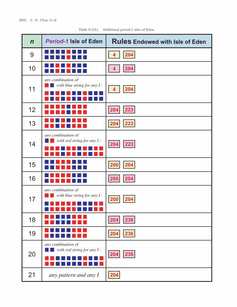
January 12, 2006 14:18 01477
3832 L. O. Chua et al.
Table 9-1(b). Additional period-1 isles of Eden.
any combination ofwith red string for any I :
any combination ofwith blue string for any I :
4 204
4 204
4 204
204 223
204 223
204 223
200 204
200 204
200 204
204 236
204 236
204 236
204
any combination ofwith blue string for any I :
any combination ofwith red string for any I :
9
10
11
12
13
14
15
16
17
18
19
any pattern and any I21
20
Rules Endowed with Isle of EdenPeriod-1 Isle of Edenn

January 12, 2006 14:18 01477
A Nonlinear Dynamics Perspective of Wolfram’s New Kind of Science. Part V 3833
Table 9-2. Period-2 isles of Eden.
3
any pattern and any I4
2
1
Rules Endowed with Isle of EdenPeriod-2 Isle of Edenn
13 15 27 29 35 41 43
49 51 57 59 69 71 77
79 85 93 97 99 105 107
113 115 121
32 33 34 35 40 41 42
43 48 49 51 59 96 97
104 105 106 107 112 113 115
120 121 123 168 169 170 171
187 224 225 232 233 234 235
240 241 243 248 249 251
18 19 22 23 50 51 54
55 146 147 150 151 178 179
182 182
51
For n = 1, Period-2 Isles of Eden can exist for any I.
For n = 2, Period-2 Isles of Eden can exist for any I + 1 that is divisible by 2.
For n = 3, Period-2 Isles of Eden can exist for any I + 1 that is divisible by 4.
Remarks :
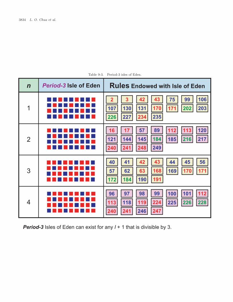
January 12, 2006 14:18 01477
3834 L. O. Chua et al.
Table 9-3. Period-3 isles of Eden.
3
4
2
1
Rules Endowed with Isle of EdenPeriod-3 Isle of Edenn
Period-3 Isles of Eden can exist for any I + 1 that is divisible by 3.
2 3 42 43 75 99 106
107 130 131 170 171 202 203
226 227 234 235
16 17 57 89 112 113 120
121 144 145 184 185 216 217
240 241 248 249
40 41 42 43 44 45 56
57 62 63 168 169 170 171
172 184 190 191
96 97 98 99 100 101 112
113 118 119 224 225 226 228
240 241 246 247

January 12, 2006 14:18 01477
A Nonlinear Dynamics Perspective of Wolfram’s New Kind of Science. Part V 3835
Table 9-4. Period-4 isles of Eden.
3
4
2
1
Rules Endowed with Isle of EdenPeriod-4 Isle of Edenn
Period-4 Isles of Eden can exist for any I + 1 that is divisible by 4.
10 15 170 175
80 85 240 245
15
85

January 12, 2006 14:18 01477
3836 L. O. Chua et al.
Table 9-5(a). Period-5 isles of Eden.
6
159
215
20
82 83 87 114 115 119
26 27 31 58 58 63
3 7 35 39 163 167
5
4
6
7
3
2
1
Rules Endowed with Isle of EdenPeriod-5 Isle of Edenn

January 12, 2006 14:18 01477
A Nonlinear Dynamics Perspective of Wolfram’s New Kind of Science. Part V 3837
Table 9-5(b). Additional period-5 isles of Eden.
113 121 185 240 241 249
43 107 170 171 227 235
96 97 98 112 113 240
17 21 49 53 117 181
40 41 42 43 56 170
15 43
85 113
12
11
13
14
10
9
8
Rules Endowed with Isle of EdenPeriod-5 Isle of Edenn
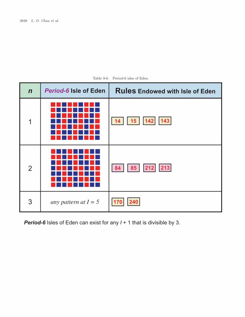
January 12, 2006 14:18 01477
3838 L. O. Chua et al.
Table 9-6. Period-6 isles of Eden.
any pattern at I = 53
2
1
Rules Endowed with Isle of EdenPeriod-6 Isle of Edenn
14 15 142 143
84 85 212 213
170 240
Period-6 Isles of Eden can exist for any I + 1 that is divisible by 3.
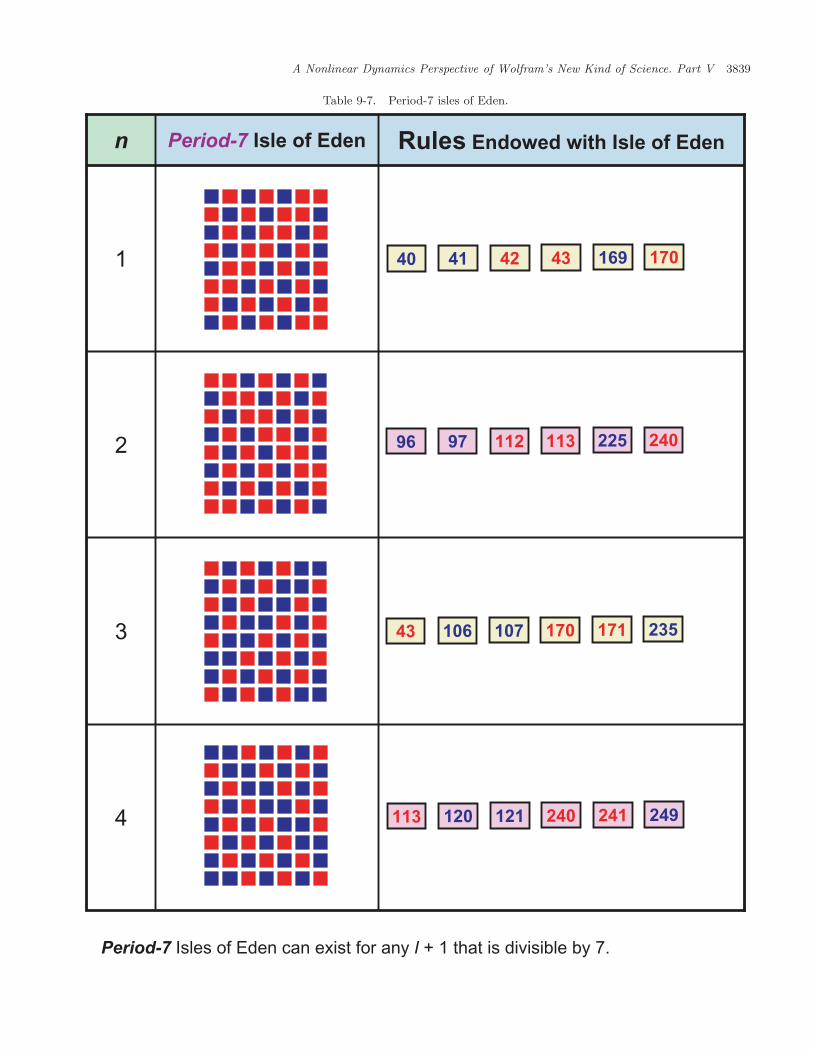
January 12, 2006 14:18 01477
A Nonlinear Dynamics Perspective of Wolfram’s New Kind of Science. Part V 3839
Table 9-7. Period-7 isles of Eden.
3
4
2
1
Rules Endowed with Isle of EdenPeriod-7 Isle of Edenn
Period-7 Isles of Eden can exist for any I + 1 that is divisible by 7.
40 41 42 43 169 170
96 97 112 113 225 240
43 106 107 170 171 235
113 120 121 240 241 249

January 12, 2006 14:18 01477
3840 L. O. Chua et al.
Table 9-8(a). Period-8 isles of Eden.
3
4
2
1
Rules Endowed with Isle of EdenPeriod-8 Isle of Edenn
40 41 42 43 56 169 170
96 97 98 112 113 225 240
43 106 107 170 171 227 235
113 120 121 185 240 241 249

January 12, 2006 14:18 01477
A Nonlinear Dynamics Perspective of Wolfram’s New Kind of Science. Part V 3841
Table 9-8(b). Additional period-8 isles of Eden.
Period-8 Isles of Eden can exist for any I + 1 that is divisible by 4.
14 15 142 143
84 85 212 2136
5
Rules Endowed with Isle of EdenPeriod-8 Isle of Edenn

January 12, 2006 14:18 01477
3842 L. O. Chua et al.
Table 9-9. Period-9 isles of Eden.
40 41 42 43 169 170
Period-9 Isles of Eden can exist for any I + 1 that is divisible by 9.
96 97 112 113 225 240
43 106 107 170 171 235
113 120 121 240 241 249
3
4
2
1
Rules Endowed with Isle of EdenPeriod-9 Isle of Edenn

January 12, 2006 14:18 01477
A Nonlinear Dynamics Perspective of Wolfram’s New Kind of Science. Part V 3843
Table 9-10(a). Period-10 isles of Eden.
40 41 42 43 169 170
96 97 112 113 225 240
43 106 107 170 171 2353
2
1
Rules Endowed with Isle of EdenPeriod-10 Isle of Edenn

January 12, 2006 14:18 01477
3844 L. O. Chua et al.
Table 9-10(b). Additional period-10 isles of Eden.
6
5
4
Rules Endowed with Isle of EdenPeriod-10 Isle of Edenn
113 120 121 240 241 249
Period-10 Isles of Eden can exist for any I + 1 that is divisible by 5.
14 15 142 143
84 85 212 213

January 12, 2006 14:18 01477
A Nonlinear Dynamics Perspective of Wolfram’s New Kind of Science. Part V 3845
Table 9-11(a). Period-11 isles of Eden.
40 41 42 43 169 170
96 97 112 113 225 240
43 106 107 170 171 235
3
2
1
Rules Endowed with Isle of EdenPeriod-11 Isle of Edenn

January 12, 2006 14:18 01477
3846 L. O. Chua et al.
Table 9-11(b). Additional period-11 isles of Eden.
113 120 121 240 241 249
40 41 42 43 169 170
96 97 112 113 225 240
6
5
4
Rules Endowed with Isle of EdenPeriod-11 Isle of Edenn

January 12, 2006 14:18 01477
A Nonlinear Dynamics Perspective of Wolfram’s New Kind of Science. Part V 3847
Table 9-11(c). Additional period-11 isles of Eden.
43 106 107 170 171 235
113 120 121 240 241 249
Period-11 Isles of Eden can exist for any I + 1 that is divisible by 11.
8
7
Rules Endowed with Isle of EdenPeriod-11 Isle of Edenn
Observe that any binary string
{x0, x1, x2, . . . , xI} �→ φ0 =I∑
i=0
2−(i+1)xi (36)
which has no preimage under χ1N
(i.e. φ0 does notbelong to the range of χ1
N) is a garden of Eden of
N . In other words, φ0 ∈ [0, 1] is a garden of Edenof N if there does not exist a φ−1 ∈ [0, 1] suchthat φ0 = χ1
N(φ−1), where φ−1 �= φ0. Note that
this property is only a sufficient condition for φ0
to be a garden of Eden. In the next section, we willsee that there exist some rather special points which
violate this property, but is nevertheless a garden ofEden because it satisfies Definition 5.1.
A compendium of all gardens of Eden belongingto each local rule N is listed in Table 8. Each pointφ0 ∈ [0, 1] printed in green along the χ1
Naxis does
not have a preimage under χ1N
and is therefore agarden of Eden.
6. Isle of Eden
For most rules N , there exist some specialperiod-1 points which have no predecessors in thesense that no orbits from other initial bit-string

January 12, 2006 14:18 01477
3848 L. O. Chua et al.
Table 10. Rules without period-k isles of Eden, k < 12.
255253239231219218211209
199197195193189165164161
157155153141139137133129
127126125124122117116111
1101031029594929190
8178706766656461
6052474638373628
25241198510
configurations can converge to such points, andhence they are also gardens of Eden in view ofDefinition 5.1. Moreover, since each of these pointsis a period-1 point, they have a preimage underχ1
N; namely, itself. Such special points (obtained
by exhaustive computer search) are henceforthcalled isles of Eden of N . Observe that an isle ofEden has no past, and no future (in the poetic sensethat time stood still)!
A compendium of all period-1 isles of Eden ofN for binary strings of various length I +1 is listedin Tables 9-1(a) and 9-1(b).
Let us now generalize the concept ofperiod-1 isle of Eden for “time-n” characteristicfunctions χn
N. Since such special period-n points
also have no predecessors under the “nth iterated”map χn
N, they are henceforth called period-n isles
of Eden. Table 9-k lists all period-k isles of Eden,k = 1, 2, 3, . . . , 11, obtained by an exhaustive com-puter search over all binary bit-strings of lengthI + 1 = 8, 9, 10, 11, respectively. In most cases, thesame bit-string configurations can be extended toarbitrarily large I, provided I + 1 is divisible bysome integer specified in the table.
Finally, we remark that based on exhaustivecomputer search, there are 64 local rules that donot have period-k isles of Eden, at least for k < 12.They are listed in Table 10.
7. Concluding Remarks
We have demonstrated that except for the eightaffine (mod 1 ) rules listed in Table 3, the graphof all characteristic functions χ1
Nin Table 2 are
endowed with a fractal structure. Indeed, eventhe graph of the eight affine (mod 1) rules canbe considered to exhibit a degenerate form of frac-tal structure since arbitrarily short segments of the
graph can be made to coincide with correspondingportions of the original graphs by appropriate affinetransformations. We have traced the origin of thesefractals to the decimal representation of binary bit-strings in Eq. (2), as well as to the local rule, whichmust apply to any bit string, regardless of the num-ber of “zeros” in front of it.
The explicit formulas in Table 1 for convert-ing any bit string {x0, x1, x2, . . . , xI} into a realnumber χ1
N∈ [0, 1] is remarkable for its scope of
potential applications. Indeed, these formulas canbe interpreted as a digital-to-analog converter inclosed form. Such formulas could not have beenderived without the explicit “universal” formuladerived in [Chua et al., 2003] for all local rules.
The widespread presence of period-k “isles ofEden” came as a surprise since they certainly haveno counter part in hyperbolic differential equations.To dramatize this phenomenon, we end Part V withour following poetic interpretation of the above newphenomenon: Hidden within the “garden of Eden”,which has no past, one finds immortality in an “isleof Eden”, which has neither past nor future.
Acknowledgments
This paper is supported in part by the MURIcontract no. N00014-03-1-0698, the DURINTcontract no. N00014-01-0741, the MARCO Micro-electronics Advances Research Corporation FENAAward no. 442521/WK57015, the NSF grant CHE-0103447, the UNIVERSITE du SUD, TOULON-VAR, France, the Foundations Francqui Fonds,Belgium, and the ministry of university researchand education, Italy, under the field project numberRBNE012NFW.
References
Barnsley, M. F. [1988] Fractals Everywhere (AcademicPress).
Billingsley, P. [1978] Ergodic Theory and Information(Robert Keirger Publishing Company, Huntington).
Chua, L. O., Yoon, S. & Dogaru, R. [2002] “A nonlineardynamics perspective of Wolfram’s new kind of sci-ence. Part I: Threshold of complexity,” Int. J. Bifur-cation and Chaos 12, 2655–2766.
Chua, L. O., Sbitnev, V. I. & Yoon, S. [2003] “A non-linear dynamics perspective of Wolfram’s new kind ofscience. Part II: Universal neuron,” Int. J. Bifurcationand Chaos 13, 2377–2491.
Chua, L. O., Sbitnev, V. I. & Yoon, S. [2004] “A non-linear dynamics perspective of Wolfram’s new kind of

January 12, 2006 14:18 01477
A Nonlinear Dynamics Perspective of Wolfram’s New Kind of Science. Part V 3849
science. Part III: Predicting the unpredictable,” Int.J. Bifurcation and Chaos 14, 3689–3820.
Chua, L. O., Sbitnev, V. I. & Yoon, S. [2005] “A non-linear dynamics perspective of Wolfram’s new kindof science. Part IV: From Bernoulli shift to 1/f spec-trum,” Int. J. Bifurcation and Chaos 15, 1045–1183.
Devaney, R. L. [1992] A First Course in ChaoticDynamic Systems: Theory and Experiment (Addison-Wesley, Reading, MA).
Moore, E. F. [1962] “Machine models of self-reproduction,” Proc. Fourteenth Symp. Applied Math-ematics, pp. 17–33.


