1192 M. BARBARY, PENG ZONG, A NOVEL STEALTHY TARGET DETECTION BASED ON STRATOSPHERIC …
A Novel Stealthy Target Detection Based on Stratospheric
Balloon-borne Positional Instability due to Random Wind
Mohamed A. BARBARY1, Peng ZONG
2
1 Dept. of Electronic and Information Engineering, Nanjing University of Aeronautics and Astronautics, Nanjing, China 2 Dept. of Astronautics, Nanjing University of Aeronautics and Astronautics, Nanjing, China
[email protected], [email protected]
Abstract. A novel detection for stealthy target model
F-117A with a higher aspect vision is introduced by using
stratospheric balloon -borne bistatic system. The potential
problem of the proposed scheme is platform instability
impacted on the balloon by external wind force. The flight
control system is studied in detail under typical random
process, which is defined by Dryden turbulence spectrum.
To accurately detect the stealthy target model, a real Radar
Cross Section (RCS) based on physical optics (PO) formu-
lation is applied. The sensitivity of the proposed scheme
has been improved due to increasing PO-scattering field of
stealthy model with higher aspect angle comparing to the
conventional ground-based system. Simulations demon-
strate that the proposed scheme gives much higher location
accuracy and reduces location errors.
Keywords
Stealthy RCS, bistatic balloon-borne radar, PO
method.
Introduction 1.
The complexity of stealth target detection is not only
related to the target itself, but also influenced by the elec-
tromagnetic environment [1]. The countering-stealth tech-
nologies are increasingly relevant, and research in this field
is ongoing around the world. Stealth technology mostly
focuses on defeating conventional ground-based detection
radar. Thus, the success of counter stealth endeavors is
focused mostly on novel and unique air defense infrastruc-
ture configurations. The Radar Cross Section (RCS) is
an important evaluation criterion of aircraft’s stealthy
performance, the envelope of the backscatter from stealthy
target varies rapidly with aspect angle. The shaping of
stealthy objects to reduce the backscattered energy towards
the radar is believed to be less effective when bistatic radar
is used [2].
Several researches deal with improving stealthy target
detection and tracking based on ground-based bistatic or
netted radar system [2–8]. Theses researches didn’t evalu-
ate bistatic radar sensitivity and performance of stealthy
target with a higher aspect vision. Since the bistatic radar
system might be mounted on higher altitude platforms to
achieve a larger probability of detecting stealthy target, the
bistatic radar sensitivity will be improved due to increasing
the scattered field of stealthy target with higher altitude. In
this paper, we investigate a novel technique for stealthy
target detection based on balloon–borne bistatic radar
system. The stations are positioned in the stratosphere
about 21 km above the Earth and kept stable in a sphere of
radius of 0.5 km [9]. To achieve high location accuracy for
stealthy target, the proposed scheme uses a physical optics
method (PO) to predict the real RCS of stealthy target. This
will better represent the actual situation of the stealthy
target detection.
One of the open research issues is whether the plat-
forms positional instability due to sudden gusts of strato-
spheric winds. In the aerospace field, the study of turbu-
lence effects is of fundamental importance in a lot of
different aspects [10], such as improvements of the aerody-
namic and structural analysis, prediction of expected be-
havior of a balloon-borne platform under various levels of
turbulence, evaluation of the stability of onboard sensing
equipment, and so on. Subject to the extreme complexity of
the turbulence phenomena and due to the huge variety of
applications, there is not a unique full-comprehensive
model for the atmospheric turbulence, but there exist
a wide variety of different and simplified models [11–12].
Numerous turbulence models are enumerated and de-
scribed. The most commonly adopted model to study the
impact of the turbulent wind gust on the balloon-borne is
the Dryden model. According to this model, the atmo-
spheric turbulence is modeled as a random velocity process
added by balloon-borne velocity vector described in
a body-fixed Cartesian coordinate system.
The rest of this paper is organized as follows. In Sec-
tion 2, we present balloon positional instability analysis
and random wind mathematical model. In Section 3, we
discuss the PO formulation to predict RCS of stealth
model. The bistatic range-measurement accuracy adopted
for unstable position of the proposed scheme using stealth
RCS is discussed in Section 4. Performance of the pro-
posed scheme is evaluated via computer simulation in
Section 5, followed by the conclusion in Section 6.

RADIOENGINEERING, VOL. 23, NO. 4, DECEMBER 2014 1193
Balloon Positional Instability 2.
Analysis
The general dynamic equations of a stratospheric
balloon platform are derived for flight over flat and non-
rotating Earth, considering buoyancy, added mass and
relevant conceptual design data of the stratospheric plat-
form. To include the effect of jet stream as a moving wind
field, the dynamic equations of motion can be derived in
the relative wind-axes, inertial wind-axes, or body-axes
coordinate systems [13–14]. The relative wind-axes system
is more convenient than other coordinate systems because
it expresses the wind-effect terms explicitly, bringing easier
understanding. Fig. 1 illustrates the relationship between
horizontal wind vector, airspeed velocity vector, and local
(Earth-fixed) velocity of the platform. The wind-relative
velocity vector is defined by airspeed 𝑉, flight path angle
𝛾, and heading 𝜓.
From Fig. 1, the inertial flight velocity with respect to
the local ENU frame is determined as:
𝑉𝐼 = �̇�𝑖 𝑢 + �̇�𝑖 𝑒 + �̇�𝑖 𝑛
= 𝑉 +𝑊
= 𝑉 sin 𝛾 𝑢 + (𝑉 cos 𝛾 sin𝜓 +𝑊𝐸)𝑒 + (𝑉 cos 𝛾 cos𝜓 +𝑊𝑁)𝑛
= 𝑉𝐼 sin 𝛾𝐼 𝑢 + 𝑉𝐼 cos 𝛾𝐼 sin𝜓𝐼 𝑒 + 𝑉𝐼 cos 𝛾𝐼 cos𝜓𝐼 𝑛 . (1)
Fig. 1. Balloon –borne velocity in the local and wind-relative
frames.
2.1 The Random Wind Mathematical Model
The Dryden model is one of the most useful and trac-
table models for atmospheric turbulence [13]. To define it
we need a body-fixed reference frame attached to the grav-
ity center of balloon-borne which moves with the target.
The x-axis is on the position of motion direction, y-axis is
on position along the wings, and z-axis is perpendicular to
the balloon-borne plane. Then, the turbulence is modeled
by adding some random components to balloon-borne
velocity defined in the body-fixed coordinate system.
An important consideration in this paper is the effect of
steady-state horizontal winds. The horizontal wind velocity
vector is defined as:
𝑊𝐻 = 𝑊 sin𝜓𝑤𝑒 + 𝑊 cos𝜓𝑤𝑛 , (2)
= 𝑊𝐸 𝑒 + 𝑊𝑁 𝑛 . (3)
In Dryden model continuous-time random processes
are modeled as zero-mean, Gaussian-distributed processes
whose PSD have analytic form given by [10–12]:
𝑆𝑒(𝜔) = 𝜎𝑒2𝐿𝑒𝜋𝑉0
1
1 + (𝐿𝑒𝑉0𝜔)
2 , (4)
𝑆𝑛(𝜔) = 𝜎𝑛2𝐿𝑛2𝜋𝑉0
1 + 3 (𝐿𝑛𝑉0𝜔)
2
[1 + (𝐿𝑛𝑉0𝜔)
2
]2 (5)
where 𝑉0 is the gust wind speed in the balloon-borne sys-
tem. The parameters 𝜎𝑒2 and 𝜎𝑛
2 depend on the level of
turbulence to be simulated and are selected accordingly
[11]. Parameters 𝐿𝑒 and 𝐿𝑛 are the scale lengths for the
PSDs and depend on the flight altitude. The mean wind
velocity at the altitude of 21 km varies between -15 to
+15 m/s [9]. Fig. 2 shows the PSDs of (4) and (5) for 𝜎𝑒 =
𝜎𝑛 = 𝜎𝑤 =15 m/s, 𝐿𝑒 = 𝐿𝑛 =533.54 m, and 𝑉0 = 15 m/s. To
reflect higher level of turbulence, the curves would be
multiplied by the desired values of 𝜎𝑒2 and 𝜎𝑛
2.
Fig. 2. PSD of Dryden velocity processes.
From (4) and (5), simulation model of wind can be
written as:
�̇�𝐸 +𝑉0𝐿𝑒𝑊𝐸 = √
2𝑉0𝐿𝑒𝜉𝑒 , (6a)
�̇�1 +𝑉0𝐿𝑛𝑊1 = (√3 − 1)√
𝑉0𝐿𝑛𝜉𝑛, (6b)
�̇�𝑁 +𝑉0𝐿𝑛𝑊1 +
𝑉0𝐿𝑛𝑊𝑁 = √
3𝑉0𝐿𝑛𝜉𝑛 (6c)
where 𝑊1 is the transition variable for calculating the wind
field model, 𝜉𝑒 and 𝜉𝑛 are the random variables subject to
normal distribution 𝑁 (0, 𝜎𝑤2).
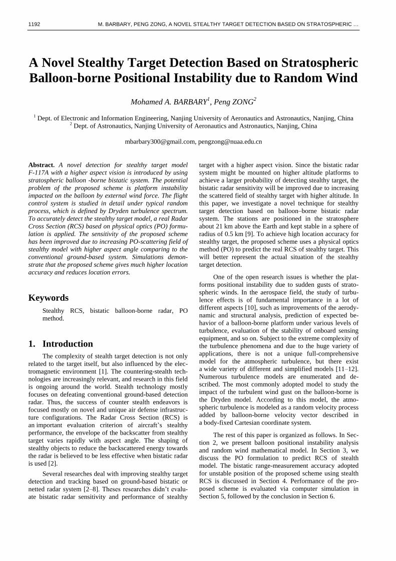
2.2 External Forces Acting on Balloon Plat-
form
The external forces acting on balloon-borne platform
include aerodynamic lift L and drag D, thrust T, weight W
and buoyancy B. We also consider a generic lateral force N,
which may be generated by any means, such as rolling the
lift vector through a small angle, 𝜙, or applying lateral
thrust. A free-body diagram of the forces in x-z plane is
shown in Fig. 3.
0 0.5 1 1.5 2 2.5 30
0.2
0.4
0.6
0.8
1
1.2
1.4
1.6
1.8
W (Rad/s)
Po
we
r sp
ectr
al d
en
sity (
m2 /s)
PSD of W
N
PSD of WE
1194 M. BARBARY, PENG ZONG, A NOVEL STEALTHY TARGET DETECTION BASED ON STRATOSPHERIC …
Fig. 3. External forces acting on balloon- borne platform.
The equations of motion are described by equating the
time derivative of the momentum vector with the sum of
external forces.
∑𝐹 =𝑑
𝑑𝑡(𝑀 𝑉𝐼)
= [(𝐵 −𝑊) sin 𝛾 + 𝑇 cos(𝛼 + 𝜇) − 𝐷 ]�̂�
+𝑁�̂� + [(𝑊 − 𝐵) cos 𝛾 − 𝐿 − 𝑇 sin(𝛼 + 𝜇) ]�̂� (7)
where L and D are the lift and drag forces, respectively.
The lift and drag coefficients from Lee [15] are used, and
are assumed to vary only with angle of attack. 𝜇 represents
the tilting angle of the propellers installed on both sides of
the airship. The lift and drag force can be calculated by
𝐿 = 𝑞. 𝑉𝑂𝐿2 /3. 𝐶𝐿(𝛼) , 𝐷 = 𝑞. 𝑉𝑂𝐿2 3⁄ . 𝐶𝐷(𝛼) , (8a)
𝐶𝐿(𝛼) = 0.590𝛼4 + 1.2231𝛼3 + 0.3248𝛼2 + 0.921𝛼
+ 0.0118,
𝐶𝐷(𝛼) = 0.340 𝛼4 + 0.0662𝛼3 + 1.2248𝛼2 + 0.0334𝛼
+0.04 (8b)
where q and VOL represent the dynamic pressure of free stream
and envelope volume of the platform.
The required thrust and power are given by [15]
𝑇 = 𝑞. 𝑉𝑂𝐿2 3⁄ . 𝐶𝐷, 𝑃 = 𝑇. 𝑉.1
𝜂𝑝𝜂𝑚 (9)
where 𝜂𝑝 and 𝜂𝑚 represent the efficiency of the propellers
and electric motor equipped in the airship. The values 0.7
and 0.9 are used for the efficiencies, respectively
The buoyancy force is another typical discriminator
between LTA vehicles and conventional aircraft. It plays
the role of lifting balloons upward and is equal to the
weight of displaced air by its volume immersed in the at-
mosphere. The net lift that can be available for payload,
system, and structure is determined by subtracting the
weight of the lift gas and envelope [15]:
𝐿𝑛𝑒𝑡 = 𝐵 −𝑊 = 𝑉𝑂𝐿 (𝜌𝑎−𝜌ℎ)𝑔 −𝑊𝑒𝑛𝑣 , 𝐵 = 𝑉𝑂𝐿. 𝜌𝑎 . 𝑔 (10)
where 𝜌𝑎 and 𝜌ℎ refer to the density of the surrounding
atmosphere and helium, respectively. For the helium that is
generally used as the lifting gas, the gross lift per unit
volume (𝜌𝑎−𝜌ℎ)𝑔 is 10.359 N/m3.
By Newton’s second law, the force equilibrium
equation in the inertial frame is expressed as
𝐹 = 𝑚𝑇𝑎 = 𝑚𝑇 (𝑑𝑉𝐼𝑑𝑡)𝐼 ,
𝑚𝑇 = 𝑚 +𝑚𝑎𝑥 +𝑚𝑎𝑦 +𝑚𝑎𝑧 (11)
where 𝑚𝑇 includes the empty mass m and the added
masses, 𝑚𝑎𝑥, 𝑚𝑎𝑦, and 𝑚𝑎𝑧. When a body moves through
fluid, it must push some mass of fluid out on the way. If the
body is accelerated, the surrounding fluid must also be
accelerated. Under this circumstance, the body behaves as
if it were heavier, so that mass is added. The diagonal
terms of added mass tensor are the main terms on the body
axes of balloon for 𝑚𝑎𝑥, 𝑚𝑎𝑦, and 𝑚𝑎𝑧 of (11) respectively.
Because it is assumed that air density varies in a unit at
operating altitude, the values should be multiplied by cor-
responding density to obtain added mass in the optimiza-
tion process:
𝑀𝑎 =
[2.1391 × 10⁴ 1.6502 × 10⁻¹² 1.3365 × 10⁻¹¹
−2.0890 × 10⁻¹² 2.4363 × 10⁵ 9.8516 × 101
−2.2134 × 10⁻¹² −9.8516 × 101 2.4363 × 10⁵] (m3)
(12)
The total inertial acceleration is acceleration of airship
with respect to local ENU frame, plus acceleration of ENU
frame in inertial space, plus Coriolis acceleration. Using
notation (𝑑/𝑑𝑡) A to denote a derivative taken with respect
to frame A, the inertial acceleration expressed in the wind
frame is: 𝑑𝑉𝐼𝑑𝑡|𝐼=𝑑𝑉
𝑑𝑡|𝐼+𝑑𝑊𝐼𝑑𝑡|𝐼
=𝑑𝑉
𝑑𝑡|𝑤+𝜔𝑤 × 𝑉|𝑤 + 𝐶𝑙
𝑤 ×𝑑𝑊𝐼𝑑𝑡|𝐼 (13)
where 𝜔𝑤 is angular rate of wind-axes frame regarding to
the Earth-fixed frame and it satisfies
𝜔𝑤 = [
1 0 −sin𝛾0 cos𝜙 sin𝜙 cos𝛾0 −sin𝜙 cos𝜙 cos𝛾
] [
�̇��̇�
�̇�
], (14a)
𝐶𝑙𝑤 ×
𝑑𝑊𝐼𝑑𝑡|𝐼= 𝐶𝑙
𝑤 [�̇�𝑁�̇�𝐸0
] = [
�̇�𝑤𝑥�̇�𝑤𝑦�̇�𝑤𝑧
], (14b)
and
𝐶𝑙𝑤 = [
𝐶 𝛾 𝐶 𝜓 𝐶 𝛾 𝑆𝜓 −𝑆 𝛾𝑆𝜙 𝑆 𝛾 𝐶 𝜓 −𝐶 𝜙 𝑆𝜓 𝑆 𝜙 𝑆 𝛾 𝑆𝜓 +𝐶 𝜙 𝐶 𝜓 𝑆𝜙 𝑆 𝛾𝐶 𝜙 𝑆 𝛾 𝐶 𝜓 +𝑆𝜙 𝑆𝜓 𝐶 𝜙 𝑆 𝛾 𝑆 𝜓 −𝑆𝜙 𝐶 𝜓 𝐶 𝜙𝐶 𝛾
]
(14c)
where 𝐶𝑙𝑤 is the transformation matrix which transforms
both of the local-level and wind-axes frames to each other,
{C, S} mean cos and sin respectively. Combining equations
(13) and (14) with (7) leads to the final representation of
(11) in the wind-axes frame, after several algebraic mani-
pulations. Finally, solving the simultaneous algebraic equa-
tions for the derivatives �̇�, �̇�, and �̇�, the force equilibrium
equations can be represented as
�̇� =(𝑇cos 𝛼 − 𝐷) − (𝑚𝑔 − 𝐵) sin 𝛾
𝑚𝑇− �̇�𝑤𝑥 , (15a)
�̇� =(𝑇sin 𝛼 + 𝐿) cos𝜙 − (𝑚𝑔 − 𝐵) cos 𝛾
𝑚𝑇𝑉+
�̇�𝑤𝑧 cos𝜙 + �̇�𝑤𝑦 sin𝜙
𝑉 , (15b)

RADIOENGINEERING, VOL. 23, NO. 4, DECEMBER 2014 1195
�̇� =(𝑇𝑠𝑖𝑛 𝛼 + 𝐿) 𝑠𝑖𝑛 𝜙
𝑚𝑇𝑉𝑐𝑜𝑠 𝛾+�̇�𝑤𝑧 𝑠𝑖𝑛 𝜙 − �̇�𝑤𝑦 𝑐𝑜𝑠 𝜙
𝑉𝑐𝑜𝑠 𝛾 (15c)
where
�̇�𝑤𝑥 = �̇�𝑁 cos 𝛾 cos𝜓 + �̇�𝐸 cos 𝛾 sin𝜓, (16a)
�̇�𝑤𝑦 = �̇�𝑁 (sin 𝜙 sin 𝛾 cos𝜓 − cos𝜙 sin𝜓) +
�̇�𝐸 (sin 𝜙 sin 𝛾 sin𝜓 + cos𝜙 cos𝜓), (16b)
�̇�𝑤𝑧 = �̇�𝑁 (cos 𝜙 sin 𝛾 cos𝜓 + sin𝜙 sin𝜓) + �̇�𝐸 (cos 𝜙 sin 𝛾 sin𝜓 − sin𝜙 sin𝜓). (16c)
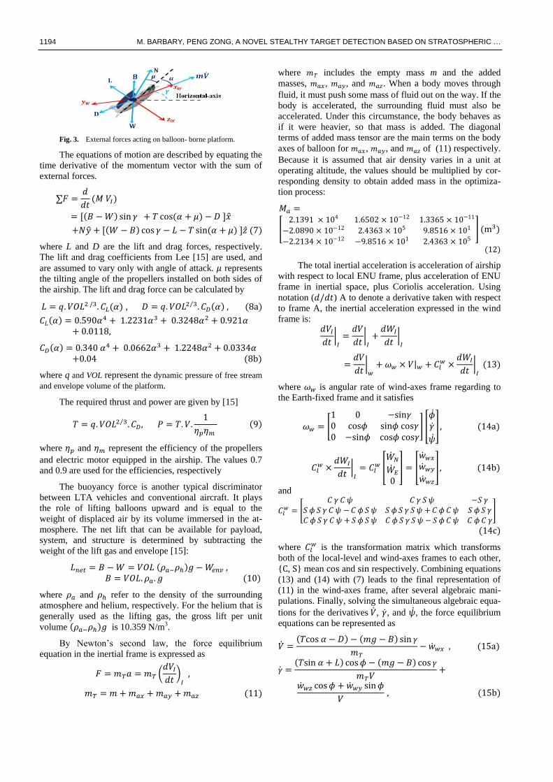
The Physical Optics (PO) Formula-3.
tion for Stealthy F-117A RCS Model
In the presence of a perfectly conducting surface, the
total electromagnetic field of a source may be expressed as
a superposition of the incident fields (𝐸𝑖 , 𝐻𝑖) and the fields (𝐸𝑠, 𝐻𝑠) which are scattered by the surface. The scattered
fields can be expressed in terms of the radiation integrals
over actual currents induced on the surface of the scatterer.
The PO assumes that the induced surface currents on the
scatterer surface are given by the geometrical optics (GO)
currents over those portions of the surface directly illumi-
nated by the incident magnetic field, �⃗⃗� 𝑖 , and zero over the
shadowed sections of the surface [16]:
𝐽𝑆⃗⃗⃗ = {2�̂� × �⃗⃗� 𝑖 , illuminated region0 , shadow region
(17)
where �̂� denotes the outward unit normal vector on a sur-
face. The authors in this paper use PO method to predict
RCS of a stealth target based on the geometry model of
F-117A, which are modeled by the triangular facets. The
geometry model of the stealth target based on F-117A is
approximated by a model consisting of many triangular
facets, in which there are a large number of points on the
surface described in terms of Cartesian coordinates. This
surface is then approximated by planar triangular facets
connecting these points. An arbitrary midpoint p of the
triangle surface is assigned coordinates (𝑟𝑝, 𝜃𝑝, 𝜙𝑝), the
observation point is assigned coordinates (𝑟𝑠 , 𝜃𝑠, 𝜙𝑠) and
unit vectors (�̂�𝑠 , �̂�𝑠, �̂�𝑠). Normal vector �̂� is a unit vector
with its tip at the midpoint of triangle. Then �̂� can be
expressed as cross product of vectors 𝐴𝐵⃗⃗⃗⃗ ⃗ and 𝐴𝐶⃗⃗⃗⃗ ⃗. Once
these vectors are found, �̂� can directly be found by
�̂� = 𝐴𝐵⃗⃗⃗⃗ ⃗ × 𝐴𝐶⃗⃗⃗⃗ ⃗ / |𝐴𝐵⃗⃗⃗⃗ ⃗||𝐴𝐶⃗⃗⃗⃗ ⃗|. These parameters are depicted in
Fig. 4.
Thus far, the discussion has involved the calculation
of the scattered field from a single facet. Superposition is
used to calculate the scattered field from the stealth target.
First, the scattered field is computed for each facet. Then,
the scattered field from each facet is vector summed to
produce the total field in the observation direction. If the
source is at a great distance from the target, it will illumi-
nate the target with an incident field which is essentially
a plane wave. The incident electric field intensity is given
by �⃗� 𝑖 = (𝐸𝑖𝜃�̂�𝑖 + 𝐸𝑖∅�̂�𝑖)𝑒−𝑗�⃗� 𝑖�̂�𝑖∙𝑟 𝑝, where 𝐸𝑖𝜃, 𝐸𝑖𝜙 are the
Fig. 4. Vector definitions of an approximation of a stealthy
F-117A model using triangular facets on the surface.
orthogonal components in terms of the variables θ and 𝜙,
(𝑟𝑖 , 𝜃𝑖 , 𝜙𝑖) are the spherical coordinates of the source and
(�̂�𝑖 , �̂�𝑖 , �̂�𝑖) are the unit vectors, so the magnetic field inten-
sity of the incident field is given by:
�⃗⃗� 𝑖 =�⃗� 𝑖 × �⃗� 𝑖𝑍0
=1
𝑍0(𝐸𝑖∅�̂�𝑖 − 𝐸𝑖𝜃�̂�𝑖)𝑒
𝑗�⃗� 𝑖ℎ (18)
where (𝑘 =2𝜋
𝜆), �⃗� 𝑖 is the propagation vector defined as
�⃗� 𝑖 = −𝑘(𝑥 sin 𝜃𝑖 cos 𝜙𝑖 + �̂� sin 𝜃𝑖 sin𝜙𝑖 + �̂� cos 𝜃𝑖) , 𝑍0 is
the intrinsic impedance of free space and ℎ = �̂�𝑖 ∙ 𝑟 𝑝
= 𝑥𝑝sin 𝜃𝑖 cos𝜙𝑖 + 𝑦𝑝 sin 𝜃𝑖 sin𝜙𝑖 +𝑧𝑝 cos 𝜃𝑖. Since radia-
tion integral for the scattered field is calculated by em-
ploying a GO approximation for the currents induced on
the surface, it can be concluded that PO is a high frequency
method, which implies that target is assumed to be electri-
cally large. For the scattered field, the vector potential is
given by [17]:
𝐴 =𝜇
4𝜋𝑟𝑠𝑒−𝑗𝑘𝑟𝑠∬𝐽 𝑠𝑒
𝑗𝑘�̂�𝑠∙𝑟 𝑝
𝑠
𝑑𝑠 (19)
where 𝜇 is the permeability of a specific medium. For a far-
field observation point, the following approximation holds
�⃗� 𝑠(𝑟𝑠, 𝜃𝑠, 𝜙𝑠)
= −𝑗𝑤𝐴
= −𝑗𝑤𝜇
2𝜋𝑟𝑠𝑒−𝑗𝑘𝑟𝑠∬�̂� × �⃗⃗� 𝑖𝑒
𝑗𝑘�̂�𝑠∙𝑟 𝑝
𝑠
𝑑𝑠
=𝑒−𝑗𝑘𝑟𝑠
𝑟𝑠(𝐸𝑖∅�̂�𝑖 − 𝐸𝑖𝜃�̂�𝑖) × (
𝑗
𝜆)∬�̂�𝑒𝑗𝑘(ℎ+𝑔)
𝑠
𝑑𝑠
⏟ 𝑠
(20)
where
𝑔 = �̂�𝑠 ∙ 𝑟 𝑝 = 𝑥𝑝 sin 𝜃𝑠 cos 𝜙𝑠 + 𝑦𝑝 sin 𝜃𝑠 sin𝜙𝑠 +𝑧𝑝 cos 𝜃𝑠.
However, it is not possible to obtain an exact closed form
solution for 𝑆 with this integral. Given that the incident
wavefront is assumed plane and the incident field is known
at the facet vertices, the amplitude and phase at the interior
integration points can be found by interpolation. Then, the
integrand can be expanded by using Taylor series, and each
term integrated to give a closed form result. Usually,
a small number of terms in Taylor series (on the order of 5)
will give a sufficiently accurate approximation with unit
amplitude plane wave (|Ei| = 1) [18].
1196 M. BARBARY, PENG ZONG, A NOVEL STEALTHY TARGET DETECTION BASED ON STRATOSPHERIC …
𝑆 = (𝑗
𝜆) |𝐴𝐵⃗⃗⃗⃗ ⃗ × 𝐴𝐶⃗⃗⃗⃗ ⃗| 𝑒𝑗𝐷0 {[
𝑒𝑗𝐷𝑝
𝐷𝑝(𝐷𝑞 − 𝐷𝑝)]
−[𝑒𝑗𝐷𝑞
𝐷𝑞(𝐷𝑞 − 𝐷𝑝)] −
1
𝐷𝑞𝐷𝑝} (21a)
where
𝐷𝑝 = 𝑘[(𝑥𝐵 − 𝑥𝐴) sin 𝜃𝑠 cos𝜙𝑠 + (𝑦𝐵 − 𝑦𝐴) sin 𝜃𝑠 sin𝜙𝑠
+(𝑧𝐵 − 𝑧𝐴) cos 𝜃𝑠 ], (21b)
𝐷𝑞 = 𝑘[(𝑥𝐶 − 𝑥𝐴) sin 𝜃𝑠 cos𝜙𝑠 + (𝑦𝐶 − 𝑦𝐴) sin 𝜃𝑠 sin𝜙𝑠
+(𝑧𝐶 − 𝑧𝐴) cos 𝜃𝑠] , (21c)
𝐷0 = 𝑘[𝑥𝐴 sin 𝜃𝑠 cos𝜙𝑠 + 𝑦𝐴 sin 𝜃𝑠 sin𝜙𝑠 + 𝑧𝐴 cos 𝜃𝑠].
(21d)
It is now possible to write the formula of PO current
as 𝐽 𝑠 = (𝐽𝑠𝑥 �̂� + 𝐽𝑠𝑦 �̂� + 𝐽𝑠𝑧�̂�)𝑒𝑗𝑘ℎ. In the general case, the
local facet coordinate system will not be aligned with the
global coordinate system. In the local facet coordinate
system (𝑥", 𝑦", 𝑧") , the facet lies on the 𝑥"𝑦" plane, with �̂�" being the normal to the facet surface, hence �̂� = �̂�". For any
arbitrary oriented facet with known global coordinates, its
local coordinates can be obtained by a series of two
rotations. First, angles α and β, are calculated by 𝛼 =
arctan[𝑛𝑦/𝑛𝑥] and 𝛽 = arccos (�̂� ∙ �̂�), where �̂� =
𝑛𝑥 �̂� + 𝑛𝑦 �̂� + 𝑛𝑧�̂�. The local coordinates can be trans-
formed to global coordinates [19]:
[𝑥"
𝑦"
𝑧"] = [
cos𝛽 0 − sin 𝛽0 1 0
sin 𝛽 0 cos𝛽] [cos 𝛼 sin𝛼 0− sin 𝛼 cos 𝛼 00 0 1
] [𝑥𝑦𝑧] (22)
However, in facet local coordinates, the surface cur-
rent does not have a �̂�"component, since the facet lies on
the 𝑥"𝑦"plane. Hence the local surface current is given by
𝐽 𝑠 = (𝐽′′𝑠𝑥 𝑥 ′′ + 𝐽′′
𝑠𝑦 �̂� ′′)𝑒𝑗𝑘ℎ, the surface current compo-
nents are [19]:
𝐽′′𝑠𝑥 = [𝐸"𝑖𝜃 cos𝜙
" cos 𝜃"
2𝑅𝑠 + 𝑍0 cos 𝜃"−
𝐸"𝑖𝜙 sin𝜙"
2𝑅𝑠 cos 𝜃" + 𝑍0
] cos 𝜃" (23a)
𝐽′′𝑠𝑦 = [𝐸"𝑖𝜃 sin𝜙
" cos 𝜃"
2𝑅𝑠 + 𝑍0 cos 𝜃"+
𝐸"𝑖𝜙 cos𝜙"
2𝑅𝑠 cos 𝜃" + 𝑍0
] cos 𝜃" (23b)
where 𝐸"𝑖𝜃, 𝐸"𝑖𝜙 are the components of the incident field in
the local facet coordinates, 𝜃", 𝜙" are the spherical polar
angles of the local coordinates and 𝑅𝑠 being the surface
resistivity of the facet material. When 𝑅𝑠 = 0, the surface is
a perfect electric conductor and assume that surface model
is smoothing. To obtain the total scattered field, simply
replace (23a) and (23b) in the radiation integral for the
triangular facet, which was determined in (21a), the total
number of facets (m = 20), so
�⃗� 𝑠(𝑟𝑠, 𝜃𝑠, 𝜙𝑠) = ∑−𝑗𝑘𝑍0𝑒
−𝑗(𝑘𝑟𝑠−𝐷0𝑚)
4𝜋𝑟𝑠
20
𝑚=1
(𝐽′′𝑠𝑚𝑥 𝑥′′ + 𝐽′′𝑠𝑚𝑦 �̂�
′′)
× |𝐴𝐵⃗⃗⃗⃗ ⃗𝑚 × 𝐴𝐶⃗⃗⃗⃗ ⃗𝑚| × {[𝑒𝑗𝐷𝑃𝑚
𝐷𝑃𝑚(𝐷𝑞𝑚 − 𝐷𝑃𝑚)]
− [𝑒𝑗𝐷𝑞𝑚
𝐷𝑞𝑚(𝐷𝑞𝑚 − 𝐷𝑃𝑚)] −
1
𝐷𝑞𝑚𝐷𝑃𝑚}. (24)
Once the scattered field is known, RCS is computed
in terms of the incident and scattered electric field intensi-
ties, and given by [20]:
𝑅𝐶𝑆(𝑟𝑠 , 𝜃𝑠, 𝜙𝑠) = lim𝑅→∞
4𝜋𝑅2|�⃗� 𝑠(𝑟𝑠, 𝜃𝑠, 𝜙𝑠)|
2
|�⃗� 𝑖|2 (25)
where R is the distance between the radar transmitter and
target. For most objects, radar cross section is a three-di-
mensional map of the scattering contributions, which varies
as a function of aspect angles (azimuth and elevation) and
polarization. The scattering matrix describes the scattering
behavior of a target as a function of polarization. Normally
it contains four RCS values (𝜃𝜃, 𝜃𝜙, 𝜙𝜃 and 𝜙𝜙), where
the first letter denotes the transmission polarization, the
second letter is the polarization at receive. Therefore, RCS
can be derived at any polarizations:
𝑅𝐶𝑆(𝑟𝑠, 𝜃𝑠, 𝜙𝑠) = lim𝑅→∞
4𝜋𝑅2 [|𝑆𝜃𝜃|
2 |𝑆𝜃𝜙|2
|𝑆𝜙𝜃|2|𝑆𝜙𝜙|
2] . (26)
The 𝑠𝑝𝑞 denotes the scattering parameter, whose first
subscript specifies polarization of the receive antenna and
the second one refers to polarization of the incident wave.
The elements of scattering matrix are complex quantities
and in terms of RCS [20]
𝑅𝐶𝑆𝑝𝑞 = 4𝜋𝑅2𝑆𝑝𝑞
2𝑒−2𝑗𝜓𝑝𝑞 ,
𝜓𝑝𝑞 = arctan
{
𝐼𝑚(𝐸𝑠𝑝𝐸𝑖𝑞)
𝑅𝑒(𝐸𝑠𝑝𝐸𝑖𝑞)}
. (27)
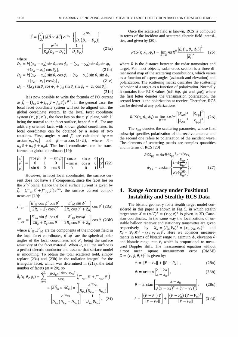
Range Accuracy under Positional 4.
Instability and Stealthy RCS Data
The bistatic geometry for a stealth target model con-
sidered in this paper is shown in Fig. 5, in which stealth
target state 𝑋 = (𝑝, 𝑉)𝑇 = (𝑥, 𝑦, 𝑧)𝑇 is given in 3D Carte-
sian coordinates. In the same way the localizations of un-
stable balloon receiver and stationary transmitter are given
respectively by 𝑋𝑅 = (𝑃𝑅, 𝑉𝑅)𝑇 = (𝑥𝑅 , 𝑦𝑅 , 𝑧𝑅)
𝑇 and
𝑋𝑇 = (𝑃𝑇 , 0)𝑇 = (𝑥𝑇 , 𝑦𝑇 , 𝑧𝑇)
𝑇. Here we consider measure-
ments in terms of bistatic range 𝑟, azimuth 𝜙, elevation 𝜃
and bistatic range–rate �̇�, which is proportional to meas-
ured Doppler shift. The measurement equation without
a root mean square measurement error (RMSE)
𝑍 = (𝑟, 𝜙, 𝜃, �̇�)𝑇 is given by:
𝑟 = ‖𝑃 − 𝑃𝑇‖ + ‖𝑃 − 𝑃𝑅‖ , (28a)
𝜙 = arctan [𝑦 − 𝑦𝑅𝑥 − 𝑥𝑅
] , (28b)
𝜃 = arctan [𝑧 − 𝑧𝑅
√(𝑥 − 𝑥𝑅)2 + (𝑦 − 𝑦𝑅)
2], (28c)
�̇� = [(𝑃 − 𝑃𝑇) 𝑉
‖𝑃 − 𝑃𝑇‖] + [
(𝑃 − 𝑃𝑅) (𝑉 − 𝑉𝑅)𝑇
‖𝑃 − 𝑃𝑅‖] (28d)
RADIOENGINEERING, VOL. 23, NO. 4, DECEMBER 2014 1197
Fig. 5. The stealthy target detection under positional
instability of balloon-borne bistatic radar system.
while the measurements at the receiver is characterized by
root mean square measurement error (RMSE) as
𝑟𝑚 = 𝑟 + 𝜎𝑅
𝜙𝑚 = 𝜙 + 𝜎𝜙 (29)
𝜃𝑚 = 𝜃 + 𝜎𝜃
The measurement accuracy is characterized by RMSE
of 𝜎𝑅, 𝜎𝜙, 𝜎𝜃 computed by three error components [21].
𝜎𝑅 = (𝜎𝑅𝑁2 + 𝜎𝑅𝐹
2 + 𝜎𝑅𝐵2)1/2 , (30a)
𝜎𝜙 = (𝜎𝜙𝑁2 + 𝜎𝜙𝐹
2 + 𝜎𝜙𝐵2)1/2 , (30b)
𝜎𝜃 = (𝜎𝜃𝑁2 + 𝜎𝜃𝐹
2 + 𝜎𝜃𝐵2)1/2 ( 30c)
where 𝜎𝑅𝑁 , 𝜎𝜙𝑁, 𝜎𝜃𝑁 are SNR dependent random range and
angular measurement errors, 𝜎𝑅𝐹 , 𝜎𝜙𝐹 , 𝜎𝜃𝐹 are range and
angular fixed errors, and 𝜎𝑅𝐵 , 𝜎𝜙𝐵, 𝜎𝜃𝐵 are range and angu-
lar bias errors. The SNR-dependent error usually dominates
the radar range angular errors, which are random with
a standard deviation and given by:
𝜎𝑅𝑁 =∆𝑅
√2(𝑆𝑁𝑅)=
𝐶
2𝐵√2(𝑆𝑁𝑅) , (31a)
𝜎𝜙𝑁 = 𝜎𝜃𝑁 =𝜃𝐵/ cos(𝜙 𝑜𝑟 𝜃)
𝐾𝑀√2(𝑆𝑁𝑅) (31b)
where B is the waveform bandwidth, C is the speed of light,
∆𝑅 is range resolution, 𝜃𝐵 is broadside beamwidth in the
angular coordinate of the measurement, and 𝐾𝑀 is mono-
pulse pattern difference slope, assuming the value of broad-
side beamwidth is 1° and 𝐾𝑀 is typically 1.6 [21]. The
bistatic form of radar equation is developed here to evalu-
ate bistatic radar sensitivity properties. The transmitter and
the receiver are deployed at two separate locations, either
or both of them changing with time. The receiver co-oper-
ates with transmitter through a synchronization link.
Normally, a co-located Tx and Rx are not described as a bi-
static system, even though they don’t share a common
antenna. Since the separation becomes significant relative
to the typical target range, so that bistatic radar systems
become relevant. It is also assumed that the target is an iso-
tropic radiator, giving a constant RCS in all directions.
Under these assumptions, it is reasonable to calculate bi-
static radar sensitivity by summing up the partial signal to
noise ratio as [2]:
𝑆𝑁𝑅 =𝑃𝑡𝐺𝑡𝐺𝑡𝑅𝐶𝑆𝐵𝜆
2
(4𝜋)3𝐾𝑇𝑠𝐵𝑛𝑅𝑡2𝑅𝑟
2𝐿 (32)
where 𝑃𝑡 is the peak transmitted power, 𝐺𝑡 is the transmit-
ter gain, 𝐺𝑟 is the receiver gain, 𝑅𝐶𝑆𝐵 is bistatic RCS of the
target, 𝜆 is the transmitted wavelength, 𝐵𝑛 is the bandwidth
of the transmitted waveform, k is Boltzmann’s constant, 𝑇𝑠 is the receiving system noise temperature, 𝐿 is the system
loss for transmitter and receiver, 𝑅𝑡 is the distance from the
transmitter to the target and 𝑅𝑟 is the distance from the
target to the receiver. Most of the previous researches in
bistatic radar systems only considered the simplest case of
bistatic radar sensitivity by isotropic radiator giving a con-
stant RCS in all directions except for the distance from the
transmitter and receiver to the target [3–8]. But this is not
an accurate consideration to calculate the SNR of stealth
target because the RCS value varies with elevation angle
and azimuth angles according to the position instability of
the balloon receiver. Therefore the accurate formula of
bistatic balloon-borne radar sensitivity depends on nature
RCS of stealth target and the position instability of the
balloon receiver, it should be written as:
𝑆𝑁𝑅𝐵(𝑟, 𝜙, 𝜃) = 𝑀 𝑅𝐶𝑆𝐵(𝑟, 𝜙, 𝜃)
𝑅𝑡2𝑅𝑟
2 , (33a)
𝑀 =𝑃𝑇𝐺𝑇𝐺𝑅𝜆
2
(4𝜋)3𝐾𝑇𝑠𝐵𝑛𝐿 . ( 33b)
From (33) and (31), the accurate form of random
range and angular measurement error SNR depend on RCS
of stealth target predicted by (PO) method in Section 3 and
are given by
𝜎𝑅𝑁 =𝐶
8𝐵√ 𝑀. 𝑅𝐶𝑆𝐵(𝑟, 𝜙, 𝜃)
𝑅𝑡2𝑅𝑟
2
, (34a)
𝜎𝜙𝑁 = 𝜎𝜃𝑁 =𝜃𝐵/ cos(𝜙 𝑜𝑟 𝜃)
𝐾𝑀√2(𝑀. 𝑅𝐶𝑆𝐵(𝑟, 𝜙, 𝜃)
𝑅𝑡2𝑅𝑟
2 )
. (34b)
By using the differential (29) and it can be expressed
in the matrix form [22]:
[𝑑𝑟𝑑𝜙𝑑𝜃
] =
[ 𝐶𝑅1 + 𝐶𝑇1 𝐶𝑅2 + 𝐶𝑇2 𝐶𝑅3 + 𝐶𝑇3
−𝑠𝑖𝑛2 𝜙
𝑦 − 𝑦𝑅
𝑐𝑜𝑠 2 𝜙
𝑥 − 𝑥𝑅0
𝐶𝑅3 𝑐𝑜𝑠 𝜙
𝑟𝑅−𝐶𝑅3 𝑠𝑖𝑛 𝜙
𝑟𝑅
𝑐𝑜𝑠 𝜃
𝑟𝑅 ]
[𝑑𝑥𝑑𝑦𝑑𝑧
] + [
𝑘𝑟𝑘𝜙𝑘𝜃
]
(35a)
where
𝐶𝑖1 =𝑥 − 𝑥𝑖𝑟𝑖
, 𝐶𝑖2 =𝑦 − 𝑦𝑖𝑟𝑖
, 𝐶𝑖3 =𝑧 − 𝑧𝑖𝑟𝑖
, 𝑖 = (𝑅, 𝑇), (35b)
𝑘𝑟 = −[𝐶𝑅1𝑑𝑥𝑅 + 𝐶𝑅2𝑑𝑦𝑅 + 𝐶𝑅3𝑑𝑧𝑅] , (35c)
𝑘𝜙 =𝑠𝑖𝑛2 𝜙
𝑦 − 𝑦𝑅𝑑𝑥𝑅 −
𝑐𝑜𝑠 2 𝜙
𝑥 − 𝑥𝑅𝑑𝑦𝑅 , (35d)

1198 M. BARBARY, PENG ZONG, A NOVEL STEALTHY TARGET DETECTION BASED ON STRATOSPHERIC …
𝑘𝜃 =𝐶𝑅3 𝑐𝑜𝑠 𝜙
𝑟𝑅𝑑𝑥𝑅 +
𝐶𝑅3 𝑠𝑖𝑛 𝜙
𝑟𝑅𝑑𝑦𝑅 +
𝑐𝑜𝑠 𝜃
𝑟𝑅𝑑𝑧𝑅 , (35e)
or 𝑑𝑉 = ℂ𝑑𝑋 + 𝑑𝑆 (36)
where ℂ (3×3) is the matrix of coefficients, 𝑑𝑋 (3×1) is
the vector of stealth target’s position error, 𝑑𝑉 (3×1) is the
vector measurement of stealth target’s position and
𝑑𝑆 (3×1) is the vector pertaining to all random
measurement error according to position instability of
balloon receiver. The solution of (36) is
𝑑𝑋 = ℂ−1(𝑑𝑋 − 𝑑𝑆). (37)
The corresponding covariance matrix of the stealthy
target position error is [22]:
𝑃𝑑𝑋 = ℂ−1{𝐸[𝑑𝑉𝑑𝑉𝑇] + 𝐸[𝑑𝑆𝑑𝑆𝑇]}ℂ−𝑇 . (38)
The expressions of 𝐸[𝑑𝑉𝑑𝑉𝑇] and 𝐸[𝑑𝑆𝑑𝑆𝑇] are given by
𝐸[𝑑𝑉𝑑𝑉𝑇] = diag[𝜎𝑟2 𝜎𝜙
2 𝜎𝜃2] , (39a)
𝐸[𝑑𝑆𝑑𝑆𝑇] =
[ 2 0 0
01
𝑟𝑅2 cos2 𝜃
(sin𝜙−cos𝜙) sin2𝜙sin𝜃
2𝑟𝑅
0(sin𝜙−cos𝜙) sin2𝜙 sin𝜃
2𝑟𝑅
1
𝑟𝑅2 ]
[
𝜎𝑥𝑅2
𝜎𝑦𝑅2
𝜎𝑧𝑅2
]
(39b)
where 𝜎𝑥𝑅 , 𝜎𝑦𝑅 , 𝜎𝑧𝑅 are the position instability measure-
ment errors of the balloon receiver
The RMSE is used to describe the stealthy target po-
sition accuracy, from (38), (39a) and (39b), it is noted that
the stealthy position accuracy is related to the position of
the considered target and the deployment of the two sites in
the bistatic system. So it is called GDOP (Geometrical
Dilution Of Position). The expression of the GDOP is [23]:
𝐺𝐷𝑂𝑃 = √𝑡𝑟 [𝑃𝑑𝑋] . (40)
The radar and target parameters are illustrated in
Tab. 1.
Parameter Value
𝑃𝑡(kWatt) 250
𝐺𝑡 , 𝐺𝑟 (dB) 32
f (MHz) 3000
𝐵𝑛 (MHz) 1
𝐿𝑡, 𝐿𝑟(dB) 5
𝜎𝑅𝐹(m) 3
𝜎𝑅𝐵 (m) 10
∆𝑅 (m) 10
𝜎𝜙𝐹(mrad) 0.2
𝜎𝜃𝐹(mrad) 0.2
𝜎𝜙𝐵(mrad) 0.5
𝜎𝜃𝐵(mrad) 0.5
V (m/s) 400
Tab. 1. The radar and stealthy target parameters.
Simulation Results 5.
5.1 Instability of Balloon-borne Receiver
according to Wind Speed Results
For all problems considered, the ideal balloon posi-
tion is fixed at (X = 150 km, Y = 100 km, Z = 21 km) from
the ground-based transmitter. The balloon is initialized by
flying at 1 m/s airspeed. With solving the optimal control
problems, we neglect the contribution from centripetal
acceleration, assuming acceleration is constant in the ENU
farm, with a magnitude of 0.029 m/s2. The simulation dis-
plays the positional instability of the balloon- borne re-
ceiver according to the horizontal wind speed, taking 250
seconds of random wind as an example, 𝜎𝑤 is of 15 m/s
shown in Fig. 6. It is clear that the mean wind velocity at
altitude of 21 km varies randomly between -15 to +15 m/s.
Fig. 7 shows the comparison between the ideal position and
unstable balloon position in X-direction and Y-direction. It
is clear that the balloon suspends in the stratosphere about
21 km above the Earth and extends in a sphere of 0.5 km
radius.
Fig. 6. Simulation of random horizontal wind speed.
0 50 100 150 200 250-15
-10
-5
0
5
10
15
20
Time (sec.)
Ho
rizo
nta
l w
ind
sp
ee
d (
m/s
)
W
E
WN
0 50 100 150 200 250
1.496
1.498
1.5
1.502
1.504
1.506x 10
5
Ba
llo
on
X-p
os
itio
n (
m)
time(s)
Unstable Balloon-borne X-position
Stable Balloon-borne X-position
0 50 100 150 200 2500.994
0.996
0.998
1
1.002
1.004
1.006
x 105
Ba
llo
on
Y-p
os
itio
n(m
)
time(s)
Unstable Balloon-borne Y-position
Stable Balloon-borne Y-position

RADIOENGINEERING, VOL. 23, NO. 4, DECEMBER 2014 1199
Fig. 7. The comparison between the ideal position and
unstable balloon position in X-direction and
Y-direction.
5.2 Establishing the Stealthy Target Model
and Stealthy RCS Results
Fig. 8(a) shows the geometry model and scatters of
stealth target F-117A in the range of (0 ≤ θ ≤ 360) and
(0 ≤ 𝜙 ≤ 360). Fig. 8(b) shows 3-D RCS of the stealth
target in bistatic system. A comparison of 2-D bistatic RCS
within different aspect angle θ according to the altitude of
bistatic receiver is demonstrated in Fig. 9(a). We further
assume that the incident wave is (θ-polarized), frequency is
3 GHz and elevation angle takes two values (θ = 80 and
120 degree) while azimuth angle 𝜙 between the horizon
and observation direction varies from (0 to 360 degrees). It
is clear that the RCS with a higher aspect angle in balloon-
borne radar is better than with lower aspect angles in
ground-based bistatic system. Fig. 9(b) shows the results in
2-D polar plot.
Fig. 8. Bistatic RCS of the stealthy target based on F-117A in
3-D.
(a)
(b)
Fig. 9. a) Comparison of RCS within different aspect angle θ
according to the altitude of bistatic receiver in 2-D,
b) the polar plot using different aspect angles.
5.3 SNR Results for Proposed Scheme under
Balloon Positional Instability & Stealthy
RCS
A comparison of radar sensitivity between the pro-
posed scheme in balloon-borne radar and conventional
ground-based bistatic system at X-direction is demon-
strated in Fig. 10. To clearly indicate SNR fluctuation of
real stealth target RCS in (X-axis) range, we assume that
the stealth target is moving at constant altitude 17 km and
constant velocity V = 400 m/s. Thus, as long as the range
changes, the elevation aspect angle changes similarly, say
the elevation angle 𝜃s = 180° for ground-based radar while
for balloon-borne radar 𝜃s = 0°, so as to satisfy the mini-
mum range between radar and stealth target. The maximum
range exists in the far field saturation, as elevation angle
𝜃s ≈ 90° for ground-based radar and 𝜃s ≈ 50° for balloon-
borne radar. Fig. 10 is a comparison between the SNR of
real stealth RCS subject to stable and unstable position of
the balloon-borne and flat RCS (0.025 m2) of conventional
ground-based system. It is clear that the sensitivity of the
proposed radar scheme has been improved due to increas-
ing scatterer RCS of stealth model with a higher aspect
angle comparing to the conventional system. The 3-D bi-
static radar sensitivities of taking flat RCS (0.025 m2) and
stealth RCS are shown in Fig. 11.
Fig. 10. A comparison between SNR for radar with real RCS of
a stealth target under stable and unstable balloon
position and ground-based system in X-direction.
-500 -400 -300 -200 -100 0 100 200 300 400 500 600-400
-300
-200
-100
0
100
200
300
400
500
y(m
)
x(m)
Balloon- borne Unstabe position ( X-Y plan )
Unstable position of Balloon
Ideal position of Balloon
-20
0
20
-20
0
20
-20
-10
0
10
20
Y(m)
3D RCS Plot of Stealth F117-A Model
X (m)
Z(m
)
(a)
-200
0
200
-200
0
200-100
-50
0
50
Elevation angle
(degree)
RCS of Stealth target model F-117A
Azimuth angle
(degree)
Ste
alth R
CS
(dB
)
-100
-80
-60
-40
-20
0
20
(b)
0 50 100 150 200 250 300 350
-30
-20
-10
0
10
20
30
40
Azimuth angle (degree)
Ste
alth
y R
CS
(d
Bsm
)
Stealthy RCS using balloon-borne radar(elevation angle=80°)
Stealthy RCS using ground based radar (elevation angle=120°)
0
10
20
30
30
210
60
240
90
270
120
300
150
330
180 0
-20
-10
0
10
20
30
30
210
60
240
90
270
120
300
150
330
180 0
-20
-10
0
10
20
30
30
210
60
240
90
270
120
300
150
330
180 0
-200 -150 -100 -50 0 50 100 150 200-40
-20
0
20
40
60
80
100
120
140
160
SN
R (
dB
)
X (Km)
SNR of monostatic Radar with Nature RCS of stealth target
Free space SNR using Ground-based radar with flat RCS (0.025m2)
Stealthy SNR using Balloon-borne radar with unstable position
Stealthy SNR using Balloon-borne radar with stable position
Stealthy SNR using Ground-based radar
Ground- receiver
𝜃 = 120 degree
Amid altitude receiver
𝜃 = 100 degree
Balloon receiver
𝜃= 80 degree
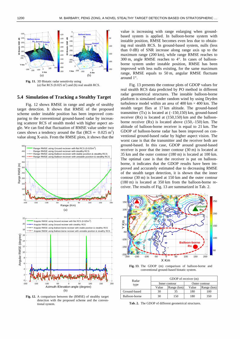
1200 M. BARBARY, PENG ZONG, A NOVEL STEALTHY TARGET DETECTION BASED ON STRATOSPHERIC …
(a) (b)
Fig. 11. 3D Bistatic radar sensitivity using
(a) flat RCS (0.025 m2) and (b) real stealth RCS.
5.4 Simulation of Tracking a Stealthy Target
Fig. 12 shows RMSE in range and angle of stealthy
target detection. It shows that RMSE of the proposed
scheme under instable position has been improved com-
paring to the conventional ground-based radar by increas-
ing scatterer RCS of stealth model with higher aspect an-
gle. We can find that fluctuation of RMSE value under two
cases shows a tendency around the flat (RCS = 0.025 m2)
value along X-axis. From the RMSE plots, it shows that the
(a)
(b)
Fig. 12. A comparison between the (RMSE) of stealthy target
detection with the proposed scheme and the conven-
tional system.
value is increasing with range enlarging when ground-
based system is applied. In balloon-borne system with
instable position, RMSE becomes even less due to obtain-
ing real stealth RCS. In ground-based system, nulls (less
than 0 dB) of SNR increase along range axis up to the
maximum range (200 km), while range RMSE reaches to
300 m, angle RMSE reaches to 4°. In cases of balloon-
borne system under instable position, RMSE has been
improved with less nulls existing, for the same maximum
range, RMSE equals to 50 m, angular RMSE fluctuate
around 1°.
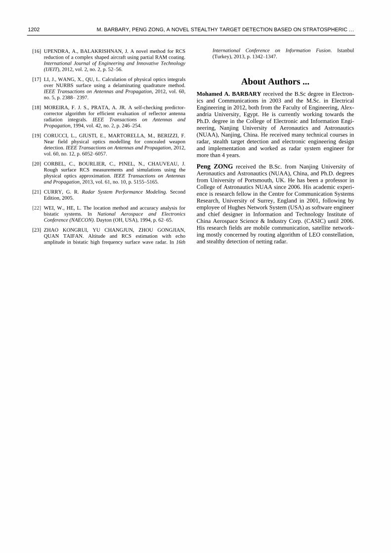
Fig. 13 presents the contour plots of GDOP values for
real stealth RCS data predicted by PO method in different
radar geometrical structures. The instable balloon-borne
platform is simulated under random wind by using Dryden
turbulence model within an area of 400 km × 400 km. The
stealth target flies at 17 km altitude. The ground-based
transmitter (Tx) is located at (–150,150) km, ground-based
receiver (Rx) is located at (150,150) km and the balloon-
borne receiver (Rx) is located above (150,–150) km. The
altitude of balloon-borne receiver is equal to 21 km. The
GDOP of balloon-borne radar has been improved on con-
ventional ground-based radar by higher aspect vision. The
worst case is that the transmitter and the receiver both are
ground-based. In this case, GDOP around ground-based
receiver is poor that the inner contour (30 m) is located at
35 km and the outer contour (180 m) is located at 100 km.
The optimal case is that the receiver is put on balloon-
borne, it indicates that the GDOP results have been im-
proved and accurately estimated due to decreasing RMSE
of the stealth target detection, it is shown that the inner
contour (30 m) is located at 150 km and the outer contour
(180 m) is located at 350 km from the balloon-borne re-
ceiver. The results of Fig. 13 are summarized in Tab. 2.
Fig. 13. The GDOP (m) comparison of balloon-borne and
conventional ground-based bistatic system.
Radar
type
GDOP of receiver (m)
Inner contour Outer contour
Value Range (km) Value Range (km)
Ground-based 30 35 180 100
Balloon-borne 30 150 180 350
Tab. 2. The GDOP of different geometrical structures.
-200 -100 0 100 200-200
0
200
-350
-300
-250
-200
-150
-100
X Km
3D
Bis
tati
c S
NR
d
B
-300
-280
-260
-240
-220
-200
-180
-160
-140
-120
Y Km
Ground
TxGround
Rx
Balloon-borne
Rx
-2000
200-200
0
200-300
-250
-200
-150
-100
-50
0
X KmY Km
3D
Bis
tati
c S
NR
d
B
-250
-200
-150
-100
-50
0
Balloon-borne
Rx
Ground
RxGround
Tx
-200 -150 -100 -50 0 50 100 150 200
0
50
100
150
200
250
300
350
400
450
500
Ra
ng
e R
MS
E (
m)
Range (Km)
Range RMSE using Ground reciever with flat RCS (0.025m2)
Range RMSE using Ground reciever with stealthy RCS
Range RMSE using Balloon reciever with stable position & stealthy RCS
Range RMSE using Balloon reciever with unstable position & stealthy RCS
-200 -150 -100 -50 0 50 100 150 200
0
2
4
6
8
10
12
14
16
18
20
22
An
gu
lar
RM
SE
(d
eg
ree
)
Azimuth /Elevation angle (degree)
Angular RMSE using Ground reciever with flat RCS (0.025m2)
Angular RMSE using Ground reciever with stealthy RCS
Angular RMSE using Balloon-borne reciever with stable position & stealthy RCS
Angular RMSE using Balloon-borne reciever with unstable position & stealthy RCS
30
30
30 3
0
30
30
3030
30
30
30
30
30
30
30
30
30
60
60
60
60
60
60
60
60
60
60
60
6060
60
60
60
6060
60
60
90
90
90
90
90
90
90
90
90
90
90
90
90
90
90
120
120
120
120
120
120
120
120
120
120 120
120
120
120
150
150
150
150
150
150 150 150
150
150
150
150
180
180
180
180
180
180 180
180
180
210
210 210
210
210
210
210
210
240
240
270
Y K
m
X Km
GDOP for Bistatic System with stealthy RCS (m)
-200 -150 -100 -50 0 50 100 150 200-200
-150
-100
-50
0
50
100
150
50
100
150
200
250
Balloon-borne
Rx
Tx Ground
Rx

RADIOENGINEERING, VOL. 23, NO. 4, DECEMBER 2014 1201
It is found that GDOP of the proposed scheme has been im-
proved due to decreasing the range and angular RMSE by
increasing scatterer RCS of the stealth model comparing to
the conventional ground-based system
In Fig. 14(a), the comparison between tracking of
stealth target using the proposed scheme under instable
position due to random wind speed and the conventional
ground system. It is clear that the position estimate error of
stealth target model was reduced by using the proposed
scheme at all time interval due to increasing stealth RCS
with a higher aspect vision as shown in Fig. 14(b).
(a)
Fig. 14. The comparison between the tracking of stealthy target
using balloon-borne bistatic system and conventional
ground-based bistatic system.
Conclusion 6.
An improvement of stealth RCS detection with higher
aspect vision is presented. The stratospheric balloon posi-
tional instability due to random wind is considered. The
results revealed that the proposed scheme demonstrates
higher location accuracy than the conventional ground-
based system. It is clear that bistatic radar sensitivity of the
proposed scheme has been improved due to increasing
scatterer RCS of stealth model with a higher aspect angle
as predicted by PO method. The comparison between
tracking of stealth target using the proposed scheme and
the conventional system is introduced. The GDOP of the
proposed scheme has been improved due to decreasing
RMSE of the balloon radar system comparing to the con-
ventional system. Finally the proposed system has better
performance at almost all time intervals.
Acknowledgments
This work is supported by the China National Found
of “863 Project”, Ref. 2013AA7010051.
References
[1] CHEN, X., GUAN, J., LIU, N., HE, Y. Maneuvering target
detection via Radon-Fractional Fourier transform-based long time
coherent integration. IEEE Trans. Signal Process, 2014, vol. 62,
no. 4, p. 939–953.
[2] TENG, Y., GRIFFITHS, H.D., BAKER, C.J., WOODBRIDGE, K.
Netted radar sensitivity and ambiguity. IET Radar Sonar Navig.,
December 2007, vol. 1, no. 6, p. 479–486.
[3] KUSCHEL, H., HECKENBACH, J., MULIER, ST., APPEL, R.
Countering stealth with passive, multi-static, low frequency radars.
IEEE Aerospace and Electronic Systems Magazine, 2010, vol.25,
no. 9, p. 11–17.
[4] KUSCHEL, H., HECKENBACH, J., MULIER, ST., APPEL, R.
On the potentials of passive, multistatic, low frequency radars to
counter stealth and detect low flying targets. In IEEE Conference,
RADAR '08, 2008, p. 1–6.
[5] HOWE, D. Introduction to the basic technology of stealthy
aircraft: Part 2- Illumination by the enemy (active considerations).
Journal of Engineering for Gas Turbines and Power, 1991,
vol. 113, no. 1, p. 80–86.
[6] EL-KAMCHOUCHY, H., SAADA, K., HAFEZ, A. Optimum
stealthy aircraft detection using a multistatic radar. ICACT
Transactions on Advanced Communications Technology (ICACT-
TACT), 2013, vol. 6, no. 2, p. 337–342.
[7] DENG, H. Orthogonal netted radar systems. IEEE Aerospace and
Electronic Systems Magazine, 2012, vol. 27, no. 5, p. 28–35.
[8] BEZOUSEK, P., SCHEJBAL, V. Bistatic and multistatic radar
systems. Radioengineering, 2008, vol. 17, no. 3, p. 53–59.
[9] AXIOTIS, D. I., THEOLOGOU, M. E., SYKAS, E. D. The effect
of platform instability on the system level performance of HAPS
UMTS. IEEE Communications Letters, 2004, vol. 8, no. 2, p. 111
to 113.
[10] BEAL, T. R. Digital simulation of atmospheric turbulence for
Dryden and von Karman models. Journal of Guidance, Control,
and Dynamics, 1993, vol. 16, no. 1, p. 132–138.
[11] FORTUNATI, S., FARINA, A., GINI, F., GRAZIANO, A.,
GRECO, M. S., GIOMPAPA, S. Impact of flight disturbances on
airborne radar tracking. IEEE Transactions on Aerospace and
Electronic Systems, 2012, vol. 48, no. 3, p. 2698 –2710.
[12] HOGGE, E. B-737 linear autoland simulink model. NASA,
Technical Report NASA/CR-2004-213021, 2004.
[13] MIELE, A., WANG, T., MELVIN, W. W. Optimal take-off
trajectories in the presence of wind shear. Journal of Optimization
Theory and Applications, 1986, vol. 49, no. 1, p. 1–45.
[14] FELDMAN, M. A. Efficient low-speed flight in a wind field.
Master Thesis. Blacksburg, VA, Virginia Polytechnic Inst. and
State Univ., July 1996.
[15] LEE, S., BANG, H. Three-dimensional ascent trajectory optimiza-
tion for stratospheric airship platforms in the jet stream. Journal of
Guidance, Control, and Dynamics, 2007, vol. 30, no. 5, p. 1341 to
1352.
-100
-50
0
50
100
-100
-50
0
50
100
0
5
10
15
20
Z K
m
True position of stealthy target
Ground station Tx
ideal Balloon- borne position
unstable Balloon - borne position
Ground station Rx
Ground Radar stealthy tracking
Unstable Balloon- borne stealthy tracking
Stable Balloon- borne stealthy tracking
Rx
Txy Km
x Km
balloon
0 2 4 6 8 10 12 14 16 18 200
100
200
300
time interval (sec)
Bis
tatic
RM
SE
(m
)
using Bistatic Balloon-borne radar system
using Bistatic Ground-based radar system
(b)
1202 M. BARBARY, PENG ZONG, A NOVEL STEALTHY TARGET DETECTION BASED ON STRATOSPHERIC …
[16] UPENDRA, A., BALAKRISHNAN, J. A novel method for RCS
reduction of a complex shaped aircraft using partial RAM coating.
International Journal of Engineering and Innovative Technology
(IJEIT), 2012, vol. 2, no. 2, p. 52–56.
[17] LI, J., WANG, X., QU, L. Calculation of physical optics integrals
over NURBS surface using a delaminating quadrature method.
IEEE Transactions on Antennas and Propagation, 2012, vol. 60,
no. 5, p. 2388– 2397.
[18] MOREIRA, F. J. S., PRATA, A. JR. A self-checking predictor-
corrector algorithm for efficient evaluation of reflector antenna
radiation integrals. IEEE Transactions on Antennas and
Propagation, 1994, vol. 42, no. 2, p. 246–254.
[19] CORUCCI, L., GIUSTI, E., MARTORELLA, M., BERIZZI, F.
Near field physical optics modelling for concealed weapon
detection. IEEE Transactions on Antennas and Propagation, 2012,
vol. 60, no. 12, p. 6052–6057.
[20] CORBEL, C., BOURLIER, C., PINEL, N., CHAUVEAU, J.
Rough surface RCS measurements and simulations using the
physical optics approximation. IEEE Transactions on Antennas
and Propagation, 2013, vol. 61, no. 10, p. 5155–5165.
[21] CURRY, G. R. Radar System Performance Modeling. Second
Edition, 2005.
[22] WEI, W., HE, L. The location method and accuracy analysis for
bistatic systems. In National Aerospace and Electronics
Conference (NAECON). Dayton (OH, USA), 1994, p. 62–65.
[23] ZHAO KONGRUI, YU CHANGJUN, ZHOU GONGJIAN,
QUAN TAIFAN. Altitude and RCS estimation with echo
amplitude in bistatic high frequency surface wave radar. In 16th
International Conference on Information Fusion. Istanbul
(Turkey), 2013, p. 1342–1347.
About Authors ...
Mohamed A. BARBARY received the B.Sc degree in Electron-
ics and Communications in 2003 and the M.Sc. in Electrical
Engineering in 2012, both from the Faculty of Engineering, Alex-
andria University, Egypt. He is currently working towards the
Ph.D. degree in the College of Electronic and Information Engi-
neering, Nanjing University of Aeronautics and Astronautics
(NUAA), Nanjing, China. He received many technical courses in
radar, stealth target detection and electronic engineering design
and implementation and worked as radar system engineer for
more than 4 years.
Peng ZONG received the B.Sc. from Nanjing University of
Aeronautics and Astronautics (NUAA), China, and Ph.D. degrees
from University of Portsmouth, UK. He has been a professor in
College of Astronautics NUAA since 2006. His academic experi-
ence is research fellow in the Centre for Communication Systems
Research, University of Surrey, England in 2001, following by
employee of Hughes Network System (USA) as software engineer
and chief designer in Information and Technology Institute of
China Aerospace Science & Industry Corp. (CASIC) until 2006.
His research fields are mobile communication, satellite network-
ing mostly concerned by routing algorithm of LEO constellation,
and stealthy detection of netting radar.


