
_____________________________
A Reactive Planning Approach for
Demand-Driven Wood
Remanufacturing Industry: A
Real-Scale Application
Rezvan Rafiei Mustapha Nourelfath Jonathan Gaudreault Luis Antonio Santa-Eulalia Mathieu Bouchard November 2012 CIRRELT-2012-71
G1V 0A6
Bureaux de Montréal : Bureaux de Québec :
Université de Montréal Université Laval C.P. 6128, succ. Centre-ville 2325, de la Terrasse, bureau 2642 Montréal (Québec) Québec (Québec) Canada H3C 3J7 Canada G1V 0A6 Téléphone : 514 343-7575 Téléphone : 418 656-2073 Télécopie : 514 343-7121 Télécopie : 418 656-2624
www.cirrelt.ca
A Reactive Planning Approach for Demand-Driven Wood Remanufacturing Industry: A Real-Scale Application
Rezvan Rafiei1,2,*, Mustapha Nourelfath1,2, Jonathan Gaudreault1,3, Luis Antonio Santa-Eulalia4, Mathieu Bouchard 1,2
1 Interuniversity Research Centre on Enterprise Networks, Logistics and Transportation (CIRRELT)
2 Department of Mechanical Engineering, Université Laval, Pavillon Adrien-Pouliot, 1065, avenue de la médecine, Québec, Canada G1V 0A6
3 Department of Computer Science and Software Engineering, Université Laval, Pavillon Adrien-Pouliot, 1065, avenue de la médecine, Québec, Canada G1V 0A6
4 School of Applied Sciences, University of Campinas, rua Pedro Zaccaria, 1300, 13484-350, Limeira, São Paulo, Brazil
Abstract. Managing uncertainty is one of the main challenges within the forest supply
chain. This paper studies a wood remanufacturing mill that experiences important
disruptions due to uncertain demands. In order to handle these demands, a mathematical
programming model is sketched as a baseline to provide a reactive planning strategy
using a periodic policy. By changing the objective function of this baseline model, several
approaches are selected. The effectiveness of the reactive planning strategy is then
illustrated, and the impact of the selected approaches is evaluated, considering planning
period length and planning time window. Various comparisons are made among
approaches based on backorder levels and cost values. The experiments results based
on this real-scale industrial case show that backorder quantity can be minimized but a
huge cost. However the trade-off between backorder and cost can be established.
Keywords. Reactive planning, uncertain demand, wood remanufacturing industry, mixed
integer programming, simulation.
Acknowledgements. The authors would like to thank the Natural Sciences and
Engineering Research Council of Canada (NSERC) for financial support.
Results and views expressed in this publication are the sole responsibility of the authors and do not necessarily reflect those of CIRRELT.
Les résultats et opinions contenus dans cette publication ne reflètent pas nécessairement la position du CIRRELT et n'engagent pas sa responsabilité. _____________________________
* Corresponding author: [email protected]
Dépôt légal – Bibliothèque et Archives nationales du Québec Bibliothèque et Archives Canada, 2012
© Copyright Rafiei, Nourelfath, Gaudreault, Santa-Eulalia, Bouchard and CIRRELT, 2012

1. Introduction
One of the fundamental aspects that a manufacturing system faces is that uncertain demands increase the
complexity of the manufacturing processes. Most industries are confronted with varying customer
demands for different products. The performance of a plan in “pull” systems (wherein demands from
customers are taken into account) is very sensitive to demand fluctuations, and it is not trivial to
efficiently adjust the production plan to changes. As a result of demand fluctuations, the production
process outputs and inputs become different from the planned quantities. In fact, over or underestimating
uncertain demands and its side effects could lead to inefficient production plans as well as loss of market
share (Gupta and Maranas 2003). Therefore, a particularly challenging problem for mills is to make
decisions under uncertainty in demands.
Many existing papers use a stochastic programming (SP) approaches to manage uncertainties.
The SP method expresses uncertainties as probability density functions. Unfortunately, uncertainties will
not be predictable if no information exists about their behaviour. Under conditions that uncertainty level
is important and the data follows no known probability distribution, reactive planning approaches have
been recommended by many researches (e.g., Li and Ierapetritou 2008 and Lou et al. 2012). This
approach generates an on-line plan which makes decisions locally in real-time. Reactive actions can take
place at the edge of fixed intervals of time or when uncertainties unfold. In both situations, the plan is
updated based on the new upcoming information.
This study is motivated by a real-scale case in a wood remanufacturing industry. Uncertainty of
demands is a key problem in this mill and has a major influence on its processes. It is in fact very
difficult for managers to adequately handle these unpredictable demands. Any pre-computed or
predictive plan inevitably requires continuous updates to quickly react to disturbances from the business
milieu, which can be costly. In a remanufacturing unit (e.g., bed frame components manufacturing),
managers are obliged to review the production plans daily due to the arrival of new and unexpected
orders from clients. In practice, this is handled through manual approaches by supply chain planners,
A Reactive Planning Approach for Demand-Driven Wood Remanufacturing Industry: A Real-Scale Application
CIRRELT-2012-71 1
who usually rely mostly on their experience and intuition. It is quite hard for them to efficiently manage
the large quantity of information from the complex business environment in order to be sure that their
adapted plans are really cost-efficient. That is, when demand goes up, planners are not able to have a
swift reaction to demand change and decide whether to lose sale or to encounter a stock-out. It is likely
that either the customer will go to elsewhere or the mill will pay a backorder penalty. This issue is
aggravated by a co-production system wherein multiple types of finished products are produced at the
same time from a single raw material. In co-production systems with a finite production capacity a given
demand may face with backorder, because other products mostly with smaller market demand and high
inventory level are simultaneously produced. Therefore, production planning is a complex procedure in
this mill by having a co-production system together with highly uncertain demands. Decreasing the
backorder quantity to reach a high service level is a challenging problem for this wood remanufacturing
mill. The present paper presents a reactive planning strategy to help managers for making decisions
about how to deal swiftly with uncertain demands.
Following these introductory remarks, a literature review is given and the paper contribution is
highlighted in Section 2. A case in wood remanufacturing industry will be described in Section 3. In
Section 4, a mathematical programming model is developed. Then, considering different kinds of
disturbances of this initial plan, an efficient re-planning strategy is proposed and validated by simulation
in Section 5. Finally, conclusions are drawn in Section 6.
2. Literature review
Various types of uncertainty may be encountered in a manufacturing environment. Such uncertainties
according to the characteristics and resources can be distinguished as one of three types (Lou et al.
2012): 1) Complete unknown uncertainties which are unpredictable events, such as a sudden accident,
strike, or similar. 2) Suspicious uncertainties about the future, which are not easy to quantify, for
example, rush order arrivals, order cancellations, machine breakdowns and demand fluctuations. 3)
Known uncertainties are those about which some information is available, for example, processing times
A Reactive Planning Approach for Demand-Driven Wood Remanufacturing Industry: A Real-Scale Application
2 CIRRELT-2012-71
and demand with known probability distributions.
No advance information is available about complete unknown uncertainties so developing a plan
is hard in this condition. They are beyond the scope of the current work. Preventive scheduling generates
scheduling policy before the uncertainty occurs. It is also often applied when the uncertainty can be
quantified in some way (Li and Ierapetritou 2008). Therefore it can deal with known uncertainties.
Planning approaches such as stochastic programming, robust optimization methods, fuzzy programming
methods, and sensitivity analysis were identified in known uncertainties category (Li and Ierapetritou
2008). This kind of planning generates an off-line plan which is executed regardless of events occurring
after its formation. A new schedule would not be constructed before the complete execution of the
current plan (Wan 1995).
There is not enough information in advance for realization of suspicious uncertainties about the
future parameters. Therefore, the reactive planning approach is followed in which a plan is generated or
modified when decisions are made locally in real-time. In fact it generates an on-line plan that will
allow a protective action. The on-line planning practice makes decisions using either a complete reactive
planning or a predictive–reactive (repair) planning approach. Complete reactive planning regenerates a
new plan from scratch and decisions are made locally in real-time whereas predictive–reactive planning
is a process to repair or modify the preventive plan. In this case, the reactive planning is in fact
complementary to the preventive planning to respond to suspicious uncertainties about the future. An
interesting debate among researchers is to select between predictive–reactive, or complete reactive
rescheduling. This issue is stated by Sabuncuoglu and Bayiz (2000), Sun and Xue (2001), Cowling and
Johansson (2002), Vieira et al. (2003), Aytug et al. (2005) and Ouelhadj and Petrovic (2009). Sun and
Xue (2001) recommended to revise only part of the original plan whereas Aytug et al. (2005) believed if
there is little uncertainty in manufacturing environment, predictive–reactive methods are highly likely to
provide better plans, than complete reactive approaches.
Another controversial issue is about when to use rescheduling strategy in the presence of
suspicious uncertainties about the future. Periodic policy, event-driven policy, and hybrid policy are
A Reactive Planning Approach for Demand-Driven Wood Remanufacturing Industry: A Real-Scale Application
CIRRELT-2012-71 3
distinguished as rescheduling policies (Vieira et al. 2003, Aytug et al. 2005, Ouelhadj and Petrovic
2009). From the perspective of the authors, periodic policy defines a regular interval between
rescheduling actions while rescheduling actions are not allowed during each interval. In event-driven
policy, rescheduling action is triggered when events with higher potential of disruption to the system
happen. A hybrid policy reschedules the system periodically as well as when an exception event takes
place. In the following some of recent studies will be presented.
Duenas and Petrovic (2008) developed a predictive schedule with uncertain material shortage in
parallel machines scheduling problem. Also, Gholami and Zandieh (2009) presented a hybrid scheduling
for a flow shop with sequence dependent setup times and machines with random breakdowns. In recent
years, Frantzen et al. (2011) used a predictive-reactive approach, where rescheduling was executed
periodically. They also applied a complete reactive approach to support the work of the production
planner by regenerating feasible schedules when required. The approach presented by Lou et al. (2012)
applied a proactive–reactive scheduling for job shops to handle uncertainties in dynamic manufacturing
environments. In the proactive scheduling stage, their objective was to generate a robust predictive
schedule against known uncertainties. In the reactive scheduling stage, the objective was to modify the
predictive schedule to adapt to suspicious uncertainties about the future.
As mentioned in the literature, one of the fundamental issues in the re-planning strategy is the
approach selection. If there is little uncertainty in demand, a predictive–reactive approach is
recommended otherwise a complete re-planning approach has a better performance. In our case, a
complete re-planning approach is applied to take into account the high uncertainty in demand. The other
issue is when the selected approach has to be used. Selection of re-planning policy depends on the
previous plan, for example an event–driven policy often has a good performance when a predictive plan
exists in advance. We focus on the periodic policy, because there is no predictive plan in this case and
we decided not to build one. Moreover the periodic policy yields more plan stability (Ouelhadj and
Petrovic 2009)
A Reactive Planning Approach for Demand-Driven Wood Remanufacturing Industry: A Real-Scale Application
4 CIRRELT-2012-71
The purpose of this paper is to prescribe for the forest industry on how to improve the current
practices, and on how to plan and re-plan efficiently the supply chain under uncertain demands using a
periodic complete re-planning approach. Many researches have been applied a reactive scheduling using
one of the approaches and policies defined in the literature at the operational level. In general, the
majority of this works generates a new schedule or modifies the exiting schedule and compares that with
the initial one by specific performance measures. We did not find any research explaining how a
complete re-planning approach by periodic policy works at the operational planning level, especially for
the wood manufacturing industry. This paper fills this gap by proposing a planning/re-planning strategy.
This process involves the interplay between generating a plan by an optimization approach, and the
impact of different values of re-planning period length and planning time window on this plan. A
simulation model then is needed to evaluate the impact of different values of systemic parameters in the
production planning. This study considers four optimization approaches, eight levels of re-planning
frequency, and seven levels of planning time window in a real-scale industrial case. A simulation model
is developed to compare the performance of different approaches in various re-planning configurations
by calibrating that against the real-world data from a wood remanufacturing mill which is described in
the next section.
3. Industrial case: a remanufacturing mill
Our industrial case is a wood remanufacturing mill in Eastern Canada. In this mill, the production
planning system involves processes of lumber sorting, lumber drying, and remanufacturing. Lumber
remanufacturing is a secondary business that generates value added products to be used in specialized
applications. This mill uses the defective lumbers which are transported from different sawmills. They
can be green or dried lumbers and have already been categorized based on the Canadian lumber grading
rules and standards. These graded lumbers are classified again consistent with home-made grade rules in
the mill. Green lumbers will be dried to reach appropriate moisture content. The remanufacturing
process, thus, adds value to dried lumbers through new cuts, grades and packaging. These final products
A Reactive Planning Approach for Demand-Driven Wood Remanufacturing Industry: A Real-Scale Application
CIRRELT-2012-71 5
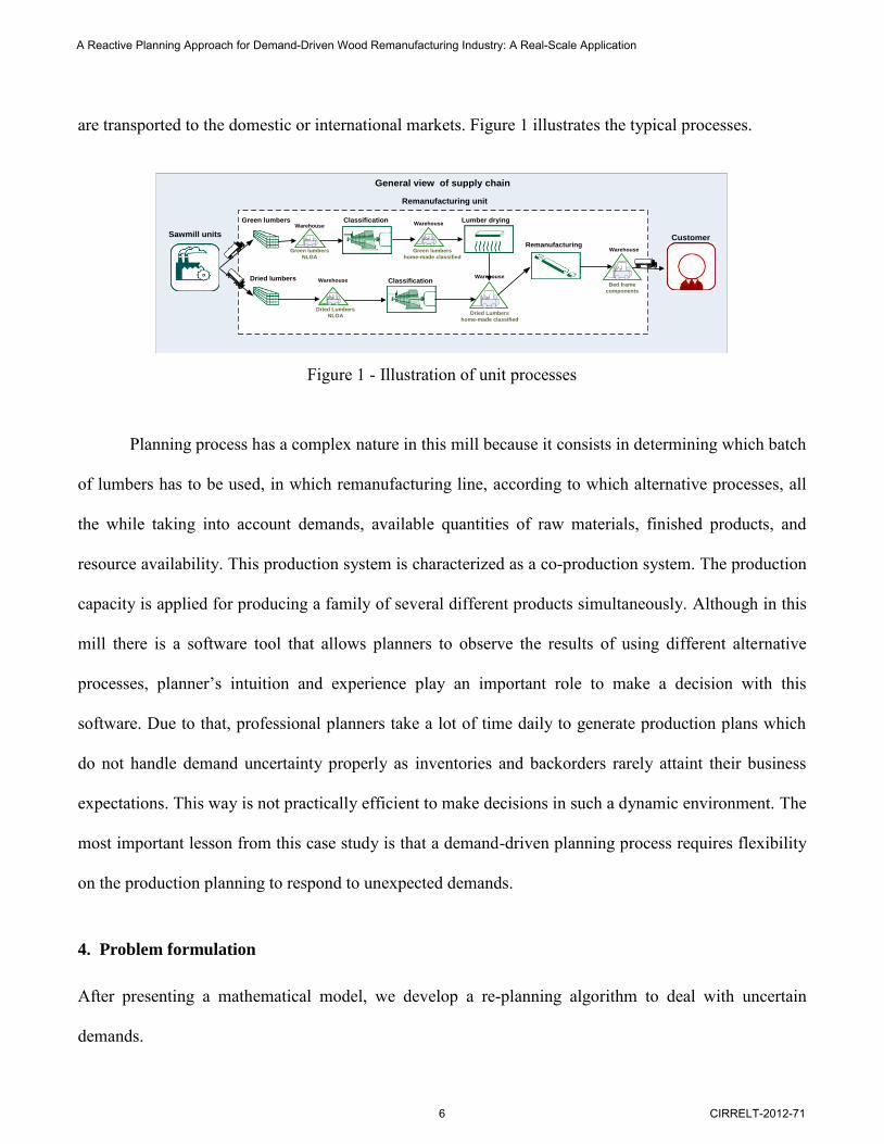
are transported to the domestic or international markets. Figure 1 illustrates the typical processes.
Sawmill units
Green lumbers
Dried lumbers
Classification
Classification
Lumber drying
Remanufacturing
Warehouse
WarehouseWarehouse
Warehouse
Warehouse
Green lumbers
NLGA
Green lumbers
home-made classified
Dried Lumbers
NLGADried Lumbers
home-made classified
Bed frame
components
Customer
Remanufacturing unit
General view of supply chain
Figure 1 - Illustration of unit processes
Planning process has a complex nature in this mill because it consists in determining which batch
of lumbers has to be used, in which remanufacturing line, according to which alternative processes, all
the while taking into account demands, available quantities of raw materials, finished products, and
resource availability. This production system is characterized as a co-production system. The production
capacity is applied for producing a family of several different products simultaneously. Although in this
mill there is a software tool that allows planners to observe the results of using different alternative
processes, planner’s intuition and experience play an important role to make a decision with this
software. Due to that, professional planners take a lot of time daily to generate production plans which
do not handle demand uncertainty properly as inventories and backorders rarely attaint their business
expectations. This way is not practically efficient to make decisions in such a dynamic environment. The
most important lesson from this case study is that a demand-driven planning process requires flexibility
on the production planning to respond to unexpected demands.
4. Problem formulation
After presenting a mathematical model, we develop a re-planning algorithm to deal with uncertain
demands.
A Reactive Planning Approach for Demand-Driven Wood Remanufacturing Industry: A Real-Scale Application
6 CIRRELT-2012-71

4.1 The mathematical model
Consider a production unit with a set of consumedP , producedP , and R . A planning horizon consisting of
T periods with the index t that refers to periods 1,...,t T .
4.1.1 Notations
Sets
consumedP Products p that can be consumed producedP Products p that can be produced
R Set of recipes r (A recipe is called an alternative process)
Parameters
rmc
Marginal contribution of recipe r that is the marginal profit of all products
producedp P to be produced simultaneously using recipe r (Note that it
includes the production costs)
pti
Inventory holding cost per unit of products producedp P in period t
ptbo
Backorder cost per unit of product producedp P in period t
sc
Cost for changing a setup
rtc Production costs associated with using recipe r in period t (This parameter is
used when the marginal contribution is not considered)
r
Capacity required for each recipe r per unit time
tsc
Setup time needed to changeover between recipes
tc
Available capacity of machine for period t (number of time units)
0pic
The inventory of raw material consumedp P at the beginning of planning
horizon
pts Supply of raw material consumedp P provided at the beginning of period t
pr The units of raw material consumedp P consumed by recipe r
0pip
The inventory of product producedp P at the beginning of planning horizon
pr The quantity of product producedp P produced by recipe r
ptd Demand of product producedp P to be delivered by the end of period t
A Reactive Planning Approach for Demand-Driven Wood Remanufacturing Industry: A Real-Scale Application
CIRRELT-2012-71 7

Decision variables rtX Number of times each recipe r should be run in period t
rtZ Binary setup variable, 1 if there is a machine changeover for recipe r at
period t. 0 otherwise
ptIC Inventory size of raw material consumedp P by the end of period t
ptIP Inventory size of product producedp P by the end of period t
ptBO Backorder size of product producedp P by the end of period t
4.1.2 The mixed integer programming (MIP) model
The objective function has an essential role in production planning optimization problems which may
have a remarkable influence on the model efficiency. As previously mentioned, the goal is to reduce the
amount of backorder. Hence many possible alternative objective functions are considered in the
following four different approaches.
The first approach consists in minimizing the sum of backorder quantities. Hence, the objective
function of Approach 1 is:
produced
T
ptt p P
Minimize BO
(1)
The second approach consists in maximizing the “marginal contribution”, which is calculated as
the prices of finished products minus their total variable costs of production and consumed raw
materials. Marginal contribution can determine the profitability of individual products or a family of
products. In addition, an essential part of obtaining an appropriate cost function is taking into account
the products holding costs, backorder costs and setup costs. Therefore, the objective function of
Approach 2 is:
A Reactive Planning Approach for Demand-Driven Wood Remanufacturing Industry: A Real-Scale Application
8 CIRRELT-2012-71
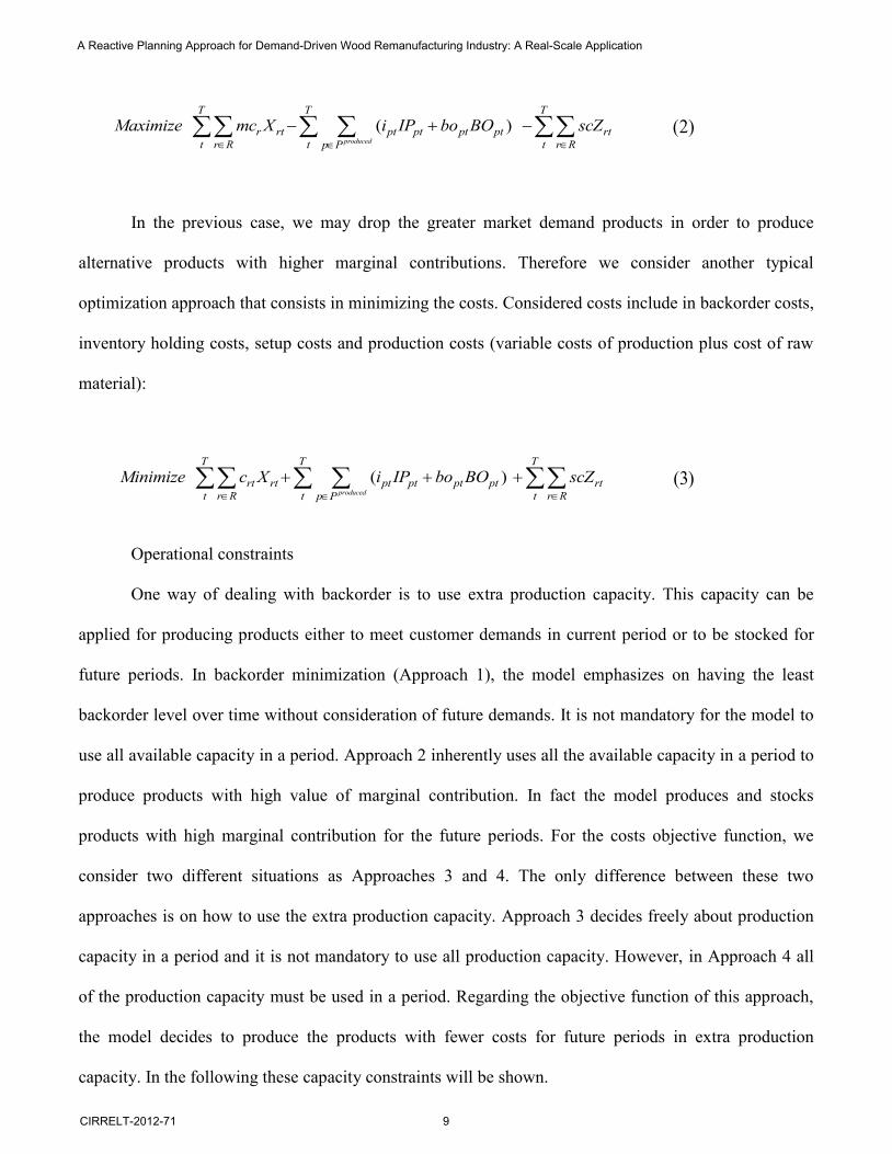
( )produced
T T T
r rt pt pt pt pt rtt r R t t r Rp P
Maximize mc X i IP bo BO scZ
(2)
In the previous case, we may drop the greater market demand products in order to produce
alternative products with higher marginal contributions. Therefore we consider another typical
optimization approach that consists in minimizing the costs. Considered costs include in backorder costs,
inventory holding costs, setup costs and production costs (variable costs of production plus cost of raw
material):
( )produced
T T T
rt rt pt pt pt pt rtt r R t t r Rp P
Minimize c X i IP bo BO scZ
(3)
Operational constraints
One way of dealing with backorder is to use extra production capacity. This capacity can be
applied for producing products either to meet customer demands in current period or to be stocked for
future periods. In backorder minimization (Approach 1), the model emphasizes on having the least
backorder level over time without consideration of future demands. It is not mandatory for the model to
use all available capacity in a period. Approach 2 inherently uses all the available capacity in a period to
produce products with high value of marginal contribution. In fact the model produces and stocks
products with high marginal contribution for the future periods. For the costs objective function, we
consider two different situations as Approaches 3 and 4. The only difference between these two
approaches is on how to use the extra production capacity. Approach 3 decides freely about production
capacity in a period and it is not mandatory to use all production capacity. However, in Approach 4 all
of the production capacity must be used in a period. Regarding the objective function of this approach,
the model decides to produce the products with fewer costs for future periods in extra production
capacity. In the following these capacity constraints will be shown.
A Reactive Planning Approach for Demand-Driven Wood Remanufacturing Industry: A Real-Scale Application
CIRRELT-2012-71 9
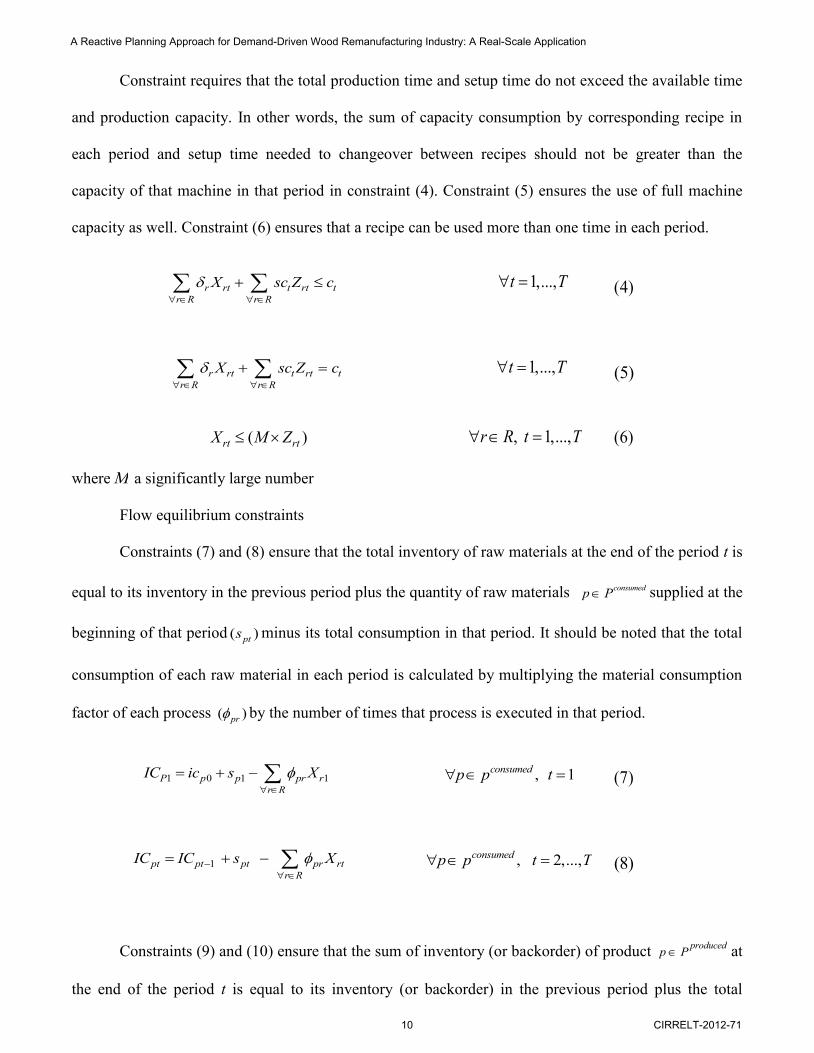
Constraint requires that the total production time and setup time do not exceed the available time
and production capacity. In other words, the sum of capacity consumption by corresponding recipe in
each period and setup time needed to changeover between recipes should not be greater than the
capacity of that machine in that period in constraint (4). Constraint (5) ensures the use of full machine
capacity as well. Constraint (6) ensures that a recipe can be used more than one time in each period.
r rt t rt tr R r R
X sc Z c
1,...,t T (4)
r rt t rt tr R r R
X sc Z c
1,...,t T (5)
( )rt rtX M Z
, 1,...,r R t T
(6)
where M a significantly large number
Flow equilibrium constraints
Constraints (7) and (8) ensure that the total inventory of raw materials at the end of the period t is
equal to its inventory in the previous period plus the quantity of raw materials consumedp P supplied at the
beginning of that period ( )pts minus its total consumption in that period. It should be noted that the total
consumption of each raw material in each period is calculated by multiplying the material consumption
factor of each process ( )pr by the number of times that process is executed in that period.
1 0 1 1P p p pr rr R
IC ic s X
, 1consumedp p t (7)
1pt pt pt pr rtr R
IC IC s X
, 2,...,consumedp p t T (8)
Constraints (9) and (10) ensure that the sum of inventory (or backorder) of product producedp P at
the end of the period t is equal to its inventory (or backorder) in the previous period plus the total
A Reactive Planning Approach for Demand-Driven Wood Remanufacturing Industry: A Real-Scale Application
10 CIRRELT-2012-71
production of that product in that period, minus the product demand for that period. Total quantity of
production for each product in each period is calculated by multiplying the production factor of each
recipe ( )pr by the number of times that recipe is executed in that period. Note that in this paper demand
is considered as a hard constraint.
1 1 0 1 1p P p pr r pr R
IP BO ip X d
, 1producedp P t (9)
1 1pt pt pt pt pr rt ptr R
IP BO IP BO X d
, 2,...,producedp p t T (10)
Finally, constraints (11)-(13) enforce the non-negativity and binary restriction on the decision
variables.
Non-negative and binary variables:
0, 0,1rt rtX Z
, 1,...,r R t T (11)
0ptIC , 1,...,consumedp P t T (12)
0, 0pt ptIP BO , 1,...,producedp P t T (13)
4.1.3 Approaches of the MIP model
The proposed MIP model is a baseline to provide different approaches which will be used
independently to evaluate the suggested re-planning strategy. Table 1 shows these approaches.
A Reactive Planning Approach for Demand-Driven Wood Remanufacturing Industry: A Real-Scale Application
CIRRELT-2012-71 11

Table 1: Approaches of the MIP model
Approaches Objective function Constraints
Approach 1: Min Backorder quantity Equation 1 Equations 4,6-13 Approach 2: Max Marginal contribution Equation 2 Equations 4,6-13 Approach 3: Min Costs Equation 3 Equations 4,6-13 Approach 4: Min Costs + Full capacity Equation 3 Equations 5,6-13
Some assumptions make the foundation of this MIP model. The drying activities of the mill are
not considered in the model. Note that machine reconfiguration (setup) for switching from one recipe to
another recipe is constant. Also no limitation is considered on supply of raw materials.
4.2 The re-planning approach
To include the real-time nature of demand variations in the production planning, we applied the MIP
model for a complete re-planning approach with periodic policy.
We define some expressions that are used in this paper. In the planning horizon the beginning
period is considered as the Initial period and the ending period is considered as the final period. Time
Step (TS) is the re-planning period length. Time Window (TW) is the planning time window. In a TW,
the beginning period is the first period and its ending period is the end period. The time between the first
and the end period in a TW is considered as an interval. The first and end period of the next interval are
obtained by adding TS to the first and the end period of the current interval.
Upcoming information
Upcoming information
Upcoming information
Upcoming information
P1 P2 P3 P4 P5
Plan1
P3 P4 P5 P6 P7
Plan2
P5 P6 P7 P8 P9
Plan3
P7 P8 P9 P10 P11
Plan4
P9 P10 P11 P12 P13
Plan5
Initial information
Complete re-planning approach by Periodic policy
Final information
Initial period =P1 Final period=P10 Time Step=2 Periods Time Window=5 periods Planning horizon=10 Periods
first-period end-periodInterval 1
TWTS
Figure 2: Illustration of complete re-planning approach by periodic policy
A Reactive Planning Approach for Demand-Driven Wood Remanufacturing Industry: A Real-Scale Application
12 CIRRELT-2012-71

In Figure 2 an example is illustrated about how the complete re-planning approach by the
periodic policy works. This figure shows representative problem instances during 10 periods. Here the
initial period is the period 1st and the final period is the period 10th. TS of example is equal to 2 periods
that results in revising the plan every two periods and for the total of 5 times. Here, TW is equal to 5
periods. The initial information, such as initial inventory of raw materials, and finished products, will be
the input data of the first interval. Plan1 makes a decision in the first interval based on the relevant
information for 5 periods. The output of plan1, such as inventory of raw materials, backorders, and
finished products quantities at the end of period 2 will be the input of the second interval. This procedure
continues until the final period.
From the perspective of the periodic complete re-planning strategy, re-planning is carried out as
an algorithm in Figure 3. Before starting the algorithm TS and TW have to be defined. In lines (1) the
primary setting for the initial and final periods are determined. The first and end periods are defined in
lines (2:3). Lines (4:11) are a loop to solve the model in the current interval until the final period is
reached. Line (5) sets the current interval. The model is executed for the current interval on line 6. In
lines (7:8) the result of the current interval is transferred to the next interval as the initial data. Lines
(9:10) add TS to the first and end periods to obtain the next interval. Line 4 is the stopping criterion.
When all periods are covered, the algorithm is terminated with success, otherwise continues for new
interval.
A Reactive Planning Approach for Demand-Driven Wood Remanufacturing Industry: A Real-Scale Application
CIRRELT-2012-71 13
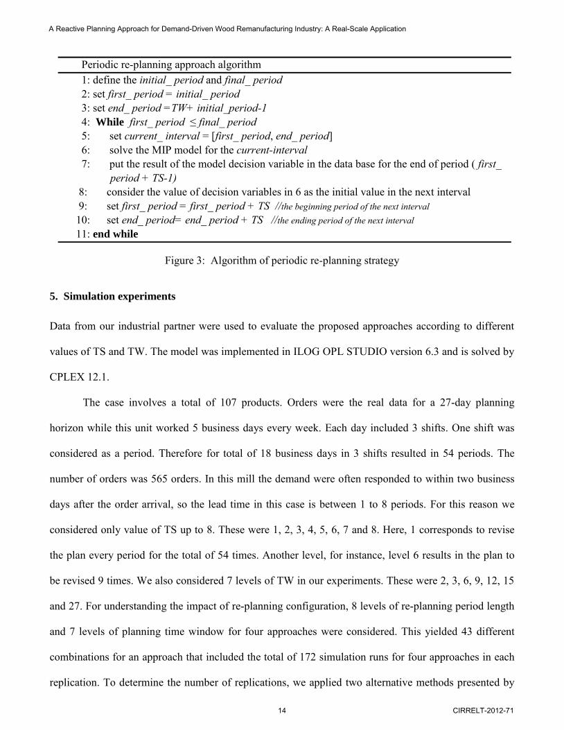
Figure 3: Algorithm of periodic re-planning strategy
5. Simulation experiments
Data from our industrial partner were used to evaluate the proposed approaches according to different
values of TS and TW. The model was implemented in ILOG OPL STUDIO version 6.3 and is solved by
CPLEX 12.1.
The case involves a total of 107 products. Orders were the real data for a 27-day planning
horizon while this unit worked 5 business days every week. Each day included 3 shifts. One shift was
considered as a period. Therefore for total of 18 business days in 3 shifts resulted in 54 periods. The
number of orders was 565 orders. In this mill the demand were often responded to within two business
days after the order arrival, so the lead time in this case is between 1 to 8 periods. For this reason we
considered only value of TS up to 8. These were 1, 2, 3, 4, 5, 6, 7 and 8. Here, 1 corresponds to revise
the plan every period for the total of 54 times. Another level, for instance, level 6 results in the plan to
be revised 9 times. We also considered 7 levels of TW in our experiments. These were 2, 3, 6, 9, 12, 15
and 27. For understanding the impact of re-planning configuration, 8 levels of re-planning period length
and 7 levels of planning time window for four approaches were considered. This yielded 43 different
combinations for an approach that included the total of 172 simulation runs for four approaches in each
replication. To determine the number of replications, we applied two alternative methods presented by
Periodic re-planning approach algorithm 1: define the initial_ period and final_ period 2: set first_ period = initial_ period 3: set end_ period =TW+ initial_period-1 4: While first_ period ≤ final_ period 5: set current_ interval = [first_ period, end_ period] 6: solve the MIP model for the current-interval 7: put the result of the model decision variable in the data base for the end of period ( first_
period + TS-1) 8: consider the value of decision variables in 6 as the initial value in the next interval 9: set first_ period = first_ period + TS //the beginning period of the next interval 10: set end_ period= end_ period + TS //the ending period of the next interval 11: end while
A Reactive Planning Approach for Demand-Driven Wood Remanufacturing Industry: A Real-Scale Application
14 CIRRELT-2012-71
Itami et al. (2005) to obtain 90% confidence intervals. The results showed that more than 35 replications
were needed. Thus, for each approach, 40 replications were performed to get average estimations on
performance measures with 90% confidence intervals.
5.1 Data analysis
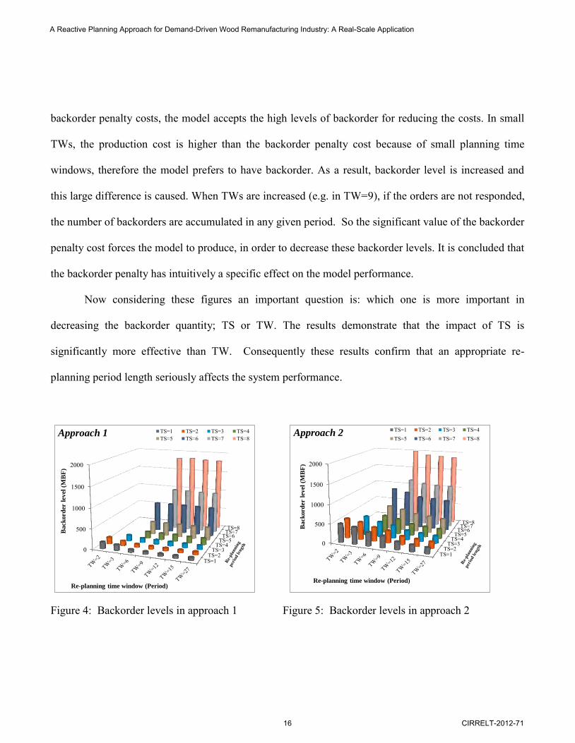
The results are presented in Figures 4-7 and Tables 2-5. In Figures 4, 5, 6, and 7, backorder levels in
simulation experiments are shown for different approaches. The minimum level of backorder belongs to
Approach 1 that is shown in Figure 4 because the only purpose of this approach is to decrease backorder
quantity without considering the costs values. In an interval the model avoids to postpone orders to the
future intervals as long as production capacity allows. After Approach 1, Approach 4 has the minimum
level of backorder in most of the cases (see Figure 7). In this approach, although the model uses all the
production capacity to satisfy current demands and to predict future demands, the backorder level is
almost three times that of Approach 1 in small TSs. The reason of this difference is that this approach
focuses on the costs reduction, therefore in addition to decreasing the backorder level the costs values
also have to be controlled by the model. Figure 5 shows that Approach 2 competes with Approach 4 in
the amount of backorders, and it has even better results in a few experiments. Approach 2 has acceptable
results and has a significant difference with highest level of backorder in Approach 3. In the second
approach the model applies all the available production capacity to meet demands. Demands should be
prepared by alternative processes that have the maximum value of production among others whereas one
alternative process needs a specific production time to produce a group of products. In this approach,
variation in the required time and profit margins of the alternative processes will result in the higher
level of backorder compare to other mentioned approaches. Approach 3 has much higher level of
backorder that is shown in Figure 6. This figure shows the backorder quantity of different experiments in
this approach up to 2000 MBF, but there are a lot more experiments with the values more than 2000 that
have not been shown in this figure. The behaviour of the backorder level in Approach 3 is more
informative. This approach is very sensitive to costs values so when the production costs are more than
A Reactive Planning Approach for Demand-Driven Wood Remanufacturing Industry: A Real-Scale Application
CIRRELT-2012-71 15
backorder penalty costs, the model accepts the high levels of backorder for reducing the costs. In small
TWs, the production cost is higher than the backorder penalty cost because of small planning time
windows, therefore the model prefers to have backorder. As a result, backorder level is increased and
this large difference is caused. When TWs are increased (e.g. in TW=9), if the orders are not responded,
the number of backorders are accumulated in any given period. So the significant value of the backorder
penalty cost forces the model to produce, in order to decrease these backorder levels. It is concluded that
the backorder penalty has intuitively a specific effect on the model performance.
Now considering these figures an important question is: which one is more important in
decreasing the backorder quantity; TS or TW. The results demonstrate that the impact of TS is
significantly more effective than TW. Consequently these results confirm that an appropriate re-
planning period length seriously affects the system performance.
Figure 4: Backorder levels in approach 1 Figure 5: Backorder levels in approach 2
TS=1TS=2
TS=3TS=4
TS=5TS=6
TS=7TS=8
0
500
1000
1500
2000
Back
ord
er l
evel
(MB
F)
Re-planning time window (Period)
Approach 1 TS=1 TS=2 TS=3 TS=4TS=5 TS=6 TS=7 TS=8
TS=1TS=2
TS=3TS=4
TS=5TS=6
TS=7TS=8
0
500
1000
1500
2000
Back
ord
er l
evel
(MB
F)
Re-planning time window (Period)
Approach 2 TS=1 TS=2 TS=3 TS=4TS=5 TS=6 TS=7 TS=8
A Reactive Planning Approach for Demand-Driven Wood Remanufacturing Industry: A Real-Scale Application
16 CIRRELT-2012-71
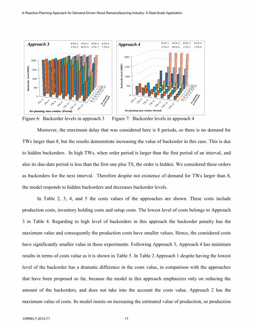
Figure 6: Backorder levels in approach 3 Figure 7: Backorder levels in approach 4
Moreover, the maximum delay that was considered here is 8 periods, so there is no demand for
TWs larger than 8, but the results demonstrate increasing the value of backorder in this case. This is due
to hidden backorders. In high TWs, when order period is larger than the first period of an interval, and
also its due-date period is less than the first one plus TS, the order is hidden. We considered these orders
as backorders for the next interval. Therefore despite not existence of demand for TWs larger than 8,
the model responds to hidden backorders and decreases backorder levels.
In Table 2, 3, 4, and 5 the costs values of the approaches are shown. These costs include
production costs, inventory holding costs and setup costs. The lowest level of costs belongs to Approach
3 in Table 4. Regarding to high level of backorders in this approach the backorder penalty has the
maximum value and consequently the production costs have smaller values. Hence, the considered costs
have significantly smaller value in these experiments. Following Approach 3, Approach 4 has minimum
results in terms of costs value as it is shown in Table 5. In Table 2 Approach 1 despite having the lowest
level of the backorder has a dramatic difference in the costs value, in comparison with the approaches
that have been proposed so far, because the model in this approach emphasizes only on reducing the
amount of the backorders, and does not take into the account the costs value. Approach 2 has the
maximum value of costs. Its model insists on increasing the estimated value of production, so production
TS=1TS=2
TS=3TS=4
TS=5TS=6
TS=7TS=8
0
500
1000
1500
2000
Back
ord
er
level
(M
BF
)
Re-planning time window (Period)
Approach 3 TS=1 TS=2 TS=3 TS=4TS=5 TS=6 TS=7 TS=8
TS=1TS=2
TS=3TS=4
TS=5TS=6
TS=7TS=8
0
500
1000
1500
2000
Back
ord
er l
evel
(M
BF
)
Re-planning time window (Period)
Approach 4 TS=1 TS=2 TS=3 TS=4TS=5 TS=6 TS=7 TS=8
A Reactive Planning Approach for Demand-Driven Wood Remanufacturing Industry: A Real-Scale Application
CIRRELT-2012-71 17
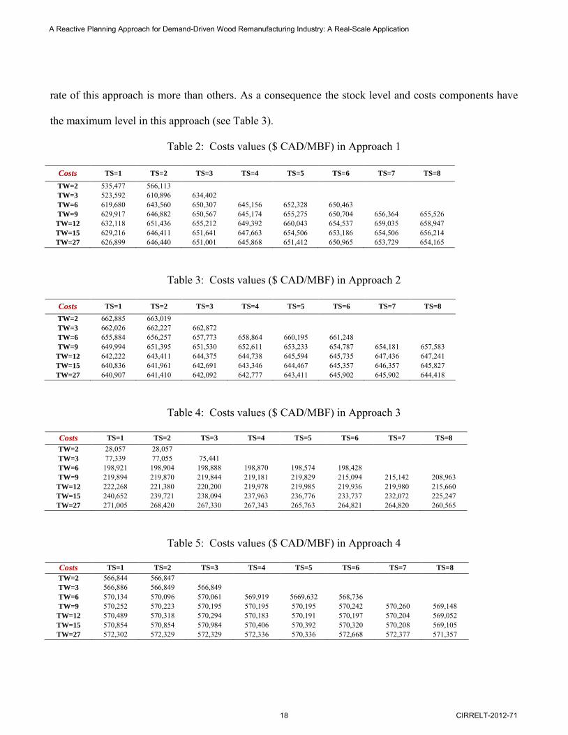
rate of this approach is more than others. As a consequence the stock level and costs components have
the maximum level in this approach (see Table 3).
Table 2: Costs values ($ CAD/MBF) in Approach 1
Costs TS=1 TS=2 TS=3 TS=4 TS=5 TS=6 TS=7 TS=8
TW=2 535,477 566,113 TW=3 523,592 610,896 634,402 TW=6 619,680 643,560 650,307 645,156 652,328 650,463 TW=9 629,917 646,882 650,567 645,174 655,275 650,704 656,364 655,526
TW=12 632,118 651,436 655,212 649,392 660,043 654,537 659,035 658,947 TW=15 629,216 646,411 651,641 647,663 654,506 653,186 654,506 656,214 TW=27 626,899 646,440 651,001 645,868 651,412 650,965 653,729 654,165
Table 3: Costs values ($ CAD/MBF) in Approach 2
Costs TS=1 TS=2 TS=3 TS=4 TS=5 TS=6 TS=7 TS=8
TW=2 662,885 663,019 TW=3 662,026 662,227 662,872 TW=6 655,884 656,257 657,773 658,864 660,195 661,248 TW=9 649,994 651,395 651,530 652,611 653,233 654,787 654,181 657,583
TW=12 642,222 643,411 644,375 644,738 645,594 645,735 647,436 647,241 TW=15 640,836 641,961 642,691 643,346 644,467 645,357 646,357 645,827 TW=27 640,907 641,410 642,092 642,777 643,411 645,902 645,902 644,418
Table 4: Costs values ($ CAD/MBF) in Approach 3
Costs TS=1 TS=2 TS=3 TS=4 TS=5 TS=6 TS=7 TS=8
TW=2 28,057 28,057 TW=3 77,339 77,055 75,441 TW=6 198,921 198,904 198,888 198,870 198,574 198,428 TW=9 219,894 219,870 219,844 219,181 219,829 215,094 215,142 208,963
TW=12 222,268 221,380 220,200 219,978 219,985 219,936 219,980 215,660 TW=15 240,652 239,721 238,094 237,963 236,776 233,737 232,072 225,247 TW=27 271,005 268,420 267,330 267,343 265,763 264,821 264,820 260,565
Table 5: Costs values ($ CAD/MBF) in Approach 4
Costs TS=1 TS=2 TS=3 TS=4 TS=5 TS=6 TS=7 TS=8
TW=2 566,844 566,847 TW=3 566,886 566,849 566,849 TW=6 570,134 570,096 570,061 569,919 5669,632 568,736 TW=9 570,252 570,223 570,195 570,195 570,195 570,242 570,260 569,148
TW=12 570,489 570,318 570,294 570,183 570,191 570,197 570,204 569,052 TW=15 570,854 570,854 570,984 570,406 570,392 570,320 570,208 569,105 TW=27 572,302 572,329 572,329 572,336 570,336 572,668 572,377 571,357
A Reactive Planning Approach for Demand-Driven Wood Remanufacturing Industry: A Real-Scale Application
18 CIRRELT-2012-71
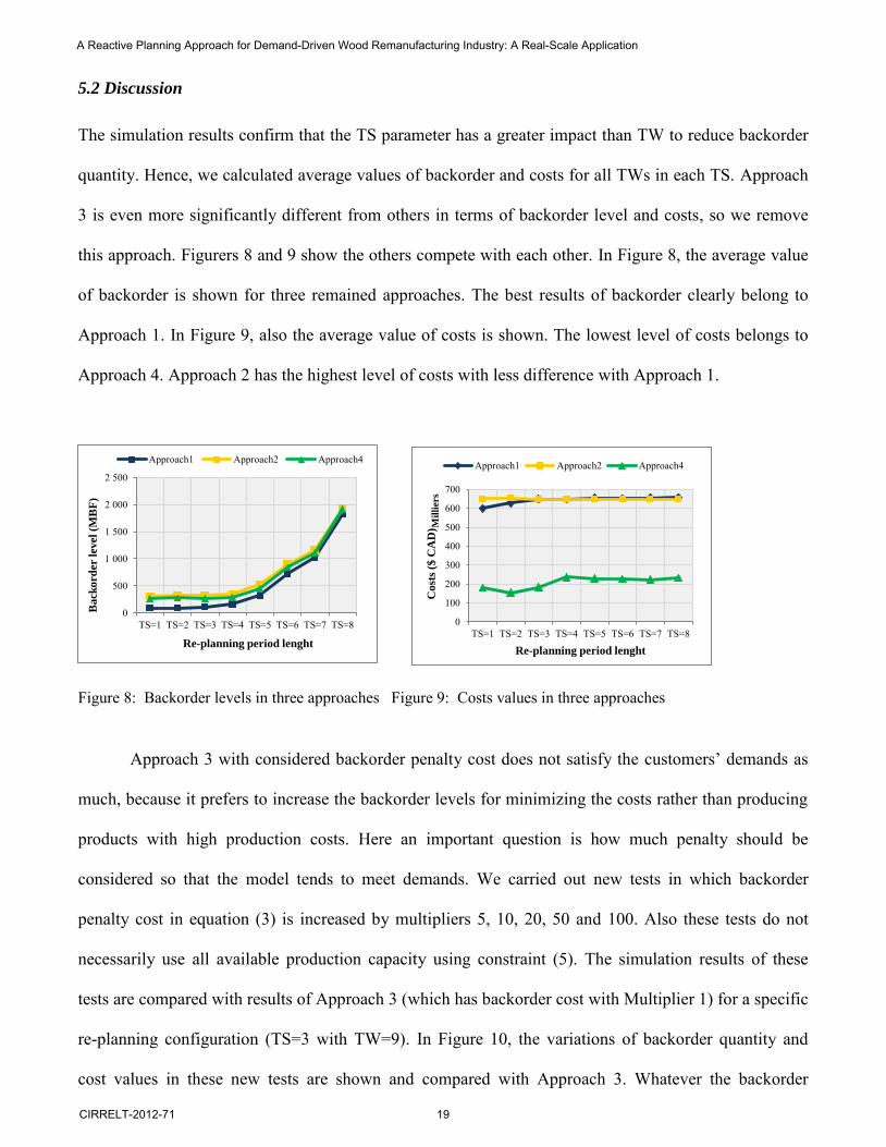
5.2 Discussion
The simulation results confirm that the TS parameter has a greater impact than TW to reduce backorder
quantity. Hence, we calculated average values of backorder and costs for all TWs in each TS. Approach
3 is even more significantly different from others in terms of backorder level and costs, so we remove
this approach. Figurers 8 and 9 show the others compete with each other. In Figure 8, the average value
of backorder is shown for three remained approaches. The best results of backorder clearly belong to
Approach 1. In Figure 9, also the average value of costs is shown. The lowest level of costs belongs to
Approach 4. Approach 2 has the highest level of costs with less difference with Approach 1.
Figure 8: Backorder levels in three approaches Figure 9: Costs values in three approaches
Approach 3 with considered backorder penalty cost does not satisfy the customers’ demands as
much, because it prefers to increase the backorder levels for minimizing the costs rather than producing
products with high production costs. Here an important question is how much penalty should be
considered so that the model tends to meet demands. We carried out new tests in which backorder
penalty cost in equation (3) is increased by multipliers 5, 10, 20, 50 and 100. Also these tests do not
necessarily use all available production capacity using constraint (5). The simulation results of these
tests are compared with results of Approach 3 (which has backorder cost with Multiplier 1) for a specific
re-planning configuration (TS=3 with TW=9). In Figure 10, the variations of backorder quantity and
cost values in these new tests are shown and compared with Approach 3. Whatever the backorder
0
500
1 000
1 500
2 000
2 500
TS=1 TS=2 TS=3 TS=4 TS=5 TS=6 TS=7 TS=8
Ba
ck
ord
er l
evel
(MB
F)
Re-planning period lenght
Approach1 Approach2 Approach4
0
100
200
300
400
500
600
700
TS=1 TS=2 TS=3 TS=4 TS=5 TS=6 TS=7 TS=8
Co
sts
($ C
AD
) Mil
liers
Re-planning period lenght
Approach1 Approach2 Approach4
A Reactive Planning Approach for Demand-Driven Wood Remanufacturing Industry: A Real-Scale Application
CIRRELT-2012-71 19

quantity decreases conversely the costs value increases. The least value of the backorder belongs to
Multiplier 100. Note that this value is less than 200 and it is even better than the value of Approach 4 in
terms of backorder. The most value of the cost among the approaches belongs to Multiplier 100 as well.
Note that this value is less than 500,000 and it has even better result than Approach 4 in terms of costs.
Figure 10: Comparison of backorder levels in new tests vs. Approach 3
The simulation results of these new tests and Approach 3 are also compared with results of
Approach 1 as a benchmark because it has the minimum value of backorder. In Figure 11, the variations
of backorder quantity and cost values are shown to compare these new tests with Approach 1.
Figure 11: Comparison of backorder levels in new tests vs. Approaches 1 and 3– for all costs
components
Although Approach 1 has the lowest level of backorder and it is even better than Multipliers
100 and 50, its cost is more than the others. As a consequence, if the model is not forced to use all the
0
100000
200000
300000
400000
500000
600000
0
500
1000
1500
2000
1 5 10 20 50 100
Co
st (
$C
AD
)
Ba
ck
ord
er q
ua
nti
ty (
MB
F)
Backorder cost multiplier
Backorder QTY and costs value in Approach 3 vs. new tests
Backorder QTY Costs
0 200 400 600 800 1000 1200 1400 1600 1800 2000
0 100 000 200 000 300 000 400 000 500 000 600 000 700 000
Approach 1
Approach 3
Multiplier 5
Multiplier 10
Multiplier 20
Multiplier 50
Multiplier 100
Backorder quantity (MBF)
Costs ($ CAD)
Costs
Backorder QTY
A Reactive Planning Approach for Demand-Driven Wood Remanufacturing Industry: A Real-Scale Application
20 CIRRELT-2012-71
available time, it has to have a high level of backorder penalty in this case, otherwise it tends to have
backorder.
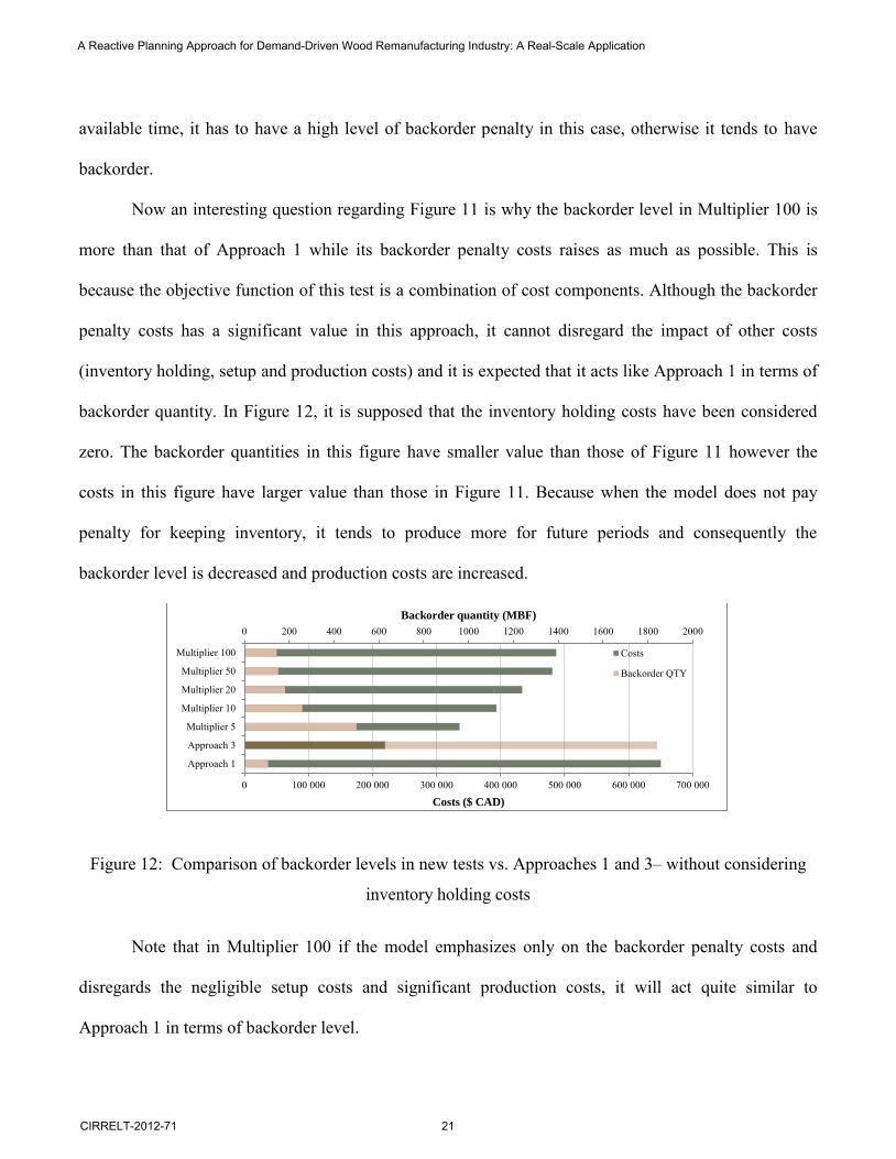
Now an interesting question regarding Figure 11 is why the backorder level in Multiplier 100 is
more than that of Approach 1 while its backorder penalty costs raises as much as possible. This is
because the objective function of this test is a combination of cost components. Although the backorder
penalty costs has a significant value in this approach, it cannot disregard the impact of other costs
(inventory holding, setup and production costs) and it is expected that it acts like Approach 1 in terms of
backorder quantity. In Figure 12, it is supposed that the inventory holding costs have been considered
zero. The backorder quantities in this figure have smaller value than those of Figure 11 however the
costs in this figure have larger value than those in Figure 11. Because when the model does not pay
penalty for keeping inventory, it tends to produce more for future periods and consequently the
backorder level is decreased and production costs are increased.
Figure 12: Comparison of backorder levels in new tests vs. Approaches 1 and 3– without considering
inventory holding costs
Note that in Multiplier 100 if the model emphasizes only on the backorder penalty costs and
disregards the negligible setup costs and significant production costs, it will act quite similar to
Approach 1 in terms of backorder level.
0 200 400 600 800 1000 1200 1400 1600 1800 2000
0 100 000 200 000 300 000 400 000 500 000 600 000 700 000
Approach 1
Approach 3
Multiplier 5
Multiplier 10
Multiplier 20
Multiplier 50
Multiplier 100
Backorder quantity (MBF)
Costs ($ CAD)
Costs
Backorder QTY
A Reactive Planning Approach for Demand-Driven Wood Remanufacturing Industry: A Real-Scale Application
CIRRELT-2012-71 21
6. Conclusion and future directions
This paper described the production planning problems and models for a real-scale wood
remanufacturing unit in the North American forest industry. This unit, like many other production units,
faced with demand fluctuations and absence of an effective plan for handling these fluctuations.
We applied an approach for revising a plan at regular intervals in order to respond to demand
fluctuations. The simulation experiments demonstrated the advantage, in term of responding to
uncertainties by the complete re-planning strategy through the periodic policy. First, the effectiveness of
different approaches was examined in the reactive planning strategy. We observed that the performance
of suggested strategy was sensitive to model objective functions. According to performance of
backorder level and costs value and also predictions for the future, among different proposed planning
approaches, Approach 4 had good results. On the other side, Approach 1 with minimum level of
backorder had the best results in terms of backorder level, although it had high level of costs. Second,
we noted that re-planning frequency had significant impact on the performance of planning methods.
The configurations with the low re-planning period length upon high planning time window performed
better than the other ones. This observation also was held in all approaches.
The approach proposed in the present paper can be extended in many ways. We intend that some
of the assumptions will be consistent with reality, for instance variable setup time. These new constraints
will certainly increase the backorder level. Then an inventory policy will be developed to improve the
efficiency of the reactive planning strategy in a co-production system.
Acknowledgement
This work was supported by Natural Sciences and Engineering Research Council of Canada (NSERC) strategic
network on value chain optimization.
A Reactive Planning Approach for Demand-Driven Wood Remanufacturing Industry: A Real-Scale Application
22 CIRRELT-2012-71
References
Aytug, H., Lawley, M.A., Mckay, K., Mohan, S. & Uzsoy, R., 2005. Executing production schedules in
the face of uncertainties: A review and some future directions. European Journal of Operational
Research, 161 (1), 86-110.
Cowling, P. & Johansson, M., 2002. Using real time information for effective dynamic scheduling.
European Journal of Operational Research, 139 (2), 230-244.
Duenas, A. & Petrovic, D., 2008. An approach to predictive-reactive scheduling of parallel machines
subject to disruptions. Annals of Operations Research, 159 (1), 65-82.
Frantzen, M., Ng, A.H.C. & Moore, P., 2011. A simulation-based scheduling system for real-time
optimization and decision making support. Robotics and Computer-Integrated Manufacturing,
27 (4), 696-705.
Gholami, M. & Zandieh, M., 2009. Integrating simulation and genetic algorithm to schedule a dynamic
flexible job shop. Journal of Intelligent Manufacturing, 20 (4), 481-498.
Gupta, A. & Maranas, C.D., 2003. Managing demand uncertainty in supply chain planning. Computers
& Chemical Engineering, 27 (8-9), 1219-1227.
Itami, R.M., Zell, D., Grigel, F. & Gimblett, H.R., 2005. Generating confidence intervals for spatial
simulations: Determining the number of replications for spatial terminating simulations., 141-148.
Li, Z.K. & Ierapetritou, M., 2008. Process scheduling under uncertainty: Review and challenges.
Computers & Chemical Engineering, 32 (4-5), 715-727.
Lou, P., Liu, Q., Zhou, Z., Wang, H. & Sun, S., 2012. Multi-agent-based proactive–reactive scheduling
for a job shop. The International Journal of Advanced Manufacturing Technology, 59 (1), 311-
324.
Ouelhadj, D. & Petrovic, S., 2009. A survey of dynamic scheduling in manufacturing systems. Journal
of Scheduling, 12 (4), 417-431.
Sabuncuoglu, I. & Bayiz, M., 2000. Analysis of reactive scheduling problems in a job shop
environment. European Journal of Operational Research, 126 (3), 567-586.
Sun, J. & Xue, D., 2001. A dynamic reactive scheduling mechanism for responding to changes of
production orders and manufacturing resources. Computers in industry, 46 (2), 189-207.
Vieira, G.E., Herrmann, J.W. & Lin, E., 2003. Rescheduling manufacturing systems: A framework of
strategies, policies, and methods. Journal of Scheduling, 6 (1), 39-62.
Wan, Y.W., 1995. Which is better, off-line or real-time scheduling. International Journal of Production
Research, 33 (7), 2053-2059.
A Reactive Planning Approach for Demand-Driven Wood Remanufacturing Industry: A Real-Scale Application
CIRRELT-2012-71 23


![Aalborg Universitet A Data-Driven Stochastic Reactive Power … · leads to the development of the dynamic reactive power opti-mization (DRPO) model [1-3]. This model is actually](https://cdn.vdocument.in/doc/165x107/5ec98c17677e3c7a135930f0/aalborg-universitet-a-data-driven-stochastic-reactive-power-leads-to-the-development.jpg)
