A Semi-Parametric Bayesian Approach to the Instrumental Variable Problem
by
Tim Conley Chris Hansen
Rob McCulloch Peter E. Rossi
Graduate School of Business
University of Chicago
June 2006 Revised, December 2007
Keywords: instrumental variables, semi-parametric Bayesian inference, Dirichlet process priors JEL classification: C11, C14, C3
Abstract We develop a Bayesian semi-parametric approach to the instrumental variable problem. We assume linear structural and reduced form equations, but model the error distributions non-parametrically. A Dirichlet process prior is used for the joint distribution of structural and instrumental variable equations errors. Our implementation of the Dirichlet process prior uses a normal distribution as a base model. It can therefore be interpreted as modeling the unknown joint distribution with a mixture of normal distributions with a variable number of mixture components. We demonstrate that this procedure is both feasible and sensible using actual and simulated data. Sampling experiments compare inferences from the non-parametric Bayesian procedure with those based on procedures from the recent literature on weak instrument asymptotics. When errors are non-normal, our procedure is more efficient than standard Bayesian or classical methods.
1
1. Introduction
Instrumental variables (IV) methods are fundamental in applied economic research.
However, because IV methods exploit only that portion of the variation in the endogenous
variable induced by shifting the instrumental variable, inference tends to be imprecise. This
problem is exacerbated when the instruments are only weakly related to the endogenous
variables and induce only small amounts of variation. The recent econometrics literature has
included numerous papers which present potential improvements to the usual asymptotic
approaches to obtaining estimates and performing inference in IV models.1
We present a Bayesian instrumental variables approach that allows nonparametric
estimation of the distribution of error terms in a set of simultaneous equations. Linear
structural and reduced form equations are assumed. Thus, our Bayesian IV procedures is
properly termed, semi-parametric. Bayesian methods are directly motivated by the fact that
researchers are quite likely to have informative prior views about potential values of
treatment parameters, placing a premium upon methods allowing the use of such
information in estimation. Weak instrument problems are inherently small sample problems
in that there is little information available in the data to identify the parameter of interest. As
Bayesian methods are inherently small sample, they are a coherent choice. Even in the
absence of a direct motivation for using Bayesian methods, we provide evidence that
Bayesian interval estimators perform well compared to available frequentist estimators,
under frequentist performance criteria.
The Bayesian semi-parametric approach attempts to uncover and exploit structure in
the data. For example, if the errors are truly non-normal, the version of our model with
varying error distribution parameters would fit this distribution and may provide efficiency

2
gains from this information. In contrast, traditional instrumental variable methods are
designed to be robust to the error distribution and, therefore, may be less efficient. In the
case of normal or nearly normal errors, our procedure should have a small efficiency loss.
Our nonparametric method for estimating error term distributions can be interpreted
as a type of mixture model. Rather than choosing a fixed number of base distributions to be
mixed, we specify a Dirichlet Process (DP) prior that allows the number of mixture
components to be determined by both the prior and the data. The alternative of using a
pre-specified number of mixture components requires some sort of auxiliary computations
such as Bayes Factors to select the number of components. In our approach, this is
unnecessary as the Bayes Factor computations are undertaken as part of the MCMC method.
There is also a sense that the DP prior is a very general approach which allows model
parameters to vary from observation to observation. A posteriori observations which could
reasonably correspond to the same error distribution parameter are grouped together. This
means that the DP approach handles very general forms of heterogeneity in the error
distributions.
Our implementation of the normal base model and conjugate prior is entirely
vectorized except for one loop in a sub Gibbs Sampler for drawing the parameters governed
by the DP prior which is currently implemented in C. This makes DP calculations feasible
even in a sampling experiment and for the sample sizes often encountered in applied cross-
sectional work. Computational issues are discussed in appendix A.
We conduct an extensive Monte Carlo evaluation of our proposed method and
compare it to a variety of classical approaches to estimation and inference in IV models. We
examine estimators’ finite sample performance over a range of instrument strength and
1 See for example, Stock, Wright, and Yogo (2002) or Andrews, Stock, and Moreira (2006) for excellent

3
under departures from normality. The semi-parametric Bayes estimators have smaller
RMSE than standard classical estimators. In comparison to Bayesian methods that assume
normal errors, the non-parametric Bayes method has identical RMSE for normal errors and
much smaller RMSE for log-normal errors. For both weak and strong instruments, our
procedure produces credibility regions that are much smaller than competing classical
procedures, particularly in the case of non-normal errors. For the weak instrument cases,
our coverage rates are four to twelve percent below the nominal coverage rate of 95 per
cent. Recent methods from the weak instrument classical literature produce intervals with
coverage rates that are close to nominal levels but at the cost of producing extremely large
intervals. For log-normal errors, we find these methods produce infinite intervals more than
40 per cent of the time.
The remainder of this paper is organized as follows. Section 2 presents the main
model and the essence of our computation algorithm. Section 3 discusses choices of priors.
In Section 4, we present two illustrative empirical example applications of our method.
Section 5 presents results from sampling experiments which compare the inference and
estimation properties of our proposed method to alternatives in the econometrics literature.
Section 6 provide timing and autocorrelation information on the Gibbs sampler as well as
the results of the Geweke (2004) tests for the validity of the sampler and code. Appendices
detail the computational strategy and provide specifics of the alternative classical inference
procedures considered in the paper.
overviews of this literature.

4
2. Model and MCMC
In this section, we present a version of the instrumental variable problem and explain how to
conduct Bayesian inference for it. Our focus will be on models in which the distribution of
error terms is not restricted to any specific parametric family. We also indicate how this
same approach can be used in models with unknown regression or mean functions.
2.1 The Linear Model
Consider the case with one linear structural equation and one “first-stage” or
reduced form equation.
(2.1) '
1,'
2,
i i i
i i i i
x z
y x w
δ ε
β γ ε
= +
= + +
y is the outcome of interest, x is a right hand side endogenous variable, w is a set of
exogenous covariates, and z is a set of instrumental variables that includes w. The
generalization of (2.1) to more than one right hand side endogenous variables is obvious. If
ε1 and ε2 are dependent, then the treatment parameter, β, is identified by the variation
from the variables in z, which are excluded from the structural equation and are commonly
termed “instrumental variables.” Classical instrumental variables estimators such as two
stage least squares do not make any specific assumptions regarding the distribution of the
error terms in (2.1). In contrast, the Bayesian treatment of this model has relied on the
assumption that the error terms are bivariate normal (c.f. Chao and Phillips (1998), Geweke
(1996), Kleibergen and Van Dijk (1998), Kleibergen and Zivot (2003), Rossi, Allenby and
McCulloch(2005), and Hoogerheide, Kleibergen, and Van Dijk (2007)).2
2 An exception is Zellner (1998) whose BMOM procedure does not use a normal or any other specific parametric family of distributions of the errors.

5
(2.2) ( )1,
2,~ ,i
ii
Nε
ε με
⎛ ⎞= Σ⎜ ⎟
⎝ ⎠
For reasons that will become apparent later, we will include the intercepts in the error terms
by allowing them to have non-zero mean, μ .
Most researchers regard the assumption of normality as only an approximation to the
true error distribution. Some methods of inference such as those based on TSLS and the
more recent weak and many instruments literature do not make any explicit distributional
assumptions. In addition to outliers, some forms of conditional heterogeneity and mis-
specification of the functional forms of the regression functions can produce non-normal
error terms. For these reasons, we develop a Bayesian procedure that uses a flexible error
distribution that can be given a non-parametric interpretation.
Our approach builds on the normal based model but allows for separate error
distribution parameters, ( ),i i iθ μ= Σ for every observation3. As discussed below, this
affords a great deal of flexibility in the error distribution. However, as a practical matter
some sort of structure must be imposed on these set of parameters, otherwise we will face a
problem of parameter proliferation. One solution to this problem is to use a prior over the
collection, { }iθ , which creates dependencies. In our approach, we use a prior that clusters
together “similar” observations into groups and use *I to denote the number of these
groups. Each of the *I groups has its own unique value of θ. The value of *I will be
random as well, allowing for a truly non-parametric method in which the number of clusters
can increase with the sample size. In any fixed size sample, our full Bayesian implementation
will introduce additional parameters only if necessary, avoiding the problem of over-fitting.
6
With a normal base distribution, the resulting predictive distribution of the error
terms (see section 2.4 for details) will involve a mixture of normal distributions where the
number and shape of the normal components is influenced by both the prior and the data.
A mixture of normals can provide a very flexible approximation device. Thus, our
procedure enjoys much of the flexibility of a finite mixture of normals without requiring
additional computations/procedures to determine the number of components and impose
penalties for over-fitting. It should be noted that a sensible prior is required for any
procedure that relies explicitly or implicitly (as ours does) on Bayes Factor computations.
In our procedure, observations with large errors can be grouped separately from
observations with small errors. The coarseness of this clustering is dependent on the
information content of the data and the prior settings. In principle, this allows for a general
form of heteroskedasticity with different variances for each observation. 2.2 Flexible Specifications through a Hierarchical Model with a Dirichlet Process Prior
Our approach to building a flexible model is to allow for a subset of the parameters to vary
from observation to observation. We can partition the full set of parameters into a part that
is fixed, η , and one that varies from observation to observation, θ . For example, we could
assign ( )η β δ γ= , , and ( )θ μ= Σ, as suggested above. The problem becomes how to put
a flexible prior on the collection, { }θ =1Nii . The standard hierarchical approach is to assume
that each θi is iid ( )λ0G where 0G is some parametric family of distributions with
hyperparameters, λ . Frequently, a prior is put on λ and this has the effect of inducing
dependencies between the iθ .
3 Our approach is closest to that of Escobar and West (1995) who consider the problem of Bayesian density estimation for direct observation of univariate data using mixtures of univariate normals.

7
A more flexible approach is to specify a DP prior for G instead.
(2.3) ( )0
~~ ,
i iid GG DP Gθ
α
( )0,DP Gα denotes the DP with concentration parameter α and base distribution 0G . G
is a random distribution such that with probability one G is discrete. This means that
different iθ may correspond to the same atom of G and hence be the same. This is a form
of dependency in the prior achieved by clustering together some of the iθ . It should be
noted that while each draw of G is discrete this does not mean that the joint prior
distribution on { }θ =1Nii is discrete once G has been margined out. This distribution is called
a mixture of Dirichlet Processes and is shown in Antoniak (1974) to have continuous
support. It is worth noting that the marginal distribution of any iθ is oG . The sole purpose
of the DP prior is to introduce dependencies in the collection, { }θ =1Nii .
A useful way to gain some intuition as to the DP prior is to consider the “stick-
breaking” representation of this prior (Sethuraman (1994)). Each draw from G is a discrete
distribution. The support or “atoms” of this distribution are iid draws from oG . The
probability weights are obtained as ( )11 1k
k k jjπ ω ω−== −∏ , with 0 0ω = and
( )~ 1,k Betaω α . Thus, a draw G can be represented as 1 kkkG Iθπ∞== ∑ , where Iθ is a
point mass at atom θ , the kθ are i.i.d. draws from oG .
The distribution of the atom weights depends only on α. We obtain the π weights
by starting with the full mass one and repeatedly taking bites of size kω out of the remaining
weight. If α is big we will take small bites so that the mass will be spread out over a large
number of atoms. In this case, G will be a discrete approximation of oG so that the draws
of G will be close to oG and the { }iθ will essentially be i.i.d draws from oG . If α is small,
we will take big bites and a draw of G will put large weight on a few random draws from

8
oG . In this case, the { }iθ contain only a few unique values. The number of unique values is
random with values between one and N being possible.
Suppressing the fixed parameters η , we can write our basic model in hierarchical
form as the set of the following conditional distributions:
(2.4) ( )
{ }( )
0~ ,
, ,i
i i i i
G DP G
G
x y z
α
θ
θ
In the posterior distribution for this model, the prior and the information in the data
combine to identify groups of observations which could reasonably share the same θ. In
section 3, we consider priors on the DP concentration parameter α and the selection of the
base prior distribution, oG . Roughly these two priors delineate the number and type of
atoms generated by the DP prior.
2.3 MCMC Algorithms
The fixed parameter, linear model in (2.1) and (2.2) has a Gibbs Sampler as defined in Rossi
Allenby, and McCulloch (2005) (see also Geweke (1996)) consisting of the following
conditional posterior distributions:
(2.5) , , , , , , ,y x Z Wβ γ δ μ Σ
(2.6) , , , , , , ,y x Z Wδ β γ μ Σ
(2.7) , , , , , , ,y x Z Wμ β γ δΣ
where , , ,y x Z W denote vectors and arrays formed by stacking the observations. The key
insight needed to draw from (2.5) is that, given δ, we “observe” 1ε and we can compute
the conditional distribution of y given x, Z, W and 1ε . The parameters of this conditional

9
distribution are “known” and we simply standardize to obtain a draw from a Bayes
regression with N(0,1) errors. The draw in (2.6) is effected by transforming to the reduced
form which is still linear in δ (given β). This exploits the linearity (in x) of the structural
equation. Again, we standardize the reduced form equations and stack them to obtain a
draw from a Bayes regression with N(0,1) errors. The last draw (2.7) simply uses standard
Bayesian multivariate normal theory using the errors as “data.”
If some subset of the parameters is allowed to vary from observation to observation
with a DP prior, we then must add a draw of these varying parameters to this basic set-up.
For example, if we define ( ),i i iθ μ= Σ , then the Gibbs Sampler becomes
(2.8) β γ α δ Θ, , , , , , ,y x Z W
(2.9) δ α β γ Θ, , , , , , ,y x Z W
(2.10) α β γ δΘ , , , , , , ,y x Z W
(2.11) , , , , , , ,y x Z Wα β γ δΘ
{ }iθΘ = . The draws in (2.8) and (2.9) are the same as for the fixed parameter case except
that the regression equations must be standardized to have zero mean errors and unit
variance. Since Θ contains only *I unique elements, we can group observations by unique
iθ value and standardize each with different error means and covariance matrices. This
presents some computing challenges for full vectorization but it is conceptually
straightforward. The draw of Θ in (2.10) is done by a Gibbs sampler which cycles thru each
of the N iθ s (Escobar and West (1998); see appendix A for full details). The input to this
Gibbs Sampler as “data” is the matrix (N x 2) of error terms computed using the last draws
of ( ), ,β δ γ . Each draw of Θ will contain a different number ( )N≤ of unique values.

10
The draw of α is a straightforward univariate draw (see appendix A for details). Thus, this
model can be interpreted as a linear structural equations model with errors following a
mixture of normals with a random number of components which are determined by the data
and prior information.
2.4 Bayesian Density Estimation
One useful by-product of our DP MCMC algorithm is a very simple way of obtaining an
error density estimate directly from the MCMC draws without significant additional
computations. In the empirical examples in section 4, we will display some of these density
estimates in an effort to document departures from normality. The Bayesian analogue of a
density estimate is the predictive distribution of the random variables for which a density
estimate is required. In our case, we are interested in the predictive distribution of the error
terms. This can be written as follows:
(2.12) ( ) ( ) ( )1 1 1 1N N N Np Data p p Data dε ε θ θ+ + + += Θ∫
We can obtain draws from 1N Dataθ + using (2.13) ( ) ( ) ( )1 1N Np Data p p Data dθ θ+ += Θ Θ Θ∫
Since each draw of Θ has *I N< unique values, and the base model, ( )p ε θ , is a normal
distribution, we can interpret the predictive distribution or density estimation problem as
involving a mixture of normals. This mixture involves a random number of components.
To implement this, we simply draw from 1Nθ + Θ for each draw of Θ returned by our
MCMC procedure (see appendix A for the details of this draw). Denote these draws by
1rNθ + , 1, ,r R= K . The Bayesian density “estimate” is simply the MCMC estimate of the
posterior mean of the density ordinate.
11
(2.14) ( ) ( )11
1ˆR
rN
rp
Rε ϕ ε θ +
== ∑
where ( )ϕ is the bivariate normal density function.
2.5 Generalizations of the Linear Model
The model and MCMC algorithm considered here can easily be extended. We have
emphasized the use of the DP prior for the parameters of the error terms but we could easily
put the same prior on the regression coefficients and allow these to vary from observation to
observation as in
(2.15) 'i i i i i iy x wβ γ ε= + +
This is a general method for approximating an unknown mean function. The regression
coefficients will be grouped together and can assume different values in different regions of
the regressor space (Geweke and Keane (2007) consider a mixture of normals approach with
a fixed number of components for regression coefficients). In addition, a model of the
form in (2.15) would allow for conditional heteroskedasticity. Implementation of this
approach would require separate a DP prior for the coefficients. Some of the computations
in the Gibbs sampler for the DP parameters would have to change but our modular
computing method would easily allow one to plug in just a few sub-routines. Moreover, the
conjugate prior computations required would be less elaborate than for the DP model for
multivariate normal error terms. An interesting special case of (2.15) would be the model
with heterogenous treatment effects.
(2.16) 'i i i i iy x wβ γ ε= + +
Here interest would focus on identifying subsets of the observations with different effects of
x on y. The computational algorithms for (2.15) or (2.16) are straightforward extensions of

12
what we have already implemented. The real work would be in the assessment of reasonable
priors and in methods for interpreting the results.

13
3. Hyperparameters and Prior
In the Bayesian literature on structural equations models, there has been an emphasis on
developing various reference priors. For example, Chao and Philips and Kleiberger and
Zivot consider a Jeffreys’ prior which they show provides a posterior with similarities to the
sampling distribution of the LIML estimator. Hoogerheide, Kleibergen, and Van Dijk
extend these results to allow for the incorporation of additional sources of prior information.
It should be noted that these reference priors depend on the information matrix of the
normal error likelihood. In this sense, this Bayesian literature is highly dependent on the
normality assumption both for the form of the likelihood and the prior. Since we do not
employ a normal likelihood, these reference priors are not applicable. In general, the
Dirichlet Process prior is a proper prior and there are no improper reference priors that can
be used with this approach.
We develop a prior for the model (2.1)- (2.2) and associated Gibbs sampler (2.8)-(2.11).
Priors are chosen to enable us to capture reasonable prior information and for convenience
in making the draws. The choices include the family 0G and associated parameters λ , the
prior on ( ), ,β δ γ , and the prior on the DP parameter α. We will let ( ),β γ , δ and α be a
priori independent. In some of the previous Bayesian literature, priors have been used that
make β and δ a priori dependent. Again, this comes from an appeal to the form of the
likelihood. As δ gets small, the likelihood over β spreads out, approaching the limiting case
in which β is not identified. There is no necessary reason why the prior should take the
form of the likelihood. More importantly, it is the prior on the covariance structure of the
error terms that really governs the behavior of the posterior of β in the weak instruments
case (see Rossi et al (2007), chapter 7).
14
Our approach will be to put a prior on α which will admit a reasonable a priori
distribution of the number of unique iθ values. We will choose λ rather than put a prior on
this quantity. By inspecting properties of the 0G prior, direct assessment of λ is possible if
we standardize our data. Although the use of standardization does make our prior data
dependent, we feel that our choices result in a prior which is relatively uninformative without
being unreasonable in the sense of putting prior probabilities on absurd values of iθ . We
note that our approach is very different from an empirical Bayes approach in which λ is
chosen to maximize the probability of the observed data. We also note that our focus is on
inference about the structural parameters and not the density of the error terms in (2.1).
Density estimation involves inference about the process by which iθ values are obtained. In
that case, a prior on λ would allow for inference about this process in the sense that we
would make posterior inferences about λ and this would, in turn, affect the predictive
distribution of the error terms which is the Bayesian analogue of density estimation.
In our model, β is a single parameter of key interest. β summarizes the effect on y
caused by an intervention through x. It is plausible that prior information may exist for this
parameter. The other prior choices are both more complex and less interesting to the
investigator. Our hope is to make simple, reasonable choices that are not overly influential.
Of course, some researchers view the need to make these prior choices as an additional cost
of using the Bayesian approach. The Bayesian views this as an important opportunity to
inject information which may be especially helpful in cases with weak instruments, for
example. We note that some of the Bayesian procedures in the literature put priors on the
reduced form parameters rather than directly on the structural parameters. Subjective prior
information is available for the structural parameter but rarely for the reduced form
15
regression coefficients. Thus, those procedures are best viewed as in the spirit of reference
priors designed for the situation where the investigator has little or no information about the
structural parameters or is reluctant to use this information. Hoogerheide, Kleibergen and
Van Dijk specify an informative prior on the reduced form coefficients but require
information on the prior mean of the structural parameter as part of the prior assessment
procedure.
It is convenient to specify normal priors, ( )~ ,N Vδ δδ μ and ( ) ( ), ~ ,N Vβγ βγβ γ μ
as the MCMC draws are normal. In many applications, this could be simplified further by
assuming that β and γ are a priori independent. Specifying a univariate normal prior for β
is appealing as we would only have to think about reasonable values of y xΔ Δ .
The choice of priors for the DP is more complicated. α governs the number of
clusters of observation-specific parameters and 0G influences the values of the unique
values of parameters corresponding to each cluster.
3.1 Choice of 0G and λ
Recall that in making the draw (2.10), we may act as if we observe the errors iε , where
( )~ ,i i iNε μ Σ and we let ( ),i i iθ μ= Σ .
In order to make this draw using the method in Escobar and West (1998), we need to
be able to compute ( ) ( )ε θ θ λ∫ 0p dG for a single ε and draw from the posterior of a
single θ given prior ( )0G λ and an observed set of i.i.d ε assumed to correspond to that
single θ. These requirements make the choice of a (conditionally) conjugate prior extremely
convenient as in this case both of these operations are relatively straightforward. The form
of the conjugate prior is,
(3.1) ( ) ( )1~ , , ~ ,IW V N aυ μ μ −Σ Σ Σ
16
where IW denotes the inverted-Wishart distribution parameterized so that [ ]1 1E Vυ− −Σ = .
Given this choice, ( ), , ,V aλ υ μ= . For the Bayesian procedure based on normal errors,
we use the same natural conjugate prior for θ and the same values of λ.
Now our problem is to choose λ such that draws from ( )0G λ are reasonable values
for iθ . We start by assuming that we have translated and rescaled x and y so that both are in
the range [ ],c c− with high probability. In practice, a convenient way to do this is to apply
the transformation which standardizes the observed iy and ix to have mean zero and
sample standard deviation one and use 2c = . We shall follow this procedure in our
examples, but note that the transformation and c could reasonably be chosen from prior
information.
Given our standardization, 0μ = is an obvious choice and V vI= where I is the 2 2×
identity matrix is a reasonable choice. The prior on μ governs the location of the atoms and
the prior on Σ influences both the spread of the μ values as well as the shape of each normal
atom. If a large number of atoms are used, it is unlikely to matter much what shapes are a
priori most probable (i.e. whether the atoms are correlated or uncorrelated normals).
However, with small numbers of atoms this may matter. Our assessment procedure allows
for a relatively large (potential) number of atoms. This means that the prior on μ
determines the implied prior of the error distribution. Since we spread our atoms over the
error space evenly in all quadrants, our prior specification weakly favors independence of the
errors. Thus, in the case of data sets with little information, our Bayes estimators will
“shrink” toward the case of no endogeneity.
17
To see this, consider the predictive distribution of the error terms under the Dirichlet
Process prior. Recall that the marginal distribution of iθ is ( )0G λ . Therefore, the
predictive distribution, ( ) ( ) ( )0p p dGε ε θ θ λ= ∫ , is a multivariate student t with a
diagonal location matrix, V. This distribution has zero correlation between the two errors
(there is dependence but only in the scale). If we put in a non-diagonal value for V, this
could be changed. The problem, however, is that we rarely have a priori information about
the sign and magnitude of the error dependence. Thus, we think the choice of diagonal V is
a reasonable default choice.
We now have three scalar quantities ( ), ,v aυ to choose. To make these choices we
must think about what kinds of normal distributions are possible for the iε . The largest
errors would occur when δ, β, and γ are zero so that the iε are like the ( ),i ix y . Thus we
need the priors to be spread out enough for μ to cover possible ( ),i ix y and Σ to explain
the variation of ( ),i ix y in the case where all observations share the same θ.
To make the choice of ( ), ,v aυ more intuitive, consider the implied marginals for
1 11σ σ= and 1μ . We assess intervals for these marginals and then compute the
corresponding values for ( ), ,v aυ . Define the intervals as
(3.2) [ ] [ ] [ ]σ σ κ μ κ< = < = − < < = −1 1 1 2 3 1 3/ 2, 1Pr c Pr c Pr c c
Given κ , choosing ( ), ,v aυ is equivalent to choosing 1c , 2c , and 3c . For example, if we
use .2κ = , 1 .25c = , 2 3.25c = , and 3 10c = , this gives 2.004υ = , .17v = , and .016a = .
These values we term our “default” prior and are used in our sampling experiments and our
empirical examples (see sections 4 and 5). While these choices may seem to be “too” spread
out given our choice of standardization, the goal is to be as diffuse as possible without
allowing absurd choices. If the resulting posteriors are very sensitive to these prior choices,
18
then we would have a problem. However, we will see in our examples that this does not
seem to be the case. The marginal distributions required to evaluate (3.2) are
(3.3) ( )211 1 1~ , ~ 1v v a tυ υσ χ μ υ− −−
3.2 Prior on α
What is a reasonable value for α ? In section 2, we saw that α contributes to G through the
weights, kπ . However, since the corresponding atoms are i.i.d ( )0G λ , the weights are not
interpretable in a simple manner. As with our choice of λ, we will use a prior marginal to
guide our choice of α. Our goal in using the DP model is to group observations so that
observations within the same group share the same θ. Given N, the number of observations,
we will consider the prior marginal on the number of groups, or equivalently, the number of
unique θ values obtained by first drawing ( )~ ,G DP α λ and then N iid ~ Gθ . Let *I
denote the number of unique θ (given N). Recall that when α is large, the π weights will
be spread out so that *I will tend to be large. When α is small, only a few π will be large
so *I will tend to be small.
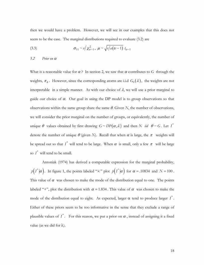
Antoniak (1974) has derived a computable expression for the marginal probability,
( )*p I α . In figure 1, the points labeled “× ” plot ( )*p I α for .10834α = and 100N = .
This value of α was chosen to make the mode of the distribution equal to one. The points
labeled “+”, plot the distribution with 1.834α = . This value of α was chosen to make the
mode of the distribution equal to eight. As expected, larger α tend to produce larger *I .
Either of these priors seem to be too informative in the sense that they exclude a range of
plausible values of *I . For this reason, we put a prior on α , instead of assigning it a fixed
value (as we did for λ).

19
We develop a new prior for α by first choosing a small value α so that the
corresponding mode of ( )*p I α is small, and a large value α , so that the corresponding
mode of ( )*p I α is large. We then distribute our prior probability for α on a grid of
points between α and α according to,
(3.4) ( ) 1pωα αα
α α−⎛ ⎞∝ −⎜ ⎟−⎝ ⎠
.
The points labelled “g” in figure 1 show the marginal prior distribution of *I given
100N = and the choices .10834α = and 1.834α = , and .8ω = . That is, for each value
of i , we compute ( ) ( )*p p I iα α=∑ . This marginal is nicely spread out between the
other two distributions in the figure corresponding to the extreme choices α and α which
have *I modes of 1 and 8, respectively. These prior settings are used in the sampling
experiments reported in section 5 and our first empirical example in section 4.1. For our
second empirical example in section 4.2, we modify these prior settings to allow an increased
[ ,α α ] range corresponding to *I modes of 1 to 30.
This prior formulation gives us a simple way to think about α in terms of our
motivation for using the DP prior: groups of observations. A drawback is that it depends on
N, but given the meaning of the parameter this seems reasonable. Putting a prior on α rather
than just fixing it, makes it easier for the data to guide us in determining the number of
groups. Appendix A gives details on the posterior draw of α in (2.11).
20
4. Empirical Examples
In this section, we consider two empirical examples of the application of our methods. We
include examples with small and moderately large numbers of observations.
4.1 Acemoglu
The first example is due to Acemoglu, Johnson, and Robinson (2001) who consider the
relationship between GDP per capita and a measure of the risk of expropriation. To solve
the endogeneity problem, European settler mortality is used as an instrument. In former
colonies with high settler mortality, Acemoglu and co-authors argue that Europeans could
not settle and, therefore, set up more extractive institutions. We consider a specification
which is a structural equation with log GDP related to Average Protection Against Ex-
propriation Risk (APER), latitude and continent dummies4 along with a first stage regression
of APER on log European Settler Mortality and the same covariates as in the structural
equation. The incremental R-squared from the addition of the instrument is .02 with a
partial F statistic of 2.25 on 1 and 61 degrees of freedom. The least squares coefficient on
APER is .42 while the TSLS coefficient is 1.41 in this specification. The conventional
asymptotics yield at 95 per cent C.I. of (-.015, 2.97) with N=64. The CLR procedure
provides a disjoint and infinite C.I. of ( )−∞ − ∞( , 2.35) .66,∪ , suggesting that conventional
asymptotics are not useful here due to a weak instrument problem.
Both the conventional and CLR-based confidence intervals extend over a very wide
range of values. This motivates an interest in methods with greater efficiency. It is also
possible to argue that a non-parametric method would overfit this small dataset so this
example will stress test our Bayesian method with a Dirichlet Prior. Figure 2 shows the
4 The continent dummies used were Africa, Asia and “Neo.” Neo includes the former British colonies of Australia, Canada, New Zealand and the United States.

21
posterior distribution using normal errors (top panel) with Dirichlet Prior. We use the
“default” prior settings for λ and values of ,α α corresponding to *I modes of 1 and 8
respectively. The Bayes 95 per cent credibility interval5 is drawn on the horizontal axis with
light brackets. The interval for the normal error model is (.13, 1.68) and the interval for the
DP Prior model is (.05,1.2). The inferences from a Bayesian procedure with normal errors
are not too different from conventional TSLS estimates. However, the interval derived from
the Bayes-DP model is considerably shorter and is located nearer the least squares estimates.
Figure 3 shows the fitted density of the errors constructed as the Posterior Mean of
the error density. This density displays some aspects of non-normality with diamond-shaped
contours.
4.2 Card Example
Card (1995) considers the time honored question of the returns to education, exploiting
geographic proximity to two and four year colleges as an instrument. He argues that
proximity to colleges is a source of exogeneous changes in the cost of obtaining an
education which will cause some to pursue a college education when they might not
otherwise do so. The basic structural equation relates log of wage to education (years),
experience, experience-squared, black dummy variable, and indicator for residing in a
standard metropolitan statistical area, South indicator variable and various regional
indicators. The first stage is a regression of education on two indicators for proximity to
two and four year colleges and the same covariates as in the structural equation. The
incremental R-squared from the addition of the instruments to the first state is .0052 with
corresponding F of 7.89 on 2 and 2993 degrees of freedom. OLS estimates of the return to
5 These credibility intervals are the intervals between .025 to .975 quantiles of the relevant posterior

22
education are around .07 while the TSLS estimates are much higher, around .157 with a
standard error of .052, N=3010. The LIML estimate is .164 with a standard error of .055.
To our view, these returns of 14 per cent per year of education seem high. However, even
with more than three thousand observations, the confidence interval for the returns on
education is very large.
Figure 4 shows the posterior distributions assuming normal errors and using the DP
prior. The 95 per cent posterior credibility regions are denoted by light brackets. For the
normal error case, the interval is (.058, .34) while it is (.031, .17) for the DP Prior model. We
use the “default” prior settings for λ and values of ,α α corresponding to *I modes of 1
and 30 respectively. As in the Acemoglu data, the normality assumption makes a difference.
With the DP prior, the posterior distribution is much tighter and centered on a lower rate of
return to education. There is less “endogeneity” bias if one allows for a more flexible error
distribution. Figure 5 shows the fitted density from the DP prior procedure (bottom panel)
as well as the predictive density of the errors from a Bayesian procedure that assumes the
error terms are normal (top panel). There are marked differences between these densities.
The normal error model concludes that there is substantial negative correlation in the errors,
while the Bayesian non-parametric model yields a distribution with pronounced skewness
and non-elliptical contours, showing little dependence. It is possible that outlying
observations are driving this result. In any event, the assumption of normality has
substantial implications for the inference about the structural quantity.
These examples illustrate that our Bayesian procedures give reasonable results for a
wide range of sample sizes, and it matters whether or not one specifies a normal distribution
of the error terms. Moreover, it appears that the Bayesian non-parametric model is capable
distribution, in general they differ from highest posterior density intervals.

23
of discovering and exploiting structure in the data, resulting in tighter posterior distributions.
However, this evidence is far from conclusive. For this reason, we consider sampling
experiments in section 5.
24
5. Simulation Studies
The Bayesian semi-parametric procedure outlined in sections 2 and 3 above can be evaluated
by comparison with other Bayesian procedures based on normally distributed equation
errors or by comparison with classical procedures. Comparison with a Bayesian procedure
based on normal errors is straightforward as both procedures are in the same inference
framework. Comparison with classical procedures is somewhat more complicated as
classical methods often draw a distinction between what is termed an “estimation problem”
and an “inference problem.” A variety of k-class estimation procedures have been proposed
for the linear structural equations problem, but the recent classical literature has focused on
improved methods of inference. Inference is often viewed as synonymous with the
construction of confidence intervals with correct coverage probabilities. In this section, we
discuss simulation experiments designed to compare the sampling properties of our Bayesian
semi-parametric procedure with those of alternative Bayes and classical procedures.
5.1 Experimental Design
We consider the model of section 2.1 which is a linear structural equation with one
endogeneous right hand side variable. The simplicity of this case will allow us to explore the
parameter space thoroughly and focus on the effects of departures from normality which we
regard as our key contribution. Moreover, this model is empirically relevant. A survey
(Chernozhukov and Hansen (2005)) of the leading journals in economics (QJE/AER/JPE)
in the period 1996-2004 produced 129 articles using linear structural equations models of
which 89 had only one endogenous right hand side variable. It appears, therefore, that the
canonical use of instrumental variables methods is to allay concerns about endogeneity in
regression models with a small number of potentially endogeneous right hand side variables.
The model considered in our simulation experiments is given below:

25
(5.1) ( ) 1'x z ιδ ε= +
(5.2) 2y xβ ε= +
ι is a vector of k ones. Throughout we assume that 1β = . Since the classical literature
considers both the case of “many” instruments and weak instruments, we will consider the
case in which z is of dimension k = 10. Each element of the z vector is generated as iid
Uniform(0,1) and the z are redrawn for each simulation replicate.
We specify both a normal and log-normal distribution of the error terms in (5.1).
(5.3) ( ) ( )1 1
2 2~ 0, ; ~ ln 0,N or cv v N s
ε εε ε
⎛ ⎞ ⎛ ⎞Σ = Σ⎜ ⎟ ⎜ ⎟
⎝ ⎠ ⎝ ⎠
⎡ ⎤Σ = ⎢ ⎥
⎣ ⎦
1 .6.6 1
, s = .6 and c is taken so that the interquartile range of log-normal variables is
the same as the normal distribution in the base case. The idea is to create skewed errors
without an excessive number of positive outliers.
The value of δ is chosen to reflect various degrees of strength of instruments from a
“weak” to “strong” settings. In the classical literature, the F statistic from the first stage
regression or the concentration parameter, kF, is used to assess the strength of the
instruments. It is also possible to compute the population R-squared implied by a particular
choice of δ.
(5.4) δ
ρδ σ
=+
212 12
211112
kk
We chose three values of δ : (.5, 1.0, 1.5); hereafter we refer to these values as “weak,”
“moderate,” and “strong.” For the normal distribution case, these correspond to population
R-squared values of (.17, .45, .65). These are the approximate quartiles of the empirical

26
distributions of R-squared found in our literature search. Some may object to our
characterization of .17 with 10 instruments as case of weak instruments. The implied p-
value for the F statistic in the weak instrument case with 10 instruments and 100
observations given the population R-squared is .068.
We use a sample size, N, of 100. For each of 400 replications, we draw z values
(uniform on (0,1)) and then errors from the two error distributions specified in (5.3). We
repeat this process for each of three values of delta, resulting in a sampling experiment with
six cells. Figure 6 provides boxplots of the distribution of R-squared and F over each of the
400 replicates for each of our six cells (note that the box extends from the 2.5 to 97.5
percentiles in these plots). We can see that our weak instrument cells contain a substantial
number of datasets with first-stage R-squares below 10 per cent or concentration parameters
below 10.
For each of our generated data sets, we will compute a Bayesian 95 percent Credibility
Interval and the posterior mean using our semi-parametric procedures. We will compare
these intervals and estimates to standard Bayesian estimates using normal errors, standard k-
class estimators and intervals constructed using standard asymptotics, many instrument
asymptotics and weak instrument asymptotics. The next section briefly describes classical
estimation and inference approaches that are compared to our Bayesian procedure.
5.2 Alternative Classical Estimators and Inference Procedures
For comparison, we report results from a variety of other procedures which have
been suggested for point and interval estimation in IV models. We consider four point
estimators: ordinary least squares (OLS), two stage least squares (TSLS), limited information
maximum likelihood (LIML), and Fuller’s (1977) modification of LIML (F1) to produce an
estimator with moments in finite samples. OLS provides a useful benchmark, and TSLS is
27
the most commonly used estimator in instrumental variables contexts though it may have
undesirable properties when the number of instruments is large or instruments are weak.
LIML and F1 have been suggested as alternatives to 2SLS that may perform better when
instruments are many or weak.
For interval estimation, we use large sample approximations in connection with each
of the point estimators described above and, in addition, consider alternative interval
estimators that are robust to weak/many instruments. We construct interval estimates using
the ‘many instrument’ asymptotic approximation of Bekker (1994) for LIML and F1. This
provides an asymptotic refinement of the typical large sample approximations when there
are over-identifying restrictions (Hansen, Hausman, and Newey (2005)). Finally, we consider
three recently proposed procedures for constructing confidence intervals that are robust to
weak identification by test statistic inversion. Specifically, we invert two score-based statistics
due to Kleibergen (2002, 2005) and the conditional likelihood ratio (CLR) statistic proposed
by Moreira (2003). Details on these estimators and test statistics can be found in appendix
B.
5.3 Performance Measures
For estimation, we consider standard performance measures such as root MSE, Median Bias
and the interquartile range of the sampling distribution. For inference, the coverage
probability and interval length are relevant. It is possible that our finite sample Bayes
procedure may be more efficient in exploiting sample information than existing classical
procedures. Thus, we may find our intervals are smaller, on average, even with very diffuse
priors.
Comparison of Bayesian Credibility Regions with confidence intervals derived from
sampling theory considerations may strike some as inappropriate. However, we take a
28
somewhat more practical view that the Bayes intervals should not be too far off in coverage.
It is certainly true for parametric models and large samples that the Bayes intervals and
confidence intervals should be the same. However, for small to moderate size samples and
for non-parametric methods, there is no necessary correspondence.
In analyzing the results of our sampling experiments, we will report coverage
probabilities as well as a measure of how close any given interval is to the true value of β.
For interval [ ],L U , our measure is given by
(5.5) 1U
U LL
IM x dxβ−= −∫
This measure can be interpreted as the expected distance of a random variable which is
distributed uniformly on the interval from β. In the event of an infinite length interval, we
truncate the interval to [-5,5] for the purpose of computing IM. Of course, the Bayesian has
full recourse to the entire posterior distribution, but we focus on intervals and point
estimates to facilitate comparison with other methods.
5.4 Results
5.4.1 Interval Coverage and Performance
For each of the six experimental cells (instrument strength x error distribution), 400 datasets
with N=100 were simulated. Interval estimates were constructed from the following set of
procedures:
Standard k-class asymptotics: OLS, TSLS, LIML, F1 (Fuller estimator) Many instrument asymptotics: LIML-M and F1-M Weak instrument asymptotics:
K (Kleibergen), J (modified Kleibergen) and CLR (conditional likelihood ratio)

29
Bayesian: Bayes-NP (Bayesian procedure assuming normal errors) Bayes-DP (Bayesian procedure using DP prior for error distribution)
All classical intervals were constructed with a nominal confidence level of .95. The Bayesian
intervals were constructed using the .025 and .975 quantiles of the simulated posterior
distribution. Some of the weak instrument procedures produce empty intervals and infinite
length intervals. In addition to reporting the actual coverage probabilities, we report the
Interval Measure (IM) from (5.5) and the number of infinite and empty intervals. We use
the “default” prior settings for λ, values of ,α α corresponding to *I modes of 1 and 8
respectively, and ω =.8.
Table 1 shows the results for the weak instrument case. The best coverage is obtained
by the K, CLR and many instrument methods that achieve actual coverage close to .95 for
both the normal and non-normal cases. The Bayes procedures provide intervals whose
coverage is below the specified level. For normal errors, the Bayes-NP and Bayes-DP
methods produce very similar coverages. The coverage of the Bayes-NP procedure degrades
under log-Normal errors while the Bayes-DP procedure has coverage close to .95.
However, coverage is not the only metric by which performance can be judged. The K,
J and CLR methods produce a substantial number of infinite length intervals. In particular,
the CLR method produces infinite length intervals about 40 per cent of the time for the case
of log-normal errors. If the dataset provides no information about the value of the
structural parameter, then one might justify producing an infinite length interval. In this
case, it is unlikely that over 40 per cent of the weak instruments simulation datasets have
30
insufficient information to make inferences at the 95 per cent confidence level6. It appears
that the log-normal errors create difficulties for the weak instrument procedures.
The interval measure provides a measure of both the position and length of each
interval. The Bayes-DP procedure provides IM values dramatically smaller than all other
procedures (particularly the weak instrument methods). Note that infinite intervals are
truncated to (-5, 5). It is not only the infinite intervals that create the large values of the
interval measure. For example, the F1-M measure in the log-normal error case has an IM
which is three times the size of the Bayes-DP procedure. All of the classical procedures
have IM values which are substantially larger in the case of log-normal errors. The smaller
size of the Bayes-DP intervals is not simply that they have lower coverage rates. In the case
of log-normal errors, the DP procedure has a coverage rate of .91 yet an interval measure
less than 1/3 rd of any many instrument procedure and less than 1/8 th of any weak
instrument method. The F1-M procedure has virtually the same coverage rate but produces
intervals 3 times longer.
The Bayes-DP procedure captures and exploits the log-normal errors and provides a
lower interval measure in the case of log-normal errors. The log-normal distribution has
many large positive outliers which are downweighted by the DP process. The remaining
errors are small. The idea is that if you can devote normal components to the outliers and
errors clustered near zero than you will obtain superior interval estimates.
These same qualitative results hold even for the moderate and strong instrument
strength cases presented in Table 2 and Table 3. We still see infinite length intervals
produced for some of the weak instrument methods in the case of moderate strength
instruments. The Bayesian procedures now provide coverage values close to the nominal
6 The problem of a large number of infinite intervals does not go away if you consider a different confidence
31
levels but still provide intervals that are much smaller. In the “strong” case, the Bayes-DP
method provides coverage that is almost exactly correct but with intervals that are one half
to one third the length of all other classical procedures. We note that the “strong”
instrument case is calibrated to a first stage F statistic that is roughly equal to 75th percentile
of the empirical studies surveyed in the literature. The weak instrument cell is calibrated so
that the population R-squared and F correspond to the 25th percentile of the survey of
empirical work. However, sampling variation results in many simulated datasets in this cell
with much weaker instruments than appear in published work.
It is instructive to compare the Bayes-NP which assumes normal errors with the Bayes-
DP procedure that does not. Both procedures produce nearly identical intervals for the case
of normal errors, while the Bayes-DP procedure produces much smaller intervals with less
“bias” in location for the case of log-normal errors.
The difference between the various methods is best illustrated graphically. Figure 7
presents the Bayes-DP and CLR intervals for the first 50 simulated data sets in the weak
instrument, log-normal case. The Bayes-DP intervals are represented by dark lines and the
CLR intervals by light lines. Infinite intervals are indicated by dashed lines. The true
parameter value is drawn on the figure as a vertical line. The Bayes intervals are dramatically
smaller but exhibit a positive “bias” in location. Again, the Bayesian non-parametric
procedure discovers and exploits the non-normality to produce dramatically smaller
intervals. Much the same is true for the comparison of the Bayes-DP procedure to F1-M
displayed in Figure 8. Note that the F1-M procedure does not produce any infinite length
intervals but still has an interval measure substantially larger than Bayes-DP.
5.4.2 Estimation Performance
levels, such as 85 per cent.
32
Our method can uncover and exploit structure in the data which opens the possibility of
greater efficiency in estimation without a consistency-efficiency tradeoff. For these reasons,
we will also investigate the estimation performance of our Bayesian method. We compare
this to the standard OLS, TSLS, LIML and F1 methods as well as to the Bayes-NP method
which assumes normal errors.7
Table 4 provides standard metrics including RMSE, Median Bias and the Interquartile
Range (IQR) of the sampling distribution. The Bayes-DP method dominates on RMSE and
IQR across all cells of the experimental design. F1 and LIML have lower median bias than
Bayes estimates under normal errors. In particular, it is noteworthy that the presence of log-
normal errors dramatically worsens the performance of TSLS as measured by both bias and
RMSE. The Bayes-DP method exploits the non-normality and produces estimates with
much smaller RMSE and low bias (comparable to F1). These results are not driven by
outliers in the sampling distribution as comparison of the IQR measure reveals.
5.4.2.1 Prior Sensitivity
Using the approach outlined in section 3, we assessed a very diffuse prior. The key
components of the DP prior are the settings of the hyper-parameters, λ, and the prior on
the Dirchlet Process “tightness” parameter, α. The prior on α influences the number of
unique values of θi while λ influences the size and shape of the components drawn.
For the prior on α, we choose ,α α corresponding to modes of *I of 1 and 8 and the
prior power parameter, ω = .8 . This provides a prior which implies a distribution of
*I which puts substantial mass on values between 1 and 8, but with a long tail. This
7 We do not consider the Bayesian Method of Moments (BMOM) estimator of Zellner (1998). As Gao and Lahiri (2004) note, the BMOM estimator is severely biased for the case of negative correlation in the errors. Thus, we regard BMOM as requiring prior knowledge that this correlation is positive.
33
corresponds to our view that with 100 observations, it would be foolish to attempt models
with more than 10 normal components. However, unlike classical procedures, the Bayesian
procedure computes Bayes factors for the addition of new components. New components
are not added unless the fit/parameters tradeoff is very favorable. We experimented with
data simulated under weak instruments with both normal and log-normal errors. We
selected a wide range of α values and examined the resulting inference for the structural
parameter, β. We found that inference was very insensitive to the choice of α.
For the λ settings, we choose a “default” setting which implies a very diffuse prior on
each ( )θ μ= Σ,i i i .
(5.6) ( ) ( )Pr .25 3.25 .8 Pr 10 10 .8andσ μ< < = − < < =
These imply prior settings
(5.7) ( )
( )( )2
1
~ 2.004, .17
~ 0, .016
IW I
Nμ −
Σ
Σ Σ
For comparison purposes, we consider two other prior settings. The first (termed alternative
1) is chosen to be less diffuse than our “default” setting.
(5.8) ( ) ( )Pr .5 3 .9 Pr 5 5 .9andσ μ< < = − < < =
with associated settings
(5.9) ( )
( )( )2
1
~ 3.4,1.7
~ 0, .2
IW I
Nμ −
Σ
Σ Σ
The second (termed alternative 2) is less diffuse and is suggested by “standard” natural
conjugate prior setting used in many Bayesian analyses of the multivariate normal problem
(5.10) ( ) ( )Pr .4 1.31 .8 Pr .95 .95 .8andσ μ< < = − < < =

34
(5.11) ( )
( )( )2
1
~ 4,
~ 0, .1
IW I
Nμ −
Σ
Σ Σ
Table 5 provides evidence on the sensitivity of coverage and the interval measure to the
prior settings. The interval measure is completely insensitive to the prior settings for all six
experimental cells. The coverage probability is slightly better with the “default” prior.
These simulations support our view that a diffuse proper prior will provide excellent
performance without additional tuning. We note that the view that the settings in (5.7) are
diffuse depends critically on the fact that we have rescaled both y and x to have unit
standard deviation and zero mean. This allows us to take the view that the errors are on a
standard deviation scale and are unlikely to take on values that are extremely large such as 20
or more.

35
6. MCMC Performance and Coding Checks
The implementation of the Gibbs sampler for the IV problem considered here is very fast
and exhibits limited autocorrelation. The sampler operates at 15 seconds per 1000 iterations
for N=100 on a Xeon, 3.14 Ghz processor running version 2.4.1 of R. This means that a
run of 20,000 iterations can be accomplished in approximately 5 minutes. For large datasets
such as the Card data set (N=3010), the sampler completes iterations at the rate of
approximately 600 seconds per 1000. It should be noted that the timing of our sampler
depends to a large degree on the speed of memory access. These computation times are on
a machine with a small (by contemporary standards) cache.
The autocorrelation properties of the sampler depend on the strength of the
instruments. As instruments become weaker, β becomes unidentified. In the normal error
case (see Rossi, Allenby, and McCulloch (2005), chapter 7), there is a ridge in the likelihood
between β and 12
11
σσ . In the case with DP priors, dependence remains in the error term
density but it is more difficult to quantify. Our chain is most autocorrelated for the weak
instruments case. Even in this case, the chain has only moderate autocorrelation. The
numerical relative efficiency for the weak instruments, normal errors case is 5.6. This means
that our samples contain 1/5.6 of the information of an iid sample. Thus, a draw sequence
of 20,000 has an effective sample size of 3500 or so. In all of our computations, the
numerical standard error is several orders of magnitude less than the posterior standard
deviation. We start our chain from the least squares estimates of ,β δ and with one
standard normal component. The chain rapidly dissipates these initial conditions, allowing
us to use a burn-in of 1000 iterations.

36
The validity of our Gibbs sampler depends on our derivation of the various conditional
distributions as well as the implementation of these draws in code. Many of the conditional
draws are standard from normal theory and use tried and tested functions from our R
package, bayesm. The derivation of the vector of normalizing constants, 0q , involves
computing the marginal density of the data for each of the N observations. These
derivations use conjugate theory applied to bivariate normal data. It is possible, though
highly unlikely8, that these derivations are incorrect or implemented incorrectly in our code.
In order to check for this and other coding errors, we implement the Geweke (2004) test for
validity of MCMC samplers. The idea of Geweke’s test is to draw from the joint distribution
of the data and model parameters in two different ways. One (which we term method A)
simply uses a draw from the prior and simulation from the model. The other way (method
B) involves a “Gibbs sampler” which alternates between draws from the posterior using our
MCMC method and draws of the data given these parameters. If the implementation and
derivation of our Gibbs sampler is correct, both distributions should be the same.
In order to improve the power of this procedure, we used highly informative prior
settings (if the priors are diffuse, then the joint distribution of the data and parameters will
be highly diffuse and it will be harder to resolve differences between the two methods). In
figure 9, we display quantile-quantile plots for the two simulators using 25,000 draws and
focusing on the ,β δ parameters (45 degree line is super-imposed on the graph). The two
distributions are virtually identical. We also implemented significance tests as suggested by
Geweke. We consider the first three moments of both ,β δ and construct a test based on
8 We checked our derivations by direct analytical solution of the integrals as well as by the identity that the marginal density of the data is equal to the ratio of the un-normalized posterior to the normalized posterior.

37
the difference in sample moments for each of the parameters. None of these six tests are
significant at even the .05 level.

38
7. Conclusions
A system of one structural equation and one “reduced form” or first stage equation is very
common in empirical work in economics. Instrumental variables methods seek to correct
for endogeneity problems in the estimation of structural coefficients by using only variation
induced by instruments to measure the effects of a variable on the right hand side of the
structural equation. Previous Bayesian treatments of this problem (with the notable
exception of the BMOM approach) use specific distributional and functional form
assumptions. In this paper, we develop an approach which can be applied to a general form
of the instrumental variable problem with unspecified error distributions. Our approach is
based on allowing the parameters of the model to vary from observation to observation and
uses a DP prior. The DP prior makes the observation-specific parameters dependent by
clustering or grouping together sets of observations. For example, if the DP prior is applied
to a base normal model for the error distributions, then the resulting posterior can be
interpreted as a mixture of normal distributions with a random number of components.
Since the posterior clusters together errors that are similar in magnitude and location, we can
also interpret our method as an approach to handling general forms of heterogeneity.
Our semi-parametric procedure enjoys the advantage of any formal Bayes method with
a sensible proper prior in that we avoid “over-fitting.” In the course of our MCMC method,
Bayes Factors for the addition of clusters of observation parameters will be computed.
These Bayes Factors have an implicit penalty which avoids introduction of redundant
parameters. Our methods have excellent sampling properties with as few as 100
observations.
While the DP prior is conceptually appealing, choice of the process parameters is
important. We develop a new class of priors for the DP tightness parameter and we

39
demonstrate how to assess a reasonable prior by choice of the base prior hyper-parameters.
In addition, we implement our procedure in highly efficient vectorized code which affords
us the speed required to handle large datasets and sampling experiments.
Sampling experiments illustrate the value of our approach by comparison with leading
large sample approximation methods in the weak and many-instrument literature. In the
weak instrument case, the coverage rates of our procedure are 4 to 12 percentage points
lower than the nominal 95 per cent rate. We find that the weak instrument procedures
produce very long intervals, especially in the case of non-normal errors. In our view, very
long intervals with correct coverage is not the answer that most applied researchers are
seeking. Moreover, coverage is not necessarily the most appropriate metric for assessing
interval estimation performance. Our Bayes intervals have some what lower coverage only
for the weak instrument cases. Even then, the intervals are located “close” to the parameter
values relative to other methods. That is, when we miss, we don’t miss by much.
In practice (see Chernozhukov and Hansen (2005)), many empirical studies are more
similar to our sampling experiments with moderate strength instruments. For these
examples, our Bayesian methods produce intervals with correct size and much smaller length
than the classical procedures.
Our Bayesian semi-parametric procedure produces credibility regions which are
dramatically shorter than confidence intervals based on the weak instrument asymptotics.
The shorter intervals from our method are produced by more efficient use of sample
information. The RMSE of our semi-parametric Bayes estimator is much smaller than
classical IV methods,9 especially in the case of non-normal errors. A Bayesian method that
assumes normal errors produces misleading and inaccurate inference under non-normality

40
and about the same answers as our non-parametric method under normality. It appears,
then, our non-parametric Bayesian method dominates Bayesian methods based on normal
errors and may be preferable to methods from the recent weak instruments literature if the
investigator is willing to trade-off lower coverage for dramatically smaller intervals.
9 With lower median bias than TSLS. Our intervals have comparable median bias as LIML and the Fuller modification of LIML in all cases considered except the case of very weak instruments with normal errors.

41
References
Acemoglu, D., S. Johnson, and J. A. Robinson (2001), “The Colonial Origins of Comparative Development: An Empirical Investigation,” American Economic Review 91, 1369-1401.
Anderson, T. W. and H. Rubin (1949) “Estimation of the Parameters of a Single Equation in
a Complete System of Stochastic Equations,” Annals of Mathematical Statistics, 20, 46-63. Andrews, W. K., Moreira, M. J., and Stock, J. H. (2006), “Optimal Two-Sided Invariant
Similar Tests for Instrumental Variables Regression,” Econometrica, 74, 715-752. Antoniak, C. E. (1974), “Mixtures of Dirichlet Processes with Applications to Bayesian
Nonparametric Problems,” Annals of Statistics2, 1152-1174. Bekker, P. A. (1994) “Alternative Approximations to the Distributions of Instrumental
Variables Estimators,” Econometrica 63, 657-681. Card, D. (1995), “Using Geographic Variation in College Proximity to Estimate the Return
to Schooling,” in Aspects of Labor Market Behavior: Essays in Honor of John Vanderkamp, L. N. Christofides and R. Swidinsky (eds). Toronto: University of Toronto Press, 201-222.
Chao, J. C. and P.C.B. Phillips (1998), “Posterior Distributions in Limited Information
Analysis of the Simultaneous Equations Model Using the Jeffreys Prior,” Journal of Econometrics 87, 49-86.
Chernozhukov, V. and C. Hansen (2005) “The Reduced Form: A Simple Approach to
Inference with Weak Instruments,” working paper, University of Chicago. Escobar, M. D. and M. West (1995), “Bayesian Density Estimation and Inference Using
Mixtures,” JASA 90, 577-588. Escobar, M. D. and M. West (1998), “Computing Non-parametric Hierarchical Models,” in
Dey et al (eds), Practical Nonparametric and Semiparametric Bayesian Statistics, New York: Springer, 1-22.
Fuller, W. A. (1977) “Some Properties of a Modification of the Limited Information
Estimator,” Econometrica 45, 939-954. Gao, C. and Lahiri, K. (2004), “A Comparison of Some Recent Bayesian and Classical
Procedures for Simultaneous Equations Models with Weak Instruments,” working paper, SUNY Albany.
Geweke, J. (1996), “Bayesian Reduced Rank Regression in Econometrics,” Journal of
Econometrics 75, 121-146. Geweke, J. (2004), “Getting It Right: Joint Distribution Tests of Posterior Simulators,”
JASA 99, 799-804.

42
Geweke, J. and M. Keane (2007), “Smoothly Mixing Regressions,” Journal of Econometrics 138,
252-291. Hahn, J., J. A. Hausman, and G. M. Kuersteiner (2004) “Estimation with Weak Instruments:
Accuracy of Higher-Order Bias and MSE Approximations,” Econometrics Journal, Volume 7.
Hansen, C. B., J. A. Hausman, and W. K. Newey (2005) “Estimation with Many
Instrumental Variables,” mimeo. Hoogerheide, L., Kleibergen, F. and Van Dijk, H. K. (2007), ”Natural Conjugate Priors for
the Instrumental Varaibles Regression Model Applied to the Angrist-Krueger data,” Journal of Econometrics 138, 63-103.
Kleibergen, F. and H. K. van Dijk (1998), “Bayesian Simultaneous Equations Analysis Using
Reduced Rank Structures,” Econometric Theory 14, 701-743. Kleibergen, F. and E. Zivot (2003), “Bayesian and Classical Approaches to Instrumental
Variable Regression,” Journal of Econometrics 114, 29-72. Kleibergen, F. (2002) “Pivotal Statistics for Testing Structural Parameters in Instrumental
Variables Regression,” Econometrica, 70, 1781-1803. Kleibergen, F. (2007) “Generalizing Weak Instrument Robust IV Statistics towards Multiple
Parameters, Unrestricted Covariance Matrices and Identification Statistics,” Journal of Econometrics, 139, 181-216.
Moreira, M. J. (2003) “A Conditional Likelihood Ratio Test for Structural Models,”
Econometrica, 71, 1027-1048. MacEachern, S. N. (1998), “Computational Methods for Mixture of Dirichlet Process
Models,” in Dey et al (eds), Practical Nonparametric and Semiparametric Bayesian Statistics, New York: Springer, 23-43.
Rossi, P. E., G. M. Allenby and R. McCulloch (2005), Bayesian Statistics and Marketing, New
York: John Wiley and Sons, chapter 7. Rothenberg, T. J. (1984) “Approximating the Distributions of Econometric Estimators and
Test Statistics,” in Griliches, Z. and M. D. Intriligator, eds., Handbook of Econometrics, Vol. 2, New York: Elsevier.
Sethuraman, J. (1994), “A Constructive Definition of Dirichlet Priors,” Statistica Sinica 4, 639-
650. Staiger, D. and J. Stock (1997) “Instrumental Variables Regression with Weak Instruments,”
Econometrica 65, 557-586.

43
Zellner, A. (1998), “The Finite Sample Properties of Simultaneous Equations’ Estimates and
Estimators: Bayesian and non-Bayesian Approaches,” Journal of Econometrics 38, 39-72.

44
Appendix A MCMC and Computational Issues
A.1 MCMC Method
The basic MCMC strategy is a Gibbs Sampler with three blocks of parameters. The first
block of parameters, denoted η , represents the parameters associated with the
regression/mean functions in the structural equations model, the second block are the
parameters associated with the distribution of the error terms and the third block is the
parameters of the DP prior:
(A.1) η αΘ, , , , ,y X Z W
(A.2) η αΘ , , , , ,y X Z W
(A.3) α η Θ, , , , ,y X Z W
Here { }θΘ = = K, 1, ,i i N . Draws of (A.1) will depend on the specification of the
regression and mean functions. We will outline the strategy for linear mean functions below.
Draws of (A.2) will depend on the base model and prior ( )( )λ0G for the DP prior. We will
take as our base model the normal distribution and associated natural conjugate prior.
Draw of Θ
Given η , we “observe” the matrix of errors ⎡ ⎤= ⎣ ⎦'iE e . Θ is a list of N θi values
corresponding to each observation. We use the standard (c.f. Escobar and West (1998) and
MacEachern (1998)) Polya Urn representation to draw θ θ−j j , where θ− j represents all of
the values except the jth. This is accomplished as a multinomial mixture of degenerate
distributions at each of the θ− j values and the one observation posterior of θ je .
(A.4) ( )*
0 0
*
,, , , ~
i
j jj j j
i
with prob q draw from e Ge
with prob q draw from i jθ
θ λθ θ λ α
δ−
⎧⎪⎨
≠⎪⎩
To make the draws in (A.4), we must compute the N multinomial probabilities
{ }* *0 , iq q i j≠ . A multinomial draw is made and if the multinomial indicator is one of the
− 1N { }θ− j values, we simply replace the jth θ value with this one. If the indicator

45
corresponds to the “null” or “zero” model, we draw from the posterior of θ given the jth
observation and the base prior 0G . The q values are computed as follows:
(A.5)
{ }
( ) ( ) ( )
( ) ( )
*0
0
0 0
; ,
11
1
i
j j j j
i j i
qq q q q i jq q
q p e G dN
q p eN
αθ θ λ θα
θα
= = ≠+ ∑
= ×∫+ −
= ×+ −
Below we will provide specific formulas for computing the constants in (A.5). In addition,
we will outline an efficient computing strategy for vectorizing these computations and
avoiding unnecessary repetition. We have designed our code to be very modular so that the
exact model for the observations and the base prior are completely arbitrary.
After Θ is drawn using (A.5), we can classify each observation according to which of
the *I unique values of iθ it is associated with (e.g. create an indicator vector to flag which
of the unique values are associated with each observation, = *1, ...,iind I ). We also perform
a “remix” step (c.f. Escobar and West (1998)) in which we redraw the unique elements of
Θ, denoted *Θ , from their posterior given ind.
(A.6) * , ,ind E λΘ
Draw of α
The draw from the posterior of α is simplified by the observation that the sufficient statistic
for the conditioning arguments is simply the number of unique elements in the Θ, denoted *I .
(A.7) ( ) ( ) ( )
( )( )
( )( )
( )ω
α α α
α α αα α α α
α α α
∝
⎛ ⎞Γ −∝ × − ∈⎜ ⎟Γ + −⎝ ⎠
*
* *
1 ,I
p I p I p
N
(A.7) uses the result of Antoniak (1974) for ( )α*p I . Since α is univariate, we simply
discretize the support and use a multinomial draw.
46
Draw of η
The draw of the mean parameters will depend on the models used. However, as discussed
in section 2, the general idea of drawing the parameters associated with the structural
equation conditional on the “first stage” or instrument equation parameters and vice versa
will be useful for many models. In this section, we will consider the linear case with the base
model of normal errors. In this case, each observation will have its own associate
parameters of the normal distribution, e. g. { }θ μ= Σ,i i i . The DP prior will cause some of
the observations to have the same θ values. For any given draw of Θ, the model will be a
system with a mixture of normal errors. We can exploit the mixture to appropriately
standardize the observations and generalize the approach of Rossi, Allenby, and McCulloch
(2005) to the mixture of normals case.
Consider the case of the linear model with one right hand side endogenous variable
(A.8) ( ) ( )δ ε
ε ε μβ γ ε
= +Σ
= + +
'1,
1, 2,'2,
, ~ ,i i ii i i i
i i i i
x zN
y x w
Note that by including non-zero means in the error terms, we do not require intercepts in
the model and we allow for greater flexibility in the error distribution. For any given draw of
Θ there will be *I unique θ values. We simply create an indicator vector to flag which of
the unique values are associated with each observation, = *1, ...,iind I . To draw η , we
break the draw into two conditionals:
(A.9) ( ), , , , , ,
, , , , , ,
y x Z W
y x Z W
β γ δ
δ β γ
Θ
Θ
For the draw of β, we exploit the fact that we can “observe” ε1 and, therefore, can
compute the conditional distribution of ε ε2 1 . We simply normalize using the moments of
this distribution and perform a Bayes regression draw using N(0,1) errors.
(A.10)
( ) ( )
( )
ε ε ε ε ε ε
ε ε
ε ε σ β σ γ σ
σ σσ σ ε ε μ ε μ
σ σ
⎡ ⎤− = + +⎣ ⎦
⎡ ⎤= − = + −⎣ ⎦
2, 1, 2, 1, 2, 1,
2, 1,
'2, 1,
212, 12,
22, 2, 1, 2, 1, 1,211, 11,
~ 0,1
;
i i i i i i
i ii i ii i
i i
i i i i i i i
ind indind i i ind i ind
ind ind
y E x w u u N
E
For the draw of δ in (A.9), we simply used the reduced form and properly standardize.
Substituting in for x in the structural equation, we obtain the following system:

47
(A.11) μ
δβμ γ βμ
−⎛ ⎞ ⎡ ⎤⎜ ⎟ = +⎢ ⎥⎜ ⎟− − − ⎣ ⎦⎝ ⎠
1,
'2, 1,
i
i i
i ind ii
ii ind i ind
x zv
zy w
( )β
⎡ ⎤= Σ = = ⎢ ⎥
⎣ ⎦' 1 0
'1i i ii ind ind indVar v A A L L A
If we standardize (A.11) using −1iindL , we can draw δ using Bayes regression with unit normal
errors.
Draw of 1Nθ +
The Bayesian density estimate (see (2.14)) requires a method for drawing 1Nθ + Θ . This is
simply a draw from the DP prior using the Polya Urn representation.
(A.12) ( )0
1 ~1 1, ,
i
N
with prob draw from GN
with prob draw i NN θ
α λαθ
δα
+
⎧⎪⎪ +Θ ⎨⎪ =⎪ +⎩
K
A.2 Computational Issues
The computational issues are threefold:
1). Avoiding redundant computations
2). Vectorizing computations including evaluation of 0q and density evaluation
3). Allowing for general models and base priors
Avoiding Redundant Computations
The sub-Gibbs Sampler which draws from the posterior of Θ in (A.4) requires the
evaluation of the density of the error term for each “observed” e and for each unique value
of *I to compute the q weights. We can fill out an *I x N matrix of these values
(A.13) ( )*,i j j idenMAT denMAT eϕ θ⎡ ⎤= =⎢ ⎥⎣ ⎦
This matrix will be comprised mostly of density values which do not change through one
cycle of the Gibbs sampler. The only time it will change is when a new unique value of θ is
drawn. Even in this case, only one row of the matrix would need to be updated. In
addition, we do not expect to encounter a situation with more than a couple of hundred
unique components. For this reason, we pre-compute (A.13) before entering the Gibbs

48
sampler for Θ. We can also vectorize the computation of this matrix which is even more
incentive to pre-compute.
Vectorizing Computations
Most higher level languages such as MATLAB and R perform vector/matrix algebra
at equal or higher speeds (due to the use of an optimized Basic Linear Algebra Subroutines
(BLAS) than lower level languages such as C or FORTRAN. For this reason, there is a
premium on vectorizing as much of the basic operations in the DP sampler as possible.
Even if one were coding all of this sampler in a lower level language, the simplifications
given below would be extremely useful. Our approach was to vectorize as much as possible
and leave the main Gibbs Sampler loop for Θ in C using the R facility to call R functions
from this C routine (the .call() interface).
Vectorizing 0q
The unnormalized 0q is the marginal density of the “data” (in our case the errors) given one
observation and a prior. We are using a multivariate normal model for the data. If natural
conjugate priors are used, 0q can be computed analytically. First, we will present the
formula for 0q for this case and then discuss how this can be vectorized. Consider the
natural conjugate prior for the multivariate normal model.
(A.14)
( ) ( ) ( )( )
( )1
,
~ ,
~ ,
p p p
IW V
N a
μ μ
υ
μ μ −
Σ = Σ Σ
Σ
Σ Σ
(A.15) ( ) ( ) ( ) ( ) ( ) ( )( ) ( )0
,,
,y p p
q e p p d dp e p e
ϕ μ μϕ μ μ μ
μΣ Σ Σ
= Σ Σ Σ Σ =∫Σ Σ
Here e is the vector corresponding to one data observation. After much simplification, we
obtain
(A.16) ( ) ( )
22
12 2
0 121
12
k
k
Vaq Ka V S
υ
υπ
+⎛ ⎞= ⎜ ⎟+⎝ ⎠ +
with ( ) ( ) ( ) ( )' 'S e e aμ μ μ μ μ μ= − − + − −% % % % and ( )1(1 )a e aμ μ−= + +% and ( )dimk e= .
(A.17) ( ) ( )
( )2
112 2 2
122
2k
kk k iiK
υ υ υ
υ
−− − −=Γ Γ∏
=Γ

49
Note that for k=2, 12 1K υ= − .
0q in (A.16) must be computed for each of the N observations. To vectorize, we
observe that the only part that varies from observation to observation is iV S+ . Here we
have added the subscript to S to emphasize that there is a different value of S for every
observation. S can be simplified to
(A.18) ( ) ( )'1
ai i iaS e eμ μ+= − −
Let 'V R R= and ( ) ( )11' a
i iav R e μ−+= − , then
(A.19) ( )2 '1i i iV S R v v+ = +
using the fact that ' 1 'I vv v v+ = + .
We can then completely vectorize the computation of the N ( )0ln q values as
follows:
(A.20) ( ) ( ) ( ) ( )
( ) ( )( )1
0 122 2 1 2
12
ln ln 2 ln ln ln
2 ln ln 1
k kaq K V
R vsq
υ
υ
π +
+
= − + + +
− + +
with 'i i ivsq v v= .
Vectorizing denMAT
Each row of denMat contains the values of the normal density for a given unique value of
θ. The calculation of each row can be vectorized as follows assuming that there is a
vectorized function to compute column sums of a matrix (colSums in R) and a function to
extract the diagonal of a matrix
(A.21)
( )( )
[ ] ( ) ( )( )( )
21
1 12 2
'
'
, exp ln 2 lnk
quads colSums R E
R R
denMat i diag R quads
μ
π
−
−
⎛ ⎞= −⎜ ⎟⎝ ⎠
Σ =
= − + −∑
quads is an N dimensional vector giving the value of the normal density quadratic form for
each of the observations. In the top line of (A.21), we exploit the fact that in R vectors are
reused to fill out a difference between an array (E) and a vector (μ). That is, the vector is
duplicated to fill out (column by column) a matrix of the same dimension as E’ before

50
performing element by element subtraction. This may require modification in other matrix
level languages.
Efficient Draws from the Posterior of iθ
Given the natural conjugate prior, draws from the posterior can be done as a special case of
draws from the multivariate regression model posterior. A very efficient implementation of
this is discussed in Rossi, Allenby, and McCulloch (2005 section 2.12) and implemented in
the R package, bayesm. We use this function.
Allowing for General Models and Base Priors
The basic Gibbs Sampler for sampling each element of Θ given in (A.4) can be implemented
for arbitrary base models and priors by recognizing that this code is already generic except
for three functions:
1. Computation of 0q (see (A.20) for normal-conjugate case)
2. Evaluation of base model density (see (A.21) for normal case)
3. Draw from posterior of iθ given a subset of the data (implemented via rmultireg
in bayesm)
Shell code for the draw of Θ takes general function objects for each of these three draws.
To implement another base model and/or prior, one would simply replace these function
objects with the appropriate ones. The Gibbs Sampler is implemented in C for efficiency
with calls to the R functions which are already vectorized.
Our code is publicly available and will be incorporated into version 2.1.0 of bayesm,
an R package available on CRAN (google “bayesm”).
51
Appendix B Alternative Estimation Procedures
To facilitate exposition, we use matrix notation, thus the analog of equation (5.2) becomes:
(B.1) Y X β ε= + ,
and the analog of equation (5.1) is:
(B.2) NX Z vδ= + .
Note that we allow the first stage coefficients δN to depend on the sample size to facilitate
discussion of many/weak instrument asymptotic sequences.
Our point estimators of β are all k-class estimators defined as
(B.3) 1ˆ ( ' ' ) ( ' ' )k Z ZX X kX M X X Y kX M Yβ −= − −
where 1( ' ) 'ZM I Z Z Z Z−= − and k indexes different estimators. OLS corresponds to the
choice of k = 0, and 2SLS corresponds to k = 1. LIML is a k-class estimator where k λ=
and λ is the smallest eigenvalue of the matrix [( , ) '( , )][( , ) ' ( , )]ZY X Y X Y X M Y X , and F1 is
a k-class estimator with ( )a
N Kk λ −= − where a is a parameter chosen by the researcher. In
our simulations, we use the commonly selected a of 1 which produces a higher-order
unbiased estimator.
Under the usual asymptotic approximation in which δ δ=N is fixed and → ∞N ,
TSLS, LIML, and F1 are consistent and asymptotically normal with the same limiting
covariance matrices. However, they do have different higher-order properties. In particular,
LIML is approximately median unbiased though it has no finite sample moments, and F1
with a = 1 is mean-unbiased to second order; see, for example Hahn, Hausman, and
Kuersteiner (2004). The higher order bias of 2SLS on the other hand increases linearly with
the number of instruments, K.
When considering departures from the usual asymptotic approach, it is useful to
define a measure of instrument strength. Following Rothenberg (1984) we define what is
commonly referred to as the concentration parameter 2μ :
(B.4) 22
' 'N N
v
Z Zδ δμσ
= .
52
Large values of 2μ indicate strong identification. Rothenberg (1984) also demonstrates that
the usual asymptotic approximation may be obtained by considering asymptotics as 2μ → ∞ ; that is, the usual asymptotic approximation will tend to provide a better
approximation when 2μ is large and will tend to perform poorly when 2μ is small regardless
of the sample size. It is also worth noting that 2μ
K corresponds to an infeasible F-statistic
which uses the true first stage coefficients and population variance of the first stage error
term, 2vσ .
Under many instrument asymptotics (Bekker (1994)), we allow the number of
instruments, K, to increase with the sample size in such a way that KN converges to a
constant while assuming that 2μ
K does not become infinite. Note that since K is increasing,
the concentration parameter does become infinite under this sequence but the infeasible F-
statistic remains bounded. In this sense, this sequence provides an intermediate case
between the usual asymptotics in which the concentration parameter and F-statistic diverge
and the weak instrument sequence considered below in which neither the concentration
parameter nor the F-statistic become arbitrarily large. Under this sequence, information
accumulates rapidly enough for LIML and F1 to be consistent and asymptotically normal,
though the asymptotic distributions show more dispersion under this sequence than under
the usual sequence. TSLS, on the other hand, is inconsistent under many instrument
asymptotics. The intuition for this result is that the higher-order bias of TSLS increases
linearly with K; thus, under this sequence, the bias increases at the same rate at which
information accrues resulting in TSLS being incorrectly centered asymptotically. Hansen,
Hausman, and Newey (2005) show that the use of the many instrument asymptotic
approximation provides an improved rate of approximation relative to the use of the
conventional asymptotic approximation and verify that this approximation is valid without
assuming normality of the error terms.
Finally, we examine inference under weak instrument asymptotics. Under this
asymptotic sequence, pioneered by Staiger and Stock (1998), we consider a sequence of
models that are local to being unidentified; that is, we let δ =n C N . Under this sequence,
the information in the data as measured by the concentration parameter remains bounded
even as the sample size becomes arbitrarily large and none of the estimators will be
53
consistent. However, we can still construct tests with correct size and, by inverting the
associated test statistics, intervals that have correct sampling coverage rates.
Our first two approaches to obtaining weak instrument robust intervals are based on
the following function of the LIML likelihood:
(B.5) 1
1
( ) '( ( ' ) ')( )( )( ) '( ( ' ) ')( )
β βββ β
−
−
− − −=
− − −N K Y X Z Z Z Z Y XQ
N Y X I Z Z Z Z Y X,
which is an Anderson and Rubin (1949) statistic. The K-statistic, proposed by Kleibergen
(2002), is a score statistic based on Q(β) and as such has no power at inflection points of
Q(β). To address this issue of the K-statistic Kleibergen (2007) introduced a J-statistic that is
the difference between Q(β) and the K-statistic.
Our third estimator is the conditional likelihood ratio (CLR) statistic, proposed by
Moreira (2003). This test conditions upon what is essentially the LIML estimate of ( )δ β for
the hypothesized value of β . In recent work, Andrews, Moreira, and Stock (2006) have
shown that the CLR statistic is optimal among a broad class of statistics.
All three approaches are identical when there are exactly as many instruments as
endogenous regressors and produce tests with the asymptotically correct size regardless of
the strength of the instruments. They will provide valid confidence intervals when the
instruments are strong, weak, or even irrelevant. It is important to note that such test statistic
inversion routinely results in interval estimates that are uninformative (infinite length) under
weak instruments and can in fact also result in empty intervals for J.
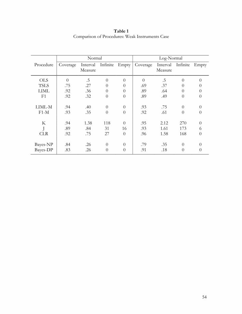
54
Table 1 Comparison of Procedures: Weak Instruments Case
Normal Log-Normal Procedure Coverage Interval
Measure Infinite Empty Coverage Interval
Measure Infinite Empty
OLS 0 .5 0 0 0 .5 0 0 TSLS .75 .27 0 0 .69 .37 0 0 LIML .92 .36 0 0 .89 .64 0 0
F1 .92 .32 0 0 .89 .49 0 0
LIML-M .94 .40 0 0 .93 .75 0 0 F1-M .93 .35 0 0 .92 .61 0 0
K .94 1.38 118 0 .95 2.12 270 0 J .89 .84 31 16 .93 1.61 173 6
CLR .92 .75 27 0 .96 1.58 168 0
Bayes-NP .84 .26 0 0 .79 .35 0 0 Bayes-DP .83 .26 0 0 .91 .18 0 0

55
Table 2 Comparison of Procedures: Moderate Instruments Case
Normal Log-Normal Procedure Coverage Interval
Measure Infinite Empty Coverage Interval
Measure Infinite Empty
OLS 0 .33 0 0 .01 .38 0 0 TSLS .89 .14 0 0 .86 .20 0 0 LIML .94 .15 0 0 .94 .23 0 0
F1 .94 .15 0 0 .94 .22 0 0
LIML-M .94 .15 0 0 .95 .24 0 0 F1-M .94 .15 0 0 .94 .23 0 0
K .93 .27 12 0 .94 .89 75 0 J .93 .20 0 7 .92 .42 9 9
CLR .94 .16 0 0 .94 .37 8 0
Bayes-NP .90 .13 0 0 .91 .19 0 0 Bayes-DP .90 .13 0 0 .92 .10 0 0

56
Table 3 Comparison of Procedures: Strong Instruments Case
Normal Log-Normal Procedure Coverage Interval
Measure Infinite Empty Coverage Interval
Measure Infinite Empty
OLS .06 .20 0 0 .03 .29 0 0 TSLS .92 .09 0 0 .90 .14 0 0 LIML .96 .10 0 0 .96 .15 0 0
F1 .95 .10 0 0 .96 .14 0 0
LIML-M .95 .10 0 0 .96 .15 0 0 F1-M .95 .09 0 0 .96 .14 0 0
K .94 .15 9 0 .93 .45 41 0 J .92 .17 0 11 .90 .24 0 13
CLR .94 .10 0 0 .95 .16 0 0
Bayes-NP .94 .09 0 0 .93 .13 0 0 Bayes-DP .92 .09 0 0 .96 .07 0 0
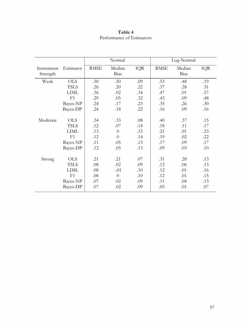
57
Table 4 Performance of Estimators
Normal Log-Normal
Instrument Strength
Estimator RMSE Median Bias
IQR RMSE Median Bias
IQR
Weak OLS .50 .50 .09 .53 .48 .19 TSLS .26 .20 .22 .37 .28 .31 LIML .36 .02 .34 .47 .01 .57 F1 .29 .05 .32 .43 .09 .48 Bayes-NP .24 .17 .23 .35 .26 .30
Bayes-DP .24 .18 .22 .16 .09 .16
Moderate OLS .34 .33 .08 .40 .37 .15 TSLS .12 .07 .14 .18 .11 .17 LIML .13 0 .15 .21 .01 .23 F1 .12 0 .14 .19 .02 .22 Bayes-NP .11 .05 .13 .17 .09 .17 Bayes-DP .12 .05 .13 .09 .03 .10
Strong OLS .21 .21 .07 .31 .28 .13 TSLS .08 .02 .09 .12 .06 .13 LIML .08 -.01 .10 .12 .01 .16 F1 .08 0 .10 .12 .01 .15 Bayes-NP .07 .02 .09 .11 .04 .13 Bayes-DP .07 .02 .09 .05 .01 .07

58
Table 5 Prior Sensitivity Analysis
Normal Log-Normal
Instrument Strength Prior Coverage Interval
Measure Coverage Interval Measure
Weak Default .83 .26 .91 .18 Alt 1 .74 .26 .85 .23 Alt 2 .74 .26 .86 .21
Moderate Default .90 .13 .92 .10 Alt 1 .87 .13 .93 .12 Alt 2 .88 .13 .92 .12
Strong Default .92 .09 .96 .07 Alt 1 .92 .09 .94 .09 Alt 2 .92 .09 .95 .08
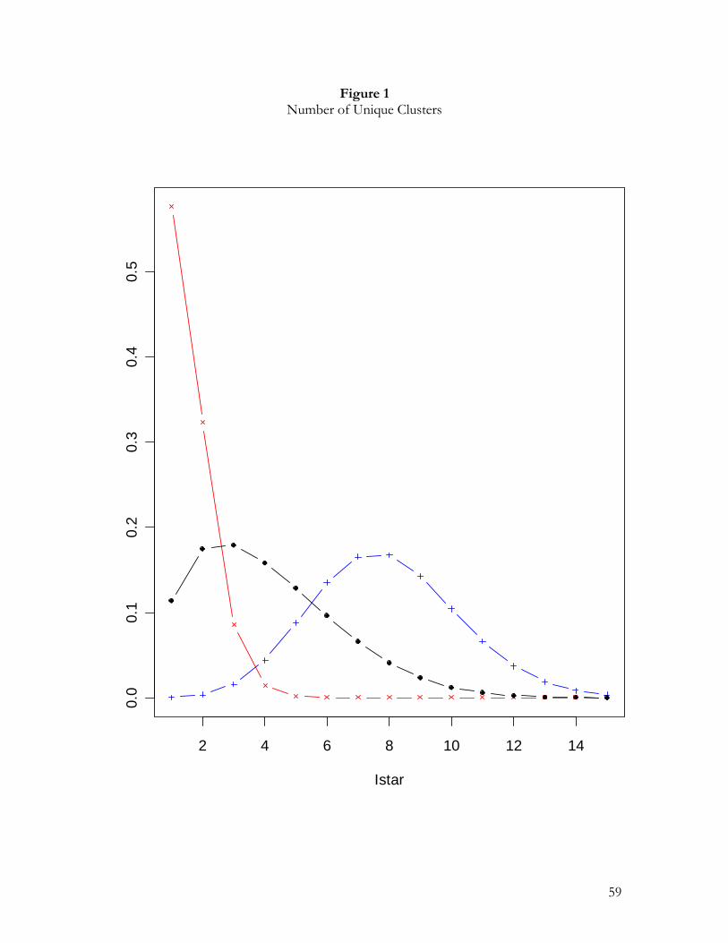
59
2 4 6 8 10 12 14
0.0
0.1
0.2
0.3
0.4
0.5
Istar
Figure 1 Number of Unique Clusters

60
Figure 2 Posterior Distribution of the Structural Coefficient: Acemoglu Data
Bayes with Nomal Errors
posterior mean = 0.752beta
-1 0 1 2
050
010
0020
0030
00
[ ]
posterior mean = 0.997beta
-1 0 1 2
010
0020
0030
0040
0050
00
[ ]
Bayes with DP Prior

61
-2 -1 0 1 2
-2-1
01
2
e1
e2
Figure 3 Fitted Error Density: Acemoglu Data

62
Figure 4 Posterior Distribution of the Structural Coefficient: Card Data
Bayes with Normal Errors
posterior mean = 0.185beta
0.0 0.1 0.2 0.3 0.4 0.5
050
010
0015
0020
0025
00
[ ]
posterior mean = 0.105beta
0.0 0.1 0.2 0.3 0.4 0.5
050
010
0015
0020
00
[ ]
Bayes with DP Prior

63
Figure 5 Fitted Error Densities: Card Data
-2 -1 0 1 2
-2-1
01
2
e1
e2
-2 -1 0 1 2
-2-1
01
2
e1
e2
One Component Normal
DP Prior
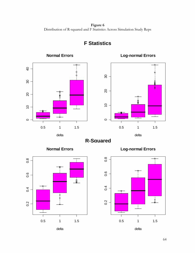
64
Figure 6 Distribution of R-squared and F Statistics Across Simulation Study Reps
F Statistics
R-Squared
0.5 1 1.5
010
2030
40
Normal Errors
delta
0.5 1 1.5
010
2030
Log-normal Errors
delta
0.5 1 1.5
0.2
0.4
0.6
0.8
Normal Errors
delta
0.5 1 1.5
0.2
0.4
0.6
0.8
Log-normal Errors
delta
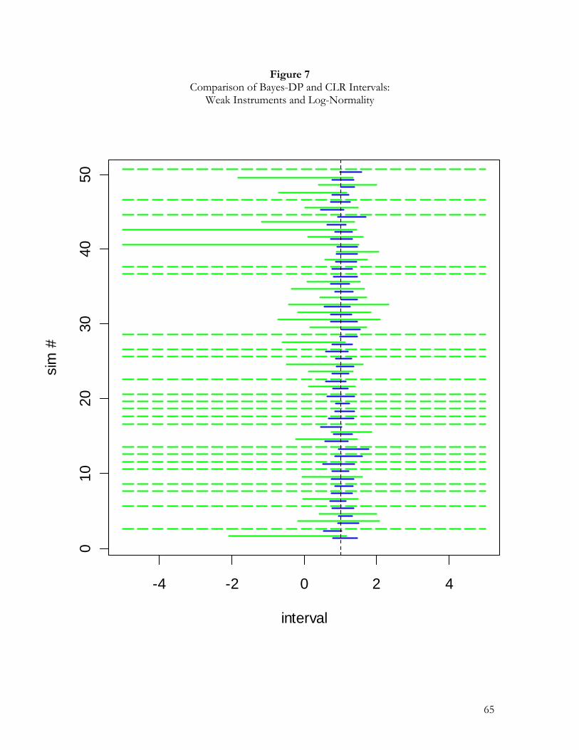
65
-4 -2 0 2 4
010
2030
4050
interval
sim
#Figure 7
Comparison of Bayes-DP and CLR Intervals: Weak Instruments and Log-Normality

66
-4 -2 0 2 4
010
2030
4050
interval
sim
#Figure 8
Comparison of Bayes-DP and F1-M Intervals: Weak Instruments and Log-Normality
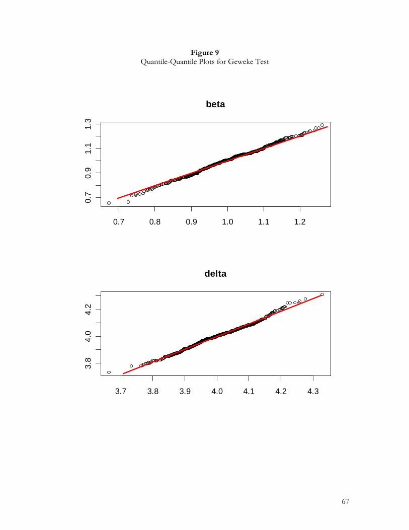
67
0.7 0.8 0.9 1.0 1.1 1.2
0.7
0.9
1.1
1.3
beta
3.7 3.8 3.9 4.0 4.1 4.2 4.3
3.8
4.0
4.2
delta
Figure 9 Quantile-Quantile Plots for Geweke Test


