
A Software-Defined Radio for the Masses, Part 1
This series describes a complete PC-base~ software-defined radio that uses a sound card and an innovative detector
circuit. Mathematics is minimized in the explanation. Come see how it's done.
Acertain convergence occurs when multiple technologies align in time to make possible
those things that once were only dreamed. The explosive growth of the Internet starting in 1994 was one of those events. While the Internet had existed for many years in government and education prior to that, its popularity had never crossed over into the general populace because of its slow speed and arcane interface. The development of the Web browser, the rapidly accelerating power and availability of the PC, and the availability of inexpensive and increasingly
8900 Marybank Dr Austin, TX 78750 [email protected]
By Gerald Youngblood, AC50G
speedy modems brought about the Internet convergence. Suddenly, it all came together so that the Internet and the worldwide Web joined the everyday lexicon of our society.
A similar convergence is occurring in radio communications through digital signal processing (DSP) software to perform most radio functions at performance levels previously considered unattainable. DSP has now been incorporated into much of the amateur radio gear on the market to deliver improved noise-reduction and digital-filtering performance. More recently, there has been a lot ofdiscussion about the emergence of so-called software-defined radios (SDRs).
A software-defined radio is characterized by its flexibility: Simply modifying or replacing software programs
can completely change its functionality. This allows easy upgrade to new modes and improved performance without the need to replace hardware. SDRs can also be easily modified to accommodate the operating needs of individual applications. There is a distinct difference between a radio that internally uses software for some of its functions and a radio that can be completely redefined in the field through modification of software. The latter is a software-defined radio.
This SDR convergence is occurring because of advances in software and silicon that allow digital processing of radio-frequency signals. Many of these designs incorporate mathematical functions into hardware to perform all ofthe digitization, frequency selection, and down-conversion to base-
q~ Jul/Aug 2002 13 76

band. Such systems can be quite complex and somewhat out of reach to most amateurs.
One problem has been that unless you are a math wizard and proficient in programming C++ or assembly language, you are out ofluck. Each can be somewhat daunting to the amateur as well as to many professionals. Two years ago, I set out to attack this challenge armed with a fascination for technology and a 25-year-old, virtually unused electrical engineering degree. I had studied most of the math in college and even some of the signal processing theory, but 25 years is a long time. I found that it really was a challenge to learn many of the disciplines required because much of the literature was written from a mathematician's perspective.
Now that I am beginning to grasp many of the concepts involved in software radios, I want to share with the Amateur Radio community what I have learned without using much more than simple mathematical concepts. Further, a software radio should have as little hardware as possible. If you have a PC with a sound card, you already have most of the required hardware. With as few as three integrated circuits you can be up and running with a Tayloe detectoran innovative, yet simple, direct-conversion receiver. With less than a dozen chips, you can build a transceiver that will outperform much of the commercial gear on the market.
Approach the Theory
In this article series, I have chosen to focus on practical implementation rather than on detailed theory. There are basic facts that must be understood to build a software radio. However, much like working with integrated circuits, you don't have to know how to create the IC in order to use it in a design. The convention I have chosen is to describe practical applications followed by references where appropriate for more detailed study. One of the easier to comprehend references I have found is The Scientist and Engineer's Guide to Digital Signal Processing by Steven W. Smith. It is free for download over the Internet at www.DSPGuide. com. I consider it required reading for those who want to dig deeper into implementation as well as theory. I will refer to it as the "DSP Guide" many times in this article series for further study.
So get out your four-function calculator (okay, maybe you need six or
14 Jul/Aug 2002 a~
seven functions) and let's get started. But first, let's set forth the objectives of the complete SDR design: • Keep the math simple • Use a sound-card equipped PC to pro
vide all signal-processing functions • Program the user interface and all
signal-processing algorithms in Visual Basic for easy development and maintenance
• Utilize the Intel Signal Processing Library for core DSP routines to minimize the technical knowledge requirement and development time, and to maximize performance
• Integrate a direct conversion (D-C) receiver for hardware design simplicity and wide dynamic range
• Incorporate direct digital synthesis (DDS) to allow flexible frequency control
• Include transmit capabilities using similar techniques as those used in the D-C receiver.
Analog and Digital Signals in the Time Domain
To understand DSP we first need to understand the relationship between digital signals and their analog counterparts. If we look at a I-V (pk) sine wave on an analog oscilloscope, we see that the signal makes a perfectly smooth curve on the scope, no matter how fast the sweep frequency. In fact, ifit were possible to build a scope with an infinitely fast horizontal sweep, it would still display a perfectly smooth curve (really a straight line at that point). As such, it is often called a continuous-time signal since it is continuous in time. In other words, there are an infinite number of different voltages along the curve, as can be seen on the analog oscilloscope trace.
On the other hand, if we were to measure the same sine wave with a digital voltmeter at a sampling rate of four times the frequency of the sine wave, starting at time equals zero, we wouldread:OVatO·, 1 Vat90·,OVat 1800 and -1 V at 270 0 over one complete cycle. The signal could continue perpetually, and we would still read those same four voltages over and again, forever. We have measured the voltage of the signal at discrete moments in time. The resulting voltagemeasurement sequence is therefore called a discrete-time signal.
Ifwe save each discrete-time signal voltage in a computer memory and we know the frequency at which we sampled the signal, we have a discretetime sampled signal. This is what an analog-to-digital converter (ADC)
does. It uses a sampling clock to measure discrete samples of an incoming analog signal at precise times, and it produces a digital representation of the input sample voltage.
In 1933, Harry Nyquist discovered that to accurately recover all the components of a periodic waveform, it is necessary to use a sampling frequency of at least twice the bandwidth of the signal being measured. That minimum sampling frequency is called the Nyquist criterion. This may be expressed as:
Is ~ 2/bw (Eq 1)
wherefs is the sampling rate andfbw is the bandwidth. See? The math isn't so bad, is it?
Now as an example of the Nyquist criterion, let's consider human hearing, which typically ranges from 20 Hz to 20 kHz. To recreate this frequency response, a CD player must sample at a frequency of at least 40 kHz. As we will soon learn, the maximum frequency component must be limited to 20 kHz through low-pass filtering to prevent distortion caused by false images of the signal. To ease filter requirements, therefore, CD players use a standard samplingrateof44,100 Hz. All modern PC sound cards support that sampling rate.
What happens if the sampled bandwidth is greater than halfthe sampling rate and is not limited by a low-pass filter? An alias ofthe signal is produced that appears in the output along with the original signal. Aliases can cause distortion, beat notes and unwanted spurious images. Fortunately, alias frequencies can be precisely predicted and prevented with proper low-pass or band-pass filters, which are often referred to as anti-aliasing filters, as shown in Fig 1. There are even cases where the alias frequency can be used to advantage; that will be discussed later in the article.
This is the point where most texts on DSP go into great detail about what sampled signals look like above the Nyquist frequency. Since the goal of this article is practical implementation, I refer you to Chapter 3 of the DSP Guide for a more in-depth discussion of sampling, aliases, A-to-D and
LPF
Signal
Fig 1-AID conversion with antialiaslng low-pass filter.
77

D-to-A conversion. Also refer to Doug Smith's article, "Signals, Samples, and Stuff: A DSP Tutorial."l
What you need to know for now is that ifwe adhere to the Nyquist criterion in Eq 1, we can accurately sample, process and recreate virtually any desired waveform. The sampled signal will consist of a series of numbers in computer'memory measured at time intervals equal to the sampling rate. Since we now know the amplitude of the signal at discrete time intervals, we can process the digitized signal in software with a precision and flexibility not possible with analog circuits.
From RF to a PC's Sound Card
Our objective is to convert a modulated radio-frequency signal from the frequency domain to the time domain for software processing. In the frequency domain, we measure amplitude versus frequency (as with a spectrum analyzer); in the time domain, we measure amplitude versus time (as with an oscilloscope).
In this application, we choose to use a standard 16-bit PC sound card that has a maximum sampling rate of 44,100 Hz. According to Eq 1, this means that the maximum-bandwidth signal we can accommodate is 22,050 Hz. With quadrature sampling, discussed later, this can actually be extended to 44 kHz. Most sound cards have built-in antialiasing filters that cut off sharply at around 20 kHz. (For a couple hundred dollars more, PC sound cards are now available that support 24 bits at a 96-kHz sampling rate with up to 105 dB of dynamic range.)
Most commercial and amateur DSP designs use dedicated DSPs that sample intermediate frequencies (lFs) of 40 kHz or above. They use traditional analog superheterodyne techniques for down-conversion and filtering. With the advent of very-high-speed and wide-bandwidth ADCs, it is now possible to directly sample signals up through the entire HF range and even into the low VHF range. For example, the Analog Devices AD9430 AID converter is specified with sample rates up to 210 Msps at 12 bits of resolution and a 700-MHz bandwidth. That 700-MHz bandwidth can be used in under-sampling applications, a topic that is beyond the scope of this article series.
The goal of my project is to build a PC-based softwaredefined radio that uses as little external hardware as possible while maximizing dynamic range and flexibility. To do so, we will need to convert the RF signal to audio frequencies in a way that allows removal of the unwanted mixing products or images caused by the down-conversion process. The simplest way to accomplish this while maintaining wide dynamic range is to use D-C techniques to translate the modulated RF signal directly to baseband.
'Notes appear on page 21.
LPF 1.5 kHz
14.001 MHz _~ Baseband
~ "OMH'
We can mix the signal with an oscillator tuned to the RF carrier frequency to translate the bandwidth-limited signal to a O-Hz IF as shown in Fig 2.
The example in the figure shows a 14.001-MHz carrier signal mixed with a 14.000-MHz local oscillator to translate the carrier to 1 kHz. If the low-pass filter had a cutoff of 1.5 kHz, any signal between 14.000 MHz and 14.0015 MHz would be within the passband of the direct-conversion receiver. The problem with this simple approach is that we would also simultaneously receive all signals between 13.9985 MHz and 14.000 MHz as unwanted images within the passband, as illustrated in Fig 3. Why is that?
Most amateurs are familiar with the concept of sum and difference frequencies that result from mixing two signals. When a carrier frequency, fe' is mixed with a local oscillator, flo' they combine in the general form:
feflo =~[(fe + flo)+(fe - flo)] (Eq 2)
When we use the direct-conversion mixer shown in Fig 2, we will receive these primary output signals:
fe + fIo = 14.001 MHz + 14.000 MHz = 28.001 MHz
f e - flo = 14.001 MHz -14.000 MHz = 0.001 MHz
Note that we also receive the image frequency that "folds over" the primary output signals:
-fe + flo =-14.001 MHz+14.000 MHz=-O.OOI MHz
A low-pass filter easily removes the 28.001-MHz sum frequency, but the -O.OOl-MHz difference-frequency image will remain in the output. This unwanted image is the lower sideband with respect to the 14.000-MHz carrier frequency. This would not be a problem if there were no signals below 14.000 MHz to interfere. As previously stated, all undesired signals between 13.9985 and 14.000 MHz will translate into the passband along with the desired signals above 14.000 MHz. The image also results in increased noise in the output.
So how can we remove the image-frequency signals? It can be accomplished through quadrature mixing. Phasing or quadrature transmitters and receivers-also called Weaver-method or image-rejection mixers-have existed since the early days of single sideband. In fact, my first SSB transmitter was a used Central Electronics 20A exciter that incorporated a phasing design. Phasing systems lost favor in the early 1960s with the advent ofrelatively inexpensive, high-performance filters.
To achieve good opposite-sideband or image suppression, phasing systems require a precise balance of amplitude and phase between two samples of the signal that are 90° out
Image Signals Real Signals
-28.001 MHz -1 kHz 1 kHz 28.001 MHz
_ __----;1!1lL(I
t -l\1,f1--
'
t
Fig 3-0utput spectrum of a real mixer illustrating the sum,Fig 2-A direct-conversion real mixer with a 1.5-kHz low-pass difference and image frequencies.filter.
q~ Jul/Aug 2002 1578

of phase or in quadrature with each other-~orthogonal"is the term used in some texts. Until the advent of digital signal processing, it was difficult to realize the level of image rejection performance required ofmodern radio systems in phasing designs. Since digital signal processing allows precise numerical control of phase and amplitude, quadrature modulation and demodulation are the preferred methods. Such signals in quadrature allow virtually any modulation method to be implemented in software using DSP techniques.
Give Me I and Q and I Can Demodulate Anything
First, consider the direct-conversion mixer shown in Fig 2. When the RF signal is converted to baseband audio using a single channel, we can visualize the output as varying in amplitude along a single axis as illustrated in Fig 4. We will refer to this as the inphase or I signal. Notice that its magnitude varies from a positive value to a negative value at the frequency of the modulating signal. Ifwe use a diode to rectify the signal, we would have created a simple envelope or AM detector.
Remember that in AM envelope detection, both modulation sidebands carry information energy and both are desired at the output. Only amplitude information is required to fully de
of the squares of the other two sidesaccording to the Pythagorean theorem. Or restating, the hypotenuse as mt (magnitude with respect to time):
(Eq 3)
The instantaneous phase ofthe signal as measured counterclockwise from the positive I axis and may be computed by the inverse tangent (or arctangent) as follows:
1¢t = tan-1 [ 7) (Eq 4)
1
Therefore, if we measured the instantaneous values of I and Q, we would know everything we needed to know about the signal at a given moment in time. This is true whether we are dealing with continuous analog signals or discrete sampled signals. With I and Q, we can demodulate AM signals directly using Eq 3 and FM signals using Eq 4. To demodulate SSB takes one more step. Quadrature signals can be used analytically to remove the image frequencies and leave only the desired sideband.
The mathematical equations for quadrature signals are difficult but are very understandable with a little study.2 I highly recommend that you read the online article, "Quadrature
Signals: Complex, But Not Complicated," by Richard Lyons. It can be found at www.dspguru.comlinfo/ tutor/quadsig.htm. The article develops in a very logical manner how quadrature-sampling l/Q demodulation is accomplished. A basic understanding ofthese concepts is essential to designing software-defined radios.
We can take advantage of the analytic capabilities of quadrature signals through a quadrature mixer. To understand the basic concepts of quadrature mixing, refer to Fig 6, which illustrates a quadrature-sampling IIQ mixer.
First, the RF input signal is bandpass filtered and applied to the two parallel mixer channels. By delaying the local oscillator wave by 90·, we can generate a cosine wave that, in tandem, forms a quadrature oscillator. The RF carrier, fc(t), is mixed with the respective cosine and sine wave local oscillators and is subsequently low-pass filtered to create the in-phase, l(t), and quadrature, Q(t), signals. The Q(t)
o
modulate the original signal. The problem is that most other modulation techniques require that the phase of the signal be known. This is where quadrature detection comes in. If we delay a copy ofthe RF carrier by 90 0 to form a quadrature (Q) signal, we can then use it in conjunction with the original in-phase signal and the math we learned in middle school to determine the instantaneous phase and amplitude of the original signal.
Fig 5 illustrates an RF carrier with the level of the I signal plotted on the x-axis and that ofthe Q signal plotted on the y-axis of a plane. This is often referred to in the literature as a phasor diagram in the complex plane. We are now able to extrapolate the two signals to draw an arrow or phasor that represents the instantaneous magnitude and phase of the original signal.
Okay, here is where you will have to use a couple of those extra functions on the calculator. To compute the magnitude mt or envelope of the signal, we use the geometry of right triangles. In a right triangle, the square ofthe hypotenuse is equal to the sum
16 JullAug 2002 q~
o-------.i---__- In Phase
Fig 4-An in-phase signal (I) on the real plane.The magnitude, m(t)1 is easily measured as the instantaneous peak voltage, but no phase information is available from in-phase detection.This is the wayan AM envelope detector works.
Fig 5--1 +jQ are shown on the complex plane.The vector rotates counterclockwise at a rate of 21tf ' The magnitude and cphase of the rotating vector at any instant in time may be determined through Eqs 3 and 4.
I(t)
Ott)
Fig 6-Ouadrature sampling mixer: The RF carrier, 'c- is fed to parallel mixers. The local oscillator (Sine) is fed to the lower-ehannel mixer directly and Is delayed by 90· (Cosine) to feed the upper-ehannel mixer.The low-pass filters provide antiallas filtering before analog-to-digital conversion. The upper channel provides the In-phase (/(1» signal and the lower channel provides the quadrature (Q.m2signaL In the PC SDR the low-pass filters and AID converters are integrated on the PC sound card.
79

channel is phase-shifted 90· relative to the I(t) channel through mixing with the sine local oscillator. The low-pass filter is designed for cutoff below the Nyquist frequency to prevent aliasing in the AID step. The AID converts continuous-time signals to discrete-time sampled signals. Now that we have the I and Q samples in memory, we can perform the magic of digi tal signal processing.
Before we go further, let me reiterate that one of the problems with this method of down-conversion is that it can be costly to get good opposite-sideband suppression with analog circuits. Any variance in component values will cause phase or amplitude imbalance between two channels, resulting in a corresponding decrease in oppositesideband suppression. With analog circuits, it is difficult to achieve better than 40 dB of suppression without much higher cost. Fortunately, it is straightforward to correct the analog imbalances in software.
Another significant drawback of direct-conversion receivers is that the noise increases as the demodulated signal approaches 0 Hz. Noise contributions come from a number of sources, such as 11fnoise from the semiconductor devices themselves, 60-Hz and 120-Hz line noise or hum, microphonic mechanical noise and local-oscillator phase noise near the carrier frequency. This can limit sensitivity since most people prefer their CW tones to be below 1 kHz. It turns out that most of the low-frequency noise rolls off above 1 kHz. Since a sound card can process signals all the way up to 20 kHz, why not use some ofthat bandwidth to move away from the low frequency noise? The PC SDR uses an 11.025-kHz, offsetbaseband IF to reduce the noise to a manageable level. By offsetting the local oscillator by 11.025 kHz, we can now receive signals near the carrier
frequency without any of the lowfrequency noise issues. This also significantly reduces the effects of local-oscillator phase noise. Once we have digitally captured the signal, it is a trivial software task to shift the demodulated signal down to a O-Hz offset.
DSP in the Frequency Domain Every DSP text I have read thus far
concentrates on time-domain filtering and demodulation of SSB signals using finite-impuLse-response (FIR) filters. Since these techniques have been thoroughly discussed in the literature l , 3,4 and are not currently used in my PC SDR, they will not be covered in this article series.
My PC SDR uses the power of the fast Fourier transform (FFT) to do almost all of the heavy lifting in the frequency domain. Most DSP texts use a lot of ink to derive the math so that one can write the FFTcode. Since Intel has so helpfully provided the code in executable form in their signal-processing librarY,5 we don't care how to write an FFT: We just need to know how to use it. Simply put, the FFT converts the complex I and Q discrete-time signals into the frequency domain. The FFT output can be thought of as a large bank of very narrow band-pass filters, called bins, each one measuring the spectral energy within its respective bandwidth. The output resembles a comb filter wherein each bin slightly overlaps its adj acent bins forming a scalloped curve, as shown in Fig 7. When a signal is precisely at the cen ter frequency of a bin, there will be a corresponding value only in that bin. As the frequency is offset from the bin's center, there will be a corresponding increase in the value of the
adjacent bin and a decrease in the value of the current bin. Mathematical analysis fully describes the relationship between FFT bins,6 but such is beyond the scope of this article,
Further, the FFT allows us to measure both phase and amplitude of the signal within each bin using Eqs 3 and 4 above. The complex version allows us to measure positive and negative frequencies separately. Fig 8 illustrates the output of a complex, or quadrature, FFT.
The bandwidth of each FFT bin may be computed as shown in Eq 5, where BWbin is the bandwidth ofa single bin, fs is the sampling rate and N is the size of the FFT. The center frequency of each FFT bin may be determined by Eq 6 where feenter is the bin's center frequency, n is the bin number,{s is the sampling rate and N is the size of the FFT. Bins zero through (N/2)-l represent upper-sideband frequencies and bins N/2 to N-1 represent lower-sideband frequencies around the carrier frequency.
BWbin = Is N
(Eq 5)
nls leenler =N (Eq 6)
If we assume the sampling rate of the sound card is 44.1 kHz and the number of FFT bins is 4096, then the bandwidth and center frequency of each bin would be:
44100BWb'n = -- = 10.7666 Hz and
I 4096
Icenler = nlO.7666 Hz
What this all means is that the receiver will have 4096, -ll-Hz-wide
Ie nls
Center~ N
Frequency
Fig 7-FFT output resembles a comb filter: Each bin of the FFT overlaps its adjacent bins just as in a comb filter. The 3·dB points overlap to provide linear output. The phase and magnitude of the signal in each bin is easily determined mathematically with Eqs 3 and 4.
~~~~ t LSB USB t N !::! _ 1 2 2
(Bin 2048) (Bin 2047)
Fig 8-Complex FFT output: The output of a. complex FFT may b~ thought of as a series of band-pass filters aligned around the carner frequency, fe' at bm O. N represents the number of FFT bins. The upper sideband is located in bins 1 through (N/2}-1 a.nd the lower sideband is located in bins N/2 to ~1.The center frequency and bandWidth of each bin may be calculated using Eqs 5 and 6.
QE*o-- JullAug 2002 17 80

band-pass filters. We can therefore create band-pass filters from 11 Hz to
LMS Noiseapproximately 40 kHz in 11-Hz steps. & Notch
The PC SDR performs the following Q Filter functions in the frequency domain after FFT conversion: • Brick-wall fixed and variable band-
pass filters • Frequency conversion • SSB/CW demodulation • Sideband selection • Frequency-domain noise subtraction • Frequency-selective squelch • Noise blanking • Graphic equalization ("tone control") • Phase and amplitude balancing to
remove images
2048 Taps
Amplitude & Phase
Correction
DigitalAGC 1 ms Attack
100,200,300 ms Hold
• SSB generation • Future digital modes such as PSK31
and RTTY Once the desired frequency-domain
processing is completed, it is simple to convert the signal back to the time domain by using an inverse FFT. In the PC SDR, only AGC and adaptive noise filtering are currently performed in the time domain. A simplified diagram of the PC SDR software architecture is provided in Fig 9. These concepts will be discussed in detail in a future article.
Sampling RF Signals with the Tayloe Detector: A New Twist on an Old Problem
While searching the Internet for information on quadrature mixing, I ran across a most innovative and elegant design by Dan Tayloe, N7VE. Dan, who works for Motorola, has developed and patented (US Patent #6,230,000) what has been called the Tayloe detector7 . The beauty of the Tayloe detector is found in both its design elegance and its exceptional performance. It resembles other concepts in design, but appears unique in its high performance with minimal components.B, 9, 10, 11 In its simplest form, you can build a complete quadrature down converter with only three or four ICs (less the local oscillator) at a cost ofless than $10.
Fig 10 illustrates a single-balanced version of the Tayloe detector. It can be visualized as a four-position rotary switch revolving at a rate equal to the carrier frequency. The 50-n antenna impedance is connected to the rotor and each of the four switch positions is connected to a sampling capacitor. Since the switch rotor is turning at exactly the RF carrier frequency, each capacitor will track the carrier's amplitude for exactly one-quarter of the cycle and will hold its value for the remainder of
18 JullAug 2002 q~
Fig 9-SDR receiver software architecture: The I and Q signals are fed from the soundcard input directly to a 40gB-bin complex FFT. Band-pass filter coefficients are precomputed and converted to the frequency domain using another FFT.The frequencydomain filter is then mUltiplied by the frequency-domain signal to provide brick-wall filtering. The filtered signal Is then converted to the time domain using the Inverse FFT. Adaptive noise and notch filtering and digital AGC follow In the time domain.
~-------l
I 50 Ohm Antenna 1 O'I
I I I I 1 I I Q ' 1
to provide the quadrature (0) signal.
the cycle. The rotating switch will therefore sample the signal at 0·, 90·, 180· and 270·, respectively.
As shown in Fig 11, the 50-n impedance of the antenna and the sampling capacitors form an R-C low-pass filter during the period when each respective switch is turned on. Therefore, each sample represents the integral or average voltage ofthe signal during its respective one-quarter cycle. When the switch is off, each sampling capacitor will hold its value until the next revolution. If the RF carrier and the rotating frequency were exactly in phase, the output of each capacitor will be a dc level equal to the average
...-Jov'Vv--c-r I o-y--C>--i Baseband
I 1'c I rt7 5
~
Fig 11-Track and hold sampling circuit: Each of the tour sampling capacitors in the Tayloe detector form an RC track-and-hold circuit. When the switch Is on, the capacitor will charge to the average value of the carrier during its respective onequarter cycle. During the remaining threequarters cycle, It will hold its charge. The local-oscillator frequency Is equal to the carrier frequency so that the output will be at baseband.
Fig 1G-Tayloe detector: The switch rotates at the carrier frequency so that each capacitor samples the signal once each revolution. The 0" and 180" capacitors differentially sum to provide the In-phase (I) signal and the 90· and 270· capacitors sum
81
--
--
value of the sample. If we differentially sum outputs of
the 0° and 180° sampling capacitors with an op amp (see Fig 10), the output would be a dc voltage equal to two times the value of the individually sampled values when the switch rotation frequency equals the carrier frequency. Imagine, 6 dB of noise-free gain! The same would be true for the 90° and 270° capacitors as well. The 0°/180° summation forms the] channel and the 90°/270° summation forms the Q channel ofthe quadrature downconversion.
As we shift the frequency of the carrier away from the sampling frequency, the values of the inverting phases will no longer be dc levels. The output frequency will vary according to the "beat" or difference frequency between the carrier and the switch-rotation frequency to provide an accurate representation of all the signal
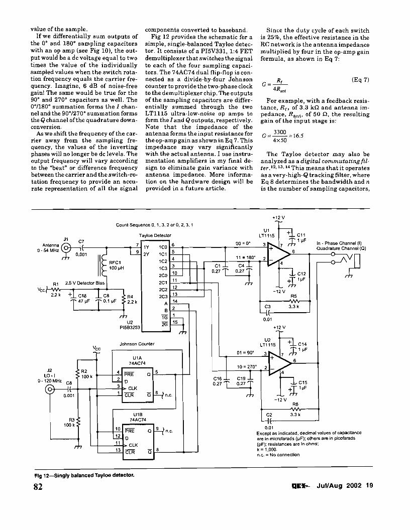
components converted to baseband. Fig 12 provides the schematic for a
simple, single-balanced Tayloe detector. It consists of a P15V331, 1:4 FET demultiplexer that switches the signal to each of the four sampling capacitors. The 74AC74 dual flip-flop is connected as a divide-by-four Johnson counter to provide the two-phase clock to the demultiplexer chip. The outputs of the sampling capacitors are differentially summed through the two LT1l15 ultra-low-noise op amps to form the] and Q outputs, respectively. Note that the impedance of the antenna forms the input resistance for the op-amp gain as shown in Eq 7. This impedance may vary significantly with the actual antenna. I use instrumentation amplifiers in my final design to eliminate gain variance with antenna impedance. More information on the hardware design will be provided in a future article.
Since the duty cycle of each switch is 25%, the effective resistance in the RC network is the antenna impedance multiplied by four in the op-amp gain formula, as shown in Eq 7:
(Eq 7)
For example, with a feedback resistance, R rf of 3.3 k12 and antenna impedance, Rant' of 50 12, the resulting gain of the input stage is:
G = 3300 =16.5 4x50
The Tayloe detector may also be analyzed as a digital commutating filter .12,13,14 This means that it operates as a very-high-Q tracking filter, where Eq 8 determines the bandwidth and n is the number of sampling capacitors,
+12 V -~
U1 l T1115 8C11;+; 1 IJF00 =O· In - Phase Ch annel (I) 3~7 Ouadrature C hannel (0)
6 f'\.
-o...!'2~4
nC12
~1IJF-.... -12 V
R5
C3 3.3 k II
" 0.01
+12 V -~
U2 ~ lT1115 + C14;+; 1 IJF01 =90· ~7
6
~C15fh 1IJF
-12 V R6
C2 3.3 k
" 0.01 Except as indicated, decimal values of capacitance are in microfarads (IJF): others are in picof arads (pF): resistances are in ohms: k =1,000. n.C. =No connection
11 =180·
L. C4..L
0.27~
3 +
10 =270· 2 I:/' 4
C16 L. c191
0.27~
J1 C7 Antenna~
0- 54 MHz
R1 I
Vee « 2.2 k
J2 lO -I
0- 120 MHz
'V',/
Count Sequence O. 1, 3, 2 or 0, 2, 3, 1
Tayloe Detector
,J t RFC1
C1>- 100 IJH
0.001
R3 100 k
rI-T
7 61Y 1CO 5U 2Y 1C1 41C2 31C3
2CO .J-Q...112C1 122C2 13C8+ C18 R4 2C3
;1" 47 IJF '1" 0.1 IJF 142.2 k A 2B
U2 lG~2G 15 PI583253
Johnson Counter
U1A 74AC74
4 5PRE 0 L...1. 0
3 ClK 1 QClR ~n.c.
U1B 74AC74
10 -PRE o~n.c. .E.. 0
11 ClK 13 8QClR
2.5 V Detector Bia~
r7
Vee
R2 100 k
C8 If
1\
I~
0.001
Fig 12-Singly balanced Tayloe detector.
qE*s- JullAug 2002 1982

Rant is the antenna impedance and Cs is the value ofthe individual sampling capacitors. Eq 9 determines the Qdet of the filter, where fc is the center frequency and BWdet is the bandwidth of the filter.
(Eq 8)
Q ~ mqIDdet=-BW
det By example, if we assume the sam
pling capacitor to be 0.27 p.F and the antenna impedance to be 50 n, then BW and Q are computed as follows:
1 = = 5895 Hz BWdet
(Jr)(4)(50)(2.7XIO-7 )
6 n. = 14.001x10 = 2375 ~el 5895
Since the PC SDR uses an offset baseband IF, I have chosen to design the detector's bandwidth to be 40 kHz to allow low-frequency noise elimination as discussed above.
The real payoff in the Tayloe detector is its performance. It has been stated that the ideal commutating mixer has a minimum conversion loss (which equates to noise figure) of 3.9 dB.l5, 16 Typical high-level diode mixers have a conversion loss of6-7 dB and noise figures 1 dB higher than the loss. The Tayloe detector has less than 1 dB of conversion loss, remarkably. How can this be? The reason is that it is not really a mixer but a sampling detector in the form of a quadrature track and hold. This means that the design adheres to discrete-time sampling theory, which, while similar to mixing, has its own unique characteristics. Because a track and hold actually holds the signal value between samples, the signal output never goes to zero.
This is where aliasing can actually be used to our benefit. Since each switch and capacitor in the Tayloe detector actually samples the RF signal once each cycle, it will respond to alias frequencies as well as those within the Nyquist frequency range. In a traditional direct-conversion receiver, the local-oscillator frequency is set to the carrier frequency so that the difference frequency, or IF, is at 0 Hz and the sum frequency is at two times the carrier frequency per Eq 2. We normally remove the sum frequency through low-pass filtering, resulting in conversion loss and a corresponding
20 Jul/Aug 2002 q~
increase in noise figure. In the Tayloe detector, the sum frequency resides at the first alias frequency as shown in Fig 13. Remember that an alias is a real signal and will appear in the output as if it were a baseband signal. Therefore, the alias adds to the baseband signal for a theoretically lossless detector. In real life, there is a slight loss due to the resistance ofthe switch and aperture loss due to imperfect switching times.
PC SDR Transceiver Hardware
The Tayloe detector therefore provides a low-cost, high-performance method for both quadrature down-conversion as well as up-conversion for transmitting. For a complete system, we would need to provide analog AGC to prevent overload of the ADC inputs and a means of digital frequency control. Fig 14 illustrates the hardware
PC Control & I & a AUdio
Log Amplifier
AD8307
PI5V331
architecture ofthe PC SDR receiver as it currently exists. The challenge has been to build a low-noise analog chain that matches the dynamic range ofthe Tayloe detector to the dynamic range of the PC sound card. This will be covered in a future article.
I am currently prototyping a complete PC SDR transceiver, the SDR-I000, that will provide generalcoverage receive from 100 kHz to 54 MHz and will transmit on all ham bands from 160 through 6 meters.
SDR Applications At the time of this writing, the typi
cal entry-level PC now runs at a clock frequency greater than 1 GHz and costs only a few hundred dollars. We now have exceptional processing power at our disposal to perform DSP tasks that were once only dreams. The transfer of knowledge from the aca
o Alias Alias
Fig 13-Alias summing on Tayloe detector output: Since the Tayloe detector samples the signal the sum frequency (fc + fs) and Its Image (-fc - fs) are located at the first alias frequency.The alias signals sum with the baseband signals to eliminate the mixing product loss associated with traditional mixers. In a typical mixer, the sum frequency energy Is lost through filtering thereby increasing the noise figure of the device.
SSM2164
Audio
Fig 14-PC SDR receiver hardware architecture: After band-pass filtering the antenna is fed directly to the Tayloe detector, which In turn provides I and Q outputs at baseband. A DDS and a divide-by-four Johnson counter drive the Tayloe detector demultiplexer.The LT1115s offer ultra-low noise-differential summing and amplification prior to the widedynamic-range analog AGC circuit formed by the SSM2164 and AD830710g amplifier.
83
demic to the practical is the primary limit ofthe availability ofthis technology to the Amateur Radio experimenter. This article series attempts to demystify some of the fundamental concepts to encourage experimentation within our community. TheARRL recently formed a SDR Working Group for supporting this effort, as well.
The SDR mimics the analog world in digital data, which can be manipulated much more precisely. Analog radio has always been modeled mathematically and can therefore be processed in a computer. This means that virtually any modulation scheme may be handled digitally with performance levels difficult, or impossible, to attain with analog circuits. Let's consider some of the amateur applications for the SDR: • Competition-grade HF transceivers • High-performance IF for microwave
bands • Multimode digital transceiver • EME and weak-signal work • Digital-voice modes • Dream it and code it
For Further Reading For more in-depth study of DSP
techniques, I highly recommend that you purchase the following texts in order of their listing:
Understanding Digital Signal Processing by Richard G. Lyons (see Note 6). This is one of the best-written textbooks about DSP.
Digital Signal Processing Technology by Doug Smith (see Note 4). This new book explains DSP theory and application from an Amateur Radio perspective.
Digital Signal Processing in Communications Systems by Marvin E. Frerking (see Note 3). This book relates DSP theory specifically to modulation and demodulation techniques for radio applications.
Acknowledgements I would like to thank those who have
assisted me in my journey to understanding software radios. Dan Tayloe, N7VE, has always been helpful and responsive in answering questions about the Tayloe detector. Doug Smith, KF6DX, and Leif Asbrink, SM5BSZ, have been gracious to answer my questions about DSP and receiver design on numerous occasions. Most of all, I want to thank my Saturday-morning breakfast review team: Mike Pendley,
WA5VTV; Ken Simmons, K5UHF; Rick Kirchhof, KD5ABM; and Chuck McLeavy, WB5BMH. These guys put up with my questions every week and have given me tremendous advice and feedback all throughout the project. I also want to thank my wonderful wife, Virginia, who has been incredibly patient with all the hours I have put in on this project.
Where Do We Go From Here?
Three future articles will describe the construction and programming of the PC SDR. The next article in the series will detail the software interface to the PC sound card. Integrating fullduplex sound with DirectX was one of the more challenging parts of the project. The third article will describe the Visual Basic code and the use of the Intel Signal Processing Library for implementing the key DSP algorithms in radio communications. The final article will describe the completed transceiver hardware for the SDR1000.
Notes 1D. Smith, KF6DX, "Signals, Samples and
Stuff: A DSP Tutorial (Part 1)," QEX, Mar/ Apr 1998, pp 3-11.
2J. Bloom, KE3Z, "Negative Frequencies and Complex Signals," QEX, Sep 1994, pp 22-27.
3M. E. Frerking, Digital Signal Processing in Communication Systems (New York: Van Nostrand Reinhold, 1994, ISBN: 0442016166), pp 272-286.
4D. Smith, KF6DX, Digital Signal Processing Technology (Newington, Connecticut: ARRL, 2001), pp 5-1 through 5-38.
5The Intel Signal Processing Library is available for download at developer.lntel. com/software/products/perflib/spl/.
6R. G. Lyons, Understanding Digital Signal Processing, (Reading, Massachusetts: Addison-Wesley, 1997). pp 49-146.
7D. Tayloe, N7VE, "Letters to the Editor, Notes on'ldeal' Commutating Mixers (Nov/ Dec 1999)," QEX, March/April 2001, p 61.
8p. Rice, VK3BHR, "SSB by the Fourth Method?" available at ironbark.bendigo. latrobe.edu.au/-rice/ssb/ssb.html.
gA. A. Abidi, "Direct-Conversion Radio Transceivers lor Digital Communications," IEEE Journal of Solid-State CirCUits, Vol 30, No 12, December 1995, pp 13991410, Also on the Web at www.icsl.ucla. edu/aagroup/PDF_files/dir-con.pdf
10p. Y. Chan, A. Rolougaran, K.A. Ahmed, and A. A. Abidi, "A Highly Linear 1-GHz CMOS Downconversion Mixer." Presented at the European Solid State Circuits Conference, Seville, Spain, Sep 22-24, 1993, pp 210-213 of the conlerence proceedings. Also on the Web at www.icsl.ucla. edu/aagroup/PDF_files/mxr-93.pdf
11 D. H. van Graas, PA0DEN, "The Fourth Method: Generating and Detecting SSB Signals," QEX, Sep 1990, pp 7-11. This circuit is very similar to a Tayloe detector, but it has a lot of unnecessary components.
12M. Kossor, WA2EBY, "A Digital Commutating Filter," QEX, May/Jun 1999, pp 3-8.
13C. Ping, BA1 HAM, "An Improved Switched Capacitor Filter," QEX, Sep/Oct 2000, pp 41-45.
14p. Anderson, KC1HR, "Letters to the Editor, A Digital Commutating Filter," QEX, Jul/Aug 1999, pp 62.
15D. Smith, KF6DX, "Notes on 'Ideal' Commutating Mixers," QEX, Nov/Dec 1999, pp 52-54.
16p. Chadwick, G3RZP, "Letters to the Editor, Notes on 'Ideal' Commutating Mixers" (Nov/ Dec 1999), QEX, Mar/Apr 2000, pp 61-62.
Gerald became a ham in 1967 during high school, first as a Novice and then a General class as WA5RXV. He completed his Advanced class license and became KE50H before finishing high school and received his First Class Radiotelephone license while working in the television broadcast industry during college. After 25 years ofinactivity, Gerald returned to the active amateur ranks in 1997 when he completed the requirements for Extra class license and became AC50G.
Gerald lives in Austin, Texas, and is currently CEO of Sixth Market Inc, a hedge fund that trades equities using artificial-intelligence software. Gerald previously founded and ran five technology companies spanning hardware, software and electronic manufacturing. Gerald holds a Bachelor of Science Degree in Electrical Engineering from Mississippi Stage University.
Gerald is a member of the ARRL SDR working Group and currently enjoys homebrew software-radio development, 6-meter DX and satellite operations. DO
q~ Jul/Aug 2002 21 84

A Software-Defined Radio for the Masses, Part 2
Come learn how to use a PC sound card to enter the wondeiful world of digital signalprocessing.
By Gerald Youngblood, AC50G
Part 1 gave a general description of digital signal processing (nSP) in software-defined ra
dios (SDRs).l It also provided an overview of a full-featured radio that uses a personal computer to perform all DSP functions. This article begins design implementation with a complete description of software that provides a full-duplex interface to a standard PC sound card.
To perform the magic ofdigital signal processing, we must be able to convert a signal from analog to digital and back to analog again. Most amateur experimenters already have this ca
1Notes appear on page 18.
8900 Marybank Dr Austin, TX 78750 [email protected]
10 Sept/Oct 2002 q~
pability in their shacks and many have used it for slow-scan television or the new digital modes like PSK3l.
Part 1 discussed the power of quadrature signal processing using inphase <n and quadrature (Q) signals to receive or transmit using virtually any modulation method. Fortunately, all modem PC sound cards offer the perfect method for digitizing the I and Q signals. Since virtually all cards today provide 16-bit stereo at 44-kHz sampling rates, we have exactly what we need capture and process the signals in software. Fig 1 illustrates a direct quadrature-conversion mixer connection to a PC sound card.
This article discusses complete source code for a DirectX. sound-card interface in Microsoft Visual Basic. Consequently, the discussion assumes that the reader has some fundamen
tal knowledge of high-level language programming.
Sound Card and PC Capabilities Very early PC sound cards were low
performance, 8-bit mono versions. Today, virtually all PCs come with 16-bit stereo cards of sufficient quality to be used in a software-defined radio. Such a card will allow us to demodulate, filter and display up to approximatelya 44-kHz bandwidth, assuming a 44-kHz sampling rate. (The bandwidth is 44 kHz, rather than 22 kHz, because the use of two channels effectively doubles the sampling rate-Ed.) For high-performance applications, it is important to select a card that offers a high dynamic range-on the order of 90 dB. If you are just getting started, most PC sound cards will allow you to begin experimentation, although they
85

may offer lower performance. The best l6-bit price-to-perfor
mance ratio I have found at the time of this article is the Santa Cruz 6channel DSP Audio Accelerator from Turtle Beach Inc (www.tbeach.com). It offers four 18-bit internal analogto-digital (AJD) input channels and six 20-bit digital-to-analog (D/A) output channels with sampling rates up to 48 kHz. The manufacturer specifies a 96-dB signal-to-noise ratio (SNR) and better than -91 dB total harmonic distortion plus noise (THD+N). Crosstalk is stated to be -105 dB at 100 Hz. The Santa Cruz card can be purchased from online retailers for under $70.
Each bit on anAJD or D/A converter represents 6 dB of dynamic range, so a 16-bit converter has a theoretical limit of 96 dB. A very good converter with low-noise design is required to achieve this level of performance. Many l6-bit sound cards provide no more than 12-14 effective bits of dynamic range. To help achieve higher performance, the Santa Cruz card uses an 18-bit AID converter to deliver the 96 dB dynamic range (16-bit) specification.
A SoundBlaster 64 also provides reasonable performance on the order of76 dB SNR according to PC AV Tech at www.pcavtech.com. I have used this card with good results, but I much prefer the Santa Cruz card.
The processing power needed from the PC depends greatly on the signal processing required by the application. Since I am using very-high-performance filters and large fast-Fourier transforms (FFTs), my applications require at least a 400-MHz Pentium II processor with a minimum of 128 MB of RAM. If you require less performance from the software, you can get by with a much slower machine. Since the entry level for new PCs is now 1 GHz, many amateurs have ample processing power available.
Microsoft DirectX versus Windows Multimedia
Digital signal processing using a PC sound card requires that we be able to capture blocks ofdigitized I and Qdata through the stereo inputs, process those signals and return them to the soundcard outputs in pseudo real time. This is called full duplex. Unfortunately, there is no high-level software interface that offers the capabilities we need for the SDR application.
Microsoft now provides two application programming interfaces2 (APls) that allow direct access to the sound card under C++ and Visual Basic. The original interface is the Windows Mul
timedia system using the Waveform Audio API. While my early work was done with the Waveform Audio API, I later abandoned it for the higher performance and simpler interface DirectX offers. The only limitation I have found with DirectX is that it does not currently support sound cards with more than l6-bits of resolution. For 24-bit cards, Windows Multimedia is required. While the Santa Cruz card supports l8-bits internally, it presents only 16-bits to the interface. For information on where to download the DirectX software development kit (SDK) see Note 2.
Circular Buffer Concepts A typical full-duplex PC sound card
PC Control & 1& QAudio
Log Amplifier
AD8307
Tayloe Detector
PI5V331
Fig 1-Direct quadrature conversion mixer to sound-card interface used in the author's prototype.
o
I Play I~-T-_I- I Write
(B)
o
I Play +--7'-_-.1 I Write
6144
2048 0 BI
1 I ( \
I I \ I
2048 (A) DireclSoundCaptureBuffer
4096 (C) DirectSoundBuffer
Fig 2-DirectSoundCaptureBuffer and DirectSoundBuffer circular buffer layout.
q~ Sept/Oct 2002 11
allows the simultaneous capture and playback of two or more audio channels (stereo). Unfortunately, there is no high-level code in Visual Basic or
..
." '" . C++ to directly support full duplex as • required in an SDR. We will therefore have to write code to directly control the card through the DirectX API.
DirectX internally manages all lowlevel buffers and their respective interfaces to the sound-card hardware. Our code will have to manage the high-level DirectX buffers (called DirectSoundBuffer and DirectSoundCaptureBuffer) to provide uninterrupted operation in a multitasking system. The DirectSoundCaptureBuffer stores the digitized signals from the stereo
SSM2164
Audio
86

••••••
ND converter in a circular buffer and notifies the application upon the occurrence of predefined events. Once captured in the buffer, we can read the data, perform the necessary modulation or demodulation functions using DSP and send the data to the DirectSoundBuffer for D/A conversion and output to the speakers or transmitter.
To provide smooth operation in a multitracking system without audio popping or interruption, it will be necessary to provide a multilevel buffer for both capture and playback. You may have heard the term double buffering. We will use double buffering in the DirectS 0 undC a ptu reB uffer and quadruple buffering in the DirectSoundBuffer. I found that the quad buffer with overwrite detection was required on the output to prevent overwriting problems when the system is heavily loaded with other applications. Figs 2A and 2B illustrate the concept of a circular double buffer, which is used for the DirectSoundCaptureBuffer. Although the buffer is really a linear array in memory, as shown in Fig 2B, we can visualize it as circular, as illustrated in Fig 2A. This is so because DirectX manages the buffer so that as soon as each cursor reaches the end of the array, the driver resets the cursor to the beginning of the buffer.
The DirectSoundCaptureBuffer is broken into two blocks, each equal in size to the amount of data to be captured and processed between each event. Note that an event is much like an interrupt. In our case, we will use a block size of2048 samples. Since we are using a stereo (two-channel) board with 16 bits per channel, we will be capturing 8192 bytes per block (2048 samples x 2 channels x 2 bytes). Therefore, the DirectSoundCaptureBuffer will be twice as large (16,384 bytes).
Since the DirectSoundCapture Buffer is divided into two data blocks, we will need to send an event notification to the application after each block has been captured. The DirectX driver maintains cursors that track the position of the capture operation at all times. The driver provides the means of setting specific locations within the buffer that cause an event to trigger, thereby telling the application to retrieve the data. We may then read the correct block directly from the DirectSoundCaptureBuffer segment that has been completed.
Referring again to Fig 2A, the two cursors resemble the hands on a clock face rotating in a clockwise direction. The capture cursor, IPlay, represents the point at which data are currently
12 Sept/Oct 2002 q~
being captured. (I know that sounds backward, but that is how Microsoft defined it.) The read cursor, IWrite, trails the capture cursor and indicates the point up to which data can safely be read. The data after IWrite and up to and including IPlay are not necessarily good data because of hardware buffering. We can use the IWrite cursor to trigger an event that tells the software to read each respective block of data, as will be discussed later in the article. We will therefore receive two events per revolution of the circular buffer. Data can be captured into one half of the buffer while data are being read from the other half.
Fig 2C illustrates the DirectSoundBuffer, which is used to output data to the D/A converters. In this case, we will use a quadruple buffer to allow plenty of room between the currently playing segment and the segment being written. The play cursor, IPlay, always points to the next byte of data to be played. The write cursor, IWrite, is the point after which it is safe to write data into the buffer. The cursors may be thought of as rotating in a clockwise motion just as the capture cursors do. We must monitor the location of the cursors before writing to buffer locations between the cursors to prevent
overwriting data that have already been committed to the hardware for playback.
Now let's consider how the data maps from the DirectSoundCaptureBuffer to the DirectSoundBuffer. To prevent gaps or pops in the sound due to processor loading, we will want to fill the entire quadruple buffer before starting the playback looping. DirectX allows the application to set the starting point for the IPlay cursor and to start the playback at any time. Fig 3 shows how the data blocks map sequentially from the DirectSoundCaptureBuffer to the DirectSoundBuffer. Block 0 from the DirectSoundCaptureBuffer is transferred to Block 0 of the DirectSoundBuffer. Block 1 of the DirectSoundCaptureBuffer is next transferred to Block 1 of the DirectSoundBuffer and so forth. The subsequent source-code examples show how control of the buffers is accomplished.
Full Duplex, Step-by-Step The following sections provide a
detailed discussion of full-duplex DirectX implementation. The example code captures and plays back a stereo audio signal that is delayed by four
Fig 3-Method for mapping the DireclSoundCaplureBuffer
... Direct 1.0 Type Library [] DirectAnimation Library [] DirectShowStream 1.0 Type Library
0!iiiDilreicDtx,7~fomriv~isliuamlmB~asiicITilemLi~brlalir~!.!ooDmi 1.0 Type Library oDrawing Addin o drivers 1.0 Type Library o dsctl 1.0 Type Library odtcint 1.0 Type Library ODTC5erv 1.0 Type Library ODXTMsft 1.0 Type Library ODXTMsft3 1.0 Type Library
DirectSoundCaptureBuffer to the DlrectSoundBuffer.
Fig 4-Registration of the DirectX8 for Visual BasicType Library in the Visual Basic IDE.
87
capture periods through buffering. You should refer to the "DirectX Audio" section of the DirectX 8.0 Programmers Reference that is installed with the DirectX software developer's kit (SDK)throughout this discussion. The DSP code will be discussed in the next article of this series, which will discuss the modulation and demodulation ofquadrature signals in the SDR. Here are the steps involved in creating the DirectX interface: • Install DirectX runtime and SDK.
• Add a reference to DirectX8 for Visual Basic Type Library.
• Define Variables, I/O buffers and DirectX objects.
• Implement DirectX8 events and event handles.
• Create the audio devices. • Create the DirectX events. • Start and stop capture and play buff
ers. • Process the DirectXEvent8. • Fill the play buffer before starting
playback.
• Detect and correct overwrite errors. • Parse the stereo buffer into I and Q
signals. • Destroy objects and events on exit.
Complete functional source code for the DirectX driver written in Microsoft Visual Basic is provided for download from the QEXWeb site.3
Install DirectX and Register it within Visual Basic
The first step is to download the DirectX driver and the DirectX SDK
Option Explicit
'Define Constants Canst Fs As Long = 44100 'Sampling frequency Hz Canst NFFT As Long = 4096 'Number of FFT bins Canst BLKSIZE As Long = 2048 'Capture/play block size Const CAPTURESIZE As Long = 4096 'Capture Buffer size
'Define DirectX Objects Dim dx As New DirectX8 'DirectX object Dim ds As DirectSound8 'DirectSound object Dim dspb As DirectSoundPrimaryBuffer8 'Primary buffer object Dim dsc As DirectSoundCapture8 'Capture object Dim dsb As DirectSoundSecondaryBuffer8 'Output Buffer object Dim dscb As DirectSoundCaptureBuffer8 'Capture Buffer object
'Define Type Definitions Dim dscbd As DSCBUFFERDESC 'Capture buffer description Dim dsbd As DSBUFFERDESC 'DirectSound buffer description Dim dspbd As WAVEFORMATEX 'Primary buffer description Dim CapCurs As DSCURSORS 'DirectSound Capture Cursor Dim PlyCurs As DSCURSORS 'DirectSound Play Cursor
'Create I/O Sound Buffers Dim inBuffer(CAPTURESIZE) As Integer 'Demodulator Input Buffer Dim outBuffer(CAPTURESIZE) As Integer 'Demodulator Output Buffer
'Define pointers and counters Dim Pass As Long 'Number of capture passes Dim InPtr As Long 'Capture Buffer block pointer Dim OutPtr As Long 'Output Buffer block pointer Dim StartAddr As Long 'Buffer block starting address Dim EndAddr As Long 'Ending buffer block address Dim CaptureBytes As Long 'Capture bytes to read
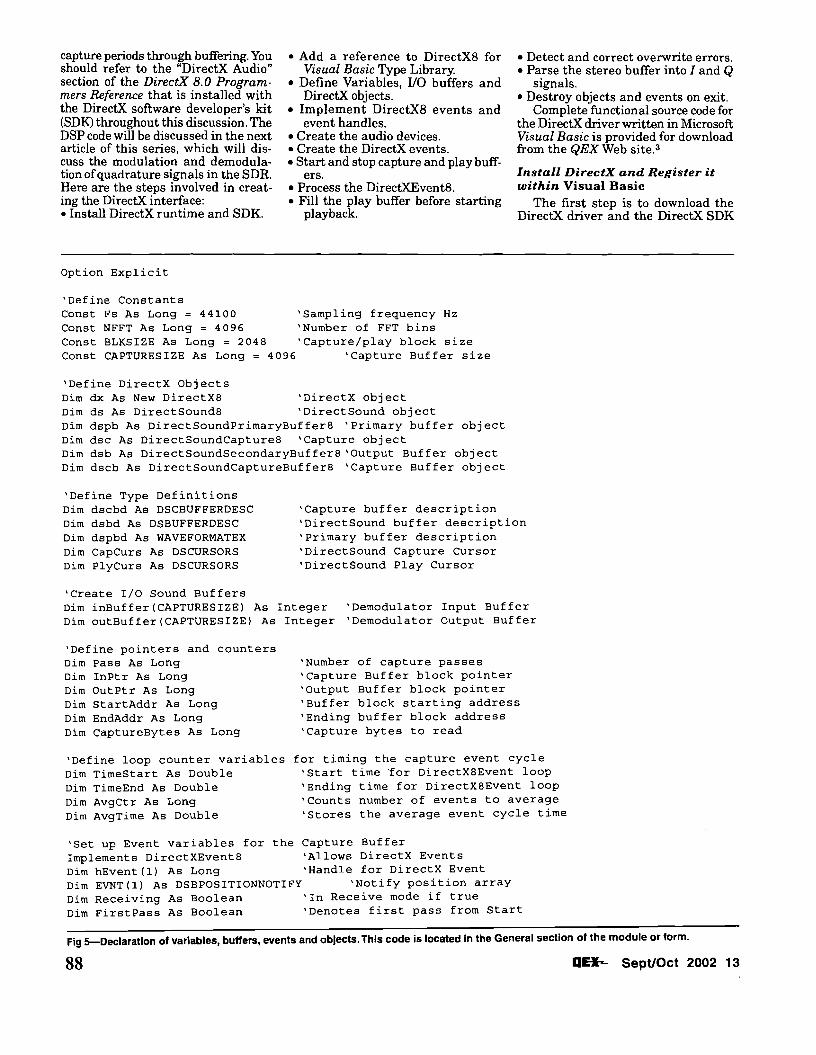
'Define loop counter variables for timing the capture event cycle Dim TimeStart As Double 'Start time £or DirectX8Event loop Dim TimeEnd As Double 'Ending time for DirectX8Event loop Dim AvgCtr As Long 'Counts number of events to average Dim AvgTime As Double 'Stores the average event cycle time
'Set up Event variables for the Capture Buffer Implements DirectXEvent8 'AllOWS DirectX Events Dim hEvent(l) As Long 'Handle for DirectX Event Dim EVNT(l) As DSBPOSITIONNOTIFY 'Notify position array Dim Receiving As Boolean 'In Receive mode if true Dim FirstPass As Boolean 'Denotes first pass from Start
Fig 5--Declaration of variables, bUffers, events and objects. This code is located in the General section of the module or form.
88 q~ Sept/Oct 2002 13

from the Microsoft Web site (see Note 3). Once the driver and SDK are installed, you will need to register the DirectX8 for Visual Basic Type Library within the Visual Basic development environment.
Ifyou are building the project from scratch, first create a Visual Basic project and name it "Sound."When the project loads, go to the Project Menu/ References, which loads the form shown in Fig 4. Scroll through Available References until you locate the
DirectX8 for Visual Basic Type Library and check the box. When you press "OK;' the library is registered.
Define Variables, Buffers and DirectX Objects
Name the form in the Sound project frmSound. In the General section of frmSound, you will need to declare all of the variables, buffers and DirectX objects that will be used in the driver interface. Fig 5 provides the code that is to be copied into the General sec
tion. All definitions are commented in the code and should be self-explanatory when viewed in conjunction with the subroutine code.
Create the Audio Devices We are now ready to create the
DirectSound objects and set up the format of the capture and play buffers. Refer to the source code in Fig 6 during the following discussion.
The first step is to create the DirectSound and DirectSoundCapture
'Set up the DirectSound Objects and the Capture and Play Buffers Sub CreateDevices()
On Local Error Resume Next
Set ds = dx.DirectSoundCreate(vbNullString) 'DirectSound object Set dsc = dx.DirectSoundCaptureCreate(vbNullString) 'DirectSound Capture
'Check to se if Sound Card is properly installed If Err.Number <> 0 Then
MsgBox "Unable to start DirectSound. Check proper sound card installation" End
End If
'Set the cooperative level to allow the Primary Buffer format to be set ds.SetCooperativeLevel Me.hWnd, DSSCL_PRIORITY
'Set up format for capture buffer With dscbd
With .fxFormat .nFormatTag = WAVE FORMAT PCM .nChannels = 2 'Stereo .lSamplesPerSec = Fs 'Sampling rate in Hz .nBitsPerSample = 16 '16 bit samples .nBlockAlign = .nBitsPerSample / B * .nChannels .lAvgBytesPerSec = .lSamplesPerSec * .nBlockAlign
End With .lFlags = DSCBCAPS_DEFAULT .lBufferBytes = (dscbd.fxFormat.nBlockAlign * CAPTURESIZE) 'Buffer Size CaptureBytes = .lBufferBytes \ 2 'Bytes for 1/2 of capture buffer
End With
Set dscb = dsc.CreateCaptureBuffer(dscbd) 'Create the capture buffer
, Set up format for secondary playback buffer With dsbd
.fxFormat = dscbd.fxFormat
.lBufferBytes = dscbd.lBufferBytes * 2 'Play is 2X Capture Buffer Size
.lFlags DSBCAPS_GLOBALFOCUS Or DSBCAPS GETCURRENTPOSITION2 End With
dspbd = dsbd.fxFormat 'Set Primary Buffer format dspb.SetFormat dspbd 'to same as Secondary Buffer
Set dsb = ds.CreateSoundBuffer(dsbd) 'Create the secondary buffer
End Sub
Fig 6-Create the DirectX capture and playback devices.
14 Sept/Oct 2002 q~ 89
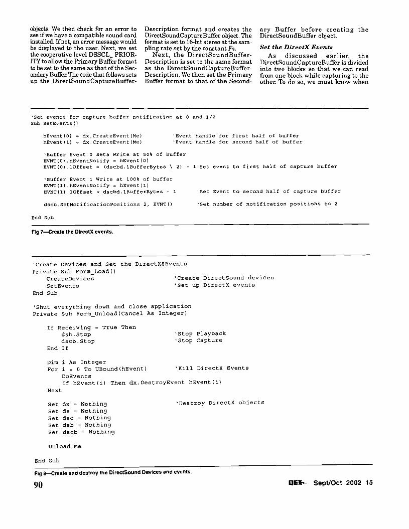
objects. We then check for an error to see if we have a compatible sound card installed. !fnot, an error message would be displayed to the user. Next, we set the cooperative level DSSCL_ PRIORITY to allow the Primary Buffer format to be set to the same as that of the Secondary Buffer. The code that follows sets up the DirectSoundCaptureBuffer-
Description format and creates the DirectSoundCaptureBuffer object. The format is set to 16-bit stereo at the sampling rate set by the constant Fs.
Next, the DirectSoundBufferDescription is set to the same format as the DirectSoundCaptureBufferDescription. We then set the Primary Buffer format to that of the Second
ary Buffer before creating the DirectSoundBuffer object.
Set the DirectX Events As discussed earlier, the
DirectSoundCaptureBuffer is divided into two blocks so that we can read from one block while capturing to the other. To do so, we must know when
'Set events for capture buffer notification at 0 and 1/2 Sub SetEvents ()
hEvent(O) dX.CreateEvent(Me) 'Event handle for first half of buffer hEvent(l) dx.CreateEvent(Me) 'Event handle for second half of buffer
'Buffer Event 0 sets Write at 50% of buffer EVNT(O) .hEventNotify = hEvent(O) EVNT(O) .lOffset = (dscbd.lBufferBytes \ 2) - l'Set event to first half of capture buffer
'Buffer Event 1 Write at 100% of buffer EVNT(l) .hEventNotify = hEvent(l) EVNT(l) .lOffset = dscbd.lBufferBytes - 1 'Set Event to second half of capture buffer
dscb.SetNotificationPositions 2, EVNT() 'Set number of notification positions to 2
End Sub
Fig 7-ereate the DlrectX events.
'Create Devices and Set the DirectX8Events Private Sub Form_Load()
CreateDevices 'Create DirectSound devices SetEvents 'Set up DirectX events
End Sub
'Shut everything down and close application Private Sub Form_unload(Cancel As Integer)
If Receiving = True Then dsb.Stop 'Stop playback dscb.Stop 'Stop Capture
End If
Dim i As Integer For i = 0 To UBound(hEvent) 'Kill DirectX Events
DoEvents If hEvent (i) Then dx.DestroyEvent hEvent(i)
Next
Set dx = Nothing 'Destroy DirectX objects Set ds = Nothing Set dsc = Nothing Set dsb = Nothing Set dscb = Nothing
Unload Me
End Sub
Fig 8--Create and destroy the DirectSound Devices and events.
QIE*s- Sept/Oct 2002 15 90

DirectX has finished writing to a block. This is accomplished using the DirectXEvent8. Fig 7 provides the code necessary to set up the two events that occur when the IWrite cursor has reached 50% and 100% of the DirectSoundCaptureBuffer.
We begin by creating the two event handles hEvent(O) and hEvent( 1). The code that follows creates a handle for each of the respective events and sets them to trigger after each half of the DirectSoundCaptureBuffer is filled. Finally, we set the number ofnotification positions to two and pass the name ofthe EVNTO event handle array to DirectX.
The CreateDevices and SetEvents subroutines should be called from the Form_LoadO subroutine. The Form_ Unload subroutine must stop capture and playback and destroy all of the DirectX objects before shutting down. The code for loading and unloading is shown in Fig 8.
Starting and Stopping Capture/Playback
Fig 9 illustrates how to start and stop the DirectSoundCaptureBuffer. The dscb.Start DSCBSTART_ LOOPING command starts the DirectSoundCaptureBuffer in a continuous circular loop. When it fills the first half of the buffer, it triggers the DirectX Event8 subroutine so that the data can be read, processed and sent to the DirectSoundBuffer. Note that the DirectSoundBufIer has not yet been started since we will quadruple buffer the output to prevent processor loading from causing gaps in the output. The FirstPass flag tells the event to start filling the DirectSoundBuffer for the first time before starting the buffer looping.
Processing the Direct-XEventB Once we have started the Direct
SoundCaptureBuffer looping, the completion ofeach block will cause the DirectX Event8 code in Fig 10 to be executed. Ai:, we have noted, the events will occur when 50% and 100% ofthe buffer has been filled with data. Since the buffer is circular, it will begin again at the 0 location when the buffer is full to start the cycle allover again. Given a sampling rate of 44,100 Hz and 2048 samples per capture block, the block rate is calculated to be 44,100/2048 = 21.53 blocks/s or one block every 46.4 ms. Since the quad buffer is filled before starting playback the total delay from input to output is 4 x 46.4 ms = 185.6 ms.
The DirectX Event8_DXCallback event passes the eventid as a variable.
the code determines from the eventid, which half of the DirectSoundCaptureBuffer has just been filled. With that information, we can calculate the start ing address for reading each block from the DirectSoundCaptureBuffer to the inBufferO array with the dscb. ReadBuffer command. Next, we simply pass the inBufferO to the external DSP subroutine, which returns the processed data in the outBufferO array.
Then we calculate the StartAddr and EndAddr for the next write location in the DirectSoundBuffer. Before writing to the buffer, we first check to make sure that we are not writing between the IWrite and IPlay cursors, which will cause portions ofthe buffer to be overwritten that have already been committed to the output. This will result in noise and distortion in the audio output. If an error occurs, the FirstPass flag is set to true and the pointers are reset to zero so that we flush the DirectSoundBuffer and start over. This effectively performs an automatic reset when the processor is overloaded, typically because ofgraphics intensive applications running alongside the SDR application.
If there are no overwrite errors, we write the outBufferO array that was returned from the DSP routine to the next StartAddr to EndAddr in the DirectSoundBuffer. Important note: In the sample code, the DSP subroutine call is commented out and the inBufferO array is passed directly to the DirectSoundBuffer for testing of the code. When the FirstPass flag is set to True, we capture and write four data blocks before starting playback looping with the .SetCurrentPosition o and .Play DSBPLAY_LOOPING commands.
The subroutine calls to StartTimer and StopTimer allow the average computational time ofthe event loop to be displayed in the immediate window. This is useful in measuring the effi
'Turn Capture/Playback On Private Sub cmdOn Click()
dscb.Start DSCBSTART_LOOPING Receiving True FirstPass = True
Start OutPtr = 0
End Sub
'Turn Capture/playback Off Private Sub cmdOff_Click()
Receiving False FirstPass = False dscb.Stop dsb.Stop
End Sub
ciency ofthe DSP subroutine code that is called from the event. In normal operation, these subroutine calls should be commented out.
Parsing the Stereo Buffer into I and Q Signals
One more step that is required to use the captured signal in the DSP subroutine is to separate or parse the left and right channel data into the I and Q signals, respectively. This can be accomplished using the code in Fig 11. In 16-bit stereo, the left and right channels are interleaved in the inBufferO and outBufferO. The code simply copies the alternating 16-bit integer values to the RealIn(», (same as 1) and ImagInO, (same as Q) buffers respectively. Now we are ready to perform the magic of digital signal processing that we will discuss in the next article ofthe series.
Testing the Driver
To test the driver, connect an audio generator--or any other audio device, such as a receiver-to the line input of the sound card. Be sure to mute linein on the mixer control panel so that you will not hear the audio directly through the operating system. You can open the mixer by double clicking on the speaker icon in the lower right corner of your Windows screen. It is also accessible through the Control Panel.
Now run the Sound application and press the On button. You should hear the audio playing through the driver. It will be delayed about 185 ms from the incoming audio because ofthe quadruple buffering. You can turn the mute control on the line-in mixer on and off to test the delay. It should sound like an echo. Ifso, you know that everything is operating properly.
Coming Up Next
In the next article, we will discuss in detail the DSP code that provides
'Start Capture Looping 'Set flag to receive mode 'This is the first pass after
'Starts writing to first buffer
'Reset Receiving flag 'Reset FirstPass flag 'Stop Capture Loop 'Stop Playback Loop
The case statement at the beginning of Fig 9-Start and stop the capture/playback buffers.
16 Sept/Oct 2002 q~ 91

'Process the Capture events, call DSP routines, and output to Secondary Play Buffer Private Sub DirectXEvent8 DXCallback (ByVal eventid As Long)
StartTimer 'Save loop start time
Select Case eventid 'Determine which Capture Block is readyCase hEvent(O)
Inptr = 0 'First half of Capture Buffer Case hEvent(l)
Inptr = I 'Second half of Capture Buffer End Select
StartAddr = Inptr * CaptureBytes 'Capture buffer starting address
'Read from DirectX circular Capture Buffer to inBuffer dscb.ReadBuffer StartAddr, CaptureBytes, inBuffer(O) , DSCBLOCK_DEFAULT
'DSP Modulation/Demodulation - NOTE: THIS IS WHERE THE DSP CODE IS CALLED DSP inBuffer, outBuffer
StartAddr = Outptr * CaptureBytes 'Play buffer starting address EndAddr = OutPtr + CaptureBytes - I 'Play buffer ending address
with dsb 'Reference DirectSoundBuffer
.GetCurrentPosition PlyCurs 'Get current Play position
'If true the write is overlapping the IWrite cursor due to processor loading If PlyCurs.IWrite >= StartAddr
And PlyCurs.IWrite <= EndAddr Then FirstPass = True 'Restart play buffer Outptr = 0 StartAddr = 0
End If
'If true the write is overlapping the IPlay cursor due to processor loading If PlyCurs.IPlay >= StartAddr _
And PlyCurs.IPlay <= EndAddr Then FirstPass = True 'Restart play buffer Outptr = 0 StartAddr = 0
End If
'Write outBuffer to DirectX circular Secondary Buffer. NOTE: writing inBuffer causes direct pass through. Replace
'with outBuffer below to when using DSP subroutine for modulation/demodulation .WriteBuffer StartAddr, CaptureBytes, inBuffer(O) , DSBLOCK_DEFAULT
Outptr = IIf(OutPtr >= 3, 0, Outptr + 1) 'Counts 0 to 3
If FirstPass = True Then 'On FirstPass wait 4 counts before starting Pass = Pass + 1 'the Secondary play buffer looping at 0 If Pass = 3 Then 'This puts the Play buffer three Capture cycles
FirstPass = False 'after the current one Pass = 0 'Reset the Pass counter .SetCurrentPosition 0 'Set playback position to zero .Play DSBPLAY LOOPING 'Start playback looping
End If End If
End With
StopTimer 'Display average loop time in immediate window
End Sub Fig 1O-Process the DirectXEvent8 event. Note that the example code passe~ t~e inBu!ferO directly to th~ D!rectSoundBuffer without processing. The DSP subroutine call has been commented out for this Illustration so that the ~udlo mput to the sound card will be passed directly to the audio output with a 185 ms delay. Destroy objects and events on eXIt.
92 qE*-o- Sept/Oct 2002 17
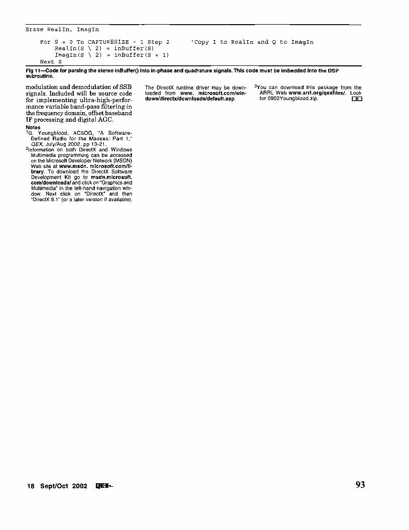
Erase Realln, Imagln
For 8 = 0 To CAPTURE8IZE - 1 8tep 2 'Copy I to Realln and Q to Imagln Realln (8 \ 2) inBuffer (8) Imagln(8 \ 2) = inBuffer(8 + 1)
Next 8
Fig 11-Code for parsing the stereo inBufferO into in-phase and quadrature signals. This code must be imbedded into the DSP subroutine.
modulation and demodulation of SSB signals. Included will be source code for implementing ultra-high-performance variable band-pass filtering in the frequency domain, offset baseband IF processing and digital AGe. Notes 'G. Youngblood, AC50G, "A Software
Defined Radio for the Masses: Part 1," OEX, July/Aug 2002, pp 13-21.
21nformation on both DirectX and Windows Multimedia programming can be accessed on the Microsoft Developer Network (MSDN) Web site at www.msdn.microsoft.com/library. To download the DirectX Software Development Kit go to msdn.microsoft. corn/downloads/ and click on "Graphics and Multimedia" in the left-hand navigation window. Next click on "DirectX" and then "DirectX 8.1" (or a later version if available).
The DirectX runtime driver may be down 3you can download this package from the loaded from www.microsoft.com/win ARRL Web www.arrl.org/qexfiles/. Look dows/directxldownloads/default.asp. for 0902Youngblood.zip. DO
18 Sept/Oct 2002 q~ 93


