
AD-A255 832
NSWCDD/TR-92/297
FIXED-GAIN, TWO-STAGE ESTIMATORS FOR
TRACKING MANEUVERING TARGETS
BY W.D. BLAIR
WEAPONS SYSTEMS DEPARTMENT
JULY 1992
Approved for public release; distribution is unlimited.
NAVAL SURFACE WARFARE CENTERr. DAHLGREN DIVISION
Dahigren, Virginia 22448-5000
19 DEFENSE TECHNICAL INFORMATION CENTER
9226238

NSWCDD/TR-92/297
FIXED-GAIN, TWO-STAGE ESTIMATORS FORTRACKING MANEUVERING TARGETS
BY W.D. BLAIRWEAPONS SYSTEMS DEPARTMENT
JULY 1992
Approved for public release; distribution is unlimited.
NAVAL SURFACE WARFARE CENTER
DAHLGREN DIVISIONDahigren, Virginia 22448-5000
V-io QUALT WRECT7I 3
NSWCDD/TR-92/297
FOREWORD
The classical problem of weapons control involves predicting the future position of a
maneuvering target. Critical to successful prediction is the accurate estimation of the current
target state. With the advent of guided weapons, the consequences of threat maneuver are
reduced when accurate estimates of the target state can be obtained. Threat trends indicate
that the conditions under vhi.i hostile targets can be engaged successfully are becoming
more difficult to achieve; hence, any improvement in existing estimation algorithms is of
critical importance.
This report presents the results of an investigation of an approach to the improvement
of an important class of target tracking algorithms. The work was supported by the Naval
Surface Warfare Center Dahlgren Division (NSWCDD) AEGIS Program Office.
This document has been reviewed by Dr. Richard D. Hilton of the Command Support
Systems Division and R. T. Lee, Head, Weapons Control Division.
Approved by:
DAVID S. MALYEVAC, Deputy Department Head
Weapons Systems Department

NSWCDD/TR-92/297
ABSTRACT
The two-stage Alpha-Beta-Gamma estimator is proposed as an alternative to adaptive
gain versions of the Alpha-Beta and Alpha-Beta-Gamma filters for tracking maneuveringtargets. The purpose of this report is to accomplish fixed-gain, variable dimension filtering
with a two-stage Alpha-Beta-Gamma estimator. The two-stage Alpha-Beta-Gamma estima-
tor is derived from the two-stage Kalman estimator, and the noise variance reduction matrix
and steady-state error covariance matrix are given as a function of the steady-state gains.
A procedure for filter parameter selection is also given along with a technique for maneuverresponse and a gain scheduling technique for initialization. The kinematic constraint for
constant speed targets is also incorporated into the two-stage estimator to form the two-
stage Alpha-Beta-Gamma-Lambda estimator. Simulation results are given for a comparison
of the performances of estimators with that of the Alpha-Beta-Gamma filter.
iii

NSWCDD/TR-92/297
CONTENTS
CHAPTER Page
1 INTRO D U CTIO N ............................................................ 1-1
2 STEADY-STATE KALMAN FILTERS ....................................... 2-1
ALPHA FILTER ........................................................... 2-2ALPHA-BETA FILTER .................................................... 2-4ALPHA-BETA-GAMMA FILTER ......................................... 2-6
3 TWO-STAGE KALMAN ESTIMATOR ...................................... 3-1
4 TWO-STAGE ALPHA-BETA-GAMMA ESTIMATOR ....................... 4-1
STEADY-STEADY RELATIONSHIPS ..................................... 4-3SELECTING GAMMA .................................................... 4-6MEASUREMENT VARIANCE REDUCTION MATRIX ................... 4-6INITIALIZATIO N ........................................................ 4-10EX A M PLE ............................................................... 4-13
5 TWO-STAGE ALPHA-BETA-GAMMA-LAMBDA ESTIMATOR ............. 5-1
6 SIMULATION RESULTS .................................................... 6-1
7 CONCLUSIONS AND FUTURE RESEARCH ................................ 7-1
R EFER EN C ES ..................................................................... 8-1
APPENDIXES
A DERIVATIONS FOR ALPHA-BETA FILTER ............................... A-1
STEADY-STEADY ERROR COVARIANCE AND GAINS ................ A-3MEASUREMENT VARIANCE REDUCTION MATRIX ................... A-4INITIALIZATION GAINS ................................................ A-6
B DERIVATIONS FOR ALPHA-BETA-GAMMA FILTER ..................... B-1
STEADY-STEADY ERROR COVARIANCE AND GAINS ................ B-3INITIALIZATION GAINS ................................................ B-5
D IST R IB U lIO N .................................................................... (1)
v

NSWCDD/TR-92/297
CHAPTER 1
INTRODUCTION
While the Kalman filter is known to produce an optimal estimate of the target state
when given the motion model and a sequence of sensor measurements corrupted with white
Gaussian errors, the computational burden of maintaining the Kalman filter may prohibit
its use when many targets are being tracked. A widely used approach to reducing the
computational burden of the filters involves the use of an approximate filter gain instead of
the optimal Kalman gain. The gain is usually based on the steady-state gains of the Kalman
filter and obtained by either using a fixed gain or an easily generated gain schedule. When
these steady-state or approximate gains are used, the resultant filters are called an a filter
for tracking position; an a, # filter for tracking position and velocity; and an a, /3,-y filter
tracking position, velocity, and acceleration.
For tracking systems with a uniform data rate and stationary measurement noise, non-
maneuvering targets can be accurately tracked with an a, # filter. However, when the target
maneuvers, the quality of the position and velocity estimates provided by the filter can de-
grade significantly, and for a target undergoing a large maneuver, the target track may be
lost. An a, fl, y filter can be used to track such a target, but the accelerations of a maneuver-
ing target are seldom constant in the tracking frame during the maneuver. If the a gain of
the a, /, -y filter is chosen small to achieve good noise reduction, the "optimal" -Y of Kalata [1]
will be very small and the acceleration estimates will respond slowly to a maneuver. Thus,
in order for the a, #, y- filter to respond quickly to a maneuver, a must be maintained at a
high level and the filter will provide poor noise reduction (noisy estimates) when the target
is not manuevering. The noisy target state estimates may hinder the sensor pointing, data
association, and other control decisions and computations based on the state estimates.
One approach to overcoming this filtering dilemma is to use a small a until a maneuvcr
is detected. Then a is increased for tracking through the maneuver. This approach was
investigated by Cantrell [2] and Blackman [3]. It has two major problems. First, the response
1-1

NSWCDD/TR-92/297
of the filter is significantly delayed because the gains are not increased until a maneuver is
detected. Furthermore, in the a, /3 filter, the a gain must be set artificially high to account
for the absence of acceleration from the motion model. Second, after a target has returned
to constant velocity from a maneuver, the decision to reduce a is often delayed because there
is no bias in the higher gain a,/3.filter to detect.
An alternate approach, which seems to be attractive, is to continuously estimate the
target acceleration and correct the position and velocity estimates of the a, /3 filter whenever
a maneuver is detected. The purpose of this report is to accomplish fixed-gain, variable
dimension filtering with a two-stage a, /3, ' estimator, as suggested by Alouani et. al. [4,51
for the two-stage Kalman estimator. In the two-stage a,/3, # estimator, position and velocity
are tracked in the first stage, which is a standard a, /3 filter, and the acceleration is tracked in
the second stage, which is a standard single gain filter. The output of the acceleration filter
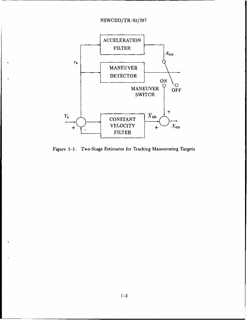
can be used to adjust the estimates of the a,/3 filter, as shown in Figure 1-1 when a bias is
detected. This approach to tracking maneuvering targets is similar to input estimation in
[6-81, with the exception that the acceleration is modeled as a stochastic process instead of
a deterministic process as in input estimation. The two-stage estimator has the good noise
reduction associated with the a, /3 filter when the target is not maneuvering, and when a
maneuver is detected, an acceleration estimate is available to compensate the estimates of
the a, /3 filter. Furthermore, since the acceleration is not part of the central filter, the ' gain
can be picked somewhat independent of a to improve maneuver response.
When targets maneuver while maintaining a constant speed, the accelerations vary with
time throughout the maneuver and the estimates of both the a, /3, Y filter and the two-stage
a,/3, ý estimator will be biased. The kinematic constraint for constant speed targets can
be included as a pseudomeasurement in the filtering process to reduce the filter bias as in
[9]. The kinematic constraint for constant speed targets is incorporated into the two-stage
estimator to form the two-stage a, /3, 7, A estimator.
This report is organized as follows. In Chapter 2, steady-state Kalman filters are dis-
cussed, and the a, /3 filter and a, /3, -y filter are summarized. The two-stage Kalman estimator
is presented in Chapter 3. In Chapter 4, the two-stage a, /3, 1 estimator is derived, and proce-
dures for gain selection during initialization and steady-state conditions are presented along
with the concept of a soft switch for maneuver response. The two-stage a, /3, ', A estimator
is presented in Chapter 5. Simulation results for a radar tracking system are presented in
Chapter 6 for the two-stage estimators and the a, /3, -y filter. Some concluding remarks are
given in Chapter 7 along with a discussion of future research.
1-2
NSWCDD/TR-92/297
ACCELERATION
FILTER Al
rk
MANEUVER
DETECTOR_____ ____ON \
MANEUVER OFFSWITCH
YIC ~CONSTANT X~
+ VELOCITY + XklkFILTER
Figure 1-1. Two-Stage Estimator for Tracking Maneuvering Targets
1-3

NSWCDD/TR-92/297
CHAPTER 2
STEADY-STATE KALMAN FILTERS
A Kalman filter is often employed to filter the position measurements for estimating the
position, velocity, and/or acceleration of a target. When the target motion and measurement
models are linear and the measurement and motion modeling error processes are Gaussian,
the Kalman filter provides the minimum mean-square error estimate of the target state.
When the target motion and measurement models are linear, but the noise processes are not
Gaussian, the Kalman filter is the best linear estimator of the target state in the mean-square
error sense. The dynamics model commonly assumed for a target in track is given by
Xk+1 = FkXk + Gkwk (2.1)
where wk - N(O, Qk) is the process noise and Fk defines a linear constraint on the dynamics.
The target state vector Xk contains the position, velocity, and acceleration of the target at
time k, as well as other variables used to model the time-varying acceleration. The linear
measurement model is given by
Yk = HkXk + nk (2.2)
where Yk is usually the target position measurement and nk - N(O, Rk). The Kalman
filtering equations associated with the state model in Eq. (2.1) and the measurement model
in Eq. (2.2) are given by the following equations.
Time Update:
Xkjk-1 = Fk-mXk-ljk-1 (2.3)
Pkjk-1 = Fk-1Pk-Il k-lFT-I + k-lQk-IG Tm(2.4)
Measurement Update:
Kk = PklkIaHk [HkPklk-aHk + Rk]- (2.5)
Xkjk = Xk 1k- 1 + Kk[Yk - HkXklk-1] (2.6)
Pkjk = [I-- KHk]Pklk-I (2.7)
2-1

NS'.VCDD/TR-92/297
where Xk - N(Xklk, Pkjk) with Xkjk and Pkjk denoting the mean and error covariance of the
state estimate, respectively. The subscript notation (klj) denotes the state estimate for time
k when given measurements through time j, and Kk denotes the Kalman gain. Using the
matrix inversion lemma of [10] and Eqs. (2.5) and (2.7), an alternate form of the Kalman
gain is given by
H= Pkjk-j H[HkPk 1k-4HT + R-11-1= [I- PkjlkHTRj 1 1k1 -1PkIkiHTR-1
=1- PkIk_.Hr(HkPklkIHk + R-I)-IHk]Pklk_,kItR-j
[I KkHk]Pklk 4 HjR-'
= PkIkHTR- 1 (2.8)
The steady-state form of the Kalman filter is often used in order to reduce the computa-
tions required to maintain each track. In steady-state, Pkjk = Pk-ilk-1, and Pk+ lk = Pklk-1,
and Kk = Kk-1. For a Kalman filter to achieve these steady-state conditions, the error pro-
cesses, wk and nk, must have stationary statistics and the data rate must be constant.
When the noise processes are not stationary or the data rate is not constant, a filter using
the steady-state gains will provide suboptimal estimates. The a, 3 and a,'3, -Y filters are the
steady-state Kalman filters for tracking nearly constant velocity targets and nearly constant
acceleration targets, respectively. First, the a filter for tracking nearly constant position
targets will be considered. Then the a, 0 and a, /3, filters will be considered.
ALPHA FILTER
The a filter is a single coordinate filter that is based on the assumption that the tar-
get position is constant plus zero-mean, white Gaussian acceleration errors. Given this
assumption, the filter gain a is chosen as the steady-state Kalman gain that minimize the
mean-square error in the position estimates. For the a filter,
Xk = [Xk ]T (2.9)
Fk = [11 (2.10)
Gk = T2 ] (2.11)
Hk =[11 (2.12)
Rk = o' (2.13)
Qk = oW2 (2.14)
2-2

NSWCDD/TR-92/297
Kk = [a]T (2.15)
The steady-state error covariance of the filtered estimates for the a filter can be expressed
as a function the Kalman gain using Eq. (2.8) to be
Pk+llk+l = Pklk = P = an 2 (2.16)
Using Eq. (2.4) in Eq. (2.7) and inse:ting Eq. (2.16) for P gives
T4a = [1- a][aO + T 2 1 (2.17)
Thus, Eq. (2.17) gives
2 T4,2 4a 2T ,- 4a(2.18)V0 1- a
where r is the Tracking Index of [11], and a,2 is the variance of the acceleration modeling
error. Thus, the a gain is determined as in [11 from r by solving the Eq. (2.18). Note the
these steady-state relationships result from the assumption that the model error process is
acceleration errors that are constant through each measurement sample period.
The input-output relationships between the measurements Yk and Xk1 k can be expressed
as a linear system that is given by
Xk1k = (1 - a)Xk-Ilk-1 + ayk (2.19)
Using Eq. (2.19) provides the error covariance of Xklk that results from the measurement
errors. Let Yk be a white noise stationary sequence with zero mean. Then E[XkXk] = k=
Sk-1 = S,, which is given by- _ oaSo(- 2' (2.20)
2-2The variance reduction ratio of the filter is given by Eq. (2.20) when au = 1.
Since during initialization the a filter is not in a steady-state condition, Eq. (2.16) cannot
be used to determine a. Using least-squares estimation in conjunction with a constant state
model, a simple gain scheduling procedure for a during initialization is given by
ak = Max{(k 1 (2.21)
with Xo1_1 = [0 1T. The derivation of Eq. (2.21) follows closely the derivation for the gains
for initializing the a, 0 filter in Appendix A.
2-3

NSWCDD/T R-92/297
ALPHA-BETA FILTER
The a,,3 filter is a single coordinate filter that is based on the assumption that the target
is moving with constant velocity plus zero-mean, white Gaussian acceleration errors. Given
this assumption, the filter gains a and 3 are chosen as the steady-state Kalman gains that
minimize the mean-square error in thc position and velocity estimates. For the a, 13 filter,
Xk = [xk ikIT (2.22)
Gk= [ T] (2.24)
Hk = [1 01 (2.25)
Rk = Orv (2.2-,)
Qk = aOw (2.27)
Kk== a (2.28)
The a, 13 gains are determined as in [1,3,8] by solving the simultaneous equations
rF2 = T _4 w 13 (2.29)
3 = 2(2 - a) - 4v'1 -a (2.30)
where ow2 is ._e vwiance of the acceleration modeling error.
The steady-state error covariance of the filtered estimates for the a, 3 filter is given in
[1,81 as
0,2 T (2.31)
T 2(1 - a)T 2
The steady-state gains and error covariance in Eqs. (2.29) through (2.31) are derived in
Appendix A. Note that theie steady-state relationships result from the assumption that
the model error prrcess is acceleration errors that are constant through each measurement
sample pcric'.
In target tracking, a conflict arises between the goals of good noise reduction which
requires small a (and thus, small 13), and good tracking through maneuvers which requires
a larger a. For good noise reduction, heavy filtering is used and a filter with slow system
2-4
NSWCDD/TR-92/297
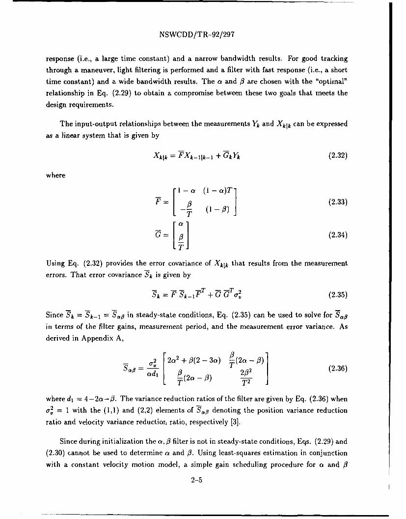
response (i.e., a large time constant) and a narrow bandwidth results. For good tracking
through a maneuver, light filtering is performed and a filter with fast response (i.e., a short
time constant) and a wide bandwidth results. The a and # are chosen with the "optimal"
relationship in Eq. (2.29) to obtain a compromise between these two goals that meets the
design requirements.
The input-output relationships between the measurements Yk and Xklk can be expressed
as a linear system that is given by
Xklk = FXk-Ilk-l + GkYk (2.32)
where
F = - (2.33)T
G = •(2.34)
Using Eq. (2.32) provides the error covariance of Xk1 k that results from the measurement
errors. That error covariance Sk is given by
Sk = F Skl-fT - v (2.35)
Since Sk = Sk-1 = S,6 in steady-state conditions, Eq. (2.35) can be used to solve for Saf
in terms of the filter gains, measurement period, and the measurement error variance. As
derived in Appendix A,
0,.2 12a2±+#(2 -- 3a) ý(2a -~(.6ad2 (2a-,3)2 (2236)
where di = 4- 2a -0. The variance reduction ratios of the filter are given by Eq. (2.36) when2 = 1 with the (1,1) and (2,2) elements. of S3f denoting the position variance reduction
av
ratio and velocity variance reductior, ratio, respectively [3].
Since during initialization the a, 1 filter is not in steady-state conditions, Eqs. (2.29) and
(2.30) cannot be used to determine a and 13. Using least-squares estimation in conjunction
with a constant velocity motion model, a simple gain scheduling procedure for a and 13
2-5
NSWCDD/TR-92/297
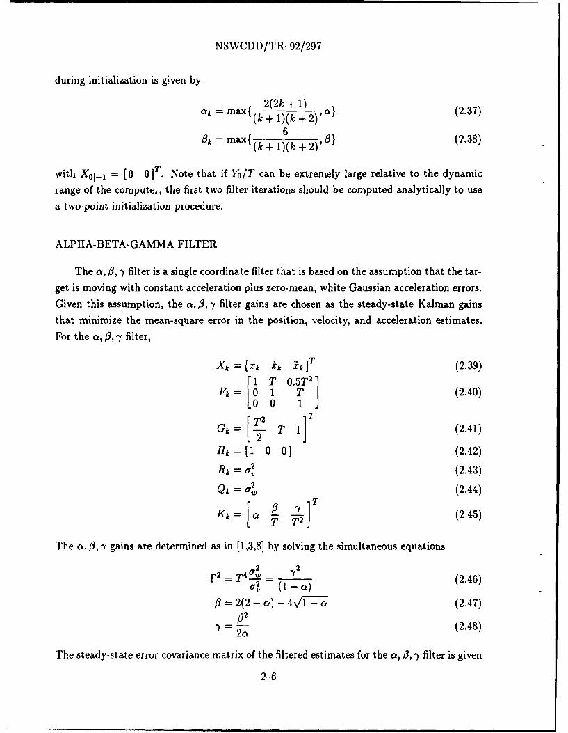
during initialization is given by
2(2k + 1)ak = maxi (k + 1)(k + 2)a} (2.37)
max{ (k + 1)(k + 2)'/Il (2.38)
with X01_1 = [0 0 iT. Note that if Yo/T can be extremely large relative to the dynamic
range of the compute., the first two filter iterations should be computed analytically to use
a two-point initialization procedure.
ALPHA-BETA-GAMMA FILTER
The a, #, -y filter is a single coordinate filter that is based on the assumption that the tar-
get is moving with constant acceleration plus zero-mean, white Gaussian acceleration errors.
Given this assumption, the a, #, -1 filter gains are chosen as the steady-state Kalman gainsthat minimize the mean-square error in the position, velocity, and acceleration estimates.
For the a, -,y filter,
Xk= [xk ik -k IT (2.39)
[1T 0.5T 2 ](40
Gk= T2 T ]T (2.41)
Hk =[1 0 0] (2.42)
Rk = av (2.43)
Qk = aw (2.44)
S= , L(2.45)
The a, -,t• gains are determined as in [1,3,81 by solving the simultaneous equations
o2 2F 2 =T 4 aWr2 (1-0) (2.46)
/= 2(2- a) V14V - a (2.47)Y = (2.48)
2ai
The steady-state error covariance matrix of the filtered estimates for the a, /, 1 filter is given
2-6

NSWCDD/TR-92/297
in [1,81 as
a TT
Pk 2 I= 4a,3+ -t-(P - 2a - 4) 3(,3 - -y) (2.49)P =a 4(1 - a)T 2 2(1 - a)T 3
T2 2(1 -a)T 3 (1 -a)T 4
The steady-state gains and error covariance in Eqs. (2.46) through (2.49) are derived in
Appendix B.
The input-output relationships between the measurements Yk and filtered state Xktk can
be expressed as a linear system that is given by
1 -a (1 -a)T (1- a)--2 a
/3 (1 x + ] Yk (2.50)
T 2"7 -7 1 - L72
Using Eq. (2.50) provides the steady-state error covariance of Xklk that results from the
measurement errors. That error covariance S3,f as given in [11] is
\did2/
2ad2 -2(6a - 4) + a/3y (2a - )(2/ - --) T2-(2d 2 + 0(-y - 20))(2- )(2- 7) --2(72(2 - a) + 2#2(p _- 7)) 2T( ).
~((2 V~-(/ (2.51)2/3• 4/37 2
- (2d2 + 0(-y - 20)) -1 (20-7)L TiV
where dI = 4 - 2a - # and d2 = 2a# + -y(a - 2). The measurement error variance reduction
ratios of the filter are given by Eq. (2.51) when o2 = 1 with the (1,1), (2,2), and (3,3)
elements of Sa.- denoting the position variance reduction ratio, velocity variance reduction
ratio, and the acceleration variance reduction ratio, respectively.
Using least-squares estimation in conjunction with a constant acceleration motion model,
a simple gain scheduling procedure for a, / and 7 during initialization is given byak = max( 3(3k2 + 3k + 2) ,al (2.52)
(k + 1)(k + 2)(k + 3)
=max{ 18(2k + 1) , 0} (2.53)8k max(k•" + 1)(k + 2)(k + 3)
7k = max{k ,03 7} (2.54)+ 1)(k + 2)(k + 3)
2-7

NSWCDD/TR-92/297
with X01-1 = [0 0 0 ]T. Note that if Y0,1/T 2 can be extremely large relative to the
dynamic range of the computer, the first three iterations of the filter should be computed
analytically to use a three-point initialization procedure.
2-8

NSWCDD/TR-92/297
CHAPTER 3
TWO-STAGE KALMAN ESTIMATOR
Consider the problem of estimating the state of a linear system in the presence of a
random bias that influences the system dynamics and/or observations. The bias vector may
represent a part of the augmented system state as suggested in [12]. The idea of using a
two-stage filter to implement an augmented state filter was introduced in [12]. The idea is
to decouple the central filter into two parallel filters. The first filter, the "bias-free" filter,
is based on the assumption that the bias is nonexistent. The second filter, the bias filter,
produces an estimate of the bias vector. The output of the first filter is then corrected
with the output of the second filter. It was shown in [12] that if the bias is deterministic
and constant, but unknown, the two-stage filter is equivalent to the augmented state filter.
It was shown in [4,13] that under an algebraic constraint on the correlation between the
state process noise and the bias process noise, the proposed two-stage Kalman estimator is
equivalent to the augmented state Kalman filter.
Consider a linear system whose dynamics is modeled by
Xk+j = FkXk + Gkbk + GXWX (3.1)bk+1 = bk + GW' (3.2)
where Xk is an n dimensional system state vector, bk is a p dimensional bias vector. This
system may represent the dynamics of a maneuvering target, where the position and velocity
are the system state and the bias represents the target acceleration. The WX and Wb are
white Gaussian sequences with zero means and variances given byE[W (wX) T ] - Q•,kl (3.3)
E[Wb(wb) T] b Qb6k (3.4)
E[Wx(WP)T] = QTXb , (3.5)
The state measurement model at time k is given byYk = HkXk + Ckbk + vk (3.6)
3-1

NSWCDD/TR-92/297
where Yk is the measurement and vk - N(O, Rk) is the measurement error. The standard
approach to estimating the state and bias is to form an augmented state model which includes
both the bias and the state. With this augmented state model, a Kalman filter may be used
to produce the optimal state estimates.
If the bias term is ignored, (bk = 0), the bias-free filter is the Kalman filter based on the-xmodel in Eqs. (3.1) and (3.6), where fictitious statistics are used for Wx (i.e., Qk is used
instead of G Qj (GX)T). The bias-free filter is given by
Xkjk- 1 = Fk-.1X`-1t,-1 (3.7)_x
Xkjk = Xkjk-1 + Kk [ _ - 1 kXklk-11 (3.8)x -x T x
Pkk-i = FklPk- 1 klF7Il + Qk-_ (3.9)-X -X -xPkjk = (I - Kk Hk)PFkl,1k- (3.10)-yX =_---Xk_ T -X fT -
PklkjA; [HPlk,_lHkT + Rkd- (3.11)--X
where Qk-U is defined later in this chapter. The k- Xkjk represents the estimate of the state
process when the bias is ignored, and Pklt, is the error covariance of Xklk.
As in [121, a separate filter may be used to estimate the bias vector from the residual
sequence of the bias-free filter. The bias filter is given by
bkk-1 = bk.-llk-1 (3.12)bklk = bkjk-1 + K'[r, - Skbkjkt.l] (3.13)
Pbl, Pb lb l b _ )TPk-k-1 = Il-I + G' -(G (3.14)
K• b p T Skb sT X Tk _k [S-iPk k`_I1T + Hk kik-_lHT + Rd]- (3.15)
Pb -bI - KkSk)P•,ltI_ (3.16)
where
Sk= HUk + Ck (3.17)
Uk = Fk_, Vk_1 + Gk.•1 (3.18)vt ( -x 7xc 3.)
Vk= (I-Kk Hk)Uk -KkCk (3.19)
and rk is the residual of the bias-free filter. Initialization of this bias filter is discussed later
in this chapter.
The algorithm for compensating the output of the bias-free filter with the output of the
bias filter is given by
Xkik = E[XS] = Xkjk + Vkbklk (3.20)
3-2
NSWCDD/TR-92/297
Pkjk = E[(Xk - Xklk)(Xa - Xkak) T ] = Pk_ + VkPkV[ (3.21)Pflkb = EI(Xk - Xklk)(bk - bklk)T] = VkPkIk (3.22)
P bk = E[(bk - bklk)(bk - bklk)] = Pkbj (3.23)
The structure of the two-stage Kalman estimator is shown in Figure 3-1.
Theorem: IfGXQXbb(Gb)T Uk+G bQb (Gb )T (3.24)
k •€k k-a k-a- k, • k}
-Xand the error covariance Qx of the process noise of the bias-free filter model given by_- XT XX b b b TukT
Qk = GkQk(GX) - Vk+lGaQa(G ) V.,+, (3.25)
is positive semidefinite, then the filter given by Eqs. (3.20)-(3.23) is equivalent to the aug-
mented state filter.
Proof: See [4,13].
While the algebraic constraint of Eq. (3.24) will not be .2atisfied by almost all real
systems, the theorem provides a basis for assessing the degree of suboptimality of a two-
stage estimator when applied to specific problems. For example, let the algebraic constraint
of Eq. (3.24) be expressed as
- (G -a < + )U+GQ(G) T k > 0 (3.26)
Then for a given system, the smallest positive e that satisfies Eq. (3.26) indicates the degree
of suboptimality of the two-stage estimate with respect to the augmented state filter.
For initialization of the two-stage estimator, PXb = 0 if the initial estimate of the bias010is uncorrelated with the initial estimate of the bias-free state. If PXb = 0 Eqs. (3.22) and010(3.19) imply that V0 = 0 and UO = 0. Note that as shown in [4,13] the initialization does
not require PXb = O.
For the system and bias models given in Eqs. (3.1) and (3.2), the process noise covari-
ances are given in Eqs. (3.3) through (3.5). However, for tracking targets with the two-stage
estimator, the process noise covariances in Eqs. (3.3) through (3.5) are design parameters.
When designing the two-stage estimator for tracking maneuvering targets, Qk can be chosen
to obtain the desired response of the constant velocity filter and Qb can be chosen for ma--- X
neuver response. In this type of design procedure, Qk is chosen to be positive semi-definite
and Qx is allowed be a free parameter that depends on the selection of _x and Qb.
3-3

NSWCDD/TR-92/297
+
I-- KkSEk DELAY•
............ ............ ............................ ........................................................ .
bkl
r................................. ----------............................. •...........................
kk~Yk _kj
SDELAY
BIAS-FREE FILTER
Figure 3-1. Structure of Two-Stage Kalman Estimator
3-4

NSWCDD/TR-92/297
CHAPTER 4
TWO-STAGE ALPHA-BETA-GAMMA ESTIMATOR
For a uniform data rate and stationary noise processes, the single coordinate version
of the two-stage Kalman estimator can be approximated with a filter including three fixed
gains. In this fixed-gain filter, the two-stage a, P3, I estimator, the position and velocity are
tracked in the first stage, which is a standard a, #3 filter, and the acceleration is tracked
separately in the second stage, which is a standard single gain filter. The output of the
acceleration filter can be used to adjust the estimates of the a, fl filter, as shown in Figure
4-1, when a maneuver is detected. The parameters K1 , K2 , and 1K3 will be defined later.
The bias-free filter of Eqs. (3.7)-(3.11) corresponds to the standard constant velocity
filter in a single coordinate when
Fk=[I aT] (4.1)_-X
Qk = q--Lk(4.2)
Gk = Gx= TI T (4.3)
Hk=[1 0], Ck= 0 (4.4)
TX = ýk TKk ak (4.5)
for scalar acceleration error variance /. The bias filter of Eqs. (3.12)-(3.16) corresponds
to the standard constant state filter with residuals of the bias-free filter, rk, as the input
and G1 = 1. Since the bias corresponds to a scalar acceleration, the bias filter gain will be
a scalar. Let the bias filter gain be denoted as
-- -S , k > 0 (4.6)
where lk are Sk are positive scalars obtained from Eqs. (3.15) and (3.17). Letting bk = Ak
and inserting Eq. (4.6) into Eq. (3.13) gives
Aklk = AkIk-1 + 7k[Sk-Irk - AIk.-l] (4.7)
4-1

NSWCDD/TR-92/297
iKIT +(
ACCELERATION FILTER
SWITCH
1 T+IE0 1 ,CONSTANT VELOCITY FILTER
Figure 4-1. Two-Stage a,# fl, Estimator
4-2

NSWCDD/TR-92/297
Using Eqs. (4.1) through (4.7) in the bias-free and bias filters gives the two-stage a,#,
estimator as summarized by the following equations:
Prediction
"Xkjk-1 = Fk.-1Xk- 1k- 1 (4.8)
Akljk_j = Ak-llk_1 (4.9)
1a-1 A3 -1 T
Uk = A-1 UI+ Gk- (4.10)
T1
Measurement Update
Xkjk = Xkjk-a + Kk(y - H:X 1y.a) (4.11)
Aklt = (1 - k)Akjkl +IUSkirk (4.12)
Output Correction
Xkjk = Xkjk + VkAklk (4.13)
Vk[Ik l]Uk (4.14)ST
where the gains are a function of time. In steady-state conditions, ak = a, lk = /3, and
7k = -. Also, the bias filter is initialized with A01- 1 = 0 and U- 1 = [0 0 ]T.
STEADY-STATE RELATIONSHIPS
If the measurement rate is uniform (i.e., T is constant), the measurement error statisticsare stationary (i.e., R, = oa2), and the acceleration error statistics are stationary (i.e., '=
&.,), then the bias-free filter in steady-state conditions corresponds to an a, /3 filter with
ak = a and /3k = 3. Then a and / are given by Eqs. (2.29) and (2.30) for the a, /3 as-2 #2
-=T4 I-2 (4.15)
3 = 2(2 - a) 4Vi -- a (4.16)
where V' denotes the tracking index for the bias-free filter.
Since the statistics of the residuals rk in the a, /3 filter will be stationary in steady state,
the bias filter will achieve steady-state conditions if the statistics of Wkb are stationary (i.e.,
Qb= a2). The bias filter in steady-state conditions corresponds to a single gain filter with
Kb = Kb = ýS-l (4.17)
4-3
NSV; CDD/TR-92/297
Qb = a2 ). The bias filter in steady-state conditions corresponds to a single gain filter with
K6 = K=b S (4.17)
where S is a constant scalar in steady-state conditions. Using Eqs. (4.10) and (4.14), the
steady-state parameters are
Uk+l = Uk = U = (T + 0.5)T] (4.18)I #oVk+ = V = V = -)-O.T2 I
The steady state values of K 1, K2, and K 3 in Figure 4-1 are given by
K1 = S-1 = (HkU)- 1 T (4.20)
[KK2]=V (4.21)
Since the two-stage a, 3, 5• estimator is an a, /3 filter when the switch is open, the steady-
state error covariance Pkk =P is provided by Eq. (2.31) as
-- X -. X 2 a T (4.22)Pklk = P = Ov /3 0(2a - 0)
T 2(l - a)T2
The variance of the residuals of the bias-free or a, 3 filter is given by
2 -T X T T +2(4.2aURES = Hk FkPi Fki Hk + qkHkGkGGk Hk + (4.23)
Inserting Eqs. (4.1) through (4.4) and (4.22) into Eq. (4.23) gives
2 2[1 a +3(3 - ) TV 22=(1 + +T& . (4.24)a2RS =aS[ + +2(l - ] a) 4
Using Eq. (4.15) to eliminate &2 from Eq. (4.24) and using a 2 - 2/3 + a/3 + 0.25/3 = 0 of [8]
gives
2 _ a2aaRES - (4.25)
S-(1 -
Thus, using Eq. (4.25) in conjunction with Eq. (4.20) gives the variance of the input to the
second stage or bias filter as (KI) 2a3RES. Using Eqs. (2.8) and (4.15) gives the steady-state
gain for the second stage as
pb ( -2 -1 Pb( /32 2 = ,'(T4( ) pb&W2 (4.26)
4-4
NSWCDD/TR-92/297
Thus, the steady-state error covariance of the second stage is given by
pb = 1 ( "' ) 2 -- 2 (4.27)
Inserting Eq. (2.4) into Eq. (2.7) for the bias filter givespb = l-q]pl + 0,2,!(.8
p6 [1~[P+. 2 (4.28)
Thuspb(1-) 2 (4.29)
Eqs. (4.27) and (4.29) giveW - (4.30)
S(1
Using Eqs. (4.19) and (4.27) in Eq. (3.22) gives
pXb =pXb - Vpb 2 T2 (4.31)k~k -a (ab 0.0v
(1 a)T 3
Using Eqs. (4.19) and (4.31) gives
a (a -0.513)1VPbVT -2 T
(a - 0.513) (a - 0.503)2 (4.32)
T (I - a)T 2
Since the output error covariance of the two-stage estimator is dependent on the maneuver
switch, let the switch gain be denoted by
(0, switch openGs = (4.33)
', switch closed
Using Eqs. (4.22), (4.27), (4.31), and (4.32) in Eqs. (3.21) through (3.23) gives the output
error covariance of the two-stage estinmator as a function of the maneuver switch to be
Pklk(1, 1) -= a24) s,-[(a + (1 - a)Gs) (4.34)
0.2,Pkk(1,2) = -#[0 + (a - 0-50)Gs] (4.35)
Pklk(1, 3 ) = a,213 (4.36)Pklk(2,2) = a 0 ( .51 3)11 5 + (a - 0.50)Gs] (4.37)
2 (1 - 05)T2
Pkjk( 2 , 3 ) = 0,, (1 -_ 0 a s (4.38)
1)32
Pklk(3,3) = a )T4 Gs (4.39)
4-5

NSWCDD/TR-92/297
where Pklk(i,J) denotes the (i,j) element of the error covariance.
SELECTING GAMMA
Since the algebraic constraint of Eq. (3.24) will not be satisfied, the two-stage estimator
with the maneuver switch closed will not be identical to the augmented state filter (i.e.,
the a, 3, -/ filter). However, the position, velocity, or acceleration variances of the two-stage
estimator and the a, ,3,y filter can be matched through the selection of Y. Using the (1,I)
elements of Eqs. (2.49) and (4.34), a match between the position variances is given by
a-a (4.40)(1 -a)
where & denotes the alpha gain of a standard a, /, y filter that is desired for tracking through
maneuvers. Using the (2,2) elements of Eqs. (2.49) and (4.37), a match between the velocity
variances is given by
+[ - ( +0.25Y(/- 2& - 4)) (4.41)= .(1-----• B (-a -- 0.5# )2 0 .50• 4.1
where &, /, j denote the gains of a standard a, /#, -1 filter that is desired for tracking through
maneuvers. Using the (3,3) element of Eq. (2.49) and Eq. (4.39) gives a match between the
acceleration variances as
/32ji.[I.-a] (4.42)
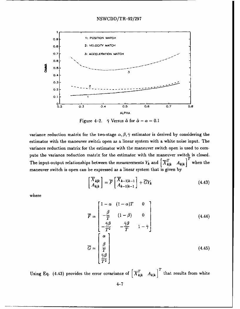
Fig. 4-2 gives various values of , versua& & for matching the position, velocity, or accel-
eration variances when & - a = 0.1. Using Fig. 4-2, consider the two-stage estimator with
a = 0.3 and ' = 0.2 and the a, /, y filter with & = 0.4. Then the position and velocity esti-
mates of the two-stage estimator with the maneuver switch closed will closely match those
estimates of the corresponding a, i, y filter, while the acceleration estimates of the two-stage
estimator will be filtered more heavily than those of the a, /, -y filter. Fig. 4-2 also shows
that the estimates of two-stage estimator for & - a = 0.1 will more closely match those of
the augmented state filter, the a, /,7 filter, when 0.4 < a < 0.5 and 0.25 <_ <0.5.
MEASUREMENT VARIANCE REDUCTION MATRIX
The variance reductions between position, velocity, and acceleration estimates and the
measurements are often considered in the design and analysis of fixed-gain filters. The
4-6
NSWCDD/TR-92/297
0.9 1: POSITION MATCH
0.8 2: VELOCITY MATCH
0.7 3: ACCELERATION MATCH.. -
0.6'
0.5 -" -
0.4
0.3-
0.2 .....................
0.1
0[0.2 0.3 0.4 0.5 0.6 0 7 0.8
ALPHA
Figure 4-2. ý Versus & for a - a = 0.1
variance reduction matrix for the two-stage a, #,,;y estimator is derived by considering the
estimator with the maneuver switch open as a linear system with a white noise input. The
variance reduction matrix for the estimator with the maneuver switch open is used to com-
pute the variance reduction matrix for the estimator with the maneuver switch is closed.
The input-output relationships between the measurements YI and T Aklk when the
maneuver switch is open can be expressed as a linear system that is given by
klk L [Ak-llk-1 + GYk (4.43)
where
"1-a (I - a)T 0
7/. -• (1-/3) 0 (4.44)
- -.2 T 1 -j
T (4.45)
Using Eq. (4.43) provides the error covariance of [XTk AkIkT that results from white
4-7
NSWCDD/TR-92/297
noise measurement errors. That error covariance is denoted as
and given byS100o = F ftTF + G GTav (4.47)
where a• is the variance of the input Yk. Eq. (4.47) can be used to solve for elements of So
in terms of the filter gains, measurement period, and the measurement error variance. Let
CO = 11 812 S13 ]=af- S12 S22 S23 (4.48)
S £13 S23 S33
Since the position and velocity estimates of the two-stage estimator with the' maneuver
switch open are equivalent to those of the a,,3 filter, s1l, £12, S22 are given by those of the
a,/3 filter in Eqs. (A.43) through (A.45) as
2a 2 +,3(2 - 3a 2
a = [4 - 2a - 3] a, (4.49)
S12 = (2a - ]#)o a,2 (4.50)
a4- 2a3 - # 2
522 = 21 2 a 2 (4.51)22 a[4 - 2a - tilT v
Equating the (1,3), (2,3), and (3,3) elements of Eq. (4.47) gives=(a- 1)•[Sl cx/3 2
S13 T- Isl + 2Ts 12 + T 2s 22] + (-I - 1)(a- 1)[S13 + TS 23] + 2ý- a (4.52)
23 [S + 2Ts12 + T S221 1) [S13 + TS231 + " a__2o'/ (4.53)-T+ 3 +T
S33(2 - = !-'-[s1 2 T12 + T8221 /(j 1) [313 + TS 2 3] + "--- (4.54)- T4 [T1 V VTj ~ 2 ]± T
Using Eqs. (4.49) through (4.51) gives2 2 [2ci + a# + 23]S£l + 2Ts 12 + T 2 s 2 2 - , [a4 -- 2a -T] 1 (4.55)
2. ([4 + 2a) -
S12 + Ts22 (v +a[4 - 2a) - fl1T (4.56)
Adding Eqs. (4.51) and (4.52) and using Eqs. (4.55) and (4.56) gives
£13 +! Ts23 =- /3[13±-}-(a -1)] T/2] 3s1 s2T2 [£11 + 2TM12 + T 2S22 1 --[S12 + TS22]
+ (I - 1)[I(a - 1) + 1]'S13, -+ TS231 + OP/ + a!) 012 (.7
ST2 0V (4.57)
= a7 20 21a2 + (;ý + 2)a)3 + fl(fl - 21) (45823Y ] (4.58)'VT2 I 0[(l - o)12 + (a -#/j + 0](4 - #-]
4-8

NSWCDD/TR-92/297
Inserting Eqs. (4.55) and (4.58) into Eq. (4.52) gives5 2 13= [ 21a'_+ (2 - 1)a +[(. -2)1 -- 0] (459)
s13 -- v-"T I a[(l - a)ý2 + (a - /3)' + 3][4 - 2a- (5)
Inserting Eqs. (4.55) and (4.58) into Eq. (4.53) givesS 23 = [ 1(2a -/) + 2/3(
23 T [a[(1 _a);2 + (a - #)I + ]][4- 2a- ](4.60)
Inserting Eqs. (4.55) and (4.58) into Eq. (4.54) gives
233 2•2 %2a(-2P)+2P (4.61)S3 = (r 2 -- _)T4 I [(1j - a)1•2 + (a -- #)I/+ 0)[4 -- 2a -- ](.1
Inserting Eqs. (4.49) through (4.51) and Eqs. (4.59) through (4.61) into Eq. (4.48) provides
the steady-state error covariance of the filter output that results from the measurement errors
when the maneuver switch is open. The elements of S°0 are summarized as
S,,1 [a 2 +3(2 - 3a)] (4.62)
ad2Sa#'(1,2) = 2# (2a -/3) (4.63)
adldT
Sý61(1,3) -[21a +a(2- )+ -2) - (4.64)
So(22) = v 2#2 (4.65)
ad1 T 2
S,(2,3) ad ( a - /3) + 2/0) (4.66)O2-2
3 Va20,2/3
S°1(3,3) = a(2 - j)djd3 T 4 (%(2a - /) + 2/) (4.67)
wheredl =4-2a-#3 and d3 = (1 - a)ý2 + (a - #)1 +/3.
The input-output relationships between the measurements Yk and filter output when
the maneuver switch is closed can be expressed as
[ X Ik (4.68)
where
D = (4.69)0 (1 b0.5)T]
0 0 1
4-9
NSWCDD/TR-92/297
Using Eq. (4.68) provides the steady-state error covariance that results from the measure-
ment errors when the maneuver switch is closed. That error covariance is given bySZc, = DS°?,6DT (4.70)
INITIALIZATION
A gain scheduling procedure is needed to facilitate the settling of the estimates of thetwo-stage a, /3, ' estimator. A gain scheduling procedure that produces estimates that are
equivalent to those of a quadratic least-squares fit is developed. The estimates will be shown
to be equivalent to those produced by an a, P3, -7 filter that is initialized with gains scheduled
with Eqs. (2.52) through (2.54).
Since the bias-free filter is an a, #3 filter, Eqs. (2.37) and (2.38) will be used to schedule
ak and flk as
2(2k + 1)c'k = max{ (k + 1)(k + 2 ) a1 (4.71)
k =m { 6ma{(k + 1)(k + 2 )} (4.72)
with Xo1l- = [0 0 ]T. Inserting Eqs. (4.71) and (4.72) into Eq. (4.10) gives
k-
Uk 6 Uk-l + (4.73)k(k + 1)T IT
A solution to the time-varying difference equation in Eq. (4.73) is
(k + 1)(k + 2)T 2
Uk= 12 (4.74)(k + 1)T
2
Inserting Uk-i from Eq. (4.74) into Eq. (4.73) confirms that Eq. (4.74) is a valid solution
of the difference equation. Using Eqs. (4.71), (4.72), and (4.74) in Eq. (4.14) gives[ k(k-l1) _"____-__T
Vk 6 Uk 12 (4.75)
(k + 1)(k + 2)T -k
4-10

NSWCDD/TR-92/297
Using Eq. (4.75) with Eq. (4.13) gives
Xkjk = [k~ I - Nk + VkAkIk 4= + k2T ki (4.76)X lk k] 41k + kT-AkIk
Delaying the time index in Eq. (4.76) gives
+ (k - 1)(k - 2)T2
= 12 (4.77)(k- 1)T
b-I±k-+ 2 'Ak-ilk-I
Also,
Xk-11k-1 + Tik-11k-.+.1 2 -Ak-l1k-, = (kk-1k-1 + T±t-k-, 2)(k13)T2 Ak-1-
(4.78)
Using Eqs. (4.74) and (4.78) in Eq. (4.12) gives
AkIk = (1 - jk)Ak-1jk-i + ±k(HkUk)- [Yk - 4k-ilk-i - Tk-,Ilk-,1
= Ak-Ilk1k.. +Y(k 12 X.
[Yk - Xk-ilk-i - T~k-11k-1 -(k + 1)(k + 2)T 2 Ak-llk-..i/ 12
= Ak-.lk-1 + ((k + 1)2% 2)12) TYk - Xk-lki - Tik-Ik, - T2Ak.ik.1] (4.79)
(k + 1)(k + 2)T klk1
which is in the form of the acceleration update of the a, /, y filter. Setting the gain equal to
the acceleration gain of the a, /, -t filter in Eq. (2.54) gives
12______ 6012=6 (4.80)(k + 1)(k + 2) (k + 1)(k + 2)(k + 3)
Thus,
%= (4.81)(k +3)
Inserting Eq. (4.81) into Eq. (4.79) gives60 )TY k 1k 1 i -j - 2Ak 1k
Akjk = Ak-ilk-i + ((k + 1)(k + 2)(k + 3)T2) [Y2 - k-llk-1- T zk11 -
(4.82)
which is the acceleration update equation for the a,/3, - filter when using Eq. (2.54) for
initialization.
4-11

NSWCDD/TR-92/297
Using Eqs. (4.11), (4.12), and (4.74) in Eq. (4.77) gives
Xklk = Vklk + kAklk- /3k
= vkk-.l.-I - Lk [Yk - k-Ilkt-I - Tftk-Ilk-11
+ 2(1- i•k)Akjlk_I + 2k( H!kUk)-I[Yk - 4xk._.I_- TlkIlk_,]
= ik-11k-1 + (k- 1)TA 3 (2 k +I)TA ,2 (-ilk-i + TAk-..i-1 2 3) k-ilk-i
+ 6 + 30k ) 2(+ - ik-.lk-. -(k + 1)(k + 2)T (k + 1)(k + 2)(k + 3)T
=k.ilk-1 + TAk.Ilk.1 + ( 18(2k + 1)k (k + 1)(k + 2)(k +3)T)×
[Yk - k-1lk-i - TVik. 1 k. -1 (k + 1)(k + 2)T2 Ak-llk-]= k -+k-I k-I + ,-I-- T +-18(-1 -- 1)2
= Xklk-.-i + TA~Ik--i + ( + (k + 1)(k 2)(k +3)T)
T1[Yk - Xk-Ilk-, - Tik-.lk-I - T2 Ak-llk-I (4.83)
2 -i-iwhich is in the form of the velocity update of the a, 13, y filter when using Eq. (2.53) for
initialization.
Using Eqs. (4.11), (4.12) and (4.74) in Eq. (4.77) givesk(k - 1)r72
Xklk = Xklk + 12 Al,
= ik-Ilk-I + Ti)k-Ilk-I + 12 (1 - "k)Ak-llk-1
+ (ak + k(k - 1)T2 z.k(H,) ) [Yk - Xk-,ilk-, -Tk-llk-I
12 k k(H(k + 1)(k + 2)T2 3(3k 2 + 3k + 2)T 2
=k.:.-lk-i + T~k-ilk-.1 + 12 Aill - 12(k + 3)
+ 3(3k 2 + 3k + 2) T)[Yk -tk-Ilk- - Ti0k-Ilk-I](k + 1)(k + 2)(k + 3)T -
+T2 + 3(3k 2 +3k +2) x, + i " +(k + 1)(k + 2)(k + 3)T×
[Yk - kIlk-I - Tbk~llk -1 (k + 1)(k + 2)T2 A•_lIY1 -5k •• •-T -I- 12
1T2 ( 3(3k2 + 3k + 2) TI2Xl+ __+(( + 1)(k+2)(k 3)T
[Yk - xk_jlk_I - TikIlk•, - -- 2A ]_Ilk-I (4.84)
4-12

NSWCDD/TR-92/297
which is in the form of the position update of the a,/3, - filter when using Eq. (2.52) for
initialization.
Using the definitions of the parameters K 1, K 2, and K3 in Eqs. (4.20) and (4.21) and
Eqs. (4.71), (4.72), (4.74), (4.75), and (4.81), the gain scheduling is summarized as
2(2k + 1)/ =max( (k + 1)(k+2)
6(4.86)(mx~k + 1)(k + 2)'/}(.6
5lk = max{ I -k-,3 ),} (4.87)
=1 max{(k 12( 2 ),/3} (4.88)T2 =(k + 1)(k +2)
K 2 = T 2 min{k(k -1) (1 -a)(4.89)12 ' 3 }(.9
K3 = T min{2, k a - 0.5} (4.90)
with X01 _=[0 0 0 ]T.
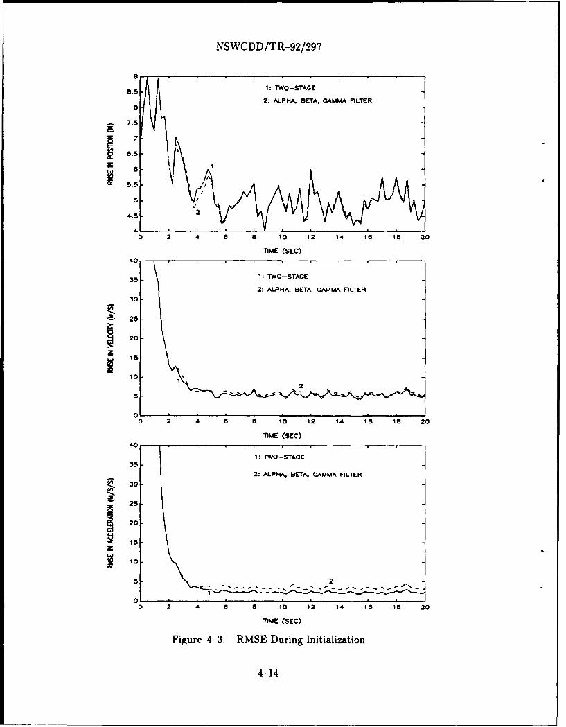
Figure 4-3 gives a comparison of the Root-Mean Square Errors (RMSE) during intial-
ization of the two-stage a, /3, I estimator with Eqs. (4.85) through (4.90), and the a, /3, -1filter with Eqs. (2.52) through (2.54). For the a,/3,8 filter, the steady-state gains were
chosen with a = 0.45. For the two-stage estimator, the steady-state gains were chosen with
a = 0.35 and ' = 0.15 to match the position variances. The errors are the average over 50
experiments. The target trajectory began at 12 km with an initial velocity of -100 m/s and
the acceleration remained constant at 10 m/s/s. The measurement period was 0.25 sec and
a,, = 8 m. The RMSE of the two filters a. losely matched in the transient region from 0
to 4 sec, while the RMSE in position are clos,_,y matched in steady-state.
When Eqs. (4.85) through (4.90) are used to initialize the two-stage estimator, the
maneuver switch can be left open until enough measurements are received so that the accel-
eration estimate is settled before it is used.
EXAMPLE
A simple tracking system is considered to illustrate the operation of the two-stage es-
timator. The tracking system measures a target's position at 4 Hz with errors that have a
standard deviation of 8 m. The target is expected to perform maneuvers with up to 2 g of
4-13
NSWCDD/TR-92/297
8.5 1: TWO-STAGE
2: ALPHA. BETA, GAMMA FILTER8
-. 7.5
7
.5-
5.5
V4..5 2
400 2 4 a a 10 12 1.4 Is 18 20
TIME (SEC)
35-\ 1: TWO-STAGE
2: ALPHA. BETA, GAMMA FILTER
30
S25-
(IQ
22
15
10 1
5-
o0 2 4 8 10 12 14 18 18 20
TIME (SEC)
40
1: TWO-STAGE
352: ALPHA. BETA, GAMMA FILTER
~30-25
15
5- 2
00 2 4 a a 10 12 14 1 18 20
TIME (SEC)
Figure 4-3. RMSE During Initialization
4-14

NSWCDD/TR-92/297
acceleration. For an a,/3, -y filter, a = 0.45, / = 0.13 and 7 = 0.02. For the two-stage esti-mator, a = 0.35,,3 = 0.075 and I = 0.15, where Eq. (4.40) was used to compute '. While
various techniques can be used for maneuver detection, a soft switch approach was chosen.
For the soft switch approach, the bias filter is duplicated in the maneuver detector with bkas the filter output. Then the gain of the maneuver switch in Eq. (4.33) is augmented by
0, IbkI < 4.0
Gss 1.0, IbkI > 6.0 (4.91)
0.5({bk - 4.0), otherwise
Also, to improve maneuver response, the magnitude of bk is restricted so that IbkI _< 6.2.
Using the soft switch approach, the correction of the output of the bias-free filter with theacceleration estimates is multiplied by Gss. Simulated tracking results from a Monte Carlosimulation with 200 experiments are given in Figure 4-4 for the two filters, where the target
moved with constant velocity except for a 2 g maneuver from 15 to 30 sec. A critically
damped, second order system with an approximate time constant of I sec was used to modelthe dynamics of the target. As indicated in Figure 4-4, the two-stage estimator providessignificantly better tracking when the target moves with constant velocity, while matching
the tracking performance of the a, fl, -y filter during the maneuver.
4-15

NSWCDD/TR-92/297
10
1 - TWO-STAGE
2: ALPHA. BETA. GAMMA FILTERa
z
S 4
3
2
1
0o 5 10 15 20 25 30 35 40 45
TIME (SEC)
20
1: TWO-STAGE182: ALPHA, BETA. GAMMA FILTER
18
~ 14--
"
. I A 2 2 A
4.
2-
00 5 10 15 20 25 30 35 40 45
TIME (SEC)
1: TWO-STAGE20- 2: ALPHA. BETA, GAMMA FILTER
15
10-
5 2
*0 , ,- I. ,
0-0 5 10 15 20 25 30 35 40 45
TIME (SEC)
Figure 4-4. RMSE in the Estimates
4-16

NSWCDD/TR-92/297
CHAPTER 5
TWO-STAGE ALPHA-BETA-GAMMA-LAMBDA ESTIMATOR
In the two-stage a, /0, 1 estimator, the position and velocity are tracked in the first stage,
which is a standard a, /P filter, and the acceleration is tracked separately in the second stage,
which is a standard single gain filter. However, when tracking two or three dimensional
target motion with two-stage a, 3, ' estimators operating separately in each coordinate,
the state estimates will be biased for targets maneuvering with constant speed because the
accelerations are time-varying. This bias in the state estimates can be reduced through the
use of the kinematic constraint for constant speed targets as in [9]. The speed of a target is
given byS = ( + + i2½(51
For a target moving at constant speed,dS-= 0 (5.2)dt
or
(i + ý + ii) = 0 (5.3)
This kinematic constraint can be incorporated in the system state of Eq. (2.1) or used as a
pseudomeasurement in conjunction with the measurement equation. While both approaches
are feasible, the second approach is more attractive because the first changes the state
equation from linear to nonlinear. In the implementation of the extended Kalman filter,
including nonlinearities in the measurement equation is computationally less expensive than
in the state equation [9]. Thus, the kinematic constraint of Eq. (5.3) is incorporated into the
filter through a pseudomeasurement as discussed in [9]. The pseudomeasurement equation
is given byVklk • Ak + P'k = 0 (5.4)Skik
where
Vk•k = [ ýI kIk 4k1k Zklk ] (5.5)
5-1
NSWCDD/TR-92/297
Skfk = ( ±lk +2k +k k) (5.6)
and Ak - N(0, R'). The Vk~k and SkIk are the filtered velocity and speed, respectively, for
time k given measurements through time k. The Yk is a white Gaussian error process that
accounts for the uncertainty in both Vklk and the constraint. Since the initial estimate of Vklk
may include a significant error, R' is initialized with a large value and allowed to decrease
as
R = ri (6)k + r0 (5.7)
where 0 < 6 < 1, r, is a constant chosen large for initialization, and ro is a constant chosen
for steady-state conditions.
The two-stage a,/3, ' estimator utilizing this constraint in the second stage will be called
the two-stage a,c/, A, A estimator. Eq. (5.4) can be written as
Wlkik + ZkIkik) = Xkl--ik + Ik (5.8)Skjk SkIk
Thus, the filtered acceleration estimates can be inserted into the left side of Eq. (5.8)to compute a measurement for updating the x-coordinate acceleration. For the two-stage
approach, the measurement equation for the z-coordinate is given by Eq. (3.6) with bk = Ak
as
[~-1kk~~ +Zk kkk) [ Xk + [C]Ak + [ VJ (5.9)
Skik (5.10)
where Yk is the x-coordinate position measurement, vk - N(0, Rk) is the measurement error,
Yk - N(0, R") is the constraint error, and Ak is the x-coordinate acceleration.
Since the bias-free state is not observed through the pseudomeasurement, its gain in the
bias-free filter can be shown to be zero. Thus, the bias-free filter can be defined as if the
kinematic constraint is not being used. Thus, as in Chapter 4, the bias-free filter of Eqs.(3.7)-(3.11) corresponds to the standard constant velocity filter when defined as in Eqs.
(4.1)-(4.5). Using Eqs. (3.17)-(3.19) in conjunction with Eq. (5.2), Uk, Vk, and the first
element of Sk can be shown to be independent of the constraint and equivalent for both thetwo-stage a, I3, estimator and the two-stage a, 3, ý, A estimator. The second element of Sk is
given by S1 = C1. Also, since the errors on the measurement and the constraint are assumed
to be independent, the measurement update and the constraint update of the bias filter will
5-2

NSWCDD/TR-92/297
be performed separately with the measurement-updated acceleration estimates being used
to compensate the velocity estimates in the pseudomeasurement. Thus, the bias filter of
Eqs. (3.12)-(3.16) corresponds to the standard constant state filter with the residuals of the
bias-free filter rk and the pseudomeasurement as the inputs. Since the bias corresponds to a
scalar acceleration, the bias filter gain includes a scalar gain for the bias-free filter residual
and a scalar gain for the constraint. Let the bias filter gain for the bias-free filter residuals
be represented byKb = 7k(Sk), k > 0 (5.11)
where ýk and S' are positive scalars obtained from Eqs. (3.15) and (3.17) with SI being the
first element of Sk. Let the gain for the constraint be represented by
h'I = AkCk, k > 0 (5.12)
where Ak is a positive scalar. Letting Ak = bk, the two-stage a, ,3, 1, A estimator is giv-n in
the following equations:
Prediction
XkIk-l = Fk-lXk-ljk-1 (5.13)
Aktk_1 = AkcIlkI (5.14)
1 k1- A3 -1 TUk = A3k-1 Uk_ + ak- (5.15)
T
Measurement Update
ExXkIk = XkIk_, + k (Yk - HkXklk_ 1 ) (5.16)
AkIk = (1 - fk)Akjk}- + !k(SkI)-'(rk) (5.17)
Constraint Update
Ackk - AkIk - Ak - 4Lk (xklkxk -+- tkj&kYIk + iklkiklk) (5.18)
Output Correction
Xkjk = Xkjk + VkAklk (5.19)
Vk -4Tk 0]Uk (5.20)
5-3

NSWCDD/TR-92/297
The velocities of Eq. (5.18) are temporarily compensated with the acceleration estimates as
in Eq. (5.11) before updating the acceleration with the kinematic constraint. The bias filter
is initialized with A01-1 = 0 and U- 1 = [0 0]T.
If the measurement rate is uniform (i.e., T is constant) and the statistics of the measure-
ment and acceleration errors are stationary (i.e., Rk =U and = t h
filter in steady-state conditions corresponds to an a, 3 filter with ak = a and 1k = 0. The
steady-sta~e values of Uk and Vk are given by Eqs. (4.18) and (4.19), respectively. Using
Eqs. (3.17) and (5.9) gives
[ C_ ]T (5.21)
where the first element of Sk reaches a steady-state value. The bias filter is a two-gain filter
with the residual of the bias-free filter multiplied by (S')- 1 and the pseudomeasurement as
inputs. Using Eq. (2.8) for the Kalman gain gives
S pb pz-2]
=k [P l: ;&W (5.22)•kC klk k 1,
where -2 is the variance of the residual errors entering into the bias filter as shown "n Eq.
(4.27), and a2 is the variance of the constraint errors. Thus, using Eq. (5.22) gives
-2Ak = 77 (5.23)
and the output variance of the second stage is given by
Pb -- 2 llk = Ika?1 = T4 (- - a) (5.24)
If the statistics of rk are stationary, the bias filter will achieve steady-state conditions when
the statistics of 1Vb are stationary (i.e., Qb = 0,) and the kinematic constraint is not
included. Thus, for simplification, the gain Yk will be assumed to reach a steady-statte value
1. Thus, the covariance matrix of the output of the two-stage a,,3,1, A estimator will the
equivalent to that of the two-stage a, 0, ' estimator given in Chapter 4.
When selecting A, the scalar relationship between A and ý of Eq. (5.23) can be adjusted
through ao,2 to tune the filter. The gain scheduling technique for initializing the two-stage
a, 13, 5 estimator given in Chapter 4 can be used for the two-stage a, 0, ),)A ectimator with
a0A v1 6 k+ II < 1 (5.25)
where ro is chosen for steady-state conditions, ri is chosen large for initialization, and b is
chosen for the desired settling time.
54

NSWCDD/TR-92/297
CHAPTER 6
SIMULATION RESULTS
As an example, a tracking system that measures a target's position at 2 Hz with errors
that have a standard deviation in range of 6 m and standard deviation in bearing and
elevation of 2 mrad. For an a, fl, -y filter, a = 0.40, / = 0.1 and y = 0.013. For the two-stage
estimator, a = 0.3, / = 0.053, and Eq. (4.41) was used to compute • = 0.19 to match the
velocity variances of the filters. For Eq. (5.25), ro = 0.75, r, = 400, and 6 = 0.75. Thus,
in steady-state conditions A = 0.14. While various teciniques can be used for maneuver
detection, a soft switch approach was chosen. For the soft switch approach, the acceleration
filter in each coordinate is duplicated in the maneuver detector with bk as the filter output.
As a result, the gain for compensating the a, / filter in each coordinate is given by
0, IbkI < 4.0
Gss= 1.0, Ibkl > 6.0 (6.1)
0.5(bkl - 4.0), otherwise
Also, to improve maneuver response, the magnitude of bk is restricted so that IbkI < 6.2.
Using the soft switch approach, the correction to the output of the bias-free filter with the
acceleration estimates is multiplied by GsS. Simulated tracking results from a Monte Carlo
simulation with 200 experiments are given in Figure 6-1 for the a, /3, 7Y filter and the two-
stage estimator with and without the kinematic constraint. For this example, the target
moved with constant velocity except for a 4 g, constant speed turn from 12 to 24 s. The
target began at a range of 17.5 km and moved at a constant speed of 300 m/s to a final range
of 9.3 km. A cr -ically damped, second order system with an approximate time constant
of 1 s was used to model the dynamics of the target. Both two-stage estimators provide
better tracking than the a, 3, - filter when the target moves with constant velocity, while
the two-stage estimator with the kinematic constraint provides the best tracking through
the maneuver.
6-1

NSWCDD/TR-92/297
55
5 0 3 • 1I \
45 -
S40 - \ I A.
S I " N\E 35- ' .'~-5 •p •• •|\ I I I
z 30\
25- 1I
20 1: TWO-STAGE2: TWO-STAGE WITH KC - - -
15- 3: ALPHA.BFTrAGAMMA FILTER
0 5 10 15 20 25 30 3.5 40
TIME (SEC)
70
60- 3'
240
40
30 5 0 1 2C 2 30 5 4:- - • 1: TWO-STAGE ' 3101 2: TWO--STAGE WITH KC
3: ALPHABETA,GAMMA FILTER
0
0 5 10 15 20 25 30 35 40
TIME (SEC)
1 : TWO-STAGE
50 2: R WO-TAfoE WITH KC
;3: ALPHABETA2GAMMA FILTER
t 20 •"
10
C\
o o 5 0 15 20• 25 30 35 40
TIME (SEGC)
Figure 6-1. RMSE for Radar Tracking Example
6-2

NSWCDD/TR-92/297
CHAPTER 7
CONCLUSIONS AND FUTURE RESEARCH
The tracking performance of the two-stage estimator can be achieved by operating ana, 0 filter in parallel with a a, P, -v filter and selecting the output of one of the filters. However,when using the soft switch approach to maneuver detection and response as presented in
Chapters 3 and 5, a second a, 0, -y filter is required so that its acceleration estimate canbe restricted during a maneuver to improve detecting the end of a maneuver. While thismultiple filter approach is feasible, it requires approximately three times the number ofcomputations for essentially the same tracking performance.
Since the two-stage a, p, ' estimator is simple, it can be implemented in current sys-tems with a modest increase in the computational burden and memory. The two-stagea, ,, 7 estimator has the potential to provide significant performance gains in the tracking of
maneuvering targets within systems that are responsible for tracking and engaging a largenumber of targets. Also, since the two-stage a, /3, ' estimator maintains an a, # filter trackat all times, the command and control decisions, as well as maneuver detection, can bemade with greater consistency with the two-stage estimator than other adaptive filteringtechniques where the gains are increased during maneuvers.
Further research is needed to develop improved maneuver response procedures for thetwo-stage estimator. Also, further research is needed to compare the tracking performances ofthe fixed-gain, two-stage estimators with other simple, adaptive tracking algorithms. Whenusing the two-stage estimator, the kinematically constrained second stage can be paralleledwith the standard second stage so that constant speed and variable speed targets can be
tracked by selecting the more accurate second stage. However, research is needed to develop
procedures for selecting the more accurate second stage.
7-1

NSWCDD/TR-92/297
REFERENCES
1. Kalata, P.R., "The Tracking Index: A Generalized Parameter for a - /3 and a -/- -yTarget Trackers," IEEE Trans. Aero. Elect. Syst., Vol. AES-20, March 1984, pp. 174-182.
2. Cantrell, B.H., Adaptive Tracking Algorithms, NRL Report, Washington, DC, April1975.
3. Blackman, S.S., Multiple-Target Tracking with Radar Applications, ARTECH House,Inc., Norwood, MA, 1986.
4. Alouani, A.T., Xia, P., Rice, T.R., and Blair, W.D., "A Two-Stage Kalman Estimatorfor State Estimation in the Presence of Random Bias and Tracking ManeuveringTargets," Proc. of 30th IEEE Conf. on Dec. and Cont., Brighton, UK, Decemeber1991, pp. 2059-2062.
5. Alouani, A.T., Xia, P., Rice, T.R., and Blair, W.D., "A Two-Stage Kalman Estimatorfor Tracking Maneuvering Targets," Proc. of IEEE 1991 Inter. Conf. on Syst., Man,Cyber., Charlottesville, VA, October 1991, pp. 761-766.
6. Bogler, P.L., "Tracking a Maneuvering Target Using Input Estimation," IEEE Trans.Aero. Elect. Syst., Vol. AES-24, May 1987, pp. 293-310.
7. Chan, Y.T., Hu, A.G.C., and Plant, J.B., "A Kalman Filter Based Tracking Schemewith Input Estimation," IEEE Trans. Aero. Elect. Syst., Vol. AES-15, March 1979, pp.237-244.
8. Bar-Shalom, Y. and Fortmann, T.E., Tracking and Data Association, Academic Press,Inc., Orlando, FL, 1988.
9. Alouani, A.T., and Blair, W.D., "Use of a Kinematic Constraint in Tracking ConstantSpeed, Maneuvering Targets," Proc. of 30th IEEE Conf. on Dec. and Cont., Brighton,UK, December 1991, pp. 2055-2058.
10. Jazwinski, A. Stochastic Processes and Filtering Theory, Academic Press, Orlando,FL, 1970.
11. Solomon, D.L., "Covariance Matrix for a - /- Filtering," IEEE Trans. Aero. Elect.Syst., Vol. AES-21, May 1988, pp. 157-159.
12. Friedland, B.,"Treatment of Bias in Recursive Filtering," IEEE Trans. Auto. Cont.,Vol. AC-14, August 1969, pp. 359-366.
13. Alouani, A.T., Rice, T.R., and Blair, W.D., "A Two-Stage Filter for State Estimationin the Presence of Dynamical Stochastic Bias," Proc. of 1992 American ControlConference, Chicago, IL, June 1992.
8-1

NSWCDD/TR-92/297
APPENDIX A
DERIVATIONS FOR ALPHA-BETA FILTER
A-i
NSWCDD/TR-92/297
A Kalman filter is often employed to filter the position measurements for estimating the
position, velocity, and/or acceleration of a target. When the target motion and measurement
models are linear and the measurement and motion modeling error processes are Gaussian,the Kalman filter provides the minimum mean-square error estimate of the target state.
When the target motion and measurement models are linear, but the noise processes are not
Gaussian, the Kalman filter is the best linear estimator of the target state in the mean-square
error sense. The dynamics model commonly assumed for a target in track is given by
Xk+1 = FkXk + Gkwk (A.1)
where wk "-, N(O, Qk) is the process noise and Fk defines a linear constraint on the dynamics.
The target state vector Xk contains the position, velocity, and acceleration of the target at
time k as well as other variables used to model the time-varying acceleration. The linear
measurement model is given by
Yk = HkXk + nk (A.2)
where Yk is usually the target position measurement and nk -, N(O, Rk). The Kalman
filtering equations associated with the state model in Eq. (A.!) and the measurement model
in Eq. (A.2) are given by the following equations.
Time Update:
XkIkI = Fk.lXk-Ilkl1 (A.3)
PkIk-I = Fk-IPk-llk-.FT 1 + Gk.lQk-IG.lGT (A.4)
Measurement Update:
gk = Pkk_.lHk [HkPklk-.HT + R•]-i (A.5)
Xkjk = XkIk_-'I + Kk[Yk - HkXklk-l (A.6)
PkIk = [I - KkHk]Pklk-l (A.7)
where Xk ": N(Xklk, Pkjk) with XkIk and Ptkk denoting the mean and error covariance of the
state estimate, respectively. The subscript notation (klj) denotes the state estimate for time
k when given measurements through time j, and Kk denotes the Kalman gain. Using the
matrix inversion lemma of [A-l1 and Eqs. (A.5) and (A.7), an alternate form of the Kalman
gain is given bykT[HT -1
Kk Pklk-k H [HkPkIk-lHk + RkPkkIHT R-1 k-1Plk T ?-1
- [I- Pk1t 1 H Rk Hk 1 Pklk luHjjRj
A-3
NSWCDD/TR-92/297
PkJk.lHT(HkPklk-lHkT + Rj 1)-kHkkPklIHTR' 1
= [I - KKHk]PklkIHTR' 1
PklkHkTRk (A.8)
The steady-state form of the Kalman filter is often used in order to reduce thecomputations required to maintain each track. In steady-state, PkIk = Pk-ljk-1, and
Pk+1jk = P•i1k-1, and Kk = Kk-1. For a Kalman filter to achieve these steady-state
conditions, the error processes, wk and nk, must have stationary statistics and the data
rate must be constant. When the noise processes are not stationary or the data rate is not
constant, a filter using the steady-state gains will provide suboptimal estimates. The a,/3
filter is the steady-state Kalman filter for tracking nearly constant velocity targets.
The a, P filter is a single coordinate filter that is based on the assumption that the
target is moving with constant velocity plus zero-mean, white Gaussian acceleration errors.
Given this assumption, the filter gains a and # are chosen as the steady-state Kalman gains
that minimize the mean-square error in the position and velocity estimates. For the a,/3
filter,
Xk=[xk k]IT (A.9)
Fk= [I T] (A.10)
G k= [T ' T (A. 11)
Hj;= [1 0) (A.12)
Rk -= 0V (A.13)
Qk = 02W (A.14)
Kk = [a A]T (A.15)
The a,/3 gains are determined as in [A-21 by solving the simultaneous equations
02r = T 4 w 2(A.16)a2 (1 -a) (.6
,3= 2(2 - a)- 4V/• - ct (A. 17)
where F is the tracking index of [A-2], and a2,,, is the variance of the acceleration modeling
error.
STEADY-STATE ERROR COVARIANCE AND GAINS
A-4

NSWCDD/TR-92/297
Let the steady-state error covariance matrix of the filtered estimates for the a, # filter
be denoted as
P1l P121
Pk+llk+l = Pkjk = P P12 P22 (A.18)
Using Eqs. (A.8), (A.12), and (A.13) gives the steady-state gain
K = pH1To' 2 = PH (A.19)LP12 i
Thus using Eq. (A.15) gives
Pll = aO2 (A.20)
P12 = (A.21)
Inserting Eq. (A.4) into Eq. (A.7) and setting Pkik = Pk-1lk-1 = P for steady-state gives[I - KHk]-'P =FkPFL T T 1.2 (A.22)[I - ~k]-I = FtIpFT_ + Gk-,Gk-1
Then1 0
-1 a (A.23)I- K~k-1- 1 ct 1
2 T
[I - K.kl-'P 'v ° ]2P2(.4T T 2 (A.24
2Tp12 + T2p22 P12 + Tp22
FkPFT = P12 + Tp22 P22 ](A.25)
T4 T3'
T 2 2 4 ] (A.26)GkG~kOaw = aw T 2(.6
Equating the (2,2) elements of Eq. (A.22) gives
j22 Tc _ (A.27)
1- a -5
A-5

NSWCDD/TR-92/297
Equating the (1,2) elements of Eq. (A.22) and using Eq. (A.27) to eliminate a,, gives
,0(2a-/3) 2 (A.28)P22- (= -_- )T2-a T2or
Equating the (1,1) elements of Eq. (A.22) and using Eqs. (A.20) through (A.21) and Eqs.
(A.27) through (A.28) gives
I3 = 2(2-c)- 4vf--a (A.29)
Eqs. (A.27) and (A.30) give the steady-state gain relationships in Eqs. (A.16) and (A.17).
The steady-state error covariance in Eq. (A.18) is given by [1,81 as
S= (2a-#) (A.30)T 2(1 - a)T 2
MEASUREMENT VARIANCE REDUCTION MATRIX
The variance reduction between position and velocity estimates and the measurements
are often considered in the design and analysis of a, / filters. The variance reduction
matrix for the a, P3 filter is derived by considering the filter as a linear system with a white
noise input. The input-output relationships between the measurements Yk and XkIk can be
expressed as a linear system that is given by
Xkjk = FXk-ilk-l + GkYk (A.31)
where
1-a (1-a)T(
T
(A.33)
Using Eq. (A.31) provides the error covariance of Xkjk that results from white noise
measurement errors. That error covariance E[XklkXlk] = Sk is given by
-- T +-0-O~a2
Sk =FSkF +G G V (A.34)
A-6

NSWCDD/TR-92/297
where ao2 is the variance of the input Yk. Since Sk = Sk-1 = S3# in steady-state conditions,
Eq. (A.34) can be used to solve for elements of S,8 in terms of the filter gains, measurement
period, and the measurement error variance. Eq. (A.34) can be rewritten as
+ +ro T (A.35)
where
F [1 - /3 (1 2- ] (A.36)
-T ~2 ~ (a - #)a (a ~ 1(.7F-1 G av 82 1T•a (A.37)
Let
So-- 11 S21 (A.38)L S21 S22 J
Then, equating the (1,1), (2,1), and (2,2) elements of Eq. (A.35) gives
1(2 - a) - /3sii - (2 - a)(1 - a)Ts•2 = (a - /3)aav (A.39)
/3s1 + a(1 - a)Ts1 2 - (1 - a)2T 22 = = aa2, (A.40)
(2 - a)sl2 + (1 - a)Ts2 2 = =- _ (A.41)T
Multiplying Eq. (A.41) by (1 - a)T and adding it to Eq. (A.40) gives
= -2(1 - T 2 (A.42)811--- -21 -a)'•s 1 2 +t O~,,
Inserting Eq. (A.42) into Eq. (A.39) givesS12 = (2a-03)03 a2 (A.43)
a[4 - 2a - #3]T (A43
Inserting Eq. (A.43) into Eq. (A.42) gives
2a 2 + /(2 - 3a) 2 (A.44)s= -2a- - a -
Inserting Eq. (A.43) into Eq. (A.41) gives
2222 2 (A.45)a[4 - 2c - O]T; •
A-7

NSWCDD/TR-92/297
Eqs. (A.43) through (A.45) with Eq. (A.38) gives
[22a2 + #3(2 - 3a) ý(2a - /)(.62/•__T 22 ] (A.46)ad,~~- ~(2a - P) 2
where dl = 4-2a-fl. The variance reduction ratios of the filter are given by Eq. (A.46) when
a2 = 1 with the (1,1) and (2,2) elements of S3, denoting the position variance reduction
ratio and velocity variance reduction ratio, respectively [A-3].
INITIALIZATION GAINS
For tracking systems with a uniform data rate and stationary measurement noise,
nonmaneu- .-ring targets can be accurately tracked with a steady-state Kalman filter.
However, between filter initialization and steady-state conditions, the Kalman gain and
state error covariances are transient. If steady-state gains are used from initialization, the
settling time of the state estimates may be extended significantly. While the initial gains can
be approximated as decaying exponentials as suggested in [A-2], identifying the constants
for the exponential can be quite cumbersome. The purpose of this section is to present a
simple gain scheduling procedure for initializing a, #3 filters.
The gain scheduling procedures are developed by using the motion and measurement
models to formulate a batch least-squares estimation problem for an arbitrary number of
measurements. An analytical form is then obtained for the resulting error covariance that is
used in conjunction with Eq. (A.8) to obtain an analytical form for the Kalman gain.
For linear least-squares estimation, an equation formulating the measurement vector
Z as a linear function of the parameter vector X to be estimated is given by
Z= WX+V (A.47)
where E[V] = 0 and E[VVT] = a 2IN for N measurements with IN denoting the N x N
identity matrix. The least-squares estimate X is given in [A-4] as
c -= (WTW)-IWTZ (A.48)
with error covariance
PN = COV[.k] = a 2(WTW)-y (A.49)
A-8

NSWCDD/TR-92/297
A current state estimate of X denoted by Xo = [x0 io] can be obtained from thecurrent measurement plus the N previous measurements as
ZN = WNXO + VN (A.50)
where
ZN = [y-N Y-N+I ... Y-1 YO (A.51)
VN = iv-N V-N+i ... V-1 vo]T (A.52)
1 1T-NT (-N+1)T ... -T 0(A.53)
with E[VN] - 0 and E[VNVk] = a2gIN. The error covariance of the least-squares estimate
Xo is given by
COV[Xo] = = a,(WNTWN) (A.54)
First,
N
N + 1 TE(-N + i)/=0(WNTWN)= Nv N
TE(-N + i) T2E(N- i)2
i=O i=o
NN + I -TEJ
j=0 (A.55)N N
-TI:j T2 Zj 12
j=0 j=0
Evaluating the finite summations of Eq. (A.55) gives
1 -N T
2
Then
COV[Xo] = PN
222N+l IaI T (A.57)(N + 1)(N + 2) 3 6
T (N- l)T 2
A-9

NSWCDD/TR-92/297
Let the Kalman gain be denoted by
Kk=[k -]T (A.58)
Letting PkIk = Pk in Eq. (A.8) provides a simple gain scheduling procedure for a and •
during initialization that is given by
2(2k + 1) (A.59)aj = max{(k +( 2)(k +A.
=k max{(k + 1)(k +2)'•} (A.60)
with X01-1 = [0 0 ]T. Note that if Yo/T can be extremely large relative to dynamic range
of the computer, the first two filter iterations should be computed analytically to use a
two-point initialization procedure.
A-10
NSWCDD/TR-92/297
REFERENCES
A-1. Jazwinski, A. Stochastic Processes and Filtering Theory, Academic Press, Orlando,FL, 1970.
A-2. Kalata, P.R., "The Tracking Index: A Generalized Parameter for a - / and a -/3 --yTarget Trackers," IEEE Trans. Aero. Elect. Syst., Vol. AES-20, March 1984, pp. 174-182.
A-3. Blackman, S.S., Multiple-Target Tracking with Radar Applications, ARTECH House,Inc., Norwood, MA, 1986.
A-4. Luenberger., D.G., Optimization By Vector Space Methods, John Wiley & Sons, Inc.,New York, NY, 1969.
A-1I
NSWCDD/TR-92/297
APPENDIX B
DERIVATIONS FOR ALPHA-BETA-GAMMA FILTER
B-1

NSWCDD/TR-92/297
A Kalman filter is often emplced to filter the position measurements for estimating the
position, velocity, and/or acceleration of a target. When the target motion and measurement
models are linear and the measurement and motion modeling error processes are Gaussian,
the Kalman filter provides the minimum mean-square error estimate of the target state.When the target motion and measurement models are linear, but the noise processes are not
Gaussian, the Kalman filter is the best linear estimator of the target state in the mean-square
error sense. The dynamics model commonly assumed for a target in track is given by
Xk+j = FkXk + Gkwk (B.1)
where wk - N(O, Qk) is the process noise and Fk defines a linear constraint on the dynamics.
The target state vector Xk contains the position, velocity, and acceleration of the target at
time k, as well as other variables used to model the time-varying acceleration. The linear
measurement model is given by
Yk = HkXk +flk (B.2)
where Yk is usually the target position measurement and nk - N(O, Rk). The Kalman
filtering equations associated with the state model in Eq. (B.1) and the measurement model
in Eq. (B.2) are given by the following equations.
Time Update:
XkIk..1 = Fk.lXk-Ilk-. (B.3)
PkIk-, = Fk-,1Pk-Ik..F Tl + Gk..Qk-.GT (B.4)
Measurement Update:
Kk = PkIk_,H T[HkPklk_,H' + Rk]' (B.5)
Xkjk = XkIk-l,+ Kk[Yk - HkXklk-,] (B.6)
PkIk = [I - KkHk]Pkk-. (B.7)
where Xk - N(Xklk, Pkjk) with Xkjk and PkIk denoting the mean and error covariance of the
state estimate, respectively. The subscript notation (klj) denotes the state estimate for time
k when given measurements through time j, and Kk denotes the Kalman gain. Using the
matrix inversion lemma of [B-1 and Eqs. (B.5) and (B.7), an alternate form of the Kalman
gain is given byT fT +R1
Kk = Pklk-IHk [HkPklkIHLk + k
= [I- P- k_,HTRk 'Hk]-'Pklk_,HT-'
B-3

NSWCDD/TR-92/297
Pklk-lHkj(HkPkIk-.lHT + R-k1)'H]PkiklHkRio
= [I - KkHk]Pkik_,HjR-j 1
= PkjkIHTR-1 (B.8)
The steady-state form of the Kalman filter is often used in order to reduce thecomputations required to maintain each track. In steady-state, PkIk = Pk-Ilk-1, and
Pk+Ilk = Ptkk-1, and Kk = Kk-I. For a Kalman filter to achieve these steady-stateconditions, the error processes, wk and nk, must have stationary statistics and the datarate must be constant. When the noise processes are not stationary or the data rate is notconstant, a filter using the steady-state gains will provide suboptimal estimates. The of, /, 7
filter is the steady-state Kalman filter for tracking nearly constant acceleration targets.
The a,/3, - filter is a single coordinate filter that is based on the assumption that thetarget is moving with constant acceleration plus zero-mean, white Gaussian accelerationerrors. Given this assumption, the a, 3,7y filter gains are chosen as the steady-state
Kalman gains that minimize the mean-square error in the position, velocity, and accelerationestimates. For the a,/3, y filter,
x=[= k Xk k ik (B.9)
[1 T 0.5T 2 1Fk= 0 1 (B.10)
0 0
Gjk= --2 T 1 (B.11)
Hk=[1 0 0] (B.12)
Rk = a.2 (B.13)
Qk = arW (B.14)
Kk=a = A ]T (B.15)
The a,/3, -y gains are determined as in [B-2] by solving the simultaneous equationsT 2 •2T, -, (1 2 •)(B.16)U2V (1a)
0 = 2(2 - a) - 4v/ -.,1 (B.17)=32 (B.18)
2a
where F Tw is the tracking index of [B-2].Ov
B-4
NSWCDD/TR-92/297
STEADY-STATE ERROR COVARIANCE AND GAINS
Let the steady-state error covariance matrix of the filtered estimates for the a,/3,3"filter be denoted as
r P11 P12 P13]
P= [P12 P22 P23 (B.19)
.P13 P23 P33.
Using Eq. (B.8), (B.12), and (B.13) gives the steady-state gain
[P11
K =PHku7 v 1 (B.20)
SP13
Thus using Eq. (B.15) gives
P11 = av (B.21)
P12 = A2 (B-.22)
P13 = 02V (B.23)
Inserting Eq. (B.4) into Eq. (B.7) and setting Pkj- P=lk-11-1 = P for steady-state
gives
[I - KHk] 1-P = Fk_iPFT_ + (B.24)
Then
1 0 0
[I-KH 1 1 - a 0 (B.25)
a TT -[I- KHk]-~1 P=1 T- 2 ' .
f. 0 1-a)aT2
[I- ~k-' ý _CL2 0- + (I -a P2 (B.26)-- -- 2 + or) f3-0,2
f_ + _' a)P23 + I a23T2 T3 0+ r2-- T4 -t ]-, 3a2
B-5

NSWCDD/TR-92/297
T4P11 + 2T9p12 + T2 (pi3 + P22) + T3p23 + --•- 33 ..
FkPF[T P12 + T (p13 + P22) + 3T2-P23 + T 3 P22 + 2Tp23 + T 2p33 ...
T2
P13 + Tp23 + -P33 P23 + Tp33 P33
(B.27)
T 4 V3 T2
4 2 2
GGkkOf,2 cr2-T T' (B.28)-TiG*Gtaw a2 T2 T (B28
2
Equating the (3,3) elements of Eq. (B.24) gives
=72 =c F2 (B.29)1- a t F2
Equating the (2,3) elements of Eq. (B.24) and using Eq. (B.29) to eliminate acw gives
733 ( -Y) o2 (B.30)(1 -c x)T 4
Equating the (2,2) elements of Eq. (B.24) and using Eq. (B.29) to eliminate a2 gives
P23 = f(0-f) O2 (B.31)
Equating the (3,1) elements of Eq. (B.24) and using Eqs. (B.20), (B.29), (B.30), and (B.31)
gives- =2 (B.32)
Equating the (2,3) elements of Eq. (B.24) and using Eqs. (B.20), (B.29), and (B.31) gives
P 4a/3 + y(/O - 2c - 4) 2 (B.33)P22 - 4(1 -- a)T 2 (B.33
Equating the (1,1) elements of Eq. (B.24) and using Eqs. (B.21) through (B.23) and Eqs.
(B.29) through (B.33) gives
2= 2(2 - or)-4 VT(B.34)
B-6

NSWCDD/TR-92/297
Eqs. (B.29), (B.32), and (B.34) give the steady-state gain relationships in Eqs. (B.16)
through (B.18). The steady-state error covariance in Eq. (B.19) is given by
j3 -
T T
P 2 1 4 a + -y(#- 2a- 4 ) 1(1-,)P T 4(1 - T2 2(1 - a)T 3 (B.35)
7 NO - -Y) ( - -y)T2 2(1 - a)T3 (I -a)T 4
INITIALIZATION GAINS
For tracking systems with a uniform data rate and stationary measurement noise,
nonmaneuvering targets can be accurately tracked with a steady-state Kalman filter.However, between filter initialization and steady-state conditions, the Kalman gain and
state error covariances are transient. If steady-state gains are used from initialization, the
settling time of the state estimates can extended significantly. While the initial gains can be
approximated as decaying exponentials as suggested in [B-2], identifying the constants for
the exponential can be quite cumbersome. The purpose of this section is to present some
simple gain scheduling procedures for initializing a, P, -t filters.
The gain scheduling procedures are developed by using the motion and measurement
models to formulate a batch least-squares estimation problem for an arbitrary number of
measurements. An analytical form is then obtained for the resulting error covariance that is
used in conjunction with Eq. (B.8) to obtain an analytical form for the Kalman gain.
For linear least-squares estimation, an equation for:nulating the measurement vector
Z as a linear function of the parameter vector X to be estimated is given by
Z = WX + V (B.36)
where E(V] = 0 and E[VVTI = a2 IN for N measurements with IN denoting the N x N
identity matrix. The least-squares estimate X is given in [B-3] as
X = (WTW)-'WrZ (B.37)
with error covariance
PN = COV[X] = a4 2(WTW)- (B.38)
B-7
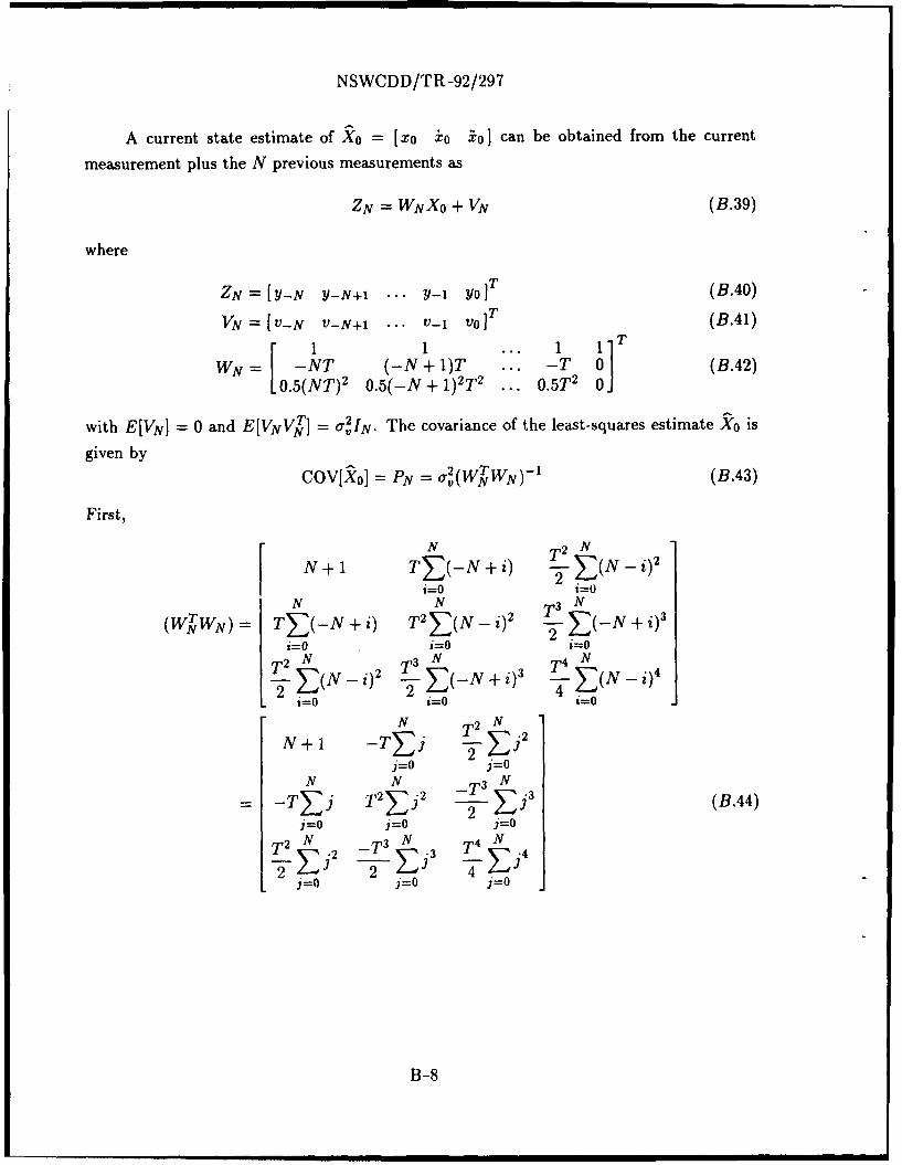
NSWCDD/TR-92/297
A current state estimate of Xo = [xo jo io] can be obtained from the current
measurement plus the N previous measurements as
ZN = WNXO + VN (B.39)
where
ZN = [Y-N Y-N+1 ... Y_1 Yo]T (B.40)VN =[v-N V-N+, ... v_, vO]T (B.41)
11 ... 1 1I]
WN = -[ T +(- 1)T ... -T 20 (B.42)[0.5(NT)2 0.5(-N + 1)2T2 ... 0.5T 0
with E[VNI - 0 and E[VNV T ] - 021N. The covariance of the least-squares estimate Xo is
given by
COV[XIo] = PN = a,(WNTWN)' (B.43)
First,
N T2 NNY+lI TE(-N +i) 2-E(N-i)
i=O i=0
TN N 2 T3 N
(WWN)= TE(-N + i) T2E(N -)2 (-N + i)3i=O i=O i=O
T2 N -2T3 N T4 N -4-2 E(N - )2 E(-N + i) 4 E(N-i)
L i=0 i=0 i=0
N 2 N
N + 1 -TEJ T EjNj=o j=o
N N _T 3 N
- TZJ T 2 ,j 2 2 E- 3 (B.44)j=O j=O j=O
T 2 N _T 3 N T4 N-j 4sE Ej4j=0 j=o i=o
B-8

NSWCDD/TR-92/297
Evaluating the finite summations of Eq. (B.44) gives
(WTWN) = (N + I).
-NT N(2N + 1)T2
2 12-N T N(2N + 1)--2 -N2(N + 1)-- (B.45)
T22 T3 224N(2N + 1)- -N 2 (N + 1)T N(2N + 1)(3N 2 + 3N- I)--j
L12 8120-
Then
(WNrWN)PN = 0'2I3 (B.46)
Let the error covariance be denoted as
[all a12 a13 1PN = a2 '22 a23 (B.47)
a13 a 2 3 a 3 3.
Equating the elements of Eq. (B.46) gives the following six equations t, solve for PN:
1 72 722 2__ (.48-all - -a12 + (2N + 1) -Ta13 = V + B1)N 2 12 N'N +11 T T2
-a 12 - -a22 + (2N + 1)--2-a23 = 0 (B.49)
1 72 722-a 1 3 - T-a23 + (2N + 1)-a 33 = 0 (B.50)N 2 12T T2 T3 a,2 (.1a2 + (2N + 1)-"a22 - N(N + 1)78-a23 =
-~~ N(N +1-2 1)
T T2 T3a3=0-ja13 + (2N + 1)- 6a 23 - N(N + 1)-a 3 3 = 0 (B.52)
72 r3 T4 a2(2N + 1)-Ta13 - N(N + 1) -a23 + (2N + 1)(3N 2 + 3N - 1)(12 -. 53)
12 8 + 1 20 N(N-+ 1)
Solving Eqs. (B.48) through (B.53) gives
COV(XOJ = PN -
3N 2 + 3N + 2 6(2N + 1) 20T T2
3a_ 6(2N + 1) 4(2N + 1)(8N- 3) 120
(N + 1)(N + 2)(N + 3) T (N - 1)NT 2 (N - 1)T (20 120 24072 (N- 1)T 3 (N- 1)NT4
B-9
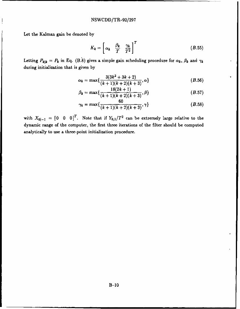
NSWCDD/TR-92/297
Let the Kalman gain be denoted by
K [ A • ]T (B.55)
Letting PkIk = Pk in Eq. (B.8) gives a simple gain scheduling procedure for ak, 13k and 7k
during initialization that is given by
3(3k 2 + 3k + 2)= max{ (k + 1)(k + 2)(k + 3)' (B.56)
flk = maxI l1(2k + 1) (.7=t max{(k + 1)(k + 2)(k + 3)'3 1 (B.57)
60k max(k + 1)(k + 2)(k+ 3)'7} (B.58)
with X0-, = 0 0 0T . Note that if Yo, 1/T 2 can be extremely large relative to the
dynamic range of the computer, the first three iterations of the filter should be computed
analytically to use a three-point initialization procedure.
B-10
NSWCDD/TR-92/297
REFERENCES
B-1. Jazwinski, A. Stochastic Processes and Filtering Theory, Academic Press, Orlando,FL, 1970.
B-2. Kalata, P.R., "The Tracking Index: A Generalized Parameter for a - /3 and a - / - yTarget Trackers," IEEE Trans. Aero. Elect. Syst., Vol. AES-20, March 1984, pp. 174-182.
B-3. Luenberger., D.G., Optimization By Vector Space Methods, John Wiley & Sons, Inc.,New York, NY, 1969.
B-11

NSWCDD/TR-92/297
DISTRIBUTION
Copies Copies
ATTN GEORGE SIOURIS 1 ATTN DR GEORGE SWISHERASC/ENSSC COLLEGE OF ENGINEERINGWRIGHT PATTERSON AFB OH 45433 TENNESSEE TECHNOLOGICAL UNIV
TTU BOX 05005ATTN DRRABINDERMADAN 1114SE 1 COOKEVILLE TN 38505CHIEF OF NAVAL RESEARCH800 N QUINCY STARLINGTON VA 22217-5000 ATTN DR PAUL KALATA
ECE DEPARTMENTATTN DR GLENN M SPARKS 1 DREXEL UNIVERSITY
ANTHONY VIDMARJR 1 PHILADELPHA PA 19104GOVERNMENT ELECTRONIC SYSTEMS
DIVISION ATTN EDWARD PRICEGENERAL ELECTRIC COMPANY SCOTT GODFREYMOORESTOWN NJ 08057 LON CARPENTER
FMC CORPORATIONATTN PROF YAAKOV BAR SALOAM 1 1 DANUBE DR
DON LERRO 1 KING GEORGE VA 22485ESE DEPARTMENT U 157260 GLENBROOK RD ATTN JOSEPH S PRIMERANOSTORRS CT 06269-3157 RAYTHEON
PO BOX 161ATTN WILLIAM STONESTREET DAHLGRENi VA 22448ALPHATECEXECUTIVE PLACE III ATTN DRRAGHAVAN50 MALL RD LNK CORPORATIONBURLINGTON MA 01803 6800 KENNELWORTH AVE
STE 306ATTN OLIVER E DRUMMOND RIVERDALE MD 20737
PH D PROFESSIONAL ENGINEER 1GENERAL DYNAMICS ATTN GLENN WOODARDAIR DEFENSE SYSTEMS DIVISION SYSCON CORPORATION10900 E 4TH ST TIDEWATER DIVISIONMZ 601 75 PO BOX 1480RANCHO CUCAMONGA CA 91730 DAHLGREN VA 22448-1480
ATTN DR J N ANDERSON 1 DEFENSE TECHNICAL INFORMATIONA T ALOUANI 1 CENTERP K RAJAN 1 CAMERON STATION
DEPARTMENT OF ELECTRICAL ALEXANDRIA VA 22304-6145 12ENGINEERING
TENNESSEE TECHNOLOGICAL UNIV ATTN GIFT AND EXCHANGE DIV 4TTU BOX 05004 LIBRARY OF CONGRESSCOOKEVILLE TN 38505 WASHINGTON DC 20540
(1)

NSWCDD/TR-92/297
DISTRIBUTION (CONTINUED)
Copies Copies
INTERNAL DISTRIBUTION: N05 1N05 (GASTON) 1
E231 3 N07 1E261 (SWANSBURG) 1 N24 1E32 (GIDEP) 1 N24 (BAILEY) 1F21 1 N24 (HANSEN) 1F21 (PARKER) 1 N24 (MILLER) 1F21 (RYAN) 1 N24 (BURROW) 1F32 (HILTON) 1 N24 (SERAKOS) 1F41 2 N32 (CURRY) 1F41 (TANNER) 1 N35 (BOYER) 1F41 (MARTIN) I N35 (HELMICK) 1F41 (KNICELEY) 1 N35 (HARTER) 1F42 2 N35 (BAILEY) 1F42 (KLOCHAK) 1 N35 (FENNEMORE) 1F44 1G 1G05 1G06 1G07 1G11 (DOSSETT) 1Gl1 (GROVES) 1Gll (LUCAS) 1G13 (BEUGLASS) 1G20 1G23 (OHLENMEYER) 1G23 (JOHN BIBEL) 1G23 (MALYEVAC) 1G43 (GRAFF) 1G70 1G702 (AUGER) 1G706 (BUSCH) 1G71 1G71 (BLAIR) 30G71 (RICE) 1G71 (GRAY) 1G71 (HART) 1G71 (LAMBERTSON) 1G71 (MCNATT) 1G71 (PALEN) 1G71 (MURRAY) 2G71 (CONTE) 1G71 (WATSON) 2G72 (GENTRY) 1G72 (BOYKIN) 1G73 (FONTANA) 1
(2)

REPORT DOCUMENTATION PAGE Form ApprovedI OMB No 0704-0188
Publi repoting burden tor this collection ot nto andtiOnl Is e~ttlidted IC aVeraqe I hour per response. inchtudmig hI 1,nwe tor t•eewinig snsirur itons. $edtidiWrieAtiijr ddla -- wt-.gathefing and maintaining the ddtd needed. and Luonip•eting and reviewing the cotlil o1 iI atiori Send coiments regarding this burdel estimate or any ot.i! aspri t Ihiscolleciun of intovmi atiton. intiudingsuggelions for reducing this burden, to Washington rtleadquarlers Services. Directorate tot ltornial ion Opetations and Reports. 1215 ,:trewlrDavis Highway. Suite 1204. Arlington. VA 22202 4302ý arid to the Olri(e of Mane•elent and Budget. Paperwork Reduction Prolet (0704 0188) W •tihingtul DC 20501
1. AGENCY USE ONLY (Leave blank) 2. REPORT DATE 3. REPORT TYPE AND DATES COVERED
July 1992 Finial
4. TITLE AND SUBTITLE 5. FUNDING NUMBERS
Fixed-Gain, Two-Stage Estimators for Tracking Maneuvering Targets
6. AUTHOR(S)
W.D. Blair
7. PERFORMING ORGANIZATION NAME(S) AND ADDRESS(ES) 8. PERFORMING ORGANIZATION
REPORT NUMBER
Naval Surface Warfare Center, Dahlgren Division (Code G71) NSWCDD/TR-92i297Dahlgren, VA 22448-5000
9. SPONSORING/MONITORING AGENCY NAME(S) AND ADDRESS(ES) 10. SPONSORING'MONITORINGAGENCY REPORT NUMBER
11. SUPPLEMENTARY NOTES
12a. DISTRIBUTIONIAVAILABIUTY 12b. DISTRIBUTION CODE
Approved for public release; distribution is unlimited.
13. ABSTRACT (Maximum 200 words)
The two-stage Alpha-Beta-Gamma estimator is proposed as an alternative to adaptive gain versions of theAlpha-Beta and Alpha-Beta-Gamma filters for tracking maneuvering targets. This report accomplishesfixed-gain, variable dimension filtering with a two-stage Alpha-Beta-Gamma estimator. The two-stageAlpha-Beta-Gamma estimator is derived from the two-stage Kalman estiniator, and the noise variance andreduction matrix and steady-state error covariance matrix are given as a function of the steady-state gains. Aprocedure for filter parameter selection is also given along with a technique for maneuver response and a gainscheduling technique for initialization. The kinematic constraint for constant speed targets is alsoincorporated into the two-stage estimator to form the two-stage Alpha-Beta-Gamma-Lambda estimator.Simulation results are given for a comparison of the performances ol estimators with that of the Alpha-Beta-Gamma filter.
14. SUBJECT TERMS 15. NUMBER OF PAGES
Kalman Estimator, Filters, Alpha-Beta-Filters, Alpha-Beta-Gamma Filters, 69Steady-State Filers, Target Tracking 16. PRICE CODE
17. SECURITY CLASSIFICATION 18. SECURITY CLASSIFICATION 19. SECURITY CLASSIFICATION 20. LIMITATION OF ABSTRACT
OF REPORT OF THIS PAGE OF ABSTRACT
UNCLASSIFIED UNCLASSIFIED UNCLASSIFIED SAR
NSN 7540-01-280-5500 Stand ,d Form 298 (Rev 2-89)PNesrrlid by ANSi Std Z19 I8298 102

GENERAL INSTRUCTIONS FOR COMPLETING SF 298
The Report Documentation Page (RDP) is used in announcing and cataloging reports. It is important thatthis information be consistent with thie rest of the report, particularly the cover and its title page.Instructions for filling in each block of the form follow. It is important to stay within the lines to meetoptical scanning requirements.
Block 1. Agency Use Only (Leave blank). Block 12a. Distribution/Availability Statement.Denotes public availability or limitations. Cite any
Block 2. Report Date. Full publication date including availability to the public. Enter additional limitationsday, month, and year, if available (e.g. 1 Jan 88). Must or special markings in all capitals (e.g. NOFORN, REL,cite at least the year. ITAR).
Block 3. Type of Report and Dates Covered. Statewhether report is interim, final, etc. If applicable, enter DOD - See DoDD 5230.24, "Distributioninclusive report dates (e.g. 10 Jun 87 - 30 Jun 88). Statements on Technical Documents."
DOE - See authorities.Block 4. Title and Subtitle. A title is taken from the NASA - See Handbook NH8 2200.2part of the report that provides the most meaningful NTIS - Leave blankand complete information. When a report is preparedin more than one volume, repeat the primary title, addvolume number, and include subtitle for the specific Block 12b. Distribution Code.volume. On classified documents enter the titleclassification in parentheses.
DOD - Leave blank.Block 5. Funding Numbers. To include contract and DOE - Enter DOE distribution categories fromgrant numbers; may include program element the Standard Distribution fornumber(s), project number(s), task number(s), and Unclassified Scientific and Technicalwork unit number(s). Use the following labels: Reports.
NASA - Leave blank.C - Contract PR - Project NTIS - Leave blank.G - Grant TA - TaskPE - Program WU - Work Unit Block 13. Abstract. Include a brief (Maximum 200
Element Accession No. words) factual summary of the most significantinformation contained in the report.
BLOCK 6. Author(s). Name(s) of person(s) responsiblefor writing the report, performing the research, or Block 14. Subiect Terms. Keywords or phrasescredited with the content of the report. If editor or identifying major subjects in the report.compiler, this should follow the name(s).
Block 15. Number of Pages Enter the total numbLrBlock 7. Performing Organization Name(s) and of pages.address(es). Self-explanatory.
Block 16. Price Code. Enter appropriate price codeBlock 8. Performing Organization Report Number. (NTIS only)Enter the unique alphanumeric report number(s)assigned by the organization performing the report. Block 17.-19. Security Classifications. Self-
explanatory. Enter U.S. Security Classification inBlock 9. Sponsoring/Monitoring Agency Name(s) and accordance with U.S. Security Regulations (i.e.,Address(es). Self-explanatory. UNCLASSIFIED). If form contains classified
information, stamp classification on the top andBlock 10. Sponsoring/Monitoring Agency Re nort bottom of this page.Number. (/f Known)
Block 20. Limitation of Abstract. This block must beBlock 11. Supplementary Notes. Enter information not completed to assign a limitation to the abstract.included elsewhere such as: Prepared in cooperation Enter either UL (unlimited or SAR (same as report).with...; Trans. of...; To be published in.... When a An entry in this block is necessary if the abstract is toreport is revised, include a statement whether the new be limited. If blark, the abstract is assumed to bereport supersedes or supplements the older report. unlimited.
Standard Form 298 Back (Rev. 2-89)


