
AFWAL-TR-8 1-3036
ADA108 61i0
CAVITY OSCILLATION INCRUISE MISSILE CARRIER AIRCRAFT
H. W. BARTEL j. LLECT5j. M . M CI AVOY DED 19 1LOCK HEED-GEORGIA COMPANYSTRUCTURES TECHNOLOGY DIVISIONMARIETTA, GEOkGIA 30063
JUNE 1981
Finol Reporto For Perl,%d August 1979 to April 1981
0 Approvod for public feleose; distribution unlimited
rLIGHT DYNWMICS LABORATORYAIR FORCE WRIGHT AERONAUTICAL. LABORATORIESMAIR FORCE SYSTEMS COMMANDWRIGHT-PATTERSON AIR FORCE BASE, OHIO 4543 2 i 8

NOTICE
When Government drawings, specifications, or other data are used for any
purpose other than in connection with a definitely related Government
procurement operation, the United States Government thereby incurs no
responsibility nor any obligation whatsoever, and the fact that the govern-
ment may have formulated, furnished, or in any way supplied the said
drawings, specifications, or other data, is not to be regarded by
implication or otherwise as in any manner licensing the holder or any otherperson or corporation, or conveying any rights or permission to uiauufac-
ture, use, or sell any patented invention that may in any way be related
thereto.
This technical report has been reviewed and is approved for publication.
LEONARD L. MAW DAVEY L[SMITH, Chief
Project Manager Structural Integrity BranchStruotures & Dynamics Division
FOR THE COMMANDER:
aALPH L. KUSTER, JR., Coloael, U0AF
Chief, Structures & Dynamios Division
If yotur address has chanSed, If you wish to be removed from our mailing
"list, or it the addressee .is no longer employed by your organization please
"nott~y ~WAL/FIBE, W-P AFB, OH 45433 to help us maintain a current mailing
list.
Copies of' this report should not be returned unless return is required by
security considerations, contractural obligations, or notice on a speci01o
document.

SECURITY CLASS*VICATION OF THIk 04,13 (Whii. fle. Fn___________
REPOT DCUMNT~rON AGEREAD INSTRUCTIONSREPOT DCUMNTATON AGEBEFORE COMPLETING FORM
I.REPORT NUM13ER 2. GOVT ACCESSION No. 3. RECIP-ENTS CATALOG NUMBER
AWL-TR--81 -3036-4. TITLE (and Subtftl*) $. TYFE O~F 5EPOFj, A PERIOD COVERED
CAVITY OSCILLATION IN CRUISE MISSILE Fna ReportAugust 1979 to April 1981
CARRIR AIRRAFT6. PERFORMING ORG. REPORT NUMBER
CARRIR AIRRAFTLG8JER01567. AUTNOPI'. 11. CONI RACT OR GRANT NUMBER0a)
H-krolu W. Bortel F3361 5-79-C-3207James M. h-'.Avoy
9- PERFORMING ORG. t,0ZATION NAME AND ADDRESS 10. 1ýPPGPAM ELEMENT. PROJECT, TASK
Lo"k ieed--Georgia Co. APEA A WORK UNIT NUMBERS
j 86 S. Cobb Dr.MWrietta, GA 30063 24010131
1.CONTMOLLINO OFFICE NAME AND ADDRESS 12. REPORT DATE
Flight Dynamics Laboratory (AFWAL/FIBE) JUNE 1981Wright-Patterson AF11, OhioQ4533 ____________
14. MONITORING AGENCY NAME 4 A00RESS(It diftt.,ut (aMo Confto*hdg0d Qtt1c.) 15. SECURITY CLASS. (at hI. ropost)
UnclassifiedIS. ECL. ASSI PtCATIONtDOWNGRAOING
SCNEDULE
We DISTRIOUTION STATEMENT (at this R~opott
Approved for public release; distribution unlimited.
15. UPPLEMENTAny NOTES
cavity noise, cavity oscillation, cavity resonance, oscillatni pressures* 50. AOSTRACY tContfleIho an f~ot s Reie DIt #91nCOi**EV jed IdGM111V 6V N&tA ..a0bw)
This report discusses cavity oscillation in general, and particularly the problem of cavityoscillation in the missile bays of cruise missile carrier aircraft during missile launch. Themissile bay configurations analyzed ranged from the complete interior volume of a largetronsp'srt aircraft, to the bomb bay of a conventional bomber. All of the carrier aircraftcases evaluated were conceptual; no specific airframe models or manufacturers areidentified. The principles and technology presented are not limited to missile bays;they ore applicable to general cavities having free-stream flow velocities above Mach0.4. It is observed that above Mach 0.4 the pressure fluctuations in an oscillatingcavity may arise from: Xo) sustaineijperlodic pressure fluctuations in the prure shearlayer that radiate noise into the cov"Ify; b) sustained periodic pressure fluctuations inthe aperture shear layer that couple with the cavity volume acoustic modes (this generallyproduces by far the most intense cavity oscillation). Theotetical/empirical techniquesare presented for predicting oscillatory frequency, pressure level, pressure spatial distri-b6jtion in the cavity, and the degree of alleviation achievable with suppressors. The in-form Ion 'is based an extensive experimentation with subscole models having aperture&of 2 to 61'~&Ok cold air wall -jet flow facil ity. A bibliography is included containing
Jim 7 k'joaflole OF I 111y Is 0811"O.rVeC
96CURI4TV CLASSIFICATIO~N OF TWI1S 044K (Ws". 0~ M*7&orA)

PREFACE
This report was prepared by the Lockheed-Georgia Company, Marietta,
Georgia, for the Flight Dynamics Laboratory, Air Force Wright Aeronautical
Laboratories, Wright-Patterson Air Force Base, Ohio, under Contract
F33615-79-C-3207. The work described herein is a continuing part of the
Air Force Systems Command's exploratory development program to establish
tolerance levels and design criteria for acoustic fatigue prevention in
flight vehicles.
The work was directed under Work Unit 24010131, "Cruise Missile/Cavity
Oscillation Environments." Mr. Leonard Shaw (AFWAL/FIBE) was the Project
Engineer. The Lockheed Program Manager was Mr. Harold Bartel. The
Principal Investigators were Mr. Harold Bartel and Mr. James M. McAvoy.
For internal control, this report is identified by Lockheed as LGB1ERO156,
and is the only publication prepared under this contract. Submittal of the
technical report by the authors in April 1981 completed the technical
effort, which was begun in August 1979.
Acoassion P?o
NTIS GRA&IDTIC TAR•. texiouuo od
/ Justif ication . -
jistributionu/ _
Availability CodesAvail and/os,
Dist Special
)M
TABLE OF CONTENTS
Section Title Page
LIST OF FIGURES Vii
SYMBOLS AND SUBSCRIPTS Xii
1.0 SUMMARY 1
2.0 INTRODUCTION 3
3.0 TECHNICAL DISCUSSION 4
3.1 Missile Bay Configurations 4
3.2 Historical Highlights 5
3.3 Approach to Methods Development 7
3.4 Testing Arrangement 7
3.4.1 Test Facility 7
3.4.2 Subscale Models
3..,3 Data Acquisition
3.5 Exploratory Tests H
3.5.1 Cavity Oscillation 11
3.5.2 Helmholtz Resonance 14
3.5.3 Cavity Acoustic Resonance I5
3.6 CNCA Missile Bay Model Tests 20
•, 3.,v . • ~ mX gN1 .j...

TABLE OF CONTENTS (Contd)
Section Title Pag
3.7 Development of Prediction Methods 233.7.1 Missile Bay Oscillation Frequency 233.7.2 Oscillation Mode Priority 283.7.3 Distortion 303.7.4 Correlation With Prior Experiments 31
3.7.5 Sound Pressure Level Prediction 323.7.6 Sound Pressure Spatial Variation 33
3.7.7 Broadband Noise 373.7.8 Clutter Effects 38
3.8 Cavity Oscillation Predictions 403.8.1 CMCA Cases 403.8.2 Sample Application of Methods 41
3.8.3 Results of Predictions 51
3.8.4 Required Alleviation 51
3.8.5 Effectiveness of Alleviation Devices 513.8.6 Revised Predictions 54
4.0 OBSERVATIONS AND CONCLUSIONS 55
5.0 RECOMMENDATIONS 57
6.0 REFERENCES 59
7.0 BIBLIOGRAPHY 61
vi
LIST OF FIGURES
Figure Title page
1 Cavity Arrangements In Cruise Missile Carrier 7AAircraft and In Conventional Bombers
2 Long CMCA Missile Bays Selected For Analyses 75
3 Short CMCA Missile Bays Selected For Analyses 76
4 Aft Launch And Conventional CMCA Missile Bays 77Selected For Analyses
5 Generic Representation Of Missile Bays 78
6 Generic Representation Of Missile Bays 79
7 Wall-Jet Flow Facility 80
8 Aperture Viewed From Back Side Of Flow Plane, 81With A Test Model In Position
9 Typical Model Construction Concepts 82
10 Category I and Category 2 Models 91
11 Category 3 Model with Two Aperture Configurations, 84and Installation In Flow Stream
12 Category 4 Model With Spacers to Vary L/D 85
13 Response Spectra Measured At Various Flow A6Velocities. Rectangular Cavity, 18" x 5.75" x5.75" With 0.5" Neck, Aperture Located At Down-stream End
14 Frequency And Mach Number Of Oscillatory R0esponsesExceeding 150 db, In Six Variationa Of RectangularMissile Bays
15 Frequency And Mach Number Of Responses In A Ree- 88tangular 18" x 5.75" x 5.75" Missile Bay With A6" Aperture
16 Helmholtz Response In A Large Missile Bay Equipped 89With A Neck
17 Cavity Depth Correction For Depthwiae Acoustic Nodes 90In Conventional Bomb Bays
18 Cavity Depth Correction For Depthwise Acoustic Modes 9)In Category 4 MLssile Bays
vii
LIST OF FIGURES (Contd)
Figure Title Page
19 Fore-Aft Acoustic Resonance Frequencies Calculated 92And Measured In A 44" Missile Bay
20 CMCA Case 1 Response Test Spectra. Cylindrical 03Missile Bay 23.2" x 5.4" D
21 CMCA Case 2 Response Test Spectra, Rectangular Q4Missile Bay 23.2" x 5.75" x 5.75"
22 CMCA Case 3 Response Test Spectra, Cylindrical 95Missile Bay 6" x 5.4" D
23 CMCA Case 4 Response Test Spectra, Rectangular 96Missile Bay 6" x 5.75" x 5.75"
24 CMCA Case 5 Response Test Spectra, Cylindrical 97Missile Bay 7" x .85" D, Aft Launch
25 CMCA Case 6 Response Test Spectra, Conventional 93Bomb Bay, 6" Aperture, 3" Depth
26 Computed Shear Layer And Acoustic Modes. Cylindrical 99Missile Bay, 21" x 5.40 D, With 6" Aperture
27 Cavity Oscillations Measured In A Cylindrical 100Missile Bay With Floor
28 CavKLy Oscillations Measured In A Cylindrical l10Missilv. Bay, No Floor
29 Mach Number (MH) At Which The Strouhal Curves 102For Acoustic Modes And Shear Layer Modes Intersect
30 Strouhal Number (Si) At Which The Strouhal Curves 102For Acoustic Modes And Shear Layer Modes Intersect
31 Examples Of Oscillatory Sound Pressure Wave 113Distortion
32 Response Spectra Measured In A Cylindrical Missile ]14Bay, 21" x 5.40 0, No Floor, 6" Aperture At Down-stream End
33 SPL Spatial Variation Fore-Aft In 21" x 5.4" D 1)5Cylindrical Missile Bay, At ,81 Mach, 320 And,%0 Hertz Modes
34 SPL Spatial Variation Fore-Aft In 21' x 5.14" DICylindrical Missile Bay, At .81 Mach, 960 And1275 Hertz Modes
viii
LIST OF FIGURES (Contd)
Figure Title Page
35 SPL Spatial Variation Fore-Aft In 21' x 5.4" D 106Cylindrical Missile Bay, At .81 Mach, 2550 And
3825 Hertz Modes
36 Rossiter's Measured Oscillatory Response (From 107Reference 2) Correlated With Predicted AcousticModes For L/D = 1 Cavity, L = 8"
37 Rossiter's Measured Oscillatory Response (From 108Reference 2) Correlated With Predicted AcousticModes For L/D = 2 Cavity, L = 8"
38 Rossiter's Measured Oscillatory Response (From 109M/Reference 2) Correlated With Predicted Acoustic
"='--Z---••ii •Modes For L/D = 8 Cavity, L = 8"
39 Development Of Sound Pressure Level Empirical 11VPrediction Curve
40 Normalized Maximum Oscillatory SPL In Cylindrical 110Missile Bays
41 Normalized Maximum Oscillatory SPL In Rectangular 111Missile Bays
42 Normalized Maximum Oscillatory SPL In Conventional 111
Womb Bays
43 Oscillatory SPL Variation With Mach Number Between 112Onset And Termination
44 Free Stream Dynamic Pressure, Standard Atmosphere 113
45 SPL Spatial Variation Fore-Aft In 21" x 5.4" D 114Cylinderical Missile Bay, At .71 Mach, 325 And
650 Hertz
46 SPL Spatial Variation Fore-Aft In 21" x 5.4" D 114Cylindrical Missile Bay. At .71 Manh, 975 And1300 Hertz
47 SPL Variation Measured Fore-Aft In 21" x 5,4" D 115Cylindrical Missile Bay. At .71 Mach, 1600 And1775 Hertz
48 SPL Variation Measured Fore-Aft In 21" x 5.4" D 115Cylindrical Missile Bay, At .71 Mach, 1950 And2250 Hertz
:; ix

LIST OF FIGURES (Contd)
Fi~u'e Title Page
49 Fore-Aft SPL Variation Given By Equation 34 Which 116Accounts For Broadband Noise Level, 21" CylindricalMissile Bay
50 Broadband SPL At Downstream Wall Near Aperture 117
51 Depthwise Variation of Broadband SPL On Downstream 117End Wall
52 Effect Of Clutter On Frequency And Level Of Maximum 118Oscillation
53 Effect Of Clutter And Partial Blockage On Frequency 119And Level Of Maximum Oscillation
a.. 54 Shear Layer Oscillation Modes 120
55 CKCA Case 2 Predicted Acoustic Modes Superimposed OnShear Layer Modes
56 Speed Ranges Of Probable Modes Of Oscillation Predicted 122For CHCA Case 2
57 CMCA Case 2.Maximum Oscillatory Frequency And Maximum 123SPL Predicted For 25.000 Feet
58 CMCA Case 3 Maximum Oscillatory Sound Presure Spectrum 123Predicted For .6M, 25,000 Feet
5HCA Case ? Predicted Variation In SPL Fore-A~t, For 124.. M At 25,000 Feet
60 Predicted CMCA Missile Bay Oscillation Within The Speed 125Range Of .4M To 1.2M, At 25,000 feet
61 Predicted CMCA Hissile fay Oscillation At .8 Mach 126Altitudes Of 25,000 Arnd 37.000 Feet
62 CMCA Case 1 Predicted Fore-Aft Variation In SPL On 12?Wall Opposite Aperture, For .8M At 25,000 Feet Altitude
63 CMCA Case 3 Predicted Fore-Aft Variation In SPL On 12AWall Opposite Aperture, For .8M At 25,000 Feet Altitude
6P CMCA Case 4 Predicted Fore-9ft Variation In SPL On 128Wall Opposite Aperture, For .8H At 25,000 Feet Altitude
LIST OF FIGURES (Contd)
Figure Title Page
65 CMCA Case 6 Predicted Fore-Aft Variation In SPL On 12•Wall Opposite Aperture, For .8H At 25,000 Feet Altitude
66 CMCA Case 6 Predicted Depthwise Variation In SPL On 3nDownstream Wall, For .8M At 25,000 Feet Altitude
67 Illustration Of Shear Layer Alteration Devices Examined 131
68 CMCA Case 1 Response Spectra With And Without Spoiler/ 132Ramp Alleviation Devices
69 Illustration Of Selected Alleviation Devices For Long 133Missile Bays
70 Effect Of Selected Alleviation Device(s) On Maximum 133Oscillatory SPL
71 Predicted Maximum Levels Of CMCA Missile Bay Oscilla-tion With And Without Alleviation; Launch At .8 Mach,25.000 And 37.000 Feet Altitude
SYMBOLS AND SUBSCRIPTS
SYMBOLS
a Missile bay normalized dimension in fore-aft or streamwise direction;
ratio of aperture length to missile bay length; a = Lx/ ex"
b Hiisile bay normalized dimension in depth direction; ratio of aperture
length to missile bay dopth; b = Lx/ IF'
C Speed of sound in missile bay (feet per second).
C®O Speed of sound in freestream (feet per second).
D Depth dimension in open bomb bays, or diameter of cylindrical missile bayI. model,
du Decibels, alway3 referenced to 2.9006 01O"9 psi (.0002 dynes per sq. cm.).
dBr Decibel spectriu level.
F Acoustic mode order term for modes in non streamwise direction. For on-
closed rectangular missile bay3. F - N. For en-oseii cylindrical and
34micylindrlcal missile bays, F t am^* For open bomb bays, F Z 1•,I2.
f Frequency in Hertz (cycles per second).
g X'ravitational acceleration constant.
G Acoustic m*de-dependent constant defined as, G (a N bF) F I2
KNach-dependent constant defined as, R c (1+, 2
K V Ratio of convection velocity to freestream velocity. Herein, K. - 0.57.
)Li

SYMBOLS AND SUBSCRIPTS (Contd)
L,LL Aperture length in fore-aft or streamwise direction (feet).x
L y Aperture width, crosswise to stream flow (feet).
L Aperture neck or throat depth (feet).
Missile bay dimension in non-streamwise direction (feet). For enclosed
rectangular bays, IF = 1z For enclosed cylindrical and semicylindrical
missile bays, F = r. For open bomb bays, AF z
ix Missild bay 'dimension in fore-aft or streamwise direction (feet).
1I Missile bay dimension in depth direction (feet).
Aze Acoustic effective depth in open bomb bays (feet).
M Mach number.
m Tangential acoustic mode integer in cylindrical and semicylindrical en-
* closures; m 0,1,2,3, etc. (all integers).
N R 'hear layer pressure oscillation mode integer in Rossiter equation;
N R 1,2,3, etc.
Ns Shear layer pressure oscillation mode integer in Spee equation;
N 1,2,3, etc.
R: .x Fo.re-aft acoustic mode integer. In all missile bays x 0,1,2,3, etc.
(a(ll integers).
N Depthwise acoustic mode integer. In enclosed rectangular missile bays,zN = 0,1,2,3, etc. (all integer*). in open bomb bays, N 0,1,3,5 etc.z z
(odd in'egers only).
xiii

SYMBOLS AND SUBSCRIPTS (Contd)
n Radial acoustic mode integer in cylinurical and semicylindrical en-
closures; n = 0,1,2,3 etc. (ali int.6ers).
P Pressure in pounds per square inch.
q Dynamic pressure in pounds per square inch.
R Universal kas constant; 53.3, fcr air.
r Radius of cylinderical or zerx:icylino.;rical niossile bay (feet).
S Strouhal number; defined as S = fL/b.
SPL Sound pressure lev:. , . cibels.
T Temperature, degrees hankine.
U Free-stream velocity (feet per second).
U C Gonvectlon velocity (feet per seconu). hereiin U0 .57 U.
x Station or position fore-aft in w•s•ile bay, with x 0 a•t ownstrewtn
wall, in units consistent with
Station or position depthw•st in missile bay, with z -- 0 ,it aperature, inr
units eonsistant wlthl Z"
a L/D - dependent constant in hossiter equation. Herein, a .25.
amn Acoustie mode conistant for cylindrical and semicylinorical enclosures.
Quantified ilt Section 3.5.3.
Y Ratio of speclfic heats; for air, Y 1.395.
iiV

SYM4BOLS AND SUBSCRIPTS (Contd)
TIX oreaftlocation in misl bay, defined as / x
YZ Depthwise location in misile bay, defined as z
Empirical expo~nen-v, defined az 22/ (SPL -SPL)
mnax B
p Density of gas.
Xv

SYMBOLS AND SUBSCRIPTS (Contd)
SUBSCRIPTS
b Denotes broadband or random noise.
F Denotes the dimension direction that is consistant with the acoustic mode
order term F.
i Denotes the intersection of Strouhal curves for shear layer and acoustic
modes.
II Denotes tangential acoustic modes.
max Denotes the spatial maximum sound pressure level during cavity
oscillation.
n Denotes radial :acouti, modes.
0 Denotes onset of an oscillation
Denotes shear layer oscillation, ;is described by Rossiter.
Denotes shear layer osvilltion, as described by Spec.
r DLnotex random spectrum level.
t2. Denotes temtninatiot of an oscillatory condition. Also denotes total Wirn
related to temperature.
St, Denotes static.
x Denotes fore-aft or streamwise direction.
y De,,oes directio. crosswise to stream flow.
S• xvi

SYMBOLS AND SUBSCRIPTS (Contd)
z Denotes depthwise direction.
ze Denotes "effective" dimension.
Denotes free-stream properties.
11 Denotes a fore-aft or depth position in missile bay.
& :!
I,.,
I!!i: .t

1.0 SUMMARY
Approximately 30 combinations of missile bay configurations and candidate
Cruise Missile Carrier Aircraft (CMCA) were identified and studied. The
missile bay configurations were grouped into four categories related to
missile bay shapes and launch techniques. All but one (the conventional
bomb bay) represented new cavity configurations and flow conditions not
addressed by the available literature. It became necessary to evaluate the
oscillatory behavior of the "unconventional" missile bays, using
inexpensive subscale models, to determine the applicability or degree of
inadequacy of existing cavity analysis methods.
Experiments were conducted using a wall-jet flow facility with a variety
of cylindrical and rectangular models of approximately 1/40 scale. These
experiments provided evidence that two different phenomena -- shear layer
oscillation and acoustic resonance within the cavity enclosure -- combine
to cause cavity oscillation. Prior research has shown that vortices are
shed from the aperture upstream lip and propagate past the aperture, pro-
ducing travelling oscillatory pressure waves whose frequency increases with
flow Mach number. Acoustic resonance frequency within the cavity enclosure
is almost constant - it changes only as total temperature changes with
Mach number - a small change at subsonic speeds. Sustained cavity
oscillation occurs when the shear layer oscillation frequency coincides
with a cavity acoustic resonance frequency. Then the two reinforce each
other to cause oscillatory pressures that can easily exceed 170 dB (an rms
pressure of 132 pounds per square foot).
Methods for estimating the shear layer oscillation frequency and the
acoustic resonance frequency were assembled and combined into analyti-
cal/graphical procedures for determining the Mach numbers where the two
coincide. This approach resulted in a method for predicting both cavity
oscillation frequency and critical Mach number. Graphical descriptions of
sound pressure level as a function of dynamic pressure and Mach number were
obtained from model tests representing various types of missile bays.
Means for rapidly predicting the oscillatory pressure levels in missile
bays were determined from the tests. Analytical expressions for the varia-
m1

tion in sound pressure level over the length and/or depth of missile bays
were developed and verified in model tests.
From Lhe large number of CMCA candidates identified, six significantly
different cases were analyzed. The cavity oscillation environment in each
of these six cases was predicted using the analysis methodology developed.
It was found that five of the cases would encounter discrete fluctuating
pressures at frequencies ranging from 5 to 50 Hertz, and at levels on the
order of 150 to 170 dB - intense enough to cause structural damage.
Devices for modifying the shear layer over the aperture were identified for
these five cases and tested on subscale models. Cavity oscillatory
pressure levels were reduced 10 to 30 dB with the devices selected, and
based on these results the cavity oscillation environments estimated for
the five "problem" CMCA cases were revised.
The quality and accuracy of cavity oscillation prediction analyses were en-
hanced as a result of this program. Further improvement is still needed.
Recommended subjects of future development work include: detailed experi-
mental investigation of the oscillating shear layer and interaction with
acoustic resonance pressure oscillations; refinement and implementation of
an acoustic finite element analysis method for quantifying acoustio
resonance frequency and mode shape in irregularly shaped enclosures;
optimizing suppression by locating spoilers so as to modify effective
aperture lengths to mismatch frequencies of shear layer oscillation and
acoustic resonance.
2

2.0 INTRODUCTION
In studies of Cruise Missile deployment, one of the options under consid-
eration is to transport and launch the missiles using existing transport
aircraft that have been modified to provide this capability. While thisoption has obvious advantages, the transport aircraft modified to the
Cruise Missile Carrier Aircraft (CMCA) configuration will be exposed to
harsh acoustical environments that have not been considered previously. In
this study the environment of concern is cavity oscillation during missile
launch. The entire fuselage interior (or a fraction thereof) will be sub-
jected to the effects of high velocity flow past the launch aperture andcan experience intense fluctuating pressures at frequencies in the range of
5 to 50 Hertz. The cavity resonance problem has been investigated in depth
for the conventional bomb bay (the special case of a rectangular enclosure
having one entire wall open to stream flow and a length-to-depth ratiousually greater than three). In the CMCA missile bays however, wide
variations in size and shape are likely, i.e., the missile bay may be muchlonger than the aperture; the aperture may be located anywhere along the
bay length; the length to depth ratio may be less than three; the missilebay may open to the aperture via a "neck"; the missile bay cross section
may be cylindrical, semicylindrical, rectangular, or even irregular.
Two arbitrary CMCA concepts are exemplified in Figure I to illustrate their
degree of departure from a conventional bomb bay (also shown). Very little
prior development work has been done on cavities representing the CMCA
variations, so the character of cavity resonance in CMCAs was unknown and
not predictable. Nevertheless, the potential for severe resonance and re-
sultant damage was clear. Thus, a need existed for analysis methods that
would afford preliminary estimates of the frequency, amplitude, and spati ii
variation of the cavity oscillatory pressures. The effort described hereinwas undertaken to develop those aalysis methods.
Sdeveop aniys3

3.0 TECHNICAL DISCUSSION
3.1 MISSILE BAY CONFIGURATIONS
For cruise missile carriers derived from aircraft already developed and in
service, the missile bay configurations are governed by two considerations:
the type of airframe; and the missile launch system.
Airframes can be classified as:
o Cargo aircraft adaptations characterized by a low continuous floor,
high wing, and large internal volume.
o Passenger aircraft adaptations characterized by a high continuous
floor, low wing, and large internal volume.
o Bomber aircraft adaptations characterized by an integral bomb bay
of limited volume.
Missile launch systems can be classified as:
o Carriage launchers fixed in position, translating missiles for
axial ejection through aft doors or tubes.
o Linear launchers fixed in position, translating missiles for ejec-
tion through bottom.
o Rotary launchers fixed or moved into position, rotating to eject
missiles through bottom or side,
A wide variety of candidate CHCA systems can be configured .from combina-
tions of these various airframe and missile launch systems. More than 30
were identified during the course cf this effort. From this collection,
six representative configurations were selected for analysis. The six
analysis cases are shown in Figures Z, 3, and 4. along with pertinent
descriptive data. In Section 3.8 the cavity oscillation prediction methods
developed herein are applied to these six cases.

For the development of prediction methods, it was concluded that all likely
missile bay configurations could be grouped into the four simplified cavity
arrangements illustrated in Figures 5 and 6. The bulk of the initial
experimental work therefore utilized models representing these four cavity
categories.
3.2 HISTORICAL HIGHLIGHTS
Some of the earliest investigations of cavity resonance were directed
toward quantifying the noise radiated away from cavities, with analytical
prediction techniques becoming available in the early 1960's. Investiga-
tions of aircraft cavity oscillation frequency and level were intensified
in the early 1950's for the B-47 and Canberra bombers and have continued at
a moderate pace to the present time.
In 1962, Plumblee, Gibson, and Lassiter (Reference 1) developed a method to
predict cavity response based on a strong mathematical treatment, with re-
sults supported by model tests. They hypothesized that acoustic modes
within the cavity were driven by boundary-layer turbulence resulting in in-
tense pressure fluctuations. Subsequent efforts to apply the method of
Plumblee, et al. proved their method to be more applicable to what laterbecame defined as "deep" cavities. Notably, though, the method provides a
way to calculate depthwise as well as lengthwise acoustic modes in a* rectangular enclosure having one entire wall open to high-speed flow.
In 1964, J. E. Rossiter (Reference 2) conducted experiments that identifiedthe source of excitation as vortices shedding from the upstream edge of the
aperture. lie formulated an analytical expression for the cavity oscilla-tion frequency that has been widely used for *shallow' cavities.
In 1970, Heller. Holmes, and Covert (Reference 3) modified and improvedRossiter's formula to correct for the speed of sound in the cavities. In1975, Smith and Shaw (Reference 4) formulated an empirical sound pressurelevel prediction 3cheme.
m.S

Since tweie, cavity oscillation problems in the bow.b bays of aircraft such
as the F-1I1A and b-1 bombers and in miscellaneous weapons pods nave led to
the undertaking of several related cavity noise investigations (Reeferences
5, 6, 7, and 8). By and large, those investigations were directed towaro
problems associated with rectangular, shallow cavity configurations. The
results of those investigations have been used extensively to define and
refine empirical methods for the prediction of sound pressure level and
frequency. One shortcoming of these methods was the inability to predict
tne onset of cavity oscillation. Investigators using these predictions
usually qualified their results with the words, "If an oscillation occurs,
it will be at the predicted frequency."
NASA-sponsored work has been done by block, Heller, and Tan concerning,
among other things, tne extention of Hossiter's work to predict cavity
oscillations below Mach 0.4 for cavities such as open lanuing gear wheel
wells. Considerable work oti cavity oscillations has also been contributed
by the academic commutlty, dealing with cavity oscillations in deroaspace
"vehicles, wind tunnel walls, and ships. Professor S. R. Elder (tReferunces
9 and 10) is currently conducting Navy-sponsored work at the U.., Naval
Academy.
in 1978, Rockwoil and Naudascher (lHeaerence !M) correlated the taodes ob-
tained by RosiLter in his original work (for LIDt 2) wit h the longitudinal
acoustic resonance in Hossiter's cavity. They assumed that ,All six walls
wore hard and neglected depth mode response. improved correlation is ob-
tilinod (,and shown herein) when the modifiod Iossiter formula is use, inconjunction with a more precise accounititg of the acoustic resonances.
U6

3.3 APPROACH TO METHODS DEVELOPMENT
The literature applicehie to cavity oscillation was reviewed for data and
methodology useful in analyses and in alleviating or suppressing oscilla-
tion. A listing of the more noteworthy publications is in the Bibliog-
raphy. The subject matter of the literature reviewed encompassed full-
scale aircraft bomb bays, wing-mounted pod cavities, optical instrument
recesses in the surfaces of aircraft and missiles, scaled models, rec-
tangular cutouts in wind tunnels and water tables, slots and irregular
cutouts in wind tunnel walls, architectural acoustics, and musical in-
struments. The literature on cavity oscillation generally fell into either
of two groups: one dealing specifically with aircraft bomb bays; the other
dealing with more general cavities but exposed to low-velocity flow. Thus,
despite the range of subject matter evaluated, very little information was
found to be directly applicable to CMCA cavity oscillation analysis. Be-
cause of this disparity, the formulation of the CMCA cavity oscillation
prediction methodology relied heavily on subscale model tests.
3.4 TEST ARRANGEMENT
Primary considerations in the subscale model tests were low overall cost,
ease of configuration change, real-time processing )f data on-line, and
direct observation of the cavity behavior.
S3.4.1 Test Facility
The principal feature of the test facility was a semi-free cold air
rectangular jet nozzle with an integral flow plane, capable of continuous
operation at velocities exceeding Mach 1.2. The overall arrangement is
shown in Figures 7 and 8.
A cylindrical plenum chamber was positioned upstream of the nozzle, with an
internal contraction cone to transition from a cylindrical to a rectangular
cross-section. A honeycomb section was positioned at the upstreav end of
the contractiOn cone to straighten the flow er ering the noz Xe. The
supply line was brought into the plenum chamber through the side with a 90°
7

turn directing the flow back against the domed end, thus dispersing the
flow throughout the plenum before entry into the honeycomb. The nozzle
flow rate was governed by a manually controlled pneumatic regulator valve
in the supply line.
A flow-plane which contained the aperture was contiguous to one wall of the
nozzle and was mounted in a vertical plane. A flow fence made of heavy
aluminum tooling plate was positioned on each side of the aperture to form,
in conjunction with the flow-plane, a deep channel projecting downstreamfrom the nozzle exit. This channel arrangement constrained the flow on
three sides while allowing expansion and secondary air entrainment oppositethe aperture. It produced the effect of a divergent nozzle at the aperture
without having a wall opposite the aperture to reflect pressure fluctua-
tions or cause acoustic resonance effects. The aperture (or opening) in
the flow p'ane was located slightly downstream of the nozzle exit (see
Figure 7). The models were attached to the back side of the flow plane,
with their opening positioned over the flow-plane aperture (see Figure 8).
Thus, the models were outside the flow to avoid physical interference with
the airstream. The velocity distribution across the aperture was con-siderably improved over that available from a free-jet nozzle, as speed
over the aperture deviated less than one percent from the velocity at thecenter of the aperture for all speeds below Each 1.0. This is illustrated
in Figure 9 for a nominal flow velocity of Mach 0.87. The boundary layer
waa examined at various speeds and locations to verify that the flow was
uniform. A velocity profile obtained at the upstream lip of the aperture
is also shown in Figure 9. The width of the flow field over the aperture
was three times the aperture width. The depth of the flow field over the
aperture was 1.3 times the aperture length. The flow-plane thickness at
the aperture was 0.080 inch.
3,A,,?.2 Smbscale Wodels
In the preliminary experiments the sealed models were configured to repre-
sent the variations In the four categories of missile bays discussed in
paragraph 3.1,. This was achieved with four basic model geometries: (1) Acylindrical crow section model (representing Oategories 1 and 2) witt, re-
8

locatable end plugs and removable floors which provided variation in cavity
length, neck length, and aperture location upstream/downstream (see Figure
10); (2) a rectangular cross section model (representing categories I and
2) with relocatable end plugs, removable "ceiling" plugs and removable
spacers to vary cavity length, cavity depth, neck length, and aperture
location upstream/downstream (see Figure 10); (3) a cylindrical (tubular)
fuselage model mounted completely immersed in the nozzle flow (representing
Category 3) with removable end fittings employing different aperture shapes
and locations to vary cavity length and flow direction relative to the
aperture (see Figure 11); and (4) a narrow rectangular cross-section model
(representing Category 4) with cavity width equal to aperture width and
with removable spacers available to vary cavity depth (see Figure 12). The
models were constructed either from 3/4 inch plywood, 1/2 inch plexiglass,
or rolled aluminum sheet. In every case checks were made to verify that
structural vibrations did not contribute to the oscillatory pressure
response of the models.
3.4.3 Data Aequtsition
The instrumentation and the test procedures were tailored to define sound
*:• pressure spectra inside the missile bays over a Mach range of 0.4 to 1.2
and a dynamic Pressure range of 200 to 2000 psf.
Microphones (1/4 inch) were located inside the models to sense pressure
fluctations. In aome instances, the microphones were permanently fixed in
thf models, For spatial surveys, the microphones were mounted In tubular
probes that were repositioned in discrete increments. The microphone
signals were amplified or attenuated t,3 necessary for maximum signal-to-
* noise ratio, using B&K Model M603 microphorc amplifiers. The microphone
data analyses were obtained ot-line with Nicolet Scientific Corpo7eation
Model 446A Foit Fourier Transform computing analyzers and companion digital
plotters.
The cavity response and the properties of the flow were recorded at
stabilized flow conditions. The frequency response spectra ware 0ob-
,. tinuously monitored on a scope display for on-line identitfication of
9
critical velocities where response changes and ipons: rrina:ima occurred.
Total head and static pressure sen_ ors .,-re mounted in the flowstream in
the vicinity of the aperture. A pitot-static survey over the aperture was
used to calibrate the fixed pressure probes to accurately indicate velocity
at the aperture. Flowstream temperature was measured in the plenum up-
stream of the contraction nozzle, where the velocity was approximately 5%
of' the velocity at the aperture and was never in excess of Mach 0.065. An
alternate temperature measurement was made slightly downstream of the
aperture.
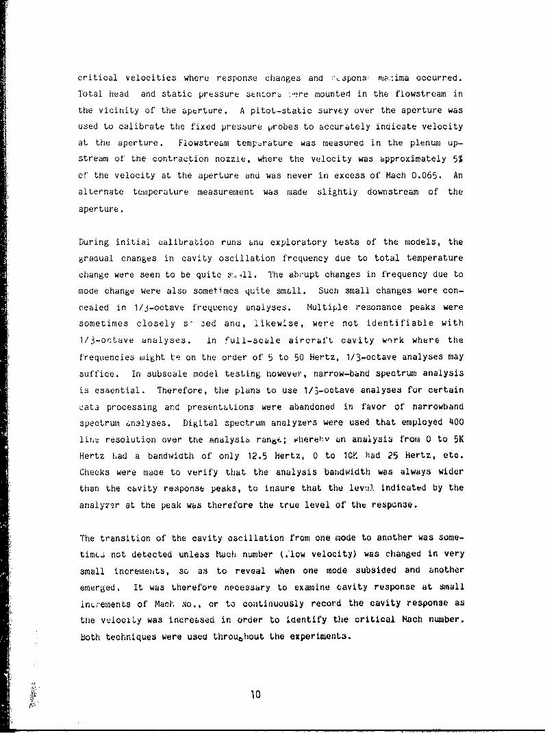
During initial calibration runs anu exploratory tests of the models, the
gradual cnanges in cavity oscillation frequency due to total temperature
change were seen to be quite sil. The abrupt changes in frequency due to
mode chan6e were also sometimes quite small. Such small changes were con-
cealed in 1/5-octave frequency analyses. Multiple resonance peaks were
sometimes closely s 2ed ano, likewise, were not identifiable with
1/3-ortave analyses. In full-scale aircraft cavity work where the
frequencies wight te on the order of 5 to 50 Hertz, 1/3-octave analyses may
suffice. In subscale model testing however, narrow-band spectrum analysis
is essential. Therefore, the plans to use 1/3-octave analyses for certain
,ata processing and presentations were abandoned in favor of narrowband
spectrum 4nslyses. Digital spectrum analyzers were used that employed 400
liriý resolution over the analysi6 range; wherehv an analysis from 0 to 5K
Hertz had a bandwidth of only 12.5 hertz, 0 to 10K had 25 hertz, etc.
Checks were maae to verify that the analysis baridwidth was always wider
than the cavity response peaks, to insure that the levt., indicated by the
analyzer at the peak was therefore the Lrue level of the respon3e.
The transition of the cavity oscillation from one miode to another was some-
tim•i not detected unless hach number (,low velocity) was changed in very
small increments, so as to reveal when one mode subsided and another
emerged. It was therefore necessary to examine cavity response at small
iný_'emens of Mach No., or to conftinuously record the cavity response as
the vwIociAy was increased in order to identify the critical Mach number.
both techniques were used throubhout the experiment3.
10

3.5 EXPLORATORY TESTS
The it:itial experiments were structured to determine that the test setup
and the subscale models provided satisfactory data and agreement with
pubiiahed results. Six variations of rectangular cross-section missile
bays were tested. These models had aperture lengths of 1/2 foot. A
typical s•:t of sound pressure level response spectra for a range of Mach
numb"rs is ;hown in Figure 13. The freqv.ptncies of the response "peaks" for
six variauions are plottea in Figure 14. The general clustering of the
data in certain frequency ranges is similar to that reported by other
investigators.
3.5.1 Cavity Oscillatiou
The solid lines in Figure 14 show the cavity oscillation frequency versus
Mach numbiier obtained with the modified hossiter equation (heference 3), for
the first 3 modal orders (N, = , 2. and 3). The mooilied Lasiter
equaotl )isU N
Lj M(]+.2M )I2 4
I-or moderate cavity length-to-depth ratio3 anu flow velocities above about
iach 0.5. the appropriate valu,,s for the constants a H and K are 0.25 and
0.57 respectively. UL is free-streami velocity; L is aperture letgth; NI,
is modal inteber (1, 2, 3 etc.); and N is freestream tiach number. The sub-'
script R denoting hossiter has been added to avoid confusion since these
symbols are also used in other equations herein. The cavity oscillation
frequency given oy the Spee equation (fieferencts 12 ana 1j) is also Shown
in Iiiure 14 for the first 3 modal orders. The Spee equation is
2T Fr~N L 2vfN Lton (2)
whfere Uc is shear loyer mean part.iele velocity, in this case taken to be
convection velocit y whichl Rossiter suggested to be 51 percent of free-

stteam velocity. While the Spee relation gave fair agreement with the data
in this comparison, it generally did not fit the data as well as the
Rossiter equation. The modified Rossiter equation was, therefore, pre-
ferred in subsequent data correlations. Figure 14 also shows that the
cavity oscillation frequency may coincide roughly with any of the first
three modal orders given by the Rossiter equation. However, there is no
indication of the mode most likely to respond for a given cavity and flow
condition. There is also considerable scatter in the data. Thus, the
frequency of oscillation is not predicted accurately with the modified
Rossiter equation clone.
A detailed study of the data revealed that over the velocity range where a
mode of cavity oscillation occurred, the frequency of oscillation often re-
mained nearly constant rather than increasing in accord with the Rossiter
equation, and generally coincided with one of the cavity acoustic
resonances through a broad speed range.
An illustration of this behavior is shown in Figure 15 for a rectangular
18" x 5.75" x 5.75" missile bay model, having a 1/2 inch neck with a one-
by-six inch aperture located at the downstream end of the cavity. The
shear layer oscillation frequency given by the Rossiter equation is shown
by the lines for NR 1, 2, and 3. The fore/aft acoustic resonance
frequencies are shown by the lines for Nx = 1, 2, 3, 4, and 5. Complex
xxacoustic modes are shown for Nx = I through 6, and Nz = 1. The frequencies
at which strong cavity oscillation occurred were obtained from the spectra
of' Figure 13 and are indicated by the solid symbols. Frequencies at which
weaker oscillation occurred (weaker but still clearly an oscillatory condi-
tion) are indicated by the open symbols. From several such experiments, it
was concluded that the shear layer instability or oscillation frequency in-
creases with Mach number approximately in accord with the modified Rossiter
equation. However, in the absence of any reinforcement from acoustic
* resonance, the shear layer oscillation is comparatively weak. At certain
velocities wh-,n the shear layer oscillation frequency approaches a cavity
acoustic resoi.w. - frequency, the shear layer oscillatiotn sometimes "looks
on" that acoustic resonance. Throughout a definite velocity range, the
* coupled shear layer/cavity oscillation occurs at the acoustic resonance
12

frequency. During this "lock on" condition, the shear layer oscillation is
reinforced and fluctuating pressures in the cavity become very intense.
Prior investigators have offered different descriptions of the mechanism
involved during this oscillatory condition. Some descriptions have dealt
with Jlow turbulence, some with captive vortices in the cavity, some with
pure vortex shedding, some with fluid inflow/outflow, and some with re-
versed flow and forward propagating pressure disturbances within the
cavity. From the current tests, it is believed that any of the previously
described mechanisms can occur under the right circumstances. It is also
believed that in some cases more complex mechanisms are involved. It was
observed that strong oscillation occurred in cavity configurations where
none of the aforementioned mechanisms seem plausible.
Neither an experimental nor thmoretical study of the aperture hydrokinetics
was within the scope of this effort. The following rationalization is thus
based on the current experiments and observations of the behavior of a
variety of widely differing cavity configurations responding in many dif-
ferent resonant modes.
The vortices that are shed from the upstream edge of the aperture give rise
to comparatively weak oscillatory pressure waves that convect downstream
over the aperture. The vortex convection velocity, hence wavelength, in-
creases with convected distance. As a result of the changing wavelength
over the aperture, a range of frequencies is available to "lock-onto"
cavity acoustic modes.
As the frequency of the convecting shear layer pressure wave nears the
frequency of an acoustic resonance in the cavity, the intensity of the
acoustic resonance standing pressure wave increases. At some frequency,
the standing wave reaches a level sufficient to "regulate" (in an unknown
manner) the shedding of the vortices, thus causing the shear layer pressure
oscillation frequency to coincide with the acoustic resonance frequency.
At this time, the acoustic pressure increases the shear layer oscillatory
pressure, which in turn increases the acoustic pressure liptil the cavity
response quickly reaches a stable but very intense level. As long as flow
13

conditions are such that the acoustic resonance pressure wave can regulate
the shear layer oscillation, the process will be sustained.
During this condition where the shear layer pressure wave is reinforced to
very intense levels, the pressures impressed on the cavity volume can be-
come severely distorted. Such a distorted wave contains higher harmonics
of the wave frequency, and readily excites higher multiples of the cavity
resonance involved.
As Mach number increases, the vortex shedding rate and hence the frequency
of shear layer oscillation is maintained until a velocity is reached where
the acoustic resonance pressure waves can no longer regulate or control the
shear layer oscillation. At this velocity, the "locked-on" condition
breaks down and the shear layer oscillation frequency reverts to the now
higher frequency as identified from the modified Rossiter equation. The
oscillatory pressure then immediately subsides to a relatively weak level.
Often however, a higher-order acoustic resonance within the cavity is
available that coincides with the ncw higher shear layer oscillation
frequency, wherein the shear layer oscillation simply "locks onto" another
acoustic resonance. Intense levels are then sustained at another
frequency. In large missile bays with many acoustic resonances available,
the cavity oscillatory condition can exist at almost all speeds above about
Mach 0.4 by simply transitioning from one mode to another as flow condi-
tions change.
As a result of many experiments, it was concluded that the formulation of
missile bay analysis methods would first require a satisfactory means fOr
quantifying the cavity acoustic resonance frequencies. In addition to the
cavity acoustic modes, the Helmholtz mode is possible in certain classes of
cavities. Both are considered in the following sections.
3.5.2 Helmholtz Resonance
The Helmholtz mode of an enclosure with an aperture may be characterized as
a single degrec-of-freedom vibration system consisting of a spring and
mass. The spring rate is determined by the elastic fluid in the enclosure
14

volume, and the mass is determined by the portion of Lair defined by the
aperture/neck geometry. Part of the fluid at the entry and exit to the
neck moves in unison with the fluid within the neck to make up this mass.
An end correction to account for the extra mass has been investigated by
Alster (Reference 14) for the case of zero flow. However, the literature
offers very little for the case of parallel subsonic flow past the aper-
ture. Since some of the CMCA missile bays involve volumes with a well-
defined neck, the behavior of the Helmholtz mode was examined in experi-
ments. The test data contained clear evidence of the Helmholtz mode at
very low speeds. The frequency of the Helmholtz mode was found to be
lowest at zero velocity and increased as speed was increased. The response
level of the Helmholtz mode was observed to always decrease above a certain
flow velocity. Any evidence of the Helmholtz mode was gone at speeds well
below the lowest launch speed. A typical Helmholtz response behavior is
exemplified in Figure 16 for a missile-bay model containing a long neck
(representative of a through-the-floor launch configuration). The response
is very sharp at M = 0.09 through M = 0.12, but is harder to identify at
M = 0.24 and completely missing at M = 0.38. This type of behavior at low
Mach number was observed on most of the missile-bay models containing well-
defined necks, but it was increasingly more difficult to identify as neck
lengths decreased to zero. As a result of these tests and observations, it
is concluded that the Helmholtz resonance can be neglected in the speed
range of interest to CHCA analysts.
3,5.3 Cavity Acoustic Resonance
Acoustic resonances in a cavity are normal modes of vibration of the air
occupying the cavity volume, and hereinafter are sometimes called acoustic
modes, or simply "modes". In a normal-mode vibration system, an infinite
number of resonant modes are possible. Any particular mode characterizes a
distinct spatial variation of the pressure in the air; likewiRe, a standing
wave characterizes an acoustic resonance.
To examine the connection between cavity oscillation frequency and cavity
acoustic resonance frequencies available, it was first necessary to
Sestablish a means for determining the acoustic resonances. Two approaches
15** " 'i

are available: (1) the use of acoustic finite element methods and (2) the
use of the classical equations for standard shapes. The works of Craggs
(Reference 15), Wolf (Reference 16), and Petyt (Reference 17) have demon-
strated the feasibility of using acoustic finite element theory to "al-
culate resonance frequency and mode shape. While tho finite element method
is capable of handling any shape, its use requires a medium-capacity
high-speed computer and a large amount of input is needed to thoroughly
define the geometry of the missile bay. The classical approach is fast and
convenient when the missile bay is idealized with an equivalent rectangular
or cylindrical cross section. The frequencies and mode shapes are then
calculated for the idealized geometry using the classical equations avail-
able from any good text on acoustics (see, for example, P. M. Morse,
Reference 18). This idealization affords considerable saving in time. The
limited number of calculations required can be made quickly on a desk
calculator. Since virtually no lateral acoustic resonance participation
occurs, the lateral degrees of freedom may be neglected. The lengthwise
and depthwise modes can be readily determined once the characteristic
dimensions are known. The inexact nature of other aspects of the cavity
oscillation phenomenon tend to favor the use of the classical equations.
An investigation of missile-bay model resonance frequencies under flow
conditions (discussed subsequently) led to the conclusion that the
classical equations produced acceptable results. It was also concluded
that most CMCA missile-bay shapes could be reasonably represented by one of
the ideal shapes for which equations are available. This approach was,
therefore, used in this program.
For wide rectangular enclosures where the aperture open area is small
relative to the surrounding wall area, the cavity can be treated as fully
enclosed. The frequency is determined from:
N = ) NN (3)
J
where !4 and N Z are mode integers 0, 1, 2. 3, 4, etc. for the fore-aft
direction and the depthwise direction respectively, C is speed of sound
in the cavity, and I and I are the cavity dimensions.
16

For cylindrical enclosures with the diameter large in comparison to the
aperture width, acoustic resonance frequency is given by:
Ix' (a')2]1/2
where Nx is mode integer 0, 1, 2, 3, 4, etc. for the fore-aft direction;
Umnis a mode-dependent coefficient tabulated below for the tangential and
radial mode integers, m denotes tangential modes and n denotes radial
modes; C is speed of sound in the cavity, and r is cylinder radius.
Values of a for cylindrical enclosures are :
mn
n=O n=1 n=2 n=3 n=4
m = 0 0.0 1.22 2.23 3.24 4.24
m = 1 .586 I,70 2.71 3.73 4.73
m 2 .972 2.13 3.17 4.19 5.20
M = 1.34 2.55 3.61 4.64 5.66
- 4 1.69 2.95 4.04 5.08 6.11
m=5 2.04 3.35 4.45 5.51 6.55
m=6 2.39 3.74 4.86 5.93 6.98
m =7 2.73 4.12 5.26 6.35 7.41
m 8 3.07 4.49 5.66 6.76 7.83
For semicylindrical enclosures, where the aperture open area can beneglected, the aCoustic modes are given by the same expression as for
cylinders. Hlowever, it should be noted that in semicylinders thetangential resonance node lines will be located at specific angles relative
to the diametrical plane. And if the aperture is located at one of the
node lines, the corresponding waes will not occur.
17

For conventional bomb bays, where the aperture opening constitutes one
entire wall of the enclosure, the uncorrected acoustic resonance frequency
is given by
where Nx is mode integer 0, 1, 2. 3, 4, etc. for the fore-aft direction and
Nz is odd mode integer 0, 1, 3, 5, 7, etc. for the depthwise direction. Inthe fore-aft direction, the cavity responds as would any other rectangular
enclosure. In the depth direction, the cavity responds in a manner very
similar to a one-end-open tube.
However, conventioral bomb bays are usually shallow with length-to-depth
I atio (L/D) equal to three or more. They depart rather drastically from a
simple one-end-open tube. Even in a large CMCA with a missile bay of the
conventional type, L/D will likely equal two or more. In these cavities,
the effects of flow across the aperture make rather large "end" corrections
necessary to obtain agreement between theoretical and experimental depth
mode acoustic resonances. Plumblee et al. investigated depth mode response
(Reference 1) and developed a complex theoretical method that related depthmode frequency to acoustical impedance at the aperture. The method appears
to work well for deep cavities but is less suitable for L/D of about two or
more. For a given set of aperture and cavity conditions, an approximation
can be obtained simply by relatin6 the observed frequency to the theore-
tical frequency given by the equation for an open-end tube. The differ-
ences between observed and calculated frequencies can be used to obtain a
depth dimension correction. The depth dimension correction shown in Figure
17 was obtained from East's work (Reference 19). However, the depth dimen-sion corrections determined during exploratory tests of Category 4 conven-
tional bomb bays were round to differ somewhat from East's data. Based onthe results of these tests, a depth mode correction was developed which is
shown in Figure 18. This correction was determined from tests of six Cate-Iory 4 missile bays that responded in the depth mode. The Figure 18 depthdimension correction is to be applied to all orders of the depthvlse acous-
18

tic resonances, as well as to the complex modes (fore/aft modes coupled
with depth modes). Equation 5 is then modified to give the corrected
acoustic resonance frequency for conventional bomb bays:
N 2 N2 1/2( + (N )2+ (ze. (6)
where ze is the effective depthwise dimension, obtained from Figure 18.zher
The above equations were used to calculate the acoustic resonance
frequencies for selected missile-bay model configurations for static(no-flow) conditions. The models were excited with smell speakers to
measure the acoustic resonances. The measured resonance frequencies agreed
very closely with the theory. Similar close agreement between calculated
and measured frequencies was observed at flow velocities where the broad
band flow noise excited the cavity acoustic modes. This was particularly
true for the fore-aft modes, which often tend to influence the cavityoscillation. At flow velocities above Mach 0.4 the measured enclosure
resonance frequencies deviated from the values calculated for zero flow,due to changes in the speed of sound, C, in the air within the missile bay.
The properties for the air within the missile bay are the same as for freestream air that has been decelerated to zero velocity. Thus, the missilebay air temperature is the same as the free stream total temperature T(assuming dry air and no losses, or 100 percent recovery); whereby, the
speed of sound in the missile bay is given approximately by:
yc = (R YT)1/ 2 49 ()/2 (7)
where T is free-stream total temperature in degrees Rankine.
In CHCA cavity oscillation analyses, the parameters known from the flightconditions are speed (Mach No.), altitude, and speed of sound in theoutside air at the altitude. It is, therefore, convenient to relate thespeed of sound in the missile bay. C, to the speed of sound in the outsideair, C,0 , at the flight altitude. The air within the missile bay has thesame properties as Outside static air that has been accelerated to *theaircraft forward speed, whereby the temperature of the air within the
19

missile bay is given by total temperature Tt. Thus:
T = I+ -M2)t (8)2
where Tst is static temperature of the outside air at the altitude in
question. Then, assuming polytropic compression of dry air for which the
ratio of specific heats, Y = 1.395, the speed of sound in the missile bay
is given approximately by
C = 49 [Ti5 (1+.2M2)1 1/2 (9)
And since the speed of sound in the outside air is
1coo= 49 (T(10)•j St
the speed of sound in the cavity becomes
C Co(1+.2M2 )1/ 2 (11)
The acoustic resonance frequencies in the selected missile bay models were
then calculated using the speed of sound in the model, and were found to
agree very well with measured data. Figure 19 shows a comparison of
calculated and measured lengthwise resonance frequencies at Mach 0.9, where
the broadband flow noise was exciting the fore-aft acoustic modes. In this
spectrum analysis from 0 to 2000 Hertz, the first 12 orders are evident and
the measured and calculated frequencies agree very well.
3.6 CNCA MISSILE IAY NODEL TESTS
The general oscillatory behavior of large cavities (large relative to the
aperture area) was investigated in the exploratory tests. Those tests pro-
vided the information and direction needed to determine the format of the
prediction/analysis methods. CNCA models representing candidate missile-
bay configurations were then tested to obtain the data needed to reinforce
the frequency analysis methods and, more importantly, to provide addi-
tional oscillatory sound pressure level data applicable to CKCA missile
bays. These SPL data, in combination with some of thp exploratory test
20
data, served to establish empirical relations for describing SPL dependency
on dynamic pressure, Mach number, and configuration for describing sound
pressure spatial variation, and for determining oscillatory mode priority,
distortion effects, and broadband noise level.
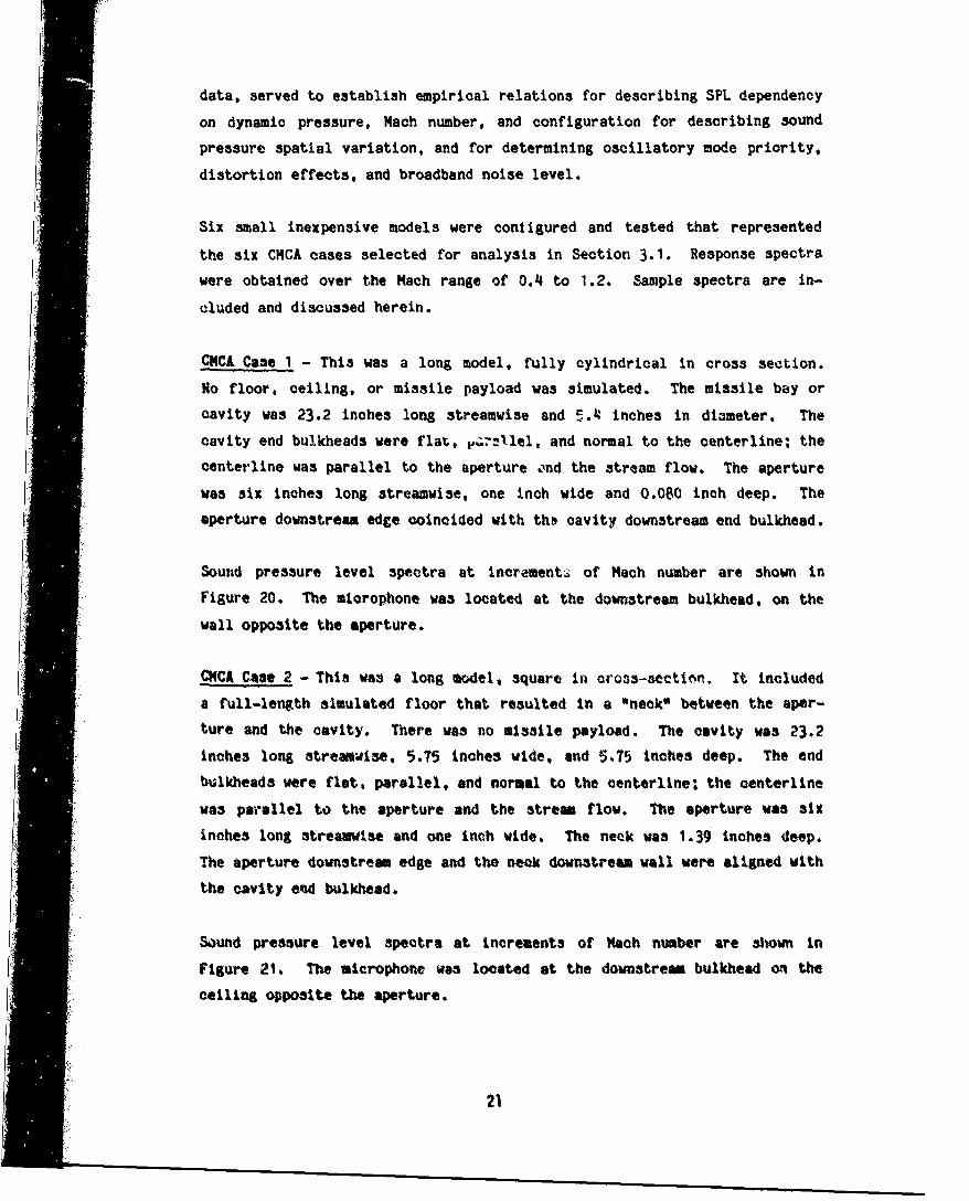
Six small inexpensive models were contigured and tested that represented
the six CMCA cases selected for analysis in Section 3.1. Response spectra
were obtained over the Mach range of 0.4 to 1.2. Sample spectra are in-
cluded and discussed herein.
CHCA Case 1 - This was a long model, fully cylindrical in cross section.
No floor, ceiling, or missile payload was simulated. The missile bay or
cavity was 23.2 inches long streamwise and 5.4 inches in diameter. The
cavity end bulkheads were flat, e and normal to the centerline; the
centerline was parallel to the aperture ond the stream flow. The aperture
was six inches long streamwise, one inch wide and 0.080 inch deep. The
aperture downstream edee coincided with the cavity downstream end bulkhead.
Sound pressure level spectra at increments of Hach number are shown in
Figure 20. The microphone was located at the downstream bulkhead, on the
wall opposite the aperture.
CHCA Case 2 - This was a long model, square in cro33-secti(n. It included
a full-length simulated floor that resulted in a "neck* between the aper-
ture and the cavity. There was no missile payload. The cavity was 23.2
inches long stremuvise, 5.75 inches wide, and 5,75 inches deep. The end
bulkheads were flat, parallel, and normal to the centerline; the centerline
Was parallel to the aperture and the streas flow. The aperture was six
inches long streamwtse and one inch wide. The neck was 1.39 inches deep.
The aperture downstream edge and the neck downstream wall were aligned with
the cavity end bulkhead.
Sound pressure level spectra at increments of Mach number are shown in
Figure 21% The microphone was located at the downstream bulkhead on the
ceiling opposite the aperture.
21
CHCA Case 3 - This model was a minimum length variation of Case 1; fully
cylindrical in cross section. No floor, ceiling, or missile payload was
simulated. The cavity was six inches long streamwise (same length as the
aperture) and 5.4 inches in diameter. In all other respects, the model
was identical to Case 1.
Sound pressure level spectra at increments of tach number are shown in
Figure 22.
CMCA Case 4 - This model was a minimum length variation of Case 2; square
in cross section, and included a full-length simulated floor that resulted
in a neck between the aperture and the cavity. There was no missile
payload. The cavity was six inches long streamwi1e (same as the aperture),
5.75 inches wide, and 5.75 inches deep. In all other respects, the model
was identical to Case 2.
Sound pressure level spectra at increments of Mach number are shown in
Figure 23.
CMCA Case 5 - This was a long model, fully cylindrical in cro-s-sectio,.
No floor, ceillng, or missile payload was simulated. The model represented
an aft-opening, rearward-ejection-launch type of missile bay. The end
opening was a skewed out through the cylinder. An elliptical aperture
resulted. The entire model W33 imersed In the flow stream. The cavity
oenterline was parallel to the stream tlow, and the plane of the aperture
was at about 20 degrees to the centerline. The Covity was 5.57 inches long
at the shortest point on the circumference of the slanted opening, and 8.47
inches at the longest point. It was 0.85 inch in diameter, with 0.080 inch
wall thickness.
Sound pressure level spe~tra at increments of Mach number are shown in
Figure 24. The microphone was located at the upstream bulkhead on the
cavity centerline.
CMCA Case 6 - This was a conventional bomb-bay type of cavity. The cross
section was rectangular, the length-to-depth "qtio was 2.0. The cavity and
22

aperture were six inches long and one inch wide. The end Dulkheads were
normal to the aperture; the aperture and opposite wall were parallel to the
stream flow. There was no missile payload.
Sound pressure level spectra at inerements of Mach number are shown in
Figure 25. The microphone was located at the downstream bulkhead on the
wall opposite the aperture certerline.
3.7 DEVELOPMENT OF PREDICTION METHODS
3.7.1 Missile Bay Oscillation Frequency
As discussed in section 3.5.1, cavity oscillation may be either the result
of a shear layer instability oscillation that exists independent of' any
acoustic resonance within the missile bay or, more likely, it way be the
result of a shear layer oscillation drivinb a missile bay acoustic reson-
ance wherein the acoustic resonance sound pressures rt&ulate or eoiitrol the
shear layer instability f'requency. Analytical rel6tions for the frequency
of twe shear layer oscillation and the frequency of tne missile bay acous-
tic resonances are discussed lu sections 3.5.1 and 3.5.3.
The frequency of the shetar layer presurc- ose.llation in teos or .. ct
number is 6iven by EquaLion (1). witerety
MC N-.25 1 "
L [M j+. 2 1 + .
The exprossiotiO (Equatlons 3 ', and b) t ot , rCunat.e rrtqency
vary Sligthtly, depending on missile bay type and/or shape. In the interest
of simplif'ying the use of these equations in predictions., it is advafntu-
geous to standaraize to a sin6.e expre.msion of the for-
N F2 42< + 1F2)
where lateral acoustic mooes have been ueblecL.ed. For rectang...r vissi.e
bay$. F N 0 , ,2. , etc.-; for c indrica. .r'd arid y;r ..
23

missile bays, F a as defined in sen't.ion 3 " for conventionai bouib
;:•dyL One L, ia.L' v ven,, r' eIzLze ' z : A , , v, D, etc., oda
integers only. Since speed of sound in the free stream, C,. , is more
readily available than speed of sound in the missile bay, C, the acoustic
resonance frequency in terms of' free-stream speec of sound is (combining
f C . . ( 1+ 2 M 2 ) 1 / 2 N Ž + ( 4/
f F). (14)2 kp X2 1.F2
• With equations C1J n 4) , the 'r~quencies of ,he shear layer pressure
oscillation and the various acoustic resonance modes in a missile bay can
be calculated and plotted as a function of Mach number on a single plot a,
was done in Figure 15. The intersections of the shear layer oscillation
curves with the acoustic resonance curves identify the possible frequencies
of oscillation, and Dhe corresponding Mach number.
iBecause C., is altitude-dependent, it becomes necessary to repeat the
entire process at every altitude of' interest. Also, there can be many
acoustic resonances available in some missile bays. As a result, the curve
plotting process and the identification of curve intersections can become
extremely burdensome. It is, therefore, advantageous to normalize the fre-
quency expressions in terms of Strouhal number and to make nertain defi-
nitions and substitutions which simplify the calculations. The modified
Rossiter equation for shear layer )scilxation in terms of Strouhal number
is: NR .25j : . .R (15)
M(1+.22M ) + 1.75
The missile bay acoustic resonance (re.ognizlng that S F=L/U and C,,U/M) In
terms of Strouhal number Is:
L (I!.•2M2)1/ 22 1/2
2M Ix ;F 2(16)
24

By definition, let (1+.2M2) 1/2 H; (17)
L LSa; x= b; (18)
x F
whrb N2 F2\1/2 (2N2+b22)1/2L - (19)
2 2
2n le (22+ b 2F2)l1/2 =G (20)
Then by substitution the modified Rossiter equation for shear layer ocillation interms of Strouhal number is:
NR-- .25NR~ (21)
SM+ 1.75
and the missile boy acoustic resonance in terms of Strouhal number Is:
s GH (22)2M
By usina equations 21 and 22, shear layer oscillation modes and acoustic
resonance modes have been calculated for a representatlive missile bay model
and are shown in Figure 26. This example is for a cylindrical missile bay
laige in. comparison to aperture length, wherein a number of intersections
occur, as denoted by encirolements. This same model was tested with and
without a fuselage floor. Strong well-defined cavity o3giilations are
identified by the data symbols and corresponding SPLs in Figures 27 and 28.
25

Il. is seen that when sustaineu cavity oscillation occurs, the measured
Strouhal number tracks the calculated acoustic mode Strouhal number, and as
speed increases the cavity oscillation snifts as the shear layer oscilla-
tion Strouhai curve comes into the proximity of different acoustic modes.
At the intersections of the Strouhal curves for shear layer oscillation and
acoustic resonance, i.e. where the two frequencies coincide,
NR . GH."" , (23)
-•-. )+ 1.75 2M.
where subscript "i" denotes intersection. by algebraic manipulation,
(H IR,2) (24)M 1,75G
"This is a useful interim form, in that the quantity (Hih)i involves only
the intersection Mach number, and the right side involves only the
dimensional and modal-order parameters relatinb to shear layer and acoustic
resonance frequencies. Since, by definition,
M 12
and by further manipulation, the intersection Hach number is
M,- .2] (26)
f rom equation 22, the Strouhal numbor where intersection occurs is:
S G (27)
26
~~~~~~~~~~~~............. ........ •.... .. •.,,-,....::...y .". .,'. .' ........ :,. ,,.'•• ....

A value of G can be calculated from Equation 20 for each acoustic resonance
mode in the missile bay, and substituted into Equation 24 to obtain a value
of (H/M)i for each intersection of the shear layer oscillation curves
(N =1,2,3, etc.) and the acoustic resonance mode curves. The values of
(H/M)i thus obtained are then substituted into Equation 26 to yield the
Mach number at which each intersection occurs. The corresponding Strouhal
number at which an intersection occurs is obtained from Equation 27. As a
convenience to aid in these calculations, values of Mi and Si may be
obtained directly from Figures 29 and 30 for Macb numbers up to 2.0, shear
layer modes up to the 5th orcier, and G values up to 4.0.
The values of Mi and Si for each potential cavity oscillatory coiidition
(each intersection) have been considered indeperndently of altitude. The
frequency in cycles per second commensurate with each intersection is
determined from
SU S.M.C GHCo.
L L 2L (28)
Values of Coo are obtained from standard atmospheric tables.
In the exploratory tests, it was observed that cavity oscillation often
began at Mach rnumbers less than Mi and as speed increased, oscillation
Icontinued beyond Mi. A study was conducted to determine the range (on
either side of the intersection Mach number) over which sustained cavity
oscillation occurred. From this study of scaled model test data, empirical
expressions were developed that defined the onset and termination of cavity
oscillation in terms of' Strouhal number and Mach number. The expressinns
are as follows, where subscript "o" denotes onset of oscillation and 't"
denotes termination:
27
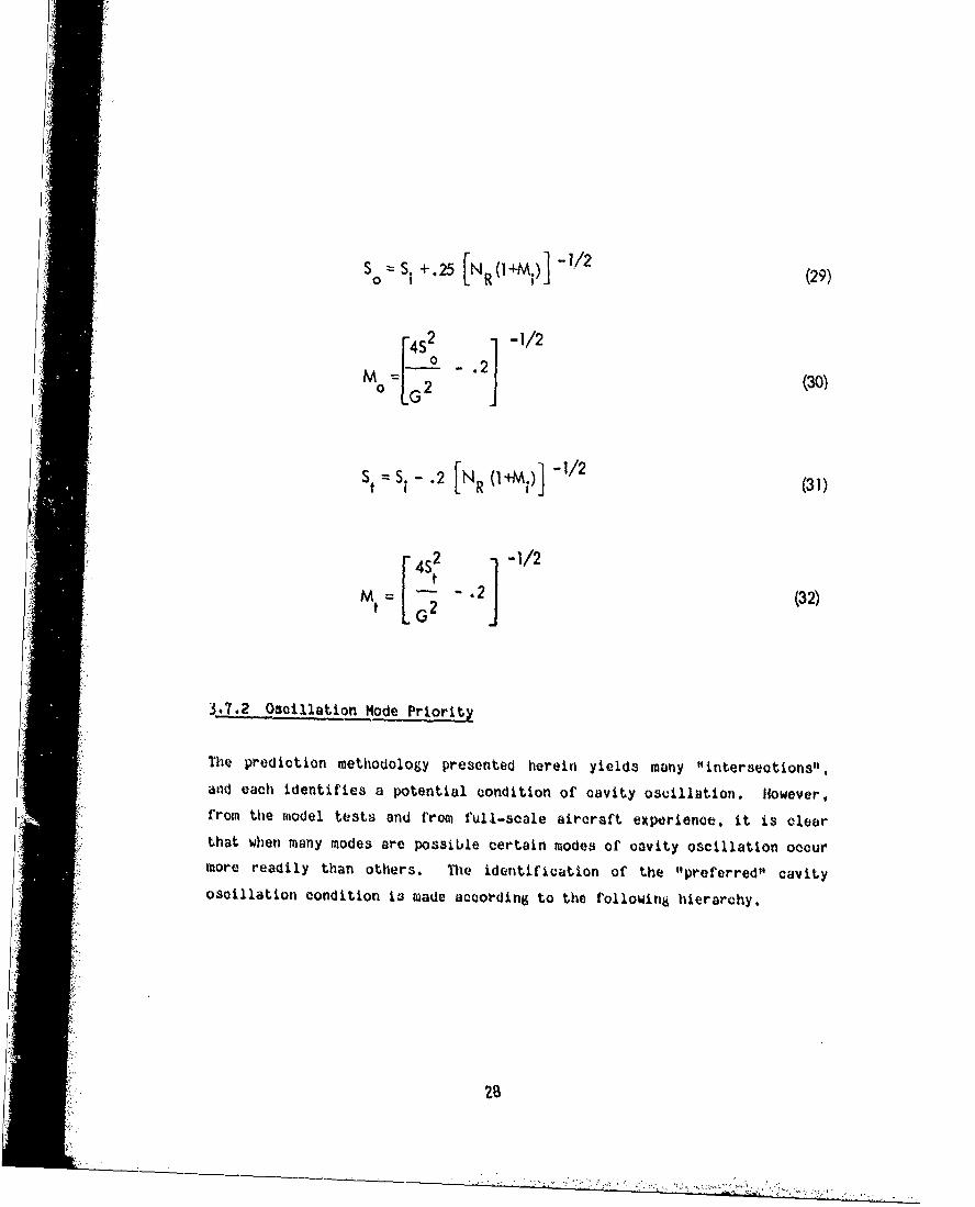
S ~S +.25 [NR(1±M. -1/2 (90 R, (29)
-4S 2 21 -1/2!.M = 0 .20 = 2 (30)
S s- .2 [NR (1 ] -1/2- (31)
42 -1/2
S-.2 (32)Mt G2
3.7.2 Oscillation Mode Priority
The prediction methodology presented herein yields many "intersections",and each identifies a potential condition of cavity oscillation. However,from the model tests and from full-scale aircraft experience, it is clearthat when many modes are possible certain modes of cavity oscillation occurmore readily than others. Die identification of the "preferred" cavityoscillation condition is made according to the following hierarchy.
i22"
......... 2B
' .,.

Shear layer pressure oscillation mode priority:
Priority Mode
A NR= 2
B NR=1
C NR=3
D NR=4
Acoustic mode priority in conventional bomb bays:
1st 0,O,Nz
2nd NXO.Nz
3rd Nx,0
Acoustic mode priority in rectangular misile bays:
"1st N ,0,tNz
2nd Nx%0,0
jrd 0,O.Nz
Acoustic mode priority in cylindrical and semicylindrical missile
bays:
lt Nw,0.0
2nd Nx ,m,n
:xamine each shear layer oscillation frequency curve for intersections with
acoustic mode curves, and assign to each intersection a letter-number
priority wherein the letter denotes shear layer mode priority and the num-
ber denotes acoustic mode priority. In those Mach ranges where more than
one intercept exists, the preferred cavity oscillation condition is the one
"of highest priority. The shear layer mode priority is btven preference
over acoustic mode priority.
29
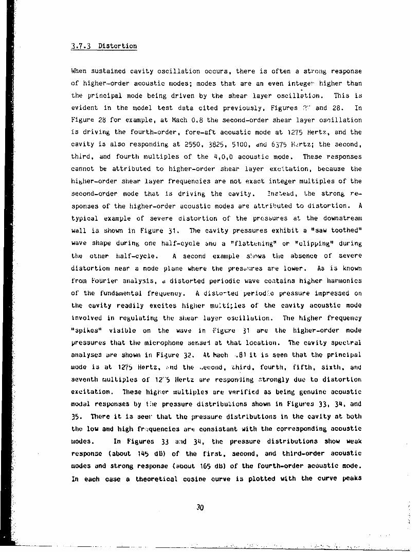
3.7.3 Distortion
When sustained cavity oscillation occurs, there is often a stro.ng response
of higher-order acoustic modes; modes that are an even integer higher than
the principal mode being driven by the shear layer oscillation. This is
evident in the model test data cited previously, Figures 2:' and 28. In
Figure 28 for example, at Mach 0.8 the second-order shear layer oscillation
is driving the fourth-order, fore-aft acoustic mode at 1275 Hertz, and the
cavity is also responding at 2550, 3825, 5100, and 6375 H-rtz; the second,
third, and fourth multiples of the 4,0,0 acoustic mode. These responses
cannot be attributed to higher-order shear layer exciltation, because the
higher-order shear layer frequencies are not exact integer multiples of the
second-order mode that is driving the cavity. !net'ead, Lhe strong re-
sponses of' the higher-order acoustic modes are attriPuted to distortion. A
typical example of severe distortion of the presbures at the downstream
wall is shown in Figure 31. The cavity pressures exhibit a "saw toothed"
wave shape during one half-cycle anu a "flattening" or "clipping" during
the otner half-cycle. A second example s!inws the absence of severe
distortion near a node plane where the pres.,,res are lower. As is known
from Fourier analysis, d distorted periodic wave contains higher harmonies
of the fundmnental frequency. A distorted period::-c pressure impressed on
the cavity readily excites higher mu.ltiles of' -the cavity acoustic mode
involved in regulating the shear layer oscillation. The higher frequency"spikes" visible on the wave in Figure 31 are the higher-order mode
pressures that the microphone se, sei at that location. The cavity spectral
analyses are shown in Figure 32. At hach ;.81 it is seen that the principal
mode is at 1275 Hertz, ,.nd the ,.ecoad, ýhird, fourth, fifth, sixth, and
seventh multiples of 12"5 Hertz are responviing -trongly due to distortion
excitation. The-se higrer multiple.s are verifif-d as being genuine acoustic
modal responses by the pressure distributions shown in Figures 33, 34, and
35. There it is seer that the pressure distributions in the cavity at both
the low and high fri:quencies art consistant with the corresponding acoustic
wodes. In Figures 33 a'id 34, the pressure distributions show weak
response (about 1I5 dB) of the first, second, and third-order acoustic
modes and strong response (Obout 165 db) of the fourth-order acoustic mode.
In each case a theoretical cosine curve is plotted with the curve peaks
30A

scaled to the maximum level of the measured data. Clearly, the trend of
each data set follows the theoretical cosine variation for the mode
represented. At 2550 Hertz, the second multiple of the principal mode, the
pressure distributions are seen in Figure 35 to agree quite well with the
eighth order cosine curve, indicating that there is, in fact, an eighth
order acoustic mode responding. At 3825 Hertz the twelfth order mode is not
verified, but neither is it refuted due to an inadequate number of survey
points. Obviously, an inordinate number of measurements would be req .ired
to identify these high multiples of the principal mode.
Distortion induced response was observed in a number of the subscale model
tests, usually when cavity sound pressure levels exceeded 155 to 160 dB and
invariably when the level exceeded 165 dB. However, resources did not
permit sufficient study to develop reliable techniques for precisely
predicting either the occurrence or level of these distortion induced
modes. As a guide, one can expect distortion-induced higher-order modes to
occur at Mach numbers above .65 when the cavity oscillation level at the
principal mode exceeds 160 db. Expect the second, third, and fourth
multiples of the principal mode to be about the same level as the principal
mode. Expect the fifth multiple and above to decrease about three db per
multiple. Generally, if levels are severe enough to result in distortion-
induced response, the levels will be intolerable and alleviation will be
required.
3.7.4 Correlations With Prior Experiments
The cavity oscillation frequency prediction methodology was applied to
conventional bomb-bay-type cavities, both deep and shallow, for which test
data were available in the literature. Some of the results of Rossiter's
work (Reference 2) are shown in Figures 36, 37, and 38 to illustrate the
coupling of shear layer modes with acoustic modes. In Figure 36, the first
five acoustic modes calculated for Rossiter's deep cavity (LID 1) are
shown as solid lines. The first six modes of the shear layer oscillation
(as given by the modified Rossister equation) are shown by dashed lines.
The solid symbols denote cavity oscillation that. Rossiter observed.
"31

The depth mode (0,0,1) is seen to be low enough to couple strongly with the
first "Rossiter" mode. When the second "Rossiter" mode coupled with the
first complex streamwise/depth acoustic mode (1,0,1) at about M = 0.9, the
first "Rossiter" mode subsided. Calculated modes and test results are
shown in Figure 37 for an intermediaie depth (L/D = 2). In this case, the
first complex acoustic mode (1,0,1) coupled with the third "Rossiter" mode
near M = 0.55, and with the second "Rossiter" [node near M = 0.8. Note
also that concurrent with the coupled shear layer/acoustic mode oscilla-
tion, there was pure shear layer oscillation as indicated by the open
symbols. In Figure 38, which is for a very shallow cavity (L/D = 8), the
first depthwise acoustic resonance frequency was so high it was completely
out of consideration for shear layer coupling. Only the first two fore-aft
acoustic modes are within the range of interest, and there was no evidence
of coupling of the shear layer oscillation with these acoustic modes.
here, only pure shear layer oscillation occurred. It is also interesting
that, in the L/D = 8 case, Rossiter's data showed that where there was no
apparent acoustical coupling, the sound pressure level was significantly
reduced from the SPL produced in the deeper cavities. This was true de-
spite the fact that, with decreasing cavity depth, the transducer used to
measure sound pressures was located inherently closer to the oscillating
shear layer.
3.7.5 Sound Pressure Level Prediction
Sound pressure 'evel prediction methods were developed empirically from the
test results for 10 subsoale models that were tested with variations on
aperture position ana neck length. The oscillatory sound pressure levels
were normalized to dynamic pressure, q, and plotted against Mach number for
each test as illustrated in the composite plot in Figure 39. "Best-fit"
curves were constructed through the maxima on 3uoh composite plots. These
best-fit curves were then grouped together according to type of missile bay
configuration such as cylindrical enclosed, rectangular enclosed, and
rectangular with one wall open. Straight-line envelopes were fitted to
these groups of best-fit curves and are shown in Figures 40, 4~1, and 42.
Such envelopes were arranged to reflect conservative estimates of the
normalized fluctuating pressure level; they are conservative in that most
32
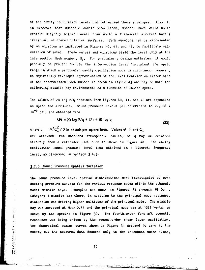
of the cavity oscillation levels did not exceed these envelopes. Also, it
is expected that subscale models with clean, smooth, hard walls would
exhibit slightly higher levels than would a full-scale aircraft having
irregular, cluttered interior surfaces. Each envelope can be represented
by an equation as indicated in Figures 40, 41, and 42, to facilitate cal-
culation of level. These curves and equations yield the level only at the
intersection Mach number, Mi. For preliminary de~i~n estimates, it would
probably be prudent to use the intersection level throughout the speed
range in which a particular cavity oscillatiun mode is sustained. However,
an empirically developed approximation of the level behavior on either side
of the intersection Mach number is shown in Figure 43 and may be used for
estimating missile bay environments as a function of launch speed.
The values of 20 log P/q obtained from Figures 40, 41, and 42 are dependent
on speed and altitude. Sound pressure levels (dB referenced to 2.9006 x
10-9 psi) are obtained from
SPL - 20 log P/q + 171 + 20 Iog q (33)
"whe-e M2C. / 2 in poinds per squore inch. Volues oF P and C.
are obtained from standard atmospheric tables, or q may ue obiýained
directly from a reference plot such as shown in Fiture 414. The cavity
oscillation sound pressure level thus obtained is a discrete frequency
level, a3 discussed in section 3,4.3.
3.7.6 Sound Pressure Spatial Variaticn
The sound pressure level spatial distributions were investigated by con-
ducting pressure surveys for the various response modes within the subsoale
model missile bays. Examples are shown in Figures 33 through 35 for a
Category 1 missile bay where, in addition to the principal mode response,
distortion was driving higher multiples of the principal mode. The missile
bay was surveyed at Mach 0.81 and the principal mode was at 1275 Hertz, as
shown by the spectra in Figure 32. The fourth-order fore-aft acoustic
resonance was being driven by the second-order shear layer oscillation.
The theoretical cosine curves shown in Figure 34 descend to zero at the
nodes, but the measured data descend only to tie broadband noise floor,
33
w •" t" : -" .. . S. , • •: - : ..| . .. •"l - .' -"•• ;'"• '" ••i:' L'" •
which averages around 135 dB in the 25 Hertz analysis bandwidth. The
broadband noise also adds to the level of the oscillation to some extent on
either side of the mcde,:. This has the effect of flattening the sound
pressure distribution curve.
In Figure 28, a different oscillatory condition is seen at Mach 0.71.
There, the second-order shear layer oscillation is driving the third-order
fore-aft acoustic resonance. The spectrum analysis in Figure 32 shows this
principal mode to be at 975 hertz. A. was the case at Mach 0.81, the
spectrum. analysiz also shows strong respon.ie at a higher multiple of the
principal mode, in this case 1-350 Hertz, twice the principal mode fre-
quency. Sound pressure surveys .f thL !iach 0,71 nsci, Iatory cot-dition are
shown in Figures 45 through 48. The first- and second-order fore-aft
acoustic modes are shown in Figure 45 to be responding weakly (about 145 dB
maximum). The principal mode (3,0,0 responding at atout 165 UL maximum) is
shown in Figure 46, along with weak response %.aboot 145 _ib maximum) of the
(4,0,0) mode. The measured frequencies are accurate to 1 12.5 Hertz (since
the analysis bandwidth in this case was 25 Hertz) and agree very well with
the calculated frequencies shown in Figure 26. The olcvlated frequencies
for the 2,1,0 and the 5,0.0 modes are nearly equal (1580 and 1588 Hertz re-
spectfully from Figure 26) and both, though weak at 145 dB maxmlum, are
discernible in the Figure 47 survey for 1600 Hertz. The 3,1,0 mode cal-
culated to be 1731 Hertz is weak, but also evident in tlie Figure 47 survey
for 1775 Hertz. The Figure 48 survey for 1950 Hertz is most interosting.
It clearly shows strong response (159 d13 maximum) of a fourttl-order fore-
aft acoustic mode. However, thu pure fourth-order fore-aft mode would be
expected at about 1300 Hertz, not 1950. This is seen in Figure 26 to be
the 4,1,0 mode which was calculated as 1923 Hertz. T'his response frequency
is the second multiple of' the principal mode, evidenced by the Figure 32spectra, but note in Figure 28 that neither of the "No5siter" curves coin-
cide with this response mode. This response is induced by disLtortion atthe 975 hertz frequency. However, in this instance, the distortion excites
a complex mode, the 4,1,0, rather than the 6,.0,0, the second multiple ofthe principal mode. A final pressure ditstribution survey is shown in
Figure 48 for the 7,0,0 mode responding at 2250 Hertz. The 7,0,0 mode,
which has 7 minima and 8 maxima, is weak (about 144 dbi) but is still
discernible.
34
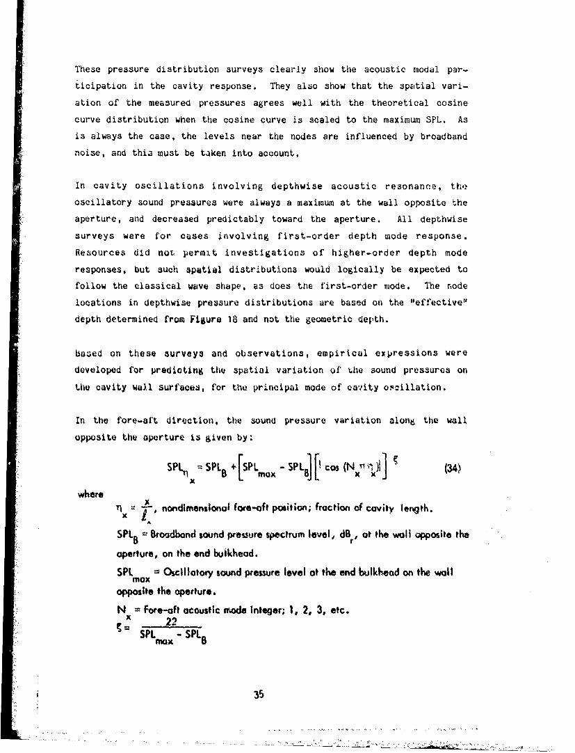
These pressure distribution surveys clearly show the acoustic modal par-
ticipation in the cavity response. They also show that the spatial vari-
ation of the measured pressures agrees well with the theoretical cosine
curve distribution when the cosine curve is scaled to the maximum SPL. As
is always the case, the levels near the nodes are influenced by broadband
noise, and this must be taken into account.
In cavity oscillations involving depthwise acoustic resonance, the
oscillatory sound pressures were always a maximum at the wall opposite the
"aperture, and decreased predictably toward the aperture. All depthwise
surveys were for cases involving first-order depth mode response.
Resources did not permit investigations of higher-order depth mode
responses, but such spatial distributions would logically be expected to
follow the classical wave shape, as does the first-order mode. The node
locations in depthwise pressure distributions are based on the "effective"
depth determined from Figure 18 and not the geometric depth.
based on these surveys and observations, empirical expressions were
developed for predicting the spatial variation of the sound pressures on
the cavity wall surfaces, for the principal mode of cavity os.illation.
In the fore-aft direction, the sound pressure variation alone the wall
opposite the aperture is given by:
SPL'n = SPL~ +.[SPL - SP 1.8] co1](N (34)x
wherer J j-. nondimensionol fore-oft position; fraction of cavity length.
SPLB Broadband sound pressure spectrum level, dBr, at the wall apposite the
aperture, on the end buikhead.
SPLax c Oscillatory sound pressure level ot the end bulkhead on the wall
opposite the operture.
N = fore-aft acoustic Pmode Integer; 1, 2, 3, etc.g= 22
SPLm - SPL8
35

Equation 34 is valid for any enclosed rectangular, cylindrical, and s'ými-
cylindrieal wissile bay and for conventional bomb bays. For pure fore-aft
modes (no depth mode response) the fore-aft pressure variation is the same
at any depth, but Lhe broadband level used in the equation must be for the
applicable depth. Fore-aft sound pressure distributions were calculated
using Equation 34 for comparison with the theoretical cosire curve and to
show the limiting effect of the broadband noise. The comparison is shown
in Figure 49. The two cases considered are the principal modes of response
in the 21-inch-long cylindrical missile bay at Mach 0.71 and 0.81.
In the deptnwise direction, the qouod pressure variation on the end
bulkhead in endlosed rectangular alisile bays is given by the same
expreision, with the subscrJpts redefined to denoto the depth directions,
e.g.:
SPL• = SPL + [SPL - SPLO] [!Cos (N (35)a' I Max L z
z
nondiw-ensionol Mepthwise oosition; fraction of cavity depth.z
N depth c_,:ovf;•. mode integer; 1, 2, 3, ewc.z
SPLB b= woodbond sound p'essui% level, d r, at •tr z
In conventional botb-bay cavities, the depthwise sound pressure variation
"at the etW bulkhead i1 given by:
NzJ(-iz) 1]
6 1OSspyz- + SL -P Co. (36)
-where IS2z
N depth acoustic mode integer; I, 3, 5, 7, etc.
ýor pure depth modes (no fore-aft. .ode response), the depthwise pressure
variations gIiven by Equations 3ý and 36 are the same at any fore-aft
position in the missile bay, but the broadbana noise level used in the
equations must be for t=•e proper depth and fore-aft position.
S. • • •' ... 'f: ,. ,-.,)..': : !,,., ,, "" , : :c]•,:',,'., -,-•:.:-.• ,... •,,.

The expressions for depthwise SPL variation in enclosed cylindrical and
semi-cylindrical missile bays are more complex and were not developed,
because the principal response mode in such missile bays will rarely
involve tangential and radial modes. The radial frequencies are too high
to be driven by the probable shear layer oscillation. The tangential modes
are highly damped and will normally not be excited.
When the cavity oscillation involves combined fore-aft and depth mode re-
sponse (complex modes), the pressure variation at the surface will still be
as given by Equations 34, 35, and 36. However, to obtain pressure varia-
tions at points within the interior volume (away from the surfaces), the
fore-aft and depth mode equations must be combined. While not overly
difficult, the equations are cumbersome and were not developed here, since
the level of a complex mode at any "interior" point in j cavity will always
be less than the level near the suri'ace. In preliminary analyses, the max-
imum levels should be of primary concern. An illustration of complex mode
pressure variation within an enclosure can be found in Reference 20.
3.7.7 Broadband Noise
In the subsoale model test., it was observed that the broadband noise level
did not vary substantially among missile-bay categories one, two. and four.
Pie uingle most important parameter was microphone location relative to the
aperture downstream tege. Nermalized broadband noise level noar the down-
stream edge of the aparture is shown in Figure 50 as a function of Strouhal
number, where the characteristic dimension is the aperture length. Forlocations pore remote 'row the aperture, the broadband nolse levels vill be
lower. To account for this, Figure 51 was constructed from the test d~ta
to permit empirical corrections of thea •igure 50 level3.
.- j'adband noise data were obtained from spectrum analyses for each missile-
bay =moel tested. I4wuver, when normalized to dynamie pressure and plotted
as a function of Strouhal number, the data did not collapse to a single
band or cluater. The implioation is that broadband level in the cavity is
not directly dependent on q. InStead, the level at low lich number is
higher than the dynamic pressure warrants and is being influenced by other
37

sources such as upstream flow noise, valve noise, etc., or, at the high
Mach numbers the subscale models and flow facility provided unusually clean
flow at the aperture that resulted in low broadband noise in the missile
bay. A comparison with published data for full-scale dircraft and 7or wind
tunnel tests of subscale models revealed that the published broadband noise
levels generally equaled or exceeded the levels measured here. This raised
the suspicion that the published data might also b. contaminated by
extraneous sources, which is not unlikely when one recognizes that the wind
tunnels and the full-scale aircraft both involve intense extraneous sources
that could radiate noise into the cavity. This suspicion precluded the use
here of the published broadband noise data, since Lne objective is to
predict the broadband noise level due solely to the flow over, or into, the
cavity. (The user must "add in" the extraneous noise from his particular
engines, airframe structure, aperture doors, etc. to arrive at the most
-* realistic prediction of his environment.) The presently measured broadband
noise levels are therefore presented and are considered adequate since the
* broadband noise is of seuondary importance compared to the discrete levels
that exist during cavity oscillation.
3.7.8 Clutter Effecte
A full complement of cruise missiles could be expected to displace as much
as one-half of the air in the missile bay, or block up to one-nalf of the
cross sectional area, depending on the configuration. The missiles might
al]3o be expected to disperse the sound waves and decrease the strength of
the sound pressures at resonance. A missile positioned over the aperture
might be expected to decrease the efficiency of the shear layer excitation
of the cavity acoustic resonances. However, experimental investigations did
not always substantiate these expectations.
The photo in Figure 52 illustrates an extreme case of clutter in a short,
rectangular missile bay model. The sound pressure spectra in Figure 52
show the effect of the missiles on oscillatory response. The SPL is de-
creased about 5 dB, and the response frequency is decreased about 13 per-
cent. In Figure 53, the photo illustrates the case of miss8ies positioned
very near the aperture but not interfering with the flow. The companion
38
response sp.,ctra show a 10 !iB reduction in SPL and a 10 percent reduction
in oscillatory frequency.
The reduction in frequency is consistent with Parker's observations
(Reference 21) in his experiments related to acoustic resonances in heat
exchangers. The presence of the clutter (missiles) reduces the speed of
sound in the missile bay, thus reducing the acoustic mode frequencies. The
reduction in sound pressure level is attributable to scattering and
damping.
These effects on SPL and frequency are significant. The frequency change
is particularly important, since a lower frequency can result in a lower
speed (Mach number) at which the oscillation occurs. Whether or not
oscillation will occur at any given speed is, therefore, influenced by the
missile payload on board. In a CMCA, the significance of clutter and/or
partial blockage will depend on the configuration. However, the
determination of clutter effects is best done experimentally during the de-
tailed design phiase.
39
3.8 CAVITY OSCILLATION PREDICTIONS FOR SELECTED CRUISE MISSILE CARRIER
AIRCRAFT (CMCA)
3.8.1 CMCA Cases
Six CMCA cases were selected for analysis, as discussed in Section 3.1.
The general arrangement of the missile bays, and the pertinent descriptive
data are shown for each case in Figures 2 through 4. Since the prediction
methods provide the means for analyzing cavity oscillation at any desired
temperature/altitude/speed/dynamic pressure conditions, the six CMCA cases
were analyzed for typical conditions to provide comparative data and a
demonstration of the methods. The analyses and the conditions applied were
as follows:
o Determine the speeds at which each missile-bay oscillation condi-
tion occurs and determine the frequency and SPL of the oscillation.
Do this for 25,000 feet altitude, standard atmosphere, for speeds
ranging from M20.4 to 1.0.
o At nominal launch conditions of Mach 0.8 at 25,000 feet, determine
the missile-bay oscillatory frequencies and corresponding SPL's,
and the broadband noise level, to obtain a sound pressure spectrum
at a representative location. Determine sound pressure spatial
variation.
o at a second launch condition of Mach 0.8 at 37,000 feet, determine
the missile-bay o~ciliation frequencies and corresponding SPL's.
o Assume that the missile bay is empty; there are no baffles or
partitions in the launchers or missile bays; and neglect the
effects of aperture doors.
40

3.8.2 Sample Application of Prediction Procedures
In the interest of clarity and for illustration, a rather elementary step-
by-step application of the cavity oscillation prediction procedure follows
for CMCA Analysis Case 2. Because of the geometry of Case 2, many modes
are possible. While this makes it more burdensome to analyze, it is a com-
prehensive example; thus its selection.
missile bay: x = 100 feet; 1y = 16 feet; iz 9 feet
aperture/neck: Lx = 26 feet; Lz = 6 feet; Ly 6 feet
Geometry:
1. Case 2 constitutes a long, rectangular cross-section cavity exposed
to parallel stream flow, via a well-defined neck. Dimensions are:
Frequency Calculations:
2. Calculate values of H using Equation 17, at Mach increments of 0.1M
for the speed range of interest, e.g.,
M . .5 .6 .7 .8 .9 1.0 1.1 1.2
H 11.0161 1.025 11.035 11.048 1 .062 1 1078 1 1.095 1.114 11.135
3. Calculate values of shear layer oscillation Strouhal number at each
Mach number increment for each shear layer mode through NR=5, using
Equation 15 and the values of M and H established from Step 2,
e.g.,
Mach 0 .4 .5 .6 .7 .8 .9 1.0 1.1 1.2
N =1 .348 .332 .316 .302 .288 .276 .264 .252 .241
N =2 .812 .774 .738 .705 .673 .643 .615 .588 .562e
N -3 1.276 1.216 1.160 1.108 1.058 1.011 .967 .924 .884e
N =4 1.739 1.658 1.582 1.510 1.442 1.379 1.318 1.260 1.205e
Ne=5 2.203 2.100 2.003 1.913 1.827 1.746 1.670 1.596 1.526
41
Si•, ,. • ' . . .. . . . ,, : ,• .... , , " , " . ', • :';,. • • ' '.. , . .. • , ,•:.•i):, . : ,•. ,..,M '

4. Construct a "master" plot (that can be copied and used repeatedly)
of shear layer oscillation Strouhal number versus Mach number using
the values tabulated in Step 3, e.g., see Figure 54.
5. Calculate values of G using Equation 20. Use the appropriate de-
finition of F consistant with the missile bay cross-section. (See
Section 3.7.1 or the list of definitions/symbols). Tabulate G for
each fore-aft acoustic mode through NxZ10, each depthwise acousti'c
mode through Nz=2, and each complex acoustic mode through
Nx=2,N =2, e.g.:
N 1 2 3 4 5 6 7 18 9 10 0 I1 2 0 1 2
F 0 0 0 0 0 0 0 0 0 i0 1 I1 1 2 12 2
G .26 .32 .78 1.04 1.3 1.56 1.82 2.08 2.34 2.60 2.2.90 2.94 5.78 5.78 5.80
6. For each acoustic mode order calculate values of acoustic mode
Strouhal number at each Mach number increment. Use the values of H
and G tabulated in Steps 2 and 5, with Equation 22, e.g.:
Moch No, .4 .5 .6 .7 .8 .9 1.0 1.1 1.2
NX=I, NX-) .330 .266 ,224 .195 .173 .156 .142 .132 .123
NX,2, N ,0 .660 .533 .448 .389 .345 .311 .295 .263 .246
N -3, N -0 .991 .799 .673 .584 .518 .467 .427 .395 .369
N -4, N ,0 1.321 1.066 .897 .779 .690 .623 .569 .427 .492X
N NX, N ,0 1.651 1.332 1.121 .973 .663 .779 .712 .658 .615
N *6, N w0 1.981 1.599 1.345 1,168 1.035 .934 .A54 .790 .738
N 47, N -0 2.311 1.865 1.570 1.362 1.208 1,090 .996 .922 .861
N -8, N D0 2.642 2.132 1.794 1.557 .,381 1.246 1.139 1.053 .9M4
N -9, N 10 2.972 2.39 2.018 1.752 1.5,3 1.401 1.281 1.185 1.107
N =I0, N -0 3.302 2.665 2.242 1.946 1.726 1.557 1.423 1.317 1.230
N N,0, N ,I 3.670 2.962 2.493 2.163 1.910 1.731 1.582 1.463 1.367
N N-l, N-I. 3.60' 2.972 2.501 2.17" 1.925 1.737 1.586 1,466 1,371
N 02, N 01 3.734 3.013 2.536 2.201 1.951 1.761 1.610 1.489 1.390
N -0, N w2 7.341 5.924 4.9f8 4.327 3.836 3.462 3.115 2.927 2.733
N *l, N ,2 7.341 5.924 4.985 4.327 3.836 3.462 3.165 2.927 2.733
N-2, N -2 7.366 5.94 5.002 4.342 3.050 3.474 376 2.937 2.74.3
42

7. Plot the values of Strouhal number computed in Step 6 on a copy of
the plot of shear layer oscillation Strouhal numbers constructed in
Step 4. Identify or note the approximate intersections of the
shear layer mode curves and the acoustic mode curves, (see Figure
55). Each intersection defines a potential cavity oscillation
mode.
8. From among the intersections noted in Step 7, list the more
probable cavity oscillation modes using the shear layer/acoustic
mode hierarchy discussed in Section 3.7.2, e.g.:
Mach Range Probable Oscillation Mode Priority
(NR) (Nx, Nz)
M .4 NR=I, Nx=1, Nz=0 B2
-4 to-.7 - N ;3 7 t'H4, N =0 C-R X z
.4 to .7 NR=2 , Nx=3, Nz=0 A2
t - N.R = 1 •,-•,-N =0 . 2-
.7 to 1.0 NR=2 , N =4, N =0 A2
.7 to 1.0 NR=3, Nx=6, N =0 C2
o -t*o- --- - g =7, f+ %0 C2
M a 1.0 NR=2, Nx=5, Nz=0 A2
MZ 1.0 NR NX=2, N z0 B2
M k .0 N&- N4NX-6, N1r 42
Note that at any speed range there are ample modes available having
A, B, or C priority, and in this case it is unnecessury to list the
D priority modes. Identify one or two top-priority modes in each
range and rule out all others, e.g., the dashed lines.
The application of the mode hierarchy rules to select the probable
modes can be deferred until Step 11 if preferred, where a graphical
presentation of the intersections will be available and all of the
prevailing conditions can be visualized. However, doing so in this
step reduces the mount of calculation in Step 9.
43

9. Compute and tabulate the Mach numbers and Strouhal numbers of
onset, intersection, and termination for each of the probable
cavity oscillation modes identified in Step 8, using the equations
below which were obtained from Section 3.7.1:
IHN N N G (-M. M. S. S S M M
R Z , I I 0 o t
1 1 0 .26 2.73 .372 .355 .568 .184 .230 .745
1 2 0 .52 1.08 1.021 .280 .456 .139 .590 3.414
2 3 0 .78 1.99 .515 .776 .920 .661 .432 .612
2 4 0 1.04 1.35 .784 .702 .834 .596 .649 .948
2 5 0 1.3 .97 1.166 .631 .751 .535 .939 1.447
3 6 0 1.56 1.44 .729 1.120 1.230 1.032 .661 .803
G N +b2F 2 calculated in step 5.
2 (NR .25) -G
1.75G
[It)2 1-1/2 IHM.- -. 2] S.=Ll I J M I
. - 25 NR (I +M /2 St = -2 [N ( +M -2
S 4o 0 1 1/2 -4S 2 1-2VM 0 .2- Mt = - .2
G2 L2
44
.1-.,.,t* .

10. Using the plot prepared in Step 7, and the values of Mo, M1t and tt
computed in Step 9, indicate the speed range over which each pro-
bable mode would respond, as shown by the shading in Figure 56.
11. Inspect Figure 56, apply the cavity oscillation mode hierarchy de-scribed in Section 3.7.2, and conclude the following: Priority Aand B modes are available throughout the speed range; therefore,
rule out all others. The cavity oscillation modes predicted are
the (2)(3,0), the (2)(4,0), the (2)(5,0), the (1)(1,0), and the
(1)(2,0).
12. Compute the cavity oscillation frequencies using Equation (28),
f=S MAC, /L, where C. is obtained from reference tables to be 1016ft/sec at 25,000 ft, and 968 ft/sec at 37,000 ft. Obtain the
following:
Frequency FrequncyMO& Onset Interectlon Termnnation @25000 Ft @ 37000 Ft(N&(N',L ) Mach Moch Mach Hertz Heft
(2)3,0) .432 .315 .612 15.6 14.9
(2)(4,0) .649 .784 .9" 21.5 20.5
(2)0•0) .9039 1.166 1.447 28.7 27.3
(1)(1,0) .23D 372 .745 5.2 5.0
(I)(2.0) .590 1.021 3.414 11.2 10.7
Sound Pressure Level Derivations,
13. Enter Figure 41 at the interseotion Mach number for each cavityoscillation mode (or use tho equations noted on Figure 41) and
obtain the normalized maximum sound pressure levels at intersection
as follows:
MO"e Intvrectlen 20 ooqPAq(N0(N', Nt) Mach
(2)0.) .StS -2D.7
(•)(4.0) .704 -2.
C2)C5.0) 1.166 -26.4
(1)(110) V32 -19.6
MUM2.0 1.021 -25.1
45

14. Determine dynamic pressure q (in pounds per square inch) at each
r3•• intersection Mach number for the desired altitude of 25000 feet,
and convert normalized sound pressure level (20 log P/q) to SPL for
each mode, as f6llows:
SPL= 20 log P/q +20 log q U170.75
I=M2 -P obtain P C fromi reference tables
2
Mode Intersection q (PSI) SPI (dB)( (R)N, Nz) Mach @ 25,000 Ft @ 25,000 Ft
(2) (3,0) .515 1.01 150(2) (4,0) .784 2.35 155(2) (5,0) 1.166 5.19 159(1) (1,0) .372 .53 146(1) (2,0) 1.021 3.98 158
15. To calculate SPL for each cavity oscillation mode, at spetds both
below and above intersection, use Figure 43 to obtain the correc-
tion to be applied to the intersection SPL. For convenience enter
Figure 43 at five speeds, whereby Ad8 is.
M g M~2 IN0 2 T Mt
---
Ade -7 -2 0 -2 -10
46

Using SPL@M SPL@M! + AdB, and disregarding Mach numbers that arewell below .4 and above 1.2, the resulting sound presure levels are:
Mode Mach SPL@25K ft Mode Mach SPL .)25K ft(NR)(Nx, N.) Nuer (NR)(N., N.) Nunbr
(2)(3,0) M .432 143 (1)(10) M
0St14 .301
2 •2
Me - .515 150 . .372 146
M+Mt = .563 148 M1+M .558 144
2 2
M = .612 140 Mt = .745 136
(2)(4,0) MW .649 148 (1)(2,0) M - .590 151
Mý4#A .716 153 A4 0 805 1560 0
2 2
W1 -. 784 155 We. a1.021 158
MI$A8t - .66 153 Mi4Mt 0 2.217
2 2
Mt - .948 145 Mt -3.414
(010.) M 0 -. 939 152
2We1 -I.166 159
MtM40 1.306
2
16. Plot the maximum SPL's obtained in Step 15 versus Hach number, to
obtain a graphical summary of oscillatory levels at any launch
speed at. 25000 reet altitude, as shown in Figure 57. If" desired,
the levels may be combined to obtain an envelope of overall
oscillatory level ver3us launch speed, neglecting broadband noise.
Recall that the frequencies were determined in Step 12.
47
-... . ' • • z":• .-

17. To obtain the oscillatory SPL's versus launch speed at any other
altitude, such as 37,000 feet, the levels obtained in Step 15 are
adjusted according to the change in q:
SP1 3 7 0 0 0 =SPL25 + 20 LOG( q37,000_ SPL 48 B'3,0 500q25,000- SP25,000- .8d
Environment at Selected Launch Speed of .8M; 25,000 Feet Altitude:
18. From Step 12, or from Figure 57 obtained in Step 16, determine for
.AM at 25,000 feet, that the missile bay will respond in two modes:
the ( 2 )(4,0) and the (1)(2,0). The frequency of these two modes
will vary slightly from the frequencies at the intersection Mach
numbers. Obtain frequency at 0.81 using Equation 28 and G from
Step 9:
(1.04) (1016) 2f(2) (4,0)= (2)(26)- (1' "2 2" z
(52)(1016) 8 /'=(1) (20 ) (216)= (1+.2 z0. = 10.8 Hz(1).. •(2#0)-()26
19. From Figure 57 derived in Step 16, determine the spatial maximum
sound pressure level at O.68 for the 10.8 Hertz mode to be 156 d8,
and for the 21.6 Hertz mode to be 154.5 d6.
20. Determine normalized broadband souni pressure level (1/3-octave-
band level) for each mode frequency from Figure 50. For the 10.8
Hertz mode, enter Figure 50 at S = fL/C,0 = 0.34 and read
20 log P/q -40dB. For the 21.6-Hertz mode, S=.69 and
20 log P/q t -38dB. These levels are at the downstream wall near
the aperture.
48

21. Obtain 1/3-octave broadband sound pressure level, SPLB, from the
normalized level using
SPL = 20 LOG / + 20 LOG q + 170.75B q
At .8M and 25000 ft, q = 2.44 and SPLB at 21.6 Hertz is 140.5dB.
At 10.8 Hertz it is 138.5 dB.
22. Convert the 1/3-octave broadband noise level to spectrum level, dBr
using
spectrum SPL 1/3 octave SPL - 10 log (1/3 octave BW)
Obtain the following:
Frequency 1/3 Octave 1/3 Octave SpectrumHertz SPL - dB BW - Hz SPL- dBr
10.8 138.5 2.2 135
21.6 140.5 4.4 134
23. Determine the broadband noise level at the wall opposite the
aperture using Figure 51. Enter Figure 51 at z/L 15/26 0.58;
obtain a correction of d8= -13. Levels along the opposite wall
are therefore 13 d8 less than at the downstream wall near the
aperture, whereby at 10.8 Hertz, opposite-wall spectrum level is
122 dBr, and at 21.6 Hertz it is 121 dB r Repeat Steps 20,21,22,
and 23 at any other frequencies desired.
24. Construct a cavity response spectrum plot to summarize levels at
.814, 25,000 ft., using t'-equeneies and levels available from Steps
18, 19, and 23. The result is Shown in Figure 58. To obtain the
spectrum plot for any other altitude (at 0.81) , adjust the oscil-
latory levels and the broadband levels to account for change in q
a3 done in Step 17.
ll49

25. Determine the spatial variation of the oscillatory sound pressure
levels along the missile-bay wall opposite the aperture using
Equation 34.
22
SPI ~SPO + 1 PL .. SPý Cos NT SPI T1 SP18~ 5 max x x
Obtain SPL. fran Stop 23, obtain SPL fram Stop 19, obtain N from Step 18,max
whereby for the 10.8 Hertz mode,
.645
SP x =~ 122 +34[ Co 2nT1x]
X
and fw, the 21.6 Hart'z mode,
r .658SP Ln 121 +33.5 Ca 41r1I1n
x 1Calculate the following Ievets at the qptai! locations indicated:
( t * ) ( N N ) H ." . ' 1 --31.2 1 .5 .6 ,-
(1)(210) 10. 6 156 U5 U3* Is" 1 152 138 136 152 156
15,4
Q2) (A0) 41. ISA.5 136 1f5 I -so S 1341 154.,s. 136 1150 ISO 136 154.S
Ac~po~imo Z*1 15 IS 52 MISO 5 IS2 ISB '52 150 150 152 ISO
26. construct a plot of level verSUi spatial posiLtion alQor•.• the missile
bay ii.al opposite the aperture !.o summarize the cmvity envirotwent
at .6m, ,0ooo feet, using the valuea obtaine4 in Steps 23 and 25.
The result is shown in Figure 59.
50

3.8.3 Results of Predictions
The cavity oscillation prediction procedure, as applied to CMCA Case 2 and
described in the previous section, was used to analyze CMCA Cases 1,3,4,
and 6 (see Figures 2, 3, and 4) in accord with the conditions noted in
Section 3.8.1. Case 5 was not analyzed due to the absence of any sustained
oscillation in either the exploratory tests or the CMCA model tests
discussed in Section 3.6. A summary of the predicted oscillatory
conditions that could occur at 25,000 feet is shown in Figure 60 for each
CMCA case. The Mach number at which each oscillation begins (onset),
maximizes (intersection), and ends (termination) is tabulated along with
the maximum sound pressure levels and corresponding frequencies.
A summary of the oscillatory modes and their levels and frequencies for
launch at Mach 0.8, 25,000 feet and for launch at Mach 0.8, 37,000 feet isshown in Figure 61 for each CMCA case. The predicted spatial variations of
the SPL's for launch at Mach 0.8 at 25,000 feet are shown in Figures 62
through 66 for each case.
3.8.4 Required Alleviation
It can be seen In Figure 60 that maximum oscillatory levels at 25,000 feet
exceed 150 dB in all cases. These oscillatlons are essentially discrete
frequency pressure fluctuations that could have a pronounced effect on air-
craft integrity, depending on how closely the oscillation fr'equencies match
the airframe structural resonance frequencies. For this program, it was
presumed that the predicted levels would be intolerable and that allevia-
tion devices would be required for all cases analyzed.
S3.8. Effeetiveness of klleviation Devices
As diScussed earlier, cavity oscillations in CHCA's involve two basic
physical phenomena: shear layer oscillation and missile bay acoustic
resonances. In some very shallow cavities, the potential for missile bay
acoustic modes is severely limited and the shear layer oscillation appears
capable of sustaining itself at moderate levels Independent of acoustic
modes. Also, it is impractical to eliminate acoustic modes in an en-
51
.......................................,-..." .......... ..................'-• "'-• . . ....... • -••- '•'•' .... •-" ... ::•: ':: . . . • ,".. . . . . . . . . . . .I.. . . . .-. .,.. . . . . .,.. . .... •-;

closure. Thus,, the shear-layer oscillation is the phenomenon that is best
altered to achieve cavity noise suppression. The approach to the sup-
pression of cavity oscillation in CMCA's is, thus, similar to the approach
used heretofore on conventional bomb bays. The shear-layer oscillation
frequency is characterized by the aperture length in the streamwise
direction and the freestream velocity. With these quantities known, the
frequencies of potential oscillation can be obtained from the modified
Rossiter equation, but very little information about the physical aspects
of the coupling with acoustic resonances is available. Based on flow ob-
servations using oil streaks, shadowgraphs, and water tables, some in-
vestigators have surmised that the introduction of turbulence into the
shear layer could effectively destroy the shear layer and, therefore,
suppress cavity oscillations. The thickness of the shear layer is in-
creased by turbulence, and in some cases cavity oscillation sound pressure
levels a:'e reduced. Solid and porous spoilers, leading- and trailing-edge
airfoils and ramps, and combinations thereof have been used for suppression
devices on bomb-bay-type cavities with various degrees of success.
Cursory CMCA model tests were conducted to evaluate turbulence generating
devices of the type illustrated in Figure 67. These tests consisted of
"on-line" comparisons of cavity response level at a few speeds. This
activity led to the observation that location, size, and orientation were
more important than the degree of turbulence created by a particular de-
vice. In other words, a solid spoiler fence oriented normal to the flow at
a favorable position upstream of the aperture leading edge might be more
effective than a sawtooth device of similar overall geometric propor"tions.
Turbulence alone did not seem to be of prime importance in cavity oscilla-
tion suppression. Instead, it appeared that the characteristic length of
the unattached shear layer was the more important parameter in maximizing
suppression. Additional cursory tests were then conducted to evaluate an
upstream spoiler with and without a downstream ramp. From these tests it
was observed that the upstream spoiler fence, when moved ahead of the
aperture leading edge, evidently became the upstream origin for the shear
layer. The shear layer characteristic length was thus increased, leading
to a reduction in the shear layer oscillation frequency. Suppression was
&d-rived by "mismatching" or decoupling the shear layer from the responding
acoustic mode. Ramps positioned downstream of the aperture present a
52
-...

condition whereby the characteristic length is indistinct. The unattached
shear layer length changes a4 its point of reattachment wanders fore-aft on
the sloped ramp surface. The "Rossiter" modal frequencies for the original
aperture are thus altered. When no acoustic modes were available below the
principle mode frequency, the suppression devices that increased "apparent"
aperture length were very effective. In large missile bays with many
acoustic modes below the principle cavity oscillation mode, an upstream
spoiler and a downstream ramp usually caused the shear-layer oscillation to
couple with L lower-order acoustic mode.
The coupling with lower-order modes is illustrated in Figure 68 which shows
the response of a model representing CMCA Case 1, i.e.. a long cylindrical
missile bay. Note that at Mach 0.62, the unsuppressed cavity oscillation
involves the second- and third-order fore-aft acoustic modes. As speed is
increased to Mach 0.77, the oscillation involves the fourth-order acoustic
mode. At Mach 0.90, it involves the fifth-order acoustic mode. However,
when fitted with an upstream spoiler and a downstream ramp, the cavity
oscillation at Mach 0.63 involves the first- second-, and third-order
acoustic modes. Beyond that speed, the cavity oscillation continues to in-
volvw the third-order acoustic mode. With the increased "apparent"
aperture length due to the presense of the spoiler ard ramp, the reduced
shear layer oscillation frequency no longer couples with the fourth- and
fifth-order acoustic modes. Also, note that the unsuppreased cavity spec-
trum at Mach 0.90 Mach shows responses of the higher multiples of the
principal acoustic mode, specifically the second and third multiples of the
fifti:-order acoustic mode. These responses are due to distortion. With
suppression, the levels do not become intense enough to become distorted,
and no distortion response is evident.
As a result or these testb and observations, the alteration of the shear
layer to iticrease the *apparent" aperture length was the suppression
approach selected, using a 3poiler-type fence upstream. For large missile
bays having many acoustic modes an airfoil-shaped ramp was added downstream
of the aperture, rigure 69 illustrates these devices.
From test Lrials of these devices, it was concluded that the spoiler height
33
should be at least 7 percent of the aperture length, and position should be
about 25 percent of the aperture length ahead of the aperture leading edge.
The fore-aft position of the spoiler appears to be even more important than
height. If an airfoil ramp is located downstream, the height of the ramp
should be approximately equal to the height of the spoiler.
Subscale models representative of each CMCA analysis case were then tested
with these devices in place to determine their effectiveness throughout the
speed range of interest. Case 3 was evaluated first, and in this instance
a substantial trial-and-error experimental effort was made to optimize the
position of the upstream spoiler for minimum SPL. Nearly total suppression
was obtained in the Mach range of 0.75 to 0.80, as shown in Figure 70.
However, there were not sufficient resources to optimize the spoiler
locations for every CMCA case. The other cases were all evaluated with the
same spoiler location that was best for Case 3. In those cases, less
suppression was therefore achieved at the Mach 0.80 range, as is evident in
Figure 70. In each case, however, substantial suppression was obtained at
certain velocities, and it is expected that the regions of substantia]
suppression could be shifted to any velocity desired by optimizing the siz*
and location of the suppression devices. This remains to be demonstrated,
however. So for purposes of revising the predicted SPL's in the CMCA cases
analyzed, the noise reductions shown in Figure 70 were used as shown
without allowance for optimizing the devices in each case.
3.8.6 Revised Predictions
The SPL's predicted for 0.8 Mach and summarized in Figure 61 were adjusted
according to the Figure 70 SPL reductions obtained experimentally. Theresulting revised SPL's are shown in Figure 71 for 0.8 Mach at 25,000 and
37,000 feet. These results are only for illustrative purposes. The fre-
quencies were not revised, since further research is necessary to demon-
Strate the relations between spoiler/ramp locations, apparent aperture
length, and shear layer oscillation frequency. Broadband noise levels
would likewise be affected by alleviation devices, and were not revised dUe
to the lack of prediction methods applicable to suppressed cases.
54
Noteworthy trends, results, and behaviors observed during the course of
this effort are delineated below. The order of presentation relates to
subject matter rather than degree of importance.
All missile-bay test models that had parallel stream flow over an aperture
were found to experience intense cavity oscillation.
In an oscillating cavity, the acoustic mode pressures appear to "regulate"
the shear layer pressure oscillations, such that the shear layer can drive
the acoustic mode over an appreciable Mach range.
The strongest cavity oscillation occurs when the frequency of shear layer
pressure oscillation coincides with a cavity acoustic resonance. With
correct representation of the two frequencies in terms of Strouhal number
versus Mach number, the intersection of the two Strouhal curves identifies
the oscillation frequency and Mach number.
The strongest cavity oscillation usually Involves the second mode of the
shear layer pressure oscillation.
When depthwise, lengthwise, and complex acoustic modes are "available," the
shear layer pressure oscillation usually "prefers" to drive the complex
mode.
A substantial "end correction" to the depth dimension is necessary in orderto use the classical equations to compute depth-vise acoustic modes in a
conventional bomb bay.
Higher multiples of the cavity oscillation frequency often occur when the
oscillatory pressure waveform becomes severely distorted. As many as 15 of
these OovertoneA" are not uncommon.
Helmholtz response is evident in large missile bays, but only at low
velocities. As velooity Increases, the sound pressure level of response
55

decreases, and above .2M the Helmholtz resonance rapidly vanishes. The
Helmholtz resonance frequency is lowest at H 0, and increases with Mach
number.
The fore-aft spatial distribution of sound pressures in the missile-bay
volumes is approximately a coaine wave shape; the number of wave minima
depends on the acoustic modal order.
The highest oscillatory sound pressure level observed in the subscale model
tests was 184 dB.
Five conceptual full-scale CMCA missile-bay cases were analyzed, and the
predicted oscillatory sound pressure levels ranged from 143 to 178 dB, at
frequencies ranging from 5 to 40 Hertz. In all five cases, the levels were
judged to be excessive and to require alleviation.
Flow-modification devices for alleviating cavi'.y oscillation were found to
be effective if optimized in terms of size and fore-aft position relative
to the upstream and downstream edges of the aperture.
The rearward mis~ile-launch configurations having the aperture at the end,
wherein the teparated stream flow does not reattach downstream, were free
of cavity oscillation.
Cavity response must be surveyed in small Mach number increments (one to
three percent in critical regions) to identify transitions from one
acoustic mode to another.
* In spectrum analyses very narrow bandwidths are necessary to identify
the correct acoustic mode involved.
56

5.0 RECOMMENDATIONS
Some of the results and observations arising from this effort are cause for
altered thought and revised approaches to the overall cavity oscillation
problem. For example, earlier published hypotheses regarding cavity ex-
citation derived from studies of shallow bomb bays are not valid for cavity
volumes that are larger than the product of aperture area and cavity depth,
nor for deep cavities responding in a pure depth mode where the acoustic
pressure wave meets the aperture/shear layer as a plane wave front. Yet,
such cavities are very prone to oscillation. Further development work in a
number of areas is warranted.
Experimental investigations are recommended to study the overall process of
shear layer and acoustic pressure wave interaction. In particular, study
the way the acoustic pressure waves regulate the vortex shedding process;
study the change in shear layer pressure wave length (or convection velo-
city) over the length of the aperture; investigate the mechanism that pro-
duces severe distortion of the pressure wave; and the relative importance
of various streamwise segments of the convecting shear-layer pressure wave
in driving cavity acoustic resonances.
In some cases the modified Rossiter equation for shear layer oscillation
frequency is inaccurate. Refinement for these cases is recomnended.
The classical equations for cavity volume acoustic resonance frequencies
are adequate for preliminary estimates. However, rarely does an actual
aircraft cavity fully conform to the shape that the classical equations
"correctly represent. The method of acoustic finite element analysis should
provide improved accuracy in the determination of acoustic modes in practi-
cal missile bays. The finite element methods should be implemented, and
the results need to be checked with experiments to evaluate the validity of
boundary assumptions and simplifications made to minimize machine computa-
tion time.
The extensive structural modifications necessary to ensure that airframes
can tolerate intense cavity oscillation warrants a significant development
57

activity on suppression. The recommended study of the interaction of the
shear layer and acoustic pressure waves would provide some of the insight
needed. Activities that may warrant pursuit are: optimizing location and
orientation of devices that vary the effective length of the aperture so as
to mismatch the shear-layer oscillation from the cavity acoustic resonance
frequency; development of concepts to prevent the shear layer pressure
waves from interacting with cavity volume acoustic modes, and development
of concepts to increase absorption and/or decrease the responsiveness of
critical acoustic modes.
It is recommended that the cavity environment analysis methods developed
and reported herein be applied to full-scale aircraft cases for which
cavity oscillation data either already exist or can be inexpensively ob-
tained, to validate the methods and determine whether the important para-
meters scale correctly.
Analytical development work is recommended that will lead to a mathematical
description of the shear layer time-variant pressure distribution over the
aperture area.
58

6.0 REFERENCES
1. Plumblee,H.E., Gibson, J.S., and Lassiter, L.W., "A Theoretical andExperimental Investigation of the Acoustical Response of Cavities inan Aerodynamic Flow," WADD-TR-61-75, USAF March 1962.
2. Rossiter, J.E., "Wind Tunnel Experiments on the Flow Over RectangularCavities at Subsonic and Transonic Speeds," ARC R&M No. 3438 (Oct.1964).
3. Heller, H.H., Holmes, G., Covert, E.E., "Flow-Induced PressureOscillations in Shallow Cavities," AFFDL-TR-70-104, Dec. 1970.
4. Smith, D.L., and Shaw, L.L., "Prediction of the Pressure Oscillationsin Cavities Exposed to Aerodynamic Flow," AFFDL-TR-75-34, October1975.
5. Maurer, 0., "Device to Reduce Flow-Induced Pressure Oscillations inOpen Cavities," U.S. Patent - 3934846, 27 Jan. 1976.
6. Shaw, L.L., and Smith, D.L., "Aero-Acoustic Environment of a Store inan Aircraft Weapons Bay," AFFDL-TR-77-18, March 1977.
7. Clark, R.L., "Evaluation of F-111 Weapon Bay Aero-Acoustic and WeaponSeparation Improvement Techniques," AFFDL-TR-79-3003, Feb. 1979.
8. Tipton, A.G., "Weapons Bay Cavity Noise Environments Data Correlationand Prediction for the B-1 Aircraft," AFWAL-TR-eO-3050, June 1980.
9. Elder, S.A., "Self-Excited Depth Mode Resonance for a Wall-MountedCavity in Turbulent Flow," J. Acoustical Soc. of' America, Vol. 64, No.3. pp. 877-890, September 1978.
10. Elder, S.A., "Forced Vibrations of a Separated Shear Layer withApplication to Cavity Flow-Tone Effects," Journal Acoustical Societyof Ameriga Vol. 67, No. 3, March 1980.
11. Rockwell, D., and Naudascher, E., "Review--Self-SustainingOscillations of Flow Past Cavities," Trans. of the ASNE, Vol. 100, pp.152-165. June 1978.
12. Nyborg, Wesley L., "Self-maintained Oscillations in A Jet EdgeSystem," I.J. Acoust. Soc. America, Vol. 26, No. 2, March 1954, pp.174-182.
'3. Spee, B.M., "Wind Tunnel Experiments on Unsteady Cavity Flow at HighSubsonic Speeds, Separated Flows," Part II. AGARD CP No. 4, May 1966,pp. 941-974.
14. Alster, M., "Improved Calculation of Resonant Frequencies of Helmholt:Resonators," J. of Sound and Vibration, Vol. 24, No. 1, pp. 63-051972.
59

15. Craggs, A., "The Use of Simple Three-Dimensional Acoustic FiniteElements for Determining the Natural Modes and Frequencies of ComplexShaped Enclosures," J. of Sound and Vibration, 23, 331-339, 1972.
16. Wolf, J.A. and Nefske, D.J., "NASTRAN Modeling And Analysis of RigidAnd Flexible Walled Acoustic Cavities," In NASTRAN: Users Experience,NASA TM X-3278, Sept. 1975.
17. Petyt, M., Lea, J., and Koopman, G.H., "A Finite Element Method forDetermining the Acoustic Modes of Irregular Shaped Cavities," J. Soundand Vibration, 45(4), 495-502. 1976.
18. Morse, P.M., "Vibration and Sound," 2nd Edition, McGraw Hill Book Co.,Inc., New York, 1948.
19. East, L.F., "Aerodynamically Induced Resonance in RectangularCavities," Journal of Sound and Vibration, Vol. 3, No. 3, pp. 277-287,1966.
20. Beranek, LL., "Noise And Vibration Control," McGraw-Hill Book Co.,Inc., New York, N. Y., 1971, Section 8.5.
21. Parker, R., "Acoustic Resonances In Passages Containing Banks of HeatExchanger Tubes," Jou. of Sound and Vibration, 57(2), 245-260, 1978
60

7.0 BIBLIOGPMY
Elder, S.A., "Forced Vibrations of a Separated Shear Layer with Application
to Cavity Flow-Tone Effects," Journal Acoustical Society of America, Vol.
67, No. 3, March 1980.
Tipton, A.G., "Weapns Bay Cavity Noise Environments Data Correlation and
Prediction for the B-i Aircraft," AFWAL-TR-80-3050, June 1980.
Clark, R.L., "EValuation of F-111 Weapon Bay Aero-Acoustic and Weapon
Separation Improvement Techniques," AFFIL-TR-79-3003, Feb. 1979.
Dowell, E.H., "Haster Plan for Prediction of Vehicle Interior Noise," Paper
79-0582, A1AA 5th Aeroacoustics Conference, March 1979.
Hankey, W.L. and Shang, J.S., "Analysis of Pressure Oscillations in an Open
Cavity," AIAA Jou., Vol. 18, No. 8, Paper 79-0136, Jan. 1979.
Richards, T.L. and Jha, S.K., "A Simplified Finite Element Method for
Studying Acoustical Characteristics Inside a Car," J . of Sound and
Vibration, 63 (1), 1979, pp. 61-72.
Shaw, L.L., "Suppression of Aerodynamically Induced Cavity Pressure
Oscillationn," *F'DL-TR-79-3119, November 1979.
Unruh, J.F., "A Finite Element Subvoluie Technique for Structural-Borne
Interior Noise, etc.," AIMA Paper No. 79-0585, 1979.
1 Wilby, J.F., and Pope, L.D., "Prediction of the Acoustic Environment in the
*m mSpa•e Shuttle Payload Bay," AItA Paper No. 79-0643, March 1979.
Balashov, I.F., Berenberg, V.A., Romanov, V.A., "Study on Transient
Processes and Time of Oscillation Establishment in Open Cevities"
(Russian), Optika I Spektroskoplya, Vol. 44, No. 2, P9s. 312-319, 1978.
61

Cabot, R.C., "Computer Aided Computation of Room Resonances," Bibl. Audio
Eng. Soc. J. 26:537-4J6, July-Aug. 1978.
Elder, S.A., "Self-Excited Depth Mode Resonance for a Wall-Mounted Cavity
in Turbulent Flow," J. Acoustical Soc. of America, Vol. 64, No. 3, pp.
877-890, September, 1978.
Joppa, P.D., and Fyte, I.1., "A Finite Element Analysis of the Impedence
Properties of Irregular Shaped Cavities with Absorptive Boundaries," J. of
Sound and Vibration, 56(0), 1978, pp. 61-66.
Kanellopoulos, J.D., and Fikioris, J.G., "Acoustical Resonant Frequencies
in an Eccentric Spherical Cavity," Bibl. Diag. Acoustical Soc. America J.
64:286-97, July 1978.
Koval, L.R., "Effects of Cavity Resonances on Sound Transmission Into a
Thin Cylindrical Shell,* Jour. of Sound and Vibration 58 (1), 23-33, 1978.
Nefske, D.J. and Howell, L.J., "Automotive Noise Reduction Using Finite
Element Methods," Paper No. 78-0365, Presented at the SAE Congress and
Exposition, Detroit, Mich., Feb. 1978.
Parker, R., "Acoustic Resonances in Passages Containing Banks of Heat
Exchanger Tubes," Jou. of Sound and Vibration, 57(2), 24•-260, 1978.
Petyt, M., and Lis, S.P., 'Finite Element Analysis of the Noise Inside a
Mechanically Excited Clyinder," Inter. Jou, for Numerical Methads InEngineering, Vol. 13, (109-122), 1978.
Rockwell, D.. and Naudasoher, E., *Review-Self-Sustaining Oscillationa of
Flow Past Cavities," Trans. of the ASNE, Vol. 100. pp. 152-165. June 1978.
Sarohla, V., and Kassier, P.F., *Effect of Angle of Attack on Cavity Flow
Oscillations,* JPL Publication 79-19, California Institute of Technology,
Pasadena, California, Oct. 1978.
62

Scheiman, James, "Acoustical Measurements of a Large Cavity in a Wind
Tunnel," NASA T1 78658, may 1978.
Tam, C.K.W., and Block, P.W., "On Tones and Pressure Oscillations Induced
by Flows Over Rectangular Cavities," Journal of Fluid Mechanics, Vol. 89,
Nov. 1978.
Block, P.J.W., "Measurements of the Tonal Component of Cavity Noise and
Comparison with Theory." NASA TP-1013, 1977.
De~etz, F.C., and Farabee, T.M., "Laminar and Turbulent Shear Flow Induced
Cavity Resonances," AIAA Paper 77-1293, Oct. 1977.
Dowell, E.H., Gorman, G.P., and Smith, D.A., "Acoustoelasticity: General
Theory Acoustic Natural Modes and Forced Responses to Sinsusoidal
Excitations, Including Comparison with Experiment," J.S.V. 52(4) 519-542,
1977.
Holger, D.K., Wilson, T.A., and Beavers, G.S., "Fluid Mechanics of the
Edgetone," Journal ofAcoustioalSocietZ of America, Vol. 62, Number 5,
pps. 1116-1128, Nov. 1977.
Junger, N.C., "Model Scaling Laws for Sotnd Absorptive Bouwdaries," BUbl.
Diag., Acoustical Soc. Am, J, 62:209-11, July 1977.
Kagava, J.. Yamabsuchi, T., and Mort, A., "Finite Element Simulation of an
Axisyometric Acoustic Tranmission System with a Sound Absorbing Wail," J.
of Sound and Vitbration, 53(3), 1977, pp. 357-374.
Rockwell, D., *Prediction of Oscillation Frequencies for Unstable Flow Past
Cavities," (EN), Univ. Karlsruhe, Inst. Hydrcmech/l-7500, Karlsruhe/Fed.
Rep. Ger. Journal of Fluids E ogineering-Transaotions of the AMNE Series 1,
Vol. 99, No. 2. pps. 294-300, 1977.
Morel, T, "Experimental Study of a Jet-Driven Helmholtz Oscillator,'
"General Motors Research Laboratories GQ-2362, July 1977.
63

Sarohia, V., and Massier, P.F., "Control of Czvity Noise," Journal of Air-
craft, Sept. 1977.
Sarohia, V., and Nassier, P.F., "Investigation of Pressure Oscillations in
Axi-Symmetric Cavity Flows," Harry Diamond Laboratories Report
HDL-CR-77-025-1, Sept. 1977, 48P.
Shaw, L.L., and Smith, D.L., "Aero-Acoustic Environment of a Store in an
Aircraft Weapons Bay," AFFfiL-TR-77-18, March 1977.
White, R.E., and Norton, D.J., "The Momentum Transfer of Incompressible
Turbulent Separated Flow Due to Cavities with Steps," 261P.
NACA-CR-151590, TEES-1086-TR-77-02, Dec. 1977.
Yu, Y.H., "Measurement of Sound Radiation from Cavities at Subsonic
Speeds," Journal of Aircraft, Sept. 1977.
Benepe, D.B., and Rloht•,n, f.T., "Study of Weapons Bay tnvironwent
Suppression Devices for F-111 Airosaft ," V-12-13919, Gon. Dynimics, Ft.
Worth, Texas, Au8. 1976.
Bliss, D.B., and Hayden, R.E., "Landing Gear and Cavity Noise Prediction,"
NASA Contractor Report: NASA CR-2714, 1976.
Block, Patricia J.W., *Noise Response of C -vltt*- oP Varying Dimensions at
Subsonic Speeda,* NASA Technical Note. "ZA TI D04351, 1976.
Cragz, A.. *A Finite Element hetbod for Damped Acoustio Systems: An
Application to Evaluate the Perfo rtee of Reactive Mufflers, "Jour, sound
and Vihr.tion, Vol 48, 377-392 197M,
Craggt, A., and Stead, G.. 'Sound Tranaission Between Enclosures - A Study
Using Plate and Finite Elements,* Acoustiea, Vol 35, 89-98, 1976.
* Dougherty, V..3, Jr., anderson, C.F., "An Experiental Study On Suppression
of Edgetonea ,rom Perforated Wind Tunnel Walls", AIAA Pe&per 76-50.
Fourteenth AIAA Aerospace Sciences Mtng., Jan. 1976.
64

Harden, J.C., and Mason, J.P., "A Vortex Model of Cavity Flow," AIAA Paper
No. 76-524, 3rd Aeroacoustic Conf., July i976.
Hersh, A.S., and Walker, B., "The Acoustical Behavior of Helmholtz
Resonators Exposed to High Speed Grazing Flows," AIAA Paper No. 76-536,
July 1976.
Fughes, R.C., and Haering, R.R., "Acoustic-Resonance in Composite
Cavities," Journal of the Acoustical Society of America, Vol. 59, No. 2,
Pgs. 452-458, Feb. 1976.
Maurer, 0., "Device to Reduce Flow-Induced pressure Oscillations in Open
Cavities," U.S. Patent - 3934846, 27 Jan. 1976.
Petyt, H., Lea, J., and Koopman, G.H., "A Finite Element Method for
Determining the Acoustic Modes of Irregular Shaped Cavities," J. Sound and
Vibration, Vol 45(4), 495-502, 1976.
Sanders, W.G., "The Effect of Cavity Opening Geometry on Air-Flow Induced
Cavity Resonances, "David Taylor Naval Ship R&D Center, May 1976.
Sarohia, V., "Experimental Investigations of Oscillations in Flows Over
Shallow Cavities," AIAA Paper 76-182, Jan. 1976.
Tam, C.K.W., OThe Acouctioal Modes of a Two-dimensional Rectangular
Cavity," Jou. Sound and Vibration 49, 353-364.
Wooley, J.P.. and Karameheti K., "The Two-Dimensional Development of Flow
in the Presence ofr Periodic or Random Fluctuations with Application to the
Calculation of Cavity Tones,' Feb. 1976, 97P. (Rellson Engr. & ReseArch)
TRII
Block, P.J.W., and Holler, H., "Measurements of Farfield Sound Gineratol
from a Flow-Excited Cavity,' NA•A fl4-X-3Z92, 1975.
Clark, R.L., Wdpons Bat- ._-bulerf.e geduction Techniques,*
AF.i-TH-4A4,.M. Dec. 1"f-,

Frpnke, M.E., and Carr, D.L., "Effect of Geometry on Open Cavity
Flow-Induced Pressure Oscillations," AIAA Paper 75-492, March, 1975.
Heller, H.H., and Bliss, D.B., "Aerodynamically Induced Pressure
Oscillations in Cavities - Physical Mechanisms and Suppression Concepts,"
AFFDL-TR-74-133, Feb. 1975.
Ingard, U., And Singhal, V.K., "Effect of Flow on the Acoustical Resonance
of an Opened-Ended Duct," Bibl. Diags., Acoustical S-e. Am. J. 58:788-93,
Oct. 1975.
Kovasznay, L.S.G., Chih-Ming, Ho, "Static Pressure Rise In Acoustically
Driven Cavities, AIAA Journal, Vol 13, Oct. 1975.
Mungur, P., and Whitesides, J.L., "Influence of Grazing Flow on Duct Wall
Normal Impedances," AIAA 2nd Aero-Acoustics Conf. paper 75-494, March 1975.
O'Brien, V., "Unsteady Separation Phenomena in a Two-Dimensional Cavity,"
"AIAA Journai, Vol. 13, No. 3, March 1975.
Panton, R.L. and Miller, John N., "Excitation of a Helwholtz Resonator
by a Turbulent Boundary Layer," J. Acoustical Soc. of America, Vol. 58, No.
4, pp. 800-806, 1975.
Sarohia, V., "Experimental and Analytical Investigation of Oscillations in
Flows Over Cavities," Pht). Thesis, Calif. Institute of Technology,
Pasadena, California, 1975.
Smith, D.L., and Shaw, L.L., "Prediction of the Pressure Oscillations in
Cavities Exposed to Aerodynamic Flow," AFFDL-TR-75-34, October 1975.
Young, C.I.J., and Crocker, N.J., "Prediction of Transmission Loss in
Mufflers by the Finite Element Method," Jou. of the Acoustical Soo. of
America, 57, 144-8, 1975.
66

Carr, D.L., "An Experimental Investigation of Open Cavity PressureOscillaltions," M.S. Thesis, Air Force Institute of Technology,
Wright-Patterson AFB, Ohio, 1974.
Maurer, 0., "Investigation and Reduction of Open Weapon Bay Pressure
Oscillations, Etc.," AFFDL-TR-74-101-FYA, January 1974.
McCanless, G.F., and Boone, J.R., "Noise Reduction in Transonic Wind
Tunnels," Jou. Acoust. Soc. of Am. Vol. 56, No. 5, Nov. 1974, pp.
1501-1510.
Shaw, L.L., Smith, D.L., et al, "Aero-Acoustical Environment of a
Rectangular Cavity with a Length to Depth Ratio of Four,"
AFFDL-TM-74-19-FYA, Jan. 1974.
Smith, D.L., Shaw, L.L., et al, "Aero-Acoustical Environment of Rectangular
Cavities with Length to Depth Ratios of Five and Seven,"
AFFDL-TM-74-79-FYA, April 1974.
Van Kuren, J.T., et al, "Acoustic Phenomena of Open Cavity Airborne
Cassegrainian Telescopes," AIAA Paper 74-195, January 30, 1974.
Bilanin, A.J., and Covert, E.E., "Estimation of Possible Excitation
Frequencies for Shallow Rectangular Cavities," AIAA Journal, Vol. 11, No.
3, pp. 347-351, March 1973.
Craggs, A., "An Acoustic Finite Element Approach for Studying Boundary
Flexibility and Sound Transmission Between Irregular Enclosures," J. Sound
and Vib., 30, 343-357 (1973)
Coltman, J.W., "Mouth Resonance Effects In the Flute," J. Acoust. Soc. Am.,
Vol 54, pp 417-420, 1973.
France, M.E., et al., "Jet Driven Cylindrical Cavity Oscillators," ASME
Journal Dyn. Systems, Meas. and Control, June 1973.
67

Sbuka, T., and Ishihard, K., "The Analysis of the Acoustical Field In
Irregularly Shaped Rooms by the Finite Element Method," J. Sound and Vib.,
29 (1), 1973, pp. 67-76.
Stull, F.D., Curran, E.T., and Velkoff, H.R., "Investigation of
Two-Dimensional Cavity Diffusers," AIAA Paper, Palm Springs, Calif., July
1973.
Wooley, J.P., and Karamoheti, K., "A Study of Narrow Band Noise Generation
by Flow Over Ventilated Walls in Transonic Wind Tunnels," AFOSR-TR-73-0503,
Feb. 1973.
Wooley, J.P., and Karamcheti, K., "The Role of Jet Stability in Edgetone
Generation," AIAA Paper 73-628, 1973.
Alster, M., "Improved Calculation of Resonant Frequencies of Helmholtz
Resonators," J. of Sound and Vibration, Vol. 24, No. 1, pp. 63-85, 1972.
Betts, P.C., "Self-Induced Oscillations in an Open Water Channel with
Slotted Walls," J. Fluid Mechanics, Vol. 55, Part 3, 1972, pp. 401-417.
Craggs, A., "The Use of Simple Three-Dimensional Acoustic Finite Elements
for Determining the Natural Modes and Frequencies of Complex Shaped
Enclosures," J. of Sound and Vibration, 23, 331-339, 1972.
Gerlach, C.R., "Vortex Excitation of Metal Bellows," ASME J. Engineering
for Industry," Feb. 1972, pp. 87-94.
O'Brien, V., "Closed Streamlines Associated with Channel Flow Over a
Cavity," Physics of Fluids, Vol. 15, Dec. 1972, pp. 2089-2097.
Anon., "Final Report Wall Effects in Cavity Flows," Cal. Inst. of Tech.
Div. of Engr. and App. Sci., AFSC FGN Tech. Div. (Translation), Paper
E111A-.
Beranek, L.L., Noise and Vibration Control, McGraw-Hill, 1971.
68
Buell, D.A., "An Experimental Investigation of the Airflow Over a Cavity
with Antiresonance Devices," NASA TN-D-6205, March 1971.
Craggs, A., "The Transient Response of a Coupled Plate - Acoustic System
Using Plate and Acoustic Finite Elements," J. of Sound and Vibration, 15,
509-528, 1971, (NASA CR1421, 1969).
Heller, HoH., Holmes, D.G., and Covert, E.E., "Flow Induced Pressure
Oscillations in Shallow Cavities," Journal of Sound and Vibration, Vol. 18,
1971, pp. 454-552.
Koopman, G., and Pollard, H., "Model Studies of Helmholtz Resonances in
Rooms with Windows and Doorways," J. of Sound and Vibration, 16(4),
489-503, 1971.
Miles, J.B., and Watson, G.H., "Pressure Waves for Flow Induced Acoustic
Resonance in Cavities," Univ. of Missouri, Columbia, AIAA Journal, Vol. 9,
No. 7, July 1971., p 1402-4.
Zienkiewicz, O.C., "The Finite Element Method in Engineering Science,"
McGraw-Hill, London, 1971.
Covert, E.E., "An Approximation Calculation of the Onset Velocity of Cavity
Oscillations," AIAA Journal 8, (12), 2189-2194 Dec. 1970.
McGregor, O.W., and White, R.A., "Drag of Rectangular Cavities in Super-
sonic and Transonic Flow Including the Effects of Cavity Resonance," AIAA
Journal, pp. 1959-1964, Nov. 1970.
Craggs, A., "The Transient Response of Coupled Aoousto-Mechanioal Systems,"
NASA CR-1421, Aug. 1969.
Dowell, E.H., "Transmission of Noise From a Turbulent Boundary Layer
Through a Flexible Plate Into a Closed Cavity," J. Acoustical Soo, of
America, 46, 238-252, 1969.
69
Heidmann, M.F., "Empirical Characterization of Some Pressure Wave Shapes in
Strong Traveling Transverse Acoustic Modes," NLRC Report No.
NASA-TM-X-1716, Jan. 1969.
Karamcheti, K., et al., "Some Features of An Edge-Tone Flow Field," NASA
SP-207, pp 275-304, July 1969.
Mehta, U.B., and Lavan, Z., "Flow in a Two Dimensional Channel with a
Rectangular Cavity," NASA CR-1245, Jan., 1969.
Yao-Tsu Wu, T., Whitney, A.K., and Lin, J.D., "Final Report Wall Effects in
Cavity Flows," ONR Dept. of Navy Report No. E-I11A.5, Aug. 1969.
Coltman, J.W., "Sounding Mechanism of the Flute and Organ Pipe," Journal of
the Acoustical Society of America, Vol. 44, No. 4, 1968.
Morozov, M.G., "Acoustical Emission of Cavities in Supersonic Airflow,"
(Translation USSR Original 1960), FTD-mT-24-296-68, WPAFB, Ohio, Oct. 1968.
Phillips, B., "Effects of High-Wave Amplitude and Mean Flow On A Helmholtz
Resonator," NASA-Th-X-1582, 1968.
Bennett, R.L., "An Experimental Investigation of Standing Vortices in an
Open Cavity," M.S. thesis (Naval Postgraduate School, Monterey, Calif.),
Unpublished, 1967.
Mason, V., "On the Use of Rectangular Finite Elements," Inst. Sound Vib.
Res. Rep. I.S.A.V., 161, 1967.
East, L.F., "Aerodynamically Induced Resonance in Rectangular Cavities,"
Journal of Sound and Vibration, Vol. 3, No. 3, pp. 277-287, 1966.
Spee, B.M., "Wind Tunnel Experiments on Unsteady Cavity Flow at High
Subsonic Speeds, Separated Flows," Part II, AGARD CP No. 4, pp. 941-974,
May 1966.
70

Bodger, W.K., and Jones, C.M., "Aerodynamic Wind Throb in Passenger Cars,"
SAE Transactions Number 73, 1965.
Ketler, D.J., "Coupled Panel/Cavity Vibrations," AIAA Journal 3, 2163-2164,
1965.
Michalke, A., J. Fluid Mech., 23, pp. 521-544, 1965.
Weiss, R.F., and Florsheim, B.H., "Flow in a Cavity at Low Reynolds
Number," Physics of Fluids, Vol. 8, 1965, pp. 1631-5.
Rossiter, J.E., "Wind Tunnel Experiments on the Flow Over Rectangular
Cavities at Subsonic and Transonic Speeds," ARC R&M No. 3 43 8, Oct. 1964.
Maull, D.J., and East, L.F., "Three-Dimensional Flow in Cavities," Journal
of Fluid Mechanics, Vol 16, p. 6 20, 1963.
Covert, E.E., "An Analytical Investigation of Cavity Oscillations -
Cavities with Unobstructed Openings and Discontinuous Velocity Profiles,"
M.I.T. Tech. Report 38, Oct. 1962.
Dunham, W.H., "Flow Induced Cavity Resonance in Viscous Compressible and
Incompressible Fluids," 4tb Symposium Nay. Hydro. ONR ACR-92 1057-1081,
1962.
Plumblee, H.E., Gibson, J.3., and Lassiter, L.W., "A Theoretical and Ex-
perimental Investigation of the Acoustical Response of Cavities in an Aero-
dynamic Flow," WADD-TR-61-75, March, 1962.
Rossiter, J.E. and Kurn, A.G., "Wind Tunnel Measurements of the Unsteady
Pressures in and Behind a Boemb Bay (Canberra)," ARC Paper No. CP728, Oct.
1962.
Bland, R.E., and Skudrzyk, E.J., "Experimental Study of Flow-Induced Vibra-
tions at a Cavity Opening," T.M. 19. 3360.07 ORL, Univesity Park, Pa., May
1961.
71

Eldred, K., Roberts, W., and White, R., "Structural Vibrations in Space
Vehicles," WADD Tech. Report 61-62, March 1961.
Powell, A., "On the Edgetone," Journal of the Acoustical Society of
America, Vol. 33, No. 4, pp. 395-409, 1961.
Tach, D.H., Smith, M.W., and Lambert, R.F., "Wall Pressure Fluctuation in
Turbulent Airflow," Journal of Acoustical Society of Imerica, Vol. 33, No.
4, April 1961.
Harrington, M.C. and Dunham, W.H., "Studies of the Mechanism for the Flow-
Induced Cavity Resonance," Journal Acoust. Soc. America, Vol. 32, No. 7,
July 1960, p. 921.
Anon., "The Investigation of Canopy-off Cockpit Buffeting in the B-47 Air-
plane," Boeing Report D-2688, 1952.
Curle, N., "Mechanisms of Edge Tones," Proc. of the Royal Society of
London, Series A, Vol. 216, p. 412, 1953.
Doak, Philip E., "Sound Waves in Parabolic Rooms,0 Proc. Okla, Acad. S3i.,
XXXi (1950) 111-112.
Fail, R., Owen, R.B., and Eyre, R.C.W., "Low-speed Tunnel Tests on the Flow
in Bomb Bays and Its Effect on Drag and Vibration," ARC RAE Report No. Aero
2511 17412, May 1954.
Karamoheti, K., "Acoustical Radiation from Two-Dimensional Rectangular
Cutouts in Aerodynamic Surfaces," NACA TN 3487, August 1955.
Leopold, N.J., and Baker, R.W., "A Report on Research Directed Toward the
Design, Development, Construction, and Testing of Aerodynamic Cavities,"
M.I.T. Navel Supersonic Lab., Tech. Report 417 (Nov. 1959).
Morse, P.M., and Bolt, R.H., "Sound Waves in Rows," Rev. f-!d. Physics
16:70-150, April 1944.
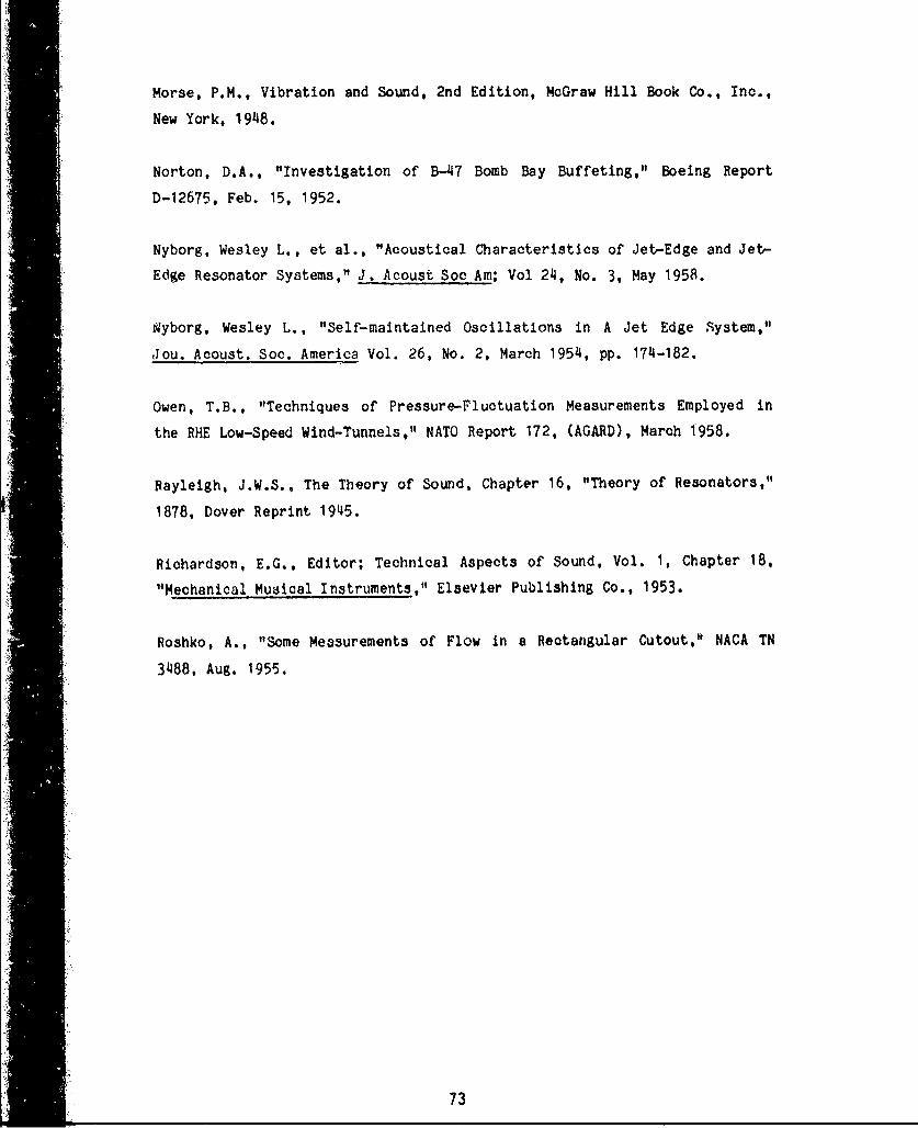
Morse, P.M., Vibration and Sound, 2nd Edition, McGraw Hill Book Co., Inc.,
New York, 1948.
Norton, D.A., "Investigation of B-47 Bomb Bay Buffeting," Boeing Report
D-12675, Feb. 15, 1952.
Nyborg, Wesley L., et al., "Acoustical Characteristics of Jet-Edge and Jet-
Edge Resonator Systems," J. Acoust Soc Am; Vol 24, No. 3, May 1958.
gyborg, Wesley L., "Self-maintained Oscillations in A Jet Edge System,"
Jou. Acoust. Soc. America Vol. 26, No. 2, March 1954, pp. 174-182.
Owen, T.B., "Techniques of Pressure-Fluctuation Measurements Employed in
the RHE Low-Speed Wind-Tunnels," NATO Report 172, (AGARD), March 1958.
Rayleigh, J.W.S., The Theory of Sound, Chapter 16, "Theory of Resonators,"
1878, Dover Reprint 1945.
Richardson, E.G., Editor; Technical Aspects of Sound, Vol. 1, Chapter 18,
"Mechanical Musical Instruments," Elsevier Publishing Co., 1953.
Roshko, A., "Some Measurements of Flow in a Rectangular Cutout," NACA TN
3488, Aug. 1955.
73

- : T ypical high-wing low-floor transport aircraft
" -adopted to launch missiles
_.. _ __ __ -_ _ • through the sidewall.
Idealization of Missile Bay
Stream Flow
hTypical hgh-wing low-'•- ~floor transport aircraft
adapted to launch missiles".• (.W) "" ____. through the floor
"Idealization of Missile Boy
"Stream Flow -
Conventional bomber aircraft;-r ---------- fuselage bomb bay.
JIldea Idealization of Bomb Bay.
Stream Flow
Figure 1. Cavity Arrangements in Cruise Missile Carrier Aircraft
and in Conventional Bombers
74

II
-- " Long Missile Bay Open DirectlyTo Parallel Stream Flow; No Neck.
L Idealization Of AboveMissile Bays For Analysis
-'Stream Flow ___..Descriptive Da t.
Circular Missile Bay Cross Section, For Which x 100, r 7.5x
Rectangular Aperture;L = 26' L = 4', L = 0x z
Aperture Downstream Edge Coirncident With Missile Bay Aft Bulkhead.
.Lon Missile Bay, Separated From ParallelFlow Stream By A Well-Defined Neck
Idealization Of Above
Missile Bays For Analysis
-..:Stream Flow,."Descriptive Data:
Rectangular Missile Bay Cross Section, For Which 1 100', 1 =e, 1 9'.x yRectangular Aperture; For Which L 26', L 6', L 6'.
x y z
Aperture Downstream Edge Coincident With Missile Bay Aft Bulkhead.
Figure 2. Long CMCA Missile Bays Selected For Analysis
75

II
_ ,.•:-'-: ::.--.i-, .. . , =:[CASE 3.]
"Short Missile Bay Open Directly ToParallel Stream Flow; No Neck
Idealization Of Above MissileBoys For Analysis
Descriptive Data: -Stream Flow-.'"
Circular Missile Boy Cross Section, Wherein I = 26', R 9'.
Rectangular Aperture, L 26', Ly z
Aperture Upstream And Downstream Edges Coincide With End Bulkheads.
Forward And Aft Missile Boys And Apertures Are Identical.
S. .. ... .... .. .. . cAsE 4:1S©*• Short Missile •Jy Seporated From Parallel
Stream Flow by A Well-Defined Neck.
Idealization Of Above MissileBoys For Analysis
Descriptive Data: Stream Flow-
Rectangular Missile Boy Cross Section, Wherein Ix 32, 1 16', z 15'
Rectangular Aperture, For Which L = 26', L 4', L 3'x y z
Aperture Centered On Missile Bay Length.
Figure 3. Short CMCA Missile Bays Selected For Analysis.
16

Long Missile Bay With Aft-K I• "End 2ening Directly To
Non-4 arallel SeparatedFlow Stream
-Stream Flow-N..
Idealization Of AboveMissile Bay For Analysis
-StreumDescriptive Data:
Circular Missile Bay Cross Section, Wherin I 165. r 8x
Circular Aperture, Wherein L = 0, r = 8'x
Aperture May Be Perpendicular Or Canted To Flow.
"Clasical Bomb Bary; Ore
GteWoll Rn ToParallel Flow Stream
Idealization OfAbove Missile BaysFor Analysis
• ;i.Stream Flow-
Descriptive Da.to-
Rectangular Missile Bay Cross Section, Wherein 26', = 13', e 13'x y
Rectangular Aperture, Wherein Lx= 26', L = 13'K y
Aperture Constitutes One Side Of Missile B&y Enclosure
Figure 4. Aft Launch And Conventional CMCA Missile BoysSelected For Analysis
77

CATEGORY I MISSILE BAYOpen directly to stream flow; no defined throat.
Variable length, width, depth,cross section, and clutter.
Stream Flow-=_____
APERTUREVariable aperture length and width.Variable aperture location fore/aft,Variable end bulkhead proximity to aperture.
Separated from parallel flow strea~m by a clearly_ _ defined throat
•,.~~~~ ...... = tqm. ........ • • 7.•...,,-/---
-Streamn Flow- ____
LAUNCH BAY OR THROAT '/- APERTUREVariable location along missile boy. Variable length and width.Variable length, width, depth, Variable location along ftselage.cross section, and clutter.Variable end bulkhead p•oximity to aperture.
Figure 5. Generic Representation of CMCA Missile Boys
78

-Stream Flow
r- CATEGORY 3 MISSILE BAYOpen directly to non parallel flow stream; no defined throat
APERTURE:Variable aperture location fore/aft.Variable length, width, and cross section.Variable wall thickness.Variable air -low angle of incidencerelative to plane of opening.
CATEGORY 4 MISSILE BAYConventional rectangular bomb boy.
Variable length, width, depth,cross section, end clutter.
~~ Stream Flow
ýAPERTURELength orA width some as missile boy.
Figure 6. Generic Representation of CMCA Missile Boys
79

PLENUM '4
FLOW FENCEY
Figre . AP ERTUREFoilt

Figure 8. Aperture Viewed From' Bock Side of Flow Plane,
and Test Model in Position.

FREE STREAM VELOCITY VARIATION OVER APERTURE
.88
. 7_ .87
.86I , I ,
UPSTIREA .•' ENTER DOWNSTR.EAM
E'DCi EDGE
POSITION ALONG APERTURE
1.0
Ln8 BOUNDARY LAYER SURVEY
6 -M =.73
0',,LU
160~
0 .5 1.0
FRACTION OF FREE STREAM VELOCITY
Figure 9. Test Facility Flow Conditions At The Aperture
82

Ij Figure 10. Representative Category I and Category 2 Models.

IR
Figure 11. Category 3 Model With Two Aperture Configurations, and InstollationIn Flow Stream.
If~

1 4,
Figure 12. Category 4i Mod~els with Spacers to Vary L/'D.

150 .16M 150
150 150 11 08m
110 o.63 0 2000 HRZ20,000
150- .56M10M
dB - ~150
0 2000 5000 ' 22-j
HERTZ 150
ALL SPECTRA ARE IN DECIBELS WITH 97M10 dB PER DIVISION. FREQUENCY 150.,-MSCALE IS LINEAR AND VARIES AS A~IlNOTED. STREAM FLOW MACHNUMBER IS NOTED ON EACH .95MSPECTRUM. ANALYSIS BW IS FREQ. 150 - ,.SCALE UPPER LIMIT + 400.
j dB
0 2000 10,000
HERTZ
Figure 13. Response Spectra Measured at Various Flow Velocities.Rectangular Cavity, 18" X 5.75" X 5.75" with 0.5"Neck, Aperture Located at Downstream End.
86
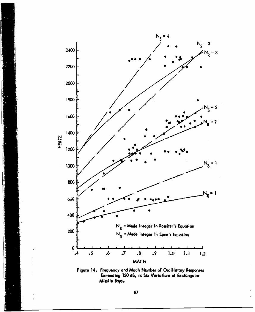
NS=4SNS 3
2400 N=3
2200 " 0
2000
1800
Ns 2
1600 oo
0 0°1400
w0
%200::1200 00 0 • e*4°e
SNI
800
0 0i::i 'i i m:400 /
NR = Mode Integer In Roulter's Equation200 N = Mode Integer In Spee's Equotim
.4 .5 .6 .7 .8 .9 1.0 1.1 1.2
MACH
Figure 14. Frequency and Mach Nunber of Oscillatary ResponsesExceeding 150 dB, Jr. Six Variations of Rectangular
Missile Bays.
87

o MODERATE RESPONSE ( LESS THAN 147 dB)
*STRONG RESPONSE (OVER 148 dB)
NI NX=6, NZ2400 NZ= U 0 00 =
2200 N = 6 0 0
20000
1600 0
N 5`4 4 NRj00
0 00
16000 0 Z/N 1zNX 1 X N N1 R /
014000
600
X 00 0 1
N 0l
2000
1N0 Mod Intge In RsIe'Euio
0 ~ ~ ~~ 0
.4 .5 6 .7 . .9 1001. 1.IN 2:ACH
Fiue1.PeunyadMc ube fRsossi etnua600X57~ *71 isl a wt "AetreAd12 ek
NR8

150 2nd
140 4th
130 6th
120
110 .38M
140 2nd 5t t1st 4th
120
110
dB ACOUSTIC FORE-AFT
RESONANCE MODES
1202
110130 .12M•
HELMHOLTZ
MODE 2ndi
120 4th
110
0 500 1000
HERTZ
Figure 16. Helmiotz Response in o Large Missile Boy Equipped with a Neck.
89

4.0
. 3.0
0
U.
La.
U
S 2.00U
FROM THE WORK OF L.F. EAST*(REFERENCE 19)
1.00 1 2 3 4 5 6 7
LENGTH TO DEPTH RATIO, L /I
Figure 17. Covity Depth Con'ection fe -'NpthwiseAcoustic Models in Conventional Bomb Boys.
90

3.8
"x"3.4 ------ -----------
FLOW
3.0
0-
> 2.6
U.
ib 2.2
' 5)4
1.4
0 1 2 3 4 5 6 7
LXLENGTH TO DEPTH RATIO
f*gum 18. Cavity Depth Correction for Depthwise Acoustic
Modes in Cotegory 4 Missile Boys.
91

EXPERIMENTALLY
N 4 0.9Mx
8dB ,5 6 10 12:/• 9
ft p ,
0 1000 2000HERTZ
ANALYTICALLY
N C00 (1 + .2M 2) 1/2
21.f x.
COMPARISON
MODE FREQUENCY HERTZORDER"x EXPERIMENTAL CALCULATED
"1 154 1502 293 2993 440 4494 597 5985 747 7486 887 8987 1049 10478 1202 11979 1352 134610 1492 149611 1646 164612 1800 1795
Figure 19. Fore-Art Acoustic Resonance Frequencies
Calculated and Measured in a 44" Missile Bay.
92

150 77M 15
.71M.' AMO
150 150
150, 7150
- I I " . 62M . . . . .-
150 LAIII&IM&150-
150 1000 5000 0 1000 5000
HERTZ HERTZ
ii: NOTE: ANALYSIS 8W 1 2.5 XERTZ!. ALL SPECTRA ARE IN DECIBELS, 10dB PER DIVISION. THE FREQUENCY SCALE IS LINEAR,
10 TO5000 HERTZ IN ALLCASES. FLOWMACH NUMBER IS NOTED ON EACH SPECTRUM.
Figure 20. CMCA Case 1 Response Test SpeclwuCylinc~rikal/• ';i•Missile Bay 23.2• X 5.4" i).
93
*I'• •mm qm ~ qliilmnmnmm qm~m mmqmdi lw


150 150 150 K ! t
.65M .95M .8150 150 1••150 .. •,••
150 .61M
150 150
150 -- 15 51m 150 1.H0 0
150 J1.~ 03IM150 ~.AAAL150
t 150 AA7 N I 0 1. VOm150 j150 J~
FRE EN0L IS L0 1000 H.5000
150nria M.4lM HEy6RTZ.4D
1150
150 95150 i
0 1000 HERTZ 500 0 1000 HERTZ 5000
NOTE: ANALYSIS BANDWIDIH IS 12.5 HERTZALL SPECTRA ARE IN DEiCIBELS,, 10 dIB PER DIVIS'ON. THEFREQUENCY SCALE IS LINEAR, 0 TO 5000 HERTZ I i ALLCASES. FLOW MACH NUM8BER IS N~OrED ON %rACH SPECTRUM.
Figure 22. CMACA Case 3 Response Test Spectrr.Cylindrical Missile Bay 6"1 X 5.40 D.

150-%Wvv " *77hA 150 1 9
150 475M .ol150
150 .31.07
1150
150
15050.
15015
IIS
0 HERTZ 0 1000sw
NOTE: ANALYSIS BANDWIDTH IS 12.5 HERTZHRTALL SPECTRA ARE IN DECIBELS, 10 dB PER DIVISION. THEFREQUENCY SCALE IS LINEAR, 0 TO 5000 HERTZ IN ALL
F CASES. FLOW MACH NUMBER IS NOTED ON EACH SPECTRUM.Figure 23. CMCA Case 4 Response Test Spectra.
Rectangular Missile Bay 6"1 X 5.750 X 5.75" .96

150 .77 15.06M
150172 150
150 .7 5
15.0
150 .59 15
150 150 .9
100 1000 HERTZ 50
46M NOTE.ALL SPECTRA ARE IN DECIBELS, 10 dB PER
L DIVISION, THE FREQUENCY SCALE IS[ ~LINEAR, 0 TO 500 HERTZ IN ALL CASES.150 FLOW MACH NUMBER IS NOTED ON EACH
___ SPECTRUIM. BW 12.5 HERTZd8B
0 l~~ HERTZ 50
Figure 24. CMCA Case 5 Response Test Spectra.CylInI dricalI Missi le Bay, 70 X .850 D. Aft Launch.
97

1.* 07M1150
15015
150 .7M 1150
1500
15015
7150
150 .4150
1550
150 _5M10 1000 HMT
ddB
0 1000 5000
HERTZ
NOTEXI PECTRA ARE IN DECIBELS, 10 dB PKR DIVISION. THE FREQU)ENCY SCALE ISV NEAR, 0 TO 5000 HERTZ IN ALL CASES. FLOW MACH NUMBER IS NOTED ONEACH SPECTRUMA. ANALYSIS BANDWIDTH IS 12.5 HERTZ
Figure 25. CMCA Case 6 Respons Test Spectra.Conventional Bomb Bay, 6" Aperture,. 3" Depth.
98

2.8
2.6
2.20.
(0 .0
AN 5 1
Rgur 26ConptedShec Laer ad Aou~tC Mdes
CyN nrIa Mis.l Bo,2" ."),W
6' AprtuAe
NO.9
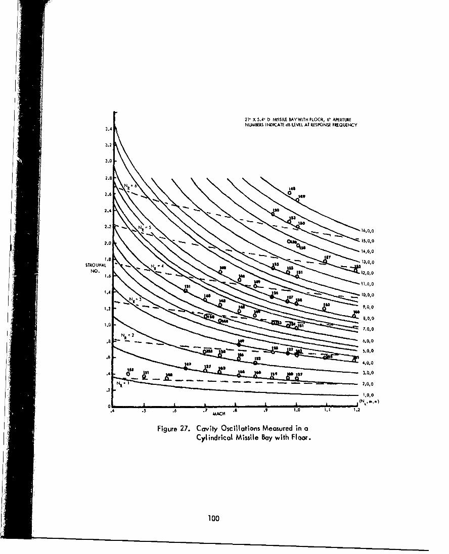
21" X 5.4" D hM$SU.E BAY WITH rLOOR, 6' APERTURENUMBERS INDICATE dB LEVEL AT RESPONSE FREQUENCY
3.4
3.2
3.0
NO.8
2.4 0,0
2.2 5 o 16,0,0o
65,0,0
14,0,0
.I a,.0,0
NO. 41 1, 0, 0
11,0,0
t.4I
Fiur 27 411yOs~lt~sMesrdiC1.nrio M9sieB01it0lor
100,

21' X 5.4 D) MISSILE SAY WITH4OUT FLOOR, 6' APER7121NW*MES INDICATE d$ LEVEL AT RESPONSE FUGQL.IECY.
~3.0 0
2.68
N 2.4s
1.01
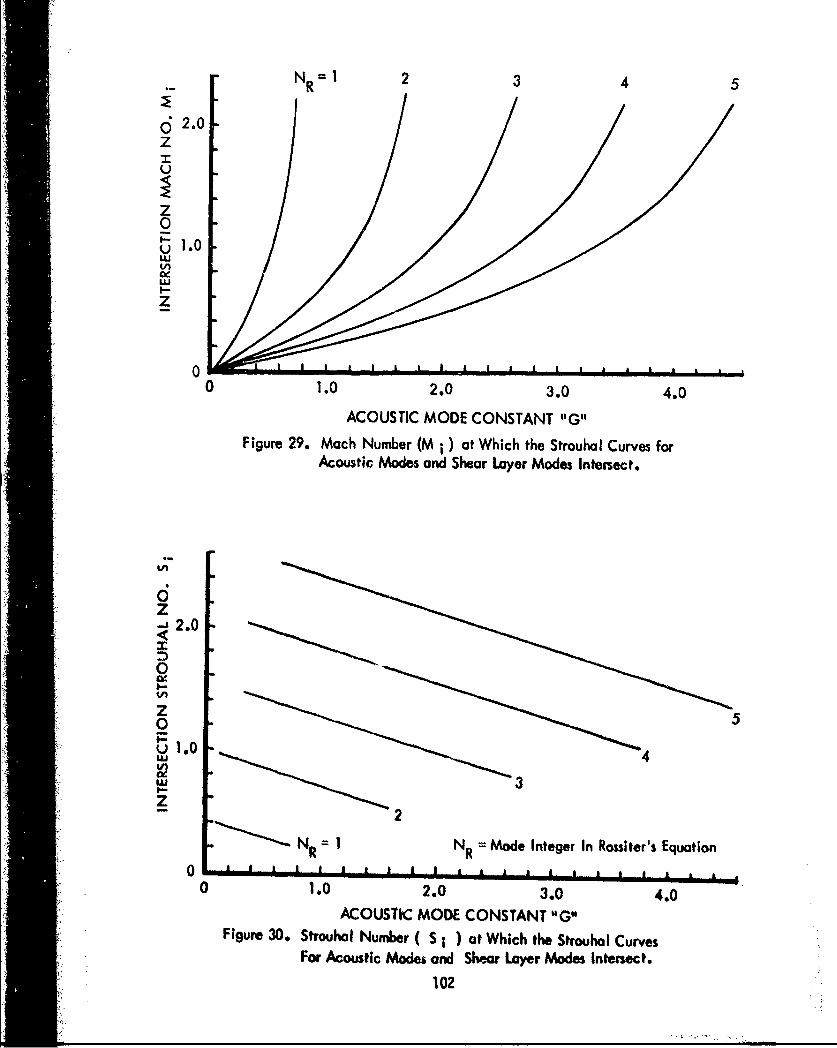
N R 2 3 4 5
62.0z
z0
S1.0
LU
00 1.0 2.0 3.0 4.0
ACOUSTIC MODE CONSTANT "~GilF igure 29. Mach Number (M i ) at Which the Strouhal Curves for
Acoustic Modes and Shear Layer Modes Intersect.
z-J2.0
0
z 50U 1.0U)
2
R 1 R Mode Integer In Rossiter's Equation0 11111iIII i ip*f
0 1.0 2.0 3.0 4.0ACOUSTIC MODE CONSTANT IIG"
Figure 30. Stroukol Number S; at Which the Strouhal CurvesFor Acoustic Mode" and Shear Layer Modes Intersect.
102

PSI
TIME
DISTORTION, NEAR NODE PLANE
PSI
TIME
Figure 31. Example of Oscillatory Sound Pressure Wave Distortion.
103

150 150
150 1503
0 2o00 1 0 20020000
150 II . .6 1 150 J 1.M
150
I II it IL
0 2000 M 0 2m0 10000
1,50 L
"50O0 Ao I
0 "00 m~1z 50 0 "20000NOTE: ANALYSIS BW IS FREQUENCY SCALE UPPER LIMIT 4 400.ALL SPtCTRA ARE IN DECISELS, 10 dll PER DIVISION. FREQUENCY SCALE IS LINEARAND VARIES AS NOTED. FLOW MACH NUMBER IS NOTED ON EACH SPECTRUM.
Figure 32. Response Spectro Mecsumred in a Cyllndrical Miuile Bay,21 x 5.4" D, No Flooe, 6" Aperture at Downstreo End.
104

i50
0 640 HERTZ
120
0 1 2 3 4 5 6 7 8 9 10 11 12 13 14 15 16 17 18 19 20 21STATION
150
100 0 320 HERTZ120 ,.I~COSNt)
0 1 2 4 5 6 7 8 9 10 11 12 13 4 15 16 17 8 1 2021STATION
Figure 33. SPI Spatial Variation Fore-Aft in 21 "x5.4" D. CylindricalMissile Say, At Mach 0.81, 320 and 640 Hertz Modes
0 0 0000
IS0dO 0
140
1275 HEMI
120
o 1 2 3 4 5 6 7 8 9 10 1 W 1' 14 1 IS t6 17 18 19 2D 21STATION
140 0 0dl0 0 0
13D 6 ~r
0 1 2 3 4 5 -6 7 4 9 10 It 12 13 I4 IS 16 17 13 It 20 21STATION
Figure 34. SPI. Spatial Votlatior Fore-Aft In 21 x S. 54" D. Cyl i'tdricalMissile Say, At Mach 0.31, W0 And 1275 Hertz Modes
105

160
150000 0
1400
dB
120
0 1 2 3 4 5 6 7 9 10 11 12 13 14 15 16 17 18 19 20 21
STATION
sP6 ICOS (Nir•) I MEASURED160 x
0 0 0150
dB 10'l125
0 1 2 3 4 5 6 7 8 9 10 11 12 13 14 15 16 17 18 19 20 21
STATION
Figure 35. SPL Spatial Variation Fore-Aft !n 21 " x 5,.4" D. CylindricalMissile Bay, At Mach 0.81, 2550 -And 3825 Hertz Modes
106

2~L/D I
2.6 ~Solid Symbols Indicate Intense Response
o . -
21.4
20
1.80
z .6
2,0Z
1070

L/D= 22.8
Solid Symbols Indicate Intense Response2.6 N "6 Open Symbols Indicate Moderate Response
2.N /p, - --........
2.02.0
0 1.8z
. 1.4 N "- '0
1.0
.6
R--.2
0 * *w
.4 .5 .6 .7 .8 .9 1.0 1.1 1.2
MACH
Figure 37. Roste' Measured Oscillotory Response (Frmn Reference 2)Correlaoted With Predicted Acoustic Modes For L/D 2 Covity, L~ 8"
108

2.8 N =6 L/D 8
2.6 open Symbols Indicate Moderate R.sPonse
2.4
2.2 NR R
2.0--
1.8 NR 4
1.6 -
Z R20
0 1.0 0
.2
.4 .5 .6 .7 .8 9 1.0 1.1 1.2
MACH
Figure 38. Roslter~s Measured Oscillatory Respons (From Reference 2)Corelaed ithPreicted Acoustic Modes for I)8 Cavity.I. L B.
109

COMPOSITE PLOT OF NORMALIZED MAXIMUM OSCILLATORYSOUND PRESSURE LEVELS FROM TEN VARIATIONS OF CYLINDRICALMISSILE BAYS.
-10
-20
00 3
-40
.4 .5 .6 .7 .8 .9 1.0 1.1 1.2
MACH
Figure 39. Development of Empirical Curve For Sound Pressure Level Predictions.
-10
WITH FLOORL
MI <~ .56, 20LOG P/q 22.8BM w3 .3 x+ 1~6 L
Mi >.69,,20OLOG P/q + -14.5 M -6.6+ 16-.
.564ML < .69, USE EQUATION PREDICTING LARGEST NEGATIVE VALUE.
WITHOUT FLOORL
OMIT THE "NECK"' ERM, (16 T IN ABOVE EQUATIONS.
.4 .5 .6 .7 .8 .9 1.0 1.1 1.2MACH
Figure 40. Normalized Maximum Oscillatory SPL in Cylindrical Missile Boys.
110

-10
~-203a-
004
-40 L xL
FOR L 31 20 LOG P/q = 8.7 M -2 ~8.5LX LX
.4 .5 .6 .7 .8 .9 1.0 1.1 1.2
MACH
Figure 41. Normalized Maximum Oscillatory SPL in Rectangular Missile Boys.
-10
2r, LOG P/q(dB)
-30- 20 LOG P/q -35.9 M'+ 84.4 M L5
.4 .5 .6 .7 .8 .9 110 1.1 1.2MACH
Figure 42. Normalized Maximum Oscillatory SPL In Conventional Bomb Bays
ciyi

AdB = 20 LOG P/q@M-20 LOG P/q@Mi, or= SPL@M-SPL@M.
0 "
-2
-4
AdB-6
-8
-10I I I I I I I S I * i i a I A £
M M +M M. M. +Mt Mt
2 2MACH NUMBER
Figure 43. Oscillatory SPL Variation With MachNumber Between Onset and Termination
112
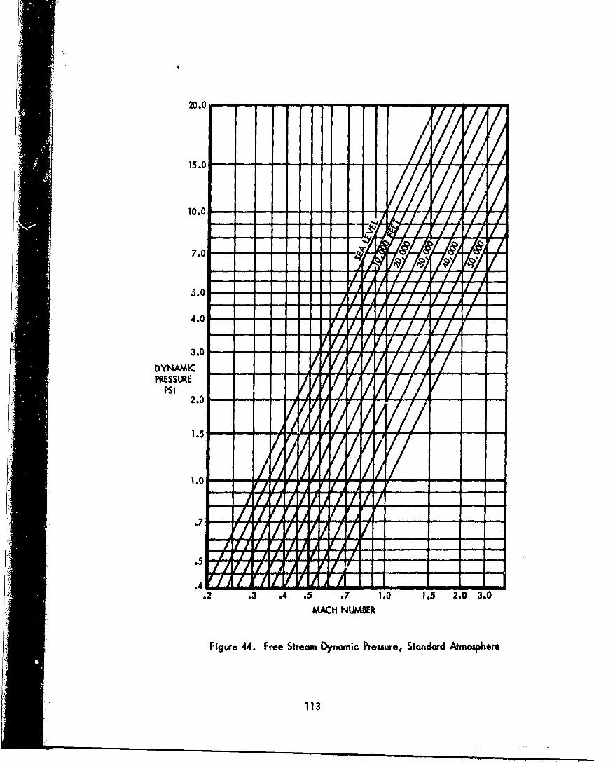
15.0A
10.0. -a
7.0-
%. -
4.0-
3.0 1-
DYNAMICPRSSIAtE
PSI 2 .
.7
.2 .3 .4 .5 .7 1.0 1.5 2.0 3.0MACH NUMABER
Figure 44. Free Stream Dynamic Pressure, Standard Atmospere
113
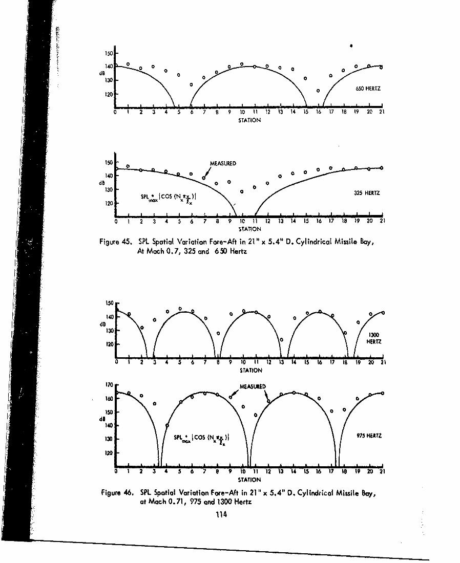
T,
150
140 014 0 0 0 0 o0 0 0 0 00
3 0 0 0 00B 0 60 0ET
02 00 0 3250HERTZ
0 1 2 3 4 5 6 7 8 9 C 101 12 13 14 15 16 17 18 19 20 21
STATION
AtO Mah0E,35 A SUR0 ErD
9 0 0 0
140 0 o
0130 0r 2 ET
1200 ET
0 1 2 3 4 5 6 7 8 9 10 11 12 13 14 15 16 17 IS 19 20 21STATION
150
140
0 0120
0 1 2 3 4 5 6 7 8 9 10 11 12 13 14 15 16 17 IB 19 20 21STATION
1414

1500
140 0 0 0 0 0 00dB 0 0000
130 0 0 0
120 01775 HERTZ
0 1 2 3 4 5 6 7 8 9 10 11 12 13 14 15 16 17 18 19 20 21STATION
150
140 00 0 0 0 0 0 000 0 0 00 0 0dB 000
130 0 0 0
1201600 HERTZ
o~~ 1It 5 6 7 8 01 12 13 14 15 16 17 18 19 20 21STATION
Figure 47. SPL Variation Measured Fore-Aft in 21" x 5.4' D. Cylindrical Missile Bay,at Mach0. 71, 1600and 1775 Hertz
150
0 0 0 0 0140 a0 0 000 0 0 0
(60 00 000
130
120 2250 HERTZ
0 10 6 7 8 9 t 11 12 13 14 15 16 17 18 1260 121STATION
06 0 0 0 0 00
150 0 0 0 0000000 0 0
0 0 014000
da
1950 HERTZ120
o 1 2 3 4 5 6 7 8 9 10 I'l 12 13 14 15 16 17 18 19 20 21STATION
Figure 48. SPI Variation Measured Fore-Aft in 21" x 5.4" D~. Cylindrical Missile Bay,at Mach 0. 71, 1950 and 2250 Hertz
115

170
00
dB CURVE 1275 HERTZ1 BROADBAND
PR\130 - NOISE FLOOR I
THEORETICAL IMODE AT .81M.120 - I t--COSINE CURVE--,
0 1 2 3 4 5 6 7 8 9 10 11 12 13 14 15 16 17 I 19 20 21
170 STATION
160 0
1500do0 I •"EMPIRICAL CURVE % H
130 BROADBANDPRNIA
10TH4EORETICALIIMOEA.7M
0 1 2 3 4 5 6 7 8 9 10 11 12 13 14 15 16 17 18 19 20 21
STATION
Figure 49. Fore-Aft SPL Variation Given by Equation 34 Which Accounts for BroodbandNoise Level, 21" Cylindrical Missile Bay
1
116

-30 .4M
-351/3 OCTAVE.8
-40
20 LOG P/qI 2
-45
.2 .4 .7 1 2 4 7 tof LX
Figure 50. Broadband SPL at Downstream Wall Nekar Aperture
0
-5
AdB
&dBmt dB POINT z-d8 AP~ERTURE
0 1.0zAx
Figure 51. Depthwise Variation of Broadband SPL on Do'wnstreoni End Wall
117

4k
MAXIMUM CLUTTER IN SHORT MISSLE BAY -VALL REMOVED)
170-i6 CLUTTERED16o "-
140
170CLEAN160-
150 ,dB
140
" 2 t
0 1000 2000 3000 4000 M00
HERTZ
Figure 52. Effect of Clutter on Frequency and Level of Maximum Csciflotion.
Il8

MAXIMUM CLUTTER AND BLOCKAGE IN CONVENTIONAL BOMB BAY
17017ot CLUTTERED
160++150 + 4
170 •. .16o ± "CLEAN160~~
dB150-
140o+
0 1000 2000 3000 4000 5000
HERTZ
Figure 53. Effect of Clutter and Partial Olockage on Frequeiwcy andLevel of Maximum Oscillotion.
119

2.8 -N= 6 NR = Mode Integer In Rossiter's Equation
2.4 N
2.0
0
58.1.2
N R =2
.8
.4 .5 .6 .7 .8 .9 1.0 1.1 1.2
MACH NUMBER
Figure 54. Sheam Layer Oscillation Modes.
120
~..... .... 66

2.4
2.0
STROUHAL
8,0
1.21

2.4
2.0
1.6
STROUHALNO.
.8
MACH
Figure 56. Speed Ranges Of Probable Modes Of Oscillation Predicted for CMCA Case 2
122

160 1. z -s6
150 15.6 Hz
dB 5
140
.4 .5 .6 J1 .8 .9 1.0 1.1 1.2MACH
Figure 57. CMCA Case 2 Response Frequency and Maximum SPLPredicted for 25,000 Feet
160
150
140SPECTRUM
LEVELdBr
130
120
HERTZ
Figure 58. CMCA Coo 2 Maximum Oscillatory Sound PressureSpectrum Predicted For ASM, 25,000 Feet
123

160
150
140
130rBROAýDBAND
120 - -
0 J1 .2 .3 .4 .5 .6 .7 .8 .9 1.0
160
150
(2)(4,0)140 21.6 Hz
dB130
BROAD BAND120
o .1 .2 .3 .4 .5 .6 .7 .8 .9 1.0X/1 x
160
150OVRLdB
140
0.1.2.45 .607 .8.9 1.0
K/x
Figure 59. CMCA Case 2 PN.dicted Fore-Aft Variation In SPL On WallOpposite Aperture,. for ABM at 25,000 Feet
124

CMCA Oscillation Mach No. Of Oscillation MaximumCa.. Mode On- Inter- Ternin- Frequency SPL
# (Nx, N) Set section ation Hertz dB
(I)(1,0) - .37 .75 5.2 153(1)(2,0) .59 1.02 - 11.2 161(2)(3,0) .43 .52 .61 15.6 157(2)(4,0) .65 .78 .95 21.5 160
I (2)(5,0) .94 1.17 - 28.7 162
2 (1)(1,0) - .37 .75 5.2 146(1)(2,0) .59 1.02 - 11.2 158(2)(3,0) .43 .52 .61 15.6 150(2)(4,0) .65 .78 .95 21.5 155(2)(5,0) .94 1.17 - 28.6 159
3 (2)(1,0) .61 .74 .88 20.6 160(3)(1,0) .36 .40 .43 19.8 154(3)(0,1) .75 .83 .91 35.2 161(3)(1,11) .96 1.08 42.7 161
4 (2)(1,0) .46 .55 .65 16.4 143(3)(2,0) .70 .78 .85 33.6 153(3)(0,1) .78 .86 .95 36.3 156
5 Nore - - - None -
6 (1)(,01) .68 1.2 12.6 178(2)(1,0) .61 .74 .88 20.6 163(2)(1,1) .76 .93 1.13 24.3 172(3)(0,2) .76 .84 .92 35.5 168
Figure 60. Predicted CMCA Missile Bay Oscillation Within the Speed Range of.4M to 1.2M, at 2000 Feet
125

CMCA Oscillation Launch Oscillation Maximum BroadbaoACase Mode Altitude Frequency SPL Spectrum Level
(NR)(Nx,NF) Feet Hertz dB dB.
1 (1)(2,0) 25Mo0 10.8 159 123
S37000 10.3 154 118
(2)(4,0) 2500 21.6 160 122
37000 20.6 155 117
2 (1)(2,0) 25000 10.8 156 121
37000 10.3 149 118
(2)(4o0) 200 21.6 155 122
37000 20.6 15C 117
3 (2)(1,0) 25000 20.8 158 123
37000 19.8 153 118
4 (3)(2,0) 25000 33.7 151 120
37000 33.1 146 115
5 None - -
6 (1)(0,1) 25000 11.8 162 125
37000 11.2 157 120
(2)(1,1) 25000 2•.9 162 122
37000 221 157 117
Figure 61. Predicted Ct,,ACA Missile Bay Ocillation At Mach 0.8, AltitudesOf 25000 And 37000 Feet
126
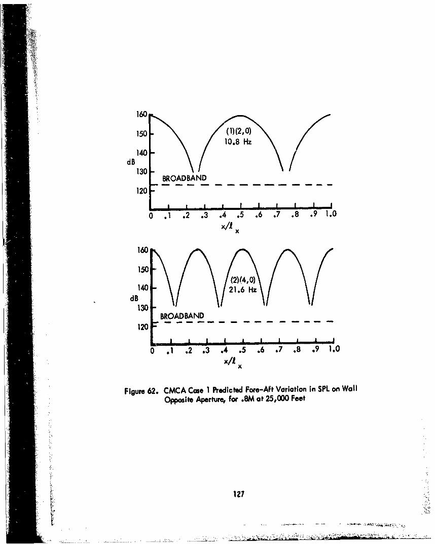
160
150 ()20
140-
dB130 [ ý / 00BROADBAND
120
0 .1 .2 .3 .4 .5 .6 .7 .8 .9 1.0
160
150((2) (4,0)
140 21.6 H
d130 2 z
[BROADBAND120
I I I - L A 3 a a
0 . 2 .3 .4 .5 .6 J7 .8 .9 1.0
Figure 62. CMCA Case 1 Predlicted Fore-Aft Variation in SPL on WallOpposite Aperture for .8M at 25,000 Feet
127

160
1S0
140dB208H
130
120
0 .1 .2 .3 .4 .5 .6 .7 .8 .9 1.0X/
Figure 63. CMCA Case 3 Predicted Fore-Aft Variation in SPLOn Wall Opposite Aperture, For ,8M at 25,000 Feet
160
150
140337HdB
130
120 BROADBAND. 120 - "- - --- -- - ---
S. 1 ~ ~ ~ I 1._ i 1 I .I .. ... 1 _ I
0 ,1 .2 .3 .4 .5 .6 .7 .8 .9 1.0x/1 x
Figure 64. CMCA Case 4 Predicted Fore-Aft Variation In SPLOn Wall Opposite Aperture, For .JM at 25,000 Feet
128
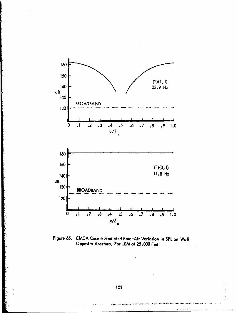
160
150
140 23.? HzdB
BROADBAND
120-
I i i I - I I I I a
0 . .2 .3 .4 .5 .6 .7 .8 .9 1.0x/i
X/
160
15()(o, 1)
140 11.8 Hz
dB130 BROADBAND
120
I I .. . I .... 1_ I. .... iI. __. 1 _
0 .9 02 .3 .4 .5 .6 .7 .8 .9 1.0
x/Ix
Figure 65. CMCA Case 6 Predicted Fore-Aft Variation in SPL on WallOpposite Aperture, For .8M at 25,000 Feet
129

170
160
150(2) (1, 1)• 150
SdB 23.9 Hz• ~140 -
" ~~~~~~~BROADBAND m= m= == ,i ie== I•
130 -•
120
S I I -A I I C I
1.0 .9 .8 .7 .6 95 .4 .3 .2 ,I 0
170
160
150 dB I 1.8 HzdB
140 BROADBAND -- ....woo
130
120
1.0 .9 .8 .7 .6 .5 .4 .3 ,2 ,I 0
z/
Figure 66. CMCA Case 5 Predicted Depthwise Variation In SPL on Dwnstream Wall,For .AM, gt 25000 Feet.
130

TRSI
MA,
livonto ofSey oe

1.0151.1M
A -
150 150, 1.21M
150, 150 .89m I
150. 150
15,0 .77t ,
ISO --- 0
ISO .43MIS
0 HERTZ 0 1000 HERTZNOQ ALLEVIATION WITH ALLEVIATION
NOTE,
ALL SPECTRA ARE 10 d8 PER DIVSION, LINEAR -REQIJENCY SCALE0 TO M00 HERTZ. STEAM FLOW MACH NUMR IS NORD ONEACH SFECULIM.
Figure 68. CMCA Case 1 Response Spectra With andWithout Spoi ter/Ronp Al eviotion Devices.
132
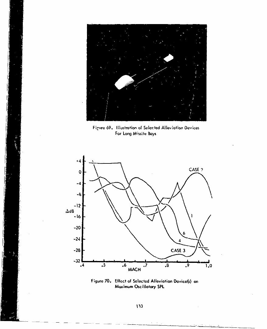
Fit~re 69. Illustration of Selected Alleviation DevicesFor Long Missile Boys
+4
CASE ?
s -43
-20-16 -
-24
-241
-28 -CASE 3
-32
.4 .5 .6 .7 .8 .9 1.0MACH
Figure 70. Effect of Selected Alleviation DWvice(s) onMaximum Oscillatory SPL
.,1

CMCA Launch Unsuppressed SuppresedCase Altitude Max. SPL Max. SPL
Feet dB dB
1 25000 160 149
37000 155 144
2 25000 156 146
37000 150 141
3 250U0 158 128
37000 153 123
4 25000 151 130
37000 146 125
5 No Oscillation
6 25000 162 147
37000 157 142
Figure 71. Predicted Maximum Levels Of CMCA Missill? BayOscillation With And Without Alleviation; LaunchAt Mach 0.8; 25000 And 37000 Feet Altitude
134
. S GOVEHNMEL NY'INIING OFFICE Mt'g-11l 2i
A ........... ....... .. ........................S.................. •" ... ..................,..-.............................".".."....".....".....'.."'-'" ....


