
I>I. _ iiREPORT NO. AFO-507-78-2
AIRBORNE RADAR APPROACH00 FAA/NASA GULF OF MEXICO
HELICOPTER FLIGHT TEST PROGRAM
!SrTES "JUN13 1980 LI) ]JANUARY 1980
Availability is unlimited. Document may be released tu the Clearinghousefor Scientific and Technical Information, Springfield, Virginia 22151 for saleto the public.
kw DEPARTMENT OF TRANSPORTATION.J FEDERAL AVIATION ADMINISTRATION
OFFICE OF FLIGHT OPERATIONSWASHINGTON, D.. 2Q,9 1 .,.' -" 6 13059
I.I
The contents of this report reflect the findings of the OperationsResearch Staff, Flight Standards National Field Office, Office of FlightOperations, which is responsible for the facts and the accuracy of thedata presented herein. The contents do not necessarily reflect theofficial views or policy of the Department of Transportation. Thisreport does not constitute a standard, specification, or regulation.
"]
30 _____,____.___ c:1

TECHNICAL REPORT STANDARD TITLE PAGE
1. Report No. 2. Government Accession No. 3. Recipiert's Catalog No.
,tF0-507-78-2 A y- ,'0 "Lg -
Ai dborne Radar Approachp 1FM/NASA Gulf of Mexico , , -.....H li co p e F1 15h e t P og a . Perform ing Organization CodaH opter Flight TestProgrm,AFO-507D d8. erforing Organization Report No.onal P. PateA .... -.ames H./Yates PhD
9. Performing Organization Name and Address U .
Operations Research Staff, AFO-507FSNFO, FAA P. 0. Box 25082 1. Contractor 0,No.Oklahoma City, Oklahoma 73125 R "o .'/4ro C
• T 3. Type of Report~div 5eriod Covered
12. Sponsoring Agency Name and Addrs' FnaOffice of Flight Operations, DOT Final part800 Independence Ave. __.
Washington, D.C. 20591 14. Spnsoring Agency Code
15. Supplementary Notes
16Abstract
A joint FAA/NASA helicopter flight test was conducted in the Gulf of Mexico to( investigate the airborne weather and mapping radar as an approach system for-offshore drilling platforms. Approximately 120 Airborne Radar Approaches (ARA)were flown in a Bell 212 by 15 operational pilots. The objectives of the testwere to (1) develop ARA procedures, (2) determine weather minimums, (3) determinepilot acceptability, (4) determine obstacle clearance and airspace requirements.
A Aircraft position data was analyzed at discrete points along the intermediate,final, and missed approach. The radar system error and radar flight technicalerror were determined in both range and azimuth, and the capability of the radaras an obstacle avoidance system was evaluated.
17. K*y Words 18. Dletrlhutlen Statement
Airborne Radar ApproachARA, Helicopter IFROffshore Helicopter Operations Distribution Unlimited
( Security Clessif. (of this report) 20. Security Clesslf. (of this page) 21. No. of Pages 22. Price
Unclassified Uncl assi fied 144
Form DOT F 17007 i-m) iii
A 1 17 6
- - ___ 4

-1
TABLE OF CONTENTS
Page
Introduction 1Test Description 1Approach Description 5
Initial Approach 5Final and Missed Approach 8
Description of Analysis 8Analysis 13
Approach Azimuth Accuracy 13Range Accuracy 59Missed Approach Dispersion 75Operational Difficulties 90
Summary of Conclusions 95Approach Tracking Accuracy 95Range Accuracy 96Missed Approach 97General Conclusions 98
Recommendations 101Approach Tracking Accuracy 101
( Range Accuracy 101Missed Approach 102General Recommendations 103
Appendix A 105Collection of Data - Final Approach 105Extraction of Data - Final Approach 105Lateral Dispersion Statistics - Intended Course 106Lateral Dispersion Statistics - Average Course 108
Extraction of Data - Missed Approach 111La':eral Dispersion - Missed Approach 113Daca Collection - Range Interpretation Error 113Statistical Analysis - Range Interpretation Error 114Data Collection - Flight Technical Error 114Data Collection - Flight Technical Error 115Statistical Analysis - Flight Technical Error 115Mann-Whitney U-Test 116Kruskal-Wallis K-Sample Test 117Kolmogorov-Smirnov Two-Sample Test 118Spearman Rank Correlation Test 119
Appendix B 121The Theoretical Homing Curve 12ZBlind Flight Path 124The Missed Approach Curve 131Conclusions - Homing Curve 137Conclusions - Missed Approach Curve 141
(- - ~v

LIST OF ILLUSTRATIONS
Figure Page
i Arcing Entry 6
2 Overhead Ehtry 73 Overhead Entry 15 Offset 94 Helicopter Airborne Radar Approach Plate 115 Overhead Outbound Turn 216 Composite Approach Tracks: Straight-In 1/2 Mile MAP 267 Composite Approach Tracks: Offset 1/2 Mile MAP 278 Composite Approach Tracks: Straight-In 1/4 Mile MAP 289 -Composite Approach Tracks: Offset 1/4 Mile MAP 29
10 Approach Envelope: All Approaches Combined 3111 Approach Envelope: Straight-In 3212 Approach Envelope: Offset 3313 Approach Envelope/Average Path: All Approaches Combined 4114 Approach Envelope/Average Path: Offset Approaches 4315 Approach Envelope/Average Path: Straight-In 4416 Error Components 4617 Aircraft Radar Position CEP 7318 Composite Missed Approach Tracks: Offset 1/4 Mile MAP 7619 Composite Missed Approach Tracks: Offset 1/2 Mile MAP 7720 Composite Missed Approach Tracks: Straight-In 1/4 Mile MAP 8021 Composite Missed Approach Tracks: Straight-In 1/2 Mile MAP 8122 Missed Approach Envelope: Offset 1/2 Mile MAP 8423 Missed Approach Envelope: Straight-In 1/2 Mile MAP 8524 Missed Approach Track of Aircraft Poorly Positioned at MAP 92
A-1 Lateral Dispersion Error: Intended Path 106A-2 Lateral Dispersion Error: Average Path 109A-3 Missed Approach Partitions 112B-1 Homing Curve Diagram 122B-2 Blind Flight Path Diagram 124B-3 Blind Segment Diagram 127B-4 Intersection of Dynamic Target Path and Blind Path 129B-5 Wind Effects on Missed Approach Path 131B-6 Crosswind Diagram 1 133B-7 Crosswind Diagram 2 133B-8 Crosswind lind Segment 134B-9 Length of Blind Segment vs Degrees of Crosswind 142
60 kt Airspeed* B-10 Distance to Path Intersection with Radar Sweep vs 143
Degrees of Crosswind, 60 kt AirspeedB-11 Length of Blind Segment vs Degrees of Crosswind 144
70 kt AirspeedB-12 Distance to Path Intersection with Radar Sweep vs 145
Degrees of Crosswinds, 70 kt AirspeedB-13 Length of Blind Segment vs Degrees of Crosswind 146
i 80 kt Airspeed* B-14 Distance to the Path Intersection with Radar Sweep vs 147
( .Degrees of Crosswind, 80 kt Airspeed
fvii
V ~ :.*-7,€*t
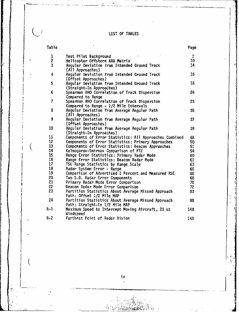
LIST OF TABLES
Table Page
1 Test Pilot Background 22 Helicopter Offshore ARA Matrix 103 Angular Devi-ation from Intended Ground Track 14
(All ApproachesG d4 Angular Deviation from Intended Ground Track 16
(Offset Approaches)Angular Deviation from Intended Ground Track 18(Straight-in Approaches)
Spearman RHO Correlation of Track Dispersion 24Compared to RangeSpearman RHO Correlation of Track Dispersion 25Compared to Range - 1/2 Mile Intervals
8 Angular Deviation 'from Average Angular Path 35(All Approaches)
9 Angular Deviation from Average Angular Path 37(Offset Approaches)
10 Angular Deviation from Average Angular Path 39(Straight-In Approaches)
11 Components of Error Statistics: All Approaches Combined 4812 Components of Error Statistics: Primary Approaches 5013 Components of Error Statistics: Beacon Approaches 5114 Kolmogorov-Smirnov Comparison of FTE 5415 Range Error Statistics: Primary Radar Mode 6016 Range Error Statistics: Beacon Radar Mode 61
17 TSE Range Statistics by Range Scale 6318 Radar System Error - Range 6519 Comparison of Advertised 1 Percent and Measured RSE 6620 Two S.D. Radar Error Components 6821 Primary Radar Mode Error Comparison 7022 Beacon Radar Mode Error Comparison 7223 Partition Statistics About Average Missed Approach 83
Path: Offset 1/2 Mile MAP24 Partition Statistics About Average Missed Approach 88
Path: Straight-In 1/2 Mile MAPB-1 Maximum Speed to Intercept Moving Aircraft, 20 kt 148
WindspeedB-2 Farthest Point of Radar Vision 149
ixI _ _ _ _ _ _

())
\./) Project Report on Airborne Radar Approach FAA/NASA
Gulf of Mexico Helicopter Flight Test Program
Project Officer Donald P. PateOperations Research AnalystOperations Research Staff
.j/~/
Approved Ted 0. McCarleyChief,r Operations Research Staff
/4.L
Released 4 11 am D. Crawford
Released Chief, Flight Standards'
National Field Office
)j
January 1980
1,1 A
ix
l*
lx

K INTRODUCTION
A joint NASA/FAA helicopter flight test program was carried out between
June 1978 and September 1978 in the Gulf of Mexico to investigate airborne
weather/mapping radar as an offshore approach system. The objectives
of the test were to:
1. Develop airborne radar approach (ARA) procedures.
2. Determine weather minimums.
3. Determine pilot acceptability.
4. Determine obstacle clearance .and airspace requirements.
The purpose of this paper is to present the analysis utilized to establish
minimums, determine obstacle clearance and airspace requirements, and
establish procedures.
TEST DESCRIPTION
The test, conducted under contract with Air Logistics, was staged from
their maintenance center in New Iberia, Louisiana. Fifteen line pilots
representing a wide range of helicopter experience (Table 1) participated
in the test as subject pilots. A standardized video tape briefing waspresented to all crews before participation in the tests. During a flight,
one crewmember served as copilot and radar controller providing course
corrections to the second pilot controlling the aircraft. Each pilot,
hooded during the tests, made eight approaches as a controller and eight
as a pilot.
I
1,

I _ _ _ _ _IAu_ _ _+
a
a I-
* ~ ~ ~ ~ ~ e @. 0C4.t lC4% InFa H. H4. 0 Nr4N4mZ4 0 m-4.44 N M
P 4 P4
In - 'o -n ,4
.U V% r4XP MM 4.
IA'4 t 44r
101 0 8100 100N9 Ar4 -4 i;n i 4-4 is0 IMM4fn%96 I:3 mI8S8 x, A~ r4
1- 8 .4 8 1.1,0. %
444
11 2Ii0
r4J tN'2 __A' N_ aJ,0r m.
A1 v4P t -

The test aircraft was a twin-turbine' Bell 212 helicopter with a two-
(N--> bladed semirigid rotor, maximum gross weight of 11,200 pounds, and
maximum airspeed of 120 knots. The radar was a Bendix RDR-1400 weather/
mapping radar, with selectable range scales, of 240, 160, 80, 40, 20, 10, 5,
2.5 nautical miles and with a stabilized 12 inch flat plane antenna having
0primary mode with selective scan angle of. ±600 or ±200. Two different
ground beacons, a Motorola model SST-181X-E and a Vegas model 367X, were used.
The approaches were flown to targets in a cluster of seven offshore
drilling platforms and oil rigs located in the Gulf of Mexico, Vermillion
Block 71 drilling area. Approaches were made to platforms in this
cluster, with the target chosen so as to provide an into the wind obstacle
free approach and missed approach.
Aircraft tracking was accomplished with a Cubic DM-43 ranging system
using three responders positioned on platforms bounding the flight test
area. The Cubic system provided a two sigma accuracy of two feet, and
including responder location uncertainty, aircraft position was established
within a two sigma accuracy of about six feet. Other onboard data collectionequipment included a 35mm camera to record the controller's panel, a 35mm
camera to record radar display, a Cubic DM-43 interrogator, an interface
to multiplex heading, airspeed, radar altitude onto magnetic tape, and an
audio cassette recorder to record onboard voice communications. Project
logs, meteorological data, chase aircraft film, pilot experience/qualifi-
cations forms, and pilot evaluations provided supplemental information to
( ' the quantitative data.
3
Ii

APPROACH DESCRIPTION
Initial Approach
The initial approach segment was accomplished with either an arcing
entry or an overhead entry. The arcing entry was designed to enter .the
final approach segment for winds within ±300 of the en rou;:e course by
flying direct to the Downwind Final Approach Point (DWFAP) while
descending from 1,000' AGL to 500' AGL. At the en route fix, the
cluster was identified, approach target chosen, DWFAP determined (for 1an into Pw0 wind approach), and the missed approach turn planned into
a clear zone free of obstacles. The approacii target was chosen on
the downwind edge typically to the right or left side of the cluster
to provide final approach and missed segments clear of obstacles. If
the approach target was not the destination, it was assumed a visual
hover taxi from the Missed Approach Point (MAP) to the destination could
be accomplished. (Figure 1)
An overhead entry was used for wind conditions requiring the cluster
be overflown to position the aircraft for an into the wind final
[ approach. Approach and missed approach planning was accomplished at
the en-route fix as in the arcing entry. The target rig was overflown
at 1,000' AGL followed by an outbound leg within ±100 of the final
approach course, descent to 500' AGL, and standard rate turn onto the
final approach course. (Figure 2)
PRECEDIiG PAG. BLAW-NOT FIiMD -.5
,-_____________
-. _ _ _ _ _

0046~I WAjiY / ITIAL FIX
(4 NM NROM
ESCEND
MAP
APPROACH TORN
it~
-~~N.U- 1

OVERHEAD ENTRY
y ,
'INITIAL FIX (RADAR IDENTIFYCLUSTER)(APPROXIMATELY 20 NM FROM TARGET)
WIND
0 OVERHEAD9o MISSED .._ TARGETAPPROACH \ 1000'TURN MISSED T
APPROACH i'POINT
0\10
-I120,OFF-
(DESCEND ,sET TTO MDA) OUTBOUND LEG
DA (DESCEND TO 500')DWFAP 4(4 NM FROM ,TARGET) "
Figure 2
7
A ';~ 4
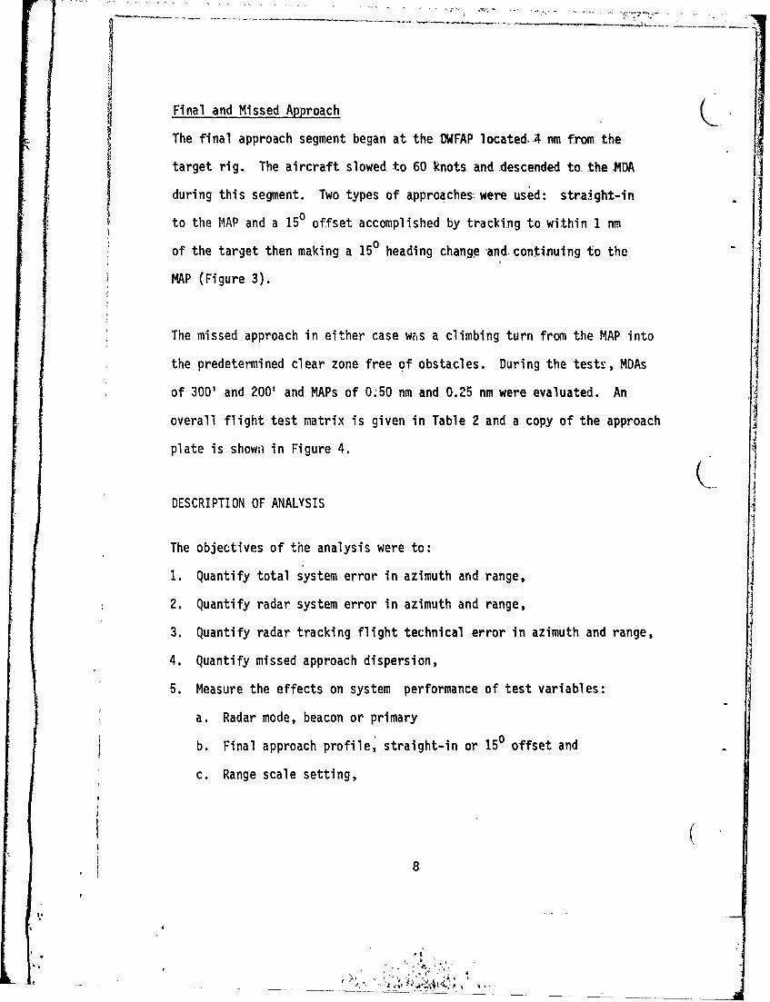
Final and Missed Approach
The final approach segment began at the DWFAP located4 nm from the
target rig. The aircraft slowed to 60 knots and descended to the tDA
during this segment. Two types of approaches- were used: straight-in
to the MAP and a 150 offset accomplished by tracking to within I nm
of the target then making a 150 heading change and, continuing to the
MAP (Figure 3).
The missed approach in either case was a climbing turn from the MAP into
the predetermined clear zone free of obstacles. During the tests, MDAs
of 300' and 200' and MAPs of 0:50 nm and 0.25 nm were evaluated. An
overall flight test matrix is given in Table 2 and a copy of the approach
plate is shown in Figure 4.
DESCRIPTION OF ANALYSIS
The objectives of the analysis were to:1. Quantify total s ystem error in azimuth and range,
2. Quantify radar system error in azimuth and range,
3. Quantify radar tracking flight technical error in azimuth and range,
4. Quantify missed approach dispersion,
5. Measure the effects on system performance of test variables:
a. Radar mode, beacon or primary
b. Final approach profile, straight-in or 150 offset and
c. Range scale setting,
(8
I.
k'
, ,£?

OVERHEAD ENTRY
15 0 OFFSET
oINITIAL FIX
WI ND
15 0OFFSET
RAP
Figure 3 p
9

WL CD CD CD CD CD CD C13 CU =D
C3 < '-3 co 4-o m- co ca co co
V)z w
CL
0- wa : 0c- 0 0 w -A c: o k
V) a- -4 tzr t4i cl l m 4 k
CL C
<C < C- ) 2:
<C WO WLm C - c - Cw~ 0w J
H e C _ _CLo) u w 4)
=- Z ZZOW CC U 4-- H 6-4 H -4 H
..j 0) z -J I WL I WL I W I wUWU c _ I-1q V /) VC) HVC)
w L-L :LL. X LL. X: U- 2:=- C) CD LL- ~ C AL CD LL tD .i _ _ = _ C_ $_ C)LL aL <C 4- - -I
w wr r - F- L - L
L4-4
Q0 0 O C c z n CwcUCY < < < cc
H 0- M u LUJ LU LU LU Lu LU LUJ
w-C C 0 0 C0 0i 0 0
LU ..J ..j .. -j --444 -4 --j 0L 0. 0L 0 CL
CC fC) Cl) V) 0l C-) CC) C)CO '-6- - -4 LU LUJ L LUJ
CDw
10

CONCENTRIC RINGSSHARKAT ~A.mi.INTERVALS
PLATFORM LOCATION TO
\. 2MISSD ME tOCIAF SCA S~t
- TIMITO~mI. 6 4.17 34 323
11 w10
I.A xI
=-4 45".g. .
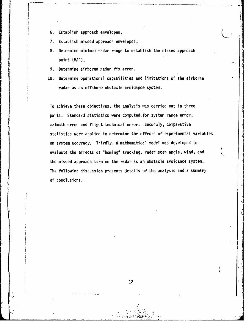
6. Establish apprbach envelopes,
7. Establish missed approach envelopes,
8. Determine minimum radar range to establish the missed approach
point (MAP),
9. Determine airborne radar fix error,
10. Determine operational capabilities and limitations of the airborne
radar as an offshore obstacle avoidance system.
To achieve these objectives, the analysis was carried out in three
parts. Standard statistics were computed. for system range error,
azimuth error and flight technical error. Secondly, comparative
statistics were applied to determine the effects of experimental variables
on system accuracy. Thirdly, a mathematical model was developed to
evaluate the effects of "homing" tracking, radar scan angle, wind, and
the missed approach turn on the radar as an obstacle avoidance system.
The following discussion presents details of the analysis and a summary
of conclusions.
(12
I.i
!,1

APPROACH AZIMUTH ACCURACY
Q_ The ability of the subject crewmembers to accurately enter and follow
the final approach path was measured from samples of the angular
deviation of the aircraft from the intended path at regular intervals
from.,the target (see Appendix A for a full explanation of the sampling
procedure). Standard statistics were computed from each sample for all
flights, offset flights, and straight-in flights.
It was found that the average angular deviation for all flights at
ranges between 5 nm and .588 nm was between +50 and +60 (Table 3).
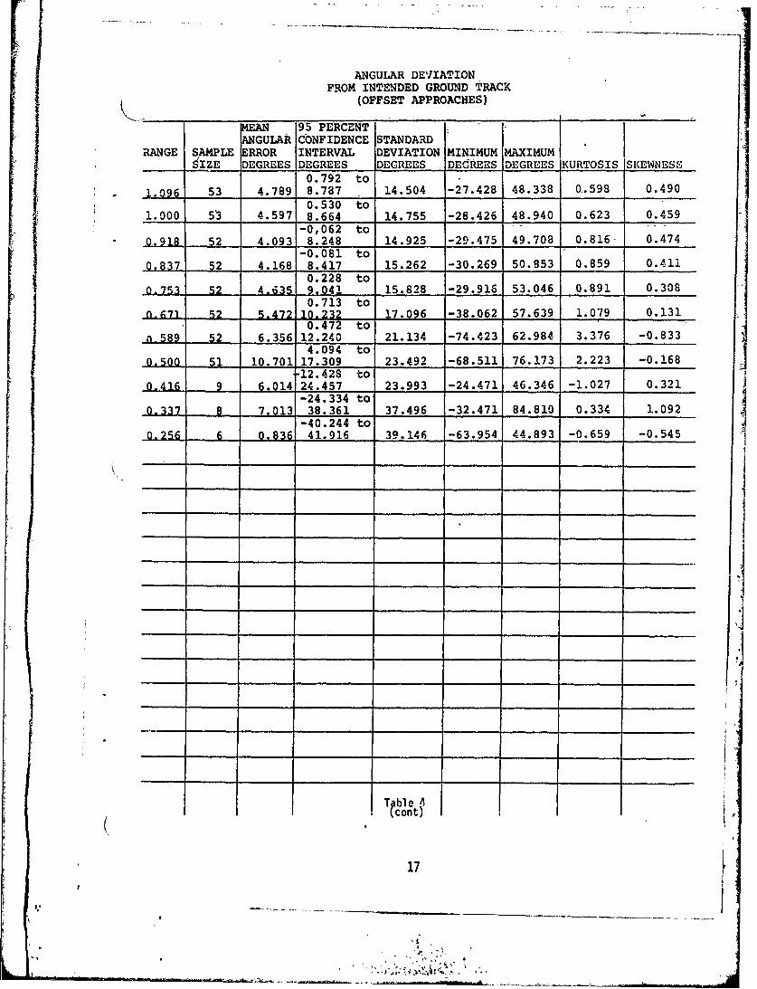
The average angular deviation of the offset approaches at ranges greater
than 1.261 nm was found to be between +50 and +7.60 (Table 4). The
average angular deviation of the straight-in approaches for all ranges
between2.753 nm and .501 nm was found to be between +40 and +5.60 (Table 5).
K The mean at 5 nm for the offset approaches was +7.3520 while that of the
straight-in approaches was only +0.0990. The means for both types of
approaches tended to be large within .589 nm since some aircraft had
initiated the missed approach turn and most of the turns were toward the
right.
A positive angular deviation indicates that the aircraft was right of
course when the angle was computed. The average angle of each of the
samples is positive,.which indicates that on the average, the aircraft
flew on the right side of the downwind final approach. It could be
reasonably expected that the averages would be near zero with some
positive and some negative values.
13
LAL

ANGULAR DI;VIATIO!FROM INTENDED GROLD TRACK
(ALL APPROACHES) _ _ _
MEAN -9,5 PERCENTANGULAR CONFIDENCE STANDARD
RANGE SAMPLE ERROR INTERVAL DEVIATION MINIMUM MAXIMUMSIZE DEGREES DEGREES DEGREES DEGREES' DEGREESr - KURTOSIS ISKWNE;S
1.248 to5.000 76 3.821 6.395 11.262 -27.154 35.850 0.911- -0'.045
3. 39b to4.000 99 5.730 8.064 11.703 -29.766 37-;715 , -1.158 -0.,285
3.342 to3.000 106 5.769 8.196 12.601 -30.494, 38.504 0.514 -0.217
3.281 to2.917 107 5.693 8.106 12.587 -30.253 38.310 0.476 -0.201
3.325 to2.836 106 5.762 8.199 12.654 -30.120 33.206 0.435 -0.219
3.459 to2.753 107 5.884 8.308 12.649 -30.077 38.203 0.428 -0.241
3.430 to " _ _
2.671 107 5.859 8.287 12.671 -30.040 38.265 0.408 -0.2443.396 to
2.589 107 5.833 8.271 12.717 -30.i102 38.410 6384 -0;2443.364 to
2.506 107 5.809 8.253 12.756 -30.252 38.1600 0.370, -0,.243.3.328 to
2.425 107 5.782 8.236 12.805 -30.504 38.977, 0.373 -:0.2423.288 to ,
2.342 107 5.755 8.221 12.869 -30.775 30.445 0.374 -0.2433.243 to
2.259 107 5.726 8.208 12.954 -31.075 40.070 0.375 j-0.1423.201 to I
2,177 1.7 5.702 8.-203 13.048 -31.380 40.615 0.366 -0.2373.180 to
2.094. 07 5.696 3.213 13.129 -31.647 41.266 0.360 -0.2273. 159 to
2.000 107 5.696 8.231 13.233 -32.097 41.886 0.341 -0.2192.572 to
1,918 103 5.171 7.769 13.297 -32.456 42.542 0.,406 -0.156i2.553 to
1825 103 5,17 .795 13, 4 13 -32.993 43.253 0.409 -0.1492.526 to
1.743 103 5.169 7,813 13,526 "... 388 43.881 0.402 -0.1382.489 to
.65-159 7828 13.658 -- 33.875 44,423 0.387. -0.1272.439 to
I.D I1 'A R13 7 A.A'3n 1-,793 ,34.368 44.793 0.367 -0.1202. 378 to
7 n*1 5-10l 7.928 11,441 -34.768 45.302 0,353 -0,1112.34.8 to
1 474 103 5107 7866 14.119 -35,269 45.887 0.341 -0.0982.406 to,_il1_.5,218 8.030 135 -35.629 46.547 0.340 -0.098
2.232 to1.260 103 5.061 .7.890 14.474 -35.846 47.084 0.2S9 -0.062
2.171 to1.177 103 5.034 7.89S 14.651 -36.126 47.700 0.270 -0.052
Table 3 (
14
'Ij
|,4
.' *1"

ANGULAR DZVIATIONFROM INTENDED GROUND TRAC.X
(ALL APPROACHES)
KEAN -95 PERCENTANGULAR CONFIDENCE STANDARD
RANGE SAMPLE ERROR INTERVAL DEVIATION MINIMUM MAXIMUMSIZE DEGREES DEGREES DEGREES DEGREES DEGREES KURTOSIS ISKEWNESS
2.068 to1.094 103 4.970 7.873 14.850 -36.415 48.339 0.255 -0.042
1.000, 102 4.936 7.914 15.158 -36.813 48.940 0.214 -0.048
1 4.646 to0.918 101 4.6781 7.709 15.356 -37.118 49.708 0.250 -0.029
1.605 to0.837 102 4.666 7.727 15.584 -37.452 50.853 0.284 " -0.029
1.792 to0.754 102 4.935 8.078 16.001 -37.791 53.046 0.319 -0.055
2.131 to0.671 102 5.435 8.739 16.818 -3L. 0;. 57.639 0.483 -0,103
2.154 to0.588 102 5.923 9.692 19. 190 -74.423 624.9844 2. -0.653
4.030 to0,500 101 8,167 12-305 20.57 18.11 7 .17 1.827 -0.087
-5.682 to0.416 19 6.762 19.205 25.817 -30.454 47.360 -1.262 0.180
-8 .671 to0.335 18 8.005 24.680 33.533 -3.224 84.810 -0.3I 0.649
-12.688 to0.254 16 7.650 27.987 38.167 -63.954 70.819 -0.791 -0.062
t " _ _ _ _ _ _ _
Table 3( (cont)
£1
I.
'I!

AiGULAR DLVIATIONFROM INTENDED GROUND TRACK
__ _ _ (OFFSET APPROACHES) _
MEAN 95 PERCENTANGULAR CONFIDENCE STANDARD
RANGE SAMPLE ERROR iNTERVAL DEVIATION MINIMUM MAXIMUM____SIZE DEGREES DEGREES DEGREES DEGREES DEGREES KURTOSIS SKEWNES.-;
4.002 to5.1000 39 7.352,10.702 10.335 -13.335 35.850 0.706. 0.749
4.504 to4.301 51 7.515 10.525 10.704 -13.594 37.775 0.685 0.6514.258 to
3.002 55 7.457 10.656 11.833 -16.707 38.504 0.102 0.430
2.917 56 7.279 10.444 11.817 -16.872 38.310 0.082 0.4474.230 to
2.837 55 7.444 10.657 11.889 -17.122 38.206- 0.029 n.3984.277 to
2.752 57 7.419 10.561 11.842 -17.445. 38.203 - 0.001 0.3804.208 to
2.671 57 7.356,10.504 11.864 -17.839 38.265 0.302 0.3674.121 to
2.389 57 7.286 10.452 11.930 -18.499 38.410 0.007 0.3504.029 to
2.507 57 7.208 10,387 11.982 -19.053 38,600 0.021 0.3373.936 to
2A24 57 7,132 10.328 12.045 -19,605 -38,977 0.059 0.3313.840 to
2.341 57 7.056 10.272 12.120 -20.318 39.445 0.104 0.3233.737 to °
2.259 57 6.979 10.221 12.219 -20.861 40.070 0.149 0.3203.640 to
2.177 57 6.915 10.191 12.346 -21.193 40.615 0.166 0.3223.562 to
2.095 57 6.869 10.176 12.463 -21.282 41.266 .0.186 0.3313.461 to
2.001 57 6.805 10.150 12.604 -21.393 41.886 0.185 0.3362.310 to
1.917 53 5.806 9.303 12.685 -21.835 42.542 0.516 0.4962_.12_ tO-
1.836 53 5.753 9.294 12.646 -22.190 43.253 0.527 0.5032.104 to
1.754 53 5.690 9.275 13.009 -22.660 3.881 0.537 0.5091.982 to
1.669 53 5.618 9.253 13.190 -23.082 44.423 0.531 0.3141.841 to
1.589 53 5.523 9.204 13.356 -23.571 44.793 0.514 0.5141.664 to
1.506 53 5.395 9.126 13.534 -24.313 45.302 0.522 0.5121.509 to
1,424 53j. 5.293 9.077 ' 13.729 -24.848 45.887 0.524 0.5131.344 to
J, . . 23 _ 9 -25.372 46.547 0.538 0.5201.170 to
1.261 53 5.063 8.955 14.123 -25.963 47.084 0.539 0.5140.998 to
1.178 53 4.942 8.886 14.309 -26.732 47.700 0.567 0.502
Table 4
16
ANGULAR DEVIATIONFROM INTENDED GROUND TRACK
(OFFSET APPROACHES)
MEAN 95 PERCENTANGULAR CONFIDENCE STANDARD
RANGE SAMPLE ERROR INTERVAL DEVIATION MINIMUM MAXIMUMSIZE DEGREES DEGREES DEGREES DEGREES DEGREES KURTOSIS SKEWNESS0. 792 to
1.096 53 4.789 8.787 14.504 -27.428 48.338 0,.598 0.490
0.530 to1.000 53 4.597 8.664 14.755 -28.426 48.940 0.623 0.459
-0,062 to0.918 52 4.093 8.248 14.925 -29.475 49.708 0.816- 0.474
-0.081 to,.837 52 4.168 8.417 15.262 -30.269 50.853 0.859 0.411
0.228 to0.753 52 4.,63 9.041 15.828 -29.916 53.046 0.891 0.308
0.713 to.671 52 5,472 -10232 17.096 -38.062 57.639 1.079 0.131
0.472 ton- 589 52 6.356 12.240 21.134 -74.423 62.984 3.376 -0.833
4. 094 to0L500 1 10.701 17.309 23.492 -68.511 76.173 2.223- -0.168
,12.428 to0,416 9 60.14 24.457 23.993 -24.471 46.346 -1.027 0.321
-24.334 to0.337 8 7Q13 38.361 37.496 -32.471 84.810 0.334 1.092
-40.244 to.256 6 0,836 41.916 39.146 -63.954 44.893 -0.659 -0.545
Tble .
(, cont)
17

* ANGULAR DEVIATIONFROM INTENDED GROUND TRACK
(STRAIGHT-N APPROACHES) ..... __
S AN, 9 5 P E R C E N T . . .. ..GU LR CONFiDENCE STANDARD
RANGE SAMPLE RROR INTERVAL DEVIATION MINIMUM MAXIMUMSIZE DGREES DEGREES DEGREES DCREBS DEdREES KURTOSIS ISKEWNE'(
.;-3.§10 to5.000 .37 0.099 3. 808 11.124 -27.1-54 19.605 -0.136 -0.590
0._200 -to4.001 48 3.834 7.467 12.51.3 -29.766 28.132 0.626 -0.801"0 .220 to .... .
3.001 -51 3.948 7.667 13.256 -30.494 30.0231, 0.232 -0.640'0.216 to
2.917 .51 3.952 7.687 13.280 -30.253 29.931 0..i99 0. 6280.206 to
2.835 51 3.949 7.693 13.310 -0,120 29.785 0.,173 -0.6200.321 to
2.753 50 4.134 7.946 13,416 -30.077 29.6r .179 -.n5.20.329 to
2.670 50 4.12 7.974 13.450 -300A0 29 -902.'- .. -'I -IL 6;ZAI0.344 to
2.589 50 4.177 8.010 13.487 -30.102 29.392 0.i44 1 2-0.6400.368 to .
2.506 50 4.213 8.058 13.529 -31252 29.285 0 6 -00.384 to2.425 50 4.243 .12 13.578 -30,504 29.1806 0.i35 -0.633
0.393 to2.343 50 4.271 8.149 13.645 -3167 29.17 0.125 -006462
.395 to .. . . I
2.259 50 4.297 8.198 13.728 -31.075 28.7311 '0.112 .634 i0,.397 to2.178 50 4.3191 8.241 13.800 ,-31.380 28514' ,0.103 -0.639
0 .422 to2.094 50 4.360 8.297 13.955 -31.647 28.277 0,094 -0.641
"0.468 to2.000 50 4.429 8.389 13.93,6 -32. 9)7 , 27.989 0,0(85 -0.643.
0.514 to1.918 50 4.496 8.479 14.015 -32,456 27.766 0.078 -0,64L.
0.555 to1.837 50 4.560 8.566 14094 -32 993 .27 ,885,1 0.094 -O.A5!
0. 593 to1.754 50 4.618 8.643 14.164 -.3.318 2.2a9. .OaL _n_#;9
0.620 to1.671 50 4.672 8.723 14.256 -33.875 28.713 0,095 -0.652
0.641 to1.590 50 4.723 8.806 14.366 -34.368 .29222 0.097 -0Q. 50
0.675 to1.508 50 4.7931 8.91.1 14.490 -34.763 29.902 0-092 -0-641
0.744 to1.423 50 4.909 9.075 14.657 .- 15-299 30-848 9 0 o
0. 986 to1.341 49 5.256 9.525 14.865 -35.6g9 31.4R7. o.,Ir -ogs
0.802 to
1.259 50 5.059 9.316 14.980 _-35.846 -3-1 U3 0.0 A -n.5750.826 to
1.177 50 5.132 9.438 15.150 -36.2 31'.96 024 -S.4-
Table 5
S(
11
7"4
V.t .*

ANGULAR DEVIATIONIFROM INTENDED GROUND TRACK((STRAIqHT-IN APPROACHES)
. -EAN 95 PERCENT 4A-GULAR CONFIDENCE STANDARD
RANGE SAMPLE ERROR INTERVAL DEVIATION MINIMUM MAXIMUMSIZE DEGREES DEGREES DEGRETES DEGREES DEGREES KURTOSIS iSKEWNES.S
0.799 to1.094 50 5.162 9.526 15.3;4 -36.413 32.304 -0.008 -0.523
U. 736 to0.999 9 5.304 9.822 15.28 z-36.813 32.706 -0.068 -0.511
0. 722 to -0.918 49 5.298, 9.875 ]15.933 -37.118 33.494 -0. 099 -0.484
0. 622 to0.837 50 5.184 9.746 16.052 -37.452 34.159 -0.117 -0.431
0.606 to0.755 so 5.248 9.890 16.333 -37.791 34.853 -0.159 -0.403
0.650 to0.671 50 5.395 10.141 16.698 -37.929 35.828 .-0.209 -0.364
0,5880. 602 to.58 50 5,473 10.344 17.139 -37. 972 36.603 -0.263 -0.314-
0. 501 to0.01 50 55310.644 1780 -3.4 40,595 -0.355 -0.216
13.053 to0-4106 in 7-434 27,922 28.640 -30.454 47.360 -1.433 0.081
"14.143 to2-.31 i0 879R 31.7,3 32.07f6 -34224 55.613 -1.357 0.123
16.216 to0..D2.5 fl 1.738 3.6939.077 -40.430 70,819 -1.201 0.174
(cont)(19
__ _ __|_ _ _ _ __ _ _ __ _ _ _ __ _ _ _ __ _ _ ,__ _ _ _ _____ ___r, __ ___.. . ._
___ |%I
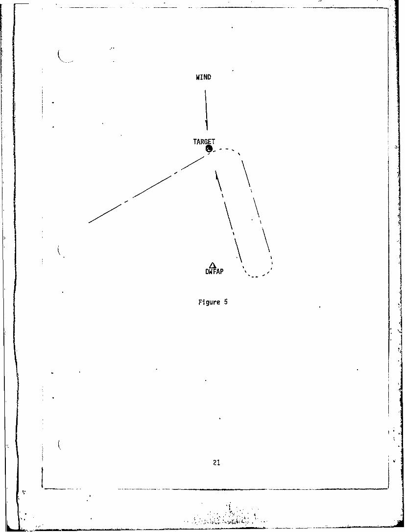
The bias observed in the data-may have been caused by a combination of
procedure and technique used to reach the downwind- final approach point.
The 6verhead procedre rbquired the- crew to fly directly over the target
0 0rig and then take up a course 10 12 from the reci.procal of the
downwind final approach course. Ideally, the- helicopter would leave the
target rig on the 100 - 120 offset course as in- Figure 2. In practice,
the turn to the offset -heading, coupled with the inaccuracies of
determining when the aircraft was directly above the target rig, resulted
in a flight path more like Figure 5. Although no statistical tests were
performed to verify this conjecture, evidence does exist which supports
it.
Of the 58 offset approaches, 48 turned right during the overhead maneuver
while only 5 turned left. The remainder either flew over the target rig (already on the outbound course or the overhead portion of the data was
missing. Of the 51 straight-in approaches, 31 turned right during the 1
overhead maneuver while only 3 turned left. Eleven of the straight-in
approaches used the arcing entry which was always initiated from left of
theadownwind final approach course. The remainder of the straight-in
approaches either flew over the target rig already on the outbound course
or the overhead portion of the data was missing.
20
~I 1________________________________________
WI ND
TARGET
DWFAP * \II
Fi gure 51
21

The proportion of right turn entries onto the outbound leg is higher for
the offset approaches than for the straight-in approaches. Each of the
arcing entries was performed prior to a straight-in approach; The bias
of the offset approach data is larger (indicating the'flights were on
the average farther rightof course) than the bias of.'thestraight-in
approaches. Therefore, it appears that, theoverhead turning,,maneuyer
tends to adversely, affect the accuracy of reaching.,the Downwind.FinAl
Approach Point (DWFAP).
Other factors may also have contributed to the track bias. The offset angle
used in the overhead maneuver may have been too large, for, the speeds and
distances flown causing the heicopter to be right of course at, the DWFAP.
The dead reckoning methodof determining the start, point of the,.standard
rate turn onto the downwind final approach course could also contribute to(
the error in reaching the DWFAP. Finally, since the crewmembers, were
inclined to home toward the target rather than seek.the proper approach-
course, the error in reaching the do,nwind final approach point was
carried through the entire flight. This last point will bediscussed in
more detail in later paragraphs.
The standard deviations of the angular deviations are also presented in
Tables 3, 4, and' 5. The standard deviati,,:rs for All approaches, Offset
approaches, and Straight-In approaches are very similar in size, all
being about 100 - 120 at 5 nm-and then stealiiy increasing to 140 - 150
at 1 nm. This similarity of standard deviations is to be expected since
(22
I.I
t • 1'
() ~the Offset approach procedure and the Straight-In approach procedureare identical to the 1 nm point.
It is often possible to combine angular data collected at different
ranges into one sample so that a probability density curve may be
found which fits the sample data with a high degree of confidence. This
procedure requires the samples be statistically from the same population
and be formed independently.
The Spearman rank correlation test was used to determine if the
samples could be considered to be independent. The Spearman test was
chosen because it is a nonparametric test requiring no assumptions
about the populations from which the samples are drawn. The test
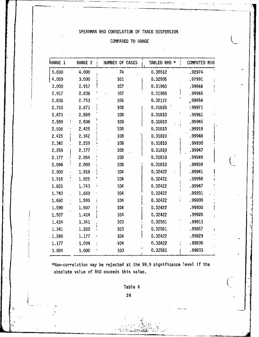
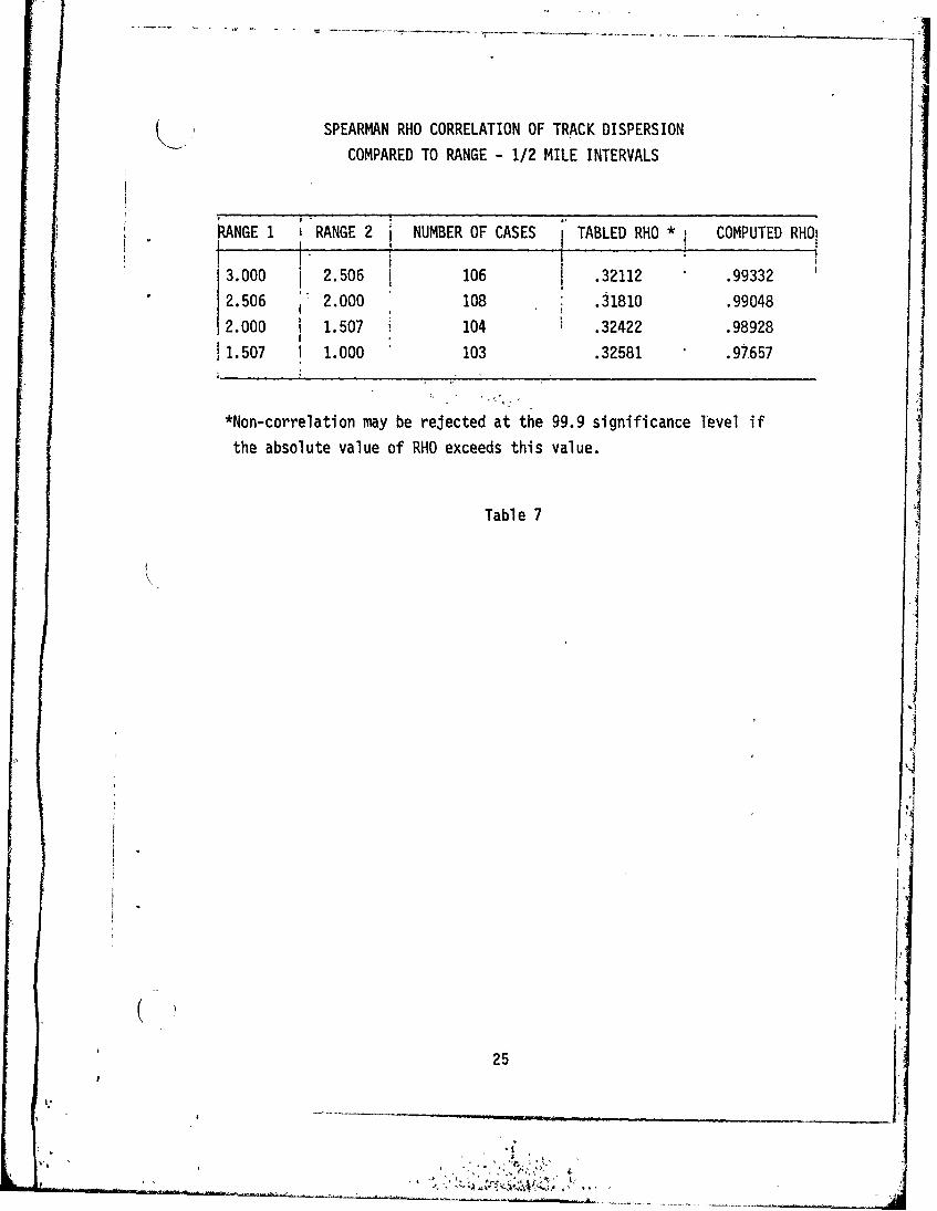
results are shown in Tables 6 and 7. The tables show that correlation
between samples at 500 foot intervals, half-mile intervals, and one mile
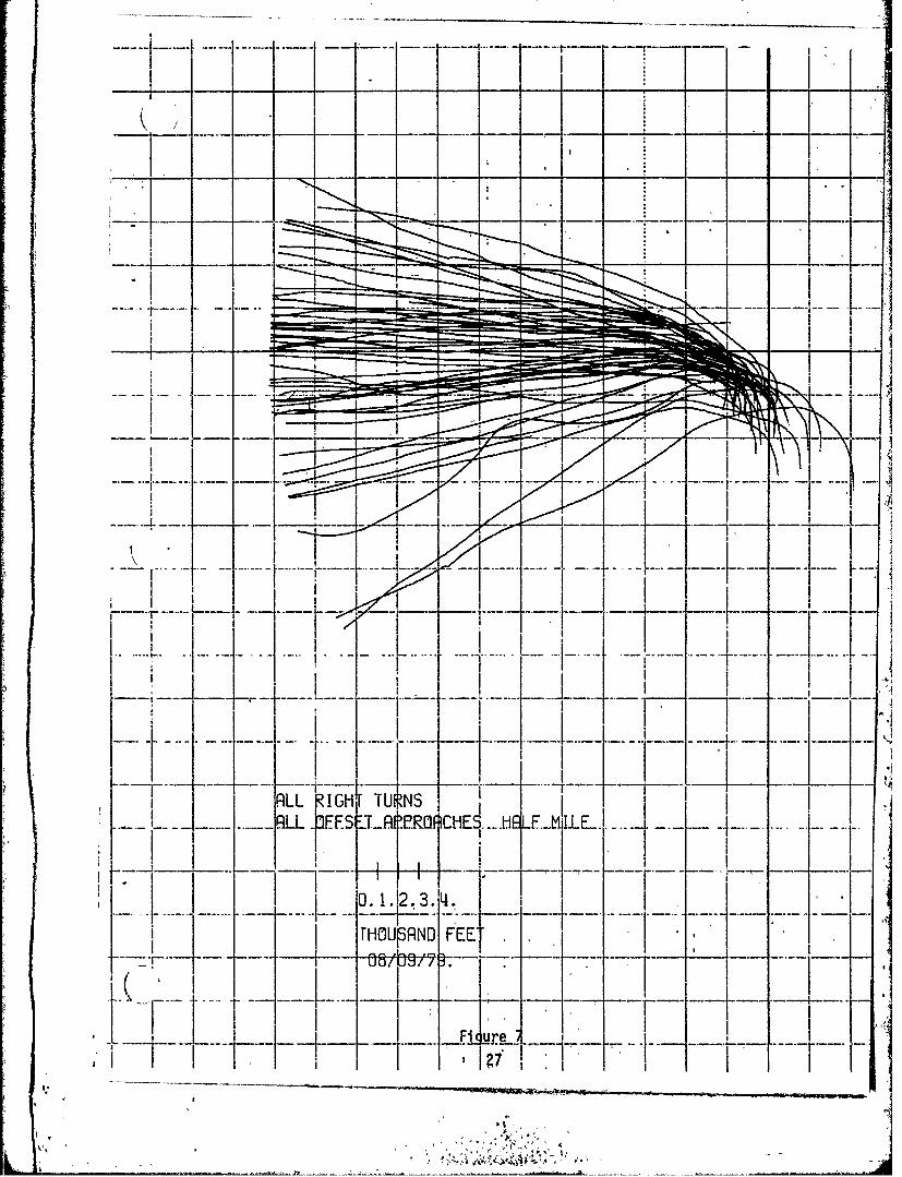
intervals were all highly significant. Thi.s means that the aircraft paths,
as seen in the composite graphs (Figures 6, 7, 8, and 9), are not crossing
one another very much. They are maintaining their relative positions from
range to range. When aircraft are attempting to follow a course such as
an ILS localizer, the paths cross each other often, and if the range interval
width is reasonably chosen, the aircraft position at one range will be
independent of its position at another. Thus, the high correlation is an
indication that the crewmembers were homing to the target rather than
following the predetermined final approach course. Thus the error in
reaching the DWFAP is retained throughout the flight.
23
I°"
,I
SPEARMAN RHO CORRELATION OF TRACK DISPERSION
COMPARED TO RANGE
!RANGE 1 RANGE 2 NUMBER OF CASES TABLED RHO * COMPUTED RHO
5.000 4.000 74 0.38512 .92974
4.000 3.000 101 0.32905 .97991
3.000 2.917 107 0;31960 .99946
2.917 2.836 107 0.31960 .99965
2.836 2.753 106 0.32112 *99954
2.753 2.671 108 I 0.31810 -.99971
2.671 2.589 108 0.31810 .99961
2.589 2.506 108 0. 1810 .99945
2.506 2.425 108 0.31810 .99919
2.425 2.342 108 0.31810 .99948
2.342 2.259 108 I O31810 I .99930
2.259 2.177 108 J 0.31810 , .99947
2.177 2.094 108 0.31810 .99949 I
2.094 2.000 " 108 '0.31810 i .99939 (2.000 1.918 104 0.32422 .99941 I1.918 1.825 104 0.32422 .99958
I'1.825 1.743 104 0.32422 .99947
1.743 1.660 104 0.32422 .99931
1.660 1.590 104 0.32422 .99900
1.590 1.507 104 0.32422 .99930
1.507 1.424 104 ' 0.32422 .99926
1.424 1.341 , 103 0.32581 .99911
1.341 1.260 103 0.32581 .99857
1.260 1.177 104 0.32422 .99829
1.177 1.094 .104 0.32422 .99836
1.094 1.000 103 0.32581 1 .99833
*Non-correlation may be rejected at the 99.9 significance level if the
absolute value of RHO exceeds this value.
Table 6
24I.
(SPEARMAN RHO CORRELATION OF TRACK DISPERSION
COMPARED TO RANGE - 1/2 MILE INTERVALS
RANGE 1 RANGE 2 NUMBER OF CASES TABLED RHO * COMPUTED RHOI I
3.000 12.506 I 106 I .32112 .993322.506 2.000 108 .31810 .99048
2.000 1 1.507 i 104 .32422 .98928II1 1.507 I 1.000 103 .32581 .97657
*Non-correlation may be rejected at the 99.9 significance level ifthe absolute value of RHO exceeds this value.
Table 7
\,i
I
j
25
LE
'V
V. -
,_ i . . . 2 VJI' ,

IZ-~~ ----
.. :-7 I
RL IH TURNS
4..L....--1*D EE
UO wof1* 37t~
-1-- -I-S: - -IH -.H - ---
1. . 2- 3.4
MOill---FEE 08'TU,-1II1 7

LL 1 G-TU
RLL IR G IN-FIPqCES- QIIIkKIF
IN g

I [I............ I
I. ~ ~ ~ 0 1.~**~ 3.'~-ITHO ''I E", i E
I I I2i]I
The samples were not c6mbined, but tests for normality using the sample
skewness and kurtosis were conducted. The tests indicate the assumption
that samples are from ormal populations cannot be rejected at the 5
percent level. The sample means plus or minus two standard deviations
were used to prepare Figures 10, 11, and 12. The probability that a
number drawn from a normal population is within two standard deviations
of the mean is about 0.95; thus at each range the probability of being
within the envelopes pictured on the graphs is about 0.95,.
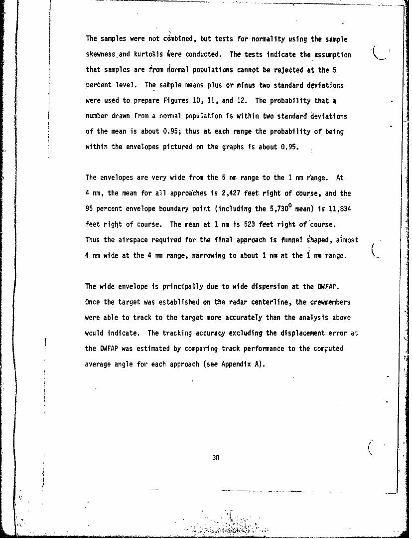
The envelopes are very wide from the 5 nm range to the 1 nm range. At
4 nm, the mean for all approaches is 2,427 feet right of course, and the
95 percent envelope boundary point (including the 5,7300 mean) is 11,834
feet right of course. The mean at 1 nm is 523 feet right of'course.
Thus the airspace required for the final approach is funnel ihaped, almost
4 nm wide at the 4 nm range, narrowing to about I nm at the I nm range.
The wide envelope is principally due to wide dispersion at the DWFAP.
Once the target was established on the radar centerlfne, the crewmembers
were able to track to the target more accurately than the analysis above
would indicate. The tracking accuracy excluding the displacement error at
the DWFAP was estimated by comparing track performance to the computed
average angle for each approach (see Appendix A).
30(
30

us
CC
LV
al:QeJ
ElU _ELL ___ L
U-EJ IL. M LUJ
I-. 2 Qn Lii
LU j
LU0Dz
cr..
00
lW'N'NOII.HIA 0 \AOUK1 SSO D
31

uD
cK-
0D 0 /
M LU Q- ) IL )I: > C> 1- a1
0zz ci: z~LO .LL -
0~
c~r1-4=
LUJ
IW*N'NOIJiHIAD0 N38i SGONJC
_______ 32 _ _ _ _ _ _ _ _ _ _ _ _ _ _ _ _ _ _ _ _ _ _ _ _ _

cLr_
oz
zCCLU z
a:- I>J F-
X*L a-. -.-
U)LL C MLL1L- C/)-I > CCI > t" LL
a-
F-
LU -
I - W'N'OII.IA~O ~ SS&D33) VcI 'I
I' A:CYI
0. 4 ~

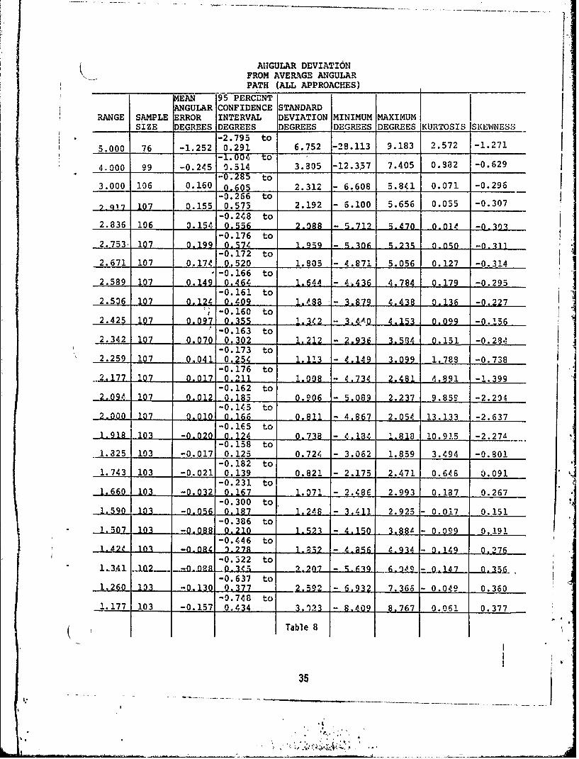
The stat.lstfcs for the average course, are presented fr TaIe! 8.v-9,, sold
The mean angular deviation fs- now' muc h closer to, zro,
The-,means of alil: approaches are within 0 of 00 for all ranges frew
I nm to, 1, nm., The means of the. straght-in approaches" are wfthfnf 0,70
of 0" for' al ranges from 3 nm, to, I nnr. The eans of the offst' appr'oach'es0, ' 0
are. withn', T..25 of 0 for all ranges fwrom 3 nm to 1 nm, The', means of
al.,approaches and. the Straight-i'n approaches- art, negatite atV 4 nm and'
5' nm while' the' means- of the offset approaces' 'are positive. The meant
at ranges- Tess than. I na increase refTectingT the mtssed approach turns.
The means for" the' offset approaches at ranges; less: than i' nnt do not
approach the 150 offset angTe sfnce there was a, mfxture of lieft tnd- right
offsets&
tHThe dlffference" i.n, signs'- of the means, a 4 m and i w for the: offset and
straight-tn approaches provides, further evidenc that more right hand
procedure turns were' used in' the offset approaches, than, in the straight-in
approaches'. It also, shows that many atrcraft are! still turnfng at 5, nm
and. 4. nm but, have established a course, to the target. by W m.,
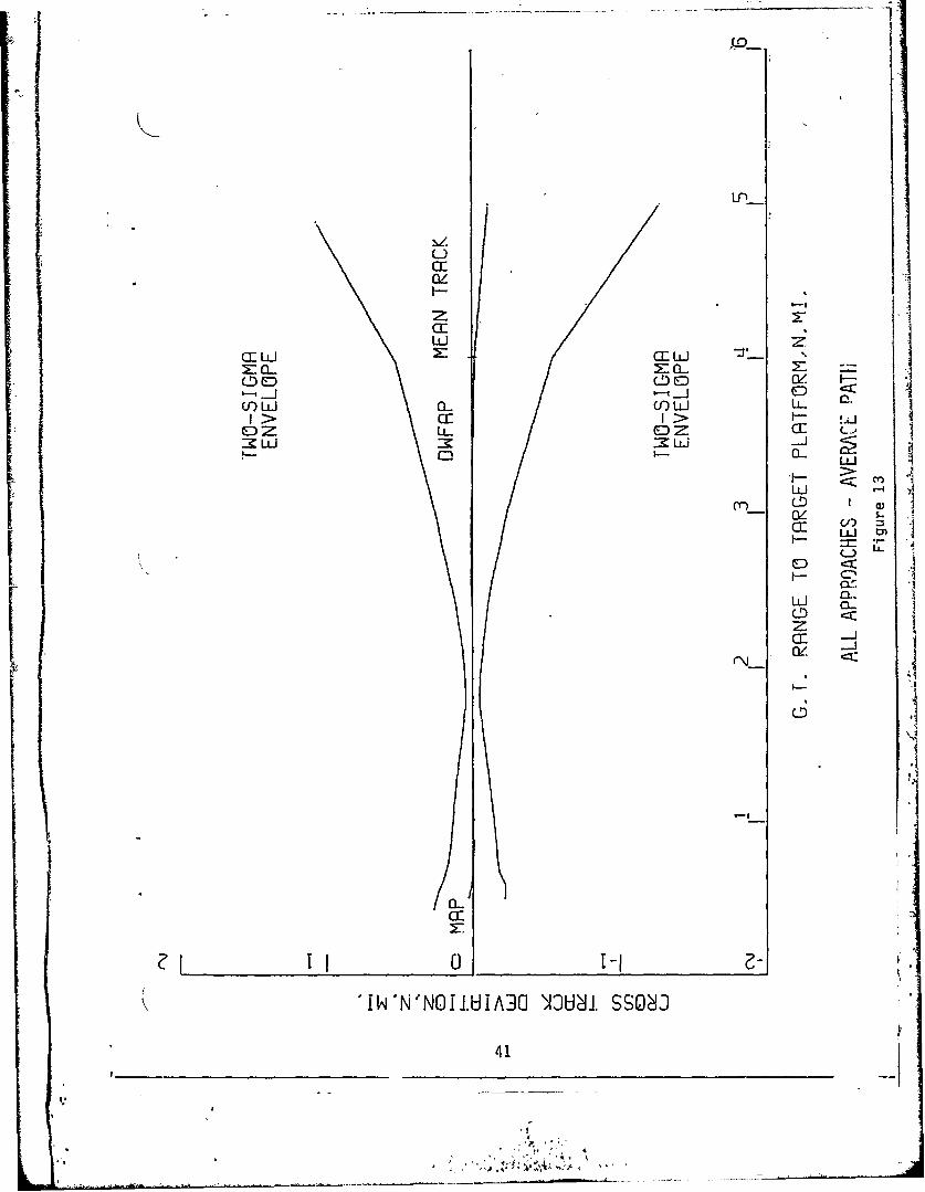
The standard deviations about the average path are much smaller than the
standard deviations about the intended path. The, starida'd deviations for
all' approaches are between, .7240 and' 4.1069" for the ranges f0om' 1 nm to
3 nm. The standard deviation at 5 nm 1'.5 only 6.7520. A two standard
deviation envelope about the- mean ft shown i'ni Figure 13'.,,
34
*1.,
'a
ANGULAR DEVIATIONFROM AVERAGE ANGULARPATH (ALL APPROACHES)
MEAN 95 PERCENTANGULAR CONFIDENCE STANDARD
RANGE SAMPLE ERROR INTERVAL DEVIATION MINIMUM MAXIMUM
SIZE DEGREES DEGREES DEGREES DEGREES DEGREES KURTOSIS SKEWNESS-2.795 to
5.000 76 -1.252, 0.291 6.752 -28.113 9.183 2.572 -1.271-1. 004 to
4.000 99 -0.245 0.514 3.305 -12.357 7.405 0.982 -0.629
3.000 106 0.160 0,605 2.312 - 6.608 5.841 0.071 -0.296-0.266 to
i:q67 107 0.155 0.573 2.192 - 5.100 5.656 0.035 -0.307
-0.248 to2.836 106 0.154 0.556 .547n 0.014 -0,303
-0.176 to2.733 107 0.199 0.57Z 1.959 -1-*30 5.35 0.5 -,.311
-0.172 to
2.671 107 0.174 0.520 1.803 - 4.871 5.056 0.127 -0.314, -0.166 to
2.589 107 0.149 0,46 . 1.544 - C436 4.784 0.179 -0.293-0.161 to2.536 107 0.1 ,0409 1.483 3.8791 ..438 0.136 1-0,227
. -0.160 to2.425 107 0.097. 0355 1.3t2 - 3. 4 4.153 0.099 -0.156
-0.163 to2.342 107 0 0.302 1.212 -2.936 3.5 4 0.151 -0.284
-0.173 to2.259 107 0.0 ,025t, 1.113- 4.1491 3.099 1.789 -. 3
-0.176 to2.177 107 0.017 0.211 .008 -4.,734 2.481 d.191 -1.399
-0.162 to2.094 107 0.012 0,183 0.906 -5,089 2.237 9.853 -2.204
-0.145 to2.000 107 0.010 0.166 0.811 - 4.867 1.059 13.133 -2.637
-0.165 to1.793 103 -0.020 0.124 0.738 - 4.134 1,18 0.915 -2.27
-0.158 to-.325 103 -0.017 0.125 0.724 - 3.062 1.859 3.494 -0.801-0. 182 to
1.743 103 -0.021 0.139 0.821 -2.175 2.471 0.646 0.091-0. 231 to
1.660 103 -0.032 1QI7 1.071 - 2.486 2.993 0.187 0.267-0.300 to
1.590 103 -0.056 0.187 1.2i,8 - 3.411 2.925 - 0.017 0.15107 13 - -0.- 386 to
1.507 1 .210 1.523 - 4.150 3.8 - 0.099 0.191-0.446 to
1.421 InI -0-ni 1,77 1al.a2 - 4R.56 4,934 - 0.149 Q.276-0.522 to
13A1 I.Q - --2 ---.... - _ 0 -; 2..207 - S9 _...9!i -0..17_ . .AxL.-0.637 to
-.260 103 -0.130 0,377 2.592 - 5.932 7 -66 0.049 0.360-0.748 to
1.177 103 -0.157 0.434 3,123 - 8.409 8.767 0.061 0.377
( Table 8
35
35
I..
'I.. .'4]

ANGULAR DEVIATION, . FROM AVERACE ANGULAR
PATH (ALL APPROACHES) QMEAN 95 PERCENTANGULAR CONFIDENCE STANDARDRANGE SAMPLE ERROR INTE RVAL DEVIATION MINIMUM MAXIMUM
SIZE DEGREES DEGREES DEGREES DEGREES DEGREES KURTOSISISKEWNESS
-0.906 to103 -n-22n 0.463 3.506 -10.065 10.269 0,201 0.373
1"1.118 to1.000 102 -0.311 0.495 4.106 -11.820 12.094 0.329 0.392
-1.311 to0.918 101 -0.386 0.538 4.61 -!3,381 13.513 0.373 0.387-1.'4.07 to "0.837 102 -0.343 0.722 5.419 -15A21 A9 0.377 0,294
-1.334 to0,754 102 -0Q.74 1..6 6.A1i -A97 if'.47i 0,472 0.107i -1.145, t6 •0,671 102 0-426 1-997 7.gOg -24.718 19.048 0.983 -0.193
-1. 344' to -0.588 102 0.915 3.173 11.497 -59.109 25.869 6.780 -1.458
0.052 o
0.500 101 2.958 5.,86 14.719 -63.635 57..837 4.800 -0.393-3.553 to.
0.416 19 5.967 15.487 19.751 -27.,587 48.525 -0.340 0.197-7.330 to
0.335 18 7.049 21.428 28.914 -36.808 80.070 0.648 0.507-9.472 to
0.254 16 8.096 25.664 32.970 -67.010 54.650 0.133 -0.736
Table 8(cont)
36

ANGULAR DEVIATIONFROM AVERAGE .ANGULAR PATH
(OFFSET APPROACHES)
MEAN 95 PERCENTANGULAR CONFIDENCE STANDARDRANGE SAMPLE ERROR INTERVAL DEVIATION MINIMUM MAXIMUMSIZE DEGREES DEGREES DEGREES DEGREES DEGREES KURTOSIS ISKEWNESS
-1.475 to.5.000 39 0.105 1.685 4.873 -11.163 9.183 - 0.403 -0.351
-0.406 to4.001 51 0.490 1.385 3.183 - 5.950 7.405 - 0.502 0.062
0.119 to3.002 55 0.682 1.244 2.082 - 3.640 5.841 - 0.080 0.074
0.128 to2.917 56 0.659 1.190 1.984 - 3.836 5.656 0.065 0.032
0.154 to2.837 55 0.668 1.183 1.903 - 3.940 5.470 0.126 -0.013
0.210 to m2.752 57 0,687 1,165 1.799 - 3.941 5.235 0.161 -0.043
0.184 to2.671 57 0.624 1,064 - 1.660 - 3.880. 5.056 0.449 -. 80.156 to
2.aai 57 0-55 0-954 1.50i - 3.714 1,784 0.698 -0.0860.113 %o
2.507 57 0.476 0.839 1.369 - 3.545 4.438 0.859 -0.0740.073 to
2.424 57 0.400 0.727 1.233 - 3.169 4.153 1.008 -0.0300.031 to
2.341 57 0.324 0.618 1.105 - 2.839 3.584 1.447 -0.335-0.026 to
2.259 57 0.247 0.520 1.028 - 4.149 3.099 5.155 -1.211-0.066 to
.. .17 57 0.184 0.433 0.940 - 4.734 2.A81 11.800 -2.406-0..098 to
2.095 57 0.137 0.372 0.886 - 5.089 1.932 19.627 -3.587-0.146 to
2.001 57 0.074 0.293 0.828 - 4.867 1.524 20.709 -3.796-0.234 to
1.917 53 -0.044 0.165 0.759 - 4.184 1.297 15.427 -3.272-0.306 to
1,836 53 -0.098 0.110 0.753 - 3.062 1.824 4.040 -1.140-0.402 to
.75A 53 -0.,161 0.800 0.875 - 2.175 2.471 0.887 0.099-0.528 to
69 53 -0.33 0.061 1.069 -2.486 2.993 0.632 0.356-0.678 to
...a 53 -0.329 0.021 1.268 - 3.411 2.925 0.180 0.122-0.867 to
-.1506 53 -0.456 -0.045 1.490 - 4.150 3.157 - 0.079 0.076-1.039 to
1-.24 S3 -0.558-Q,.077 1.746 - 4.856 3.741m- 0.175 0.127-1.225 to
S1.,3A1.2_.._.ia_- 667 -00 .=ii0 23 -. 639 4.405 - 0.093 0.228-1.442 to
1.261 53 -0.788 -0.135 2.371 - 6.932 4.935 - 0.052 0.160-1.663 to
1.178 53 -0.909 -0.155 2.735 - 8.409 5.557 0.121 0.155
I Table 9
37

- ANGILAR DBLViATIONFROM AVERAGE ,kA,1.6L~ PAsTH
(OFFSEt APPR.ACHES)
MEAN 95 PERCENTANGULAR: CONFIDENCE STANDARD
RANGE SAMiPLE ERROR INTERVAL DEVIATION MINIMUM MAXIMUM_ SIZE DEGREES DEdREES DEGREES EDEGREES.DEGREES KJRTOSISISKEWNESS
-1.926, to I-096 33 -1.061 -0.197 3.135 -10.065- 6.194 '0.344 1 0.134
72.258 to1.000 53 -1.254 -0.250 3.6-43 -11.820 7.245 -0. 561 0.171
-2. 584 to_0.918 52 -1.414-0.243 4.204 -13.831 9,440 .0,664 0.217
-2.740 to0.837 52 -1.338 0.063 54033 r-15.421 -1-1.682 :0.504 0.127
-2.634 to I0.753 52 -0.872 0.891 .6 1329- -18.897 1-4.884- --0.605 -0.-106
-2.423 to0.61 52 -0.034 2,354 8579 -24.718 19,048 1. 069 -0.510
-3.013 to_.339 52 0.850.' 4-71-3 1.17 5i 25,869 5.-722 -1.740
-0.299 to,.))Q C00 5] 7A7 9-A74, 19.0RA -93-635 57,837 I3.R13 -0.738
-11.528 toii-4ir& 9 5809. 23,146 22.555 -22,780, 48.525 L-0.382 0.505
-24.264 .to0.337 8 6.516 37.295 36.817 1-36.808 80.070 .0.99 0.757
-35.940 to
0 .256 6 4 .231 44.401 38.279 -67.010 41.11 0.166 -1.122
k?
Table 9(cont)
___8
_ _ _ K

IANGULAR DEVIATION
FROM AVERAGE ANGULAR PATH(STRAIGHT-IN APPROACHES)
MEAN 95 PERCENTANGULAR CONFIDENCE STANDARD
RANGE SAMPLE ERROR INTERVAL DEVIATION MINIMUM MAXIMUMSIZE DEGREES DEGREES DEGREES DEGREES DEGREES KURTOSIS ISKEWNES,-5.385 to "
S 37 -2.682 0.023 8.112 -28.113 9.131 1.291 -1.115
-2.264 to4.001 48 -1.026 0.213 4.266 -12.357 6.862 0.489 -0.718
-1.087 to3.O01 51 -0.402 0.282 2.434 - 6.608 4.537 -0.348 -0.397
-1.044 to2.917 51 -0.399 0.246 2.293 - 6.100 3.942 -0.456 -0.409
-1.007 to2.835 51 -0.402 0.204 2.153 - 5.712 3.403 -0.530 -0.402
-0. 927 to2.753 50 -0.358 0.212 2.003 - 5.306 2.895 -0.520 -0.432
-0.863 to70 -0.339 0.184 1.842 - 4.871 2.798 -0.520 -0.410
-0.794 to2.589 50 -0.314 0,166 1.689 -'4.436 2.675 -0.526 -0.346
-0.713 to.2.5;06 5 -0.278 0.156 1.529 - 3.879 2.451 -0.611 -0.233
-0.643 to2-425 S -5. Q-147.24 1,390 - 3,440 2.306 -0.690 -0.118
-0.582 to2.343 50 -0.221 0.141 1.273 - 2.936 2.378 -0.664 -0.110- -0.527 to2.259 50 -0.194 0.138 1.169 - 3.290 2.431 -0.028 -0.304
-0.473 to2.178 50 -0.,172 0.129 1.059 - 3.274 2.397 1.128 -0.587
-0.392 to2.094 50 -0.132 0.128 0.915 - 3.188 2.237 2.432 -0.891
-0.288 to2.000 50 -0.062 0.163 0.794 - 3.198 2.054 4.386 -1.218
-0. 200 to1.918 50 0.0051 0.210 0.721 - 2.881 1.818 4.599 -1.030
-0.127 to1.837 50 0.069 0.265 0.689 - 2.295 1.859 2.174 -0.291
-0.084 to1.754 50 0.127 0.337 0.740 - 1.651 2.065 -0.140 0.326
-0.082 to1.671 50 0.181 0.443 0.923 - 1.366 2.322 -0.647 0.399
-0.101to
- 1.590 50 0.232 0.565 1.170 - 1.871 2.892 -0.529 0.348
-0.117 to1.508 50 0.30A 0.721 1.474 - 2.342 3.884 -0.446 0.374
-0.106 to1.423 50 0.41E 0.943 1.845 - 2.885 4.934 -0.470 0.382
-0.107 to.1.341 49 0.53E 1.183 2.246 - 3.545 6.049 -0.496 0.372
-0.137 to1.259 50 0.569 1.323 2.657 - 4.204 7.366 -0.430 0.416
-0.250 to1.177 50 0.64] 1.531 3.133 - 5.105 8.767 -0.359 0.414
Table 10
39

ANGULAR DEVIATIONFROM AVERAGE ANGULAR PATH
(STRAIGHT-IN APPROACHES)
-. MEAN 95 PERCENTANGULAR CONFIDENCE STANDARD
RANGE SAMPLE ERROR INTERVAL DEVIATION MINIMUM MAXIMUMSIZE DEGREES DEGREES DEGREES DEGREES DEGREES. KURTOSISIS_EWNS_
-0.376 to
.. Q9A 50 0.671 1.719 3.685 - 6.521 10.269 -0.255 0.390-0.545 to
..0.999 .49 0,709 1.963 4.365 - 8.623 12.094 -0.138 0.367-0.718 to
... 0.918 49 0,704 2.126 4.952 -10.330- 13.513 -0.054 0.357-0.916 to
f.83.7 .50 0,693 2.301 5.659 -12.740 14.997 0.092 0.327-1.080 to_. 7 _c C; Sn 0.756 2-S93 6,461 -15.068 16.479 0.163 -0.305 .
-1.200 to...0-67i. 50 0.904 3.008 7.403 -16.958 18.769 0.291 0.390
-1.431 to
.500.588 0.982 3.395 8.491 -19.633 22.411 0.437' 0.444-1.770 to
_0.501 50 1,091 3.952 10.066 -23.265 29.135 0.813 0.591-6.846 to
0,4161 1i0 6,109 19,065 18.111 -27.587 31.211' -0.567 -0.325-8.907 to
0.334 10 7.476 23.858 22.901 -35.504 39.468 -0.530 -0.350-11.999 to
0.254 10 10.415 32.829 31.332 -47.344 54.650 -0.563 -0.274
Table 10(cont)
40
__ _ _
6@."
LL)
CE -fX:C- L
Zu LU z 0
V)*- Q U LJ o -
ED Z: U-0: CCa li-' __ ZLU
M1LU '-
w -
LU
z
0.
JNWN'NOIJ.HIADO ' A3UW. SS08LJ
41

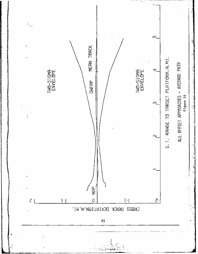
The standard deviations of the Offset approaches and Straight-In approaches
are also much smaller than the corresponding standard deviations from the
intended path. Two standard deviation envelopes for the offset approaches
and the straight-in approaches are shown in Figures 14 and 15.
The small standard deviations from the average angular path indicate that
once established on target the pilots flew relatively straight to the
target. Thus the wide envelopes found for the intended path are indications
of the large inaccuracies associated with reaching the DWFAP. If the DWFAP
could be accurately found by the crew, then the lateral airspace requirements
could be drastically reduced.
Although the error induced by the dead reckoning method for reaching the
DWFAP represents a large portion of the error observed when the aircraft (flew the final approach, there are other sources of error which should
be considered. Two other primary sources of error are the radar and crew.
The radar, because of technological considerations, may induce error, and
the crewmember, because of human considerations, may induce error.
Data to establish these two components of error were obtained (see Appendix
A) by photographing the radar display at regular intervals. To obtain
radar error from these photographs, the aircraft position indicated by
radar was compared to the actual position of the aircraft. In addition,
the difference in position given by the radar compared to the position
where the aircraft should have been was used as the measure of the human
error.
(42
'I
U)'
NZ
WI-
zULJ
CE LLJ CC LU
z. cl 2, - I
EZ ED Zac:a Ld -KLU -
L-.-
c i- 0 cri s
c:F- . LL-
C-
al: 6:wJ
CD -Jj1
I0
1IW'N'NOIJ.HIA O NOHW. SS0 3
43

L)
CC
aCE LU CE LJ5-; Q. y_ a. X: LU
LL) (EDr 0 )1 (CO LU U. C.LIJ ILI > CcIa:F
0 -L ED Z CC
uLi U.)
- LU
a: s-
ED LL.~
H-
LD
CLI2: =
x" ~
0
IW'N'NOIJ.UIA9O OHKJ SSO(
AA
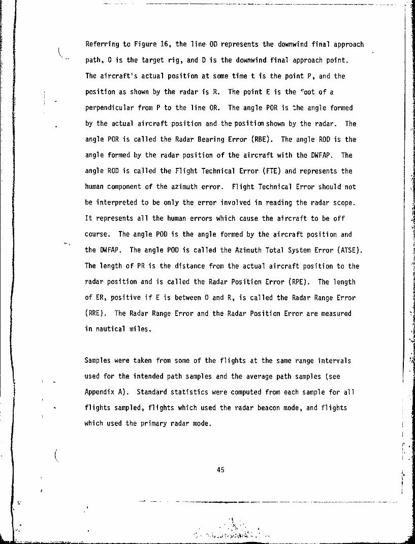
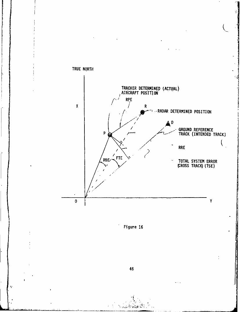
Referring to Figure 16, the line OD represents the downwind final approach
path, 0 is the target rig, and D is the downwind final approach point.
The aircraft's actual position at some time t is the point P, and the
position as shown by the radar is R. The point E is the root of a
perpendicular from P to the line OR. The angle POR is the angle formed
by the actual aircraft position and the position shown by the radar. The
angle POR is called the Radar Bearing Error (RBE). The angle ROD is the
angle formed by the radar position of the aircraft with the DWFAP. The
angle ROD is called the Flight Technical Error (FTE) and represents the
human component of the azimuth error. Flight Technical Error should not
be interpreted to be only the error involved in reading the radar scope.
It represents all the human errors which cause the aircraft to be off
course. The angle POD is the angle formed by the aircraft position and
the DWFAP. The angle POD is called the Azimuth Total System Error (ATSE).
The length of PR is the distance from the actual aircraft position to the
radar position and is called the Radar Position Error (RPE). The length
of ER, positive if E is between 0 and R, is called the Radar Range Error
(RRE). The Radar Range Error and the Radar Position Error are measured
in nautical miles.
Samples were taken from some of the flights at the same range intervals
used for the intended path samples and the average path samples (see
Appendix A). Standard statistics were computed from each sample for all
flights sampled, flights which used the radar beacon mode, and flights
which used the primary radar mode.
I'45i
"ft .,w,.
TRUE NORTH
TRACKER DETERMINED (ACTUAL)AIRCRAFT POSITI ON
RPEx/ / " --RADAR DETERMINED POSITION
A D, , ,-GROUND REFERENCE
TRACK (INTENDED TRACK)
RRE
R FTOTAL SYSTEM ERROR(CROSS TRACIQ (TSE)
01 Y
Figure 16
46
I.,o1

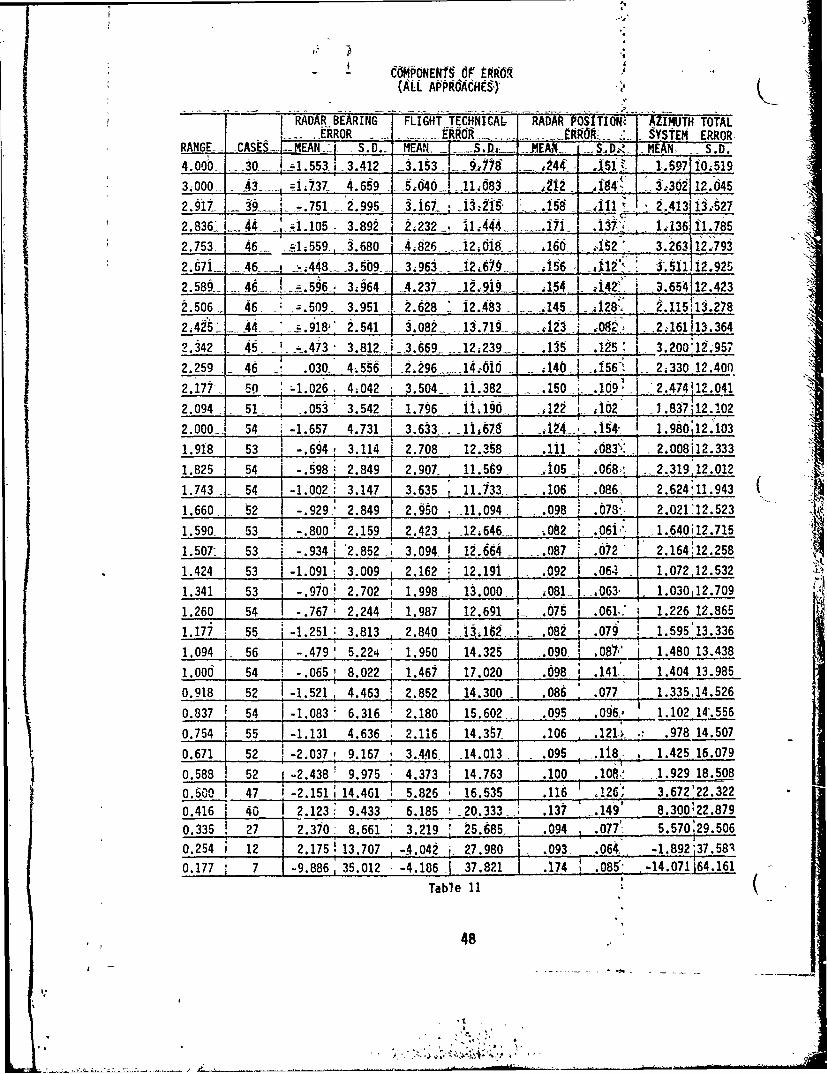
The means and standard deviations of the errors measured for all the
flights sampled are given in Table 11. The number of cases at each
range is much smaller than the corresponding number of Table 3. The
number of cases varies from 30 at 4 nm to 54 at 2 nm, in Table 11 the
latter being only one-half the maximum number of cases in Table 3. The
column labeled Total System Error represents the same variables as the
column labeled Mean Azimuth Error in Table 3. The means of Table 11
are somewhat smaller, but the difference is probably due to the smaller
sample sizes. Note that the standard deviations are quite similar.
The means of the Radar Bearing Error for all sampled flights are generally
small and negative, varying from -1.737 ° to .0530 at ranges greater than
1 nm. The standard deviations vary from 2.1590 to 5.2240 at ranges greater
than 1 nm. The mean and standard deviation change drastically at 0.177
nm becoming -9.886o and 35.0120 respectively, indicating that most of the
aircraft have begun the missed approach turn.
The Flight Technical Error means of all the sampled flights are generally
larger in absolute value than the means of the Radar Bearing Error, varying
from 1.7960 to 5.0400 at ranges more than 1 nm. The standard deviations of
the Flight Technical Error are much larger, being generally around 120 until
the missed approach turn is entered. The statistics indicate that Flight
Technical Error is the predominant component of Azimuth Total System Error.
47
wI
C0PONEN dF W6.1(ALL APPACH~) K
....... J RADAR BEARING FLIGHT TECHNICAL RADAR POSITION' AZIMUTH TOTALERROR .. ERRR ... .. RROi. SYSTEM ERROR-
RANGE, CASES..-- MEAN . S.D.- .. SIA,._ ... _E_ -_ S.D..- MEAN. S.D.
4.000 ... 30.... _ 1.553 J 3.412 -3.153 197- A M 244_-; i, 1.697 10i519
3.000 _43___1..4737 4.659 .. 4j __11,B8- --- 2 -,- 4-8 A;30 12.645
2.917 _ -75 2.995 3.16J61 .j3,21 - .166 -Alld 2.413 i3.527
2.836_ i__ 44 _14.105 . 3.892 i2 232-, i1,444 . 1. 1 1,3 .3&41.785,2.753 . 46 4.;559-, 3.680 14.826 -, _12,6 . 166 12 3.263 12.793
2.67L 46--1 _448 ...3.509.. 3.963 .1 26... _A66 12 . M 12.925
2.506 46 ";.509- 3.951 2.628 _i2_483 ,145.l 128' 2'.I1513. 8 "
2,425. - 44, 91.918 4 2.541 3.082 1j3.719_.... 123" ,, 2 -161113.364
2.342 45' _-.473 3.812.-. --3.669 ---12;239- . 15 1 3.2001.957
2.259 46 2 .030 4-.56 2;296_1 ...14,ft _ A46 156I 2z330,12.400
2.177. 50 :-1.026. 4;042 3.504_. li.3821 .150 .109,1 :2.474112.041
2.094 51 _.05D 3.542 1.76 ii,10- ,122 1.,102 1.83712.102
2.000.-. 54 . -1.657 4.731 3.633. 1i,67 ,124 , .154-- 1.980,12.103
1.918 53 -.694 3.114 2.708 12.358,. l 111 B3% 2.008i12.333
1.825 54 -.598 2.849 2.907. 11.569 .105 .068 1 2..319,12.012
1.743 54 -1.002 3.147 3.635 11.733 _-.106 .086, 2.624:11.943 t1.660 52 -.929 2.849 2.950 _11.094 .098 i .078,. 2.021,12.523
1.590 53 -. 800 i 2.159 2.423 _124646 .. 082 .06i 1.640i12.7151.507 5 3 -.934 "2.852 3.094 12.664 . 087 072 2.16412.258
____ 53 '2.852_ 3.094.___ 1 191 .09 2 2.____ _______
1.424 53 -1.091 i 3.009 2.162 12. . .092 .064 1.072,12.532
1.341 53 -.970 2.702 1.998. 13.000 ;081 . ,063. 1.030,12.709
1.260 54 -.767 2.244 1.987 12.691 .075 .061<," 1.226 12.865
1.177 55 j-1.251 3.813 2.840 13.162 . .082 .079 1.595'13.336
1.094 56 479 5.224 .950 14.325 .090 .08, 1.480 13.438
1.006 54 -. 065' 8.022 1.467 17.020 .698 141- 1.404 13.985
0.918 52 -1.521 4.463 2.852 I 14.300 .086 .077 ' 1.335,14.526
0.837 54 -1.083 6.316 2.180+ 15.602 .. .095 .0§,, 1.102 14".556
0.754 55 -1.131 4.636 v 2.116 I 14.357 .106 .12L_ .978 14.507
0.671 52 -2.037 9.167 MO3..4. .14.013. .095 _..118.- 1.425 16.079
0.588 52 -2.438 9.975 4.373 14.763 .100 .108,' . _1.929 18.508
0.500 47 -2.151 14.461 . 5.826 16.535 .116 , 3.672'22.322
0.416 j 40 2.123 9.433 6.185 _20.333_1 .137 -_.144 8.300:22.879
0.335 27 2.370 8.661 3.219 25.685, 1 .094 .077. 5.570:29.506
0.254 12 2.175; 13.707 -4.042 j- 27.980 .093_ .064, -1.892,37.581
0.177 7 -9.886, 35.012 -4.186 -1 37.821 .174 1 ,085 ,-14.071164.161
Table 11
48
'

, Table 12 represents error components of the flights which used the
p imary radar mode tracking. The means of the Azimuth Total System Error
vary from .9860 to 2.9300 at ranges greater than 1 nm. The means become
larger at the near ranges because of the missed approach turn. The
standard deviations of Total System Error are generally near 100 varying
from 9.6440 to 10.9310 at ranges greater than 1 nm. At the close ranges,
the standard deviations increase to a maximum of 46.8100 at 0.177 nm.
The Radar Bearing Error means for flights using the primary mode vary
from -1.887° to -0.0600 at ranges larger than 1 nm. The means increase
in magnitude as the ranges less than 1 nm decrease. The standard
deviations vary from 1.4240 to 4.4310 at ranges larger than 1 nm. The
largest standard deviation is 29.4160 at .177 nm.
The Flight Technical Error means for flights using the primary mode
vary from 1.8690 to 4.0220 at ranges larger than 1 nm. The corresponding
standards deviations vary from 8,2470 to 11.3840. The standard deviations
increase to 26.1870 at .254 nm.
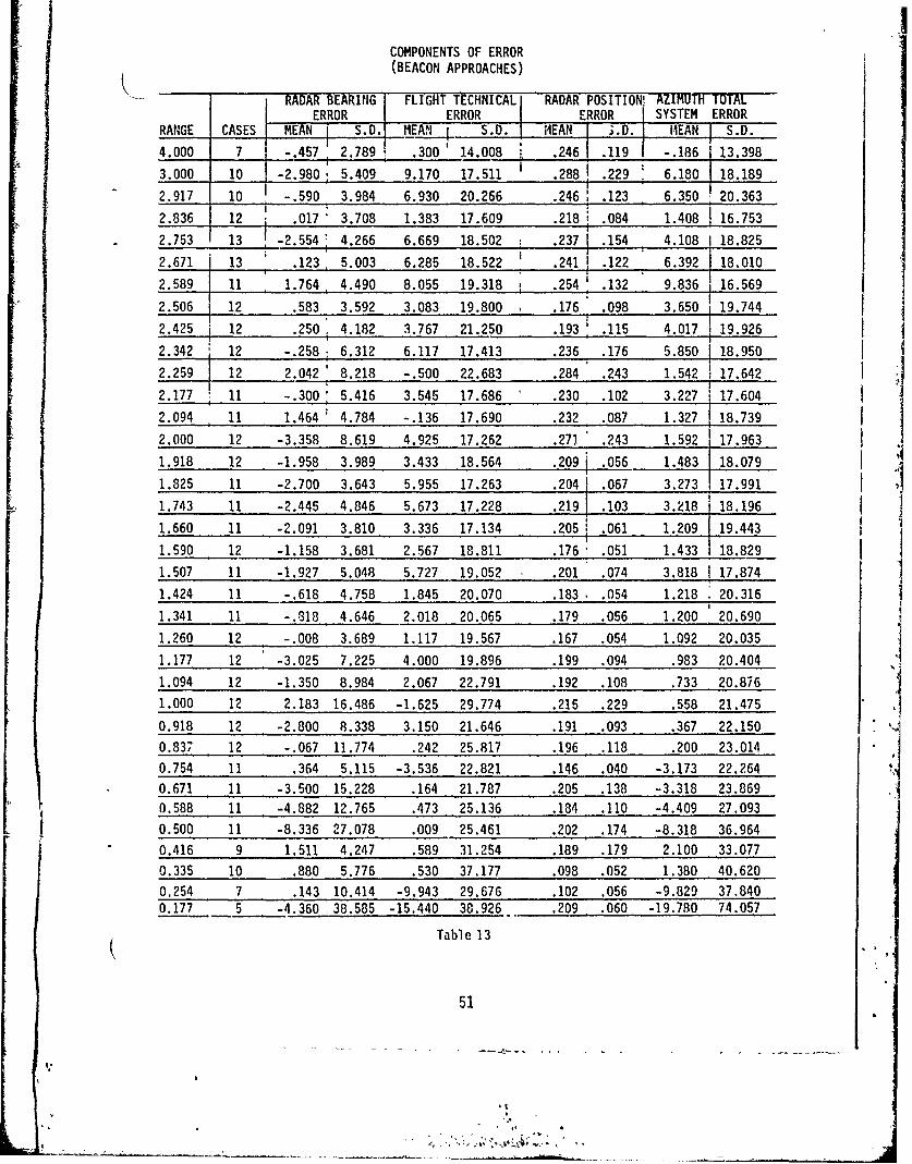
Table 13 represents components of error of the flights which used beacon
mode radar tracking. The sample sizes are very small with the largest
sample having only 13 cases. The Azimuth Total System Error means are
generally larger than their counterparts taken from the primary mode
samples.
49
I.

COMPONENTS OF ERROR(PRIMARY APPROACHES) _
RADAR BEARING FLIGHT TECHNICAL{ RADAR POSITION ; AZIMJTH TOTAL -ERROR ERROR ERROR SYSTEM ERROR
RANGE CASES MEAN S.D. MEAN S.D. MEAN I S.D. MEAN S.D.
4.000 23 -1.887 3.568 4.022 8.314 .244 .162 2.1391 9.776
3.000 33 -1.361 4.431 I 3.788 8.247 .189 i .166 2.430 9.696
2.917 29 -.807; 2.657 1 1.869 9.910 .128 .090 1.055 10.372
2.836 32 -1.525' 3.932 2.550 8.441 .154 .149 1.034' 9.644
2.753 33 -1.167, 3.414 14.100 8.553 .129 .143 2.930 9.842
2.671 33 -.673 2.782 3.048 9.713 .122 .089 2.376 10.420
2.589 35 -1.337 3.536 3.037 10.244 .122 .022 1.711 10.358
2.506 34 -.894 4.050 2.468 9.038 .135 .16 1.574 10.455
2.425 32 -1.345 1.424 2.825 10.029 .096 .044 1.466 10.247
2.342 33 -.552 2.503 2.779 9.933 .098 .076 2.236 10.189
2.259 34 -.'679 1.949 3.282 9.607 .090 .057 2.609,10.277
2.177 39 -1.231 3.627 3.492 9.206 .127 .101 2.262 10.256
2.094 40 -.335 3.082 "2.328 8.885 .092 .085 1.977 9.881
2.000 42 -1.171 2.813 I 3.264 9.783 .082 .02 2.090 10.135
1.918 41 -.324 2.759 2.495 10.176 .082 .065 2.161,0.381
1.825 43 -.060 2.372 2.128 9.741 .079 .039 2.074.10.233
1.743 43 -.633 2.494 3.114 10.084 .008 .051 i 2.472 10.0521.660 41 -.617 2.500 2.846 9.137 .069 .053 1 2.239'10.258
1.590 41 -.695 1.512 ' 2.380 10.515 .055 .027 1.700:10.613
1.507 42 -.674 1.942 2.405 10.608 .057 .028 1.731!10.570
1.424 42 -1.214 2.426 2.245 9.499 .068 .042 1.033: 9.9261.341 42 -1.010 1.996 1.993 10.777 .055 .030 .986110.022
1.260 42 -.983 1.625 2.236 10.257 .048 .029 1.264,10.308
1.177 43 -.756 1.968 2.516 10.889 .049 .027 1.765:10.931
1.094 44 -.241 3.739 1.918 11.384 .062 .055 1.684i10.922
1.000 42 -.707 2.891 2.350 11.534 .065 .081 1.645i11.350
0.918 40 -1.138 2.404 2.762 11.629 .054 .028 1.625i11.711
0.837 42 -1.374 3.740 2.733 11.594 .066 .065 1.360'11.467
0.754 44 -1.505 4.494 3.530 11.292 .096 .132 2.016 11.980
0.671 41 -1.644 6.959 4.327 11.311 .065 .093 2.698 13.392
0.588 41 -1.783 9.167 5.420 10.706 .078 .097 3.629 15.466
0.500 36 -.261 7.048 7.603 12.658 .090 .096 7.336114.336
0.416 31 2.300 10.522 7.810 16.274 .122 .139 10.100 19.335
0.335 17 3.247 10.046 . 4.800 16.954 .092 .090 8.035 21.662
0.254 5 5.020 18.348 4.220 26.187 .080 .079 9.220 38.367
0.177 , 2 -23.700 29.416 23.950 17.466 .086 086 1 .200 46.810Table 12 (
50
I.,
at a ,A ,|b l
COMPONENTS OF ERRORI(BEACON APPROACHES)
RADAR BEARING FLIGHT TECHNICAL RADAR POSITION! AZIMUTHTOTAL
ERROR ERROR ERROR SYSTEM ERRORRANGE CASES MEAN S.D. MEAN S.D. MEAN ;.D. IHEAN S.D.
4.000 7 -.457 2.789 .300' 14.008 .246 .119 -.186 13.398
3.000 10 -2.980 5.409 9.170 17.511 .288 .229 6.180 18.1892.917 10 -.590 3.984 6.930 20.266 .246: .123 6.350 20.363
2.836 12 .017 3.708 1.383 17.609 .218 .084 1.408 16.753
2.753 13 -2.554: 4.266 6.669 18.502 .237 .154 4.108 1 18.825
2.671 13 .123 5.003 6.285 18.522 .241 .122 6.392 18.010
2.589 11 1.764 4.490 8.055 19.318 a .254 .132 9.836 16.569
2.506 12 .583 3.592 3.083 19.800 .176 .098 3.650 19.744
2.425 12 .250 4.182 3.767 21.250 .193 .115 4.017 19.9262.342 12 -.258 6.312 6.117 17.413 .236 .176 5.850 18.950
2.259 12 2.042 8.218 -.500 22.683 .284 .243 1.542 17.642
2.177 11 -.300: 5.416 3.545 17.686 .230 .102 3.227 17.6042.094 11 1.464 4.784 -.136 17.690 .232 .087 1.327 18.739
2.000 12 -3.358 8.619 4.925 17.262 .271 .243 1.592 17.963
1.918 12 -1.958 3.989 3.433 18.564 .209] .056 1.483 18.079
1.825 11 -2.700 3.643 5.955 17.263 .204 .067 3.273 17.991
1.743 11 -2.445 4.846 5.673 17.228 .219] .103 3.218 18.196
1.660 11 -2.091 3.810 3.336 17.134 .205 .061 1.209 119.4431.590 12 -1.158 3.681 2.567 18.811 .176 .051 1.433 18.829
1.507 11 -1.927 5.048 5.727 19.052 .201 .074 3.818 I 17.8741.424 11 -.618 4.758 1.845 20.070 .183 .054 1.218 20.316
1.341 11 -.318 4.646 2.018 20.065 .179 .056 1.200 20.690
1.260 12 -.008 3.689 1.117 19.567 .167 .054 1.092 20.035
1.177 12 -3.025 7.225 4.000 19.896 .199 .094 .983 20.4041.094 12 -1.350 8.984 2.067 22.791 .192 .108 .733 20.8761.000 12 2.183 16.486 -1.625 29.774 .215 .229 .558 21.475
0.918 12 -2.800 8.338 3.150 21.646 .191 .093 .367 22.1500.837 12 -.067 11.774 .242 25.817 .196 .118 .200 23.014
0.754 11 .364 5.115 -3.536 22.821 .146 .040 -3.173 22.2640.671 11 -3.500 15.228 .164 21.787 .205 .138 -3.318 23.8690.588 11 -4.882 12.765 .473 25.136 .184 .110 -4.409 27.093
0.500 11 -8.336 27.078 .009 25.461 .202 .174 -8.318 36.964
0.416 9 1.511 4.247 .589 31.254 .189 .179 2.100 33.0770.335 10 .880 5.776 .530 37.177 .098 .052 1.380 40.620
0,254 7 .143 10.414 -9.943 29.676 .102 .056 -9.829 37.8400.177 5 -4.360 38.585 -15.440 38.926 .209 .060 -19.780 74.057
Table 13
51
I.j
I,!

The means vary from -0.186 o to 9.8360 at ranges larger than 1 nm and
reach a maximum magnitude at 0.177 nm of -19.780 . The standard deviations
of Azimuth Total System Error, are with one exception, much larger than
their counterparts taken from the primary mode samples. In some instances,
the standard deviations are double those from the primary mode samples.
The standard deviations vary from 13.3980 to 20.8760 at ranges greater than
1 nm. Note that 13.3980 is larger than any of the standard deviations for
the primary mode samples at ranges larger than 1 nm.
The Radar Bearing Error means for the beacon mode flights appear to be
about the same as those for the primary mode flights. The means vary
from -3.358 ° to 1.7640 for ranges larger than 1 nm. The standard deviations,
however, appear to be generally somewhat larger. The standard deviations ]vary from 2.7890 to 8.9840 for ranges larger than I nm. (
• i
The Flight Technical Error means and standard deviations for the beacon
mode flights also appear larger than those of the primary mode flights.
The means vary from -0.500o to 9.1700 at ranges larger than 1 nm while
the standard deviations vary from 14.0080 to 22.7910. The smallest,
14.008o is larger than all of the primary mode standard deviations at
ranges of 0.500 nm and larger.
The Radar Position Error means of the beacon mode flights also appear to
be larger than those of the primary mode flights. This is especially
evident since none of the beacon mode means are less than 1 nm while 23
of the primary mode means are less than 1 nm. The means for the beacon
(~52

mode vary from 0.146 nm to 0.288 nm or 877 ft. to 1,750 ft. The standard
deviations appear to be quite similar in size to those of the primary mode
flights and vary from 0.040 nm to 0.243 nm, or 243 ft. to 1,477 ft.
Since the means and standard deviations of the components of error appear
to be different for the beacon mode flights and primary mode flights,
further statistical tests were conducted. The Kolmogorov-Smirn6v two
sample test was used to compare the Flight Technical Error of the primary
mode flights to that of the beacon mode flights at the 4 nm, 3 nm, 2 nm,
and 1 nm ranges (see Appendix A). Likewise, comparisons of the Radar
Bearing Error and the Azimuth Total System Error were also conducted for
the same ranges. The null hypothesis H0 is that the samples are drawn
from the same population while the alternate hypothesis H1 is that the
samples were drawn from different populations.
The Kolmogorov-Smirnov test (Table 14) indicates that the differences
between primary and beacon radar range error samples at 4 nm, 3 nm, 2 nm,
and 1 nm were highly significant. The Radar Position Error samples at
2 nm and 1 nm were highly significant. However, the azimuth components
of error did not show significant differences except for the 3 nm Flight
Technical Error samples, but the range errors appear to be significantly
different.
The statistical analysis of the data indicates that the largest component
of azimuth error present in the final approach segment is Flight Technical
53
I

Kolmogorov - Smirnov Comparison Q_of Flight Technical Error
Probability associated with the sample
Range Primary BeaconNM Cases Cases RRE RBE RPE FTE ATSE
4 23 7 .0006* .2938 .3838 .7734 .9112
3 33 10 .0001* .7443 .0839 .0452* .5077
2 42 12 .0000* .1848 .0001* .6653 .6041
1 d2 12 .0000* .7261 0001* .6041 3329
*Significant at 5% level
Table 14
54
! i I.I
v .. -

Error. Flight Technical Error represents error introduced by the flight
crew through technique and judgment.
The analysis indicates that the error in reaching DWFAP is very large.
If the dead reckoning procedure used to enter the final approach could
be replaced with a procedure which would rely on a system such as a
highly accurate RNAV, then the dispersion of the flight paths c6uld be
significantly reduced. If a radio-navigational aid cannot be provided,
then the present procedure should be studied for possible improvements.
The procedure could be improved by a careful study of the overhead
maneuver to determine the most appropriate type of turn to use to enter
the outbound leg of the flight toward the DWFAP. A variety of turns,
such as those used for holding pattern entries, might be necessary
depending on the direction taken to enter the overhead maneuver. The
offset angle between the outbound leg and the downwind final approach
course should also be studied to determine the best angle for the airspeed
and windspeed combinations which would be expected. The amount of error
which could be eliminated by improvements in the procedure is unfortunately
unknown.
The analysis also indicates that the crews homed to the target even though
they were specifically instructed to correct their course to the downwind
final approach course. When the aircraft homes to the target, the wide
lateral dispersion at the DWFAP is maintained and other significant problems
emerge.
55
I.I

Since the final approach heading is chosen so that the approach is
directly into the wind, a large error at the DWFAP will cause the aircraft
to fly with a crosswind instead.
The homing path, under crosswind conditions, is a curve instead of a
straight line (see Appendix B). Under some rather ordinary combinations
of windspeed and crosswind angle, the curvature of such a path is large
enough that significant segments of the flight path are not visible
when using the 400 (±200) radar sweep. Since the approach procedure is
based upon using the radar for obstacle clearance during the final approach
and initial part of the missed approach, the possibility of the aircraft
flying somewhat sideways, i.e., flying a homing path under crosswind
conditions, should be minimized.
The homing tendency, together with the wide dispersion at the DWFAP,
also creates problems in the missed approach maneuver. This problem
will be discussed in the section of this paper entitled "Missed Approach
Dispersion".
An effective way to eliminate the homing curve problems would be to
provide the crew with accurate wind information with which to determine
the DWFAP and a radio navigational aid with which to accurately find it.
In addition, a device such as a cursor might be added to the radar
equipment to enable the crew to more systematically correct their course
to the final approach course. The cursor would have the added benefit
56
of enabling the crew to maintain a stable crab and hold a ground track
heading where necessary.
Another measure which may be taken to minimize the possibility of a blind
flight path due to a homing path is to simply maintain an airspeed in
excess of three times the current windspeed when using the 40 radar sweep.
As shown in Appendix B, the windspeeds which can cause a blind flight
are greater than one-third the airspeed of the helicopter. This would
also serve to minimize the possibility that a ship could move behind the
radar sweep of the aircraft and yet intersect the path of the aircraft.
This possibility is also discussed in Appendix B where it is shown that
the speeds required of the ship would be well within the operational
capabilities of many types of vessels.
Finally, the analysis shows that the largest component of error is
produced by the dead reckoning method of reaching the DWFAP. The
crewmembers do fly relatively straight, tight courses to the target
once established on a heading. Thus the lateral dispersion could be
drastically reduced by improving the method of reaching the DWFAP.
"9 57
I.t

RANGE ACCURACY
A remote handheld push button device was provided the radar controller to
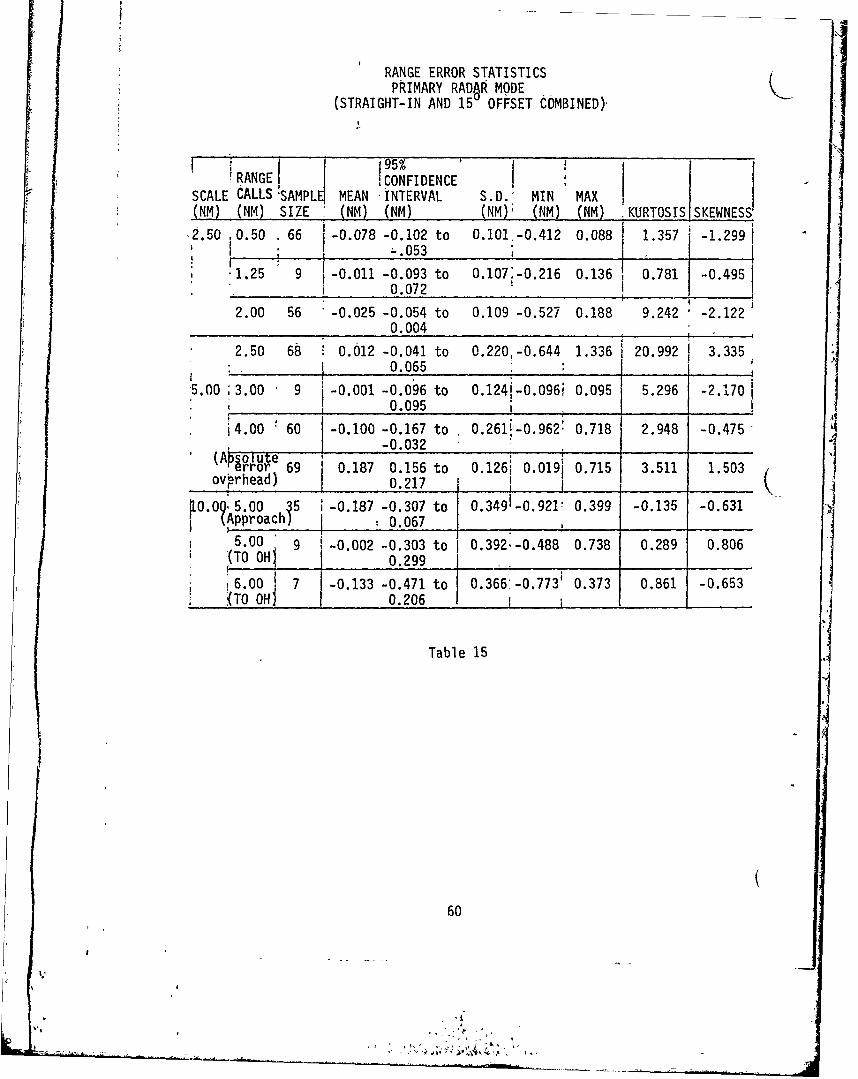
identify range "calls", specified in Tables 15 and 16. The controller
was instructed to depress the button when he determined the target was
at a given range. Depressing the button caused an event mark to be
written on the data tape at the same time as the tracker determined
aircraft position. Range Total System Error (RTSE), defined as-the
difference between controller determined range and Cubic tracker range,
was computed from the information during post flight analysis. RTSE
includes both Range Flight Technical Error (RFTE) and Radar System Error
(RSE).
Range calls for overhead, 0.25 nm, 0.50 nm, 1.25 nm, and 2.00 nm were
made with the radar range scale selector set on 2.5 nm. The range calls
made at 2.50 nm, 3.00 nm, 4.00 nm were made with the 5.00 nm range scale
selection. Range calls for 5.00 nm to overhead, 5.00 nm from target on
approach, and 6.00 nm to overhead target were made on the 10.00 nm range
scale selection. Range calls 0.50 nm, 2.00 nm, 3.00 nm, 4.00 nm, and
6.00 nm occurred on marked range rings, whereas calls at 0.25 nm, 1.25 nm,
2.50 nm, and 5.00 nm occurred between range rings requiring visual
interpolation.
The data was separated into two groups; approaches using only the primary
radar return and approaches made with the radar beacon (or transponder).
Standard statistics were computed for each group and are included in Tables
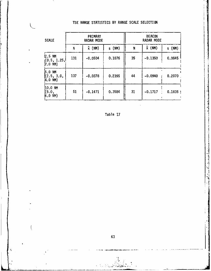
15 and 16. The data was also combined by range scale selection and the
PRECDIiG PAtX BLUdK-NOT FIMED i591
I.I
' +'-+,ii
RANGE ERROR STATISTICSPRIMARY RADAR MODE
(STRAIGHT-IN AND 15 OFFSET COMBINED),
iRANGE MA ONFIDENCE
SCALE CALLS SAMP MEAN INTERVAL .. MIN MAX(NM) (NM) SIZE (NM) (NM) (NM); (NM) (NM) IKURTOSIS SKEWNESS
9.50 !0.50 66 -0.078 -0.102 to 0.101 -0.412 0.088 1.357 1.299i:6 ' I .0j3-1-2993
725 9 9 -0.011 -0.093 to 0.107:-0.216 0.136 0.781 -0.4951i 0.072
2.00 56 -0.025 -0.054 to 0.109 -0.527 0.188 9.242 -2.1220.004 ,
* 2.50 68 0.012 -0.041 to 0.220,-0.644 1.336 20.992 I 3.335_ _ _ _ 0.065 _ _
5.00 ;3.00 9 -0.001 -0.096 to 0.124i-0.096; 0.095 5.296 -2.1701-- m ~ 0095"
;14.00 60 -0.100 -0.167 to 0.261:-0.962' 0.718 2.948 -0.475(A~s~ute-0.032ov-hed)0.217 O.6'..6
(Arjoi t _________ ___:
error 69 0.187 0.156 to 0.1261 0.0191 0.715 3.511 1.503
I0.00 5.00 35 -0.187 -0.307 to 0.3491 -0.921! 0.399 -0.135 -0.631(Approach) :0.067
5.00 9 -0.002 -0.303 to J 0.392,-0.488 0.738 0.289 0.806'(TO OHi 0.299
S6.00 1 7 -0.133 -0.471 to 0.366:-0.773' 0.373 0.861 -0.653TO OHI 0.206 1 i ....
Table 15
60
!'Iw ,

RANGE ERROR STATISTICSBEACON RADAR MODE
(STRAIGHT-IN AND 150 OFFSET COMBINED)
:95% IRANGE CONFIDENCE
SCALE CALLS SAMPLE MEAN INTERVAL S.D. MIN MAX(NM) (NM) SIZE (NM) (NM) I (NM) (NM) (NM) KURTOSIS SKEWNESS
'.2.50 0.50 13 -0.102 0.233 to 0.086 -0.233 0.0761 0.349 0.611-0.076 t I -. 3
'1.25 2 -0.193 -0.353 to 0.226 0.353 -0.0331 0 0I : -0.033 _ _
12.00 20 -0.150 -0.180 to i 0.064! 2.230 0.644o__ _ _ -0.121 " i
i2.50 20 -0.131 -0.158 to ' 0.054 -0.281 -0.0461 1.724 1-1.234-0.104 , I
.5.00 3 00 4 0.081 0.782 to 0.543-0.365 0.871; 3.080 1.642' ~~-0. 944 !
* 14.00 20 -0.092 -0.185 to 0.198 !-0.357 10.669;12.487 3.169.000
(Asolu _ e O ;errorc 12 0.1721 0.080 to 0.145 0.046 0.559 4.468 2.029overnea) 0.264;1*-- /-1IO7
!10.00 5.00 15 -0.1831-0.293 to 0.200,-0.633! 0.048: 0.278 1-1.074(Approa :h) i-0.072
5.00 3 -0.042i-0.740 to 0.281 -0.2781 0.269 0 1.123(TO OH '0.656
6.00 13 -0.189 -0.274 to 0.141 -0.375 0.059 -0.875 0.303
(TO OHb -0.104
Table 16
61
___ . ILIIl.__

statistics are presented in Table 17. A negative mean indicates that yon the average the aircraft was closer to the target than pilot and/or
radar indicated. For example, inside 2.50 nm of the target, it can be
seen from Table 16 (beacon radar mode) that the means, ranging from
-0.193 to -0.102, are negative indicating that on the average the
aircraft was 0.193 nm to 0.102 nm closer to the target than the pilot
assumed. From Table 15 (primary radar mode), it can be seen the mean
range errors ranging from -0.078 nm to -0.011 nm, were also negative.
It was not possible to identify and quantify all the causal factors of
the observed range bias.
As can be seen from Table 17, the standard deviation for primary radar
mode was approximately 0.11 nm for the 2.50 range scale selection,0.24 nm for the 5.00 nm selection, and 0.36 nm for the 10 nm range scale (
selection. Over the ranges considered, the standard deviation increased
by about 0.12 nm as the range scale was doubled. Similarly, the standard
deviation estimates for beacon radar mode ranged from 0.08 nm to 0.21 nm.
These values represent RTSE and include RSE, RFTE, screen resolution,.
and update on scan rate error.
Data was acquired which provided an estimate of the RSE component.
Discrete timed photographs of the radar screen were made, distinct from
the controller actuated photographs, and time correlated to the tracker
established aircraft position. This photographic information was digitized
and merged with aircraft position data to establish Radar Bearing Error (RBE),
62
CC
CW C ' .~
TSE RANGE STATISTICS BY RANGE SCALE SELECTION
I PRIMARY BEACONSCALE RADAR MODE RADAR MODE
N (NM) s (NM) N(NM) s(NM)
12.5 NM.5 131 -0.0504 0.1076 35 -0.1350 0.084510.5, 1.251,
2.0 NM) I II I
5.ONM_ _I NM
2.5, 3.0, 137 -0.0378 0.2395 44 -0.0940 1 0.20704.0 NM)
110.0 NM
50 51 -0.1471 0.3584 31 -0.1717 0.18351o.0NM) _ __ _ _ _
Table 17
ji2
63
77

Radar Position Erior (RPE), and Azimuth FTE (AFTE). These error quantities (
were illustrated in Figure 16. The RSE statistics are presented in Table
18 'and RBE, FTE, RPE statistics were previously presented in Tables 11, 12,
and 13. These statistics reflect the errors from the total radar system
and include such errors as radar timing and processing errors, screen
resolution, and update or scan error.
The Bendix RDR 1400 radar has been advertised to have at most a one percent
RSE with no mention of a negative range bias. Assuming the advertised one
percent value represents a two S.D. error, the one percent values have been
compared to the observed two S.D. RSE in Table 19. The comparison (Table
19) shows a much larger measured RSE than the adv,rtised one percent RSE.
However, the advertised error may not include screen resolution and/or
scan rate error. Based on the Bendix RDR 1400 CRT display matrix, radar
screen resolution is approximately 119 ft. (0.02 nm) on the 2.50 nm scale,
237 ft. (0.04 nm) on the 5.00 nm scale, and 475 ft. (0.08 nm) on the 10.00
nm scale. Assuming the screen display dot moves forward each time the
target is midway between two consecutive dots, the average screen resolution
error would be zero (no expected bias) with maximum errors of ±0.01 nm,
±0.02 nm, or ±0.04 nm for range selections of 2.50 nm, 5.00 nm, and 10.00
nm respectively.
64

K_ _RADAR SYSTEM ERROR - RANGE
PRIMARY BEACON
-. MEAN MEAN__________ ____
RAIGES CASES NM S.D. MINI MAX CASES NM MIN MAX
4.000 23___ -.062 .051 -.037 .158 7 -.185 .068___.115__.302_
3.__0 33 -.038 .060 -.042 .179 10 .161 .054 .095 .80
2.917 29 -.033 .060 1-.106 .183 10 !-.174 .064 .088 i .286t ' 4
2.836 32 -.020 .042 -.069 .103 12 -.138 .053 .063 .251
2.753 33 -.030 .082 :-.088 .353 13 -.138 .053 .063 .230
2.671 33 .032 .063 -.113 .161 13 -.131 .045 .072 .250
2.5891 35 -.024 .050-.101 .107 11 -.158 .097 .074 412
2.506 34 -.037 .051 -.075 .119 12 -.112 .053 .034 .232
2.425 32 -.031 .059 --.134 .179 12 -.128 .057 .035 241
2.342 -33 . .059 046 .231 12 -.129 .050 .061 .215
2.259 34 -.025 i .064 -.195 .171 12 -.146 .049 .075 .2412.177 39 -.036 .061 -.185 .147 11 -.141 .043 084 .213
2.094 40 -.022 * .048 -.091 .147 I 11 '-.164 .028 .122 .202
2.000 42 -.023 .039 -.066 .136 12 '-.151 .043 .095 .253
1.918 41 025 .040 j-.046 .118 12 -.152 , .038 .095 .217
1.825 43 - .013 .044 -.080 .124 11 - .147 .054 I.073 i 231
1.743 43 -.018 .044 -.081 .127 11 -.160 .066 1 .087 .333
1.660 41 -.016 .040 -.065 .093 11 -.164 .048 .115 .269
1.590 41 ".006 .041 -.081 .097 12 -.141 .048 .075 .219
1.507 42 -.002 .035 -.068 .082 11 -.156 .024 .124 .195
1.424 42 - .004 .0431 -.087 .175 11 - .143 .039 .073 .195
1.341 42 -.005 .035 -.106 .083 11 - .146 .045 .093, 244
1.260 42 -.001 .039 -.071 .127 12 - .149 .043 .082 .230
1.177 43 -.003 I .036 '-.095 .119 12 a-.135 .054 .052 .*274
1.09a 44 -.005 .041I-.068 .128 12 ,.127 .045 .038 .238 I1.000 42 -.027 .085 -.064 .518 12 - .111 .030 .055 .173 I0.918 40 - .014 .042 j-.067 .122 12 - .151 .044 .099 '.247
0.837 42 -.023 .067 -.082 .333 12 -.137 .039 .066 .218 I1 I
0.754 44 - .059 .138 '-.071 .767 11 - .129 .042 .060 .195
0.671 41 - .029 .056 -. 0.9 .290 11 i-.146 .031 .100 .191
0.588 41 - .036 .055 -.053 .203 11 I.144 .041, .084 .223
0.500 36 -. 059 1 .098 -.077 .409 I 11 I-.128 .088 ,-.072 [.298
Table 18
65

COMPARISON OF ONE PERCENT AND MEASURED RSE
RNEONE A~RCEf4T ERROR PRIMARY RSE BEACON RSE
RAG ASMD2 S.D. VALUES) 2 S.D. VALUES 2 S.D. VALUEJ(cNM) ASUE (NM) J(NM) (NM) I0.50 0.005 0.196 0.176
1.25 0.013 0.078 0.0861
2.00 0.020 0.078 0.086
2.50 0.025 0.102 0.1061
3.00 0.030 0.120 I 0.108
4.00 0.040 j 0.102 [ 0.136
Table 19
66j
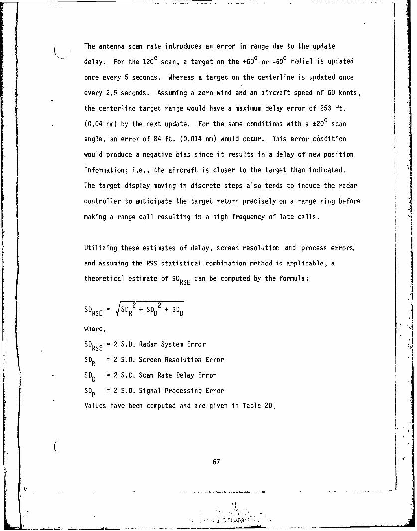
The antenna scan rate introduces an error in range due to the update
delay. For the 1200 scan, a target on the +600 or -600 radial is updated
once every 5 seconds. Whereas a target on the centerline is updated once
every 2.5 seconds. Assuming a zero wind and an aircraft speed of 60 knots,
the centerline target range would have a maximum delay error of 253 ft.
(0.04 nm) by the next update. For the same conditions with a ±200 scan
angle, an error of 84 ft. (0.014 nm) would occur. This error c6ndition
would produce a negative bias since it results in a delay of new position
information; i.e., the aircraft is closer to the target than indicated.
The target display moving in discrete steps also tends to induce the radar
controller to anticipate the target return precisely on a range ring before
making a range call resulting in a high frequency of late calls.
Utilizing these estimates of delay, screen resolution and process errors,
and assuming the RSS statistical combination method is applicable, a
theoretical estimate of SDRSE can be computed by the formula:
22SD = SD + SD + SDRSE R2 D +D
where,
SD 2 S.D. Radar System ErrorRSE
SD = 2 S.D. Screen Resolution Error
SDD = 2 S.D. Scan Rate Delay ErrorSDp :2 S.D. Signal Processing Error
Values have been computed and are given in Table 20.
(67

TWO S.D. RADAR ERROR COMPONENTS
RANGE SD SD SOp SDRsE
(A/C speed (1%) (By RSS)60 gts+60- sweep) i
0.50 .04 .08 .005 .090
1.25 .04 .08 j .013 .090
2.00 .04 .08 .020 .092
2.50 .08 .08 .025 .116
3.00 .08 .08 .030 .117
4.00 .08 .08 .040 .120
5.00 .16 .08 .050 .186
6.00 .16 .08 .060 .8
Table 20
68
'I ,
A~l
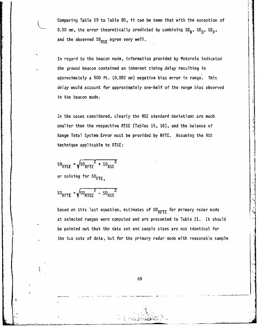
Comparing Table 19 to Table 20, it can be seen that with the exception of
0.50 nm, the error theoretically predicted by combining SDR , SDD , SDp,
and the observed SDRSE agree very well.
In regard to the beacon mode, information provided by Motorola indicated
the ground beacon contained an inherent timing delay resulting in
approximately a 500 ft. (0.082 nm) negative bias error in range. This
delay would account for approximately one-half of the range bias observed
in the beacon mode.
In the cases considered, clearly the RSE standard deviations are muchsmaller than the respective RTSE (Tables 15, 16), and the balance of
Range Total System Error must be provided by RFTE. Assuming the RSS
technique applicable to RTSE:
SDRTsE = SDRFTE + SDRsE
or solving for SDFTE,
SDRFTE = R - S
Based on this last equation, estimates of SDRFTE for primary radar mode
at selected ranges were computed and are presented in Table 21. It should
be pointed out that the data set and sample sizes are not identical for
the tt.o sets of data, but for the primary radar mode with reasonable sample
69
I.
!'
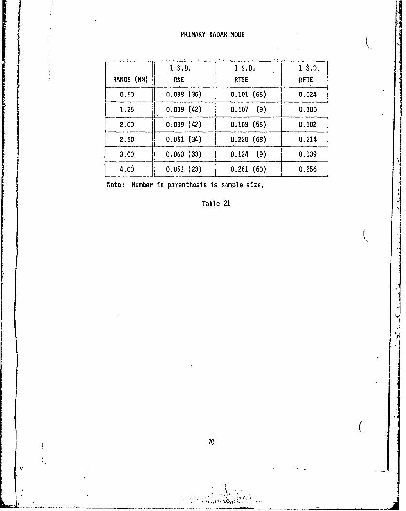
PRIMARY RADAR MODE
1 S.D. 1S.Di 1 S.D.
RANGE (NM) RSE* RTSE RFTE
0.50 0.098 (36) 0.101 (66) 0.024
1.25 0.039 (42) 0.107 (9) 0.100
2.00 0;039 (42) 0109 (56) 0.102
2.50 0.051 (34) ! 0.220 (68) 0.214
3.00 0.060 (33) 1 0.124 (9) 0.109
4.00 0.051 (23) 0.261 (60) 1 0.256
Note: Number in parenthesis is sample size.
Table 21
(
70i
II

size, a comparison of RSE, RTSE, RFTE was made. Because of the limited
sample sizes, no SDRFTE values were computed for beacon radar mode, but
a comparison of RSE and RTSE is given in Table 22. It is apparent that
RFTE is the major error component of RTSE, at all ranges except 0.5 nm.
Range accuracy plays a significant role in the selection of a Missed
Approach Point (MAP) and on the concept of using radar to provide
clearance from surface targets. Assuming a 60 kt. approach speed, 500
fpm descent rate and a 1,000 ft. altitude at the 4 nm DWFAP, an aircraft
would be at a 200 ft. MDA approximately 2.5 nm from the target. During
tracking to the target over this 2.5 nm, it would be necessary for the
aircraft to maintain lateral clearance of surface obstacles, 200 ft. AGL
or higher, by previously planning an approach course sufficiently clear
of obstacles or maneuvering around them by reference to the radar. The
radar avoidance capability is a function of such factors as system
accuracy, pilot/aircraft performance, and system limitations. The system
accuracy necessary for obstacle avoidance is a function of both range
error and bearing error. Bearing or azimuth error was discussed previously.
The combination of range and bearing error is defined to be Radar Position
Error (RPE) illustrated in Figure 16. RPE statistics at selected ranges
are given in Tables 11, 12, and 13. Essentially, RPE identifies the
radius of error associated with aircraft position established by radar
but does not include AFTE or RFTE. Figure 17 illustrates this concept.
71
,4.

BEACON RADAR MODE
RANGE RSE RTSE(NM) 1 S.D. I S.D.
0.50 0.088 (Ii) 0.086 (13)
1.25 0.043 (12) i 0.226 (2)
2.00 0.043 (12) 0.064 (20)
2.50 0.053 (12) 0.054 (20)
3.00 0.054 (10) 1 0.543 (4)
4.00 Ii 0.068 (7) 0.198 (20)
Table 22
(
f.1
72
I.i
.,. J 1
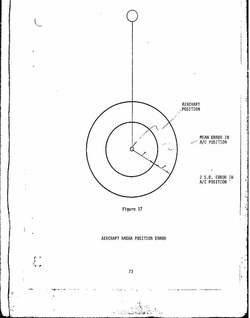
AIRCRAFT,POSITIONI
MEA ERROR I7 . ~~~-~A/C POSITION MA M:
2 S.D. ERROR IN 'A/C POSITION '
Figure 17
AIRCRAFT RADAR POSITION ERROR
73r

With reference to Tabl's 11, 12, and 13, the two S.D. circular error
varied from 0.197 nm to 0.432 nm over the ranges 2.50 nm to 0.50 nm
from the target. Exp essing the second case in terms of probability,
aircraft position established by radar was within a circle of radius
0.432 nm with center at the actual position 95 percent of the time.
Tables 15 and 16 summarize range error at the 0.5 nm Missed Approach
Point (MAP) for primary and beacon radar modes. At 0.5 nm, the mean error
is -0.078 nm with a 0.101 nm S.D. for primary and the mean error is -0.102
nm with a 0.086 nm S.D. for the beacon radar mode. The two S.D. point
(approximately 95 percent probability) of the MAP identification was 0.28
nm and 0.27 nm beyond the actual 0.5 nm MAP for primary and beacon radar
mode respectively. Stated in another way, 95 percent of the aircraft
had identified the 0.5 nm MAP within 0.22 nm and 0.23. nm of the target
for primary and beacon radar mode respectively. As can be noted from
Tables 21 and 22, Radar System Error (RSE) is the dominant error at the
0.5 nm MAP; i.e., the radar itself is responsible for most of the range
error observed at the 0.5 nm MAP. These values clearly indicate that
with the existing system, the MAP should not be 0.25 nm or less. However,
to establish MAP minimums, the pilot/aircraft performance during the
turnino missed approach maneuver must also be considered. This is
discussed in a later paragraph.
74
MISSED APPROACH DISPERSION
Prior to the statistical analysis of the missed approach segment of the
maneuver, the graph and log of each flight was carefully examined to
eliminate data which was not representative of the intended flight
operation due to either a crew blunder or an equipment malfunction. The
portion of the graph which lay between the point where the aircraft was
one mile from the target and the point where the aircraft had completed
a 900 heading change was used in the analysis.
The graph of each flight in which the crew turned to the left was
mathematically transformed so that the turn could be treated as a right i
turn. The graphs were then grouped into four categories - offset approaches
with a one-half mile missed approach point, offset approaches with a one
quarter mile missed approach point, straight-in approaches with a one-half
mile missed approach point, and straight-in approaches with a one-quarter
mile missed approach point.
Figure 18 is a composite graph of the offset approaches with a one-quarter
mile missed approach point. Four graphs were used in the analysis. Three
of the graphs ended outside the intended clear zone which is bounded by
the negative x-axis and negative y-axis. One of the graphs came within 200
feet of the target rig. Low altitude flights outside the clear zone are not
guaranteed lateral separation from surface obstacles.
Figure 19 is a composite graph of the offset approaches with a one-half mile
missed approach point. Twelve of these graphs ended outside the clear zone.
75
-. 7

r 1 II Ii'I -
I ~-~- A
* . I (j 1 I
it
~i77 ~r~--~-t---:-~- ~ - -
-4 -- ~-.~I I I
I ~I I I
- .<
liii Jill...................................I
I f.j..~ .- .~...........{...............i..........I I I *~....- I
I 'I~L2:7t7TIv L.±2±±... ~ I* I
r~~~~1~~ LL~1GM TU~NS4~ I---J
I ~t-~
....u-- I
[HOU AND FEE £- -- ..-. -I-.......Ijj.~ j ~~~!j (
'I I I . IF~gure~18 1
'1.
- 0 &-.
~ -

Nv.1
LL IGtTUONS I
hL- IFEST FIqPRO C HE F4.F.MILE. .
-. 1
I Fiur 19
Iii 11771

Two of the flights passed within 750 feet of the target rig. The
composite graph clearly shows the wide dispersion of the flights at one
nautical mile from the target. This wide dispersion is the result of
the wide dispersion at the DWFAP combined with the homing track flown
by the crew.
Note that some of the flights such as the one labeled A in the figure
would not have flown outside the clear zone if the aircraft had been on
the intended final approach path.
The arc in Figure 19 is of radius one-half nautical mile with center at
the target rig. Several of the flights initiated the missed approach
turn well within the one-half mile missed approach distance. One flight
continued about 3,900 feet after crossing the one-half mile MAP before
initiating the missed approach turn. 4
The crewmembers occasionally continued the offset portion of the flight
after radar contact with the target had been lost. The flights labeled
B and C began the missed approach turn with the target rig well behind
the aircraft.
The turns also exhibit a wide variety of turn radii. Some aircraft turned
with a radius of about 3,000 feet while others turned with a radius of
about 1,400 feet.
78

Figure 20 is a composite graph of the straight-in approaches with a one
quarter mile missed approach point. Eight graphs were used to construct
this composite graph. Seven of the graphs terminated outside the intended
clear zone, the area in the lower left quadrant bounded by the negative,
x-axis and negative y-axis. Two of the flights penetrated the cluster
region, the upper right area bounded by the positive x-axis and the
positive y-axis. The graph indicates that the quarter mile missed approach
turn is likely to be made within the cluster region.
Figure 21 is a composite graph of the straight-in approaches with a one-
half mile missed approach point. Eight of the graphs ended outside the
clear zone. One of the graphs passed within 500 feet of the target rig.
These graphs are also widely dispersed at one nautical mile from the
target. This wide dispersion is the result of the wide dispersion at the
DWFAP combined with the hoaing track flown by the crew.
Several of the flights, such as the one labeled A, would not have flown
outside the clear zone if the aircraft had been on the intended DWFAP.
The arc in Figure 21 has a radius of one-half mile with center at the
target rig. All of the graphs initiate the missed approach turn inside
the one-half mile MAP.
7979 =
I.i
\ •

LiPRCHP Q6T M I I
- -~2.
-' ~ ~ HO3N FEE" I-.4-i----~--.. Fi e' 7 2-I 0
I1 0

;L IG TL NS-
17 --1-e21

The graphs also exhibit a wide variety of turn radii. Some of the graphs
would not have ended outside the clear zone if the turn had been expedited.
The offset approaches with a one-half mile MAP and the straight-in approaches
with a one-half mile MAP were statistically analyzed. The approaches having
one-quarter mile missed approach point were not statistically analyzed due
the the small sample sizes.
The statistical analysis was accomplished by first determining circles which
best fit the apparent center of the composite graphs of each type of missed
approach maneuver. Then standard statistics were computed on the points
where the graphs cross rays emanating from the centers of the circles of
best fit (see Appendix A for a detailed explanation). The means and
standard deviations thus found were used to determine mean paths and two
standard deviation envelopes for each type of missed approach maneuver. (
The statistics for the offset approaches are found in Table 23 while the
graphical representation of the mean path with its envelope is found in
Figure 22. The means found in Table 23 represent the average distance
from the center of the best fitting circle at which the graphs cross the
rays emanating from the center. The center for the offset approaches is
located at x = 5,000 feet, y = 6,800 feet. The ray labeled 00 passes
through the center perpendicular to the x-axis while the ray labeled 900
passes through the center perpendicular to the y-axis.
82
.iI
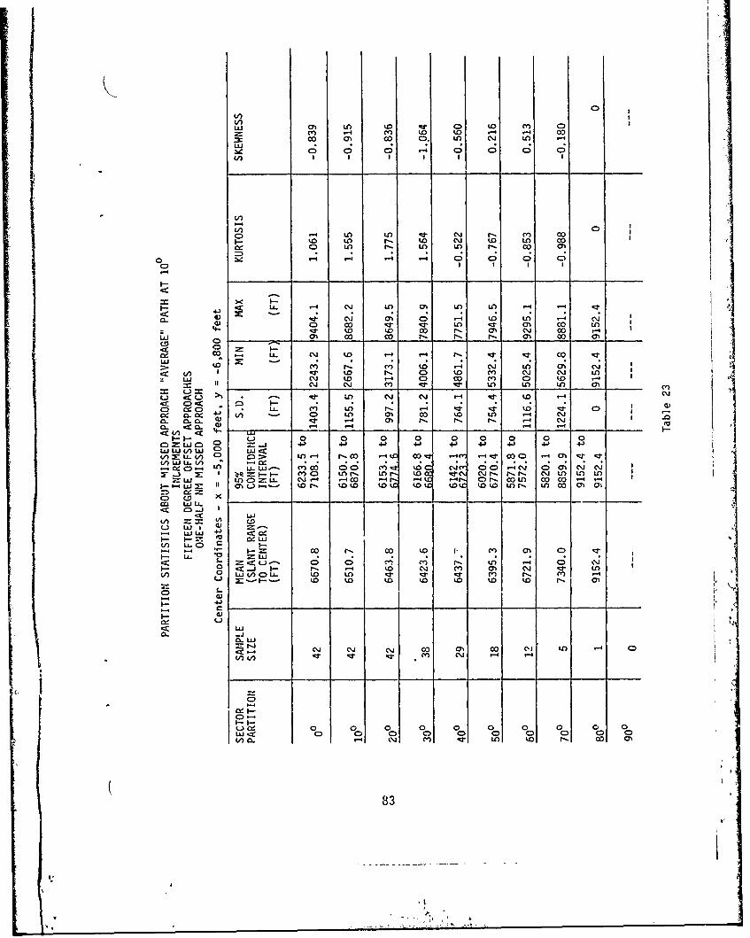
K.)C 4 CV) to %D -4 1-4 Co
C) LC) Co 0.r CM r, mn -
0 0e 0 -
w , M: - 4 c; I a;k a
o tD 0n r- M-CM a C~) 00I- 10 CC) 0-- 1 r a0 CYI0In C
0o LL. le. 10 In 1:r 0o -s x- -4 -
ol r- Ce to -4Ij) O \
01c to fl In to m '~ Coj In
I- '4j CM -4 C) co mn C4 t.0 1
a.W 4 ;C U') 01 co %0 LO CM i CO0L -- 4 -)- l
00 0 0- C' 0 M In 0' 0m u 10 CD 0j 40 4) 4) +M In 4W Wu in w0 0l Co C 0
V) CM C'. Ln Ln In OfI 0
Lt- W ~ c; In C3 CM m- ko 10 oo - -4Da c= 0 I- (Y a Inr nr o w l . r ~ n t)Lo - Ou 0 LOC LL. C')1 -4C In I f- 14 C) O LO Co- 00 i- 4 0
I-- - 0 In 0) C, k o ok o to ID% n -4 CM o a) (r
~C) C tLa W 0
o C.D X
LL) Li.
-:C- LLJI- =~ 40 C0 0 t . YJC
I-- L.0 = Wcc -Ur- Co C-.4 c~- u . 0 < i ( N J m 00 ~ ') * 0~ 0z U l
Ln 0 L (A C~pOLL. k0 In -13" -d' N- r ()
C>I-
cCW
Cd u~ 1' CM -4
C- wL 0-j
0: "0~ ~ ~ 0 0 0N 00 0l 0 0
0 0 0 0 0 0 0 0 0V)0 CL-4 CM cv) -cq In) to f- co m'
83

L-1
M:L L) uC cLUM'(. C17 ZQ.IU) D Q/. C!) c
.- J-U-)LUJ MfLLJ
I :: z I >
~ LU LU
I.--
~i
z -
P 4-

CE LU L) CE iLJz -. CCX D-.
I > I _---
EDZ ~ED
-~
0C:
C)
0' S-1 0,0S-01'IW''NQI.HI]O \OHK GO)85I

The graph of the meanpath of the offset approaches with the two standard (
deviation envelope (Figure 22) is oriented differently due to the 150
offset path taken at I nm. The MAP is located to the right of the target
rig. The envelope is 4,456 feet wide at the MAP and narrows to 3,017
feet at the 50 radial. The envelope then widens considerably, but
sample sizes of the remaining radials are much smaller. The reduction
in sample size is due to the fact that most of the aircraft have completed
a 900 heading change.
The mean path of the offset approaches is 2,066 feet from the target at
its closest point while the two standard deviation envelope is 506 feet
away at nearest point from the target. The mean path and its envelope
extend outside the clear zone, but the samples sizes for the portion of
the path outside the clear zone are small. The sample sizes are adequate
at the 400 radial to support the proximity of the mean path and 95 percent
envelope to the target.
If the missed approach distance had been three-quarters mile instead of
one-half mile and if the flight crews flew with the same proficiency, then
the y-axis could be moved one-quarter mile to the left to the position of
the dashed line of Figure 22. The target rig would then be located at
the intersection of the x-axis and the dashed line. The mean path would
then be no closer than 0.5 nm-of the target rig while the envelope would
be no closer than 1,500 feet. The mean path still extends beyond the clear
zone, but it does so at a radial with a sample size of only one.
86
l4

The statistics for a straight-in approach are found in Table 24 while the
graphical representation of the mean path with its envelope is found in
Figure 23. The means found in Table 24 represent the average distance
from the center of the best fitting circle at which the graphs cross rays
emanating from the center. The center of the best fitting circle of the
straight-in approaches is located at x = -2,500 feet, y = -2,000 feet.0
The ray labeled 0 passes through the center perpendicular to the x-axis
while the ray labeled 900 passes through the center perpendicular to the
y-axis.
The graph of the mean path of the straight-in approaches with the two
standard deviation envelope (Figure 23) is oriented the same as the mean
path graph of the offset approaches (Figure 22). The missed approach
point is located to the right of the target rig with thi direction of
flight being to the left and then upward as the aircraft completes the
right turn. The envelope is 3,380 feet wide at the 00 radial and narrows
01to 1,660 feet at the 40 radial. The envelope then widens to 3,344 feet
at the 900 radial. The sample sizes decline after the 400 radial,
decreasing from 31 to 19 sample points. .
The mean path of the straight-in approaches is 1,316 feet from the target Iat its closest point while the two standard deviation envelope is 409
feet away at its nearest point from the target. The mean path stays
within the clear zone throught the maneuver, but the two standard
deviation envelope does leave the clear zone. J87

V)V)
LO C7% fq-. -- r4 U):x 04 Ai to ) Cl) 00 N. -** U -4
1.1 N. OD to - to LO ce) C4N
V) 0; 0; 0; 0; 0 0 0 0
V)
ui
U ) L O Nl W N0 0 0
00 0 0 Ci 1Nd2 Cl CD -4 CD 021 1
o 4T . .. *
0 < I- 0 C) LA to -4A C L 'L . _ _ _ _ _r _ _ _ _ r_ __4J qt O 0 0
LL l 4 r a% 1--
:2. LLJ w -4
LCA 0 0> N. -4 1-4 02 1-4 N. r,
CLJ 0L D LL. A () L . LA 0 %0 r- to Lr to to t0CL - D K) Kr N c 1-4 02 %D Cl) 1.0 cnc LA 00 LA LA T r R LA* -w to co -
0D N W~ L 0 0 0 0 0 0 0 0 0 0
(n =0% I CDJ CDv- COA CA 0o 00 m - -002 c (M0 N j NLA
V; x '-".6ff 1 61; %. 1 ; - UU) ~ ~ L LLJ c C4 Ni LAr C4) _-40 a; r -N 0L) AA N) 0
I-W bZIR - F I r- wr . n 04 U' Lr, M -V -40 co M00 -4 Cr) NNjcl LALAD=Dx Ln OZ=LL c -W~ 00C m 2. N.o ". N.O CDI*-' -4 00C' m M t 002LACU MU"J-4- v-" yli -4N C4 4 N~ 1 v-IN v-N 14N vl-IN v- ci v-IN - IN
C, 4)
<JO C D
1 0
cc -jC. ) CY) LA a% 0~ 0 i0 . N. N~LLJ r-4
4J tn C) - CD) m- 0 0 LA ) NM Nl
0 U.
-j
0 1-4 M - y-4 v-4 1I (n r- m' v-I 0)iC?) C') C') c') m' Nl N M..
1- 0-0 0 0 0 0 00 IC NC C) (D LA 0 0
88
If the missed approach distance had been three-quarters mile insteadKof one-half mile and if the flight crews flew with the same proficiency,
the y-axis could be moved one-quarter mile to the left to the position
of the dashed line in Figure 23. The target rig would then be located
at the intersection of the x-axis and the dashed line. The mean path
would then be within 2,090 feet of the target rig while the two standard
deviation envelope would be within 1,275 feet of the target rig. Both
the mean path and the two standard deviation envelope would remain
within the clear zone.
In summary, the dispersion of the offset approaches is wider than the
dispersion of the straight-in approaches. The mean path of the
straight-in approaches stays within the clear zone while the mean path
of the offset approaches does not. The envelopes of both types of
approaches depart from the clear zone. The mean path and envelope of
the straight-in approaches come nearer to the target rig than the
corresponding curves of the offset approaches. If the missed approach
distance were increased to three-que.rters mile, then the mean path
and envelope of the straight-in approaches would remain within the
clear zones.
89
I-* - - . - - - - - ~- - - - - - - - - - - - - - - -

rIOPERATIONAL DIFFICULTIES (During the course of the test, some difficulties arose which could
not bequantified and included in the statistical analysis. These
difficulties are important and step- should be taken to minimize their
occurrence.
It was found that the identification of the desired target from a group
of targets is very difficult when using the primary mode and not
completely certain when using the beacon mode. In the statistical
analysis, it appears that the tracking is possibly better using the
primary mode, but the beacon mode is desirable for identification purposes
This problem is easily understood when using the primary mode since the
helicopter is often approaching the cluster of rigs from a direction (
other than the one based on the preplanned DWFAP. In addition, the
radar presents a view of the cluster from an oblique angle rather than
from straight above as on the approach plate. The radar also presents the
targets on the screen as rather long, indistinct images which are
indistinguishable from one another and from ships operating in the area.
The crewmembers incorrectly identified the target 19 times during the test.
The overhead approach was made to a correct target, but the final approach
was to an incorrect target, 8*times. The overhead approach was made to an
incorrect target, but the final approach was made to the correct target, 6
times. The overhead approach was made to the correct target, but the final
approach was made to a ship, 5 times. This means that the crew incorrectly
90
----.

k identified the target almost 16 percent of the time and even homed on
ships 4 percent of the time. These incorrect identifications all
occurred when the primary mode was in use; however, on one occasion
the crew was forced to switch from beacon mode to primary mode, due
to equipment malfunction, during the approach and then incorrectly
identified the target.
The incorrect identification of the target could lead to an undesirable
situation when approaching a cluster of rigs, especially if a missed
approach turn is necessary.
The missed approach turn is a blind maneuver and an incorrect identifica-
tion may position the aircraft at the missed approach point such that
a turn might be made into an area which is not necessarily clear of
obstacles. Figure 24 is a graph of a flight in which an incorrect
identification resulted in a turn toward an obstacle. The approach was
planned to rig r but was actually conducted to rig 6.
,1Even during the final approach, an incorrict identification coupled with
a crosswind could cause a blind flight into an area with obstacles (see
Appendix B). ,4
The beacon mode eliminated the identification problem but created some
additional problems. Both the radar and the surface based beacon mai-
functioned occasionally. The surface based beacon was intended for use
91
V.

i.l
00,,
samw__ riou* x
920

at long distance and occasionally at close range, it caused the return
image on the radar screen to break up creating tracking difficulties.
During six of the flights, the crew reported that the beacon image was
breaking up. Before two other flights, the beacon equipment failed
completely which caused the flight to be conducted in primary mode,
During one flight, the crew was forced to switch from beacon mode to
primary mode while on the final approach. Thus, problems with the
beacon occurred during at least nine flights from a total number of
only thirty flights or 30 percent of the time while conducting approaches
in the beacon mode. In addition, the use of the beacon does not permit
a radar return of surface obstacles that must be avoided during the final
approach. Hence, the radar "see-and-avoid" concept would not be
applicable.
The crewmembers turned the wrong direction seven times during the outbound
procedure turn. This resulted in a large deviation from the DWFAP. The
large deviation from the DWFAP and the tendency to home caused the aircraft
to track toward the target along a path different from the final approach
path and resulted in a missed approach track different from the one planned.
Occasionally the target disappeared from the screen or, in the case of the
beacon mode, broke up near the missed approach point. This may have been
caused by an insufficient adjustment of the tilt angle for the horizontal
distances involved. The crew sometimes delayed the missed approach turn
when this happened allowing the helicopter to approach the rig closer than
(93
I.i
I'

the planned minimum range. This delay usually resulted from the-crew
attempt to reestablish contact with the target. This problem occurred
at least twice.
(94
1 ,
.1T

CONCLUSIONS
APPROACH TRACKING ACCURACY
1. The final approach flight track dispersions can be described by
normal distributions. The 95 percent approach envelope is funnel shaped,
about 4 nm wide at the DWFAP narrowing to approximately 1 nm at 1 nm
from the target.
2. A significant portion of the final approach azimuth error was introduced
at the DIFAP by the dead reckoning procedure and retained throughout the
approach by the tendency to home to the target.
3. Once established on target, tracking was accomplished with a reasonably
small lateral dispersion and little effort was made to regain the
intended final approach course.
4. The mean final approach path contained approximately a 50 positive bias
error, introduced most likely by the inaccuracies of the outbound procedure
and the direction of turn onto the outbound leg.
5. The largest component of azimuth error was Flight Technical Error.
6. Homing tracking flown under some crosswind conditions can produce a
curved ground track with segments not visible by the radar set on the ±200
sweep.
95

7. The current radar system does not provide a reasonable procedure to
establish and maintain a crosswind crab.
RANGE
1. A negative bias (closer to the target than assumed) was present in
both primary and beacon mode range determinations.
2. The beacon mode negative bias tended to be larger than the primary
mode for ranges inside 5 nm.
3. The standard deviation for primary radar mode was 0.11 nm for 2.50
nm scale, 0.24 nm for 5.00 nm scale, and 0.36 nm for 10.00 nm scale. The
standard deviation increased by approximately 0.12 nm as the range scale
was doubled.
4. The observed Radar System Error (RSE) was approximately the same as that
predicted by combining the advertised 1 percent error (assumed to be
processing error), delay or scan rate error, and screen resolution error
at all ranges except 0.50 nm.
5. Approximately 50 percent of the negative bias error observed in the
beacon mode was due to a timing delay present in the design of the ground
beacon used in the test.
96
U.. . ..
_____________________ *2__ _ _ _ _ _ _ _

6. With the exception of the 0.50 nm range, Range Flight Technical Error
(RFTE) is the dominant source of range error.
7. The radius of the 95 percent Circular Error Probability (CEP) varied
from 0.197 nm to 0.432 nm over the ranges 0.50 nm to 2.50 nm.
8. The Radar System Error was the dominant source of error at the 0.50 nm
Missed Approach Point (MAP).
9. The 95 percent point for the 0.50 MAP was 0.22 nm and 0.23 nm from the
target rig for primary and beacon mode respectively.
MISSED APPROACH
1. Based on the dispersion of missed approach tracks, the one-fourth
mile Missed Approach Point (MAP) is unacceptable.
2. The missed approach mean track of the straight-in approaches is closer
to the target rig than the mean track of the offset approaches.
3. The missed approach dispersion of the offset approaches is greater than
the dispersion of the straight-in approaches.
'I4. A greater proportion of the missed approaches initiated by aircraft from
offset approaches completed their turn outside the intended clear zone than
those initiated from a straight-in approach. (Aircraft must complete their
917
.;S.
. r. =
~ ,-.

missed-approach turn inside the clear zone to be guaranteed lateral
obstacle clearance.) K-
5. The point on the 95 percent envelope nearest the approach target for
the offset approach is only 97 feet greater than that for the straight-in
approach. That is, the minimum distance from the offset 95 percent
envelope (506 ft.) is not substantially greater than that of the straight-in
approach (409 ft.).
6. The missed approach dispersion is primarily due to MAP range accuracy,
performance in execution of the turn, and the large crosstrack dispersion
at the MAP. The most significant factor appears to be the large crosstrack
dispersion at the MAP.
7. If the MAP was three-fourths mile from the target, the mean path and
95 percent envelopc of the straight-in approaches would remain within the
clear zone.
GENERAL CONCLUSIONS
1. Crew coordination is critical; well developed training procedure should
be developed to prepare the crew for this task. %
2. Difference in instruments such as the directional gyro can produce
confusion. For example, if the controller and pilot DGs differ significantly,
commands such as "steer 1751 ' are inappropriate.
98

3. In using the radar in primary mode to avoid obstacles:
a. Forty degrees is unacceptable for peripherial information.
b. One hundred twenty degrees is acceptable for peripheral
information, but update and target resolution is a problem.
c. Assuming a homing technique, certain crosswind/airspeed
combinations can produce conditions in which the ground track
traverses a region not presented on radar. This condition can only
occur if windspeed/airspeed > sin [sweep angle] ; the blind
condition is most likely to occur when homing atlow airspeed on
400 sweep.
d. Manual tilt and gain controls caused some difficulties; inadvertent
or improper adjustments can result in lost target or significant changes
in target illumination.
e. The present radar system displays do not give a sufficient indication
of the magnitude of lateral separation between the aircraft and a surface
obstacle.
f. Considerable variability exists on establishing target position,
such as referencing centerline of near edge, centerline or leading
edge.
(.
99
Ad

g. Large delays are inherent in interpretation, announcement, and
pilot action.
h. The workload (tilt, gain, interpretation, announcement, etc.) is
very high when the aircraft is close in to a cluster of targets. A
busy "dynamic" obstacle environment enhances the problem. Single
platform approaches with low density dynamic obstacle environment
produce a relatively low workload.
10
(II0I
VI

-- - -_ _ _ _ i_______
RECCMMENDATIONS
APPROACH TRACKING ACCURACY
1. Where sufficiently accurate RNAV systems are available, the DWFAP
should be identified as a positive fix. To achieve improvement over the
present DR/RADAR method, the 95 percent error must be substantially less
than ±2 nm at the 4 nm DWFAP.
2. If the DWFAP can't be established by a positive fix, the DR/RADAR
procedure should be investigated for improvements.
3. The present radar system should be modified to provide a more positive
means to intercept and maintain a chosen ground track.
4. The present radar system should be modified to provide a more positive
means of maintaining a ground track under crosswind conditions.
RANGE
1. The current radar systems should be investigated to determine methods
for eliminating negative range bias.
t .12. Ground beacons with known design timing delays should not be used in
Airborne Radar Approaches.
3. Investigations should be carried out with existing radar range displays
to determine methods for reducing Range FTE.
101
C,' \
1: + -. ., ,
4. Due to range error, the Missed Approach Point should not be less
than 0.50 nm.
5. Due to the combinations of azimuth and range error, the radar should
not be used to provide lateral clearance of surface obstacles within 0.5
nm or less.
MISSED APPROACH
1. To increase the probability of remaining in the missed approach
clear zone, the straight-in approach should be used during approaches
to clusters.
2. To reduce the missed approach dispersion, the accuracy of acquiring
the DWFAP should be improved and homing tracking should not be used.
3. To increase probability of lateral clearance of cluster and/or target,
the crew should be trained to expedite the missed approach turn.
4. The crew should be trained to immediately initiate a missed approach
when the radar target is lost.
5. The range system accuracy (crew and radar) for establishing the MAP
range should be improved.
6. The crew should be trained to initiate the minimum radius missed
approach turn deemed acceptable for IFR maneuvering in the aircraft used.
102
( -
K GENERAL RECOMMENDATIONS
1. This type approach requires high crew coordination; all flight crews
making this type approach should be provided extensive training before
approaches under actual instrument conditions are made.
2. Instruments frequently referenced by controller and pilot should be
closely calibrated to each other and anY differences clearly noted by
the crew, e.g., directional gyro.
3. If the radar is used for obrtacle avoidance, it should be set in primary
mode or a combination primary/beacon mode, with 1200 sweep, and the aircraft
should not "home" to the target, and the approach should not be flown under
conditions where
windspeed/airspeed > sin [sweeP angle ]
4. The radar display should be modified to improve ground tracking reference,
holding a crab, indication of lateral clearance, target identification.
5. If technically and economically feasible, it would be desirable to have
a system that would "lock" on the target, thus substantially reducing
controller workload.
103

Appendix A
COLLECTION OF DATA - FINAL APPROACH'
During each helicopter flight, the position of the helicopter relative to
the target was computed at one second intervals. The position of the
aircraft was recorded in cartesian coordinates with the origin set at
the target, the positive x-axis in the direction of true north, the
positive y-axis in the direction of true east, and the positive z-axis
upward. In addition to the position, the horizontal distance from the
aircraft to the target as well as several other variables such as aircraft
heading and airspeed were recorded each second. Since the approach was
to be made into the wind, the wind direction (the intended approach
heading) for each flight was recorded.
EXTRACTION OF DATA - FIMAL APPROACH
In order to analyze the lateral, did vertical dispersion of the flights
on the downwind final approach, the position, range from target, ground-
speed, ground heading, airspeed, and aircraft heading of each aircraft
when at 5 nm from the target on final approach was recorded to form one
sample. In a similar manner, the position and the other data described
above, for each aircraft, was recorded when the aircraft reached 4 nm,
3 nm, and then in decreasing 500 foot intervals to the missed approach
point for the particular flight, to form 35 other samples. Each sample
contains the data from all the flights at a particular distance from the
target rig. The samples vary in number of cases since not all flights
reached a distance of 5 nm from the target and occasionally, due to
I10 FF.EC~fJ%G PAGE BLjdjZx..IT i' z I n

technical difficulties at the time of a flight, data at a particular
range was missing.
LATERAL DISPERSION STATISTICS - INTENDED-COURSE
The lateral dispersion statistics were computed on each sample by finding
the angle formed by the intended approach course line and the line
joining the aircraft position and the target rig. This was done by first
finding the perpendicular distance D from the aircraft position to the
intended course line. The distance was recorded as positive if the
aircraft was located on the right side of the intended course looking
toward the target, and negative if the aircraft was located on the left
side of the intended course. The angle A was then computed by the formula
A = Arcsin (D/R) where R is the distince to the target.
INTENDED COURSE
A TARGET
DR
AIRCRAFT
Figure A-1
Standard statistics of this angle such as the mean, variance, skewness,
and kurtosis were computed for each sample on all flights, the offset
106
I,
I." ,

flights, and the straight-in flights. These statistics may be found in
Tables 3, 4, and 5. Graphs of the mean paths with two-standard-deviation
envelopes may be found in Figures 10, 11, and 12.
The sample sizes of the experiment are small, so in order to fit probability
density curves to the lateral dispersion data with high confidence, larger
samples are required. A large sample may be formed by combining smaller
samples when the samples are statistically from the same population and
the samples were formed independently.
The lateral position of the aircraft at a particular distance is given in
terms of the angle of displacement. Inspection of the standard statistics
of this angle for the various samples indicate that the samples may
possbily be considered to come from the same population although no
statistical tests were performed to support this conclusion. Inspection
of the data also indicates that the aircraft lateral position in one
sample may be correlated to its lateral position in another. To test
for correlation between samples, the Spearman rank correlation test was
employed.
The Spearman rank correlation test was performed for each pair of adjacent
samples and for each pair of samples located at half-mile intervals (Tables
6 and 7). The test indicates that the null hypothesis should be rejected
in every case. Therefore, the samples of lateral deviation were not
combined.
107
- *' V

Although sample sizes are small, each sample was analyzed to determine Qif the samples could be considered to be from normal populations. If
samples are drawn from a population then the sample kurtosis and skewness
are random variables. The distributions of the skewness and kurtosis of
samples drawn from a normal population are known (reference 1).
If a sample is drawn from a normal population then it would be unlikely
that the absolute value of either the skewness or kurtosis would be large.
Thus the null hypothesis H is that the sample is drawn from a normal0
population and the alternate hypothesis HI is that the sample was drawnfrom a population which was not normal. From tables of critical values
of skewness and kurtosis, it was determined that the null hypothesis could
not be rejected for any of the samples.
LATERAL DISPERSION STATISTICS - AVERAGE COURSE
The lateral dispersion statistics described above are indications of the
dispersion from the intended course given by the wind direction. These
statistics do not measure how well the pilot homed to the target rig,
but instead measure how well the pilot followed the intended course. In
order to measure lateral dispersion independently of the intended course,
the average course for each flight was computed and then statistics of
dispersion from these average courses were computed. The average course
for a flight was computed while the data for the intended course was being
extracted. The average Aof the angles of the dispersion corresponding to
4 nm through 1 nm was found for the flight. Then A was subtracted from
the intended course heading to establish the average course.
108
I.
A - ' ,

Using the same sample points, the lateral dispersion angle formed by
the average approach course line and the line joining the aircraft
position to the target rig was found. The perpendicular distance D
from the aircraft position to the average course line was found. The
angle A was then computed by the formulaa
A = Arcsin (D/R)a
where R is the distance to the target.
INTENDED COURSE
AVERAGE COURSE / o TARGE
f/7D iAIRCRAFT
Figure A-2
Standard statistics of this angle were computed for each sample on all
flights, the sample points from the offset flights, and for the sample
points from the straight-in flights. These statisiics may be found in
Tables 8, 9, and 10. Graphs of the means with two-standard-deviation
envelopes may be found in Figures 13, 14, and 15.
(109
I.
- S
EXTRACTION OF DATA-MISSED APPROACH
The missed approach segment of the flight presented very special problems
in data extraction and analyzation. Two maneuvers were used in the
experiment; a circular turn either left or right initiated at the missed
approach point, and a 15 degree heading change, called an offset, at
1 nm followed by a circular turn initiated at the missed approach point.
The pilot was allowed to choose the direction of the turn, depending on
the location of obstacles in the vicinity, thus creating a mixture of
left and right turns.
The coordinate system for each individual flight was rotated until the
negative y-axis coincided with the intended final approach line, the
positive x-axis then pointed to the left of the intended course giving
a left hand coordinate system. Then the sign of each x-coordinate of
each left turn was changed so that a right turn, the mirror image of the
original left turn, was created. This procedure made all turns into right
turns and permitted composite graphs of the circular turns and the
offset turns to be made (Figures 6, 7, 8, and 9).
From the graphs, circles were determined which best fit the center of
the area covered by the turns. Then, to find the average path flown
precisely, the position of each flight as it crossed 100 radials
emanating from the center of the best fitting circle was found. (See
Figure A-3.)
(11i PRECEDi.G B"a-NOT M-FPIUD
...I'
122
JI
•, -

MISSED APPROACH DISPERSION STATISTICS KBASED ON SECTOR PARTITIONS ALONG "AVERAGE" PATH
0I
900
20 0 N
10 n
0 0
Figure A-3
112(
-- - - - -- - - - -

LATERAL DISPERSION - MISSED APPROACH
This procedure produced 10 samples for the circular turns and 10 samples
for the offset turns, each sample being a slice along a 100 radial of the
flight paths. Within each sample the distance of each point from the
center was found and standard statistics for the distance were computed.
These statistics may be found in Tables 23 and 24. The average distances
together with two-standard-deviation upper and lower bounds were plotted
on their corresponding radials to produce graphs (Figures 22 and 23) of
the average paths with two-standard-deviation envelopes.
DATA COLLECTION - RANGE INTERPRETATION ERROR
The crewmembers of the helicopters were provided with a contact switch
so that they could place a mark on the data tape of the flight. The crew
was requested to mark the data when, from observation of the radar screen,
they determined that the aircraft was at specified distances or ranges
from the target. (The test was designed to detect differences in the
ability of the crew to determine distances when using the primary mode
as opposed to the beacon mode. It was also designed to detect differences
in determining distances between scales and to detect differences between
offline distances and online distances.) . :1
1i
113
S I - _______________________

STATISTICAL ANALYSIS - RANGE INTERPRETATION ERROR
The data collected represents the true range of the aircraft from the
target when the crew indicated the range of the aircraft. In order to/ detect differences, the data was arranged into two matrices with the
rows of each being data collected from the individual flights. The first
matrix was from aircraft operating in the primary mode and the other matrix
was from aircraft operating in the beacon mode. The columns contained
the true distances for each specified distance. That is, the first
column contained the true distance when the crew endeavored to mark 1/4
nm, the second contained the true distance when the crew attempted to mark
1/2 nm. The true or specified'distance was subtracted from the entries
of each column. For example, 1/4 nm was subtracted from each entry of the
first column and 1/2 nm was subtracted from each entry of the second column.
Standard statistics were computed for each column of each matrix. The Mann- (Whitney U test was used to test corresponding columns of the two matrices
for differences and the Kruskal-Wallis test was used to test for differences
between columns within each matrix.
DATA COLLECTION - FLIGHT TECHNICAL ERROR
A camera was focused upon the radar screen and photographs of the display
were made at regular intervals during the final approach segment of each
flight. The photographs were made most frequently during the final approach
segment of each flight. Camera malfunctions caused the number of flights
sampled in this manner to be smaller than the number of flights actually
flown.
114
• .

( The position of the helicopter, as indicated iy the radar, was accurately
determined from each photograph and compared to the actual position of
the aircraft at the time the photograph was made. This resulted in values
of the Range RSE, Radar Bearing Error, Radar Postion Error, and Azimuth
Flight Technical Error corresponding to each photograph.
DATA EXTRACTION - FLIGHT TECHNICAL ERROR
In order to analyze the data, the Radar Range Error, Radar Bearing Error,
Radar Position Error, and Angular Flight Technical Error of each aircraft
when at 4 nm from the target on final approach was recorded to form one
sample. In a similar manner, the data described above for each aircraft,
was recorded when the aircraft reached 3 nm and then in decreasing 500
foot intervals to the missed approach point for the particular flight
to form 33 other samples. Each sample contains all the available data
from all the flights at a particular distance from the target rig.
STATISTICAL ANALYSIS - FLIGHT TECHNICAL ERROR
Standard statistics of each type of error were computed for each sample
on all flights, the flights using the beacon mode, and the flights using
the primary mode. The statistics may be found in Tables 15, 16, and 18.
The Kolmogorov-Smirnov two sample test was used to compare the Range RSE
data from the flights using the beacon mode to that of the flights using
the primary mode from the 4 nm, 3 nm, 2 nm, and 1 nm samples. Similarly,
the other types of error were tested to determine possible differences
115
A1. I

-between the data taken from the flights using the beacon mode and the
flights using the primary mode. The results of these tests may be found
in Table
MANN-WHITNEY U TEST
The Mann Whitney U test is used to test whether two independent groups
have been drawn from the same population. It is one of the most powerful
nonparametric tests, and it does not require the assumptions necessary
for the parametric t test.
Given a sample A and a sample B, let the null hypothesis H0 be that A and
B were drawn from the same population and let the alternate hypothesis H1
be that the population from which A was drawn is stochastically larger
than the population from which B was drawn. Let NI be the number of cases
in the smaller of the two groups and let N2 be the number of cases in
the larger group. Arrange the numbers from the two samples into one
increasing series, being careful to retain each number's identity as
being from sample A or sample B.
Now focus attention upon the numbers from one of the samples; for example,
from sample A. For each entry from A, count the number of elements of B
which preceed it in the series. Then find the sum of the numbers produced
by this counting procedure. The sum is called the U statistic. Note that
two different U values are possible depending on whether the A sample or
the B sample was used to find U. If U and U' are the two values then
116
I.z
igP
,*

-7IU = 1 N2 - U'
A small value of U corresponding to the sample A would indicate that A
was probably drawn from a population stochastically smaller than B.
When N1 and N2 are smaller than 20, tables of extreme values of U found
in reference 2 may be used. When U is not greater than the tabled U, the
null hypothesis is rejected. If N2 is larger than 20, then the sampling
distribution of U rapidly approaches the normal distribution, withSMean = N1 N 2
2and
Standard Deviation = (N1) (N2 ) (N1 + N2 +1)
1 2
The significance of U may then be determined from the normal table.
KRUSKAL-WALLIS K-SAMPLE TEST
The Kruskal-Wallis test is a very useful and powerful test for, determining
whether k independent samples are from different populations. This test
is also a non-parametric test which requires no assumptions about the
underlying populations from which the samples are drawn.
Given k independent samples, let the null hypothesis H be that the K
samples were drawn from the same population and let the alternate
hypothesis Hi be that they were not drawn from the same population.
Arrange the numbers into one ascending series being careful to retain the
identity of the sample from which number was taken. Assign a rank to each
(11117
24
S a
* Ii
number as follows: The smallest is given the rank of 1, the next to the
smallest is given rank 2, and the largest is given rank N, where N is
the total number of observations in the k samples combined. Let R. be
the sum of the ranks of the observations from the j-th sample and compute
the Kruskal-Wallis statistic H as follows:
kS.3_- 3 (N+1)
H= 12 n.N(N+1)
j=1
where n. is the number of observations in the j-th sample.
It can be shown that H is distributed approximately as chi-square with
df = k-1. Thus the null hypothesis Ho may be rejected when H exceeds the
critical value as given by a chi-square table.
KOLMOGOROV-SMIRNOV TWO - SAMPLE TEST
The Kolmogorov-Smirnov test is a non-parametric test used to decide whether
two independent groups have been drawn from the same population. The two-
tailed test is sensitive to any kind of difference in the distributions from
which the samples were drawn, differences in central tendency, in dispersion,
in skewness, etc.
Given a sample A and a sample B, let the null hypothesis Ho be that A and
B were drawn from the same population and let the alternate hypothesis H1
be that they were not. Make a cumulative frequency distribution for each
sample of observations, using the same intervals for both distributions.
(118
'1I

Let SA (X) = K1/N1, where K1 the number of scores of A equal to or less
than X and N1 = the total number of observations in sample A. Likewise,
let SB (X) = K2/N2. Now for each X, which the endpoint of an interval as
described above, let
Dx 1SA (X) - sB WI
The test focuses on
D = maximum DX
for a two-tailed test. The sampling distribution of D is known and the
probabilities associated with the occurrence of values as large as an
observed D under the null hypothesis have been tabled. A large value of
D would indicate the null hypothesis should be rejected.
SPEARMAN RANK CORRELATION TEST
The Spearman rank correlation test (reference 2) is a non-parametric test
for correlation based on the relative rank of the two variables in question.
The test was performed by arranging the angles in the two samples in two
ascending series while maintaining the identification of the flight from
which each angle is taken. Then if Xi is the rank of the angle for flight
i in the first series and Y is the rank of the angle for flight i in the
second series the difference di is given by I
If correlation was perfect, each d. would be zero. However, since1
correlation is seldom perfect, the Spearman rho statistic is computed
by the formula
119
- ----- --- ________ ---

ENd 2Q .P 6 d 2
p~l- 1 i
N - N
The distribution of p when the two variables under study are not
associated is known and is based on the number of possible permutations
of the numbers in each sample. If the two series are not associated, then
a large absolute value of p would be unlikely. Thus the null hypothesis
H is that the two variables are unrelated in the population whereas the0
alternate hypothesis H1 is that they are related in the population. The
null hypothesis may be rejected at the 99.9 percent level if the absolute
value of p exceeds the critical value p0 given by
P0 = 3.2905/ VN-1
where N is the size of the samples.
120
-A f.

K APPENDIX B
The instrument approach procedure investigated in this paper is based
upon the premise that the on-board radar may be used to see and avoid
obstacles, fixed or dynamic, which may lie in the flight path. The
purpose of this portion of the analysis is to determine if conditions
may exist which would weaken that premise.
The instrument approach procedure is designed to cause the aircraft
flight path to be directly into the wind resulting in a straight flight
path. However, due to the lack of a fix at the downwind final approach
point and the possibility of inaccurate wind information,the approach
may be made with a crosswind component. If the aircraft flies a homing
course to the target, the result will be a curved flight path. Thus
the aircraft will be flying in a direction different from the heading
of the aircraft or slightly sideways. This sideways movement and the
restricted peripheral vision of the radar leads to the possibility of
a blind flight path.
This portion of the paper will investigate those conditions which could
result in a blind flight path and attempt to deal with the possible
consequences.
12
,( 9
• 121

THE THEORETICAL HOMING CURVE
Assume that the pilot of an aircraft always keeps the nose of the aircraft Kpointed toward a target T located due west of his staring point. Let his
airspeed be v knots and let the wind be blowing at the rate of w knots
from the southwest quadrant. Assume that he starts from a point P,
which is a distance of a nm from T. For ease of solution, choose the
origin to be the point T with the positive y-axis in the direction
the wind is blowing. If the wind is not from due south, the point P
will not lie on the x-axis. Let a be the angle TP makes with the positive
x-axis. The initial conditions at t = 0, therefore, become
x = a cos a y = a sin a
yWACTUAL VELOCITY OF AIRCRAFT
sn"- Po (a cos a, a sin a) --/ v sin
v cos e
Figure B-1
Let the position of the aircraft at any time t be P(x,y). The vector
representing the airspeed of the aircraft is of magnitude v and is pointed
toward T. Let o be the angle this vector makes with the positive x-axis.
The wind vector points in the direction of the positive y axis with
magnitude w. The sum of the vectors v, and w, which is the diagonal of
I
122
4'A' -'4 4

the parallelogra formed by the vectors v and w, represents the actual
Idirection and magnitude of the aircraft's velocity at time t. Without
the wind, the respective components of the aircraft velocity would be
dx v Cos= -v sin e.~rn dt
Taking the wind's velocity into account, the y-component becomes
=v sin 0 + w.dt
From Figure B-i we have
xsin o= Y ,.cos 0 = _X
2 -2 2 2/x +y /x +y yI
Substituting for sin e and cos e, the components of velocity become
dx -vx yY +w.dt 12 2 dt
Then from the chain rule
dy = J dx,dx dt dt
and after a rearrangement of terms we have
xdy= (y - 2 2) dx.v Vx + y
123
1 0
Th'is equation is homogeneous with solution
Y= 1 (Ax 1-k 1 l +k)
where k = w/v,
and A = (tan a + sec a) (a cos a).
BLIND FLIGHT PATH
Since the aircraft is assumed to be always pointed toward the target T
and gince the radar sweeps 200 left nd right of the aircraft heading,
(assuming the +200 sweep angle is chosen) the pilot will not be able to
see som Ooftion of the curve ahead if the angle and between TP and the
tangent to the curve is mbre than 200.
P(
Y P0
IT Figure B-2
Referring to Figure B-2, we have
y:e+ 180-,
12(, 124
,1

that t tan e - tanSO + tan 0 tan 4
Since tan o = xand tan @ -x dx
it can be shown that
tan a 2kA (1- k) x -k + (1 + k) x
A
The radar scope will not show a portion of the path ahead if y > 200.
Thus we want to find all values of x where
tan a > tan 200.
If w < v, then k < I so that 1- k > 0.
Also x > 0 and A > 0 since 0 < a < 90o
Hence
2k > A (1 - k) x - k + (1 + k) xk/A,
tan 200
which implies that
0 > (1 + k) x2 k/A - 2 k x k/ tan 200 + A (1 - k).
This inequality is quadratic in x k and since the leading coefficient is
positive, the solution must lie between the roots. In order to have real
roots, the discriminant must be nonnegative. Therefore
(12125
o. -
' -!

2 2 0 24 k2/tan 20 -4 (1- k) 0,
which implies that
k > sin 200.
Thus a segment of the flight can be blind whenever the ratio of windspeed
to airspeed is at least the sin 20". That is, whenever
w/v > sin 200. (1)
From (1), given the airspeed of the helicopter, the critical windspeed
which may cause a blind flight condition may be found. For example,
given an airspeed of 60 knots, the aircraft may be flying blind if the
windspeed is at least 60 times sin 200; i.e.,
w > 60 sin 200 20.5 knots.
Thus, if the windspeed exceeds approximately one-third of the approach
airspeed, then the possibility of a blind segment of the approach path
exists.
When the conditions of (1) are met, the x-coordinates of the end points
of the blind segment are then found from the quadratic formula to be
A 2 2, 0 , 0 /kx A (k k2 sec2 400 -tan 2 200) (2)
((1 + k) tan 200
126
'' !
).
Also of interest is the length of the blind segment. If x1 and x2 are
the values of x given by (2), then the integral formula for arc-length,
s 1 + (d) dx,
gives the distance the aircraft travels during the blind flight. This
integral was evaluated for this study by a numerical procedure, Simpson's
Rule.
It is obvious that the blind segment is not completely blind. The pilot
can always see, from the radar screen, some portion of the flight path.
It is not obvious just how much of the flight path is not visible when
the aircraft is located at a point on the blind segment. To partially
answer this question, the distance D from the aircraft located at the 5 nm
point to the point of intersection of the flight path and the right edge
of the radar sweep was found (FigureB-3). The point of intersection could
not be found explicitly so a numerical procedure, the bisection method,
was used to approximate the location to an accuracy of 10-10 in the x
direction.
D N
-PO
T Figure B-3
127
- -

The length of time during which the aircraft flies blind can be determined (
once the x coordinates of the end points x1 and x2 , are known. As shown
earlierd_ x = -vx
dx.Vdt x' + y2
which becomes after substitution for y,
dx.. -vxdt
I1-k 1+k,(Ax +
A
The solution of this differential equation is
1-k k+1Ax---(x -2 v t + c.1-k A +!)
Substituting x1 and x2, where x1 < x2 gives the time of flight t, (
t = ~ [A(x2 1-k_ X 1-k) (1-k) + (k+1) (x 2k+1- k+1l)/A ].(3)Since v is in knots, t is in hours. If t is multiplied by 3600, the time
in seconds is obtained.
To completely model the homing path to the target, the unique problem of
moving ships should also be considered. It is desirable to know if a ship
could possibly travel on a collision course with the helicopter, with the
flight path in full view, but be undetected because of the restricted
perpheral "vision" provided by the radar. To answer this question, it
128
''
4. Uf,"
(was assumed that a ship was located at a point S just outside the sweep
of the radar at the 5 nm point (Figure B-4). Then the shortest distance
d, from S to the flight path was found. The time t required for the
helicopter to fly to the collision point was also found. The speed v
which the ship would have to travel to collide with the helicopter is
v = d/t.
If the speed required to travel the distance d is small (up to 20 knots)
then such a collision with a ship operating near the flight path would be
possible.
"- S
d/..- 200 PO
T
Figure B-4
129

* THE MISSED APPROACH CURVE
Assume the pilot of an aircraft is flying directly into the wind and
decides to make a circular turn to the left. Let his airspeed be v knots
and let the wind be blowing at the rate of w knots. Let the radius of the
intended turn without wind be r. Choose the y-axis so that the wind blows
from the direction of the positive y-axis and choose the x-axis so that
the initial point of the turn is at (r,o). Without wind, the center of the
turn would be at (0,0). After time t, the center of the turn will be located
at C.
IV ACTUAL VELOCITY OF AIRCRAFT
'' P(X'y)
P0 (r,o)
C j,
Figure B-5
Let the position of the aircraft at any time t be P(xy). The vector
representing the airspeed of the aircraft is of magnitude v and is
pointed in the direction the aircraft would have flown without wind. The
wind vector is of magnitude w and is pointed in the -y direction. The sum
iI
PRECED1AG PA, BLAW -NOT FILDD)
131
nt

Ilof the vectors v and w represents the actual velocity V of the aircraftat time t. .
The vector v has the horizontal component
dx2d-" -v sine -v -xr
and vertical component
y vCos a vxdt r
where e is the angle through which the aircraft would have flown without wind.
+
The vector V will have the same horizontal component, but will have the
windspeed subtracted from the vertical component. Thus for V the
horizontal and vertical components are respectively,
d-t v Yr-r
and dy vx wdt r
Then, From the chain rule,
__xx_-_x + wr I (4)dx - ___ v
2 . x2
132
V.i '1
S--i----:----.-.I ------ ~--
Since at t =0, x = r, and y =0, integration of (4) yields the equation
of the curve
2 2 wr x writy= 2r x + wr Arcsin X (5)
The domain of definition of this function is -r < x < r so that it only
represents a 1800 turn.
Suppose the wind is not parallel to the line of flight, but instead makes
an angle a as indicated in Figure B-6. Choose the y-axis
vJ
Po(ro)
Figure B-6
so that it is parallel to the wind w (Figure B-7).
.
Po(rcosy, siny)
wI
Figure P-7
133

The analysis is the same except for the choice of the constant of
integration. At t = 0, x = r cos a, and y = r sin a; hence, (5) becomes
y : I - x2 + Arcsin T "/ a b e a
The aircraft will be flying blind whenever the angle between the aircraft
heading and the tangent to the curve is at least equal to half the sweep
angle of the radar. The half angleof the radar will be assumed to be
200. The angle y may be determihed from Figure B-8 to be
where * is the angle, the tangent to the curve makes with the positive x-axisand 0 is the angle through which the aircraft would have turned without wind.
Y v
/
4
90-e
/0
Figure B-8
134
IIA -

If y > 200 then tan y > tan 200. The tan y may be found as follows:
tan y = tan - tan (e + 90)1 + tan 0 tan (0 + 90)
tan 0 + cot e1 - cot 0 tan ,
where cot 0= x
2 x2r -x
tan =d - -vx + wr
v Jr2 -x7
hence, after substitution and rearrangement of terms
tan y = w ir2 x (6)
vr - wx
Since tan y > tan 200, substitution of (6) yields the inequa-ty
22 2 2 2 2 o2zr (v tan 20 w)- 2 v r w tan 20 x + sec 20 w x < 0
This inequality is quadratic in x and the coefficient of x2 is positive;
therefore, the solution lies between the roots. The quadratic equation
will have real roots only if the discriminant is non-negative. The
135
-t ~-

discriminant proves to be the same as that found for the, homing curve.
It follows that a segment of the path will be blind if \
S> sin 200. (7)
If the conditions of (7) are met then the x-coordinates of the end points
of the blind segment may be found from the quadratic formula to be
- (v s 200 ± cos 200 /7- Vsin ).w
The time required to traverse the blind flight path may be found from
the horizontal compdnent of the velocity,
dx -v /7 x.t t r
The equation has the general solution
t - Arcsin . + c]
If the x-coordinates of the end points of the blind flight segment are
x < x2 then the time required is
=-! (Arcsin " Arcsin--v rr
136
4
jt

Since the units of v is knots, the time will be in hours. The time in
seconds may be obtained by multiplying by 3600.
It is obvious that this blind flight is different from that of the homing
path in that once the initial point of the blind segment is reached, the
rest of the path is completely invisible. Before this initial point is
reached, only a small portion of the path may be seen. In order to find
the farthest distance ahead that may be seen at the initial point, the
distance from the aircraft at the beginning of the turn to the point of
intersection of the curve and the left edge of the radar sweep was found.
CONCLUSIONS - HOMING CURVE
The mathematical model of the curve produced by homing to the target
indicates that conditions can exist which could allow the helicopter to
fly along a ground track not visible to the radar operator. These
conditions would not be considered unusual or improbable using the 400
sweep. It is only necessary the wind be a crosswind with windspeed
greater than approximately one-third of the helicopter airspeed. However,
if the 1200 sweep is used, the windpseed must be greater than sin 600
times the aircraft speed, or about 87 percent of the aircraft speed.
The least speed which can cause a blind flight path will be called the
critical speed.
137
tI

It was found that the length of the blind segment is a function of the
windspeed, the helicopter airspeed, and the crosswind angle. As the
windspeed increases and/or the crosswind angle increase, the blind
segment increases. If the windspeed and direction is held constant,
then the length of the blind segment increases as the helicopter air-
speed decreases.
The initial point of the homing curve was found to always be the initial
point of the blind segment. The length of the blind segment can be as
much as 3.5 nm, assuming an initial distance from the target of 5 nm,
under potential operational wind conditions, using the 40 sweep. An
airspeed of 70 knots, windspeed of 30 knots, and crosswind angle of 450
will produce a curve 3.5 nm long. At the initial point oP the blind
segment, it was found that the 400 radar sweep intersected the flight (path 3.1 nm away. Thus, the nearest point of the flight path visible
to the radar operator at the initial point of the homing curve is 3.1
nm away.
The length of the blind segment and the nearest point of the flight
path visible to the radar operator on the 400 sweep at the initial point
of the homing curve have been tabulated for various combinations of wind-
speeds, airspedds, and crosswind angles. Some have been presented in
graphical form in order to show more clearly the effects of angle and
windspeed. Moderate conditions of windspeed and crosswind angle can cause
long segments of the flight path to be invisible to the radar operator.
It was found that windspeeds which exceed the critical windspeed by about
138
10 knots combined with a crosswind angle of 20 - 300 can produce a
significant blind segment. The same combinations of windspeed and angle
can also cause the nearest visible point of the flight path to be a
significant distance away.
It was also found that ships could move into the path of the aircraft
while remaining invisible to the radar operator. Even though the
windspeed is less than the critical windspeed so that the entire flight
path is visible to radar operator, ships are capable of speeds which
would allow them to move behind the radar sweep and into the path of
the aircraft. In Figure B-4, a ship at point S moving toward the curve
would only have to have a speed of about 8 - 12 knots to stay behind the
400 radar sweep and intercept the aircraft. Table B-1 shows the maximum
speed a ship would have to travel in order to be at the edge of the radar
sweep when the aircraft is 5 nm from the target rig and yet intercept the
aircraft at the 1/2 nm missed approach point. It was found that the ship
could travel at smaller speeds and intercept the aircraft before it reached
the 1/2 nm missed approach point.
In conclusion, the update rate of the 400 sweep is desirable since it
allows the radar operator to more accurately determine the distance to
the target; however, the restricted field of view means that conditions
exist when portions of the flight path are not visible to the radar
operator. It is even possible that moving ships could intercept the
aircraft while remaining undetected by the radar operator.
139

CONCLUSIONS - MISSED APPROACH CURVE
The mathematical model of the missed approach curve indicates that the
blind flight problem is more severe than for the homing curve. The same
critical windspeeds as those of the homing curve will cause a blind
flight path. In the case of the homing curve, some of the flight path
is always visible, but during the flight along the missed approach path,
the operator can lose sight of the entire curve. Even when windspeeds
are below the critical windspeed, only very short segments of the curve
are visible to the operator. This, combined with radar sweep delay and
tilt adjustment in the climbing turn, would indicate that the missed
approach turn should be treated as a completely blind maneuver.
Table B-2 has been compiled to show the farthest point of the curve visible
from the initial point of the curve.
I,
PRECELL,.G PACE: BLiZ-K-T FIAED
141
1 ..
V. ,

Y)CY CM
0
Wn C7
%-
4- .
o 0 iIn 0 L.
0 WI
o iU-)
CDI
4-3
U..C
4-
r- E
C3 4- C)
CA 0 I
44c I
CV) 0. CJ c
UC)
to S4#- a)
%
C~%
I
0 CL
(D~
4J- (V)
o o a
C.) 4J P
or- R I
coi
143
o o..K

W 0 0
C Co
33 3
o 0 0)
~~Q cy) CY
o_ -r0
o 0
4-33
-03
4.)144

a -V
4I-) 4-) 4-3
o) in Co
0SnI
3: 4-)0 CA 0 r-4
(0 -N c
mu) r. LL.
4) S..
0 .5.
4-) )
too
(A4-' 4-)
014
33: 3:.4)4-) 4-)
OttU) 0Dm-v cv)04
Lt)
0
0 c
o ~c a)0 -
S.. 1
14- 0 Q)o) (L)
0 a)
o a
ICL
0 r- 0
4-) "00
.4146
ii O

Oc mr
0 *0
3: 4J ":
0, 0 0
0 c
0-'
*r) U
0
m C1-
0C. 44- W
4-) U) 0. a.
0 '14-) S- S
Ci .cJ
0 r- 0
4J r-X
si 4J 4 2
147
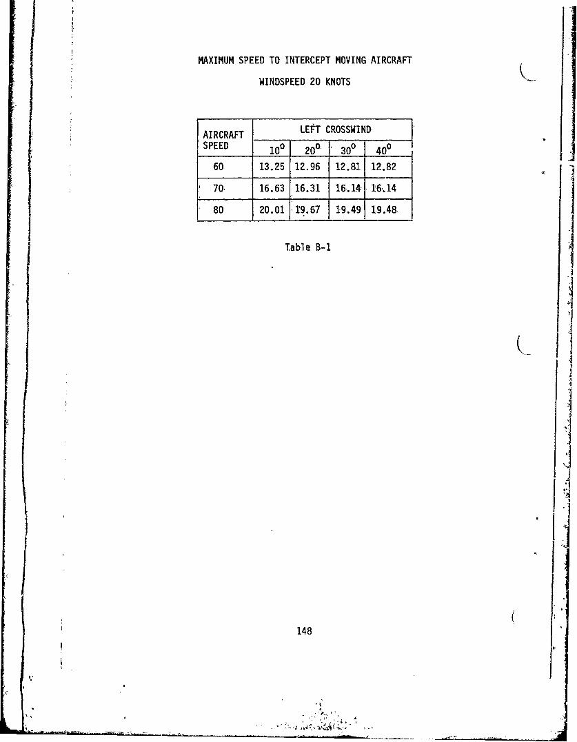
MAXIMUM SPEED TO INTERCEPT MOVING AIRCRAFT
WINDSPEED 20 KNOTS
AIRCRAFT LEFT CROSSWINDJ
SPEED 100 200 300 400
60 13.25 12.96 12.81 12.82
70 16.63 16.31 16.14, 16,.14
80 20.01 19.67 19.49 19.48,
Table B-1
148

FARTHEST POINT OF RADAR VISION
LEFT HAND TURN
400 SWEEP - 60-KNOT AIRSPEED
WINDSPEED! RIGHT CROSSWIND COMPONENT
KNOT 50 10 150 200 250 300 3r0
0 1.21.2 J. .2.2 .2 .2 .2
5 17 .17 .17 .16 .1 .16 .16 .16
10 .14 .14 .13 .13 .12 .12 .11 .11
15 .12 .II .10 .095 ,088 .082 .076 .070
20 .093 .084 .075 .065 .057 .048" .041 .033
25 .072 .061 .051 .040 030 .020 .01 .003
Table B-2
I
149
II
I.

Bibliography
1. 'Duncan, A.J. Quality Control and Industrial Statistics. ;Homewood,
Illinois': Richard D. Irwin, 1965.
2. Siegel, 'Sidney. Nonparametric Statistics for the Behavioral Sciences.
New York: McGraw-Hill, 1956.,
3. Tenenbaum, 14. and Pollard, H. Ordinary Differential Equations. New
'York,: Harper & Row, 1963.
(
150
I.7


