
An assessment of land use patterns for Genetically Modified crops in South Africa
TECHNICAL REPORT
Volume 1: A
GMO Monitoring & Research Programme
REPORT NUMBER: SANBI/GMO2016/2016/Vol1/A

CITATION FOR THIS REPORT:
Masehela, T.S., Terrapon, H., Winker, H. and Maphisa, D. An assessment of land use patterns for
Genetically Modified crops in South Africa 2016: Technical Report Volume 1: GMO Monitoring &
Research. South African National Biodiversity Institute, Newlands, Cape Town. Report Number:
SANBI/GMO2016/2016/Vol1/A
REPORT PREPARED BY:
Tlou Masehela1
Heather Terrapon1
Dr Henning Winker1
Dr David Maphisa1
1South African National Biodiversity Institute, Kirstenbosch Research Centre, 99 Rhodes Avenue,
Newlands.
Reviewers:
Zuziwe Nyareli (SANBI), Thato Mogapi (DEA), Tondani Kone (DEA), Tshifhiwa Munyai (DEA), Ntando
Mkhize (DEA), Ntakadzeni Tshidada (DEA), Muleso Kharika (DEA) and Thizwilondi Rambau (DEA)
CONTACT PERSON:
Tlou Masehela
SANBI
PO Box X7, Claremont, 7735
Tel: + 27 21 799 8702
Email: [email protected]

Table of Contents LIST OF TABLES ........................................................................................................................................... ii
LIST OF FIGURES .......................................................................................................................................... ii
LIST OF APPENDICES .................................................................................................................................... ii
EXECUTIVE SUMMARY ........................................................................................................................... 1
1. INTRODUCTION ............................................................................................................................... 2
1.1 Global status of Genetically Modified crops ................................................................................. 2
1.2 GM crops of significance: maize, cotton and soybean ................................................................. 3
1.3 Impacts of GM crops on natural areas and other crops ............................................................... 5
1.4 Documenting and monitoring GM crop land use patterns ........................................................... 6
1.5 GM crops and land use in South Africa ......................................................................................... 7
2. REPORT OBJECTIVE AND RATIONALE .............................................................................................. 9
2.1 Objective ....................................................................................................................................... 9
2.2 Rationale ....................................................................................................................................... 9
3. DATA SOURCING AND ANALYTICAL METHODS ........................................................................... 10
3.1 Data sources for GM maize and soybean ................................................................................... 10
3.2 Data sources for land cover change ............................................................................................ 10
3.3 Analysis for GM maize and soybean ........................................................................................... 11
3.4 Analysis of land cover change ..................................................................................................... 11
4. RESULTS ........................................................................................................................................ 14
4.1 GM maize and soybean ............................................................................................................... 14
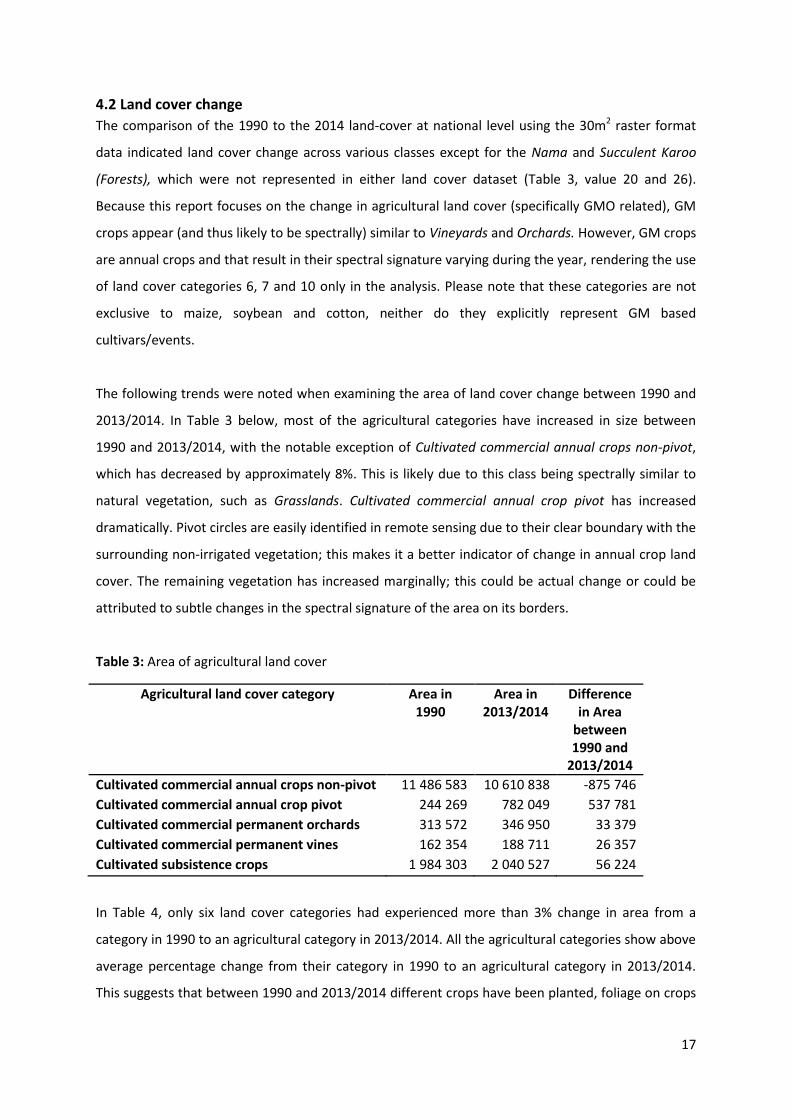
4.2 Land cover change ...................................................................................................................... 17
5. DISCUSSION .................................................................................................................................. 21
5.1 GM maize and soybean land-use area and productivity ............................................................ 21
5.2 Land cover change ...................................................................................................................... 23
6. CHALLENGES ENCOUNTERED IN COMPILING THE REPORT ......................................................... 24
7. RECOMMENDATIONS FOR MONITORING WORK ........................................................................ 25
8. REFERENCES .................................................................................................................................. 26
ii
LIST OF TABLES
Table 1: Global introduction of land-use for GM crops for the period 1996-2012 ................................ 2
Table 2: Land-use area of GM crops in South Africa, 2001 to 2010. [adjusted] ..................................... 8
Table 3: Area of agricultural land cover................................................................................................ 17
Table 4: National level land cover change to agriculture in 2013/2014 ............................................... 20
LIST OF FIGURES
Figure 1: GM cotton, maize and soybean share in the total acreage (million hectares) of a country
from 1997 – 2013. Source: GMO Compass (2014). ................................................................................ 4
Figure 2: Analysis of land cover change indicating the changed area between 1990 and 2014. This
resulted in a layer which showed the land cover in 1990 (2a) that changed to agriculture in 2014 (2c).
The visual process for the change can be observed in 2b. ................................................................... 13
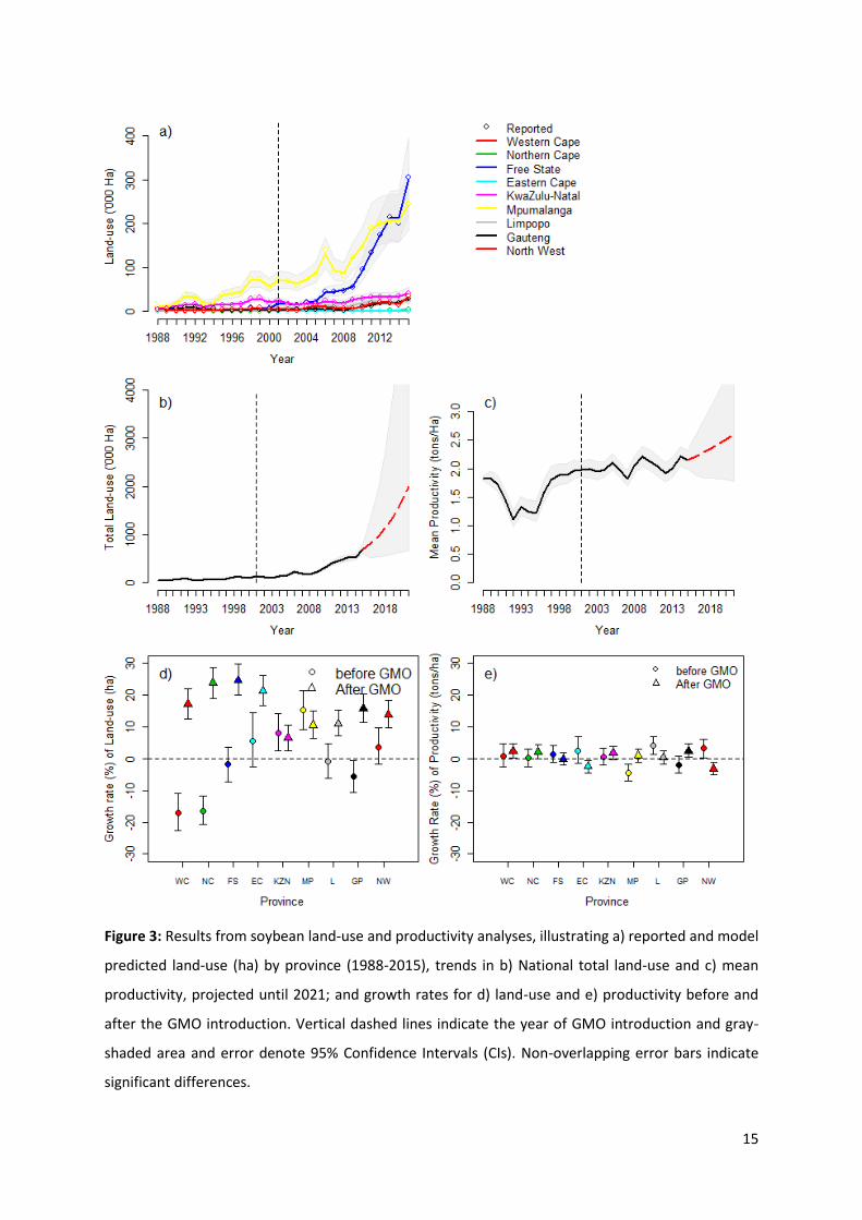
Figure 3: Results from soybean land-use and productivity analyses, illustrating a) reported and model
predicted land-use (ha) by province (1988-2015), trends in b) National total land-use and c) mean
productivity, projected until 2021; and growth rates for d) land-use and e) productivity before and
after the GMO introduction. Vertical dashed lines indicate the year of GMO introduction and gray-
shaded area and error denote 95% Confidence Intervals (CIs). Non-overlapping error bars indicate
significant differences. .......................................................................................................................... 15
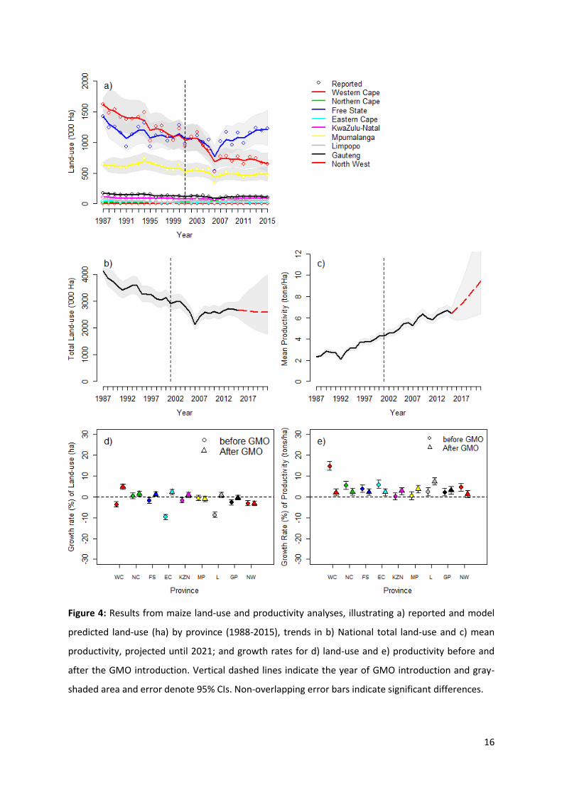
Figure 4: Results from maize land-use and productivity analyses, illustrating a) reported and model
predicted land-use (ha) by province (1988-2015), trends in b) National total land-use and c) mean
productivity, projected until 2021; and growth rates for d) land-use and e) productivity before and
after the GMO introduction. Vertical dashed lines indicate the year of GMO introduction and gray-
shaded area and error denote 95% CIs. Non-overlapping error bars indicate significant differences. 16
LIST OF APPENDICES
Appendix 1: Table 5 used for reporting land cover change for inter-classes and national level. ........ 30
Appendix 2: Outline of variables and parameters for the Bayesian State Space model (BSPM)
framework for GM maize and soybean data analysis........................................................................... 31
Appendix 3: Comparison of agricultural areas between 1990 and 2013/2014. .................................. 33
Appendix 4: Vector based agricultural fields, derived from the Agricultural Field boundary data
captured by SIQ. .................................................................................................................................... 35

1
EXECUTIVE SUMMARY
The global area of cultivation for Genetically Modified (GM) crops, also referred to as Biotech crops,
has increased significantly since their adoption and commercial purposes began in the mid-nineties.
Although the trade-offs between benefits and adverse effects of GM crops (and other Genetically
Modified Organisms – GMOs) are still debatable globally, there is increasing interest from various
countries to adopt GM crops because of the anticipated benefits for crop production. South Africa,
one of the leading GM crop growing countries globally, has a total of 2.7 million hectares under GM
cotton, maize and soybean production. These have all been approved for general release. However,
the growth in cultivation areas over the years has not been evaluated in terms of the effects on land-
use and productivity trends as well as land cover change, with potential impacts thereof being
unknown. For the purpose of this report, we gathered annual production area data (in hectares) for
cotton, maize and soybean. We explored trends in land-use and productivity using a Bayesian State
Space Model (BSPM) for maize and soybean pre- and post-introduction of GM traits (events).
Currently, available cotton data was discarded due to various irregularities and an insufficiently long
time series. In addition, land cover change from 1990-2014 was explored using the 2013-2014 South
African National Land-cover dataset produced by GEOTERRAIMAGE with comparison of vector based
agricultural fields being the main priority. The GEOTERRIAMAGE Report was used to infer on land
use-land cover change impact to contextualise some of our findings.
Results show an overall acceleration in increase of land-use for soybean since the introduction of
GM traits. Maize land-use area has experienced some declines but seem to be fairly constant in
recent years. These trends are, however, highly variable at provincial levels, with several provinces
making gains while others remain on a stable trend in production areas. Productivity output in ton
per hectare has consistently increased for both maize and soybean, but no significant acceleration
effect of this trend was detected post GM introductions. Land cover changes show an increase for
cultivated commercial annual crops pivot and cultivated subsistence crops, as opposed to cultivated
commercial annual crops non-pivot. Grasslands are the most affected in area loss resulting from
these cultivation increases. However, based on the available data it was not possible to directly
attribute this emerging pattern to GM crops, since the respective cultivation areas are inclusive of
other crop types. Further analysis using disaggregated annual provincial production area data for
GM crops is essential for producing more accurate trends and predictions before any conclusions
can be reached for the effect of GM crops on land-use, productivity and land cover change. Further
analyses will enable the detection of any GM crop cultivation decreases and/or increases that impact
directly on land cover for each province.

2
1. INTRODUCTION
1.1 Global status of Genetically Modified crops
Genetically Modified (GM) crops are modified using genetic engineering techniques to introduce a
new trait to the plant, which does not occur naturally in the species (Southgate et al. 1995). These
plants can either be food crops, pharmaceutical agents, biofuels and those used for bioremediation.
For GM crops in particular, newly introduced traits are designed to improve nutrient profile of the
crop or protect the crop from certain pests, diseases and environmental conditions (Wieczorek 2003;
James 2013). The adoption of GM crops globally for commercial purposes began around 1995/6,
covering 1.7 million hectares (Table 1). By 2012, GM crops covered 170.3 million hectares (Table 1).
The most recent period (2005-2012) indicated acceleration in the increase in area-use for GM crops
from 90 to 130 million hectares, resulting in almost a doubling of GM crop land-use (James 2013).
Table 1: Global introduction of land-use for GM crops for the period 1996-2012
Year Hectares (million) Acres (million)
1996 1.7 4.3
1997 11 27.5
1998 27.8 69.5
1999 39.9 98.6
2000 44.2 109.2
2001 52.6 130
2002 58.7 145
2003 67.7 167.2
2004 81 200
2005 90 222
2006 102 252
2007 114.3 282
2008 125 308.8
2009 134 335
2010 148 365
2011 160 395
2012 170.3 420
Total 1427.3 3531.8
Source: Clive James (2012)
GM crop cultivation area has since reached 181.5 million hectares in the year 2014, an increase of
6.3 million hectares from 175.2 million hectares in 2013 (James 2014). However, the uptake of GM
3
crops is highly variable among countries, with developing countries having a more rapid uptake. The
United States of America (USA), Brazil, Argentina, India and Canada remain the top five countries
globally for the largest area of GM crop production (James 2014). South Africa ranks ninth in the
world and first in Africa in terms of area of GM crop production.
1.2 GM crops of significance: maize, cotton and soybean
Globally, maize soybean and cotton are the most widely adopted and cultivated GM crops.
According to the 2014 International Service for the Acquisition of Agri-biotech Applications (ISAAA)
report, GM maize is cultivated in 17 of the 28 countries that have adopted GM crops while cotton is
cultivated 15 (James 2014). These remained unchanged from 2013 (refer to James 2013). Although
there was one additional country that adopted a GM crop (bringing the total to 28), in Bangladesh,
the approval was for the cultivation of Brinjal/Eggplant. A recent report by the Canadian
Biotechnology Action Network (CBAN) shows that half of the global area used is planted with GM
soybeans. GM corn accounts for 30% of the total global GM area coverage and GM cotton accounts
for another 14% and GM canola accounts for 5% of the total GM land-us. The cultivation and use of
maize, soybean and cotton varies in different countries. Maize is one of the most important cereal
crops worldwide and is not only an important human nutrient, but also a basic element of animal
feed and a raw material for the manufacture of many industrial products (Shaw 1988; Ranum et al.
2014). Soybean uses range from production of soybean oil, provision of meals for human
consumption (i.e. flour and infant formula) to production of animal feed (FAO 2006). Cotton is
mostly referred to as a cash crop, due to its high preference for fibre (Proto et al. 2000). Other uses
of cotton include the production of cooking oil and feed for livestock, poultry and fish (Chapagain et
al. 2006).
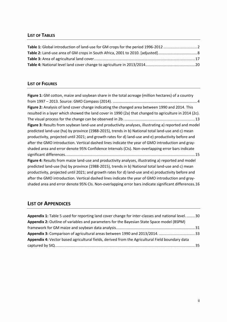
The GMO Compass (2014) reports on the cultivation of GM cotton, maize and soybean from 1997-
2013 (Figure 1). Their analysis divided the data into worldwide (other countries) and the top three
producing countries for the respective crops. Results from the aforementioned analysis showed that,
after initial sharp increases in the early years, land-use of GM cotton plateaued around 2000-2003 in
the USA and China, with only a small increase since then. India experienced a delayed, but rapid
decrease in cotton land use between 2005 and 2009. At a global scale, the increase in cotton land-
use was steady and approximately linear from 1997 before a slight decrease in 2013. Genetically
Modified Maize land-use increased throughout 1997-2013 for South Africa. The USA experienced a
constant increase in GM maize land-use for most years except during 2000 and 2013. Soybean
acreage for the USA peaked from 1997, experienced a decrease in 2009, picking up consistently from

4
2010 to 2013. This trend was almost similar to that of Argentina, although the decrease for
Argentina occurred in 2004, before levelling off from 2005 to 2010 with a slight increase until 2013.
Worldwide acreage for soybean increased for all years, with decreases only experienced for 2011
and 2013. For Brazil, a decrease in land-use was only experienced during 2002-2003.
Annual acreage increases or decreases are mostly controlled by factors relating to: 1) uncertainties
in climatic conditions; 2) market trends (supply versus demand) related to the economic climate,
public perceptions and lobbying by different organisations (i.e. anti-GMO groups); 3) development of
new/favourable cultivars resulting in farmer preferences; and 4) changes in regulations that affect
both exporting and importing countries (see James 2014; Lucht 2015).
Figure 1: GM cotton, maize and soybean share in the total acreage (million hectares) of a country from 1997 – 2013. Source: GMO Compass (2014).
The global increase in the adoption and cultivation of GM crops has been credited to the perception
of the technology as a powerful tool for efficient contribution in agriculture production (James
GM cotton GM soybean
GM maize

5
2014). Reviews by Carpenter (2010), Finger et al. (2011), Green (2012), Klumper & Qaim (2014),
indicate some benefits relating to reduced chemical pesticide use, increased crop yields and
increased farmer profits. These benefits can be attributed to favourable properties of GM crops for
improving pest management, therefore reducing or eliminating losses from insect damage or weed
competition, thus indirectly improving yields substantially. Also, increases in crop yields allow less
land to be dedicated to agriculture than would otherwise be necessary (Carpenter 2011). In contrast,
there is a multitude of concerns about the impact of GM crops on the environment (Wolfenbarger et
al. 2000; Garcia & Altieri 2005; Mannion & Morse 2013). Key issues in the environmental assessment
of GM crops are putative invasiveness, vertical or horizontal gene flow, other ecological impacts,
effects on biodiversity and the impact of presence of GM material in other products (see Hails 2000;
Poppy 2000; Conner et al. 2003; Prasifka et al. 2007; Bøhn et al. 2008; Lang & Otto 2010; Cambers et
al. 2010).
1.3 Impacts of GM crops on natural areas and other crops
Agricultural practices are generally documented to have negative impacts on the environment (see
Moorehead & Woolmer 2001; Firbank et al. 2008, Power 2010). In relation to GM crops and land,
Brookes & Barfoot (2010) found that more land would be converted into agricultural use were it not
for various GM crops traits. James (2014) also supports this, indicating that GM crops contribute
towards biodiversity conservation. He further alludes that biotechnology (biotech; equivalent to GM
crops) crops are a land-saving technology, capable of higher productivity on arable land, and thereby
can help preclude deforestation and protect biodiversity in forests and in other in-situ biodiversity
sanctuaries. Furthermore, if the additional high output tonnage of food, feed and fibre produced by
biotech crops during the period 1996 to 2013 had not been produced by biotech crops, an additional
132 million hectares of conventional crops would have been required to produce the same tonnage.
In essence, James (2014) demonstrates that the use of GM crops for high yields is highly viable over
small acreage.
At the same time, GM crops can also encourage increases in crop land-use, particularly where
farmers decide to increase acreage planted with GM crops at the expenses of other farming
activities or through expansion into natural areas (Carpenter 2011; Brookes et al. 2010.). In their
report, Bindraban et al. (2009) used an increase in GM soybean production in Latin America to
illustrate its impacts on natural areas. They concluded that GM soybean impacted negatively on
natural areas as the increase in production areas led to the conversion of conservation (natural) and
pasture areas into arable land for soybean production. This also had a ripple effect on livestock
6
farmers in the area as they also expanded their practice to other natural areas to sustain their
farming. Similar trends were also observed in Argentina, Paraguay and Brazil relating to soybean and
maize, whereby the cultivation of GM soybean contributed directly and indirectly to the loss of
natural areas. Not only do GM crops result in loss of natural areas, they can also replace other crops
when used as season cash crops (see Bindraban et al. 2009). For example, in Argentina, increases in
GM soybean production resulted in the loss of various pastures and areas used for maize cultivation
as opposed to natural areas (Bindraban et al. 2009).
1.4 Documenting and monitoring GM crop land use patterns
The assessment of agricultural productivity levels and trends is important given that the amount and
composition of agricultural output of a particular country or region of the world tends to change
over time (Brady & Sohngen 2008). Moreover, spatial dynamics of agriculture can be complex where
data is inadequate or non-existent. At times, influential factors relating to weather and climate, soils,
and pest pressures might need to be considered when assessing decreases and increases in
agricultural land use. Consequently, agricultural expansion, production and productivity can be
influenced by other factors (natural), as opposed to just the desire to adopt a particular technology.
However, recent trends outlining increases in global GM crop production areas (James 2012, 2013
and 2014) creates an assumption that the technology has brought about benefits that promotes
expansion of agricultural areas. Although, conventional and organic farming does lead to an increase
in production area (Dimitri & Greene 2002), increases resulting from the uptake of GM crops has
been rather rapid. At the same time, GM crops are depicted to have high outputs (yields) at smaller
planting scales (see section on GM crops and land use). Ausubel et al. (2013) also alludes to
combinations of agricultural technologies which have raised yields, keeping downward pressure on
the extent of cropland, and therefore sparing land for nature.
Perhaps a question to then ask would be “if the planting area of GM crops is increasing annually (in
terms of acreage), is the increase at the expense of other agricultural crops or the clearing of natural
areas and degraded areas?” Examples from Latin America, Argentina, Paraguay and Brazil indicate all
three scenarios to be possible (Bindraban et al. 2009). But what are the implications for each of
these scenarios? Concerns range from carbon loss and climate change, biodiversity loss to top soil
loss, and many others (Brady & Sohngen 2008). Given the mismatches in benefits and negative
impacts of GM crops regarding increases in land use area, it is highly imperative to document,
monitor and report GM crops activities in relation to production area.
7
1.5 GM crops and land use in South Africa
South Africa approved its first GM crops for commercial release between 1997 and 2005 (Wolson
2007). Some of the initial traits/events approved included Insect-resistant cotton, Insect-resistant
maize (yellow), Herbicide-tolerant cotton, Herbicide-tolerant soybeans, Herbicide-tolerant maize
and Stacked-gene cotton (insect resistance and herbicide tolerance) (refer to DAFF 2005; Wolson &
Gouse 2005). To date, South Africa has approved a total of 67 events. Argentine Canola - Brassica
napus has four (4) events, Cotton - Gossypium hirsutum L. 10 events, Maize - Zea mays L.: 40 events,
Rice - Oryza sativa L.: one (1) Event and Soybean - Glycine max L.: 12 events. However, both canola
and rice were only approved for commodity clearance (i.e. processing for human consumption and
animal feed) in 2001 and 2011 respectively, as opposed to cotton, maize and soybean permits
ranging from field trials to commercial planting
(http://www.daff.gov.za/daffweb3/Branches/Agricultural-Production-Health-Food-Safety/Genetic-
Resources/Biosafety/Information/Permits-Issued).
There is a general perception that the area under GM crop cultivation in South Africa increases
annually as a result of planting GM maize, cotton and soybean. The ISAAA 2010 confirms this by
outlining GM crops plating area from 2001-2010 (Table 2). The total area of GM crops increased
from 197 thousand hectares in 2001 to 2.2 million hectares in 2010. The report also makes special
mention on total area increases in white GM maize production. It is shown that total area of GM
maize increase from 166 thousand hectares in 2001 to 1.9 million hectares in 2010. This indicates
that GM maize accounted for more than 85% of the total production area of GM crops in South
Africa. The increase in total production area increased to 2.2 million hectares in 2011 (James 2011),
increased to 2.9 million hectares in 2012 (James 2012) and remained unchanged in 2013 (James
2013), then decreased to 2.7 million hectares in 2014 (James 2014).

8
Table 2: Land-use area of GM crops in South Africa, 2001 to 2010. [adjusted]
Year
Total land-use of maize, soybean
and cotton (million hectares)
Total land-use of GM maize
(million hectares)
Total land-use of GM white maize
(million hectares)
Percentage of GM white
maize of total white maize
area
2001 19.7 16.6 0.6 < 1%
2002 27.3 23.6 6.0 3%
2003 40.4 34.1 14.4 8%
2004 57.3 41.0 14.7 8%
2005 61.0 45.6 28.1 29%
2006 1412 1232 704 44%
2007 1800 1607 1040 62%
2008 1813 1617 891 56%
2009 2116 1878 121 79%
2010 2229 1898 1139 75%
Total 11427 9841 5624
Source: Compiled by ISAAA, 2010
These increases in GM crop production area, with the exception of a decrease in 2014, might be a
good indication in terms of the technology adoption and its positive attributes. At the same time, it
poses a dilemma of determining if the increases take place at the expense of natural areas or other
crops (cultivated land). Schoeman et al. (2013) conducted a study to determine the extent of
transformed landscape change within South Africa over a 10-year period between 1994 and 2005.
Using five classes of land cover change (Urban, Mining, Forestry, Cultivation and Other) they
concluded that at a national level there has been a total increase of 1.2 % in transformed land
specifically associated with Urban, Cultivation, Plantation Forestry and Mining. On a finer national
scale, cultivated land had decreased from 12.4% to 11.9%. When considering these findings, it is
difficult to ascertain where the increases in GM crop area outlined in Table 2 took place. The logical
explanation here could be that GM crops expanded at the expense of other commercial crops, but
this is difficult to prove without any data. It is for this reason that Schoeman et al. (2013)
recommend that any research on change in land cover should include investigation into the
transformed cover classes with the objective of identifying the drivers and type of change that has
occurred, as well as the social, environmental and economic impacts of these changes over time.

9
2. REPORT OBJECTIVE AND RATIONALE
2.1 Objective
Based on various aforementioned reports, the GM crop production area is increasing in South Africa,
but there is considerable uncertainty regarding the impact that this has on land use or land cover
change. Possible scenarios of the increases are that farmers are either expanding into natural
vegetation or opting not to plant other crops that they used to plant before. The objective of this
report was to conduct an analysis to: 1) predict and forecast underlying trends in land-use and
productivity; and 2) to evaluate if the introduction of GM maize and soybean seeds to South Africa in
1998 and 2001, respectively, had a significant effect on the land-use and production trends. For this
preliminary report, GM cotton data was discarded due to data availability for analysis representing
only post GM seed introduction years for the period 2004-2015. This precluded a comparison of pre
and post GM introduction trends for both land use and productivity. The report also gives a brief
account of land cover change between 1990 and 2014.
2.2 Rationale
Analysis findings will enable an understanding in GM land-use and production trends for cotton,
soybean and maize to improve predictions of future trends and related impacts on land-use and land
cover. Improved reporting and monitoring can be initiated as part of environmental management
and conservation strategies where applicable.
10
3. DATA SOURCING AND ANALYTICAL METHODS
3.1 Data sources for GM maize and soybean
Annual South African census data on land-use in hectares (ha) and productivity in tons per hectare
(tons/ha) of maize and soybean were sourced for the period 1987 to 2016 – this data is collected
annually for these and other crops. Data was provided by the Crop Estimates Committee (CEC), a
Branch of the Department of Agriculture, Forestry and Fisheries (DAFF). These annual figures were
separately reported per provinces, but data were incomplete for the Western- and Eastern Cape,
with some years missing figures. The current year (i.e. 2016) was excluded from the analysis because
of likely underestimates of total land-use due to incomplete cycles. Similarly, the soybean data for
1987 were largely missing or appeared to be lacking as a result of underreporting and were
therefore omitted. Initial analysis trials showed, however, that this had little effect on the overall
trends.
3.2 Data sources for land cover change
The land cover analysis made use of the South African National land Cover datasets (Department of
Environmental Affairs, 2014) for 2009 and 2013/2014. These datasets were produced by
GEOTERRAIMAGE and an open license has been purchased by the Department of Environmental
Affairs (DEA) in this regard. The datasets have been generated from digital, multi-seasonal Landsat 8
multispectral imagery, acquired between April 2013 and March 2014 and 1990 and 1991.
For comparison of vector based agricultural fields, the Agricultural Field boundary data captured by
SIQ (Spatial IQ, 2014) was obtained from DAFF. A previous version of the data offered a second point
in time. Please note that the date of data capture for the datasets varies (refer to Appendix 1). The
data encompasses all the field crop boundaries in the provinces of South Africa. Field crop
boundaries are defined as the result of different cropping patterns within one field boundary,
planting different crops or the same crop at different planting dates. This separation is not always
fixed, and could vary from year to year. The dataset was developed to serve as the sampling frame
dataset for the Producer Independent Crop Estimation System (PICES) for the provinces. PICES is a
system developed by the National Crop Statistics Consortium (NCSC) which utilises in-season
satellite imagery combined with a point frame statistical methodology to objectively determine the
area under grain crops in a province.

11
3.3 Analysis for GM maize and soybean
A Bayesian State Space model (BSPM) framework (Meyer and Millar 1999) was implemented for the
trend analysis of land-use (area occupied) and productivity (production per hectare) for soybean and
maize. The BSPM represents a powerful tool for time series analysis (de Valpine 2002), which allows
accounting for both process error (environmental year to year variation) and potential reporting
error (Thorson et al. 2014). The BSPM was fitted to the reported land-use (ha) and production
(tons/ha) data per province. The change in the trend determined by the response variable Y (i.e.
land-use or productivity) follows a Markovian process, which means that, for example, Yt+1 in the
following year t + 1 will depend on the Yt in the current year t (Kery & Michael Schaub 2012).
Responses for each variable (i.e. Y for crop type), crop type, land use (metric) and province are
explained further in Appendix 2. Bayesian credibility intervals for the model used are also accounted
for.
3.4 Analysis of land cover change
Three methods were used to analyse spatial change in agriculture. The first was to review the report
made by GEOTERRAIMAGE on all categories of land cover change between 1990 and 2013 in South
Africa (Department of Environmental Affairs, 2014), see Appendix 1 to view the pertinent table listed
in the report. The second was to analyse the spatial data underlying this report with the aim to
focus on the change of land cover to agricultural land use in 2013/2014 only. The third method made
use of vector data showing the agricultural field boundaries and compared boundaries captured in
2007 to those captured in 2011.
The comparison of the two land cover data sets was problematic in that they are each big in size
(approximately 4 Gigabyte), therefore compromising the computational analysis power. The
methodology had to prioritise the reduction of the data file size in order to process the final result.
The symmetric difference tool (Diff function) in ArcGIS Spatial Analyst was used to compute the
difference between the two land covers. This function created a data layer showing the land cover
values for 1990 that were different from the values in 2014. The 2014 land cover was then
reclassified to show only those classes pertaining to agriculture. The resultant layer was used to
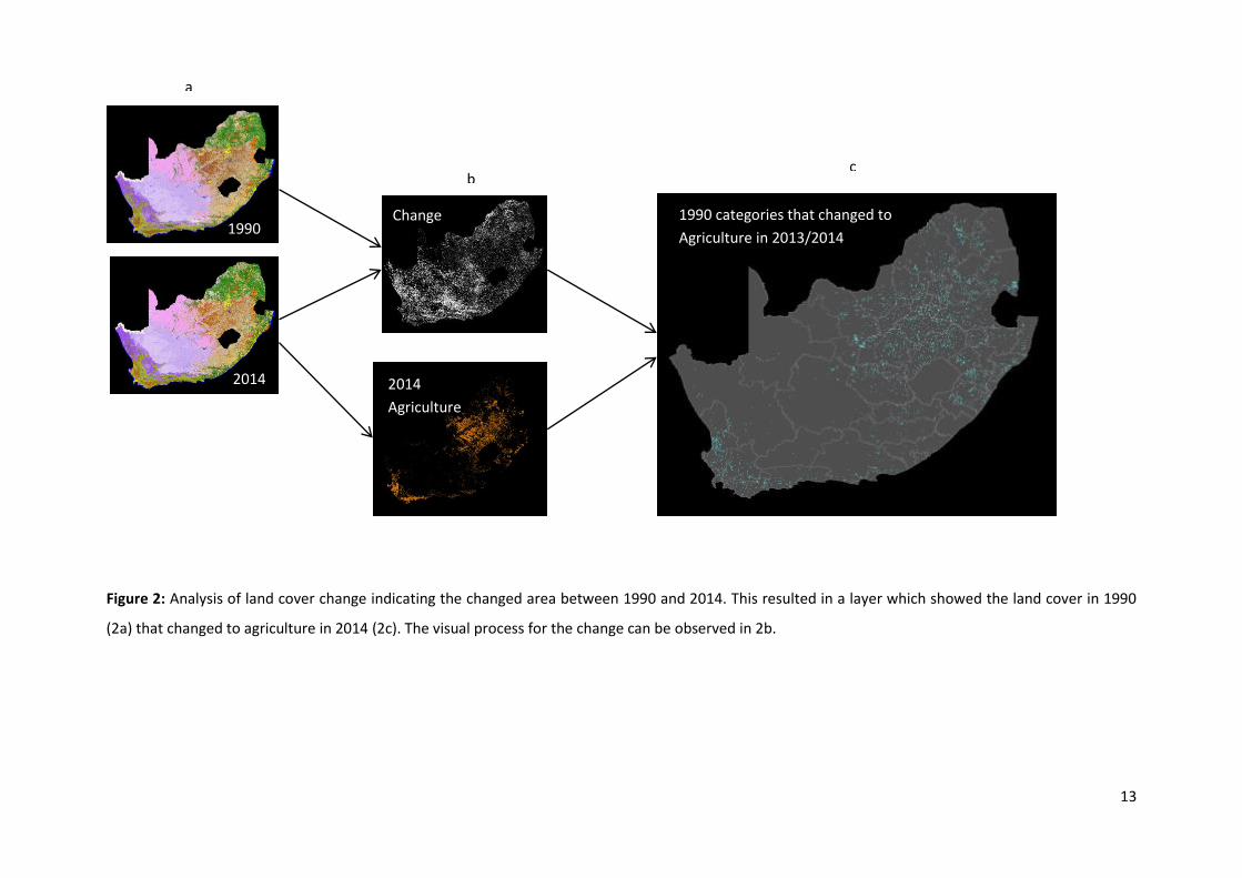
extract the changed area between 1990 and 2014. This resulted in a layer which showed the land
cover in 1990 that changed to agriculture in 2014; see Figure 2 below for a visual representation of
this process. A table was created by multiplying the number of raster cells in a land cover category
by the cell size (30m2). This was done for the changed area, as well as the area in 1990 and 2014. The
changed area in the table only shows how much of the land cover have changed to agriculture;
12
changes between other land cover categories between 1990 and 2014 are not shown. These land
cover datasets were generated using remote sensing and vector data and which has an approximate
accuracy of 85%. With this accuracy in mind, it is worth noting that the least accurate categories are
Natural vegetation categories, Bare ground and Built up areas (Department of Environmental Affairs
2014). Thus the resulting areas of change to agriculture should only be seen as an approximation.
For comparison of vector based agricultural fields, a symmetrical difference function was used to
overlay the two datasets (metadata for 2007 – 2010 and metadata for the data for 2011) with the
results showing areas where the two datasets were did not coincide. Also see Appendix 3 for
additional comparison figures of agricultural areas between 1990 and 2013/2014. The following
columns were created in the dataset:
OArea: Original polygon area (original area of the crop)
NArea: New area (calculated area of the polygon showing the difference between the layers)
Type: Agriculture type (contains any descriptive information form either layer about what
agriculture is happening in the polygon)
Captured: Year that the polygon was captured
Refer to notes in Appendix 4 for further information on the identification of new fields, and data
errors which were likely to be the result of spatial data capture corrections.
13
Figure 2: Analysis of land cover change indicating the changed area between 1990 and 2014. This resulted in a layer which showed the land cover in 1990
(2a) that changed to agriculture in 2014 (2c). The visual process for the change can be observed in 2b.
1990
2014
Change
2014
Agriculture
1990 categories that changed to
Agriculture in 2013/2014
a
b c
14
4. RESULTS
4.1 GM maize and soybean
Patterns in land-use (ha) and productivity (ha/tons) showed substantially different patterns for
soybean and maize (Figures 3 and 4). The top two provinces in terms of land-use for soybean were
the Free State and Mpumalanga (Figures 3a). For maize, Free State, North West and Mpumalanga
had the highest land use (Figure 4a). However, both North West and Mpumalanga show a decrease
in maize area in the early 2000s’ onwards (Figure 4a). The Western and Northern Cape provinces had
the lowest land-use for both crops in general.
On a national scale, land-use for soybean showed a substantial increase at a rate of 13% per annum.
At this rate, it was predicted that there is 50% probability that total land-use for soybean will exceed
2 million hectares by 2021 (Figure 3b). The national land-use trend for maize showed a consistent
decline until 2007, but appeared to have stabilized thereafter. Projections at current rates suggest a
minimal decline by less than 1% per annum and therefore fairly constant land-use until 2021 (Figure
4b). The national average in productivity (i.e. production in tons per hectare) has increased since
1988. Soybean productivity was lowest between 1992 and 1995, but recovered quickly in 1996 to
the 1990 levels, and increased consistently since then at a fairly low average rate of increase of 0.5%
per annum (Figure 3c). Maize productivity, by contrast, showed a steeper and almost linear trend of
increase with an estimated annual rate of growth in productivity by 3.7% (Figure 4c).
The introduction of GM soybean in 2001 resulted in significant increases in land-use trends for a
number of provinces (Figure 3d). Among the three provinces with the highest land-use for soybean,
only the Free State showed significant increase after the GM introduction by close to 23%, whereas
Mpumalanga and Kwazulu-Natal revealed no acceleration of the land-use trend (Figure 3d). Notably,
the provinces with very low overall land-use showed the highest increase after the GM introduction.
In contrast, to observed change in the rate of increase in land-use, none of the provinces, but
Mpumalanga (+5%), showed a significant increase in productivity compared to the long-term trend
(Figure 3e). The introduction of GM maize in 1998 resulted in significant increases in the land-use
trends for Western-Cape, Eastern Cape, and Gauteng (Figure 4d). Therefore, the provinces, which
are among the least important for national maize production, indicated an increase in land-use
following the GM introduction, whereas the main producing provinces showed no divergence from
the fairly stable long-term trend in land-use for maize. Similar to soybean productivity, no significant
increase in maize productivity per hectare land was detected.
15
Figure 3: Results from soybean land-use and productivity analyses, illustrating a) reported and model
predicted land-use (ha) by province (1988-2015), trends in b) National total land-use and c) mean
productivity, projected until 2021; and growth rates for d) land-use and e) productivity before and
after the GMO introduction. Vertical dashed lines indicate the year of GMO introduction and gray-
shaded area and error denote 95% Confidence Intervals (CIs). Non-overlapping error bars indicate
significant differences.
16
Figure 4: Results from maize land-use and productivity analyses, illustrating a) reported and model
predicted land-use (ha) by province (1988-2015), trends in b) National total land-use and c) mean
productivity, projected until 2021; and growth rates for d) land-use and e) productivity before and
after the GMO introduction. Vertical dashed lines indicate the year of GMO introduction and gray-
shaded area and error denote 95% CIs. Non-overlapping error bars indicate significant differences.
17
4.2 Land cover change
The comparison of the 1990 to the 2014 land-cover at national level using the 30m2 raster format
data indicated land cover change across various classes except for the Nama and Succulent Karoo
(Forests), which were not represented in either land cover dataset (Table 3, value 20 and 26).
Because this report focuses on the change in agricultural land cover (specifically GMO related), GM
crops appear (and thus likely to be spectrally) similar to Vineyards and Orchards. However, GM crops
are annual crops and that result in their spectral signature varying during the year, rendering the use
of land cover categories 6, 7 and 10 only in the analysis. Please note that these categories are not
exclusive to maize, soybean and cotton, neither do they explicitly represent GM based
cultivars/events.
The following trends were noted when examining the area of land cover change between 1990 and
2013/2014. In Table 3 below, most of the agricultural categories have increased in size between
1990 and 2013/2014, with the notable exception of Cultivated commercial annual crops non-pivot,
which has decreased by approximately 8%. This is likely due to this class being spectrally similar to
natural vegetation, such as Grasslands. Cultivated commercial annual crop pivot has increased
dramatically. Pivot circles are easily identified in remote sensing due to their clear boundary with the
surrounding non-irrigated vegetation; this makes it a better indicator of change in annual crop land
cover. The remaining vegetation has increased marginally; this could be actual change or could be
attributed to subtle changes in the spectral signature of the area on its borders.
Table 3: Area of agricultural land cover
Agricultural land cover category Area in 1990
Area in 2013/2014
Difference in Area
between 1990 and
2013/2014
Cultivated commercial annual crops non-pivot 11 486 583 10 610 838 -875 746
Cultivated commercial annual crop pivot 244 269 782 049 537 781
Cultivated commercial permanent orchards 313 572 346 950 33 379
Cultivated commercial permanent vines 162 354 188 711 26 357
Cultivated subsistence crops 1 984 303 2 040 527 56 224
In Table 4, only six land cover categories had experienced more than 3% change in area from a
category in 1990 to an agricultural category in 2013/2014. All the agricultural categories show above
average percentage change from their category in 1990 to an agricultural category in 2013/2014.
This suggests that between 1990 and 2013/2014 different crops have been planted, foliage on crops

18
has increased, thus altering the spectral signature of the crop, or irrigation has been installed in the
field. Wetlands have shown a high percentage of conversion to agriculture, these areas do have
richer soil and are more abundant in water and so are likely to be cultivated. However wetter
seasonal conditions in 1990 resulted in Wetlands being more easily identified in 1990 than the
2013/2014 imagery. Wetlands may have been misclassified in 2013/2014 since they were drier than
in the 1990 imagery. Lastly, Fynbos and grassland areas have shown a high percentage of conversion
to agriculture, these areas are likely to be cultivated. However it has been noted that the Grassland
was problematic to model in the land cover dataset (Department of Environmental Affairs 2014).
The figures shown in the GEOTERRAIMAGE land cover change report (Department of Environmental
Affairs 2014) support the findings in the previous paragraph. With Cultivated commercial annual:
non-pivot being classified as one of the other agricultural categories in 1990 or as Wetlands or
Grasslands. A notable change identified in 2013/2014 is Cultivated subsidence crops being identified
as degraded areas in 1990. It is possible that this is an indication of a 4% increase in subsistence
agriculture.
20
Table 4: National level land cover change to agriculture in 2013/2014
Land cover category in 1990 Area in 1990
Area changed to Agriculture
% Change to Agriculture in 2013/2014
Indigenous Forest 346291 1324 0.38%
Thicket /Dense bush 5916089 122513 2.07%
Woodland/Open bush 9788274 132987 1.36%
Low shrub land 18278554 136006 0.74%
Plantations / Woodlots 1922819 33400 1.74%
Cultivated commercial annual crops non-pivot 11486583 429743 3.74%
Cultivated commercial annual crop pivot 244269 29319 12.00%
Cultivated commercial permanent orchards 313572 31827 10.15%
Cultivated commercial permanent vines 162354 6912 4.26%
Cultivated subsistence crops 1984303 49955 2.52%
Settlements 2742920 19011 0.69%
Wetlands 1526138 58534 3.84%
Grasslands 25317439 678951 2.68%
Fynbos: forest 30360 213 0.70%
Fynbos: thicket 283922 8141 2.87%
Fynbos: open bush 211541 3951 1.87%
Fynbos: low shrub 5919755 142767 2.41%
Fynbos: grassland 534043 21746 4.07%
Fynbos: bare ground 149179 569 0.38%
Nama Karoo: forest 0 0
Nama Karoo: thicket 170367 4656 2.73%
Nama Karoo: open bush 520970 4076 0.78%
Nama Karoo: low shrub 12893194 36805 0.29%
Nama Karoo: grassland 1222157 12942 1.06%
Nama Karoo: bare ground 10561152 5070 0.05%
Succulent Karoo: forest 0 0
Succulent Karoo: thicket 275606 3174 1.15%
Succulent Karoo: open bush 487004 3074 0.63%
Succulent Karoo: low shrub 4048359 5964 0.15%
Succulent Karoo: grassland 417329 3044 0.73%
Succulent Karoo: bare ground 1702221 514 0.03%
Mines 291757 1231 0.42%
Waterbodies 2202041 4369 0.20%
Bare Ground 1489898 1585 0.11%
Degraded 1489360 23710 1.59%
21
5. DISCUSSION
5.1 GM maize and soybean land-use area and productivity
Genetically modified crops have been adopted rapidly and cultivated commercially in a numbers of
countries over the past 23 years (Aldemita et al. 2015). The results presented in Figures 3 and 4
illustrate the trends in local land-use for both soybean and maize, respectively. Soybean had a
considerably smaller production area pre GM introduction. The opposite was true for maize.
Soybean production increased substantially over the years and predictions indicated even higher
increases in the future. In contrast, maize tends to go through gradual declines and increases over
certain periods. Similar trends are observed in other countries for both crops (see Figure 1). Locally,
maize and soybean are typically grown in the same season as their climatic requirements are similar.
However, soybeans flower over a long period, which makes them less susceptible to drought during
this stage than maize (Pannar 2006). This may be a possible explanation in the fluctuation decreases
in land use for maize cultivation in certain years (i.e. 1998-2007) versus soybean. These years were
possibly drought prone seasons. Worth noting is the steady increase in maize production post 2007,
likely due to improving rain conditions and transgenic seeds. It is also not surprising that land under
soybean production increased substantially post 1997, after the enacting of the Genetically Modified
Organisms Act (Act no. 15 of 1997) and its subsequent amendments Genetically Modified Organisms
Act Amendment (Act no. 23 of 2006). Dlamini et al. (2015), report that between 1997/8 and 2012,
land set aside for soybeans increased from 93 790 ha to 472 000 ha due to an increase in the supply
of quality transgenic seed. Our analysis here indicates that soybean production area has a 50%
chance of reaching 2 million hectares by 2021. This means the production area would have increased
three folds since 2012. For maize, however, a fairly constant land use is forecast.
Because this analysis took into account fluctuations in environmental conditions (e.g. caused by
yearly rainfall variations), a possible scenario is that if dryer conditions persist, inhibiting growth in
maize production area, soybean is likely to replace maize in most areas (provinces) across the
country, unless additional areas would be cleared to accommodate the predicted expansion based
on the current trend. Maize and soybean economic and nutrition importance differs significantly
within the African continent, but the demand for soybean is well established in South Africa and
throughout the Southern Africa Development Community (SADC) (Opperman & Varia 2011). Given
the current drought conditions, most farmers are likely to opt to producing soybean compared to
maize. This would imply that areas previously under maize production might be under soybean
production, which would also reduce the need of clearing new areas for land-use. However, if
22
planting both crops were likely to lead to higher profit margins, demands for further increases in
production area would be pertinent.
Soybeans are produced nearly in all the provinces in South Africa, but at varying magnitudes and this
explains the increase in planting area over time (Dlamini et al. 2015). Blignaut & Taute (2010)
outlined rainfall areas suitable for soybean production in South Africa. They indicate Mpumalanga,
KwaZulu-Natal, some parts of Gauteng, Eastern Cape and the Free State to be suitable for soybean
production. Our analysis here concurs with that of Blignaut & Taute’s, as Free State, KwaZulu-Natal
and Mpumalanga were the top three provinces in terms of land-use for both maize and soybean (see
Figure 3). This also tells us that maize and soybean compete for production area, and are thus likely
to outweigh one another in terms of production area depending on annual rainfall patterns. It is also
important to note that the approval for general release of drought tolerant GM maize events such as
MON87460 could counter such competition, although it is still early to make any assumptions or
conclusions.
Soybean and maize share comparable environmental requirements, making them compatible, but
also competitive, substitutes for one another. James (2014) points out a trend of consistently
increasing interest in adoption of GM crops from farmers in several countries. For South Africa, this
trend was indicative at provincial levels. Provinces that had little contribution on maize production
nationally, showed increased production area post GM maize introduction. This can be attributed to
interest relating to the technology potential.
Some of the reviewed literature in this report supports GM crops increasing productivity at both
high and small scale planting areas. Although our analysis showed an overall increase in productivity
for both maize and soybean since 1998 (Figures 3c & 4c), there was evidence that this trend had
significantly accelerated post GM introduction. The results therefore indicate that the increase in
land-use was faster than the increase in productivity. The productivity of Soybean, for example, was
at a fairly consistent rate (see Figure 3c), whereas land-use area showed significant acceleration post
GM introduction (Figure 3b). In contrast, maize projections indicate overall higher productivity
increases (Figure 4c), whereas overall land-use trends are marginally declining (Figure 3b). As
observed with increases in land-use area for provinces, maize productivity increased in provinces
such as Mpumalanga, Limpopo and KwaZulu-Natal (Figure 4e). Soybean showed no obvious
increases in productivity provincially post GM introductions (Figure 3e), even though the land-use
23
area was shown to increase post-GM introduction. The results here suggest that increases in land-
use area do not always result in increase in productivity.
Overall assumptions in GM crops having smaller land-use areas for high yields might be evident in
some parts of the world (see Taheripour et al. 2016). The results presented provided clear evidence
to support these trends. However, there are several scenarios that could have obscured a potential
increase in productivity of GM crop: 1) non-GM crops reaching a threshold in productivity increase,
therefore levelling, while GM introduction facilitates to maintain a consistent rate of increase; 2)
inefficient use of GM crops– for example, the inability to detect damage from pests thus resulting in
high percentage of crop loss; 3) erratic climate conditions (i.e. drought); 4) farmers’ own interest in a
certain crop or GM event not similar to the one currently produced and 5) market demand related
trends.
5.2 Land cover change
Land cover change results from 1990 to 2014 (Table 3) indicate Area/Ha gain for cultivated
commercial annual no-pivot and cultivated subsistence crop, but not cultivated commercial annual
pivot. It is however uncertain or inconclusive if these changes (increase and decrease) are brought
about by the expansion or reduction of the crops explored in this report, due to the various
cultivated areas encompasses other crop types (i.e. sunflowers). Imperative of Tables 5 (refer to
Appendix 1) is the reduction in respective areas (i.e. grasslands and, thicket) at the expense of
various cultivated areas. Grasslands are the most affected in this regard both at national and land
cover inter-class changes.
We do know that the area under GM crop cultivation in South Africa has been increasing until 2013
(see James 2014) and our analysis in this report indicates future increases – particularly for soybean.
However, what we do not know is what impact this has on outlined changes in land cover and
subsequently land use. Unless we have accurate statistics on GM crop acreage and planting
boundaries, it will continue to be difficult to account for GM crops land use. Also, the justification of
high yields over small scale plantings will be impossible, so is supporting the assumption that
farming with GM crops prevents the loss of natural areas (see Taheripourin et al. 2016).

24
6. CHALLENGES ENCOUNTERED IN COMPILING THE REPORT
Data sourcing for GM crops relating to production areas proved challenging, and does not
form part of this preliminary report. Hence the analysis took into account land use pre and
post GM crops introduction.
Gaps in data availability meant that limited statistical methods could be explored for the
analysis.
Lack of Land Satellite monitoring data, required to monitor the impact of conversion of
natural vegetation to cultivation, meant that we had to rely on other published material.
National mapping of land cover is under taken via remote sensing; this is currently the only
viable way to map South African land cover. However the accuracy of this data could be
increased through field verification.
Lack of reporting data from farmers indicating reasons for increase or decrease in the
planting of various GM crops leads one to assume that increases are based on scenarios of
land area expansion or replacement of other crop types. Inputs versus outputs costs for the
various crops could also not be considered in this report to determine their increase or
decrease in production area.
Aggregated reporting for GM and non-GM crops on provincial level precluded direct
comparison of productivity.

25
7. RECOMMENDATIONS FOR MONITORING WORK
The following recommendations are outlined to enable an effective, efficient and accurate reporting
system for land use patterns regarding GM crops. These will help in collecting long-term data to be
used as part of the post-market monitoring work:
Annual data for land use changes for GM crops versus conventional (non-GM) crops needs
to incorporate reasons for decrease or increase in planting area for that particular year (e.g.
drought, input costs, market demand etc.).
Collected data should state whether the increase in GM crop production area occupies: 1)
new area (resulting in the clearing of not previously cropped land – disturbed or
undisturbed), 2) replaces a non-GM crop or 3) replaces a GM Crop.
Provincial trends in land use (increase vs decreases) needs to be explored further, taking into
account the interesting trends for this report. This would require field verification or
additional data compiled from available agricultural reports. Provincial boundaries for
various GM crops also need to be accounted for.
26
8. REFERENCES
Aldemita, R.R., Reaño, I.M., Solis, R.O. and Hautea, R.A. 2015. Trends in global approvals of biotech
crops (1992-2014). GM Crops Food 6 (3):150-66.
Ausubel, J.H, Wernick, I.K., Waggoner, P.E. 2013. Peak Farmland and the Prospect for Land Sparing.
Population and Development Review, Volume 38, Issue Supplement s1, pp. 221-242.
Bindraban, P.S., Franke, A.C., Ferraro, D.O., Ghersa, C.M., Lotz, L.A.P., Nepomuceno, A., Smulders,
M.J.M. and van del Wiel, C.C.M. 2009. GM-related sustainability: agro-ecological impacts,
risks and opportunities of soybeanproduction in Argentina and Brazil. Plant Research
International B.V., Wageningen. Report 259: pp 1-49.
Blignaut, C. and Taute, M. 2010. The development of a map showing the soybean production regions
and surface areas of the RSA. Pretoria: University of Pretoria.
Bøhn, T., Primicerio, R., Hessen, D.O. and Traavik, T. 2008. Reduced fitness of Daphnia magna fed a
Bt-transgenic maize variety. Archives of Environmental Contamination and Toxicology
55:584-592.
Brady, M and Sohngen, B. 2008. Agricultural Productivity, Technological Change, and Deforestation:
A Global Analysis. Selected Paper prepared for presentation at the American Agricultural
Economics Association Annual Meeting, Orlando, FL, July 27-29, 2008.
Brookes, G. and Barfoot, P. 2010. Global Impact of Biotech Crops: Environmental Effects, 1996-2008.
AgBioForum. AgBioForum 13(1): 76-94.
Chambers, C.P., Whiles, M.R., Rosi-Marshall, E.J., Tank, J.L., Royer, T.V., Griffiths, N.A., Evans-White,
M.A. and Stojak, A.R. 2010. Responses of stream macroinvertebrates to Bt maize leaf
detritus. Ecological Applications 20: 1949-1960.
Carpenter, J.E. 2011. Impacts of GM crops on biodiversity. GM Crops 2 (1): 1-17.
Carpenter, J.E. 2010. Peer-reviewed surveys indicate positive impact of commercialized GM crops.
Nature Biotechnology 28: 319-321.
Chapagain, A.K., Hoekstra, A.Y. Savenije, H.H.G and Gautam, R. 2006. Ecological Economics 60: 186-
203.
Conner, A.J. Glare, T.R. and Nap, J-P. 2003. The release of genetically modified crops into the
environment. The Plant Journal 33: 19-46.
DAFF. 2005. (2005). Genetically modified organisms act 1997 annual report 2004/2005. Pretoria,
South Africa: Available at:
http://www.nda.agric.za/docs/geneticresources/gmo%20res%20act%20.pdf Accessed: 20/02/2016.
27
de Valpine, P. 2002. Review of Methods for Fitting Time-Series Models with Process and Observation
Error and Likelihood Calculations for Nonlinear, Non-gaussian State-Space Models. Bulletin
of Marine Science 70: 455-471.
Department of Environmental Affairs. 2014. Available at:
http://egis.environment.gov.za/frontpage.aspx?m=27 Accessed: 01 March 2016
Dimitri, C. and Greene, C. 2002. Organic food industry taps growing American market. Agricultural
Outlook (October): 4-7.
Dlamini, T.S., Tshabalala, P. Mutengwa, T. 2015. Soybeans production in South Africa. OCL 21(2)
D207: 1-11.
FAO. 2006. Livestock’s long shadow: environmental issues and options. FAO, Rome, Italy.
Finger, R., Benni, N.E., Kaphengst, T., Evans, C., Herbert, S., Lehmann, B., Morse, S. Stupak, N. A Meta
Analysis on Farm-Level Costs and Benefits of GM Crops. Sustainability 3: 743-762.
Firbank, L.S., Petit, S. Smart, S., Blain, A. and Fuller, R.J. 2008. Assessing the impacts of agricultural
intensification on biodiversity: a British perspective. Philosophical Transactions of the Royal
Society B 363: 777-787.
Garcia, M.A. and Altieri, M.A. 2005. Transgenic Crops: Implications for Biodiversity and Sustainable
Agriculture. Bulletin of Science, Technology & Society 25 (4): 335-353.
GMO Compass. 2015. Available at: http://www.gmo-compass.org/ Accessed: 25/02/2016.
Green, J.M. The benefits of herbicide-resistant crops. Pest Management Science 68: 1323-1331.
Greene, C. 2004. Economic Research Service, US Department of Agriculture: Data, Organic
Production.
Geweke, J. 1992. Evaluating the accuracy of sampling-based approaches to the calculation of
posterior moments. In: Bayesian Statistics 4: Proceedings of the Fourth Valencia
International Meeting. (eds J.O. Berger, J.M. Bernardo, A.P. Dawid and Smith, A.F.M.).
Clarendon Press, Oxford, pp 169-193.
Hails, R.S. Genetically modified plants – the debate continues. TREE 15 (1): 14-18.
James, C. 2014. Global Status of Commercialized Biotech/GM Crops: 2014. ISAAA Brief No. 49.
ISAAA: Ithaca, NY.
James, C. 2013. Global Status of Commercialized Biotech/GM Crops: 2013. Brief No. 46. ISAAA:
Ithaca, NY.
James, C. 2012. Global Status of Commercialized Biotech/GM Crops: 2012. ISAAA Brief No. 44.
ISAAA: Ithaca, NY.
James, C. 2011. Global Status of Commercialized Biotech/GM Crops: 2011. ISAAA Brief No. 43.
ISAAA: Ithaca, NY.

28
James, C. 2010. Global Status of Commercialized Biotech/GM Crops: 2010. ISAAA Brief No. 42.
ISAAA: Ithaca, NY.
Kery, M. and Schaub, M. 2012. Bayesian Population Analysis using WinBUGS: A hierarchical
perspective. Academic Press, Waltham, MA.
Lang, A. and Otto, M. 2010. A synthesis of laboratory and field studies on the effects of transgenic
Bacillus thuringiensis (Bt) maize on non-target Lepidoptera. Entomologia Experimentalis et
Applicata 135: 121–134.
Lucht, J.M. 2015. Public Acceptance of Plant Biotechnology and GM Crops. Viruses 7: 4254-4281:
Mannion, A.M. and Morse, S. 2001. GM crops 1996-2012: A review of agronomic, environmental and
socio-economic impacts. University of Surrey, Centre for Environmental Strategy (CES),
Working Paper 04/13.
Meyer, R. and Millar, C.P. 1999. BUGS in Bayesian stock assessments. Canadian Journal of Fisheries
and Aquatic Sciences 56: 1078-1086.
Moorehead, S, and W.Woolmer. 2001). Food Security and the Environment. pp. 93-116 in S
Devereux and S Maxwell (eds). Food Security in Sub-Saharan Africa. London: ITDG
Publishing.
Opperman, C. and Varia, S. 2011. Technical Report: Soybean Value Chain. AECOM International
Development.
Pannar 2006. Soybean Production Guide. Pannar Seed (Pty) Ltd, Greytown, RSA, pp 1-15.
Plummer, M., Best, N., Cowles, K. and Vines, K. 2006. CODA: Convergence Diagnosis and Output
Analysis for MCMC. R News 6: 7-11.
Poppy, G. 2000. GM crops: environmental risks and non-target effects. Trends in Plant Science –
Meeting Report 5 (1): 4-6.
Power, A.G. 2010. Ecosystem services and agriculture: tradeoffs and synergies. Philosophical
Transactions of the Royal Society B. 365: 2959-2971.
Prasifka, P.L., Hellmich, R.L., Prasifka, J.R. and Lewis, L.C. 2007. Effects of Cry1Ab-expressing corn
anthers on the movement of monarch butterfly larvae. Environmental Entomology 36:228-
33.
Proto, M., Supino, S. and Malandrino, O. 2000. Cotton: a flow cycle to exploit. Industrial Crops and
Products 11: 173–178.
Ranum, P., Pe˜na-Rosas, J.P. and Garcia-Casal, M.N. 2014. Global maize production, utilization, and
consumption. Annals of the New York Academy of Science 1312: 105-112.
Regier, G.K., Dalton, T.J. and Williams, J.R. Impact of Genetically Modified Maize on Smallholder Risk
in South Africa. AgBioForum 15(3): 328-336.
29
Schoeman, F., Newby, T.S., Thompson, M.W. and Van den Berg, E.C. 2013. South African National
Land-Cover Change Map. South African Journal of Geomatics 2 (2): 94-105.
Simmons, R.E., Kolberg, H., Braby, R. and Erni, B. 2015. Declines in migrant shorebird populations
from a winter-quarter perspective. Conservation Biology 00, n/a–n/a.
Shaw, R. H. 1988. Climate requirement. In: Sprague G.F., Dudly J.W eds. Corn and Corn 638
Improvement,3rd (eds Madism, W.I.):ASA 609.
Southgate, E.M., Davey, M.R., Power, J.B. and Merchant, R. 1995. Factors affecting the genetic
engineering of plants by microprojectile bombardment. Biotechnology Advances 13:631-57.
Taheripour, F., Mahaffey, H. and Tyner, W.E. 2016. Evaluation of Economic, Land Use, and Land Use
Emission Impacts of Substituting Non-GMO Crops for GMO in the US. Agricultural
Communications 765: 494-2722.
Thorson, J.T., Ono, K. and Munch, S.B. 2014. A Bayesian approach to identifying and compensating
for model misspecification in population models. Ecology 95: 329-341.
Wieczorek, A. 2003. Use of Biotechnology in Agriculture—Benefits and Risks. Biotechnology, BIO-3:
1-6.
Wilhelm Klüpmper, W. and Qaim, M. 2014. A Meta-Analysis of the Impacts of Genetically Modified
Crops. PLoS ONE 9(11): e111629.
Wolfenbarger, L.L. and Phifer, P.R. 2000. The Ecological Risks and Benefits of Genetically Engineered
Plants. Science 290: 2088.
Wolson, R.A., and Gouse, M. 2005. Towards a regional approach to biotechnology policy in Southern
Africa: Phase I, situation and stakeholder analysis—South Africa (Food, Agriculture and
Natural Resources Policy Analysis Network [FANRPAN]. Draft Paper). Pretoria, South Africa:
FANRPAN.
Wolson, R.A. Assessing the Prospects for the Adoption of Biofortified Crops in South Africa.
AgBioForum 10(3): 184-191.
30
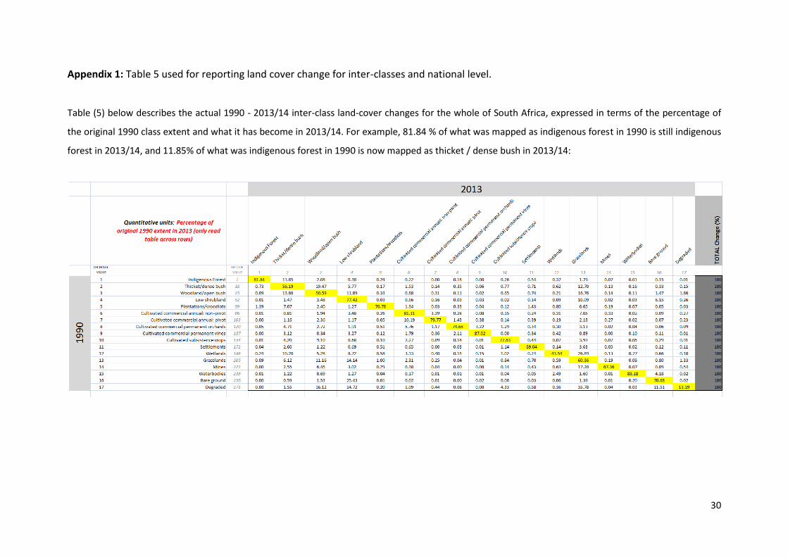
Appendix 1: Table 5 used for reporting land cover change for inter-classes and national level.
Table (5) below describes the actual 1990 - 2013/14 inter-class land-cover changes for the whole of South Africa, expressed in terms of the percentage of
the original 1990 class extent and what it has become in 2013/14. For example, 81.84 % of what was mapped as indigenous forest in 1990 is still indigenous
forest in 2013/14, and 11.85% of what was indigenous forest in 1990 is now mapped as thicket / dense bush in 2013/14:

31
Appendix 2: Outline of variables and parameters for the Bayesian State Space model (BSPM)
framework for GM maize and soybean data analysis.
For each response variable Yi,j,t of crop type i (soy or maize) and metric j (land-use or production) and
province k in year t, an exponential growth model was assumed, such that:
tkjitkjitkji YY ,,,,,,1,,,
Where tji ,, is the growth rate in year t. Growth rate tji ,, was allowed to vary to accommodate
fluctuations in environmental conditions (droughts, rain etc.). State‐space models are hierarchical
models that explicitly decompose an observed time‐series of the observed responses into a process
variation and an observation error component (Simmons et al. 2015). On the log scale, the process
equation becomes (e.g. Simmons et al. 2015)
tkjitkjitkji ,,,,,,1,,, ),0(~ 2
,,, jitji N
where )log( ,,,1,,, tkjitkji Y and )log( ,,,,,, tkjitkji , with variations in log-growth rates realized
as a random normal walk given the estimable process error variance 2
, ji . The observation process
equation was then
tjitjitjiy ,,,,,, )log( ),0(~ 2
,, jiji N
where tjiy ,, denotes the reported values for crop type i for response metric j in province k and year
t, and 2
, ji is the observation variance. For computational reasons, 2
, ji was fixed to 0.12, which
means that a CV ~ 10% was admitted to account for inaccurate reporting in the census data.
Total annual land-use (ha), summed for the whole of South Africa, was then modelled as a function
of:
k
tkjiti YTLU ,,,,ˆ
32
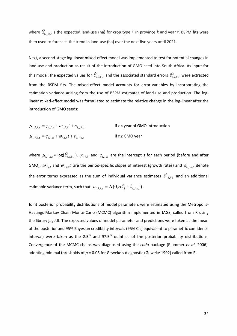
where tkjiY ,,, is the expected land-use (ha) for crop type i in province k and year t. BSPM fits were
then used to forecast the trend in land-use (ha) over the next five years until 2021.
Next, a second-stage log-linear mixed-effect model was implemented to test for potential changes in
land-use and production as result of the introduction of GMO seed into South Africa. As input for
this model, the expected values for tkjiY ,,,ˆ and the associated standard errors 2
,,,ˆ
tkjis were extracted
from the BSPM fits. The mixed-effect model accounts for error-variables by incorporating the
estimation variance arising from the use of BSPM estimates of land-use and production. The log-
linear mixed-effect model was formulated to estimate the relative change in the log-linear after the
introduction of GMO seeds:
tkjikjikjitkji t ,,,,,,,,,, if t < year of GMO introduction
tkjikjikjitkji t ,,,,,,,,,, if t ≥ GMO year
where tkji ,,, = log( tkjiY ,,,ˆ ), kji ,, and kji ,, are the intercept s for each period (before and after
GMO), kji ,, and tkji ,, are the period-specific slopes of interest (growth rates) and tkji ,,, denote
the error terms expressed as the sum of individual variance estimates 2
,,,ˆ
tkjis and an additional
estimable variance term, such that )ˆ,0( ,,,
2
,,,, tkjijitkji sN .
Joint posterior probability distributions of model parameters were estimated using the Metropolis-
Hastings Markov Chain Monte-Carlo (MCMC) algorithm implemented in JAGS, called from R using
the library jagsUI. The expected values of model parameter and predictions were taken as the mean
of the posterior and 95% Bayesian credibility intervals (95% CIs; equivalent to parametric confidence
interval) were taken as the 2.5th and 97.5th quintiles of the posterior probability distributions.
Convergence of the MCMC chains was diagnosed using the coda package (Plummer et al. 2006),
adopting minimal thresholds of p = 0.05 for Geweke’s diagnostic (Geweke 1992) called from R.
33
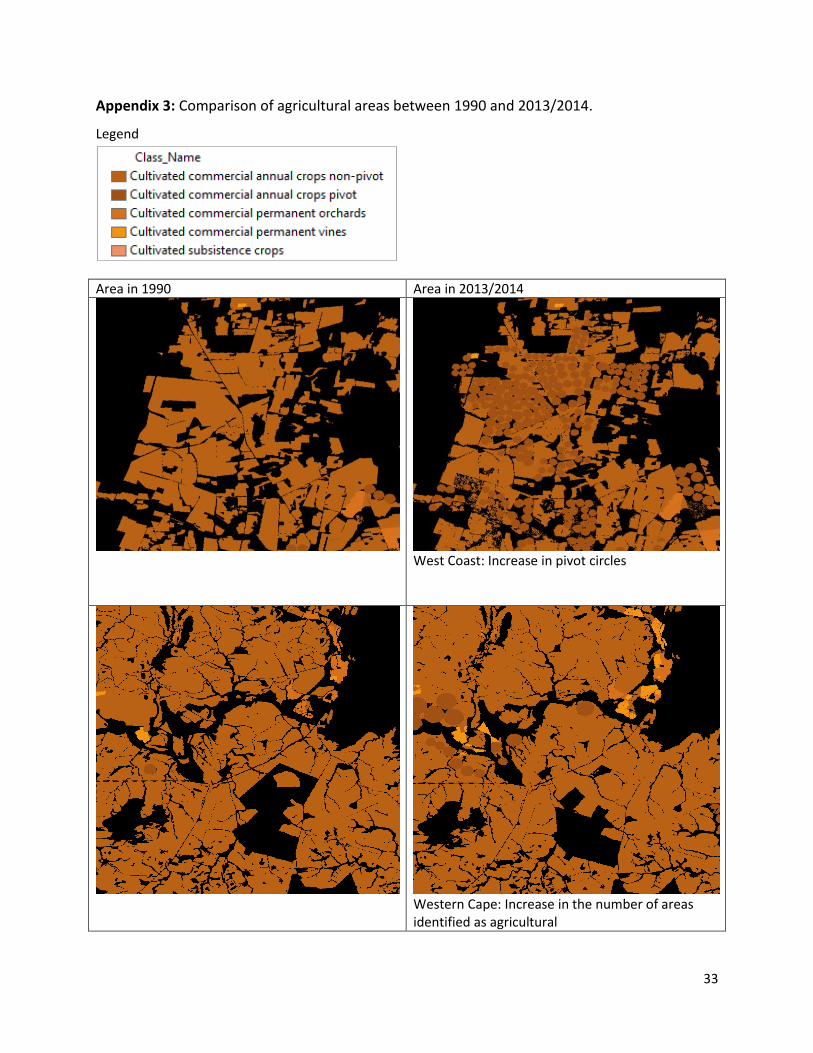
Appendix 3: Comparison of agricultural areas between 1990 and 2013/2014.
Legend
Area in 1990 Area in 2013/2014
West Coast: Increase in pivot circles
Western Cape: Increase in the number of areas identified as agricultural

34
Eastern Cape: Increase in subsistence agriculture
Limpopo: less areas identified as agriculture in 2014
35
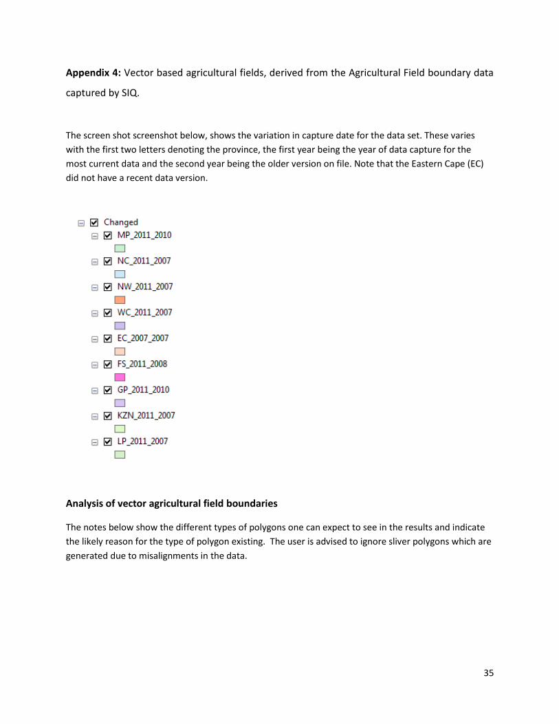
Appendix 4: Vector based agricultural fields, derived from the Agricultural Field boundary data
captured by SIQ.
The screen shot screenshot below, shows the variation in capture date for the data set. These varies
with the first two letters denoting the province, the first year being the year of data capture for the
most current data and the second year being the older version on file. Note that the Eastern Cape (EC)
did not have a recent data version.
Analysis of vector agricultural field boundaries
The notes below show the different types of polygons one can expect to see in the results and indicate
the likely reason for the type of polygon existing. The user is advised to ignore sliver polygons which are
generated due to misalignments in the data.
36
New field
Change in field
boundary –
most likely an
error - ignore
Field removed –
potential
misclassification -
ignore
Old field boundaries - 2007 New field boundaries - 2011

37
New Field
A new field is one that appears in the recent layer, e.g. 2011, but not in the old layer, e.g. 2007
A new field should have been captured recently, check the two dates in the Captured column to confirm
this, for example in the above information Captured shows 2011 and not 2007.
New fields should also have a large area, in most cases the value shown in OArea should Equal the value
shown in NArea (see above), however changes in projections and editing errors can result in area
differences.
Type shows you the type of agriculture practiced in this new field
Removed Fields – Data Error
Removed fields are areas that existed in the old layer, e.g. 2007 and not in the new layer, e.g. 2011. It is
likely that when the new fields were captured an error was noted and corrected, perhaps a dam that
wasn’t seen in the previous imagery. In the above example, OArea is larger than NArea, because this
area was part of a larger field, only a small portion of the 2007 field was removed. The date shown in
Captured is that of the older layer.
Change in field boundary – Data Error
A change in field boundary between the two data layers causes a silver (small polygon) to form. In the
above example you can identify this by the NArea that is significantly smaller than the OArea. The date
in Captured could be either 2007 or 2011.


