
An Implicit Viscosity Formulation for SPH Fluids
Andreas Peer et al.SIGGRAPH 2015
Copyright of figures and other materials in the paper belongs original authors.
Presented by Min-ju Park
2017.02.22
Computer Graphics @ Korea University
Min-ju Park | 2017. 02. 22 | # 2Computer Graphics @ Korea University
Abstract
• We present a novel implicit formulation for highly viscous fluids
• Compare to explicit method
more efficient
handles a larger range of viscosities
• Compare to existing implicit method
our approach reconstructs the velocity field from a target velocity gradient
• encodes a desired shear-rate damping
• preserves the velocity divergence
• ensures that pressure and viscosity computation do not interfere

Min-ju Park | 2017. 02. 22 | # 3Computer Graphics @ Korea University
1 Introduction
• Explicit method
• [Modeling low reynolds number incompressible flows using SPH.] (Morris et al., Journal of computational physics 136 ‘97)
• Implicit method
• [Accurate viscous free surfaces for buckling, coiling, and rotating liquids] (Batty et al., SIGGRAPH ‘08)
competing constraints might be neglected in explicit approach, while in implicit, this issue has to be addressed.
Explicit Implicit
𝑦 𝑡 + Δ𝑡 = 𝑓 𝑦 𝑡 𝑦 𝑡 + Δ𝑡
= 𝑓 𝑦 𝑡 + Δ𝑡 + 𝑔(𝑦 𝑡 )
Small timestep Large timestep

Min-ju Park | 2017. 02. 22 | # 4Computer Graphics @ Korea University
1 Introduction
contribution
• This paper proposes a novel implicit formulation for highly viscous SPH fluids
• that addresses the interference of pressure and viscosity computation
• target velocity gradient encode the desired viscosity and preserves arbitrary velocity divergences
• SPH pressure solver introduce some divergence to the velocity field to counteract density deviations
• e.g. IISPH in [Implicit incompressible SPH] (Ihmsen et al., TVCG ‘14)
• Our formulation preserves density corrections that have been computed in the preceding pressure projection.
• This also means that only one pressure projection step is required
Min-ju Park | 2017. 02. 22 | # 5Computer Graphics @ Korea University
2 Related work
Lagrangian techniques
• [Animating lava flows] (Stora et al., GI ‘99) and [Modeling and rendering viscous liquids] (Steele et al., CASA ‘04)
• these approximation improve the stability of low viscous SPH, but are less efficient for highly viscous fluids
• prone to overshooting
• Use an implicit formulation
• it allows for large timestep, so overshooting cannot occur
• Correctly account for desired velocity divergence
• existing formulation assume a divergence-free velocity field
• Our novel formulation bases on target velocity gradient
• does not interfere with the pressure solver
• dose not require a final pressure solver because it possibly perturbs the result of the viscosity solver

Min-ju Park | 2017. 02. 22 | # 6Computer Graphics @ Korea University
2 Related work
Eulerian techniques
• Many Eulerian approaches require some special treatment of free surface to allow for rotational fluid movement or only work on divergence-free velocity field
• [Accurate viscous free surfaces for buckling, coiling, and rotating liquids] (Batty et al., SIGGRAPH ‘08)
• [Multiple interacting liquids] (Losasso et al., ACM TOG ‘06)
• Our Lagragian approach does not require any special treatment and only work on divergence-free
• compute a desired velocity gradient
• does not affect rotation rate
• preserves divergence

Min-ju Park | 2017. 02. 22 | # 7Computer Graphics @ Korea University
2 Related work
Viscosity in multiphase fluids
• By averaging the viscosity constants, handling the interfaces is done in Lagrangian approaches
• [Particle-based fluid-fluid interaction] (Muller et al., SIGGRAPH ‘05)
• In Eulerian, an method is proposed to extrapolate ghost velocities across the interface to counteract distortions in the velocity gradient caused by variable viscosities
• [Discontinuous fluids] (Hong et al., ACM TOG ‘05)
• Our viscosity formulation is incorporated in [Density contrast SPH interfaces] (Solenthaler et al., SIGGRAPH ‘08)
• It does not impose additional costs for multiple phases with different densities and viscosities.

Min-ju Park | 2017. 02. 22 | # 8Computer Graphics @ Korea University
2 Related work
Fluid-solid blending and viscoelastic fluids
• The Navier-Stokes equations are augmented with a term accounting for elastic forces for SPH
• [A point-based method for animating elastoplastic solids] (Gerszewski et al., SIGGRAPH ‘09)
• Our method relies on the plain Navier-Stokes equations for fluids
• does not account for rigid motion and elasticity
Min-ju Park | 2017. 02. 22 | # 9Computer Graphics @ Korea University
2 Related work
Position-based methods
• Our method is implicit
as we solve a linear system for unknown velocities at next timestep
• Similarity to PBD
[A survey on position-based simulation methods in computer graphics] (Bender et al., CG Forum ’14)
• formulate a set of constraints that should be fulfilled at the next timestep
• employ a non-standard parameter between zero to one
our approach could also be seen as a contribution to the development of PBD from geometric towards physical motivations
• Our formulation imposes velocity constraints to damp shear rates which is the physical effect of shear viscosity.

Min-ju Park | 2017. 02. 22 | # 10Computer Graphics @ Korea University
3 Method
• Based on a desired velocity gradient at the next timestep, we compute momentum-preserving velocities that correspond to the predicted gradient.
predict a velocity gradient
preserves the corrections of density deviations
pressure & viscosity solvers do not interfere
Compute velocity changes due to pressure forces
↓
Viscosity solver computes velocities that account for viscosity
(but do not influence the rate of change of the volume)

Min-ju Park | 2017. 02. 22 | # 11Computer Graphics @ Korea University
3 Method
3.1 Decomposition of the velocity gradient
𝛻𝐯 =1
2𝛻𝐯 − 𝛻𝐯 𝑇 +
1
3𝛻 ∙ 𝐯 𝐈 +
1
2𝛻𝐯 + 𝛻𝐯 𝑇 −
1
3𝛻 ∙ 𝐯 𝐈
= R + V + S
• Spin tensor R
rate of rotation, i.e. vorticity
• Expansion-rate tensor V
density change (that computed by pressure solver)
preserved by viscous solver
• Shear-rate tensor S
rate of shear strain
(1)
Min-ju Park | 2017. 02. 22 | # 12Computer Graphics @ Korea University
3 Method
3.2 Prediction of the velocity gradient
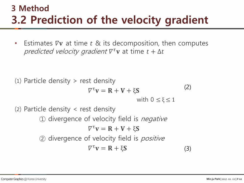
• Estimates 𝛻𝐯 at time 𝑡 & its decomposition, then computes predicted velocity gradient 𝛻𝜏𝐯 at time 𝑡 + ∆𝑡
⑴ Particle density > rest density
𝛻τ𝐯 = 𝐑 + 𝐕 + ξ𝐒
with 0 ≤ ξ ≤ 1
⑵ Particle density < rest density
① divergence of velocity field is negative
𝛻τ𝐯 = 𝐑 + 𝐕 + ξ𝐒
② divergence of velocity field is positive
𝛻τ𝐯 = 𝐑 + ξ𝐒
(2)
(3)

Min-ju Park | 2017. 02. 22 | # 13Computer Graphics @ Korea University
3 Method
3.2 Prediction of the velocity gradient
[Figure 2]
• Estimates 𝛻𝐯 at time 𝑡 & its decomposition, then computes predicted velocity gradient 𝛻𝜏𝐯 at time 𝑡 + ∆𝑡
⑴ Particle density > rest density
𝛻τ𝐯 = 𝐑 + 𝐕 + ξ𝐒
with 0 ≤ ξ ≤ 1
⑵ Particle density < rest density
① divergence of velocity field is negative
𝛻τ𝐯 = 𝐑 + 𝐕 + ξ𝐒
② divergence of velocity field is positive
𝛻τ𝐯 = 𝐑 + ξ𝐒
(2)
(3)

Min-ju Park | 2017. 02. 22 | # 14Computer Graphics @ Korea University
3 Method
3.3 Reconstruction of the velocity field
• Final velocities 𝐯𝑖(𝑡 + ∆𝑡) are reconstructed from𝛻𝜏𝐯𝑖 𝑡 + ∆𝑡
use first-order Taylor approximation
𝐯𝑖 𝑡 + ∆𝑡 = 𝐯𝑗 𝑡 + ∆𝑡 +𝛻𝜏𝐯𝑖 + 𝛻
𝜏𝐯𝑗
2𝐱𝑖𝑗
𝛻𝜏𝐯𝑖+𝛻𝜏𝐯𝑗
2is used to guarantee momentum-preserving velocity
changes at the particles and accounts for the diffusion of the rotation rate
(4)
Min-ju Park | 2017. 02. 22 | # 15Computer Graphics @ Korea University
3 Method
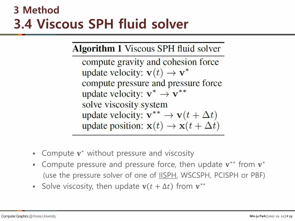
3.4 Viscous SPH fluid solver
Compute 𝐯∗ without pressure and viscosity
Compute pressure and pressure force, then update 𝐯∗∗ from 𝐯∗
(use the pressure solver of one of IISPH, WSCSPH, PCISPH or PBF)
Solve viscosity, then update 𝐯 𝑡 + ∆𝑡 from 𝐯∗∗
Min-ju Park | 2017. 02. 22 | # 16Computer Graphics @ Korea University
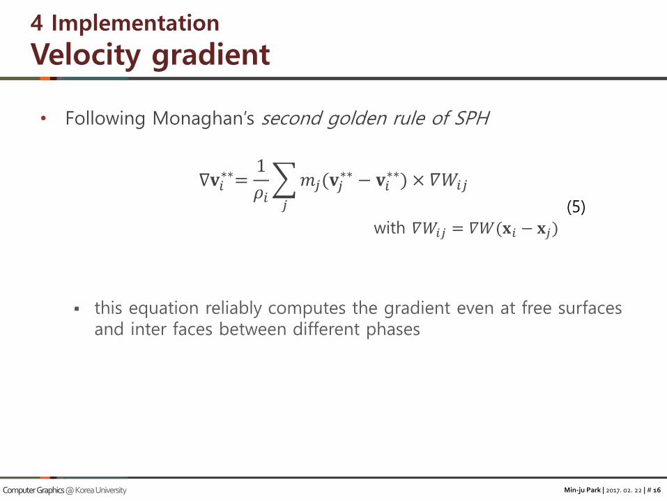
4 Implementation
Velocity gradient
• Following Monaghan’s second golden rule of SPH
∇𝐯𝑖∗∗=1
𝜌𝑖
𝑗
𝑚𝑗(𝐯𝑗∗∗ − 𝐯𝑖
∗∗) × 𝛻𝑊𝑖𝑗
with 𝛻𝑊𝑖𝑗 = 𝛻𝑊(𝐱𝑖 − 𝐱𝑗)
this equation reliably computes the gradient even at free surfaces and inter faces between different phases
(5)
Min-ju Park | 2017. 02. 22 | # 17Computer Graphics @ Korea University
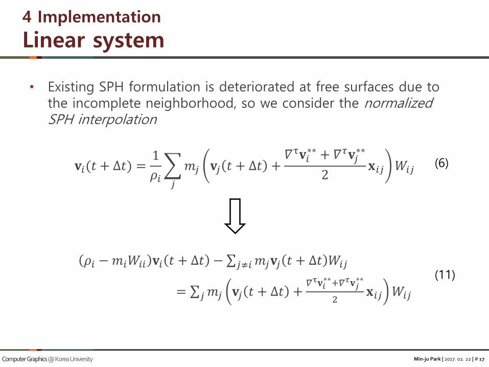
4 Implementation
Linear system
• Existing SPH formulation is deteriorated at free surfaces due to the incomplete neighborhood, so we consider the normalized SPH interpolation
𝐯𝑖(𝑡 + ∆𝑡) =1
𝜌𝑖
𝑗
𝑚𝑗 𝐯𝑗 𝑡 + ∆𝑡 +𝛻τ𝐯𝑖∗∗ + 𝛻𝜏𝐯𝑗
∗∗
2𝐱𝑖𝑗 𝑊𝑖𝑗
𝜌𝑖 −𝑚𝑖𝑊𝑖𝑖 𝐯𝑖 𝑡 + ∆𝑡 − 𝑗≠𝑖𝑚𝑗𝐯𝑗 𝑡 + ∆𝑡 𝑊𝑖𝑗
= 𝑗𝑚𝑗 𝐯𝑗 𝑡 + ∆𝑡 +𝛻τ𝐯𝑖∗∗+𝛻𝜏𝐯𝑗
∗∗
2𝐱𝑖𝑗 𝑊𝑖𝑗
(6)
(11)
Min-ju Park | 2017. 02. 22 | # 18Computer Graphics @ Korea University
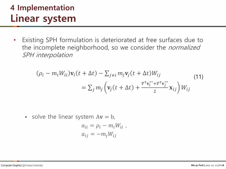
4 Implementation
Linear system
• Existing SPH formulation is deteriorated at free surfaces due to the incomplete neighborhood, so we consider the normalized SPH interpolation
𝜌𝑖 −𝑚𝑖𝑊𝑖𝑖 𝐯𝑖 𝑡 + ∆𝑡 − 𝑗≠𝑖𝑚𝑗𝐯𝑗 𝑡 + ∆𝑡 𝑊𝑖𝑗
= 𝑗𝑚𝑗 𝐯𝑗 𝑡 + ∆𝑡 +𝛻τ𝐯𝑖∗∗+𝛻𝜏𝐯𝑗
∗∗
2𝐱𝑖𝑗 𝑊𝑖𝑗
solve the linear system A𝐯 = b,
𝑎𝑖𝑖 = 𝜌𝑖 −𝑚𝑖𝑊𝑖𝑖 ,
𝑎𝑖𝑗 = −𝑚𝑗𝑊𝑖𝑗
(11)

Min-ju Park | 2017. 02. 22 | # 19Computer Graphics @ Korea University
4 Implementation
Boundary handling
• Sticky boundary
𝐯𝑖 𝑡 + ∆𝑡 =1
𝜌𝑖 𝑗∉𝑏𝑚𝑗 𝐯𝑗 𝑡 + ∆𝑡 +
𝛻τ𝐯𝑖∗∗+𝛻𝜏𝐯𝑗
∗∗
2𝐱𝑖𝑗 𝑊𝑖𝑗
+1
𝜌𝑖 𝑏𝑚𝑏 𝐯𝑏
∗∗𝑊𝑖𝑏
• Separating boundary
𝛻 ∙ 𝐯𝑖𝑙 =
𝑏
𝑚𝑏( 𝐯𝑖𝑙 − 𝐯𝑏
∗∗)𝛻𝑊𝑖𝑏
if this divergence is negative,
𝐯𝑖𝑙 =𝐧𝑖𝐧𝑖 ∙ 𝐧𝑖
𝑏
𝑚𝑏 𝐯𝑏∗∗𝛻𝑊𝑖𝑏
with 𝐧𝑖 = 𝑏𝑚𝑏 𝛻𝑊𝑖𝑏
(12)
(13)
(14)

Min-ju Park | 2017. 02. 22 | # 20Computer Graphics @ Korea University
4 Implementation
Boundary handling
• Sticky boundary use Conjugate gradient method
𝐯𝑖 𝑡 + ∆𝑡 =1
𝜌𝑖 𝑗∉𝑏𝑚𝑗 𝐯𝑗 𝑡 + ∆𝑡 +
𝛻τ𝐯𝑖∗∗+𝛻𝜏𝐯𝑗
∗∗
2𝐱𝑖𝑗 𝑊𝑖𝑗
+1
𝜌𝑖 𝑏𝑚𝑏 𝐯𝑏
∗∗𝑊𝑖𝑏
• Separating boundary use Jacobi method
𝛻 ∙ 𝐯𝑖𝑙 =
𝑏
𝑚𝑏( 𝐯𝑖𝑙 − 𝐯𝑏
∗∗)𝛻𝑊𝑖𝑏
if this divergence is negative,
𝐯𝑖𝑙 =𝐧𝑖𝐧𝑖 ∙ 𝐧𝑖
𝑏
𝑚𝑏 𝐯𝑏∗∗𝛻𝑊𝑖𝑏
with 𝐧𝑖 = 𝑏𝑚𝑏 𝛻𝑊𝑖𝑏
(12)
(13)
(14)

Min-ju Park | 2017. 02. 22 | # 21Computer Graphics @ Korea University
4 Implementation
Multiple phase
• Incorporate the approach of [Density contrast SPH interfaces] (Solenthaler et al., SIGGRAPH ‘08) into IISPH
viscosity system is solved independently for each phase
• Interaction between the phases is accomplished
via pressure and cohesion forces in [Versatile rigid-fluid coupling for incompressible SPH] (Akinci et al., ACM TOG ‘12)

Min-ju Park | 2017. 02. 22 | # 22Computer Graphics @ Korea University
5 Discussion
• Interpretation of the system
1 −𝑚𝑖
𝜌𝑖𝑊𝑖𝑖 𝐯𝑖 𝑡 + ∆𝑡 −
1
𝜌𝑖 𝑗≠𝑖𝑚𝑗𝐯𝑗 𝑡 + ∆𝑡 𝑊𝑖𝑗
=1
𝜌𝑖 𝑗𝑚𝑗 𝐯𝑗 𝑡 + ∆𝑡 +
𝛻τ𝐯𝑖∗∗+𝛻𝜏𝐯𝑗
∗∗
2𝐱𝑖𝑗 𝑊𝑖𝑗
the equation actually estimates velocities that meet an approximated target Laplacian
• it can be interpreted as 𝛻2𝐯𝑖 𝑡 + ∆𝑡 = 𝛻2τ𝐯𝑖∗∗
• Parameter 𝜉
non-standard parameter
dose not correspond to dynamic or kinematic viscosity
governs damping of the shear rate, so governs viscosity
depend on the timestep and resolution
• the time dependency of parameter is not handled as timesteps
(10)

Min-ju Park | 2017. 02. 22 | # 23Computer Graphics @ Korea University
5 Discussion
• Limitations
use various numerical approximation, e.g. SPH approximation and Taylor approximation → results in numerical errors
• But, these errors are small as negligible
should not be used for low viscous fluids such as water
rather expensive for rigid-like materials
• it requires many solver iterations
• viscoelastic model should be preferred

Min-ju Park | 2017. 02. 22 | # 24Computer Graphics @ Korea University
6 Results
• Our viscosity solver is combined with an IISPH pressure solver
cubic spline kernel
• [Smoothed particle hydrodynamics] (Monaghan, REPORTS ON PROGRESS IN PHYSICS 2005)
surface tension
• [Weakly compressible SPH for free surface flows] (Becker et al., ACM SIGGRAPH 2007)
one- or two-way coupled boundary handling
• [Versatile rigid-fluid coupling for incompressible SPH] (Akinci et al.,
CM TOG 2012) and [Boundary handling and adaptive time-stepping for PCISPH] (Ihmsen et al., VRIPHYS 2010)
maximum volume deviation is below 0.1%
• guaranteed by IISPH pressure solver
Min-ju Park | 2017. 02. 22 | # 25Computer Graphics @ Korea University
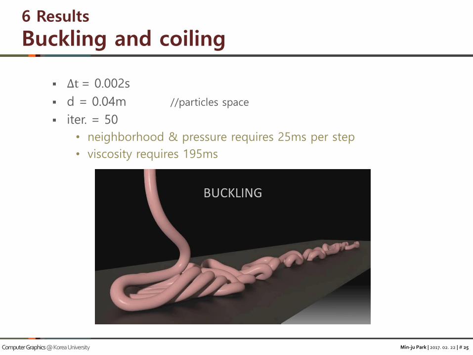
6 Results
Buckling and coiling
∆t = 0.002s
d = 0.04m //particles space
iter. = 50
• neighborhood & pressure requires 25ms per step
• viscosity requires 195ms
Min-ju Park | 2017. 02. 22 | # 26Computer Graphics @ Korea University
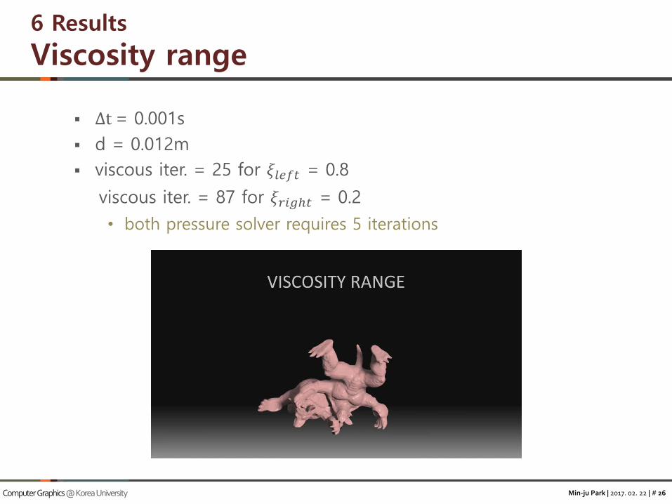
6 Results
Viscosity range
∆t = 0.001s
d = 0.012m
viscous iter. = 25 for 𝜉𝑙𝑒𝑓𝑡 = 0.8
viscous iter. = 87 for 𝜉𝑟𝑖𝑔ℎ𝑡 = 0.2
• both pressure solver requires 5 iterations

Min-ju Park | 2017. 02. 22 | # 27Computer Graphics @ Korea University
6 Results
Rotation rate and density error
∆t = 0.001s
d = 0.02m
𝜉 = 0.5
viscous iter. = 17
pressure iter. = 3
[Figure 6] densities before and after the viscous solve

Min-ju Park | 2017. 02. 22 | # 28Computer Graphics @ Korea University
6 Results
Time-varying viscosity
∆t = 0.001s
d = 0.02m
𝜉𝑏 = 0, 𝜉𝑦 and 𝜉𝑟 = raise form 0 to 0.99 within 3s and 15s
Min-ju Park | 2017. 02. 22 | # 29Computer Graphics @ Korea University
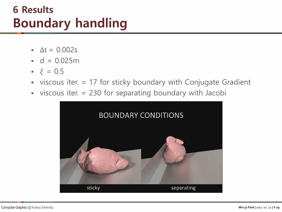
6 Results
Boundary handling
∆t = 0.002s
d = 0.025m
𝜉 = 0.5
viscous iter. = 17 for sticky boundary with Conjugate Gradient
viscous iter. = 230 for separating boundary with Jacobi

Min-ju Park | 2017. 02. 22 | # 30Computer Graphics @ Korea University
6 Results
Complex boundaries
∆t = 0.0004s
d = 0.02m
𝜉 = 0.5
viscous iter. = 12
Min-ju Park | 2017. 02. 22 | # 31Computer Graphics @ Korea University
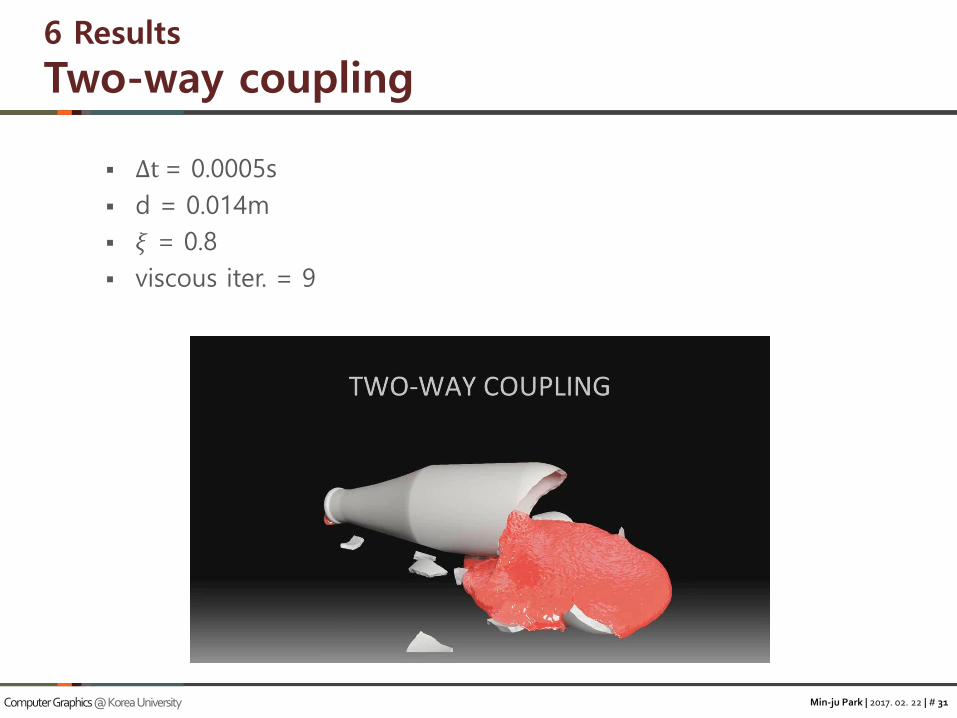
6 Results
Two-way coupling
∆t = 0.0005s
d = 0.014m
𝜉 = 0.8
viscous iter. = 9
Min-ju Park | 2017. 02. 22 | # 32Computer Graphics @ Korea University
6 Results
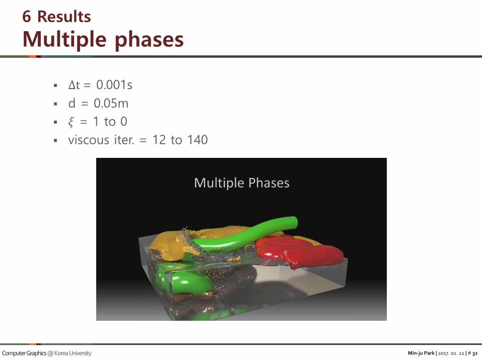
Multiple phases
∆t = 0.001s
d = 0.05m
𝜉 = 1 to 0
viscous iter. = 12 to 140
Min-ju Park | 2017. 02. 22 | # 33Computer Graphics @ Korea University
6 Results
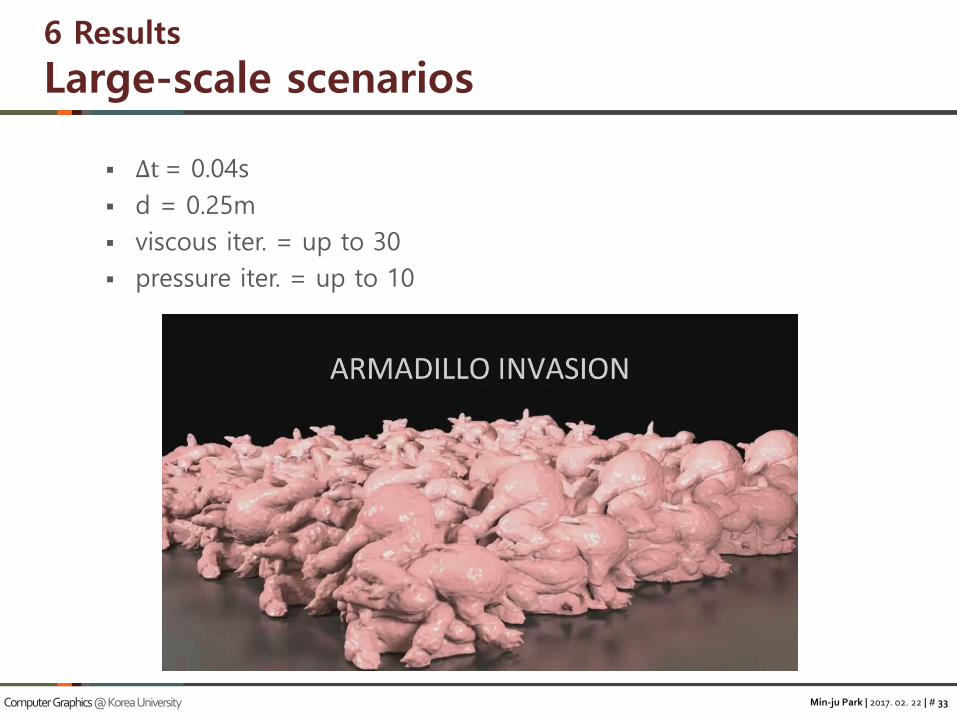
Large-scale scenarios
∆t = 0.04s
d = 0.25m
viscous iter. = up to 30
pressure iter. = up to 10

Min-ju Park | 2017. 02. 22 | # 34Computer Graphics @ Korea University
6 Results
Explicit and implicit viscosity solvers
• Comparison of explicit and implicit
(left) use explicit method in [On the problem of penetration in particle methods] (Monaghan, Journal of Computational physics 82 ‘89)
(right) our implicit method
• explicit required 20min, while implicit required only 11sec
• explicit use the timestep of 0.00002s, but implicit 0.01s
[Figure 12]
Min-ju Park | 2017. 02. 22 | # 35Computer Graphics @ Korea University
6 Results
Explicit and implicit viscosity solvers
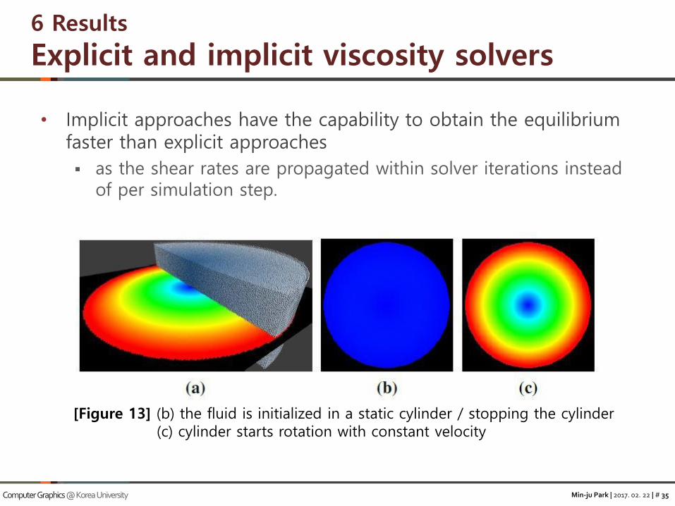
• Implicit approaches have the capability to obtain the equilibrium faster than explicit approaches
as the shear rates are propagated within solver iterations instead of per simulation step.
[Figure 13] (b) the fluid is initialized in a static cylinder / stopping the cylinder(c) cylinder starts rotation with constant velocity
Min-ju Park | 2017. 02. 22 | # 36Computer Graphics @ Korea University
6 Results
Explicit and implicit viscosity solvers
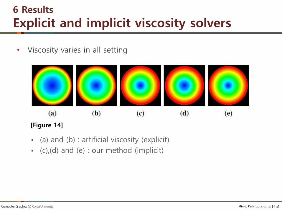
• Viscosity varies in all setting
(a) and (b) : artificial viscosity (explicit)
(c),(d) and (e) : our method (implicit)
[Figure 14]
Min-ju Park | 2017. 02. 22 | # 37Computer Graphics @ Korea University
7 Conclusion and future work
• Our viscosity formulation preserves the density correction
this is achieved by decomposing the gradient
• By integrating our formulation into IISPH
a maximum volume deviation can be guaranteed independent from the grade of viscosity
• More efficient than explicit method
work well with large timestep
versatile in wide range of viscous material
work well in one-/two-way coupling and multiphase simulation
Min-ju Park | 2017. 02. 22 | # 38Computer Graphics @ Korea University
7 Conclusion and future work
• Our method heavily damps shear rates
particle movement is strongly restricted
after simulation, the pattern of initial particle sampling is visible
• it is problematic for regular sampling patterns
• Conjugate gradient method does not work in separating boundary
in separating boundary, intermediate results have to be adjusted in each solver iteration


