An Investigation into the System Production
Balance within Three Mechanised
Harvesting Case Studies
A dissertation submitted in partial fulfilment of the requirements for
the degree of Bachelor of Forestry Science with Honours by:
K. K. Malietoa
New Zealand School of Forestry
University of Canterbury
Christchurch
New Zealand
2016

i
1.0 Abstract
Safety issues and high costs of traditional harvesting methods have been driving
mechanisation increases in New Zealand. However, productivity increases from
mechanisation alters system productivity balance. This can result in underutilised
machinery and cause an increase in harvesting costs in real terms.
A time study was carried out to understand the system productivity balance between
felling, extraction and processing and the factors affecting system component productivity
rates, for three case studies. The three case studies observed were (1) a semi-mechanised
cable yarder extraction operation, (2) a fully-mechanised swing yarder operation and (3) a
fully-mechanised ground based operation.
There were large production imbalances between felling, extraction and processing in all
three case studies. Felling was the most productive system component, being 98%, 37%
and 88% (case studies 1 to 3 respectively) more productive than the bottleneck. System
bottleneck for case studies 1 and 3 was extraction, and processing for case study 2.
The number of stems bunched, number of stems shovelled, wind throw interference and
machine position shift affected felling cycle time. For every stem bunched, average
productivity decreased by 35% (24m3/PMH) and 21% (20.9m3/PMH) for case studies 2
and 3 respectively. Every additional stem shovelled reduced felling productivity by
7.4m3/PMH for case study 2. Haul distance, the number of stems extracted and site factor
affected extraction productivity. Haul distance and the number of stems extracted had
significant impact on hourly productivity for all case studies. Site factor affected hourly
productivity by 6.9m3 and 56.7m3 for case studies 1 and 3 respectively, largely attributed
to the cable system employed and ground conditions. Processing was affected by the
number of logs cut per stem and if delimbing occurred. Delimbing and each additional log
processed, decreased productivity by 16% and 14% respectively.
These three case studies showed that mechanised systems are often not well balanced and
result in system components being underutilised. Companies can consider task strategies,
or machine sharing between systems to minimise the effect on cost.
Key Words: Mechanised Harvesting, Production Balance, Operational Efficiency,
Productivity, Utilisation, Forestry.

ii
2.0 Acknowledgements
Firstly I would like to thank my project supervisor Rien Visser and additional help from
Hunter Harill, for the guidance I received and the time taken out of his schedule to assist
with the project.
I would like to thank the team at Nelson Management Ltd for providing the project
opportunity as well as staff knowledge and utilities to complete the project. In particular
David Robinson for setting up the project and providing guidance essential in completing
the project. I would also like to thank Nathan Sturrock for aiding me with the project
through collection of machine data.
I would also like to acknowledge harvesting crews Bryan Heslop Logging, Endurance
Logging and Fraser Logging for allowing data collection of their operations and assistance
with the time and motion study.
Lastly, I would like to thank and acknowledge my parents Tanu and Kaylene for their
support and encouragement throughout the year and the rest of the BForSc class for
supporting and driving one another to complete our projects and the enjoyable times spent
together during this time.
iii
Table of Contents
1.0 Abstract ............................................................................................................................. i
2.0 Acknowledgements ......................................................................................................... ii
Table of Contents ................................................................................................................. iii
3.0 Introduction ..................................................................................................................... 1
3.1 Background .................................................................................................................. 1
3.2 Problem Statement ....................................................................................................... 2
4.0 Literature Review ............................................................................................................ 3
4.1 Study Method ............................................................................................................... 3
4.2 System Production Balance in Harvesting Operations ................................................ 4
4.3 Mechanisation Cost and System Production Balance .................................................. 4
4.4 Mechanisation in New Zealand and System Production Balance ............................... 5
4.5 Previous Studies ........................................................................................................... 6
5.0 Method ............................................................................................................................. 8
5.1 Study Location ............................................................................................................. 8
5.2 Case Study Description ................................................................................................ 9
5.2.1 Case Study 1: Semi-Mechanised Tall Tower Operation ....................................... 9
5.2.2 Case Study 2: Fully-Mechanised Swing Yarder Operation ................................ 10
5.2.3 Case Study 3: Fully-Mechanised Ground Based Operation................................ 11
5.2.3 Data Collection ....................................................................................................... 11
5.2.5 Data Analysis .......................................................................................................... 13
5.2.5.1 Multiple Linear Regression .............................................................................. 13
5.2.5.2 Multiple Linear Regression .............................................................................. 14
5.2.5.3 One-Way ANOVA ........................................................................................... 14
6.0 Results ........................................................................................................................... 15
6.1 Operational Phase Statistics ....................................................................................... 15
6.1.1 Felling Operational Phase Statistics .................................................................... 15
6.1.2 Extraction Operational Phase Statistics............................................................... 16
6.1.3 Processing Operational Phase Statistics .............................................................. 17
6.2 System Production Balance ....................................................................................... 18
6.3 Cycle Time Analysis .................................................................................................. 19
6.3.1 Felling Cycle Time Analysis ............................................................................... 19
6.3.2 Extraction Cycle Time Analysis ......................................................................... 21
6.3.3 Processing Cycle Time Analysis ......................................................................... 26
6.4 Productivity Analysis ................................................................................................. 28

iv
7.0 Discussion ...................................................................................................................... 30
7.1 System Production Balance ....................................................................................... 30
7.2 Factors affecting Felling ............................................................................................ 30
7.3 Factors affecting Extraction ....................................................................................... 31
7.4 Factors affecting Processing ...................................................................................... 33
7.5 Further Analysis ......................................................................................................... 33
7.5 Limitations ................................................................................................................. 34
8.0 Conclusion ..................................................................................................................... 36
9.0 References ..................................................................................................................... 37
10.0 Appendix ..................................................................................................................... 39
10.1 Study Location Slope Maps ..................................................................................... 39
10.2 Regression Outputs .................................................................................................. 42

1
3.0 Introduction
3.1 Background
New Zealand forest harvesting on steep terrain has numerous safety issues with traditional
methods used. Traditional methods are motor-manual felling followed by cable extraction
with choker-setters (colloquially called breaker-outs in New Zealand) and motor-manual
processing at the landing (Visser, Raymond & Harill, 2014a). 2008 to 2013 witnessed
thirty-two forestry fatalities making it New Zealand’s most dangerous industry (Adams,
Armstrong & Cosman, 2014), with the highest reported incident rates within harvesting
operations (Bentley, Parker, & Ashby, 2004). 5 forestry fatalities have occurred to date in
2016 (September), 4 of which from traditional methods (2 manual felling, 2 breaking-out).
The dangerous working environment has resulted in a poor safety record for traditional
harvesting methods. There are doubts that such hazards can be permanently removed from
the workplace (Adams et al., 2014; Amishev, 2012).
Traditional methods are also associated with harvesting high costs due to a combination of
low production operations and operating costs. Highly productive, fully-mechanised
ground based operations, are at least 50% cheaper than cable extraction operations
employing traditional methods (Raymond, 2012). The low profit margin associated with
steep terrain harvesting requires more cost effective harvesting methods for the New
Zealand forest industry to remain internationally competitive and continue future growth
(Raymond, 2012).
With the area of steep terrain harvesting to increase to 77% by 2030 (Raymond, 2012), the
issue of safety and high harvesting costs on steep terrain is increasing in importance. A
long term solution to ensure a safer working environment, at lower unit cost is exchanging
traditional methods with machinery (called mechanisation). On flat terrain the transition
has been straight forward through introductions of felling machines, skidders and
forwarders, and mechanised processors (Amishev, 2012). Difficulty arises on slopes
greater than 27 degrees with ground based felling and extraction methods deemed
unsuitable (Amishev, 2012). In recent years a strong industry drive has seen a focus
towards more mechanised operations, to achieve greater safety and cost-effectiveness on

2
steep terrain (Visser, Raymond & Harrill, 2014b). Most recent developments include a
range of cable assist felling systems and innovative motorized grapple carriages.
3.2 Problem Statement
Nelson Forest Limited (NFL) have worked alongside industry objectives to increase safety
and reduce harvesting costs on steeper terrain through mechanisation. Numerous cable
contractors have introduced tethered falling machines, complementing mechanised
extraction and processing components. Capability of ground based operations have been
pushed onto steeper terrain to reduce harvesting costs. Certain ground based operations
include self-levelling felling machines with tether ability extending felling and shovelling
capability.
Through increased levels of mechanisation, the consideration of wood flow within an
operation is vital. In any harvest system, individual operational phases aim for balanced
production with the preceding and/or following phase. Uneven balances of productivity
causes utilisation levels to drop, resulting in increased harvesting costs in real terms
(Competenz, 2005).
Additionally increasing mechanisation results in greater operational costs. With the already
tight profit margin of harvesting on steep terrain, increased machinery costs and likely to
fall NZ dollar (driving up already inflated machine costs), profitability on steep terrain
becomes progressively more sensitive with increasing mechanisation (Raymond, 2012).
The effect of uneven production balance within mechanised harvesting systems has been
identified by NFL as an area of improvement to reduce harvesting costs on steeper terrain.
The major objectives of this study are to:
Understand the system productivity balance between felling, extraction and
processing system components for three case studies.
Determine the major factors affecting productivity of each system component (e.g.
haul distance, piece size) and how understanding these factors can be used to
achieve more balanced systems.

3
4.0 Literature Review
4.1 Study Method
Studies of forestry operations are often difficult and challenging due to the range of
variability associated with activities. Productivity studies require a time consumption to be
associated with some sort of product output (Acuna et al., 2011). In harvesting operations
log/tree production is measured by the amount of time input to calculate productivity.
The most common methods for collecting productivity data are detailed time and motion
studies and shift-level studies (Olsen, Hassain, & Miller, 1998). Aim of time studies are to
analyse time inputs in order to relate them to operational variables or work conditions, with
a typical purpose to analyse operational efficiency (Musat et al., 2015). Time and Motion
studies are suited to short term applications, providing a snapshot of the observed operation
and consequently have limited value in estimating long-term trends (Olsen et al., 1998).
Shift level studies occur over a longer study period, capturing a range of conditions, with
limited operational detail.
Time and Motion studies have the benefit of high precision (down to 1 second) through
splitting studies into cycles and associated work elements. This allows work processes to
be described in greater detail and provide greater understanding of system dynamics
(Acuna et al., 2011). Greater description of the system dynamics can benefit through
identifying specific machine element times, delineating productive time from delay time
and separating elements that react differently to work factors (Acuna et al., 2011).
Studies have become increasingly difficult with the increase of mechanised operations.
When conducting time studies on mechanised operations, the duration of work elements
can be short with difficulty separating element changes (Musat el al., 2015). The diversity
of felling machines also increases study difficulty with greater variability and uncertainty
of activities completed (Acuna et al. 2011).

4
4.2 System Production Balance in Harvesting Operations
In all harvesting operations, system balance is aimed to be achieved for all system
components in order to achieve operational efficiency (Competenz, 2005). Operational
efficiency is defined as the ratio of productive time to scheduled time. Control of
downtime and system component productivity within an operation is required to achieve
operational efficiency (Smidt, Tufts, & Gallagher, 2009).
The aim of balanced systems is to achieve even wood flow through all system components,
with the reduction of major bottlenecks to the greatest degree possible. The bottleneck
(limiting productive phase) restricts operation production and causes disruptions between
system components through interference (Competenz, 2005). More productive machinery
become underutilised, reducing the ratio of productive time to scheduled time (i.e. reduced
utilisation). Utilisation of forestry machinery significantly impacts harvesting costs and is
one of the most important factors influencing machine rate calculations (Holzleitner,
Stampfer, & Visser, 2011).
The complexity of harvesting operations influences machine productivity rates within an
operation, affecting system production balance and operational efficiency. The issue is that
many of the factors influencing productivity and efficiency are out of the contractor’s
control (Smidt et al., 2009). Contractors and forest managers look to alleviate effects of
influential factors through alterations of harvesting systems and techniques employed
(Smidt et al., 2009). Understanding of such factors can support strategic and operational
planning within an operation (Holzleitner, Stampfer, & Visser, 2011), which can balance
system productivity and positively influence machine utilisation.
4.3 Mechanisation Cost and System Production Balance
Logging machines are extremely expensive (Riddle, 1995). Increasing mechanisation
within an operation significantly increases overall system costs, which are aimed to be
offset through production benefits. As an example, the ClimbMax steep slope felling
machine is estimated to cost $1750 per day (based on 8 PMH) (Amishev & Evanson, 2013)
in comparison to a manual faller rate that mainly comprises of labour costs. Approximately
half of the machine rate in operations can be attributed with owning costs (driven by

5
capital costs, resale and machine life) (Raymond, 2012). The ClimbMax felling machine
has an estimated capital value (base machine and modifications) of $1,030,000 (Amishev
& Evanson, 2013) in comparison to a new Stihl 660 magnum chainsaw valued at $3295
(Stihl Shop, 2016). Machine owning costs occur whether the machine is working or not.
When machinery are underutilised, machine owning costs continue to be incurred,
increasing logging costs in real terms (Competenz, 2005). An example of an imbalanced
mechanised system stated balancing of the system could reduce production cost by 59
percent (Pan et al, 2008) (this study however did not take into account all operational
costs). Increasing efficiency is therefore needed to compensate for the steadily rising cost
of equipment (Pfeiffer, 1967).
4.4 Mechanisation in New Zealand and System Production Balance
Purpose built, self-levelling felling machines began the shift towards mechanised felling on
steeper terrain 20 years ago (Raymond, 2012). Recent innovation has come from cable-
assist felling machines, revolutionising steep terrain felling in New Zealand. Cable assist
systems were introduced to increase the range ground based machinery, either for felling
and bunching in a cable logging operations, or felling and shovelling in ground based
operations (Visser, Raymond & Harill, 2014). New Zealand’s first example of cable assist
technology occurred in 2007 with a Nelson contractor, attaching a cable-winch to an
excavator to bunch and shovel stems, aiding yarder extraction (Evanson & Amishev,
2010). Numerous tethered felling systems have transpired from the introductory cable
assist machine, such as the Falcon Winch Assist system and ClimbMax steep slope falling
machine.
Traditional methods of manual breaking-out remain the most common cable extraction
method employed, with limited mechanisation shifts in cable yarding over the past 35
years (Raymond, 2012). The major piece of innovation with cable yarding was the
introduction and development of swing yarders in 1987 (Raymond, 2012). Recent
innovation has occurred through mechanised grapple carriages for tower yarders such as
the Falcon Forestry Claw and Alpine Logging Grapple, aimed at reducing accumulation
time of the cycle. Mechanised grapple carriages, although becoming more widespread
were used by less than 25% of a recent survey during a five year period (Harrill and Visser,
2011).

6
Despite less than half of operations utilising mechanised processing, log processing has
seen the greatest degree of innovation over the past 25 years (Raymond, 2012). The major
shift within New Zealand harvesting operations has been the introduction of Waratah’s
single-grip, processing head. The Waratah processing head has been designed and
manufactured specifically to process New Zealand’s radiata pine (Saathof, 2014).
Increased mechanisation aimed at increasing production has affected the system
productivity balance within harvesting operations. Intuitively contractors attempt to reduce
unit costs as much as possible by utilising machinery to their full capacity (Riddle, 1995).
Higher production of mechanised systems have frequent production imbalances between
system components felling, extraction and processing (Evanson & Amishev, 2010).
Unbalanced systems require varying work hours per system component to balance
production, with more productive machinery typically underutilised. Motor manual
systems have the luxury of shifting workers between activities to balance system
productivity, however this is much more difficult and problematic with machinery (Riddle,
1995).
4.5 Previous Studies
Limited studies have occurred observing the production balance between felling,
harvesting and processing of mechanised systems (including tethered felling machines) on
steeper terrain. Typical studies observe a single system component with fewer studies
observing how system components production rates compare within an operation. 2 New
Zealand studies of fully mechanised, swing yarder operation have been observed to analyse
the production balance within the system. Bunched yarder extraction was the most
productive (74.1m3/PMH) in the first study, following by felling (64.7m3/PMH),
processing (57.7m3/PMH) and unbunched extraction as the operational bottleneck at
48.8m3/PMH (Evanson & Amishev, 2010).
An alternate study identified processing as the most productive operational at
86.0m3/PMH. Extraction was the operational bottleneck at 62.6m3/PMH, with felling
average hourly productivity at 80.5m3/PMH (Eavnson & Amishev, 2009).

7
Many studies have been conducted over the years to evaluate factors that affect production
of harvesting operations. Principle factors influencing operation and equipment
productivity are well known from studies conducted over the years (Gardner, 1980).
Depending on site and operation structure, factors affecting machine productivity will
vary. Examples of factors that are commonly found to have effect on productivity include
yarding distance, terrain and slope, number of logs extracted and piece size (Gardner,
1980).

8
5.0 Method
5.1 Study Location
The study observed three harvesting operations within the NFL estate throughout Nelson
and Marlborough. Six sites were studied with each operation observed at 2 sites. Three
sites were studied during summer and three sites during winter. Sites were chosen based on
the location of the harvesting operation at time of data collection. Stand and Slope maps
for each study sites including haul corridors are included in the Appendix for additional
site information. Stand characteristics for each block are summarised below:
Table 1: Stand Characteristics of the 6 study sites
Block Crop Stocking
(SPH)
Merchantable
Piece size
(m3)
Average
Slope (0)
Max Slope
(0)
Western
Boundary, Golden
Downs
PRAD
1990
469 1.23 28.7 40.7
Long Gully,
Golden Downs
PRAD
1990
218 1.6 26.2 34.3
Brightwater Block PRAD
1987
218 2.5 25.1 34.2
Olivers, Golden
Downs
PRAD
1989
331 1.47 22.1 28.8
Pascoes, Golden
Downs
PRAD
1988
284 2.3 12.8 24.8
Fairacres, Wairau
South
PRAD
1988
256 1.64 26.6 34.9

9
5.2 Case Study Description
5.2.1 Case Study 1: Semi-Mechanised Tall Tower Operation
Table 2: System Component, Machine Description and Site for Case Study 1
System Component Machine Description Site
1. Felling Tigercat 655, tethered Self-
levelling felling machine.
Western Boundary, Golden
Downs.
2. Extraction Washington 127 – Manual
B/O, Shotgun system.
Western Boundary, Golden
Downs.
2. Extraction Washington 127 – Manual
B/O, Running skyline
system.
Long Gully, Golden
Downs.
3. Processing Tigercat excavator &
Waratah Processing head.
Western Boundary, Golden
Downs.
During the study operation, the felling machine was secured to a winch assist excavator
operating mid-upper slope of a long face. The winch assist machine, situated at the top of
the slope provided power to aid movement of the felling machine. The operating method
was to fell trees into the stand or parallel to the stand edge. Bunching occurred by rotating
stems into bunches above the cutover. Multiple stems were often felled followed by
bunching perpendicular to direction of the slope.
The yarder used for extraction was a Washington 127 with manual choker-setters. Live
skyline with shotgun carriage and scab (grabinski) systems were used at the Western
Boundary (site 1) and Long Gully (site 2) respectively. At Western Boundary a large patch
of ‘dead ground’ (previously extracted cutover) of around 150 metres was yarded across.
Stems were unhooked by a pole man at the landing and cleared by the Tigercat processing
machine. Trees were delimbed and processed during chute clearance away from the yarder,
above the stand.

10
5.2.2 Case Study 2: Fully-Mechanised Swing Yarder Operation
Table 3: System Component, Machine Description and Site for Case Study 2
System Component Machine Description Site
1. Felling Sumitomo tethered felling
machine, Satco felling head.
Brightwater Block, Golden
Downs
2. Extraction Madill 122 swing yarder,
grapple extraction.
Brightwater Block, Golden
Downs
2. Extraction Madill 122 swing yarder,
grapple extraction.
Olivers rd, Golden Downs
3. Processing Sumitomo Excavator,
Waratah processing head.
Brightwater Block, Golden
Downs
Felling was completed by a Sumitomo excavator with a fell and bunch head. The tethered
felling machine was secured by a cable assist excavator at the top of the slope. Felling of
stems occurred while working up and down the felling face. The operating method was to
fell multiple stems downhill followed by shovelling.
Extraction was completed by a Swing Yarder with mechanical grapple on a running
skyline system. An excavator with raised T-bar was used for the functions of a tail hold.
Stems were either grappled from the deck (bunches) or fed into the grapple by an
excavator (also used to shovel and bunch stems to haul corridors). Logs were extracted to a
small landing and cleared by either the processor (Olivers block) or excavator for two
staging by grapple skidder (Brightwater block).
Processing was completed by a Sumitomo excavator attached with a Waratah processing
head. The processor works in a circular motion, choosing stems from a surge pile created
from the two-stage operation. Stems were completely delimbed at the edge of the skid
prior to log processing.

11
5.2.3 Case Study 3: Fully-Mechanised Ground Based Operation
Table 4: System Component, Machine Description and Site for Case Study 3
System Component Machine Description Site
1. Felling Tigercat 655, tethered Self-
levelling felling machine.
Pascoes Block, Golden
Downs
2. Extraction
Cat 535 Grapple Skidder Pascoes Block, Golden
Downs
2. Extraction
Cat 535 Grapple Skidder Fairacres Block, Wairau
South
3. Processing Cat Excavator & Waratah
Processor
Pascoes Block, Golden
Downs
During the study operation of Case Study 3, felling and delimbing was completed by a
self-levelling John Deere felling machine. Felling occurred on rolling country with patches
of wind throw scattered throughout the stand. The operating method of the felling machine
was to fell trees into or parallel to the stand. The felled stem was then slewed away from
the stand where delimbing occurred prior to being released in a butt first orientation.
The first stage of extraction is completed by a shovelling excavator. Stems are shovelled
from the cutover into bunches at trails for skidder extraction. The operating method for the
skidder extraction was to drive uphill along the skidder trail to stems and extract drags
downhill to the landing, prior to dropping stems in a surge pile. Processing is completed
by a CAT excavator attached with a Waratah processing head. Stems are picked up by the
processing head at the butt end and processed into logs. Stems rarely requiring delimbing
(roughly 10% of the time) due to field delimbing by the felling machine.
5.2.3 Data Collection
A detailed time and motion study was used to capture data for each of the system
components studied. The ‘time study’ application created by NuVizz was used to capture
data of work cycles and corresponding cycle elements. The total study time for each
system component ranged between 5.5 and 12 hours. Longer studies were spent with
extraction operations to gather a sufficient number of cycles for analysis. Factors
corresponding with cycle elements were captured, such as haul distance and stem
extraction. Binary factors measured throughout data collection were listed as 1 or 0
depending on occurrence throughout cycle (1 = factor occurred during observed cycle, 0 =

12
factor did not occur). System component cycle elements and corresponding definitions
(including elements specific to single Case Studies) are listed below:
Felling Cycle Elements
Shift - Machine shifts position and attaches to next standing tree.
Fell - Felling head (attached to tree) cuts tree to the deck.
Bunch - Felled stem are slewed and repositioned into bunches away from the stand.
Shovel - Stem is shovelled away from the felled location.
Delimb – felling head delimbs stem from butt to head with 1 pass of the stem.
Extraction Cycle Elements
Outhaul - Machine/carriage begins to move from landing to stand and stops/slows
significantly above drag.
Hookup - Grapple/carriage accumulates payload (which includes lowering and
raising grapple/carriage) to the point that it begins towards the landing.
Inhaul - Drag begin moves until it stops at the landing.
Unhook - Stems are shovelled away from the felled location.
Processing Cycle Elements
Slew – Machine slews and grabs next stem after previous log has been cut.
Delimb – The stem is pushed through processing head from butt end to head and
back, removing limbs.
Processing - Stems are processed into logs following delimbing.
Whenever the machine was not productive (performing a common element) this was
classed as a delay. Common delays for all system components were classified as the
following:
Delay Elements
Mechanical - Delay caused by mechanical issues/breakdown occurred to the
machine.

13
Operational - Delay that is required for operations to occur, however is not part of
the typical work cycle.
Other - Any other delay that could occur.
A laser range finder was used to determine distance of the carriage or grapple along the
haul corridor. As it was unsafe to be situated near the yarder and tail hold of the cable
operations, trigonometry equations were used to calculate accurate haul distance. Ground
based haul distance was calculated using a mixture of scale forest maps and laser range
finder measurements.
Throughout the time study of each system component, a number of additional factors were
measured that were associated with the operation, for example, shovel fed hook up,
extraction distance and logs cut per stem. Additional factors were measured through direct
observation of the system component. Factors that were unable to be effectively
quantitatively measured were noted as a binary variable (i.e. factor occurred or did not
during the productive cycle). Examples of binary variables used were wind throw and
shifting position between standing trees for the felling operation.
5.2.5 Data Analysis
5.2.5.1 Multiple Linear Regression
To calculate the underlying productivity balance within each of the case studies, individual
system component productivity rates were required. Delay free productivity rates for each
system component were calculated and compared with other system components (within
individual operations) to identify the system productivity balance. Insufficient samples of
delays were observed throughout the study and resultantly not included in analyses.
For each system component, summary statistics were gathered for average cycle elements,
cycle times and productivity rates. Element and cycle information provided information
necessary for machine productivity calculations. Cycle element statistics provide
information and identification of variability within particular elements, allowing areas of
identification for further study and aid understanding factors affecting productivity.

14
5.2.5.2 Multiple Linear Regression
To identify factors that significantly affect cycle time and productivity for each of the
system components, multiple linear regression was used. Multiple linear regression was
used as a substitute of stepwise linear regression due to the limited number of factors
observed. Comparison of influential factors was completed in Microsoft Excel under the
Data Analysis toolbar, providing regression coefficients, standard errors, t value, p value
and standardised estimates (shown in Appendix tables). The statistical significance of
measured variables was based on an alpha (significance level) of 0.05. A significance level
of 0.05 was applied to the regression analysis due to the conventional use of this value in
statistical studies (Perneger, 1998). The typical significance level applied in forest
operations is 0.1 due to the variability observed in operations, however this alpha will
detect a wider range of difference that may occur. Numerous regressions were run to
analyse the effect of observed factors for each system component within each case study.
Similarity of processing operations on the landing allowed for a single regression to be for
this system component across case studies. Regression outputs of individual system
components were included in the Appendix.
5.2.5.3 One-Way ANOVA
Throughout the analysis, certain variables will likely be not significant in predicting cycle
time or productivity, however field observations and logic would suggest a significant
impact. To test the effect of certain factors on individual elements or productivity further
analysis was conducted to test significance through a one-way ANOVA. The one-way
ANOVA test allowed comparison the means to analyse if they were significantly different
from one another.
One-Way ANOVA test was completed using the Data Analysis toolbar in Microsoft Excel.
A significance value of 0.05 was used to determine if the mean values were significantly
different. The One-Way ANOVA is appropriate for this additional analysis as only two
groups of means were compared. Greater quantities of means require an ‘omnibus’ test to
evaluate which specific groups were significantly different from one another.

15
6.0 Results
6.1 Operational Phase Statistics
6.1.1 Felling Operational Phase Statistics
Table 5: Felling cycle and productivity statistics for the three case studies observed.
During observations of case study 1, 204 felling cycles were completed at an average cycle
time of 82.8 seconds or 1.38 minutes. Throughout the study work elements were often
completed in a random order (cycle defined by tree felled) due to operator preference and
site conditions. Elements, bunching and slash clearance only occurred within 69 and 49
respectively of the observed cycles. With an average stand piece size of 1.6 tonne, delay
free productivity (per PMH) was calculated at 69.6m3/PMH from 43.5 trees felled/PMH.
A total of 220 cycles were observed during the observation of case study 2. The average
delay free cycle time was very similar to case study 1 at 83.2 seconds or 1.39 minutes.
Delay free hourly productivity was however greater than the felling machine of case study
1 due to the larger piece size (2.3m3). This translated to an average delay-free hourly
productivity of 43.3 trees or 99.5m3.
During the observation of case study 3 a total of 252 felling cycles occurred. Throughout
the stand patches of wind throw occurred with wind throw observed 74 times throughout
the 252 cycles. The average cycle time for the felling machine was 76 seconds or 1.27
Felling Elements Case Study 1 Case Study 2 Case Study 3
Average Std. Dev Average Std. Dev Average Std. Dev
Felling 18.8 9.6 15.2 8.5 17.3 7.3
Shift 40.6 37.6 28 34 30 24.6
Bunching 16.6 78.3 30 36.4
Shovelling 10 25.8
Slash Clearance 7.3 20.4
Delimb 18.6 14
Windthrow 10 42.2
Average Cycle (Sec) 82.8 45.3 83.2 48.5 76 44.3
Trees Felled/PMH 43.5 43.3 47.4
Piece Size (m3) 1.6 2.3 2.5
Productivity
(m3/PMH) 69.6 99.5 109.0

16
minutes, resulting in a delay free productivity rate of 47.4 trees felled/PMH or
109m3/PMH. Average cycle time was slightly less than case study’s 1 and 2 with resultant
productivity rate largely influenced by average piece size (2.5m3).
6.1.2 Extraction Operational Phase Statistics
Table 6: Extraction cycle and productivity statistics for the three case studies observed.
Extraction
Elements
Case Study 1 Case Study 2 Case Study 3
Average Std. Dev Average Std. Dev Average Std. Dev
Outhaul 37.6 9.5 24 10.84 164.7 32.9
Hook-up 167.2 62.4 18.9 10.38 29.5 26.5
Inhaul 99.6 35.4 53.3 28.59 124.4 53.2
Unhook 48 18.2 18.9 5.83 21.1 13.5
Average Cycle (Sec) 352.2 91.1 83.2 34.86 310.2 100
Stems/PMH 23.8 43.3 32.8
Heads/PMH 7.7 10.6 9.2
Piece Size (m3) 1.6/1.5 2.3/1.5 1.65/2.3
Productivity
(m3/PMH) 35.1 79.1 57.8
During the study of case study 1, 119 cycles were measured with an average cycle time of
352.2 seconds or 5.87 minutes. For all cycles, stem and head volumes (m3) were assumed
0.85 and 0.15 of the average piece size respectively (assumption used across all case
studies). This resulted in a delay free productivity of 35.1m3/PMH from an average of 32.8
stems and 7.7 heads extracted. Hook-up element accounted for the largest contribution to
cycle time at 47% with largest variability (standard deviation of 62.4).
Yarder extraction for case study 2 was observed over three days with 205 cycles recorded.
Average delay-free cycle time was significantly quicker than extraction of case study 1, at
83.2 seconds or 1.38 minutes. This translated to an average delay-free productivity of
79.1m3/PMH. In contrast to case study 1, the Inhaul element exhibited the greatest addition
to average cycle time (64% of total) and widest variation (standard deviation of 28.6)
compared with other elements.
102 extraction cycles were observed during the observation of case study 3. Average cycle
time for the study was 310.2 seconds, or 5.17 minutes, very similar to case study 1. During
the study, an average of 32.8 stems/PMH and 9.2 heads/PMH were extracted, resulting in
an average hourly productivity rate of 57.8m3/PMH. The greatest addition to total cycle

17
time occurred through inhaul and outhaul elements, which contributed to 86% of total
cycle time conjointly. Outhaul element was however the longest on average, likely due to
the uphill outhaul phase required to reach stems in the stand.
6.1.3 Processing Operational Phase Statistics
Table 7: Processing cycle and productivity statistics for three case studies
Processing Elements Case Study 1 Case Study 2 Case Study 3
Average Std. Dev Average Std. Dev Average Std. Dev
Slew/Grab 17.9 7.27 17.7 10 14.4 7.4
Processing 45.2 19.73 39.5 20.5 40.1 20.8
Delimbing 17.4 8.24 12.9 4.5 10.2 28
Average Cycle (Sec) 80.4 26.1 70.1 22.6 55.7 24.3
Pieces processed/PMH 44.8 46.2 59.7
Head/Stem Ratio 0.3 0.2 0.3
Piece Size (m3) 1.6 2.3 2.3
Productivity
(m3/PMH) 50.5 72.4 85.9
During the study of the processing operation a total of 208 log processing cycles were
measured at an average of 80.4 seconds, or 1.34 minutes, resulting in an average delay free
productivity of 50.5m3/PMH. The assumption of 0.33 heads per 1 stem processed was
based on the ratio of stems and heads extracted in the yarder study (technique used for all
case studies).
Processor productivity occurred for a total of 382 cycles for case study 2. Average delay-
free cycle time for this operational phase was slightly faster than case study 1 at 70.1
seconds or 1.16 minutes. This resulted in a delay-free productivity of 46.2 pieces
processed/PMH or 72.4m3/PMH, based on average piece size of 2.3m3.
A total of 320 cycles were observed for case study 3 with significantly shorter average
cycle time of 55.7 seconds, or 0.93 minutes. This was mainly comprised of the processing
element which accounted for 75% of the cycle time on average. The average number of
pieces processed was 59.7/PMH, translating to an average productivity of 85.9m3/PMH.
Throughout the study delimbing occurred within only 9.3% of the observed cycles, due to
delimbing completed during the felling component.

18
Across all case studies the processing element accounted for the largest proportion of total
cycle time with the greatest variation indicating the influence on hourly productivity. Other
observed elements exhibited much lower average times and standard deviations in
comparison.
6.2 System Production Balance
Table 8: Matrix of productivity rates for felling, extraction and processing system
components for individual case studies.
Case Study 1 Case Study 2 Case Study 3
Felling (m3/PMH) 69.6 99.5 109.0
Extraction (m3/PMH) 35.1 79.1 57.8
Processing (m3/PMH) 50.5 72.4 85.9
Figure 1: System production balance between felling, extraction and processing.
Felling was the most productive operational phase in case study 1 exhibiting an average
productivity rate 19.1m3/PMH and 34.5m3/PMH greater than processing and extraction
system components respectively. Subsequently extraction is the limiting operational phase
of the operation, with a productivity rate 15.4m3 less than processing. Under observed
conditions, with the felling operation working 6.0 PMH per day at 69.6m3, processing and
extraction phases would be required to work an additional 2.26 PMH and 5.89 PMH
respectively to balance daily productivity.
0.0
20.0
40.0
60.0
80.0
100.0
120.0
Felling Extraction Processing
Pro
duct
ivty
(m
3/P
MH
)
Case Study 1
Case Study 2
Case Study 3

19
Consistent with case study 1, felling was more productive than extraction and processing
phases. Felling was 20.4m3/PMH and 27.1m3/PMH more productive than extraction and
processing. Processing was the production bottleneck which was slightly less productive
than extraction by 6.7m3 per PMH. System balance under these conditions at 6.0 PMH for
the felling machine (597m3 per day) requires an additional 1.57 and 2.25 PMH by
extraction and processing respectively per day.
Felling was the most productive phase for case study 3, followed by processing, with the
operational bottleneck extraction. Case study 3 exhibited the greatest discrepancy in hourly
productivity between felling, extraction and processing. Felling was significantly greater
than both processing and extraction by 23.1m3/PMH and 53.1m3/PMH respectively.
Assuming the felling operation works 6 PMH’s per day at 654m3, system balance under
these conditions would require an additional 1.16 and 5.34 PMH’s from processing and
extraction phases separately.
6.3 Cycle Time Analysis
6.3.1 Felling Cycle Time Analysis
Felling machines of the three case studies although of similar arrangement performed a
range of different work elements, therefore separate regressions were conducted to analyse
the effect of measured factors on cycle time for individual case studies.
Case Study 1 (sec) = 33.1 + 33.5SB + 27.4PS
Case Study 2 (sec) = 30.2 + 7.5SS + 21.8SB + 39.4PS
Case Study 3 (sec) = 55.8 + 68.0W
Where,
SS = number of Stems shovelled
SB = number of Stems bunched
W = wind throw (1/0): 1 = wind throw interference; 0 = No Wind throw
interference

20
PS = position shift (1/0): 1 = machine shifts during cycle; 0 = machine remains
stationary.
Within case studies 1 included 2 the number of stems bunched and position shift factors
were found to be statistically significant at p value < 0.05. Cycle time increases by 27.4
seconds if the machine moves (p value < 0.001) and 33.5 seconds per additional stem
bunched (p value < 0.001).
The felling machine for case study 2, is a similar system to case study 1 (tethered with
fell/bunch head). Significant factors that affected cycle time were similar to case study 1,
however the number of stems shovelled was significant, with each additional stem
shovelled increasing cycle time by 7.5 seconds (p value < 0.005) (shovelling did not occur
in case study 1). The number of stems bunched altered cycle time by 21.8 seconds (p value
< 0.001), which was less significant than case study 1.
Case study 3 had one significant measured factor that affected cycle time being wind throw
interference (p value < 0.001), with bunching and shovelling not occurring within this
operation. Wind throw interference, involving moving and delimbing windblown trees and
root balls increased cycle time by 68 seconds.
The relationship between the 2 significant factors and cycle time for case study 1 was
reasonably strong indicated by an adjusted R2 of 0.68. This indicates the equation can
therefore be used as a reasonable estimator and gain good understating of felling cycle
time. This relationship for case study 2 was considerably lower providing an R2 of 0.25.
This indicates only 25% of the variation of cycle time is explained by the measured factors,
where the equation should be considered to solely gain some understating of cycle time.
Similar to case study 2, case study 3 produced a low R2 of 0.37 indicating the regression is
only suitable to aid understanding of cycle time.

21
6.3.2 Extraction Cycle Time Analysis
When performing the analysis of the extraction phase, the expected difference between the
case studies was obvious. This is illustrated through figure 2 displaying the difference in
common work elements between the three case studies. The difference is due to the
difference in extraction systems employed between case studies. Individual regressions
were completed for individual case studies as a result of operational differences.
Figure 2: Comparison between average element times for the four common work element
for three case studies sampled.
Comparing cycle times for each case study, case study 2 (swing yarder extraction) was
significantly quicker than case studies 1 and 3. Average cycle times between case studies 1
and 3 were very similar with cycle time averages of 352 and 310 seconds respectively.
Time performed per element was however variable, exhibited by figure 2 with hook-up and
inhaul accounting for 80% of the cycle time for case study 1. Outhaul and inhaul accounted
for majority of the cycle time (75% of cycle time) of case study 3, likely due to the slower
inhaul and outhaul speed and greater haul distance compared to cable extraction.
0
20
40
60
80
100
120
140
160
180
Outhual Hook-up Inhaul Unhook
Ave
rage
Ele
men
t Ti
me
(sec
)
Cycle Element
Case Study 1
Case Study 2
Case Study 3

22
Extraction Cycle Time: Case Study 1
Case Study 1 (sec) = 154.4 + 0.49HD + 22.1S + 99.8ST
Where,
HD = haul distance (m)
S = number of stems extracted (per cycle)
ST = Site factor (1/0) (1 = site 1; 0 = site 2)
The relationship between extraction cycle time and significant variables produced an
adjusted R2 of 0.24. This value suggests there is a poor relationship between the predictor
variables and extraction cycle time and should not be used a predictor of cycle time. The
poor R2 indicates there is a lot of variability not explained within the regression, which is
likely due to no measured factors associated with the variable hook-up element (47% of
total cycle time, standard deviation of 64.2).
Significant measured variables in the extraction cycle time analysis for case study 1 were
haul distance, the number of stems extracted and site factor. Site factor was highly
significant indicated by the significance value (p value < 0.001). The difference in cycle
time between sites can be largely attributed to the extraction system employed. At the first
site a shotgun cable yarding configuration was used, in comparison to a scab (grabinski)
configuration at site 2. Resultantly cycle time is 96.1 seconds slower at site 2 on average in
comparison to the first study site. Figure 3 exhibits the difference between site factors with
inhaul time for site 1 visibly shorter.

23
Figure 3: Effect of site factor on inhaul time for case study 1.
The number of heads extracted did not have significant impact on cycle time (p value <
0.4). The number of stems extracted did have significant impact on which can be attributed
to the larger payload on inhaul time and the greater hook-up time from more stems
requiring breaker out attention. Haul distance was highly significant as inherently thought
(p value < 0.001).
Extraction Cycle Time: Case Study 2
Case Study 2 (sec) = 42.39 + 0.45HD + 5.37S + 4.43H
Where,
HD = haul distance (m)
S = number of stems extracted (per cycle)
H = number of heads extracted (per cycle)
The relationship between the three statistically significant variables and cycle time
provided the greatest correlation coefficient of the three extraction systems observed (R2 =
0.72). This R2 within this range indicates that the equation is a reasonably strong predictor
of cycle time.
R² = 0.1065
R² = 0.2416
0
50
100
150
200
250
300
0 50 100 150 200 250 300 350
Ave
rage
inh
aul t
ime
(sec
)
Haul Distance (m)
Site 1
Site 2
Linear (Site 1)
Linear (Site 2)

24
The three statistically significant factors in the regression were haul distance, the number
of stems and the number of heads extracted. Haul distance predictably has the greatest
effect on extraction cycle exhibiting the greatest significance value (p value < 0.0e-18).
The number of stems and heads extracted has similar levels of significance, (p value < 0.05
and p value < 0.05) respectively indicating their relative uniform significance towards
cycle time.
Intriguingly there was there was shown to be no significant difference between cycles that
had included shovel machine fed hook-up versus ground hook-up (bunches). A likely
reason for this is the small proportion (23%) of time the element associated overall cycle
time. Although not significant, machine feeding of the grapple is stated to reduce cycle
time by 4.9 seconds on average.
Figure 4: Hook-up element time comparison between cycles with or without machine fed
hook-up.
Further analysis was conducted to evaluate the true effect of feeding the grapple on the
hook-up time and payload. A comparison of the two techniques identifies a difference in
variability, with machine fed displaying a lower standard deviation of 6.8 compared to 9.9
of ground pick up. Figure 4 illustrates the variability difference between the two
techniques, shown by difference is spikiness in hook-up element time.
0
10
20
30
40
50
60
70
80
90
1 6 11 16 21 26 31 36 41 46 51 56 61 66 71 76 81 86 91 96
Ho
ok
up
Tim
e (s
eco
nd
s)
Cycle
Grapple
Fed
Ground
Pick up

25
Table 9: Comparison of stems and heads yarded per cycle for shovelled or ground fed
grappling.
Hook Type No. cycles
Mean no stems
per cycle
Mean number of
heads per cycle
Machine fed 160 1.73 * 0.45
Ground hook up 45 1.06 * 0.7
* indicate difference at p > 0.05
To compare the difference in payload between the two techniques, a one-way ANOVA
was conducted on stems and heads extracted per cycle. At a significance level of 0.05, the
difference in number of stems extracted was greatly significant (p value < 0.001), whereas
the number of heads was not significant (p value > 0.5). Productivity is therefore increased
by 0.63 stems, or 1.57m3 on average for every cycle if machine grapple feeding occurs.
Extraction Cycle Time: Case Study 3
Case Study 3 = 243.9 + 0.61HD - 210.5ST
Where,
HD = Haul Distance (m)
ST = Site factor (1/0) (1 = site 1; 0 = site 2)
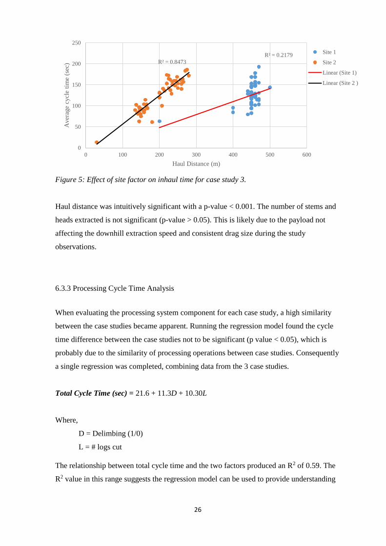
The relationship between skidder cycle time and the significant factors produced an R2
value of 0.38. This indicates the regression can be used as a useful guide for understanding
the factors affecting cycle time but not an accurate predictor.
The significant factors measured that affect cycle time were haul distance and site factor.
The likely reason for the difference in cycle time from site factor can be attributed to
differing ground conditions and piece size between site. Site 1 is stated to be have an
average cycle time 210 seconds quicker than site 2. Although this value appears
abnormally large, the factor provided a p value < 0.001. The apparent difference is shown
in figure 5, comparing inhaul time for each site against inhaul element time.
26
Figure 5: Effect of site factor on inhaul time for case study 3.
Haul distance was intuitively significant with a p-value < 0.001. The number of stems and
heads extracted is not significant (p-value > 0.05). This is likely due to the payload not
affecting the downhill extraction speed and consistent drag size during the study
observations.
6.3.3 Processing Cycle Time Analysis
When evaluating the processing system component for each case study, a high similarity
between the case studies became apparent. Running the regression model found the cycle
time difference between the case studies not to be significant (p value < 0.05), which is
probably due to the similarity of processing operations between case studies. Consequently
a single regression was completed, combining data from the 3 case studies.
Total Cycle Time (sec) = 21.6 + 11.3D + 10.30L
Where,
D = Delimbing (1/0)
L = # logs cut
The relationship between total cycle time and the two factors produced an R2 of 0.59. The
R2 value in this range suggests the regression model can be used to provide understanding
R² = 0.2179
R² = 0.8473
0
50
100
150
200
250
0 100 200 300 400 500 600
Aver
age
cycl
e ti
me
(sec
)
Haul Distance (m)
Site 1
Site 2
Linear (Site 1)
Linear (Site 2 )
27
of what affects the cycle time, however not used as predictor of cycle time, with 41% of
the variation not explained within the regression model.
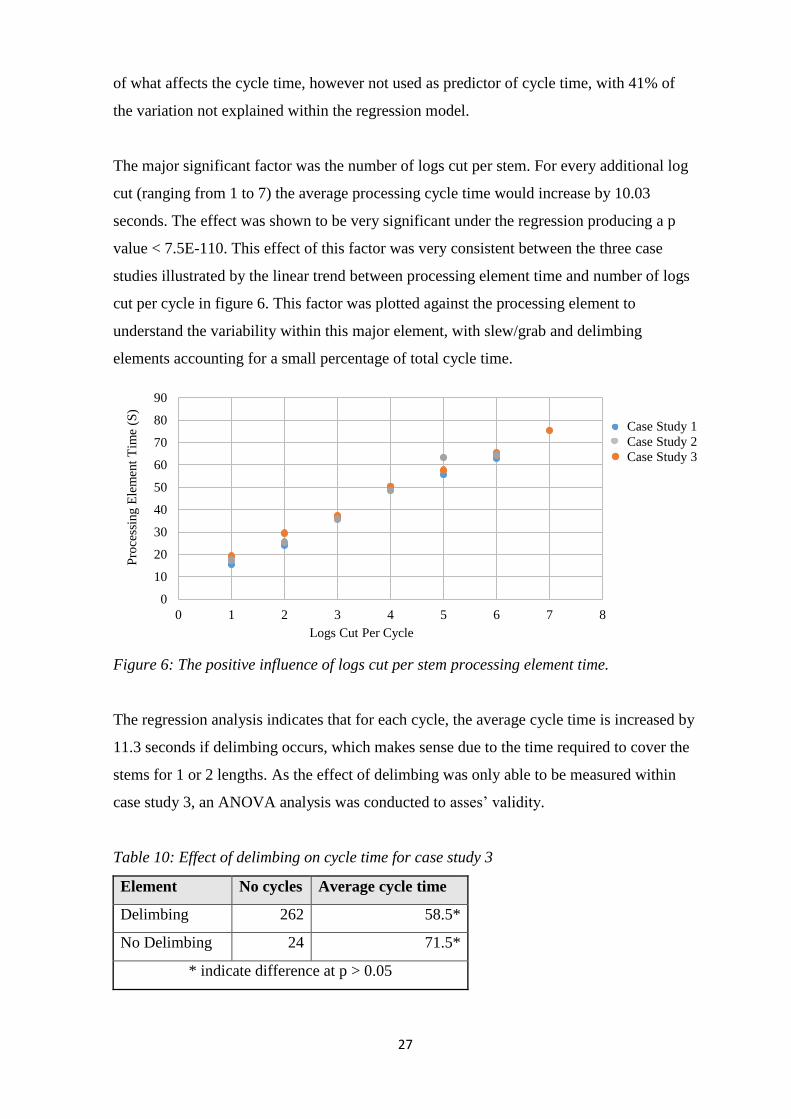
The major significant factor was the number of logs cut per stem. For every additional log
cut (ranging from 1 to 7) the average processing cycle time would increase by 10.03
seconds. The effect was shown to be very significant under the regression producing a p
value < 7.5E-110. This effect of this factor was very consistent between the three case
studies illustrated by the linear trend between processing element time and number of logs
cut per cycle in figure 6. This factor was plotted against the processing element to
understand the variability within this major element, with slew/grab and delimbing
elements accounting for a small percentage of total cycle time.
Figure 6: The positive influence of logs cut per stem processing element time.
The regression analysis indicates that for each cycle, the average cycle time is increased by
11.3 seconds if delimbing occurs, which makes sense due to the time required to cover the
stems for 1 or 2 lengths. As the effect of delimbing was only able to be measured within
case study 3, an ANOVA analysis was conducted to asses’ validity.
Table 10: Effect of delimbing on cycle time for case study 3
Element No cycles Average cycle time
Delimbing 262 58.5*
No Delimbing 24 71.5*
* indicate difference at p > 0.05
0
10
20
30
40
50
60
70
80
90
0 1 2 3 4 5 6 7 8
Pro
cess
ing E
lem
ent
Tim
e (S
)
Logs Cut Per Cycle
Case Study 1
Case Study 2
Case Study 3

28
Table 10 indicates a significant difference in cycle time if delimbing occurs or does not
occur. Average time difference between is 12 seconds indicating the validity of the
delimbing factor in understanding processing cycle time.
6.4 Productivity Analysis
A further regression study was conducted to estimate productivity of extraction operation
to evaluate the effects of observed factors on hourly extraction productivity. Productivity
regressions were run solely for extraction and not felling and processing components as a
single piece (average piece size) was processed or felled per cycle. Therefore it would be
assumed regressions would be equivalent to cycle time analyses. Productivity regression
equations for each of the case studies are as follows:
Case Study 1 (t/PMH) = 13.8 - 0.04HD + 13.5S + 3.06H - 6.9ST
Case Study 2 (t/PMH) = 53.7 - 0.24HD + 46.9S + 1.5H
Case Study 3 (t/PMH) = 56.7ST - 0.09HD + 22.01S + 5.1H
Where,
HD = haul distance (m)
S = number of stems extracted (per cycle)
H = number of heads extracted (per cycle)
ST = Site factor (1/0) (1 = site 1; 0 = site 2)
For all case studies the relationship between productivity and measured factors was much
stronger relationship than cycle time. Case study 1 saw the greatest shift in R2 value from
0.74 against 0.24 (cycle time relationship). Case study 3 also saw a great shift in R2 value
from the cycle time analysis, due to the same reasoning as case study 1. For case study 1
the R2 provided in the regression was 0.80 (cycle time analysis, R2 = 0.37, case study 1).
The greater R2 values imply that a larger proportion of the variation has been explained in
the regression, with equations for all case studies regressions providing a good
understanding and prediction of system productivity. These equations are therefore better

29
predictors than cycle time equations and more directly correlated to the effect of factors on
machine productivity rates.
The number of stems and heads extracted were not significant in the cycle time analysis,
however highly significant in the regression against hourly productivity. The number of
stems extracted was the most significant factor in the regression producing p values below
0.001 for all case studies. Understandably the number of stems and heads extracted per
drag became a significant when predicting productivity, due to the direct correlation with
cycle payload and hence hourly productivity. Heads were less significant for all case
studies presumably due to the smaller effect on payload.
An intriguing result was the effect of site factor on productivity for case study 3, which is
stated to decrease by a momentous 56.7t/PMH. Changes in productivity occurred for case
study 1 between sites, however the difference was only 6.9 t/PMH.
Haul Distance intuitively had a significant impact on hourly productivity. Haul distance
had the greatest impact on case study 2 where productivity decreased by 0.24t/PMH for
every additional metre (p value < 0.001).

30
7.0 Discussion
7.1 System Production Balance
The study of the three operations found large imbalances between felling, extraction and
processing which is typical of higher production mechanised operations (Evanson and
Amishev, 2012). The operational bottleneck for each case study was significantly lower
than the most productive operational phase. For each case study, felling was the most
productive phase with extraction the bottleneck for case studies 1 and 3, and processing for
case study 2. This differed to 2 fully mechanised swing yarder studies that found bunched
extraction and processing to be the most productive system components (Evanson and
Amsihev, 2009; Evanson and Amishev 2010). The production difference between
bottleneck and most productive component was however similar when comparing swing
yarder operations, with production differences of 37%, 28% and 37% for case study 2 and
the two alternate studies respectively (Evanson and Amsihev, 2009; Evanson and Amishev
2010). Extraction was the bottleneck in two of the three case studies which was similar to
the results of the two alternate studies. Unbunched extraction was the bottleneck at for
these studies, exhibiting productivity of 48.8m3/PMH (Evanson and Amsihev, 2009).
Increased productivity of the bottleneck and reduced felling productivity would be required
for each case study to balance system productivity and result in greater machine utilisation
rates. Processing would require a minor shift in productivity (excluding case study 2) due
to hourly production rates between bottleneck and felling system components.
7.2 Factors affecting Felling
Productivity of the felling machine was near double bottleneck productivity for case
studies 1 and 3. Productivity of the felling machine is understandably greater than other
system components due to the simplicity of the felling cycle. Shifting position between
stems significantly affected cycle time, however it would be impractical to shift machine
position between trees if deemed unnecessary, in order to provide a more balanced system.
The major factors that could be influenced to alter production would be increased bunching
and shovelling. Bunching was found to reduce productivity by 24.1m3/PMH and
20.9m3/PMH for each additional stem bunched for case studies 1 and 2. An alternate study

31
of a tethered felling machine found bunching (total stems bunched) to decrease
productivity by 29.6m3/PMH or 26% for the total cycle time (Evanson & Amishev, 2013).
The effect of bunching on productivity appears uncharacteristically high for case studies 1
and 3 (possibly due to the small sample size and single stem bunched per felling cycle)
however indicate the significance of the number of stems bunched on productivity.
Increased bunching would also aid extraction through reduced hook up time in mechanised
extraction operation. An earlier study evaluating the effects of bunched extraction versus
unbunched extraction saw an increase in productivity by 33% (Evanson & Amishev,
2009). With case studies 2 and 3 already employing shovelling/bunching excavators to aid
extraction, such machines could be utilised elsewhere with the felling machine performing
the duties of this machine.
Felling productivity for case studies 2 and 3 was near double the productivity of the
bottleneck (88% and 98% difference respectively). Influencing factors to balance
productivity is perhaps infeasible due to the large disparity between felling and bottleneck.
A potential solution to maintain high utilisation rates is to use felling machines across
multiple operations. This would however raise issues with transport costs and work
availability at alternate operations.
7.3 Factors affecting Extraction
The number of stems significantly affected productivity within operations, due to the direct
impact on payload. This factor appeared to have a stronger significance on productivity of
the cable yarding case studies compared to the ground based case study. Alternate
literature has also documented stems and payload significance on cable extraction
productivity compared with ground based extraction (Sunderburg & Silverside, 1996). In
harvesting systems the direct influence of the number of stems on productivity is well
recognised with workers attempting to maximise payload in order to capitalize on
productivity gains.
Inherently haul distance had the greatest impact on productivity for all case studies. Haul
distance is renowned as one of the major factors affecting the productivity of all harvesting
operations (Gardner, 1980). Haul distance was found to have the greatest affect in case
study 2 with a reduction in productivity of 0.25m3/PMH for every additional metre of haul

32
distance. Average haul distance would therefore need to be reduced in order to increase
extraction productivity. Increased roading density or two staging (where feasible) could
potentially reduce haul distance if the benefits of reduced haul distance outweigh the costs
of additional roading.
Haul distance however had lesser influence on extraction productivity for case study 1.
This is due to the relative short inhaul and outhaul phases in comparison to the hook-up
stage of the operation, accounting for half (47%) of average cycle time. Extensive hook-up
time was due to the time required for manual breaker-outs to attach stems and retreat to a
safe distance, before extracting the drag. To reduce hook up time, mechanisation could be
employed in a way of a mechanised grapple carriage. A study of the Falcon forestry claw
indicated the average hook-up time for the Falcon forestry claw on average (35.31
seconds) (Fairhall, 2014) was much quicker than hook-up with manual breaker outs
observed at case study 1. This however would only be appropriate at sites where there is
enough slope for gravity outhaul of the carriage (20%+)(Harill, 2014) due to the 2 drum
cable system in case study 1 with no available haul back line. The Mega Claw line grapple
carriage has the ability to operate on a running skyline system, although no studies have
been completed to test its effectiveness (Evanson & Parker, 2011).
Site factor was also a major factor affecting the extraction productivity for case study 3.
Average cycle time appeared relatively similar between sites however average haul
distance was much greater at site 1. The major variables differing between sites were piece
size, average slope (table 1) and ground conditions. Average piece size would affect
productivity to some extent, with a similar number of stems extracted per average cycle
between sites. Slope would have minimal effect as stems were shovelled from the steeper
terrain to skidder trails at both sites. The major factor can therefore be attributed with
differing ground conditions with observations occurring during summer and winter for
sites 1 and 2 respectively. During observations of site 2, the skidder was struggling to gain
traction on extraction trails, indicating the large inhaul and outhaul phases significantly
impacting cycle time and hence productivity. This provides implications for case study 3,
which would be more suited to work in stands with shorter haul distance during winter
months and larger stands during summer, to reduce the effect of site conditions on
productivity.

33
7.4 Factors affecting Processing
Processing cycle time was relatively similar between the three case studies, due to high
similarity of processing operations. Independent of average piece size, average cycle times
for each case study ranged between 0.93 and 1.34 minutes with case study 3 marginally
quicker due to the absence of delimbing. This cycle time was also consistent to another
study conducted by Evanson & Mcconchie (1996) with an average cycle time of 1.27
minutes.
The major factor affecting log processing was the number of logs cut per stem, with each
additional log cut reducing hourly productivity by 16%. This factor was very consistent
between all three studies with a linear increase in cycle time per log cut. The increase in
cycle time is simply due to the extra time required to pass over the stem and drop log in
appropriate pile. The number of logs cut is however dependent on meeting market
requirements and therefore cannot be changed to balance productivity. As two of the three
case studies lie between the bottleneck and the most productive system component,
altering productivity of the processing operation to balance productivity is of limited
importance.
Delimbing was also seen as a significant factor affecting average cycle time due to the
additional time required to pass the processing head over the stem. The effect of delimbing
had a much smaller effect on cycle time than reported by Evanson & Mcconchie (1996),
who found delimbing to increase cycle time by 34 seconds in comparison to 11.3 seconds
observed at case study 3. Removal of delimbing at the landing is only achievable for case
study 3 as delimbing occurs within the field by the felling machine. Delimbing during
felling cycles within semi-mechanised cable yarding case systems would also be less
applicable due to reduced safety of breaker-outs from slippery and moving stems.
7.5 Further Analysis
The three case studies have shown that mechanised systems are often not well balanced
and result in system components being underutilised. An approach to increase utilisation
rates from more balanced systems is through task strategies and machine sharing between
systems. Altering task strategies and system setup to gain more balanced systems, could

34
prove uneconomic. Additional studies should occur analysing the true effects on costs from
altering harvesting and task strategies in order to gain balanced systems. This will provide
justification of management and planning decisions to achieve more balanced systems and
the true costs of such activities.
An implication for NFL is that limited studies have been carried out on the capability of
systems following the introduction of felling machines. The information provided from this
study can be used as a base case for further study, categorising system performance on a
variety of terrain classes. Further studies can be completed on a variety of terrain classes
for these case studies and compared against base case data to understand machine and
system capability. Greater system understanding can be used by management to situate
operations in appropriate locations, based on machine and operational capability.
7.5 Limitations
A limitation of data collection is that the detailed time and motion study only takes a
snapshot of a limited number of operations. Forestry operations are very complex with a
wide range factors (e.g. slope or piece size) affecting machine productivity rates. The
sample collected during data collection therefore does not provide an accurate
representation of each system, and other harvesting systems of similar makeup. During
observations, machine operators were also aware that they were subjects of a study, which
may have altered work behaviour (known as the Hawthorne effect) and resulted in non-
representative data collected. This study should therefore only be used to assist with the
understating of harvesting production balance on steeper terrain and associated factors
affecting productivity.
Throughout analyses, delay elements were not accounted for due to the small sample of
observed delays. Specific operations observed that would likely influence cycle time and
hence productivity include line shifts for tethered felling machines and tail hold shifts of
the cable yarders. Although these delays are not part of the common working cycle, they
are required to be productive and therefore should be included in the analysis to gain
accurate system component production rates.
During studies of the extraction operation, multiple locations were observed to achieve a
sufficient number of cycles for an analysis. This issue associated with multiple study sites

35
is the variation of site factors that can significantly affect machine productivity. Varying
factors observed between study sites were terrain, piece size, weather and operation setup.
Extraction productivity rates provided will likely be under/overestimated, affecting the
production balance results presented for each case study.
Cycle elements for felling operations were often short and performed in an unpredictable
sequence. Delineation of cycle elements was difficult to achieve, resulting in the
probability of slightly incorrect cycle element measurements. Felling machines were
occasionally out of view while observing their activity, which could have also produced
incorrect cycle element measurements.
Haul distance throughout the study was calculated with scale maps and range finders for
case study 3. As it was unsafe to measure haul distance on foot, assumptions of distance
were made to best possible judgement, based on the range finder and scale map
measurements. Haul distances for case study 3 are consequently likely to be less accurate
than distances for case studies 1 and 2.

36
8.0 Conclusion
The initial objective of this study was to understand the system production balance that
occurred within three mechanised harvesting case studies. Across the three case studies it
large production imbalances were apparent between felling, extraction and processing.
Felling was by far the most productive phase, near doubling bottleneck production rates of
case studies 1 and 3. Production of the felling operation was 98%, 37% and 88% more
productive than the bottleneck for case studies 1, 2 and 3 respectively. System bottlenecks
for case studies 1 and 3 was extraction, whereas case study 2 was processing. (Although
very similar to extraction; 79.1m3/PMH vs 72.4m3/PMH). To balance system productivity
across all case studies, felling operations are required to significantly reduce productivity
with the system bottleneck significantly increase productivity.
The major aim of the study was to understand factors affecting system component
productivity rates to aid planning in order to achieve more balanced systems. Measured
factors affecting felling were the number of stems shovelled, the number of stems bunched,
wind throw interference and machine position shift (case study 3). For every stem
bunched, average productivity decreased by 35% (24m3/PMH) and 21% (20.9m3/PMH) for
case studies 2 and 3 respectively. Every additional stem shovelled increased average cycle
time by 7.5 seconds, resulting in a productivity shit of 7.4m3/PMH for case study 2.
Factors affecting cycle time of extraction operations were haul distance, the number of
stems extracted and site factor. Haul distance and the number of stems extracted had the
greatest impact on hourly productivity for case study 2 (of the three case studies), due to
shorter cycle time and greater hourly productivity. Site factor affected hourly productivity
by 6.9m3/PMH and 56.7m3/PMH for case studies 1 and 3 respectively. The difference in
productivity can be largely attributed to yarding systems (shotgun vs scab) for case study 1
and site conditions for case study 3.
Processing was affected by the number of logs cut per stem and if delimbing occurred. For
every additional log processed per cycle, productivity decreased by 14%. Delimbing
decreased productivity by an average of 16% with processing head requiring time to pass
over the stem, increasing cycle time.

37
9.0 References
Acuna, M., Bigot, M., Guerra, S., Hartsough, B., Kanzian, C., Kärhä, Talbot, B.
(2012). Good practice guidelines for biomass production studies.
Adams, G., Amrstrong, H., & Cosman , M. (2014). Independent Forestry Safety Review -
An agenda for change in the forestry sector.
Amishev, D. (2012). Mechanised Steep Slope Felling for New Zealand - Current
Developments. FFR Harvesting Technical Note, HTN04-07.
Amishev, D. (2011). Steep Slope Feller Buncher: A Feasibility Study. FFR Report FFR-
H007, 30.
Bentley, T. A., Parker, R. J., & Ashby, L. (2005). Understanding felling safety in the New
Zealand forest industry. Applied Ergonomics, 36(2), 165-175.
Evanson, T., & Amishev, D. (2009). A new method for bunching trees on steep
terrain. FFR Technical Note, 2(5), 1-9.
Evanson, T., & Amishev, D. A. (2012). Steep Slope Excavator Feller Buncher. FFR
Harvesting Technical Note, 3(2).
Evanson, T., & Amishev, D. (2013). ClimbMAX2 Steep Slope Harvester . FFR Harvesting
Techical Note, HTN05-07.
Evanson, T., & McConchie, M. (1996). Productivity measurements of two Waratah 234
hydraulic tree harvesters in radiata pine in New Zealand.Journal of Forest
Engineering, 7(3), 41-52.
Fairhall, J. (2014). Terrain Dependent Harvesting Productivity and Mechanised Yarding
Evaluation. Christchurch.
Harrill, H. (2014). Improving Cable Logging Operations for New Zealand’s Steep Terrain
Forest Plantations.
Holzleitner, F., Stampfer, K., & Visser, R. (2011). Utilization rates and cost factors in
timber harvesting based on long-term machine data. Croatian Journal of Forest
Engineering, 32(2), 501-508.
Mușat, E. C., Apăfăian, A. I., Ignea, G., Ciobanu, V. D., Iordache, E., Derczeni, R. A., ...
& Borz, S. A. (2015). Time expenditure in computer aided time studies
implemented for highly mechanized forest equipment. Annals of Forest Research,
1-16.
Olsen, E. D., Hossain, M. M., & Miller, M. E. (1998). Statistical comparison of methods
used in harvesting work studies. Corvallis, Or.: College of Forestry, Forest
Research Laboratory, Oregon State University.
Pan, F., Han, H. S., Johnson, L. R., & Elliot, W. J. (2008). Production and cost of
harvesting, processing, and transporting small-diameter (<= 5 inches) trees for
energy. Forest Products Journal, 58(5), 47.

38
Perneger, T. V. (1998). What's wrong with Bonferroni adjustments. Bmj, 316(7139), 1236-
1238.
Pfeiffer, K. (1967). Analysis of methods of studying operational efficiency in
forestry (Doctoral dissertation, University of British Columbia).
Raymond, K. (2010). Steep country harvesting-" innovative harvesting solutions' A step
change harvesting research programme. New Zealand Journal of Forestry, 55(9).
Raymond, K. (2012). Innovation To Increase Profitability Of Steep Terrain Harvesting In
New Zealand. New Zealand Journal of Forestry, 57, 19-23.
Riddle, A. (1995). Mechanisation of logging operations in New Zealand. New Zealand
Forestry, 11, 17-22.
Saathof, D. (2014). An investigation of the measurement accuracy and productivity of a
Waratah HTH 625c Processor Head.
Smidt, M., Tufts, R., & Gallagher, T. (2009). Logging efficiency and cost.ANR-1347-
Alabama Cooperative Extension System.
Stihl Shop - Stihl Shop. (2016). Retrieved from Stihl Shop:
https://www.stihlshop.co.nz/search.aspx?q=660
Visser, R., Raymond, K., & Harrill, H. (2014a). Developing Fully Mechanised Steep
Terrain Harvesting Operations.
Visser, R., Raymond, K., & Harill, H. (2014b). Mechanising steep terrain harvesting
operations. NZ Journal of Forestry, 59(3).

39
10.0 Appendix
10.1 Study Location Slope Maps
Case Study 1
Appendix Figure 2: Slope map of second study site
for case study 1 at Long Gully, Golden Downs forest.
Appendix Figure 1: Slope map of study site for case
study 1 at Western Boundary, Golden Downs forest.

40
Case Study 2
Appendix Figure 3 and 4: Slope maps for case study 2 study site, Brightwater block
Appendix Figure 5: Slope maps for case study 2 second study site, Oliver’s
block, Golden Downs forest.

41
Case Study 3
Appendix Figure 7: Slope map of the second study
site for case study 3, Fairacres block, Wairau South
Appendix Figure 6: Slope map of the first study site of
case study 3, Pascoes block, Golden Downs

42
10.2 Regression Outputs
Felling Cycle Time
Appendix table 1: Regression output for felling cycle time of case study 1.
Regression Output
Multiple R 0.83
R Square 0.69
Adjusted R Square 0.68
Standard Error 40
Observations 204
Coefficients Standard Error t Stat P-value
Intercept 33 6.4 5.2 4.9E-07
Bunching (1/0) -3.1 8.2 -0.4 0.70
Stems Bunched 34 2.1 16 7.8E-38
Position Shift (1/0) 27 6.8 4.0 8.8E-05
Appendix table 2: Regression output for felling cycle time of case study 2.
Regression Output
Multiple R 0.50
R Square 0.25
Adjusted R Square 0.24
Standard Error 38
Observations 220
Coefficients Standard Error t Stat P-value
Intercept 31 5.6 5.6 5.10E-08
Stems shovelled 11 3.9 2.7 0.0075
Stems Bunched 21 5.7 3.8 0.00022
Position Shift (1/0) 39 5.3 7.4 3.2E-12
Shovelling (1/0) -11 10 -1.1 0.29
Appendix table 3: Regression output for felling cycle time of case study 3.
Regression
Output
Multiple R 0.61
R Square 0.37
Adjusted R Square 0.36
Standard Error 37
Observations 173
Coefficients Standard Error t Stat P-value
Intercept 56 7.3 7.6 1.9E-12
Wind throw (1/0) 68 6.8 10.0 7.2E-19
Position Shift (1/0) 6.1 7.8 0.78 0.44
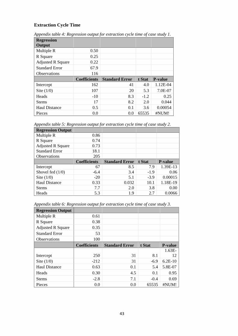
43
Extraction Cycle Time
Appendix table 4: Regression output for extraction cycle time of case study 1.
Regression
Output
Multiple R 0.50
R Square 0.25
Adjusted R Square 0.22
Standard Error 67.9
Observations 116
Coefficients Standard Error t Stat P-value
Intercept 162 41 4.0 1.12E-04
Site (1/0) 107 20 5.3 7.0E-07
Heads -10 8.3 -1.2 0.25
Stems 17 8.2 2.0 0.044
Haul Distance 0.5 0.1 3.6 0.00054
Pieces 0.0 0.0 65535 #NUM!
Appendix table 5: Regression output for extraction cycle time of case study 2.
Regression Output
Multiple R 0.86
R Square 0.74
Adjusted R Square 0.73
Standard Error 18.1
Observations 205
Coefficients Standard Error t Stat P-value
Intercept 67 8.5 7.9 1.39E-13
Shovel fed (1/0) -6.4 3.4 -1.9 0.06
Site (1/0) -20 5.1 -3.9 0.00015
Haul Distance 0.33 0.032 10.1 1.18E-19
Stems 7.7 2.0 3.8 0.00
Heads 5.3 1.9 2.7 0.0066
Appendix table 6: Regression output for extraction cycle time of case study 3.
Regression Output
Multiple R 0.61
R Square 0.38
Adjusted R Square 0.35
Standard Error 53
Observations 100
Coefficients Standard Error t Stat P-value
Intercept 250 31 8.1
1.63E-
12
Site (1/0) -212 31 -6.9 6.2E-10
Haul Distance 0.63 0.1 5.4 5.8E-07
Heads 0.30 4.5 0.1 0.95
Stems -2.8 7.1 -0.4 0.69
Pieces 0.0 0.0 65535 #NUM!

44
Extraction Productivity
Appendix table 7: Regression output for hourly extraction productivity of case study 1.
Regression
Output
Multiple R 0.86
R Square 0.74
Adjusted R Square 0.73
Standard Error 7.3
Observations 116
Coefficients Standard Error t Stat P-value
Intercept 14 4.4 3.2 1.95E-03
Haul Distance -0.037 0.016 -2.3 0.0210
Stems 14 0.88 15.4 2.3E-29
Heads 3.1 0.90 3.4 0.00087
Site (1/0) -7.0 2.2 -3.2 0.0017
Pieces 0.0 0.0 65535 #NUM!
Appendix table 8: Regression output for hourly extraction productivity of case study 2.
Regression Output
Multiple R 0.94
R Square 0.88
Adjusted R Square 0.88
Standard Error 12.9
Observations 205
Coefficients Standard Error t Stat P-value
Intercept 56 6.1 9.2 6.37E-17
Shovel fed (1/0) 3.6 2.4 1.5 0.15
Site (1/0) -21 3.7 -5.8 0.00000
Haul Distance -0.24 0.023 -10.5 6.6E-21
Stems 45 1.4 32.0 0.00
Heads 4.7 1.4 3.4 0.00081
Appendix table 9: Regression output for hourly extraction productivity of case study 3.
Regression Output
Multiple R 0.89
R Square 0.81
Adjusted R Square 0.79
Standard Error 12.9
Observations 100
Coefficients Standard Error t Stat P-value
Intercept -4 7.6 -0.48 6.35E-01
Site (1/0) 56 7.6 7.5 3.54E-11
Haul Distance -0.094 0.029 -3.3 0.00154
Stems 22 1.75 12.6 5.46E-22
Heads 5.1 1.1 4.6 1.50E-05
Pieces 0.0 0.0 65535 #NUM!

45
Processing Cycle Time
Appendix table 10: Regression output for processing cycle time of all three case studies.
Regression Output
Multiple R 0.70
R Square 0.49
Adjusted R Square 0.49
Standard Error 18
Observations 871
Coefficients Standard Error t Stat P-value
Intercept 25 4.1 6.0 2.3E-09
Logs Cut 11 0.4 25.9 7.5E-110
Case study 3 -4 3.8 -1.0 0.33
Case Study 2 3 1.6 1.8 0.074306
Delimbing (1/0) 11 4 3.0 0.0032


