International Journal of Assessment Tools in Education
2018, Vol. 5, No. 2, 248–262
DOI: 10.21449/ijate.407193
Published at http://www.ijate.net http://dergipark.gov.tr/ijate Research Article
248
An Iterative Method for Empirically-Based Q-Matrix Validation
Ragip Terzi 1*, Jimmy de la Torre 2
1 Educational Measurement and Evaluation, Harran University, Sanliurfa, Turkey 2 Division of Learning, Development and Diversity, The University of Hong Kong, Pokfulam, Hong Kong
Abstract: In cognitive diagnosis modeling, the attributes required for each item are specified in the Q-matrix. The traditional way of constructing a Q-matrix based on expert opinion is inherently subjective, consequently resulting in serious validity concerns. The current study proposes a new validation method under the deterministic inputs, noisy “and” gate (DINA) model to empirically validate attribute specifications in the Q-matrix. In particular, an iterative procedure with a modified version of the sequential search algorithm is introduced. Simulation studies are conducted to compare the proposed method with existing parametric and nonparametric methods. Results show that the new method outperforms the other methods across the board. Finally, the method is applied to real data using fraction-subtraction data.
ARTICLE HISTORY
Received: 02 February 2018 Revised: 14 March 2018 Accepted: 15 March 2018
KEYWORDS
Cognitive diagnosis model, Q-matrix validation, DINA, sequential search algorithm
1. INTRODUCTION Cognitive diagnosis models (CDMs) require a Q-matrix (Tatsuoka, 1983) to identify the
specific subset of attributes measured by each item. The entry qjk in row j and column k of the Q-matrix is 1 if the 𝑘𝑡ℎ attribute is required to correctly answer item j, and 0 otherwise. Due to its nature, constructing a Q-matrix is usually subjective, which has raised serious validity concerns among researchers. For instance, the estimation of model parameters, and ultimately the accuracy of attribute classifications may be negatively affected by including or omitting multiple q-entries in the Q-matrix (de la Torre, 2011; Rupp & Templin, 2008). However, the Q-matrix is usually assumed to be correct once specified by domain experts. This assumption is generally made because until recently, few well-established methods have become available to detect misspecifications in the Q-matrix (Chiu, 2013; de la Torre, 2008; Rupp & Templin, 2008), particularly when general CDMs are involved (de la Torre & Chiu, 2016; Liu, Xu, & Ying, 2012; Terzi, 2017). Any analysis, such as model-fit evaluation, that does not check the correctness of the Q-matrix, becomes questionable.
CONTACT: Ragıp Terzi [email protected] Harran University, School of Education, E Blok, Osmanbey Yerleskesi, 63190, Sanliurfa, Turkey
This study is derived from a part of Ph.D. dissertation of the first author.
ISSN-e: 2148-7456 /© IJATE 2018
Terzi & de la Torre
249
These concerns have led to developments of some statistical methods for validating the appropriateness of Q-matrix specifications. One of the earlier studies on the Q-matrix validation was introduced by de la Torre (2008) for the deterministic inputs, noisy “and” gate (DINA; Haertel, 1989; Junker & Sijtsma, 2001) model. It is an empirically based δ-method that defines the correct q-vector for each item. In doing so, the discrimination index of item j, 𝛿𝑗, is estimated. The index 𝛿𝑗 is the difference in the probabilities of correct responses between examinees who have mastered the required attributes and those who have not. Using the δ-method, two algorithms were discussed in de la Torre (2008). However, the algorithms have some limitations. As noted by de la Torre (2008), an incorrect Q-matrix because of over- and under-specifications of attributes can cause bias in parameter estimation. This issue cannot be completely addressed by the algorithms because they usually choose q-vectors with all attributes specified. For one of the algorithms, the sequential search algorithm (SSA), it is also not clear what cut-off values should be used in practice because it could vary depending on many conditions, such as changes in sample sizes, test lengths, item qualities, and amount of misspecifications, all of which were fixed in de la Torre (2008)'s paper. It should also be noted that the algorithm was not implemented iteratively, meaning that the validation method stops after one full iteration even if changes are made in the provisional Q-matrix.
Another method, the Q-matrix refinement method (QRM), was proposed by (Chiu, 2013) based on a nonparametric classification procedure (Chiu & Douglas, 2013). This method aims to minimize the residual sum of squares (RSS) between the observed and ideal responses among all the possible q-vectors given a Q-matrix. The RSS is used to identify any misspecified q-entries for an item. In the algorithm, the item vector with the highest RSS gets replaced by the one having the lowest RSS. The process is repeated iteratively until the convergence criterion is met. Due to its nature as a nonparametric method, it neither relies on the estimation of model parameters nor makes any assumptions other than those made by the CDM itself (Chiu, 2013). However, if the underlying model is known, parametric methods should provide more powerful results particularly when N is large.
DeCarlo (2011) introduced a model-based approach using a Bayesian extension of the DINA model. In this method, possible misspecified entries in the Q-matrix were identified in advance. Then, these entries were treated as random (Bernoulli) variables and estimated with the rest of the model parameters. Limitations of this method are that it is computationally time-consuming and any misspecified q-entries have to be identified in advance. Unlike DeCarlo (2011)'s study, Liu et al. (2012) proposed a data-driven approach in that any expert involvement in Q-matrix design is not required for identifying misspecified entries in the Q-matrix. However, when unknown guessing parameters exist, the identifiability of the Q-matrix can be difficult.
Recently, de la Torre and Chiu (2016) developed a discrimination index, as an extension of the empirically based δ-method (de la Torre, 2008), using the G-DINA model. This index can be applied under a wider class of CDMs. However, the findings of the study were limited to the fixed sample size and test length. Moreover, the index does not determine optimal ε values that prevent q-entries from over- or under-specifications, and the procedure is not iterative, meaning that it stops further identifying attribute specifications after the first round of validation step.
The purpose of this current study is to introduce an iterative procedure in conjunction with a modified version of the SSA, and is called iterative modified SSA (IMSSA). The new method aims to make three crucial contributions to the Q-matrix validation literature. First, using simulation, an approximation was made to generally define an empirically based a cut-off value applicable across all conditions. Second, the search algorithm only focuses on single-attribute specifications so that it can eliminate additional complications that could happen due
Int. J. Asst. Tools in Educ., Vol. 5, No. 2, (2018) pp. 248-262
250
to q-vectors with more than single-attribute specifications. Third, the algorithm is implemented iteratively, such that, if any q-vectors are changed in the previous iteration, a new calibration is carried out using the updated Q-matrix as the provisional Q-matrix. The iterative algorithm aims to alleviate negative effects of any misspecified attribute specifications given in the preceding iteration. In this present study, iterative and non-iterative algorithms were compared to examine if an iterative algorithm can further identify and correct misspecifications in succeeding iterations.
Given the purpose, the rest of the paper consists of the following sections: First is a brief background on the DINA model, Q-matrix refinement method, and exhaustive and sequential search algorithms. Second is a presentation of the new method proposed in this paper. This is followed by simulation study design and results. Then, real data analysis and its results are introduced. Finally, the paper concludes with a discussion and conclusion for future studies.
2. BACKGROUND 2.1. The DINA Model
The DINA model has been commonly used in many studies (e.g., de la Torre & Douglas, 2004, 2008; de la Torre, 2009a; DeCarlo, 2011; Kuo, Pai, & de la Torre, 2016; Liu, Ying, & Zhang, 2015; Park & Lee, 2014; Rupp & Templin, 2008). This study focuses on the DINA model because of its more straightforward interpretations, smaller sample size requirements for accurate parameter estimation (Rojas, de la Torre, & Olea, 2012), and flexibility for extension to more general cognitive diagnostic models. The DINA model is an example of a conjunctive model for dichotomously scored test items, where all required attributes of an item should be mastered by examinees before an examinee can be expected to correctly answer the item. Nonmastery of one or more required attributes for an item is equivalent to nonmastery of all required attributes. Let examinee i’s binary attribute vector be denoted by 𝜶𝑖 = {𝛼𝑖𝑘}. The item response function of the model is defined as:
𝑃 (𝑋𝑖𝑗 = 1|𝛼𝑖) = (1 − 𝑠𝑗)
𝜂𝑖𝑗𝑔𝑗
(1−𝜂𝑖𝑗), (1)
which is the probability of answering an item j correctly by examinees with the attribute pattern 𝜶𝑖, 𝑋𝑖𝑗 is the response of examinee i (i = 1, 2, …, N) to item j (j = 1, 2, …, J), and 𝜂𝑖𝑗 is the ideal response computed as:
𝜂𝑖𝑗 = ∏ 𝛼𝑖𝑘𝑞𝑗𝑘𝐾
𝑘=1 , (2)
an indicator of whether all of the required attributes associated with item j have been mastered by examinee i.
2.2. Q-Matrix Refinement Method The RSS of item j across all examinees is defined as:
K
mm Cijmij
N
iijijj XXRRS
2
1
2
1
2 , (3)
where ijX and ij are the observed and ideal item responses of examinee i to item j, respectively, 𝐶𝑚 is the latent proficiency class m, and N is the number of examinees. Note that the index j of 𝜂𝑖𝑗 in Equation 3 was replaced by m because ideal item responses are class-

Terzi & de la Torre
251
specific, meaning that every examinee in the same latent class is assumed to have the same ideal response to an item (Chiu, 2013).
2.3. Exhaustive Search Algorithm The exhaustive search algorithm (ESA) for Q-matrix validation computes 𝛿𝑗𝑙 for all 𝑙 =
2𝐾 – 1 possible q-vectors for each j item (de la Torre, 2008). The q-vector that gives the largest difference in the probabilities of correct response between examinees who have all the required attributes (𝜂𝑗𝑙 = 1) and those who do not have (𝜂𝑗𝑙 = 0) among all the possible attribute patterns is chosen as the correct q-vector for item j. However, the algorithm becomes impractical when K is reasonably large. Additionally, the ESA has the tendency to choose over-specified q-vectors (de la Torre, 2008).
2.4. Sequential Search Algorithm The sequential search algorithm (SSA), in comparison to the ESA, is considered more
efficient because it does not require the comparisons of 𝛿𝑗𝑙 for all the possible attribute patterns. More specifically, 𝛿𝑗𝑙 is computed for (𝐾𝑗 + 1)𝐾 − (𝐾𝑗
2 + 𝐾𝑗)/2 q-vectors for item j, where 𝐾𝑗 is the number of attributes required for item j (de la Torre, 2008).
The SSA starts by comparing 𝛿𝑗𝑙1 of single-attribute q-vectors with the superscript (1)
referring to single-attribute q-vectors. Let 𝛿𝑗1 be the largest of 𝛿𝑗𝑙
1 from single-attribute q-vectors, and assume that this is due to 𝛼1. The process continues by examining 𝛿𝑗𝑙 of two-attribute q-vectors, 𝛿𝑗
2, where 𝛼1 is one of the required attributes. If 𝛿𝑗𝑙2 > 𝛿𝑗𝑙
1 , the single-attribute q-vector is replaced by a two-attribute q-vector. However, if 𝛿𝑗𝑙
1 > 𝛿𝑗𝑙2, the process is
terminated choosing 𝛼1 as the correct attribute specification for the q-vector. Otherwise, the process continues with such comparisons until a K-attribute q-vector is chosen as long as the difference of succeeding 𝛿𝑗𝑙 values (i.e., �̂�
𝑗
(𝐾𝑗+1)− �̂�
𝑗
(𝐾𝑗)) is larger than a predetermined cut-off value.
As stated earlier, estimation that involves some misspecified q-vectors can affect the quality of parameter estimation (Rupp & Templin, 2008) and this in turn affects the accuracy of the validation method. Similarly, the noise due to the stochastic nature of the response process makes it possible to obtain a q-vector with more attribute specifications than necessary. Especially using real data can cause �̂�
𝑗
(𝐾𝑗+1)> �̂�
𝑗
(𝐾𝑗) or the reverse, resulting in over- or under-specifications, respectively. A suggested solution is to assign ε, which is a minimum increment in the discrimination index of the item before an additional attribute can be included, as in, �̂�
𝑗
(𝐾𝑗+1)− �̂�
𝑗
(𝐾𝑗)> 휀 (de la Torre, 2008).
3. THE PROPOSED METHOD 3.1. An Iterative Method for Empirically-Based Q-Matrix Validation
This study introduces an iterative procedure in conjunction with a modified version of the SSA, and is called iterative modified SSA (IMSSA). The IMSSA differs from the SSA in two respects. First, the IMSSA determines required attribute specifications based on only the single-attribute q-vectors. Similar to the empirically based δ-method (de la Torre, 2008), the IMSSA starts by estimating the item parameters via an empirical Bayesian implementation of the expected-maximization (EM) algorithm (de la Torre, 2009b) using a provisional Q-matrix. The K numbers of �̂�s corresponding to the single-attribute q-vectors (i.e., 𝛿𝑗
1) are then estimated and ordered from the highest to the lowest. The correct attribute specification is determined

Int. J. Asst. Tools in Educ., Vol. 5, No. 2, (2018) pp. 248-262
252
based on the proportion of �̂�𝑗𝑙∗1 relative to the maximum �̂�𝑗(max)
1 (i.e., �̂�𝑗𝑙∗1 /�̂�𝑗(max)
1 , for 𝑙∗ =
1,2, … , 𝐾) for item j. �̂�𝑗(max)1 is �̂�𝑗𝑙∗=1
1 because it corresponds to the best suggested attribute specification. The noise due to the use of the estimated posterior distribution should be controlled so as to not cause any over- or under-specifications. That can be done by using a cut-off point denoted by 휀(1), which represent the minimum ratio between single-attribute q-vectors and the best single-attribute q-vector corresponding to �̂�𝑗(max)
1 . Specifically, if �̂�𝑗21 is
considerably smaller than �̂�𝑗(max)1 (i.e., �̂�𝑗2
1 /�̂�𝑗(max)1 < 휀(1) , the required attribute would be an
attribute specified in the single-attribute q-vector corresponding to �̂�𝑗(max)1 ; if not, the attribute
specifications in the first two q-vectors are chosen. It continues by checking the ratio �̂�𝑗3
1 /�̂�𝑗(max)1 . If the ratio is larger than 휀(1), the attribute specification in the third q-vector is also
added on the top of the previous two specifications, and it continues; otherwise, the process is terminated. The ratio between �̂�𝑗𝑙∗
1 and �̂�𝑗(max)1 was determined based on some preliminary
findings, and the values of 휀(1), the cut-off point, were defined using simulated response data. At this point, an example can be helpful to lay out the rationale as to how the study
determines the correctness of attribute specifications based on the ratio of �̂�s to the maximum �̂�. For illustration purposes, we considered two items, each with a misspecified attribute specification. In practice, the provisional Q-matrix may not have entirely correct specifications. However, data based on parameter estimates using the provisional Q-matrix can be generated. The �̂�-computation for the simulated data can be monitored, which can allow us to define extreme changes in the ratio of �̂�s.
Examples of �̂�𝑗𝑙∗1 computations for the simulated data can help determine whether or not
the algorithm could identify correct specifications. Assume that K = 5. Table 1 displays examples of items that have over- and under-specifications. In the first misspecification, the q-vector (1,0,0,0,0)′ is over-specified as in (1,0,1,0,0)′. The EM estimation is carried out with the latter q-vector, and �̂�s of single-attribute q-vectors are estimated and sorted from the highest to the lowest. The result suggests that the correct attribute specification is only 𝛼1 (�̂�𝑗(max)
1 =
.41) due to a large drop in �̂�𝑗21 (i.e., �̂�𝑗2
1 /�̂�𝑗(max)1 = .15 < 휀(1)), in that a value of 휀(1) will be
determined later. A similar result is also observed for an item that has been under-specified. The misspecification appears as (1,0,0,0,0)′ from the correct vector of (1,1,0,0,0)′ in the right-hand side of Table 1. The ratio of the second �̂�𝑗2
1 to the maximum �̂�𝑗(max)1 shows a small drop
(i.e., �̂�𝑗21 /�̂�𝑗(max)
1 = .73 > 휀(1)); however, the next ratio is rather small (i.e., �̂�𝑗31 /�̂�𝑗(max)
1 =
.13 < 휀(1)). Therefore, the attributes in the first two single-attribute q-vectors are accurately specified (i.e., 𝛼1 and 𝛼2). Note that the criterion is similar to the method proposed by de la Torre and Chiu (2016), which is the proportion of variance accounted for (PVAF) by a particular q-vector relative to the maximum �̂�2 that is achieved when all the attributes are specified (i.e., (1,1,1,1,1)′). However, the criterion in this study is not exactly the same, because it is relative to the best attribute specification, not the attribute vector with all the attributes specified.
Second, the IMSSA becomes more efficient than the original SSA because �̂� is not computed beyond single-attribute vectors. As such, the maximum number of comparisons for the new algorithm is K, which is considerably smaller than SSA (i.e., (𝐾𝑗 + 1)𝐾 − (𝐾𝑗
2 +
𝐾𝑗)/2) and ESA (i.e., 2𝐾 − 1), where K is the total number of attributes and 𝐾𝑗 is the number of attributes being measured by item j. For example, let 𝐾 = 10 and 𝐾𝑗 = 3. The maximum number of comparisons is 10 for the IMSSA, 34 for the SSA, and 1023 for the ESA. Thus, using the IMSSA can lessen complications associated with multiple search steps. In summary,

Terzi & de la Torre
253
examining the proportion of �̂� by a particular single-attribute q-vector to the maximum �̂� using a provisional q-vector could suggest which attributes should be specified -- �̂� of required attributes are considerably larger compared to �̂� of other attributes.
Table 1. Examples for Over- and Under-Specifications (1,0,0,0,0)′ → (1,0,1,0,0)′ (1,1,0,0,0)′ → (1,0,0,0,0)′
𝑙∗ 𝛼1 𝛼2 𝛼3 𝛼4 𝛼5 �̂�𝑗𝑙∗1
�̂�𝑗𝑙∗1
/�̂�𝑗(𝑚𝑎𝑥)1
𝛼1 𝛼2 𝛼3 𝛼4 𝛼5 �̂�𝑗𝑙∗1
�̂�𝑗𝑙∗1
/�̂�𝑗(𝑚𝑎𝑥)1
1 1 0 0 0 0 .41 1.00 √ 1 0 0 0 0 .40 1.00 √
2 0 0 1 0 0 .06 0.15 0 1 0 0 0 .29 0.73 √
3 0 0 0 0 1 .04 0.10 0 0 0 0 1 .05 0.13
4 0 1 0 0 0 .04 0.10 0 0 1 0 0 -.01 -0.03
5 0 0 0 1 0 -.00
0.00 0 0 0 1 0 -.03
-0.08
Note. The symbol √ displays the chosen attributes based on the associated δ-ratio. (1,0,0,0,0)′ → (1,0,1,0,0)′: (1,0,0,0,0)′ is over-specified as in (1,0,1,0,0)′. (1,1,0,0,0)′ → (1,0,0,0,0)′: (1,1,0,0,0)′ is under specified as in (1,0,0,0,0)′. Negative values in the ratio come from the negative δ̂. For example, .52 and .49 for the slip and guessing parameters, respectively, δ̂jl∗=4
1 =
1 − sjl∗=4 − gjl∗=4 = 1 − .52 − .49 = −.03.
4. SIMULATION STUDY DESIGN To evaluate the viability of the proposed method, two simulation studies were conducted
with the following goals: (1) to determine an optimal 휀(1) value, which could be generalized across the conditions; and (2) to compare the effectiveness of different validation methods with an iterative and noniterative algorithm. For each simulation condition, 100 datasets were replicated using the DINA model with the following factors: sample sizes (N = 1,000 and 2,000), test lengths (J = 15 and 30), item qualities (𝑠𝑗 = 𝑔𝑗 = 0.1, 0.2, and 0.3), and amount of misspecifications (5% and 10%). In this study, the three sets of item qualities were considered similar to Hou, de la Torre, and Nandakumar (2014). In each condition, 100 misspecified Q-matrices were generated, which contain 5% or 10% randomly misspecified q-entries. Two constraints were imposed on altering the q-vectors, namely, the misspecified q-vectors cannot have more than two-attribute misspecifications, and at least one attribute should be specified as 1. For example, if a Q-matrix has 10% misspecifications for J = 30 and K = 5, 15 of 150 entries were randomly altered by producing over- or under-specified q-vectors, where almost eight to 15 q-vectors are misspecified. In doing so, the study was able to focus on the impact of the amount of misspecifications rather than the type of misspecifications. It should be noted that the true Q-matrices in Table 2 for J = 15 and 30 are related in two ways. Each attribute is measured six and 12 times when J = 15 and 30, respectively, and there are equal numbers of 1-, 2-, and 3-attribute q-vectors in the each Q-matrix. Finally, the attribute profiles were generated from a uniform distribution in that all the possible attribute patterns were generated with equal probabilities from a multinomial distribution.
To define an optimal 휀(1) value for the IMSSA, the item quality was generated from Unif(0.05,0.45). Based on the results of a pilot study, the performance of the proposed method was examined given 휀(1) values in the range 0.10 to 0.90, with an increment of 0.1. After defining an optimal 휀 value, the second simulation study was conducted to compare the five validation procedures: IMSSA, MSSA, ESA, SSA, and QRM. These methods were compared based on the proportions of correctly identifying attribute specifications at the vector level. The code to implement the IMSSA, MSSA, ESA, and SSA was written in Ox (Doornik, 2009), whereas, the NPCD R package (Zheng & Chiu, 2015) was used (R Core Team, 2014) for the QRM analyses.

Int. J. Asst. Tools in Educ., Vol. 5, No. 2, (2018) pp. 248-262
254
Table 2. True Q-Matrix for the Simulated Data Item 𝛼1 𝛼2 𝛼3 𝛼4 𝛼5 Item 𝛼1 𝛼2 𝛼3 𝛼4 𝛼5 Item 𝛼1 𝛼2 𝛼3 𝛼4 𝛼5 1* 1 0 0 0 0 11* 1 1 0 0 0 21* 1 1 1 0 0 2* 0 1 0 0 0 12* 1 0 1 0 0 22* 1 1 0 1 0 3* 0 0 1 0 0 13 1 0 0 1 0 23 1 1 0 0 1 4* 0 0 0 1 0 14 1 0 0 0 1 24 1 0 1 1 0 5* 0 0 0 0 1 15 0 1 1 0 0 25* 1 0 1 0 1 6 1 0 0 0 0 16 0 1 0 1 0 26 1 0 0 1 1 7 0 1 0 0 0 17* 0 1 0 0 1 27 0 1 1 1 0 8 0 0 1 0 0 18* 0 0 1 1 0 28 0 1 1 0 1 9 0 0 0 1 0 19 0 0 1 0 1 29* 0 1 0 1 1 10 0 0 0 0 1 20* 0 0 0 1 1 30* 0 0 1 1 1
Note. Items with * are used for J = 15.
5. FINDINGS 5.1. Simulation Study I In the first simulation study, the performance of the IMSSA was observed to define an optimal 휀(1) value which can be used under all conditions. Focusing in the range 0.10 to 0.90, values were derived based on the highest proportions of correctly identifying attribute specifications on average throughout all conditions, as shown in Table 3. When 휀(1) = 0.50 and 0.60, 92% of the q-vectors were correctly identified on average, which is the highest proportions of recovery across all 휀(1) values. Thus, 휀(1) was set at 0.50 in the second simulation study.
Table 3. Proportions of Recovery for Various Cut-off Values
N J % ε
0.10 0.20 0.30 0.40 0.50 0.60 0.70 0.80 0.90
1,000 15
5 0.01 0.18 0.66 0.84 0.94 0.96 0.94 0.90 0.78 10 0.06 0.38 0.63 0.79 0.87 0.85 0.80 0.67 0.41
30 5 0.33 0.86 0.96 0.98 0.99 0.97 0.93 0.83 0.51 10 0.12 0.60 0.87 0.93 0.98 0.95 0.87 0.73 0.47
2,000 15
5 0.23 0.64 0.80 0.86 0.88 0.91 0.88 0.78 0.44 10 0.11 0.39 0.55 0.68 0.74 0.77 0.75 0.62 0.39
30 5 0.38 0.89 0.96 0.98 0.98 0.97 0.93 0.86 0.64 10 0.13 0.68 0.91 0.95 0.97 0.96 0.90 0.80 0.54
Average 0.17 0.58 0.79 0.88 0.92 0.92 0.87 0.77 0.52 Note. Numbers in bold are the highest proportions of recovery for each condition.
5.2. Simulation Study II Table 4 shows results reported at the vector level, which are divided into two, with and
without iterative algorithms. Among the methods with a non-iterative algorithm, the MSSA outperformed the others for each simulation condition considered in this study. In addition, the SSA (76%) provided better recovery than the ESA (74%) on average across all the conditions. As noted in de la Torre (2008), the SSA procedure was originally proposed to be a more efficient algorithm that does not require computing 𝛿𝑗𝑙 for the 2𝐾 − 1 possible q-vectors; however, results based on the ESA and SSA did not show considerable differences, which was
Terzi & de la Torre
255
only 2% on average. In general across the conditions, the average recovery of the MSSA was 89% of the q-vectors; whereas, the average recoveries of the ESA and SSA were 74% and 76%, respectively. In particular, recovery based on the MSSA was 15% and 13% higher than that of the ESA and SSA, respectively. Therefore, even though an iterative algorithm was not implemented in the MSSA, we could state that the modified version of the SSA (MSSA) improved the recovery in comparison to the SSA.
Specifically in comparing the iterative methods (i.e., IMSSA and QRM) under the high quality item, the QRM worked usually equally well as or better than the IMSSA. In this quality of items, both methods had perfect or above 97% of recovery. In continuing the comparison of the IMSSA and QRM under the medium quality item, both methods had recovery of attribute specifications above 99% when J = 30. The lowest recovery was 69% for the QRM and 86% for the IMSSA. When data were generated from the low quality item, the IMSSA (81%) had 9% more recovery than the QRM (72%) on average. The QRM only outperformed the IMSSA under four conditions, where the proportions of recovery differed only by 1% to 2% when the item qualities were medium (i.e., N = 1,000, J = 30 with 5% and 10% misspecifications) and high (i.e., N = 1,000, J = 15 with 10% misspecifications and N = 2,000, J = 15 with 10% misspecifications), respectively. Other than these differences, the IMSSA provided a better overall recovery than the QRM.
It is interesting to report that the performance of the QRM was equally well or worse when the sample size was doubled. For example, when the item quality was low under a condition where N = 1,000, J = 30 with 5% misspecifications, doubling the sample size to N = 2,000 resulted in the recovery dropping from 85% to 83%. In contrast, considering the same conditions, the recovery improved from 70% to 77% for the ESA, from 73% to 79% for SSA, from 88% to 92% for MSSA, and from 89% to 93% for the IMSSA. However, doubling the test items from 15 to 30, the recovery increased for all the methods. This finding can indicate that doubling the test length can lead to better improvement in recovery more than doubling the sample size.
Similarly, with regards to the difference in recovery rates due to the amount of misspecifications within the same conditions (i.e., N and J), a larger test length provided a smaller gap than a larger sample size. That is, recovery differences between 5% and 10% misspecifications were higher with a larger sample size than a longer length test. For example, among the non-iterative methods when N = 1,000 and J = 15 under the high quality item, recovery differences between 5% and 10% misspecifications were 22%, 21%, and 9% for the SSA, ESA, and MSSA, respectively, which dropped to 9%, 8%, and 0% when J = 30 holding the sample size constant. However, doubling the sample size with a fixed test length did not change the recovery differences that much, which was only 20%, 19%, and 9% for the SSA, ESA, and MSSA, respectively. In taking the amount of misspecifications into account for the non-iterative methods, doubling the test length had a considerably positive impact on the recovery than doubling the sample size.
For the iterative methods, again, doubling the test length decreased the difference in recovery rates between 5% and 10% misspecified Q-matrices. Under the same conditions, when N = 1,000 and J = 15, it was 1% for the QRM (i.e., 100 - 99 = 1) and 3% for the IMSSA (i.e., 100 - 97 = 13). However, that gap was smaller when J = 30 than N = 2,000. The difference substantially dropped for both methods after doubling the test length with a constant sample size. Therefore, based on these findings, it can be stated that doubling the test length substantially improved the recovery for both iterative methods and decreased the recovery differences due to a different amount of misspecifications.

Int. J. Asst. Tools in Educ., Vol. 5, No. 2, (2018) pp. 248-262
256
Table 4. Proportions of Recovery for Misspecification in the Q-Matrix
Non-Iterative Iterative Quality N J % ESA SSA MSSA QRM IMSSA
H
1,000 15
5 0.83 0.85 0.99 1.00 1.00 10 0.61 0.64 0.90 0.99 0.97
30 5 0.94 0.96 1.00 1.00 1.00 10 0.85 0.88 1.00 1.00 1.00
2,000 15
5 0.86 0.87 1.00 1.00 1.00 10 0.66 0.68 0.91 0.99 0.97
30 5 0.98 0.99 1.00 1.00 1.00 10 0.91 0.93 0.99 1.00 1.00
M
1,000 15
5 0.80 0.82 0.94 0.90 0.96 10 0.60 0.60 0.79 0.70 0.86
30 5 0.78 0.82 0.99 1.00 0.99 10 0.64 0.68 0.97 1.00 0.99
2,000 15
5 0.83 0.84 0.95 0.90 0.97 10 0.64 0.64 0.80 0.69 0.89
30 5 0.85 0.89 1.00 1.00 1.00 10 0.69 0.74 0.98 1.00 1.00
L
1,000 15
5 0.69 0.71 0.82 0.81 0.82 10 0.51 0.51 0.64 0.61 0.64
30 5 0.70 0.73 0.88 0.85 0.89 10 0.56 0.59 0.74 0.65 0.81
2,000 15
5 0.80 0.81 0.84 0.81 0.85 10 0.59 0.59 0.64 0.61 0.67
30 5 0.77 0.79 0.92 0.83 0.93 10 0.61 0.62 0.77 0.62 0.87
Average 0.74 0.76 0.89 0.87 0.92 Note. ESA: exhaustive search algorithm, SSA: sequential search algorithm with ε = .01, MSSA: non-iterative modified sequential search algorithm, QRM: Q-matrix refinement method with an iterative algorithm, IMSSA: iterative modified sequential search algorithm, H: high quality, M: medium quality, L: low quality, N: sample size, J: test length, %: amount of misspecification.
In summary, the proposed MSSA and IMSSA worked much better than the other methods. That is, after averaging the proportions of recovery across the conditions (i.e., N, J, item qualities, and amount of misspecifications), recovery based on the IMSSA (92%) and MSSA (89%) was 5% and 2% higher than that of the QRM (87%), respectively, and rather larger than the ESA and SSA. Note that the number of iterations in the iterative procedures was usually between two and three, and did not go beyond four.
6. REAL DATA ANALYSIS 6.1. Data
In addition to the simulation study, real data were analyzed to investigate the applicability of the method. The fraction-subtraction data (Tatsuoka, 1984) with 536 middle school students’ responses to 12 fraction subtraction problems were examined. The four attributes for this dataset are: (a) performing a basic fraction subtraction operation, (b) simplifying/reducing, (c) separating a whole number from fraction, and (d) borrowing one from a whole number to
Terzi & de la Torre
257
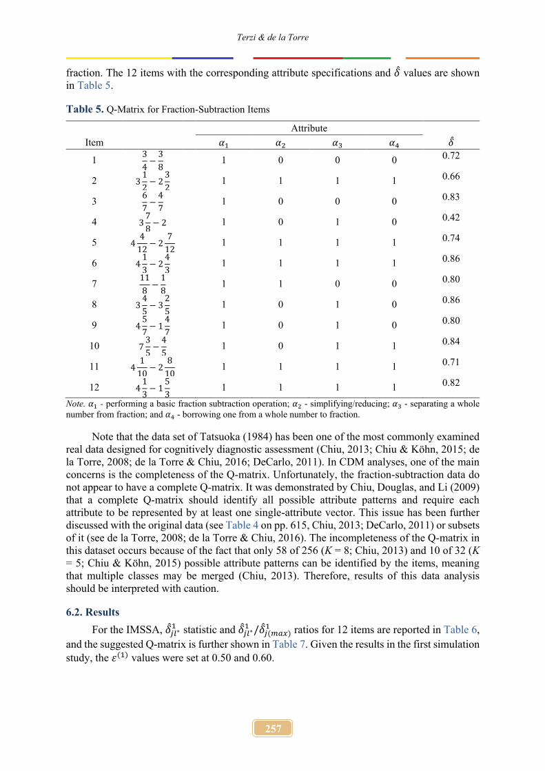
fraction. The 12 items with the corresponding attribute specifications and �̂� values are shown in Table 5.
Table 5. Q-Matrix for Fraction-Subtraction Items
Attribute Item 𝛼1 𝛼2 𝛼3 𝛼4 �̂�
1 3
4−
3
8 1 0 0 0 0.72
2 31
2− 2
3
2 1 1 1 1 0.66
3 6
7−
4
7 1 0 0 0 0.83
4 37
8− 2 1 0 1 0 0.42
5 44
12− 2
7
12 1 1 1 1 0.74
6 41
3− 2
4
3 1 1 1 1 0.86
7 11
8−
1
8 1 1 0 0 0.80
8 34
5− 3
2
5 1 0 1 0 0.86
9 45
7− 1
4
7 1 0 1 0 0.80
10 73
5−
4
5 1 0 1 1 0.84
11 41
10− 2
8
10 1 1 1 1 0.71
12 41
3− 1
5
3 1 1 1 1 0.82
Note. 𝛼1 - performing a basic fraction subtraction operation; 𝛼2 - simplifying/reducing; 𝛼3 - separating a whole number from fraction; and 𝛼4 - borrowing one from a whole number to fraction.
Note that the data set of Tatsuoka (1984) has been one of the most commonly examined real data designed for cognitively diagnostic assessment (Chiu, 2013; Chiu & Köhn, 2015; de la Torre, 2008; de la Torre & Chiu, 2016; DeCarlo, 2011). In CDM analyses, one of the main concerns is the completeness of the Q-matrix. Unfortunately, the fraction-subtraction data do not appear to have a complete Q-matrix. It was demonstrated by Chiu, Douglas, and Li (2009) that a complete Q-matrix should identify all possible attribute patterns and require each attribute to be represented by at least one single-attribute vector. This issue has been further discussed with the original data (see Table 4 on pp. 615, Chiu, 2013; DeCarlo, 2011) or subsets of it (see de la Torre, 2008; de la Torre & Chiu, 2016). The incompleteness of the Q-matrix in this dataset occurs because of the fact that only 58 of 256 (K = 8; Chiu, 2013) and 10 of 32 (K = 5; Chiu & Köhn, 2015) possible attribute patterns can be identified by the items, meaning that multiple classes may be merged (Chiu, 2013). Therefore, results of this data analysis should be interpreted with caution.
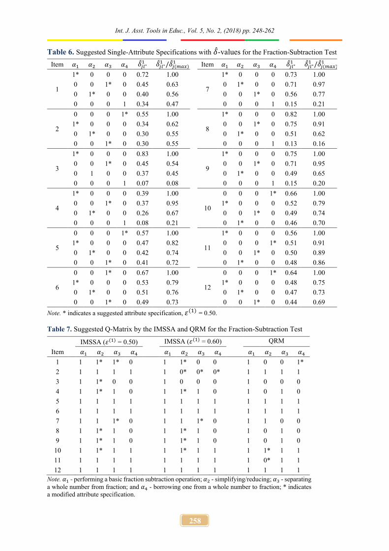
6.2. Results For the IMSSA, �̂�𝑗𝑙∗
1 statistic and �̂�𝑗𝑙∗1 /�̂�𝑗(𝑚𝑎𝑥)
1 ratios for 12 items are reported in Table 6, and the suggested Q-matrix is further shown in Table 7. Given the results in the first simulation study, the 휀(1) values were set at 0.50 and 0.60.
Int. J. Asst. Tools in Educ., Vol. 5, No. 2, (2018) pp. 248-262
258
Table 6. Suggested Single-Attribute Specifications with �̂�-values for the Fraction-Subtraction Test
Item 𝛼1 𝛼2 𝛼3 𝛼4 𝛿𝑗𝑙∗1 𝛿𝑗𝑙∗
1 /�̂�𝑗(𝑚𝑎𝑥)1 Item 𝛼1 𝛼2 𝛼3 𝛼4 𝛿𝑗𝑙∗
1 𝛿𝑗𝑙∗1 /�̂�𝑗(𝑚𝑎𝑥)
1
1
1* 0 0 0 0.72 1.00
7
1* 0 0 0 0.73 1.00 0 0 1* 0 0.45 0.63 0 1* 0 0 0.71 0.97 0 1* 0 0 0.40 0.56 0 0 1* 0 0.56 0.77 0 0 0 1 0.34 0.47 0 0 0 1 0.15 0.21
2
0 0 0 1* 0.55 1.00
8
1* 0 0 0 0.82 1.00 1* 0 0 0 0.34 0.62 0 0 1* 0 0.75 0.91 0 1* 0 0 0.30 0.55 0 1* 0 0 0.51 0.62 0 0 1* 0 0.30 0.55 0 0 0 1 0.13 0.16
3
1* 0 0 0 0.83 1.00
9
1* 0 0 0 0.75 1.00 0 0 1* 0 0.45 0.54 0 0 1* 0 0.71 0.95 0 1 0 0 0.37 0.45 0 1* 0 0 0.49 0.65 0 0 0 1 0.07 0.08 0 0 0 1 0.15 0.20
4
1* 0 0 0 0.39 1.00
10
0 0 0 1* 0.66 1.00 0 0 1* 0 0.37 0.95 1* 0 0 0 0.52 0.79 0 1* 0 0 0.26 0.67 0 0 1* 0 0.49 0.74 0 0 0 1 0.08 0.21 0 1* 0 0 0.46 0.70
5
0 0 0 1* 0.57 1.00
11
1* 0 0 0 0.56 1.00 1* 0 0 0 0.47 0.82 0 0 0 1* 0.51 0.91 0 1* 0 0 0.42 0.74 0 0 1* 0 0.50 0.89 0 0 1* 0 0.41 0.72 0 1* 0 0 0.48 0.86
6
0 0 1* 0 0.67 1.00
12
0 0 0 1* 0.64 1.00 1* 0 0 0 0.53 0.79 1* 0 0 0 0.48 0.75 0 1* 0 0 0.51 0.76 0 1* 0 0 0.47 0.73 0 0 1* 0 0.49 0.73 0 0 1* 0 0.44 0.69
Note. * indicates a suggested attribute specification, 휀(1) = 0.50.
Table 7. Suggested Q-Matrix by the IMSSA and QRM for the Fraction-Subtraction Test IMSSA (휀(1) = 0.50) IMSSA (휀(1) = 0.60) QRM
Item 𝛼1 𝛼2 𝛼3 𝛼4 𝛼1 𝛼2 𝛼3 𝛼4 𝛼1 𝛼2 𝛼3 𝛼4 1 1 1* 1* 0 1 1* 0 0 1 0 0 1* 2 1 1 1 1 1 0* 0* 0* 1 1 1 1 3 1 1* 0 0 1 0 0 0 1 0 0 0 4 1 1* 1 0 1 1* 1 0 1 0 1 0 5 1 1 1 1 1 1 1 1 1 1 1 1 6 1 1 1 1 1 1 1 1 1 1 1 1 7 1 1 1* 0 1 1 1* 0 1 1 0 0 8 1 1* 1 0 1 1* 1 0 1 0 1 0 9 1 1* 1 0 1 1* 1 0 1 0 1 0
10 1 1* 1 1 1 1* 1 1 1 1* 1 1 11 1 1 1 1 1 1 1 1 1 0* 1 1 12 1 1 1 1 1 1 1 1 1 1 1 1
Note. 𝛼1 - performing a basic fraction subtraction operation; 𝛼2 - simplifying/reducing; 𝛼3 - separating a whole number from fraction; and 𝛼4 - borrowing one from a whole number to fraction; * indicates a modified attribute specification.

Terzi & de la Torre
259
The results of the fraction-subtraction data obtained from the IMSSA were compared to the QRM. The IMSSA suggested attribute changes in seven items (i.e., items 1, 3, 4, 7, 8, 9, and 10) when 휀(1) = 0.50; whereas, the QRM suggested attribute changes in three items (i.e., items 1, 10, and 11). Based on the IMSSA, the result indicated that item 1 (i.e., 3
4−
3
8) should
require two more attributes (i.e., 𝛼2 and 𝛼3) in addition to 𝛼1. This suggestion may have occurred because this item requires more than just 𝛼1, performing a basic fraction subtraction problem. Another suggestion was for item 3 (i.e., 6
7−
4
7), where 𝛼2 was deemed required. Items
4 (i.e., 3 7
8− 2), 8 (i.e., 3 4
5− 3
2
5), 9 (i.e., 4 5
7− 1
4
7), and 10 (i.e., 7 3
5−
4
5) required 𝛼2 in addition
to 𝛼1and 𝛼3. Note that another strategy for solving the problem in one of these four items – borrowing one from a whole number to fraction, performing a basic fraction, and simplifying/reducing – happens to give the correct answer. The following example shows another strategy to solve item 9:
45
7− 1
4
7=
(4 × 7) + 5
7−
(1 × 7) + 4
7
=33 − 11
7=
22
7= 3
1
7 .
Another attribute suggestion (i.e., 𝛼3) was for item 7 (i.e., 11
8−
1
8) on the top of 𝛼1 and
𝛼2. Similar to the preceding example, a different strategy – separating a whole number from fraction, performing a basic fraction subtraction operation, and simplifying/reducing – could also give the correct answer to item 7, as in,
11
8−
1
8= 1
3
8−
1
8= 1
3 − 1
8
= 12
8= 1
1
4 .
In applying the QRM, Chiu (2013) found that item 4, which appears as item 2 in this
study, did not require the possession of 𝛼3 to be correctly answered. In contrast, the QRM in this study suggested that 𝛼3 was necessary. An explanation could be because of the fact that Chiu (2013) used 20 items with 8 attributes. Whereas, the IMSSA indicated that the mastery of the third attribute was required to answer item 2 correctly. The QRM also suggested to include and exclude 𝛼2 in items 10 and 11, respectively.
As demonstrated by the examples, a deeper analysis is needed. The IMSSA has more 1s than the QRM that can be controlled by adjusting the cut-offs. The cut-off values defined in the simulation study do not perfectly fit to the real data analysis in this case because it did not have a complete Q-matrix. The latter values were just approximations based on the conditions defined in the simulation study. Further discussions about multiple strategies in cognitive diagnosis using the fraction subtraction data can be found in de la Torre and Douglas (2008), Hou and de la Torre (2014), and Mislevy (1996). Other reasons could be because the fraction subtraction data have fewer number of items and attributes than the simulation study. Also note that when 휀(1) was set at 0.60, three items presented different attribute specifications (i.e., items 1, 2, and 3). 𝛼3 in item 1, and 𝛼2, 𝛼3, and 𝛼4 in item 2 were altered to 0s; however attribute specifications in item 3 was consistent with the Q-matrix given for the data.
Int. J. Asst. Tools in Educ., Vol. 5, No. 2, (2018) pp. 248-262
260
7. DISCUSSION AND CONCLUSION CDMs aim to classify the attribute mastery or nonmastery of examinees, and the Q-
matrix is needed for specifying required attributes for each item in a test. The importance of revising attribute specifications in the Q-matrix should not be underestimated due to the inherent subjectivity of domain experts, consequently resulting in serious validity concerns.
The IMSSA for Q-matrix validation presented in this study aimed to extend the SSA (de la Torre, 2008) in several ways. First, it offered a more efficient solution as it only examines the first K single-attribute q-vectors. Second, in addition to less number of computational requirements, an iterative algorithm was included in the method to decrease negative effects of any misspecified attribute specification given in the previous iteration. And, third, an approximation was made to generally define optimal cut-off values applicable across the specific set of conditions.
In this work, three methods without an iterative algorithm were compared to two methods with an iterative algorithm. Among the noniterative methods, the MSSA reported better results, which had higher recovery than the QRM on average across all the factors. As expected, the results showed that the IMSSA worked much better than the noniterative methods. According to the simulation studies, the IMSSA showed promising improvements in Q-matrix validation that could enhance the estimation of model parameters, model-data fit analyses, and ultimately, the accuracy of attribute-classifications.
Using a 3.50-GHz I7 computer, it took the code the least amount of time to run the validation procedures for MSSA, followed by IMSSA, ESA, SSA, and QRM. For instance, it took 1.64, 3.11, 9.89, 24.35, and 30.00 minutes using MSSA, IMSSA, ESA, SSA, and QRM procedures, respectively, for 100 iterations under the condition in that N = 2,000, J = 30, and medium quality items with 10% misspecifications in the Q-matrix.
This present study had some limitations. For instance, the number of attributes was assumed to be known and fixed to K = 5. It would be interesting to investigate the method by relaxing this assumption. The findings of this study were based on the attribute structure generated from a uniform distribution. The performance of the methods should be investigated under a condition where attributes were generated from a higher order distribution (de la Torre & Douglas, 2004). Also, in addition to the δ-statistic used in this study, other statistics can be carried out for Q-matrix validation. This study should also be extended to make it applicable to a wider class of CDMs such as the G-DINA model (de la Torre, 2011). This will obviate the need to assume the specific CDMs involved. Finally, this method should be applied to other real data sets (e.g., Akbay, Terzi, Kaplan, & Karaaslan, 2018) with a complete Q-matrix so that further insights can be gained on how the proposed method could work in practice.
ORCID Ragip Terzi https://orcid.org/0000-0003-3976-5054 Jimmy de la Torre https://orcid.org/0000-0002-0893-3863
8. REFERENCES Akbay, L., Terzi, R., Kaplan, M., & Karaaslan, K. G. (2018). Expert-based attribute
identification and validation: An application of cognitively diagnostic assessment. Journal on Mathematics Education, 9, 103-120.
Chiu, C. (2013). Statistical refinement of the Q-matrix in cognitive diagnosis. Applied Psychological Measurement 37, 598-618.
Chiu, C., & Douglas, J. (2013). A nonparametric approach to cognitive diagnosis by proximity to ideal response patterns. Journal of Classification 37, 225-250.

Terzi & de la Torre
261
Chiu, C., Douglas, J., & Li, X. (2009). Cluster analysis for cognitive diagnosis: Theory and applications. Psychometrika. 74, 633-665.
Chiu, C.-Y., & Köhn, H.-F. (2015). Consistency of cluster analysis for cognitive diagnosis: The DINO model and the DINA model revisited. Applied Psychological Measurement, 39, 465-479.
DeCarlo, L. T. (2011). On the analysis of fraction subtraction data: The DINA model, classification, latent class sizes, and the Q-matrix. Applied Psychological Measurement, 35(1), 8-26.
de la Torre, J. (2008). An empirically based method of Q-Matrix validation for the DINA model: development and applications. Journal of Educational Measurement, 45, 343-362.
de la Torre, J. (2009a). A cognitive diagnosis model for cognitively based multiple-choice options. Applied Psychological Measurement, 33, 163-183.
de la Torre, J. (2009b). DINA model and parameter estimation: A didactic. Journal of Educational and Behavioral Statistics, 34, 115-130.
de la Torre, J. (2011). The generalized DINA model framework. Psychometrika, 76, 179-199. de la Torre, J., & Chiu, C.-Y. (2016). A general method of empirical Q-matrix validation.
Psychometrika, 81, 253-273. de la Torre, J., & Douglas, J. A. (2004). Higher-order latent trait models for cognitive diagnosis.
Psychometrika, 69, 333-353. de la Torre, J., & Douglas, J. A. (2008). Model evaluation and multiple strategies in cognitive diagnosis: An analysis of fraction subtraction data. Psychometrika, 73, 595-624. Doornik, J. A. (2009). An object-oriented matrix programming language Ox 6. [Computer
software]. London, UK: Timberlake Consultants Ltd. Haertel, E. H. (1989). Using restricted latent class models to map the skill structure of
achievement items. Journal of Educational Measurement, 26, 333–352. Hou, L., de la Torre, J., & Nandakumar, R. (2014). Differential item functioning assessment in
cognitive diagnostic modeling: Application of the wald test to investigate DIF in the DINA model. Journal of Educational Measurement, 51, 98-125.
Huo, Y., & de la Torre, J. (2014). Estimating a cognitive diagnostic model for multiple strategies via the EM algorithm. Applied Psychological Measurement, 38, 464-485.
Junker, B. W., & Sijtsma, K. (2001). Cognitive assessment models with few assumptions, and connections with nonparametric item response theory. Applied Psychological Measurement, 25, 258-272.
Kuo, B.-C., Pai, H.-S., & de la Torre, J. (2016). Modified cognitive diagnostic index and modified attribute-level discrimination index for test construction. Applied Psychological Measurement, 40, 315-330.
Liu, J., Xu, G., & Ying, Z. (2012). Data-driven learning of Q-matrix. Applied Psychological Measurement, 36, 609-618.
Liu, J., Ying, Z., & Zhang, S. (2015). A rate function approach to computerized adaptive testing for cognitive diagnosis. Psychometrika, 80, 468-490.
Mislevy, R. J. (1996). Test theory reconceived. Journal of Educational Measurement, 33, 379-416.
Park, Y. S., & Lee, Y.-S. (2014). An extension of the DINA model using covariates examining factors affecting response probability and latent classification. Applied Psychological Measurement, 38, 376-390.
Int. J. Asst. Tools in Educ., Vol. 5, No. 2, (2018) pp. 248-262
262
R Core Team. (2014). R: A language and environment for statistical computing [Computer software manual]. Vienna, Austria. Retrieved from http://www.R-project.org/
Rojas, G., de la Torre, J., & Olea, J. (2012, April). Choosing between general and specific cognitive diagnosis models when the sample size is small. Paper presented at the annual meeting of the National Council of Measurement in Education, Vancouver, British Columbia, Canada.
Rupp, A., & Templin, J. (2008). Effects of Q-matrix misspecification on parameter estimates and misclassification rates in the DINA model. Educational and Psychological Measurement, 68, 78-98.
Tatsuoka, K. K. (1983). Rule-space: an approach for dealing with misconceptions based on item response theory. Journal of Educational Measurement, 20, 345-354.
Tatsuoka, K. K. (1984). Analysis of errors in fraction addition and subtraction problems (Report No. NIE-G-81-0002). Urbana: Computer-based Education Research Laboratory, University of Illinois.
Terzi, R. (2017). New Q-matrix validation procedures (Doctoral dissertation). Retrieved from https://doi.org/doi:10.7282/T3571G5G
Zheng, Y., & Chiu, C.-Y. (2015). NPCD: The R package for nonparametric methods for cognitive diagnosis.


